small-dollar children’s savings accounts and...

Campus Box 1196 One Brookings Drive St. Louis, MO 63130-9906 (314) 935.7433 csd.wustl.edu

Small-Dollar Children’s Savings

Accounts and College Outcomes

William Elliott University of Kansas

Subsequent publication: Elliott, W. (2013). Small-dollar children’s savings accounts and children’s college outcomes. Children and Youth Services Review,

35(3), 572–585.

2013

CSD Working Paper No. 13-05

SMALL-DOLLAR CHILDREN’S SAVINGS ACCOUNTS AND COLLEGE OUTCOMES

C E N T E R F O R S O C I A L D E V E L O P M E N T W A S H I N G T O N U N I V E R S I T Y I N S T . L O U I S

1

Acknowledgments Support for this paper comes from the Charles Stewart Mott Foundation. Other funders of research on college savings include the Ford Foundation, Citi Foundation, and Lumina Foundation for Education. The authors thank Margaret Clancy, Michael Sherraden, and Tiffany Trautwein at the Center for Social Development at Washington University in St. Louis for suggestions, reviews, and editing assistance.



2

Small-Dollar Children’s Savings Accounts and College Outcomes

In this paper, I examine the relationship between children’s small-dollar savings accounts and college enrollment and graduation by asking three important research questions: (a) are children with savings of their own more likely to attend or graduate from college, (b) does dosage (i.e., having no account; having basic savings only; having savings designated for school of less than $1, $1 to $499, or $500 or more) matter, and (c) is having savings designated for school more predictive than having basic savings alone? I use aggregate data from the newest wave of the Panel Study of Income Dynamics (PSID) and its supplements. Propensity score-weighted findings suggest that children who have a small amount of money (e.g., less than $1 or $1 to $499) designated for school are three times and two and a half times more likely, respectively, to enroll in and graduate from college than children with no account. Findings also show that having savings designated for school might have a stronger impact on children’s college outcomes than having basic savings. The paper concludes by explaining how federal policies might promote children’s savings and subsequent self-identification as college savers. Key words: saving, asset-building, wealth accumulation, low-income, child development accounts, children’s savings accounts, educational outcomes, college savings, college enrollment, college graduation, small-dollar accounts Highlights

A child with school savings of less than $1 is approximately three times more likely to enroll in college than a child with no savings.

A child with school savings of less than $1 is more than four and half times more likely to enroll in college than a child with only basic savings.

A child with school savings of $1 to $499 before reaching college age is almost two and half times more likely to graduate from college than a child with no savings.

Wealth-building policies to improve college enrollment and graduation rates might have positive effects even when children save only small amounts.

When examining whether a school savings program is effective, enrollment and graduation outcomes might be equal or better indicators of saving behaviors or amounts saved.

If one of the main goals is to improve children’s college enrollment and graduation outcomes, programs that create separate school accounts or encourage children to designate a portion of savings for school might be more effective than programs that promote saving without encouraging children to link savings mentally to college.



3

Introduction In 1991, Michael Sherraden proposed Child Development Accounts (CDAs) as a way to create an inclusive and accessible opportunity for lifelong savings and asset building. Specifically, CDAs have the potential to serve as a policy vehicle to allocate both intellectual and material resources to low- and moderate-income (LMI) children. Allocation of resources to LMI children is important because of disparity in the abilities of LMI parents and high-income (HI) parents to invest in their children. For example, Kornrich and Furstenberg (2010) find that Americans at the upper end of the income spectrum spend nine times as much per child as low-income families do. In their study, spending includes childcare, education, clothes, toys, and other child-related costs, investments that appear to matter for children’s educational outcomes. Entwisle, Alexander, and Olson (2005) find that differences in economic resources drive much of the racial-ethnic attainment gap. Controlling for other factors, minority and White students are equally likely to be enrolled in two- or four-year colleges at age 22. Baily and Dynarski (2011) examine two generations of students: those born from 1961 to 1964 and those born from 1979 to 1982. By 1989, one third of the HI students in the first generation had finished college. By 2007, more than half of the second generation had done so. However, only 9% of the low-income students in the second generation had completed college by 2007. Finding ways to allocate additional assets to LMI children might be particularly important. Elliott (2013) finds that children living in liquid and net worth asset-poor families have lower academic achievement scores, high school graduation rates, college enrollment rates, and college graduation rates than children living in families that are asset sufficient. He concludes, ―a bifurcated welfare system, with income-based programs for poor families and asset-based programs for higher income families, provides higher income families with an educational advantage over low-income families and might ultimately help exacerbate educational inequalities in America‖ (p. 15). Moreover, Elliott and Friedline (2012) find that 41% of students from low-income ($0 to $20,000) families report paying for college with family contributions while 81% of students from HI ($100,001 or higher) families report paying for college with family contributions. Given the disparities in investment in children by income level and the impact of having assets on college completion rates, finding ways to allocate resources—especially assets—to LMI children for human capital development appears worthwhile. Since 1991, when CDAs were first proposed, Singapore, the United Kingdom, South Korea, and Canada have initiated CDA policy efforts (Loke & Sherraden, 2009). In the United States, CDAs have been discussed as a promising asset-based approach for helping children think about their futures and prepare for college, but they have yet to be adopted at the national level. However, a number of legislative proposals have been developed, including the America Saving for Personal Investment, Retirement, and Education (ASPIRE) Act, Young Savers Accounts, 401Kids Accounts, Baby Bonds, and Portable Lifelong Universal Savings Accounts (Cramer, 2010). The ASPIRE Act is an example of what a large, universal children’s savings account effort would look like. ASPIRE would create Lifelong Savings Accounts for every newborn with an initial $500 deposit and opportunities for financial education. Children living in households with incomes below the national median would be eligible for an additional contribution of up to $500 at birth and a savings incentive of $500 per year in matched funds. When accountholders turn 18, they would be



4

permitted to make tax-free withdrawals for costs associated with post-secondary education, a first-time home purchase, and retirement security.1 National interest in the potential for CDAs to provide greater access to and completion of college for more children is evident in the rapidly changing U.S. Department of Education (DOE) policy on children’s savings. In November 2010, the DOE, Federal Deposit Insurance Corporation (FDIC), and National Credit Union Administration (NCUA) established a new federal partnership to encourage schools, financial institutions, federal grantees, and other stakeholders to work together to increase financial literacy, access to federally-insured bank accounts, and savings among students and families across the country.2 In 2011, as part of Gaining Early Awareness and Readiness for Undergraduate Programs (GEAR UP), the DOE announced an invitational priority that reflected Secretary of Education Arnie Duncan’s interest in financial literacy and savings as part of a plan for ensuring secondary school completion and postsecondary education enrollment of GEAR UP students. Of the 66 grants awarded, 42 included some aspect of financial literacy and savings in their applications. On May 31, 2012, the DOE announced a new college savings account research demonstration project, which will be implemented within the GEAR UP program. The demonstration will test the effectiveness of pairing new federally supported college savings accounts with GEAR UP activities against the effectiveness of standard GEAR UP activities that do not include college savings accounts. To support the demonstration, $8.7 million has already been allocated. Despite the growing interest in children’s savings, important questions remain unanswered. This study examines whether having only small amounts of money in savings accounts—small-dollar accounts—can have a positive effect on children’s college outcomes; whether having savings specifically for school is a stronger predictor of educational outcomes than having only basic savings; and if children’s savings (basic or school-designated) are associated with college graduation.3

Review of Research on Children’s Savings and College Outcomes Six studies discussed below (Advisory Committee on Student Financial Assistance [ACSFA], 2006; Elliott & Beverly, 2011a; Elliott, Choi, Destin, & Kim, 2011; Elliott, Chowa, & Loke, 2011; Elliott, Constance-Huggins, & Song, 2012; Elliott & Nam, 2012) are part of a growing body of work that may be particularly informative for developing CDA policies designed to help children accumulate assets and develop their own human capital.4 Before discussing specific findings on children’s

1 A description of the ASPIRE Act and its provisions can be found in Cramer and Newville (2009). 2 For more information, go to http://www.ed.gov/news/press-releases/fdic-and-ncua-chairs-join-education-secretary-announce-partnership-promote-finan. 3 I would like to thank Dr. Terri Friedline for suggesting the phrase ―small-dollar accounts.‖ 4 The idea of universal and progressive accounts made available at birth is being tested in a large randomized experiment called SEED for Oklahoma Kids (SEED OK). SEED OK aims to test whether (a) institutions for saving and asset accumulation can be extended successfully to the full population in a progressive rather than regressive manner and potentially over a lifetime and (b) this eventually increases savings, asset accumulation, attitudes and behaviors of parents, and attitudes, behaviors, and achievements of children (Nam, Kim, Clancy, Zager, & Sherraden, 2011). Such programs will provide a more direct test of CDA policies. However, because the accounts were opened in 2008 for newborns, researchers will not be able to test this design as it relates to college outcomes for several years.



5

savings and their relationship to college outcomes, it is important to provide some background information on the data used in these studies and how college outcomes and children’s savings have been measured. Panel Study of Income Dynamics The six studies reviewed in this paper use data from the Panel Study of Income Dynamics (PSID) and its supplements, the Child Development Supplement (CDS) and the Transition into Adulthood (TA) Study. This paper also uses data from the PSID and its supplements. The PSID, a nationally representative longitudinal survey of individuals and families, began in 1968 and collects data on employment, income, and assets. The CDS was administered to 3,563 PSID respondents in 1997 to collect a wide range of data on parents and their children aged birth to 12 years. It focuses on a broad range of developmental outcomes across the domains of health, psychological well-being, social relationships, cognitive development, achievement motivation, and education. Follow-up surveys were administered in 2002, 2007, and 2009. Children are followed by the CDS until they reach age 18 but do not join the core PSID until they become economically independent around age 25. The TA was designed to fill the gap between ages 18 and 25, an important time of life when youth decide whether to go to work or college.5 The TA measures outcomes for children who participated in earlier waves of the CDS and were no longer in high school. It was administered in 2005, 2007, and 2009. While the PSID and it supplements provide one of the few opportunities researchers have to examine the potential effects of children’s savings on educational outcomes, previous research on the subject has been limited to college enrollment and college progress/persistence. Until the 2009 wave of data was released, too few children in the TA had graduated from college to conduct a meaningful analysis of the relationship between savings and college graduation. College enrollment is measured as having ever enrolled in college at any point, and college progress is measured as either having graduated from college or currently being enrolled. College enrollment and college progress are important indicators to study because they reflect steps toward college graduation. For example, Baily and Dynarski (2011) find that inequality in college persistence explains a substantial share of inequality in college completion. Children must be prepared to enter college and able to persist in college if they are to graduate. People fail to persist at every stage, so interventions that have positive effects at any point are useful, and those that have positive effects at multiple stages might be especially effective for improving children’s outcomes and appealing to policymakers. In almost all college enrollment studies using the PSID, children’s savings has been measured either as a binary variable or a three-level variable. The CDS asks children between the ages of 12 and 18 whether they have a savings or bank account in their name. The children’s basic savings variable divides children into two categories: (a) those who had an account in 2002 and (b) those who did not. An account here refers to a basic savings account that can be opened at a local bank or credit union. Children who answer yes are asked whether they are saving some of this money for future education. The focus of college enrollment studies primarily has been whether children have savings

5 The age ranges are not exact. Some children leave high school earlier than others, and some children achieve economic independence later than others.



6

for future schooling (children’s school savings) (see Elliott & Beverly, 2011a; Elliott, Choi, Destin, & Kim, 2011; Elliott, Chowa, & Loke, 2011; Elliott, Constance-Huggins, & Song, 2012; Elliott & Nam, 2012). Children’s school savings has been operationalized in PSID studies as a binary variable with (a) children who have no account and children with only basic savings as the reference group and (b) children who have designated a portion of their basic savings for future school. This question in the CDS does not refer to having an actual savings account for school (e.g., a state 529 account) but rather to children’s mental accounting of savings, a topic that will be discussed more in the theoretical framework section of this paper. There are two exceptions to how children’s savings has been operationalized. In the first exception, researchers treat children’s savings as a three-level variable instead of a binary variable (has savings/does not have savings). For example, Elliott and Beverly (2011b) use a three-level variable with children who have (a) no account, (b) basic savings only, or (c) school savings. Using a three-level categorical variable allowed Elliott and Beverly to examine whether children’s basic savings and children’s school savings have individual effects on college enrollment (i.e., having ever enrolled), but it does not allow for a direct test of whether basic savings or school savings has more predictive power. In a study examining children’s math scores, Elliott, Jung, and Friedline (2011) suggest that having savings specifically for school purposes is likely to have a stronger effect on educational outcomes than basic savings. The evidence is mixed, however. While they find that children with basic savings have slightly higher math scores, the strength of the relationship varies by family net worth (e.g., children who live in higher net worth families score higher). In the case of school savings, the effects are the same regardless of net worth. Conversely, Elliott and Beverly (2011b) find evidence that both types of savings have a positive effect on children’s college enrollment, but basic savings has a stronger effect. One reason could be that Elliott and Beverly restrict their sample to children who expect—before reaching college age—to graduate from a four-year college. They suggest this could be because when children already expect to graduate from college, having savings specifically for college matters less. The second exception to how children’s savings is measured has to do with whether basic savings has different effects when children do and do not have positive college expectations. Elliott, Choi, Destin, & Kim (2011) use the binary basic savings-only variable, but they combine it with children’s college expectations to create dosages. More specifically, they create four doses: (a) children who have no savings and are uncertain whether they will graduate from a four-year college, (b) children who have basic savings only, (c) children who are certain only, and (d) children who have savings and are certain they will graduate from a four-year college. The reference group for each dosage is all other dosages. For example, the reference group for children who have basic savings only is children with no savings and are uncertain, children who are certain only, and children who have savings and are certain. The authors find when children do not expect to graduate college, basic savings is a negative predictor of college enrollment. But when children have basic savings and expect to graduate from college, having basic savings is a positive predictor of college enrollment. This supports the proposition that the type of savings they have matters less when children have positive college expectations. Several important differences exist between accounts examined in studies using the PSID and CDAs. CDAs proposed in the ASPIRE Act and other popular education accounts (e.g., Coverdell Education Savings Accounts, Uniform Gifts to Minors Act [UGMAs], 529 college savings plans run by states, and Roth Individual Retirement Arrangements [IRAs]) offer their owners protection from



7

taxation, and some have infrastructures that allow for direct deposit and provide savings matches to encourage saving. Savings in these accounts typically cannot be withdrawn without taxes or penalties until youth reach college age, and withdrawals must be spent on college-related expenses. As a result, these accounts can be defined as non-liquid. Unlike users of these popular education accounts, children in this study can withdraw and use money from their accounts without penalty, but they do not benefit from tax breaks or other incentives that are common components of CDAs (e.g., initial deposits or savings matches provided by the federal government or another agency). Moreover, the operationalization of children’s savings accounts in previous PSID studies has not answered questions from the media, policymakers, and the general public. After the announcement of the GEAR UP demonstration by the U.S. Department of Education, a reporter asked if $1,600 dollars would be enough to make a meaningful difference in a child’s life. Determining whether owning an account—even if money is not deposited into it—can change children’s educational outcomes would have strong implications and is an important question to address. This study will begin to examine that question. College enrollment findings Elliott and Beverly (2011a) examine whether children aged 17–23 who have already left high school are enrolled in or have graduated from a two-year or four-year college. Being currently enrolled in or having graduated from college is defined as being on course. Not currently being enrolled in or having graduated from college is defined as being off course. On average, 57% of children in the study are on course. However, 75% of children with their own savings are on course contrasted with 45% of children without savings. When factors such as race, family income, parent’s education, and children’s academic achievement are controlled for, children’s savings remains an important predictor of whether or not they are on course. In fact, findings indicate that 17–23-year-old children who have savings are approximately twice as likely to be on course as their peers without savings, which implies the importance of policies promoting large-scale children’s savings programs. Evidence from this study also indicates that children’s savings is connected with having a more positive college-bound identity, which shapes decisions about whether or not to remain on course. Policies that promote children’s savings may reduce fears that financial barriers will prevent them from staying on course. Elliott, Constance-Huggins, and Song (2012) ask whether the effects of savings for children’s on college progress differ between LMI (below $50,000) children and HI ($50,000 or above) children. Findings indicate that only 35% of LMI children are on course compared to 72% of HI children. Regarding children’s savings, 46% of LMI children with their own accounts are on course, while only 24% of LMI children without their own accounts are. When factors such as parents’ expectations and school involvement, family income, and children’s academic achievement are controlled for, the presence of children’s savings remains an important predictor of whether or not LMI children are on course. However, having savings is not an important predictor for HI children, which suggests that HI children are confident in their parents’ ability to pay for college. LMI children, however, may see their families being unable to pay bills, buy a washer and dryer, or afford groceries. An important implication is that using public funds to target



8

LMI children may be more impactful because these children may be more influenced to stay on course by the presence of a savings account than HI children would be. Elliott and Nam (2012) examine whether there are differences in effects of children’s savings by race.6 In particular, they examine whether or not Black and White children are on course. Among Black students, only 37% are on course compared to 62% of White students. When similar factors as those in the previous two studies are controlled for, Black and White children who have savings are about twice as likely to be on course as their counterparts without savings. This finding may be particularly important for Black children, who experience higher amounts of debt upon graduating from college on average. Twenty-seven percent of Black young adults who graduated from a four-year college in 2007–08 finished with $30,500 or more of debt in comparison to 15% of their White counterparts (Baum & Steele, 2010). Evidence shows that large levels of debt increase college dropout rates among Black students (Somers & Cofer, 2000). Therefore, having savings likely would lessen the debt load carried by a disproportionate number of Black students. The ACSFA (2006) examines the effect that financial constraints have on actual college attendance by identifying children who expect to attend college but do not do so soon after graduating from high school. Elliott and Beverly (2011b) call this phenomenon ―wilt.‖ In this study, wilt is used to describe the experience of children who have not attended a four-year college by 2005 despite holding expectations in high school in 2002 that they would attend and graduate. Findings from this study indicate that 55% of children without accounts of their own experience wilt, while only 20% of children with accounts do. After controlling for a variety of factors—including academic achievement—findings show that children who expect to graduate from a four-year college and have an account are about six times more likely to attend college than those who expect to graduate from a four-year college but do not have an account. Moreover, when children’s savings are added to the model, academic achievement is no longer statistically significant, which implies that desire and ability alone may not be enough for children to attend college. In an earlier report to Congress, ACSFA (2001) draws a similar conclusion stating, ―Make no mistake, the pattern of educational decision making typical of low-income students today, which diminishes the likelihood of ever completing a bachelor’s degree, is not the result of free choice. Nor can it be blamed on academic preparation‖(p. 18). Elliott, Choi, Destin, and Kim (2011) examine whether having savings leads to more positive expectations or whether more positive expectations lead to children having savings. This is an important question related to the potential of CDAs to have indirect effects. While this study could not establish a causal link between children’s savings and their expectations for college, it does provide evidence that having savings might lead to more positive college expectations among children. However, the most accurate interpretation might be that two-way causation exists (i.e., children’s savings leads to more positive college expectations, and more positive college expectations leads to children having savings of their own).

6 However, an important limitation of the PSID and CDS is that low-income families are disproportionately represented among Black households, and very few high-income Black households are included in the sample. As a result, findings using samples of Blacks only are probably more indicative of low-income Blacks than all Blacks.



9

Elliott, Chowa, and Loke (2011) build on Elliott, Choi, Destin, and Kim (2011) and ask whether a combined approach that promotes children’s savings and positive college expectations is more effective than either strategy alone. To test this, the study divides children into four groups: (a) those with no school savings who are uncertain before leaving high school whether they would graduate from a four-year college, (b) those who have school savings and are uncertain before leaving high school whether they would graduate from a four-year college, (c) those who have no school savings and are certain before leaving high school they would graduate from a four-year college, and (d) those who have school savings and are certain before leaving high school they would graduate from a four-year college. Findings support the hypothesis that having savings is more effective when children expect to graduate from college. Summary Overall, findings from these studies suggest that programs promoting children’s savings have a positive effect on children’s college enrollment. Evidence to date suggests that positive effects are more likely to occur for LMI children than HI children. There appears to be a point at which household income is high enough that having savings makes no statistical difference in whether children have graduated from college or are currently progressing toward graduation. This may be because beyond a certain income threshold, children do not doubt that their families will be able to pay for college. Findings also suggest that having a stake in college (i.e., owning savings) has a positive effect on Black children’s college progress.

Small-Dollar Accounts Can Create Psychological Effects In this section, I use theories of mental accounting and identity-based motivation (IBM) to lay out a theoretical framework for understanding how small-dollar accounts can lead to positive educational outcomes. I also begin to describe why we might expect basic savings to have different effects on children’s educational outcomes than school savings. I conclude by stating the primary research questions that flow from this framework and are examined in this study. Mental accounting Mental accounting has been described as the process of dividing current and future money into different categories to monitor spending (Thaler, 1985). Behavioral economists suggest that people use mental accounting techniques to think about different pots of money, which affects when and how they use it (Kahneman & Tversky, 1979; Lea, Tarpy, & Webley, 1987; Thaler, 1985; Winnett & Lewis, 1995; Xiao & Anderson, 1997). In other words, different mental or physical accounts have different purposes and meanings that affect how people deposit money into the accounts and use it (Winnett & Lewis,1995). However, I suggest that the process of creating mental accounts might affect formation of actionable identities, which in turn might help explain how small-dollar accounts can positively affect children’s educational outcomes.7

7 Oyserman and Destin (2010) suggest children do not always act on an identity.



10

Explaining the effects of small-dollar accounts and the role of IBM IBM is a theory about how identities are formed and which identities people will act on. IBM theorists suggest that three principal components affect the relationship between self-conceptions and motivation and give significant attention to how social and cultural context drives the process. The three core principles of IBM include (a) identity salience, (b) congruence with group identity, and (c) interpretation of difficulty (Oyserman & Destin, 2010). Salience is the idea that children are more likely to work toward a goal when images of their own future are at the forefront of their mind. Congruence with group identity occurs when an image of the self feels tied to ideas about relevant social groups (e.g., friends, classmates, family, and cultural groups). When this occurs, the congruent personal identity is reinforced. IBM theorists highlight the importance of having a means for normalizing and overcoming difficulty. From this perspective, in order for children to sustain effort and work toward a self-image (e.g., college-bound), they and their environment must provide ways to address inevitable obstacles (e.g., financing college). These principles have been found to be important predictors of children’s school behaviors (Oyserman & Destin, 2010). The IBM framework can be used to understand how designating small amounts of money for school (mental accounting) can lead to positive educational outcomes. How might this happen? I suggest that the mental accounting categorization process (i.e., designating savings for school) helps children manifest abstract conceptions of the self (e.g., college-bound). According to the principles of IBM—identity salience, congruence with group identity, and interpretation of difficulty—mentally designating savings for college, regardless of the amount, indicates that college is the child’s goal and expectation and the child sees saving as a relevant behavioral strategy for overcoming the difficulty of paying for college. Even small-dollar accounts may signal to a child that financing college is possible despite the high cost because the child may be considering future expected savings not current savings. From this perspective, expected savings might be as important as current savings—or at least a sufficient reason—for believing that college is within reach and requires current action.8 Finally, designating money for college indicates that children recognize that people like them can go to college and that they are ready to take action to fulfill the college-bound identity. Basic savings versus school savings As stated in the research review section, children’s savings measured in studies using the PSID and its supplements are not in school-specific accounts but rather in basic savings accounts that children have designated mentally for school purposes. The process of mentally designating savings for school leads to the formation of what I refer to as a college-saver identity. Being a college saver indicates—more accurately than being college bound—that the child has identified saving as a strategy to attain the future goal of college attendance. Distinguishing between having a college-bound identity and a college-saver identity acknowledges that children can perceive of themselves as being college-bound without having a strategy for overcoming the difficulty of paying for college (i.e., they might not have linked saving to college or may not be able to trust that their families will pay for college).

8 For more information about the concept of future expected savings, see Sherraden (1991).



11

When children mentally designate savings for college, they are more likely to have made the link between saving and paying for college. While I cannot directly test this proposition in this study, evidence suggests that children’s savings programs might help children link saving to paying for college. Elliott, Sherraden, Johnson, and Guo (2010) find that the proportion of second graders in a comparison group who mentioned savings as important (20%) was approximately the same as that of second graders in a treatment group (23%) in a children’s savings program called ―I Can Save.‖ By fourth grade, I Can Save children far more commonly mentioned savings as being important to their ability to finance college (74%) than comparison group children (25%). The embedded process or strategy in this case is most simply stated by a lower income student who said, ―Well, I’m going to pay for [college], because I have my own bank account‖ (Elliott et al., 2010, p. 6). When children designate savings for school, they are more likely to see themselves as being college-bound, but I posit that the college-saver identity is a better predictor of not only college attendance but also completion. A body of literature suggests that low-income and minority children who expect to attend college often fail to enroll (Elliott & Beverly, 2011b; Schneider & Stevenson, 1999; Trusty, 2000). According to Elliott and Beverly (2011b), children who have college-saver identities are much more likely to act on them than those with only college-bound identities without a strategy. This suggests that not all identities are equally actionable. A potentially important difference exists between being in a children’s savings program and simply designating savings for school. Unlike a savings program in which children might be signed up by their parents or see it as an opportunity to spend time with friends, designating money for college involves thinking actively about college and saving (i.e., identity salience), understanding that others like the child go to college (i.e., group congruence), and viewing college as an important goal and saving as a way to pay for it (i.e., interpretation of difficulty as normal). In this way, designation of money for college appears to align with the three main principles of IBM.9 For the purpose of this study, I assume that children who have designated savings for school have made the link between saving and paying for college. In contrast, I do not assume that a child with a basic savings account who does not report designating some money for college sees saving as a way to pay for college or that college is important.10 Basic savings accounts can be opened and used for many different purposes. Therefore, I posit savings designated for school should be more closely associated with educational outcomes than basic savings. Situation sensitivity – the financial context and why children save IBM theorists suggest that while children act in ways that fit their possible selves, identities are highly situation sensitive. It might be that before and after the process of categorization (i.e., formation of an identity as a college saver) takes place, the level of financial need helps provide the situational context for actual allocation of earnings to mental accounts (see Xiao & Anderson,

9 For information about IBM and school engagement, see Oyserman and Destin (2010). 10 This might suggest that CDA programs need to develop financial education curriculums, for example, or build in other ways that help children adopt mental accounting techniques.



12

1997).11 This helps explain why children might not save (or designate savings from) current income in their school savings account or might save very little. As described by Xiao and Anderson (1997), Maslow contends that people will attempt to fulfill higher level needs (e.g., by saving for college education) only after lower level needs (e.g., purchasing groceries and paying bills) have been met. From this perspective, needs are categorized into two types: deficit (e.g., lower level) needs and growth (e.g., higher level) needs. People seek to fulfill their deficit needs first and then begin to direct their behavior toward fulfilling growth needs. Building on Maslow’s theory, Xiao and Anderson (1997) identify three categories of financial need based on tolerance for risk taking: survival needs, security needs, and growth needs. The categories are based on research conducted by Xiao and Noring (1994), who find that low-income consumers are more likely to report saving for daily expenses (survival needs), middle-income consumers are more likely to report saving for emergencies (security needs), and high-income consumers are more likely to report saving for growth. Assuming various financial accounts can be used to represent different financial needs, I posit that savings vehicles designated exclusively to growth needs (e.g., education) may have less of an impact than basic savings accounts on the saving behavior of children in disadvantaged households. This is not to suggest that disadvantaged children do not perceive the value of fulfilling growth needs but rather that their actual saving behaviors are likely to reflect a need to fulfill survival needs. This raises questions about whether amount saved is the right variable to study when evaluating the effectiveness of children’s savings accounts for improving college outcomes. Evidence suggests that having an account might be as important as the amount in the account for children’s college outcomes. Jackson (1978) finds that simply receiving a financial aid award can be more influential in whether a child enrolls in college than the amount of the award. In this study, I examine the potential of small-dollar accounts—not the amounts in them—to have positive effects on children’s college outcomes.

Research Questions The following three research questions flow out of the theoretical framework outlined above: (a) are children with savings of their own more likely to attend or graduate from college, (b) does dosage (i.e., having no account; having basic savings only; or having designated savings for school of less than $1, $1 to $499, or $500 or more) matter, and (c) is designating savings for school more predictive than having basic savings alone?

Methods Data This study uses data from the PSID and its supplements, the CDS and TA, which are discussed in more detail earlier in this paper. The three data sets are linked using PSID, CDS, and TA map files containing family and personal ID numbers. The linked data sets provide a rich opportunity for

11 Before and after identity formation takes place, financial need may affect the process and help determine what mental categories are formed. After they are formed, it also might affect decisions about into which account current savings should be allocated.



13

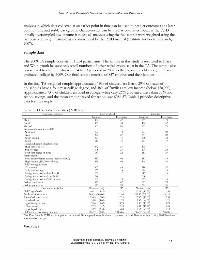
analyses in which data collected at an earlier point in time can be used to predict outcomes at a later point in time and stable background characteristics can be used as covariates. Because the PSID initially oversampled low-income families, all analyses using the full sample were weighted using the last observed weight variable as recommended by the PSID manual (Institute for Social Research, 2007). Sample data The 2009 TA sample consists of 1,554 participants. The sample in this study is restricted to Black and White youth because only small numbers of other racial groups exist in the TA. The sample also is restricted to children who were 14 to 19 years old in 2002 so they would be old enough to have graduated college by 2009. Our final sample consists of 857 children and their families. In the final TA weighted sample, approximately 19% of children are Black, 29% of heads of households have a four-year college degree, and 48% of families are low income (below $50,000). Approximately 73% of children enrolled in college, while only 26% graduated. Less than 50% had school savings, and the mean amount saved for school was $386.57. Table 1 provides descriptive data for the sample. Table 1. Descriptive statistics (N = 857)

Categorical variables Non-weighted Weighted

Number Percentage Number Percentage

Black 404 47 163 19 Female 460 54 442 52 Married 553 65 641 75 Region of the country in 2003 Northeast 122 14 173 20 West 228 27 244 29 North central 397 46 276 32 South 110 13 161 19 Household head’s education level High school or less 472 55 400 47 Some college 198 23 204 24 Four-year degree or more 187 22 251 29 Family income Low- and moderate-income (below $50,000) 512 60 411 48 High-income ($50,000 or above) 345 40 444 52 Child’s savings dosages No account 407 48 318 37 Only basic savings 152 18 196 23 Savings for school w/less than $1 100 12 115 13 Savings for school w/$1 to $499 90 11 93 11 Savings for school w/$500 or more 108 13 133 16 College enrollment 575 67 623 73 College graduation 175 20 224 26

Continuous variables Mean (median) SD Mean (median) SD

Child’s age (2002) 16.11 (16.10) 1.52 16.11 (16.02) 1.50 Academic achievement 203.31 (200.00) 31.44 211.43 (209.00) 31.19 Parents’ education level 13.03 (12.00) 2.25 13.43 (13.00) 2.36 Household size 3.88 (4.00) 1.29 3.85 (4.00) 1.21 Log of family income 9.26 (10.62) 3.73 9.85 (10.87) 3.28 IHS net worth 7.92 (11.12) 7.33 9.31 (11.70) 6.48 Log of liquid assets 5.09 (7.49) 5.84 6.53 (8.37) 5.19 Children’s school savings amount 386.57 (0.00) 1,106.86 386.57 (0.00) 1,106.86

Note: Data from the PSID and its supplements are used. Data imputed using the chained regression method. Data are weighted using 2009 Transition into Adulthood weight. Variables



14

The variable of interest in this study is children’s savings, created using 2002 CDS data. The CDS asks children between the ages of 12 and 18 whether they have a physical savings or bank account in their name. The children’s basic savings variable divides children into two categories: (1) those who had an account in 2002 and (2) those who did not have an account. Children with accounts were asked whether they were saving some of this money for future schooling (i.e., whether they had mentally set aside some savings for school). Children who replied yes were asked the amount of savings they had for future schooling between $.01 and $9,997.99. Using the two children’s savings variables and the amount saved for school variable, I created five treatment groups, or doses, similar to Imbens’ (2000) multiple-dose treatment approach (see also Guo & Fraser, 2010). The doses are children with (a) no savings, (b) basic savings only, (c) school savings of less than $1, (d) school savings of $1 to $499, and (e) school savings of $500 or more. Outcome variables The two outcome variables in this study are college enrollment and college graduation. College enrollment is operationalized as whether or not a child had ever enrolled in college by 2009 (1 = yes; 2 = no). College graduation measures whether a child had graduated from college by 2009 (yes = 1; no = 0). In this study, college refers to either a two- or four-year college. Control variables There are 11 control variables used in this study, including child’s age in 2002, child’s race (1 = Black; 0 = White), child’s gender (female = 1; male = 0), child’s academic achievement, head of household’s marital status in 2003 (1 = married; 0 = not married), head of household’s education level in 2003, household size in 2003 (continuous variable), region of the country in which the family lived in 2003, log of household income, inverse hyperbolic sine of household net worth, and log of liquid assets. Log of household income. The log of household income was created using income variables from 1989, 1994, 1999, 2004, and 2009 and inflated to 2009 price levels using the Consumer Price Index (CPI). Income variables were averaged across all five years, and average income was transformed using the natural log transformation to account for the skewedness of the variable. Inverse hyperbolic sine of household net worth. Household net worth is a continuous variable that sums all assets, including savings, stocks/bonds, business investments, real estate, home equity, and other assets and subtracts all debts, including credit cards, loans, and other debts as reported in the 1989, 1994, 1999, and 2001 PSIDs. I use the inverse hyperbolic sine (IHS) transformation (Kennickell & Woodburn, 1999), which allows for the existence of negative values and more clearly demonstrates changes in wealth distribution (Kennickell & Woodburn, 1999). The natural log transformation does not. Head of household’s education level. In the PSID, the head of household’s education level is a continuous variable (1–16) with each number representing a year of completed schooling. Region. This variable captures the region in which a child’s family lived at the time of the 2003 interview, including the Northeast, North Central, South, and West regions of the country.



15

Northeast includes Connecticut, Maine, Massachusetts, New Hampshire, New Jersey, New York, Pennsylvania, Rhode Island, and Vermont. North Central includes Illinois, Indiana, Iowa, Kansas, Michigan, Minnesota, Missouri, Nebraska, North Dakota, Ohio, South Dakota, and Wisconsin. South includes Alabama, Arkansas, Delaware, the District of Columbia, Florida, Georgia, Kentucky, Louisiana, Maryland, Mississippi, North Carolina, Oklahoma, South Carolina, Tennessee, Texas, Virginia, and West Virginia. West includes Arizona, California, Colorado, Idaho, Montana, Nevada, New Mexico, Oregon, Utah, Washington, and Wyoming. The Northeast region is the reference group for this study. Academic achievement. This is a continuous variable that combines math and reading scores. The Woodcock Johnson (WJ-R), a well-respected measure, is used by the CDS to assess math and reading ability (Mainieri, 2006). In descriptive analysis, I use a dichotomous variable indicating whether children had average, above-average, or below-average achievement. Average and above-average achievement are coded as 1, and below-average achievement is coded as 0. Child’s age. Age in 2002 is a continuous variable. In the descriptive analysis, a dichotomous variable indicates whether children were 16 years old or younger (coded as 0) or older than 16 years (coded as 1) in 2002. Analysis plan I conducted four stages of analysis in this study. In stage one, I completed missing data using the da.norm function in R (R Development Core Team, 2008), which simulates one iteration of a single Markov chain regression model. The iteration consists of a random imputation of the missing data given the observed data and current parameter value, followed by a draw from the parameter distribution given the observed data and imputed data (Shafer, 1997). Missing data can lead to inaccurate parameter estimates and biased standard errors and population means, resulting in inaccurate reporting of statistical significance or non-significance (Graham, Taylor, & Cumsille, 2001). Remaining analyses were conducted using STATA version 12 (STATA Corp, 2011). In stage two, I conducted propensity score weighting with multi-treatments/dosages to balance selection bias between those who were exposed to having savings and those who were not, based on known covariates (Guo & Fraser, 2010; Imbens, 2000). More specifically, I created five groups: (a) children with no savings; (b) children with basic savings only; (3) children with school savings of less than $1; (d) children with school savings of $1 to $499; and (e) children with school savings of $500 or more. Next I estimated a multinomial logit regression that predicted multi-group membership using the 11 covariates in this paper. All variables were included in the multinomial logit regression because all had a positive correlation with the outcome variables (Guo & Fraser, 2010). The resulting coefficient estimates were used to calculate propensity scores for each group. The inverse of that probability was used to create the propensity score weight. In stage three, I tested covariate imbalance after weighting. Since propensity score weighting does not use matching, I ran a weighted simple logistic regression or an ordinary least squares (OLS) regression depending on whether the dependent variable (i.e., child’s age, race, gender, head of household’s marital status, head of household’s education level, household size, region lived in, log of family income, (IHS) net worth, and log of liquid assets) was dichotomous or continuous with



16

savings dosage as the independent variable (Guo & Fraser, 2010). Those with no account were the reference group. Results from simple logistic regressions and OLS regressions are reported in Table 3. Information is reported before and after weighting using unadjusted and adjusted models. In stage four, I used logistic regression as the primary analytic tool to assess statistical significance for the overall relationship between each dose separately and the outcome variable with and without propensity score weights. Children with no savings are the main comparison group. That is, the primary question is whether having savings is more closely associated with the outcomes than not having savings. However, separate models were estimated by rotating the dosage that served as the reference group. This was done to determine whether one dosage was more closely associated with the outcomes than another. I provided measures of predictive accuracy through the McFadden’s pseudo R2 (not equivalent to the variance explained in multiple regression model, but closer to 1 is also positive). I also reported odds ratios (OR) for easier interpretation. The odds ratio is a measure of effect size, describing the strength of association.

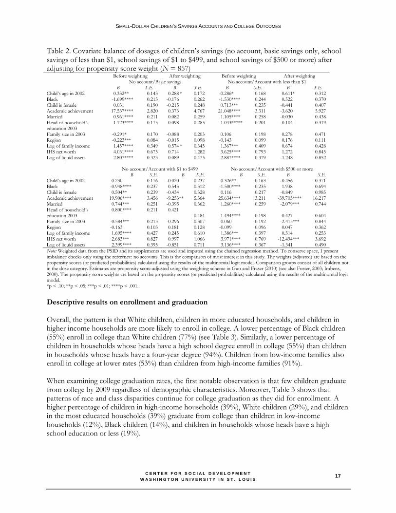
Results Findings from the covariate balance checks are discussed in the first part of this section, followed by logistic regression results for college enrollment and college graduation. However, only findings from propensity score adjusted models are discussed. Propensity score analysis allows researchers to balance potential bias between, for example, children exposed to having savings and those who are not, based on known covariates (Rosenbaum & Rubin, 1983). Until recently, propensity score methods have been limited to two-group situations, such as a single treatment and a comparison group. However, Imbens (2000) extends the method to multi-group situations (see Guo & Fraser, 2010). Because of selection effects in observational data, propensity score analysis is a more rigorous statistical strategy to estimate effects than a conventional regression or regression-type model. For this reason, I discuss findings from adjusted models only (Berk, 2004). Further, I report findings for controls only when using no savings as the reference group to save space because there are no meaningful differences when the reference group is changed among controls. Bivariate results from covariate balance checks Results from balance checks are presented in Table 2. In the unadjusted sample, almost all covariates show significant group differences regardless of the dosage. After propensity score weighting, group differences are no longer significant in almost all cases, which suggests that weighting is successful in reducing bias among observed covariates. For those with school savings of $500 or more, academic achievement, marital status, family size, and net worth remain significant, which suggests that attempting to generalize findings from results for children with $500 or more should be done with caution.



17

Table 2. Covariate balance of dosages of children’s savings (no account, basic savings only, school savings of less than $1, school savings of $1 to $499, and school savings of $500 or more) after adjusting for propensity score weight (N = 857) Before weighting After weighting Before weighting After weighting No account/Basic savings No account/Account with less than $1 B S.E. B S.E. B S.E. B S.E. Child’s age in 2002 0.332 ** 0.143 0.288 * 0.172 -0.286 * 0.168 0.611 * 0.312 Black -1.699 **** 0.213 -0.176 0.262 -1.530 **** 0.244 0.522 0.370 Child is female 0.031 0.190 -0.215 0.248 0.713 *** 0.235 -0.441 0.407 Academic achievement 17.537 **** 2.820 0.373 4.767 21.048 **** 3.311 -3.620 5.927 Married 0.961 **** 0.211 0.082 0.259 1.105 **** 0.258 -0.030 0.438 Head of household’s education 2003

1.123 **** 0.175 0.098 0.283 1.043 ***** 0.201 -0.104 0.319

Family size in 2003 -0.291 * 0.170 -0.088 0.203 0.106 0.198 0.278 0.471 Region -0.223 *** 0.084 -0.015 0.098 -0.143 0.099 0.176 0.111 Log of family income 1.457 **** 0.349 0.574 * 0.345 1.367 *** 0.409 0.674 0.428 IHS net worth 4.031 **** 0.675 0.714 1.282 3.625 **** 0.793 1.272 0.845 Log of liquid assets 2.807 **** 0.323 0.089 0.473 2.887 **** 0.379 -1.248 0.852

No account/Account with $1 to $499 No account/Account with $500 or more B S.E. B S.E. B S.E. B S.E. Child’s age in 2002 0.230 0.176 -0.020 0.237 0.326 ** 0.163 -0.456 0.371 Black -0.948 **** 0.237 0.543 0.312 -1.500 **** 0.235 1.938 0.694 Child is female 0.504 ** 0.239 -0.434 0.328 0.116 0.217 -0.849 0.985 Academic achievement 19.906 **** 3.456 -9.253 ** 5.364 25.634 **** 3.211 -39.703 **** 16.217 Married 0.744 *** 0.251 -0.395 0.362 1.260 **** 0.259 -2.079 *** 0.744 Head of household’s education 2003

0.800 **** 0.211 0.421 0.484 1.494 **** 0.198 0.427 0.604

Family size in 2003 -0.584 *** 0.213 -0.296 0.307 0.060 0.192 -2.415 *** 0.844 Region -0.163 0.103 0.181 0.128 -0.099 0.096 0.047 0.362 Log of family income 1.695 **** 0.427 0.245 0.610 1.386 *** 0.397 0.314 0.253 IHS net worth 2.683 *** 0.827 0.997 1.066 3.971 **** 0.769 -12.494 *** 3.692 Log of liquid assets 2.399 **** 0.395 -0.851 0.711 3.136 **** 0.367 -1.341 0.490

Note: Weighted data from the PSID and its supplements are used and imputed using the chained regression method. To conserve space, I present imbalance checks only using the reference: no accounts. This is the comparison of most interest in this study. The weights (adjusted) are based on the propensity scores (or predicted probabilities) calculated using the results of the multinomial logit model. Comparison groups consist of all children not in the dose category. Estimates are propensity score-adjusted using the weighting scheme in Guo and Fraser (2010) (see also Foster, 2003; Imbens, 2000). The propensity score weights are based on the propensity scores (or predicted probabilities) calculated using the results of the multinomial logit model. *p < .10; **p < .05; ***p < .01; ****p < .001.

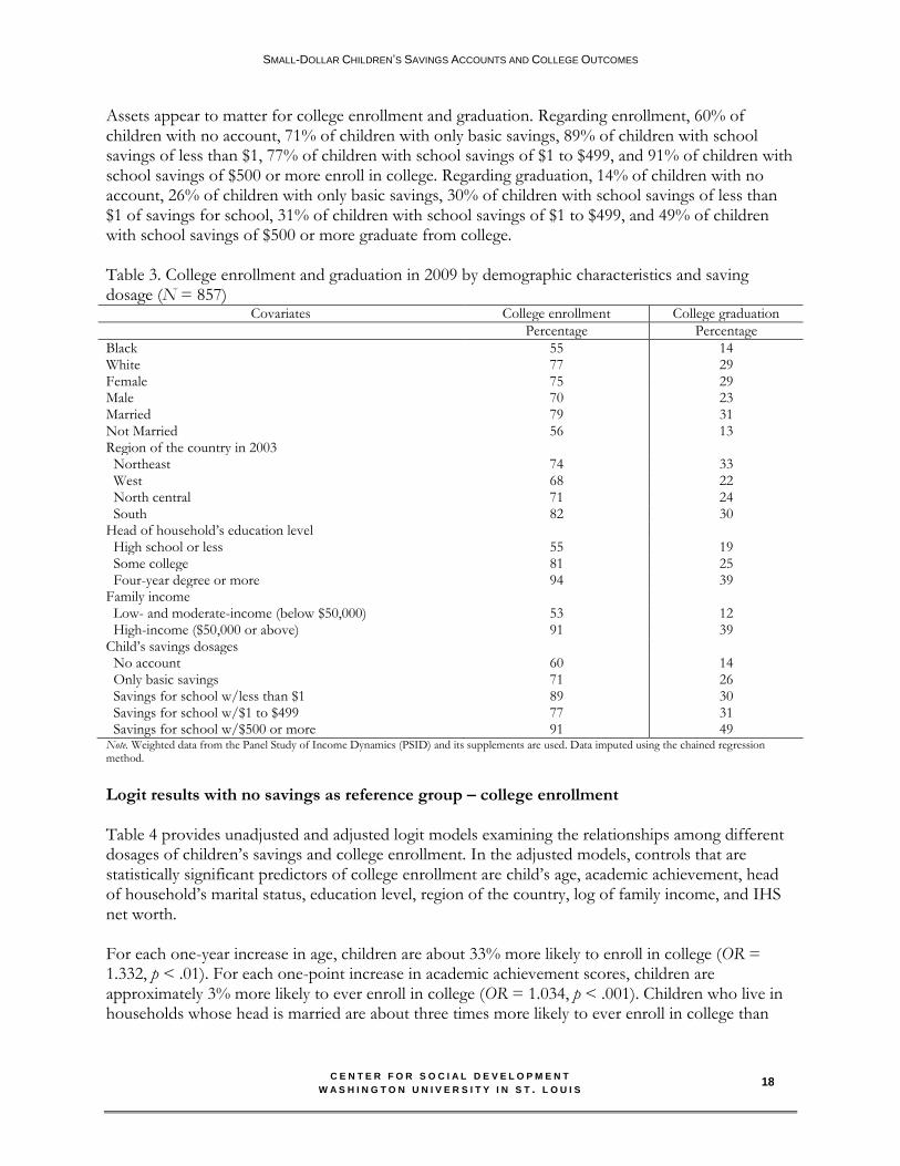
Descriptive results on enrollment and graduation Overall, the pattern is that White children, children in more educated households, and children in higher income households are more likely to enroll in college. A lower percentage of Black children (55%) enroll in college than White children (77%) (see Table 3). Similarly, a lower percentage of children in households whose heads have a high school degree enroll in college (55%) than children in households whose heads have a four-year degree (94%). Children from low-income families also enroll in college at lower rates (53%) than children from high-income families (91%). When examining college graduation rates, the first notable observation is that few children graduate from college by 2009 regardless of demographic characteristics. Moreover, Table 3 shows that patterns of race and class disparities continue for college graduation as they did for enrollment. A higher percentage of children in high-income households (39%), White children (29%), and children in the most educated households (39%) graduate from college than children in low-income households (12%), Black children (14%), and children in households whose heads have a high school education or less (19%).



18

Assets appear to matter for college enrollment and graduation. Regarding enrollment, 60% of children with no account, 71% of children with only basic savings, 89% of children with school savings of less than $1, 77% of children with school savings of $1 to $499, and 91% of children with school savings of $500 or more enroll in college. Regarding graduation, 14% of children with no account, 26% of children with only basic savings, 30% of children with school savings of less than $1 of savings for school, 31% of children with school savings of $1 to $499, and 49% of children with school savings of $500 or more graduate from college. Table 3. College enrollment and graduation in 2009 by demographic characteristics and saving dosage (N = 857)

Covariates College enrollment College graduation

Percentage Percentage

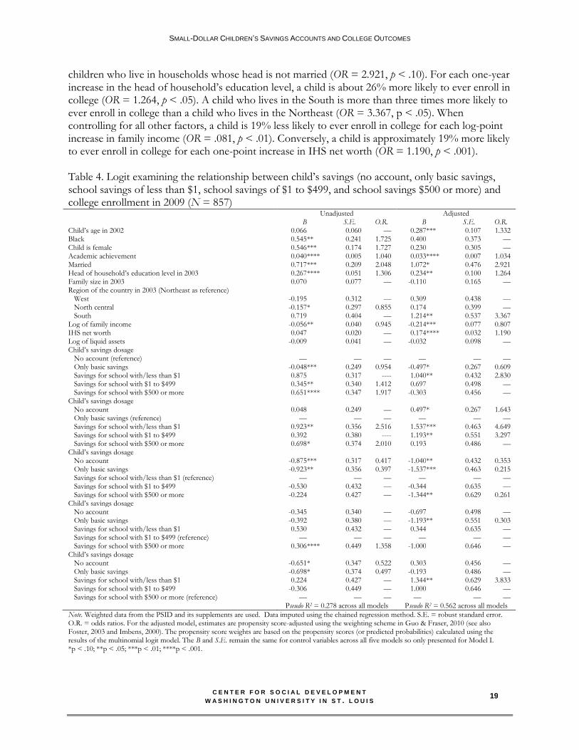
Black 55 14 White 77 29 Female 75 29 Male 70 23 Married 79 31 Not Married 56 13 Region of the country in 2003 Northeast 74 33 West 68 22 North central 71 24 South 82 30 Head of household’s education level High school or less 55 19 Some college 81 25 Four-year degree or more 94 39 Family income Low- and moderate-income (below $50,000) 53 12 High-income ($50,000 or above) 91 39 Child’s savings dosages No account 60 14 Only basic savings 71 26 Savings for school w/less than $1 89 30 Savings for school w/$1 to $499 77 31 Savings for school w/$500 or more 91 49 Note. Weighted data from the Panel Study of Income Dynamics (PSID) and its supplements are used. Data imputed using the chained regression method. Logit results with no savings as reference group – college enrollment Table 4 provides unadjusted and adjusted logit models examining the relationships among different dosages of children’s savings and college enrollment. In the adjusted models, controls that are statistically significant predictors of college enrollment are child’s age, academic achievement, head of household’s marital status, education level, region of the country, log of family income, and IHS net worth. For each one-year increase in age, children are about 33% more likely to enroll in college (OR = 1.332, p < .01). For each one-point increase in academic achievement scores, children are approximately 3% more likely to ever enroll in college (OR = 1.034, p < .001). Children who live in households whose head is married are about three times more likely to ever enroll in college than



19

children who live in households whose head is not married (OR = 2.921, p < .10). For each one-year increase in the head of household’s education level, a child is about 26% more likely to ever enroll in college (OR = 1.264, p < .05). A child who lives in the South is more than three times more likely to ever enroll in college than a child who lives in the Northeast (OR = 3.367, p < .05). When controlling for all other factors, a child is 19% less likely to ever enroll in college for each log-point increase in family income (OR = .081, p < .01). Conversely, a child is approximately 19% more likely to ever enroll in college for each one-point increase in IHS net worth (OR = 1.190, p < .001). Table 4. Logit examining the relationship between child’s savings (no account, only basic savings, school savings of less than $1, school savings of $1 to $499, and school savings $500 or more) and college enrollment in 2009 (N = 857) Unadjusted Adjusted B S.E. O.R. B S.E. O.R. Child’s age in 2002 0.066 0.060 — 0.287 *** 0.107 1.332 Black 0.545 ** 0.241 1.725 0.400 0.373 — Child is female 0.546 *** 0.174 1.727 0.230 0.305 — Academic achievement 0.040 **** 0.005 1.040 0.033 **** 0.007 1.034 Married 0.717 *** 0.209 2.048 1.072 * 0.476 2.921 Head of household’s education level in 2003 0.267 **** 0.051 1.306 0.234 ** 0.100 1.264 Family size in 2003 0.070 0.077 — -0.110 0.165 — Region of the country in 2003 (Northeast as reference) West -0.195 0.312 — 0.309 0.438 — North central -0.157 * 0.297 0.855 0.174 0.399 — South 0.719 0.404 — 1.214 ** 0.537 3.367 Log of family income -0.056 ** 0.040 0.945 -0.214 *** 0.077 0.807 IHS net worth 0.047 0.020 — 0.174 **** 0.032 1.190 Log of liquid assets -0.009 0.041 — -0.032 0.098 — Child’s savings dosage No account (reference) — — — — — — Only basic savings -0.048 *** 0.249 0.954 -0.497 * 0.267 0.609 Savings for school with/less than $1 0.875 0.317 ---- 1.040 ** 0.432 2.830 Savings for school with $1 to $499 0.345 ** 0.340 1.412 0.697 0.498 — Savings for school with $500 or more 0.651 **** 0.347 1.917 -0.303 0.456 — Child’s savings dosage No account 0.048 0.249 — 0.497 * 0.267 1.643 Only basic savings (reference) — — — — — — Savings for school with/less than $1 0.923 ** 0.356 2.516 1.537 *** 0.463 4.649 Savings for school with $1 to $499 0.392 0.380 ---- 1.193 ** 0.551 3.297 Savings for school with $500 or more 0.698 * 0.374 2.010 0.193 0.486 — Child’s savings dosage No account -0.875 *** 0.317 0.417 -1.040 ** 0.432 0.353 Only basic savings -0.923 ** 0.356 0.397 -1.537 *** 0.463 0.215 Savings for school with/less than $1 (reference) — — — — — — Savings for school with $1 to $499 -0.530 0.432 — -0.344 0.635 — Savings for school with $500 or more -0.224 0.427 — -1.344 ** 0.629 0.261 Child’s savings dosage No account -0.345 0.340 — -0.697 0.498 — Only basic savings -0.392 0.380 — -1.193 ** 0.551 0.303 Savings for school with/less than $1 0.530 0.432 — 0.344 0.635 — Savings for school with $1 to $499 (reference) — — — — — — Savings for school with $500 or more 0.306 **** 0.449 1.358 -1.000 0.646 — Child’s savings dosage No account -0.651 * 0.347 0.522 0.303 0.456 — Only basic savings -0.698 * 0.374 0.497 -0.193 0.486 — Savings for school with/less than $1 0.224 0.427 — 1.344 ** 0.629 3.833 Savings for school with $1 to $499 -0.306 0.449 — 1.000 0.646 — Savings for school with $500 or more (reference) — — — — — — Pseudo R2 = 0.278 across all models Pseudo R2 = 0.562 across all models

Note. Weighted data from the PSID and its supplements are used. Data imputed using the chained regression method. S.E. = robust standard error. O.R. = odds ratios. For the adjusted model, estimates are propensity score-adjusted using the weighting scheme in Guo & Fraser, 2010 (see also Foster, 2003 and Imbens, 2000). The propensity score weights are based on the propensity scores (or predicted probabilities) calculated using the results of the multinomial logit model. The B and S.E. remain the same for control variables across all five models so only presented for Model I. *p < .10; **p < .05; ***p < .01; ****p < .001.



20

Among variables of interest, having basic savings is negatively associated with college enrollment, while having school savings of less than $1 is a statistically significant predictor of college enrollment in the adjusted model. A child with basic savings prior to reaching college age is 39% less likely to ever enroll in college than a child with no savings prior to reaching college age (OR = .609, p < .10). A child with less than $1 designated savings for school is about three times more likely to ever enroll in college than a child with no savings (OR = 2.830, p < .05). Dosage-specific findings – college enrollment Findings indicate that children with no savings accounts, savings for school of less than $1, or savings for school of $1 to $499 are more likely to ever enroll in college by 2009 than children with only basic savings (see Table 4). Children with no savings are about 64% more likely to ever enroll in college than children with basic savings only (OR = 1.643, p < .10). Children with school savings of less than $1 are more than four and half times more likely to ever enroll in college than children with basic savings only (OR = 4.649, p < .01). Children with school savings of $1 to $499 are more than three times more likely to ever enroll in college than children with basic savings only (OR = 3.297, p < .05). The following dosages are statistically significant when children with school savings of less than $1 are used as the reference group: those with no account, those with basic savings only, and those with school savings of $500 or more. Children with no accounts are nearly 65% less likely to ever enroll in college than children with school savings of less than $1 (OR = 0.353, p < .05). Children with basic savings only are 79% less likely to ever enroll in college than children with school savings of less than $1 (OR = 0.215, p < .01). Children with school savings of $500 or more are almost 74% less likely to ever enroll in college than children with school savings of less than $1 (OR = 0.261, p < .05). The only significant dosage when children with school savings of $1 to $499 are used as the reference group is basic savings only. Children with basic savings are about 70% less likely to ever enroll in college than children with school savings of $1to $499 (OR = 0.303, p < .05). In the final college enrollment model, I find that the school savings of less than $1 dosage is a statistically significant predictor of college enrollment when children with school savings of $500 or more are used as the reference group. Children with school savings of less than $1 are almost four times more likely to ever enroll in college than children with school savings of $500 or more (OR = 3.833, p < .05). Logit results with no savings as reference group – college graduation Table 5 provides information on two-year or four-year college graduation. In the adjusted models, controls that are statistically significant predictors of college enrollment are child’s age, gender, academic achievement, log of family income, and IHS net worth.

For each one-year increase in age, a child is about 39% less likely to graduate from college (OR = 1.610, p < .001). Female children are about 64% more likely than male children to graduate from college after controlling for all other factors (OR = 1.635, p < .10). For each one-point increase in a child’s academic achievement score, the child is approximately 1% more likely to graduate from college (OR = 1.012, p < .10). For each log-point increase in family income, a child is 26% less likely



21

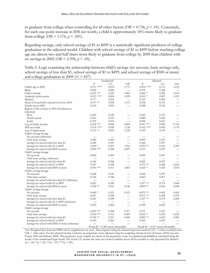
to graduate from college when controlling for all other factors (OR = 0.736, p < .01). Conversely, for each one-point increase in IHS net worth, a child is approximately 18% more likely to graduate from college (OR = 1.176, p < .001). Regarding savings, only school savings of $1 to $499 is a statistically significant predictor of college graduation in the adjusted model. Children with school savings of $1 to $499 before reaching college age are almost two and half times more likely to graduate from college by 2009 than children with no savings in 2002 (OR = 2.394, p < .05).

Table 5. Logit examining the relationship between child’s savings (no account, basic savings only, school savings of less than $1, school savings of $1 to $499, and school savings of $500 or more) and college graduation in 2009 (N = 857) Unadjusted Adjusted B S.E. O.R. B S.E. O.R. Child’s age in 2002 0.571 **** 0.074 1.771 0.476 **** 0.112 1.610 Black -0.092 0.282 — -0.476 0.368 — Child is female 0.623 *** 0.210 1.865 0.492 * 0.296 1.635 Academic achievement 0.019 **** 0.004 1.020 0.012 * 0.007 1.012 Married 0.177 0.264 — -0.155 0.404 — Head of household’s education level in 2003 0.107 ** 0.054 1.113 0.238 0.151 — Family size in 2003 0.103 0.093 — 0.028 0.126 — Region of the country in 2003 (Northeast as reference)

West -0.422 0.320 — -0.249 0.370 — North central -0.261 0.319 — 0.089 0.382 — South -0.195 0.355 — -0.094 0.415 — Log of family income -0.218 *** 0.068 0.804 -0.307 *** 0.090 0.736 IHS net worth 0.114 **** 0.030 1.120 0.162 **** 0.045 1.176 Log of liquid assets 0.115 ** 0.055 1.122 0.102 0.105 — Child’s savings dosage No account (reference) — — — — — — Only basic savings 0.082 0.304 — -0.099 0.307 — Savings for school with/less than $1 0.228 0.341 — -0.364 0.397 — Savings for school with $1 to $499 0.649 * 0.351 1.914 0.873 ** 0.432 2.394 Savings for school with $500 or more 0.992 *** 0.308 2.697 0.531 0.327 — Child’s savings dosage No account -0.082 0.304 — 0.099 0.307 — Only basic savings (reference) — — — — — — Savings for school with/less than $1 0.146 0.346 — -0.265 0.407 — Savings for school with $1 to $499 0.567 0.358 — 0.972 ** 0.428 2.643 Savings for school with $500 or more 0.910 *** 0.311 2.483 0.630 * 0.343 1.878 Child’s savings dosage No account -0.228 0.341 — 0.364 0.397 — Only basic savings -0.146 0.346 — 0.265 0.407 — Savings for school with/less than $1 (reference) — — — — — — Savings for school with $1 to $499 0.421 0.389 — 1.237 ** 0.574 3.444 Savings for school with $500 or more 0.764 ** 0.351 2.146 0.895 ** 0.432 2.448 Child’s savings dosage No account -0.649 * 0.351 0.523 -0.873 ** 0.432 0.418 Only basic savings -0.567 0.358 — -0.972 ** 0.428 0.378 Savings for school with/less than $1 -0.421 0.389 — -1.237 ** 0.574 0.290 Savings for school with $1 to $499 (reference) — — — — — — Savings for school with $500 or more 0.343 0.362 — -0.342 0.453 — Child’s savings dosage No account -0.992 *** 0.308 0.371 -0.531 0.327 — Only basic savings -0.910 *** 0.311 0.403 -0.630 * 0.343 0.532 Savings for school with/less than $1 -0.764 ** 0.351 0.466 -0.895 ** 0.432 0.409 Savings for school with $1 to $499 -0.343 0.362 — 0.342 0.453 — Savings for school with $500 or more (reference) — — — — — — Pseudo R2 = 0.261 across all models Pseudo R2 = 0.317 across all models

Note. Weighted data from the PSID and its supplements are used. Data imputed using the chained regression method. S.E. = robust standard error. O.R. = odds ratios. For the adjusted model, estimates are propensity score-adjusted using the weighting scheme in Guo & Fraser (2010) (see also Foster, 2003 and Imbens, 2000). The propensity score weights are based on the propensity scores (or predicted probabilities) calculated using the results of the multinomial logit model. The B and S.E. remain the same for control variables across all five models so only presented for Model I. *p < .10; **p < .05; ***p < .01; ****p < .001.



22

Dosage specific findings – college graduation Findings indicate that children with school savings of $1 to $499 or $500 or more are more likely to graduate from college than children with basic savings only (see Table 5). Children with $1 to $499 are about two and half times more likely to graduate from college than children with basic savings only (OR = 2.643, p < .05). Children with school savings of $500 or more are about twice as likely to graduate from college than children with basic savings only (OR = 1.878, p < .10). The following dosages are statistically significant when children with school savings of less than $1 are used as the reference group: school savings of $1 to $499 and school savings of $500 or more. Children with school savings of $1 to $499 are about three and half times more likely to graduate from college than children with school savings of less than $1 (OR = 3.444, p < .05). Children with school savings of $500 or more are almost two and half times more likely to graduate from college than children with school saving of less than $1 (OR = 2.448, p < .05). Having no account, basic savings only, or savings for school of less than $1 are significant when children with school savings of $1 to $499 are used as the reference group. Children with no account are 59% less likely to graduate from college than children with school savings of $1 to $499 (OR = 0.418, p < .05). Children with basic savings only are about 62% less likely to graduate from college than children with school savings of $1 to $499 (OR = 0.378, p < .05). Children with school savings of less than $1 are about 71% less likely to graduate from college than children with school savings of $1 to $499 (OR = 0.290, p < .05). In the final college graduation model, I find having basic savings only or school savings of less than $1 are statistically significant predictors of college graduation when children with school savings of $500 or more are used as the reference group. Children with basic savings only are almost 47% less likely to graduate college than children with school savings of $500 or more (OR = 0.532, p < .10). Children with school savings of less than $1 are almost 59% less likely to graduate college than children with school savings of $500 or more (OR = 0.409, p < .05).

Discussion The DOE’s announcement of a new college savings account research demonstration project to be implemented within the GEAR UP program has raised questions about whether small-dollar savings accounts can improve college enrollment and graduation rates. This study examines whether children’s savings are associated with college graduation, small-dollar accounts can have a positive effect on children’s educational outcomes, and having savings specifically designated for school is a stronger predictor of children’s college outcomes than having basic savings only. Consistent with previous research (e.g., Elliott & Beverly, 2011a), findings suggest that having savings is an important predictor of college enrollment. However, this paper improves upon past research by using propensity score weighting, which allows researchers to balance potential bias between children exposed to having savings and those who are not, based on known covariates (Rosenbaum & Rubin, 1983). This study also improves upon past research by measuring dosages of children’s savings (no savings, basic savings only, and school savings of less than $1, $1 to $499, and



23

$500 or more). By doing so, I examine whether different amounts of savings—particularly small-dollar amounts—can have a positive effect on children’s college enrollment outcomes. Regarding college enrollment, findings suggest that children who have basic savings only are less likely to enroll in college than children with no savings at all. Elliott, Chowa, and Loke (2011) also find that having basic savings only is a negative predictor of college enrollment, possibly because children with basic savings who do not designate some of it for college are less likely to see college as an important or attainable goal. This implies that most children who have savings and perceive of college as important designate some of that savings for college even if they do not save large amounts. Elliott, Chowa, and Loke (2011) find that children who expect to graduate from college and have basic savings are more likely to enroll in college than children with no savings, children who expect to graduate but have no savings, and children with basic savings who do not expect to graduate. Findings from this study also indicate that having school savings of $1 or less increases the odds that a child enrolls in college. While this finding suggests that even very small-dollar amounts can make a difference in whether a child enrolls in college, the fact that having larger amounts is not significant raises questions about why small-dollar amounts do and larger dollar amounts do not. Having larger amounts may not be significant because children with higher amounts of savings might also have other characteristics (e.g., being high academic achievers) or external circumstances (e.g., having parents who have attended college or are high-income) that make them likely to attend college, reducing the overall effect of having savings. Elliott, Constance-Huggins, and Song (2012) use separate samples of low-income and high-income children and find that having school savings is significantly related to college progress (i.e., being currently enrolled in college or having graduated from college) among low-income but not high-income children. Propensity score-weighted balance checks for this study also suggest that this might be the case, particularly among children with school savings of $500 or more. Even with weighting, academic achievement, head of household’s education level, family size, and family net worth remain significant predictors of having school savings of $500 or more and are important predictors of college enrollment in previous studies. While it is not particularly surprising to find that children from more advantaged backgrounds are disproportionately represented among children who have higher amounts of school savings, it is noteworthy that when children with similar observables (e.g., live in households with similar incomes, have parents with similar education levels, and have similar levels of academic achievement) are examined, those who have a small-dollar school accounts are more likely to enroll in college than those with no accounts. Overall, these findings can be interpreted as evidence for the proposition that small-dollar school savings accounts can play an important role in increasing children’s access to college. Further, when basic school savings and school savings of less than $1 are analyzed together, findings suggest that school savings are more likely than basic savings to positively affect children’s college enrollment. However, there is more direct evidence that having savings specifically for school is a stronger predictor of children’s college outcomes than having basic savings only. When basic savings is used as the reference group, having less than $1 of school savings and having $1 to $499 of school savings are both positive predictors of college enrollment.



24

Even after controlling for children’s savings, academic achievement, marital status, and head of household’s education level remain consistent positive predictors of college enrollment. Previous research on net worth and college enrollment that controls for academic achievement has been mixed,12 but in this study, I find that net worth is a significant predictor of college enrollment. An important difference between this study and previous research is the way net worth is measured. In this study, I use the inverse hyperbolic sine (IHS) of net worth instead of the natural log of net worth, the benefits of which are that IHS allows for the existence of negative values and can more clearly demonstrate changes in the wealth distribution (Kennickell & Woodburn, 1999), whereas the natural log transformation does not. Interestingly, income is a negative predictor of college enrollment. That is, after controlling for all other factors, higher income children are actually less likely to enroll in college by 2009. This might be because of the way that college enrollment is measured. College enrollment includes two- and four-year college attendance, and in this sample, more children attend two-year colleges than four-year colleges. Further, research suggests that lower income children are more likely to enroll in two-year than four-year colleges (Louie, 2007). Given this imbalance, the result might be driven primarily by two-year college enrollment. The same might be true for college graduation because income is also a negative predictor of college graduation. Regarding college graduation, I find that having small-dollar accounts is statistically significant. However, children with less than $1 of school savings are not significantly more likely to graduate from college than children who have no savings, but children with $1 to $499 of savings are more likely to graduate from college than children with no savings. Practically speaking, it might not matter whether children have less than $1 or $1 to $499 since neither is enough savings to pay for a single credit hour or books for one semester at most colleges. I suggest that the effects from small-dollar accounts are not based primarily on helping children pay for college but rather on the psychological effects and resultant behavioral changes. From an IBM perspective, designating money for college involves thinking actively about college and saving (i.e., identity salience), understanding that others who are similar go to college (i.e., group congruence), and viewing college as an important goal and saving as a way to pay for it (i.e., interpretation of difficulty as normal). According to IBM theory, salience, group congruence, interpretation of difficulty as normal, are important predictors of school engagement. In turn, school engagement has been linked to positive educational outcomes (e.g., Oyserman & Destin, 2010).

Limitations Propensity score analyses have two clear disadvantages relative to randomized trials. One is the need to assume conditional independence (i.e., eliminate selection bias by controlling for observed covariates). This may not be true as it is impossible to know all the covariates that may influence the choice to participate in treatment. The precision of controlling for treatment choice goes as far as the covariates included in the study. In randomized trials, the researcher can be confident that the treatment group and the control group are similar in observed and unobserved characteristics.

12 For a review of these studies, see Elliott, Destin, & Friedline (2011).



25

Second, whereas propensity score analyses can estimate treatment effects only where there is overlap between the exposed group (e.g., that does have savings) and the unexposed group (e.g., that does not have savings), random assignment ensures that there is common support across the entire sample. These considerations make experimental techniques superior to propensity score analyses in a number of important ways. However, randomization also has limitations of cost and time. Cost is a major concern when designing random control trials to test CDAs because providing children with initial deposits and savings matches is expensive. A large experiment called SEED for Oklahoma Kids (SEED OK) with CDAs in the state’s name and youth as beneficiaries is being tested.13 However, because the accounts were issued at birth in 2004, researchers will not be able to test this design as it relates to college progress for a number of years. In the meantime, CDAs have been proposed in Congress, and providing policymakers with information and using the best available data and methodology are of the utmost importance. Another limitation of this study is the lack of variation in school savings amount. Few children have savings above $1,000. Given this, it is hard to examine at what exact point the amount of savings matters, particularly at the high end. Ideally, researchers would be able to examine a number of different cut points, but the primary question in this study is whether or not small-dollar accounts matter for improving children’s college enrollment and graduation rates. It is also important to point out that propensity score weights are less effective for school savings of $500 or more. After weighting, academic achievement, head of household’s education level, family size, and family net worth remain significant. Given this, results for school savings of $500 or more should be interpreted with caution.

Policy Implications The results from this study indicate that policies for building children’s wealth as a way to improve college enrollment and graduation might still have positive effects even when children mentally designate relatively small amounts of savings for school. Further, when examining whether a school savings program is effective, these findings suggest that savings behaviors or amounts saved might not be the best indicator. Instead, children’s improvement in school (e.g., academic achievement scores, college enrollment rates, and college graduation rates) might be a better or at least equally important indicator. Findings also imply that children’s savings programs that have raising college enrollment and graduation rates as their primary goal might be more successful if they either create a separate account for school purposes or encourage children to designate a portion of their savings specifically for school purposes. Encouraging this type of savings might be done as part of a financial literacy class or as a financial literacy component of a children’s savings program.

Conclusion This study provides some evidence that designating money for college through a mental accounting process can have a positive effect on college enrollment and graduation even when small amounts are allocated for school. However, because of their inability to process all cognitive stimuli and limited capacity for making conscious decisions (i.e., Bargh & Chartrand, 1999), children may be

13 For more information on SEED OK, see http://csd.wustl.edu/AssetBuilding/SEEDOK.

http://csd.wustl.edu/AssetBuilding/SEEDOK



26

unlikely to form mental accounts via conscious processes. Further, children who subsist at the level of meeting basic survival needs only may not be likely to develop strategies for financing college, even if the desire to attend is there. Formal institutions may be able to provide children with schemas, rules, norms, and routines that become embedded thought processes and can be used to develop an identity as a college saver. According to Sherraden and Barr (2005), a formal institution within the applied social science context can be thought of as at type of intervention designed to alter behaviors and outcomes of individuals (i.e., institutional theory). As such, a national children’s savings program might be thought of as a type of institution designed to help children form college-saver identities (i.e., college savings programs may encourage children to adopt future-oriented or asset-based patterns of behavior). In an analysis of institutions and rational choice, Nobel Prize winner Douglas North (2005) states, ―…much of what passes for rational choice is not so much individual cogitation as the embeddedness of the thought process in the larger social and institutional context‖ (p. 24). Similarly, in reference to asset accumulation, Michael Sherraden (1991) observes that the middle-class, ―participates in retirement pension systems…not [as] a matter of making superior choices. Instead, a priori choices are made by social policy, and individuals walk into the pattern that has been established‖ (p. 127). If we agree with these views, children’s savings programs hold real promise for helping children not only pay for education but also develop mental accounting strategies that might lead to the development of a college-saver identity and greater engagement in school. However, more research is needed.



27

References Advisory Committee on Student Financial Assistance (ACSFA). (2001). Access denied: Restoring the

nation’s commitment to equal educational opportunity. Retrieved from http://www2.ed.gov/about/bdscomm/list/acsfa/access_denied.pdf

Advisory Committee on Student Financial Assistance (ACSFA). (2006). Mortgaging our future: How financial barriers to college undercut America’s global competitiveness (pp. 1–63). Washington, DC: Advisory Committee on Student Financial Assistance.

Baily, M., & Dynarski, S. (2011). Gains and gaps: Changing inequality in U.S. college entry and completion (Working Paper 17633). Cambridge, MA: National Bureau of Economic Research (NBER).

Bargh, J., & Chartrand, T. (1999). The unbearable automaticity of being. American Psychologist, 54(7), 462–479.

Baum, S., & Steele, P. (2010). Who borrows most? Bachelor’s degree recipients with high levels of student debt. Retrieved from http://advocacy.collegeboard.org/sites/default/files/Trends-Who-Borrows-Most-Brief.pdf

Berk, R. A. (2004). Regression analysis: A constructive critique. Thousand Oaks, CA: Sage Publications. Cramer, R. (2010). The big lift: Federal policy efforts to create child development accounts. Children

and Youth Services Review, 32(11), 1538–1543. Cramer, R., & Newville, D. (2009, December). Children’s Savings Accounts: The case for creating a lifelong

savings platform at birth as a foundation for a “save-and-invest” economy. Washington, DC: New American Foundation.

Elliott, W. (2013). The effects of economic instability on children’s educational outcomes. Children and Youth Services Review, 35(3), 461–471. doi:10.1016/j.childyouth.2012.12.017

Elliott, W., & Beverly, S. (2011a). Staying on course: The effects of assets and savings on the college progress of young adults. American Journal of Education, 117(3), 343–374.

Elliott, W., & Beverly, S. (2011b). The role of savings and wealth in reducing ―wilt‖ between expectations and college attendance. Journal of Children and Poverty, 17(2), 165–185.

Elliott, W., Choi, E. H., Destin, M., & Kim, K. (2011). The age old question, which comes first? A simultaneous test of children’s savings and children’s college-bound identity. Children and Youth Services Review, 33(7), 1101–1111.

Elliott, W., Chowa, G., & Loke, V. (2011). Toward a children’s savings and college-bound identity intervention for raising college attendance rates: A multilevel propensity score analysis. Sociology Mind, 1(4), 192–205.

Elliott, W., Constance-Huggins, M., & Song, H. (2012). Improving college progress among low- to moderate-income (LMI) young adults: The role of assets. Journal of Family and Economic Issues. doi:10.1007/s10834-012-9341-0

Elliott, W., Destin, M., & Friedline, T. (2011). Taking stock of ten years of research on the relationship between assets and children’s educational outcomes: Implications for theory, policy, and intervention. Children and Youth Services Review, 33(11), 2312–2328.

Elliott, W. & Friedline, T. (2012). ―You pay your share, we’ll pay our share‖: The college cost burden and the role of race, income, and college assets. Economics of Education Review. Advance online publication. doi:10.1016/j.econedurev.2012.10.001

Elliott, W., Jung, H., & Friedline, T. (2011). Raising math scores among children in low-wealth households: Potential benefit of children’s school savings. Journal of Income Distribution, 20(2), 72–91.

Elliott, W., & Nam, I. (2012). Direct effects of assets and savings on the college progress of Black young adults. Educational Evaluation and Policy Analysis, 34(1), 89–108.

http://www2.ed.gov/about/bdscomm/list/acsfa/access_denied.pdf

http://advocacy.collegeboard.org/sites/default/files/Trends-Who-Borrows-Most-Brief.pdf

http://advocacy.collegeboard.org/sites/default/files/Trends-Who-Borrows-Most-Brief.pdf



28

Elliott, W., Sherraden, M., Johnson, L., & Guo, B. (2010). Young children’s perceptions of college and saving: The potential role of child development accounts. Children and Youth Services Review, 32(11), 1577–1584.

Entwisle, D. R., Alexander, K. L., & Olson, L. S. (2005). First grade and educational attainment by age 22: A new story. American Journal of Sociology, 110(5), 1458–1502.

Foster, M. E. (2003). Propensity score matching: An illustrative analysis of dose response. Medical Care, 41(10), 1183–1192.

Graham, J. W., Taylor, B. J., & Cumsille, P. E. (2001). Planned missing data designs in analysis of change. In L. M. Collins & A. Sayer (Eds.), New methods for the analysis of change: vol. 1 (pp. 335–353). Washington, DC: American Psychological Association.

Guo, S., & Fraser, W. M. (2010). Propensity score analysis: Statistical methods and applications. Thousand Oaks, CA: Sage Publications.

Imbens, G. W. (2000). The role of the propensity score in estimating dose-response functions. Biometrika, 87(3), 706–710.

Jackson, G. A. (1978). Financial aid and student enrollment. Journal of Higher Education, 49(6), 548–574.

Kahneman, D., & Tversky, A. (1979). Prospect theory: An analysis of decision under risk. Econometrica, 47(2), 263-292.

Kennickell, A. B., & Woodburn, R. L. (1999). Consistent weight design for the 1989, 1992, and 1995 SCFs, and the distribution of wealth. Review of Income and Wealth, 45(2), 193–215. doi:10.1111/j.1475-4991.1999.tb00328.x

Kornrich, S., & Furstenberg, F. (2010). Investing in children: Changes in parental spending on children, 1972 to 2007. University of Sydney: The United States Studies Center.

Lea, S. E. G., Tarpy, R. M., & Webley, P. (1987). The individual in the economy. Cambridge, MA: Cambridge University Press.

Loke, V., & Sherraden, M. (2009). Building assets from birth: A global comparison of child development account policies. International Journal of Social Welfare, 18(2), 119–129.

Louie, V. (2007). Who makes the transition to college? Why we should care, what we know, and what we need to do. Teachers College Record, 109(10), 2222–2251.

Mainieri, T. (2006). The Panel Study of Income Dynamics Child Development Supplement: User guide for CDS-II. Ann Arbor, MI: University of Michigan, Institute for Social Research.

Nam, Y., Kim, Y., Clancy, M., Zager, R., & Sherraden, M. (2011). Do Child Development Accounts promote account holding, saving, and asset accumulation for children’s future? Evidence from a statewide randomized experiment (CSD Working Paper 11-33). St. Louis, MO: Washington University, Center for Social Development.

Oyserman, D., & Destin, M. (2010). Identity-based motivation: Implications for intervention. The Counseling Psychologist, 38(7), 1001–1043.

R Development Core Team (2008). R: A language and environment for statistical computing. Vienna, Austria: R Foundation for Statistical Computing. Retrieved from http://www.R-project.org

Rosenbaum, P. R., & Rubin, D. B. (1983). The central role of the propensity score in observational studies for causal effects. Biometrika, 70(1), 41–55. doi:10.2307/2335942

Shafer, J. L. (1997). Analysis of Incomplete Multivariate Data. London, England: Chapman & Hall. Sherraden, M. (1991). Assets and the poor: A new American welfare policy. Armonk, NY: M.E. Sharpe. Sherraden, M., & Barr, M. (2005). Institutions and inclusion in saving policy. In N. P. Retsinas & E.

S. Belsky (Eds.), Building assets, building wealth: Creating wealth in low-income communities (pp. 286–315). Washington DC: Brookings Institution Press.

http://www.r-project.org/



29

Somers, P. & Cofer, J. (2000). Mortgaging the future: Student debt load in the U.S. Washington, DC: U.S. Senate Committee on Homeland Security & Governmental Affairs.

Thaler, R. H. (1985). Mental accounting and consumer choice. Marketing Science, 4(3), 199–214. Winnett, A., & Lewis, A. (1995). Household accounts, mental accounts, and savings behavior: Some

old economics rediscovered? Journal of Economic Psychology, 16(1995), 431–448. Xiao, J. J., & Anderson, J. G. (1997). Hierarchical financial needs reflected by household financial

asset shares. Journal of Family and Economic Issues, 18(4), 333–355. Xiao, J. J., & Noring, F. E. (1994). Perceive saving motives and hierarchical financial needs. Financial

Counseling and Planning, 5, 25–45. Recommended citation Elliott, W. (2012). Small-dollar children’s savings accounts and college outcomes (CSD Working Paper 13-05). St. Louis, MO: Washington University, Center for Social Development.

small-dollar children’s savings accounts and...

Documents