sliding observer-based feedback control for flexible joints manipulator

Automatica, Vol. 32, No. 9, pp. 124.%1254, 1996 Copyright @ 19% Elsevier Science Ltd

Printed in Great Britain. All rights reserved

PII: SOOOS-1098(96)00069-6 C005-lO9W6 $15.00+0.00

Sliding Observer-based Feedback Control for Flexible Joints Manipulator

JACQUES HERNANDEZ t and JEAN-PIERRE BARBOT *

A singular perturbation approach for trajectory tracking control combined with nonlinear sliding state observer is proposed in this paper. The stability of the closed-loop system is investigated. Key Words- Sliding observer; singular perturbation; flexible joints manipulator; nonlinear feedback control; closed-loop stability.

Abstract- High-precision measurements of joint displace- ments and elastic forces are available on a flexible joints manipulator. In contrast, velocity measurements and elastic forces derivative are, in many cases, contaminated by noise or unavailable (technical or economical constraint). It is, therefore, interesting to investigate the possibility of controi- Iing robot dynamics by only using position and elastic force measurements. This paper presents a singular perturbation approach for trajectory tracking control combined with nonlinear sliding state observer. The stability of the closed-loop system is investigated. Copyright @I996 Elsevier Science Ltd.

1. INTRODUCTION

The aim of this paper is to design, through singular perturbation methods, a nonlinear observer- based feedback control law, for tracking desired time-varying joint-space trajectories for flexible manipulators. It is well-known that these methods allow us to deal with models of reduced dimen- sions (slow and fast), and consequently simplify the control scheme. Such a type of manipulator admits a singularly perturbed model rewriting the Lagrangian model with a standard coordinates change (Barbot ef al., 1992; Kokotovic et al., 1986; Marino and Kokotovic, 1986; Sharkey and O’Reilly, 1988; Spong et al., 1987). Slow and fast variables are usually represented by the link positions and velocities on the one hand, and the elastic forces and their time derivatives on the

Received 1 November 1993; revised 10 May 1995; received in final form 10 January 1996. This paper was not presented at any IFAC meeting. This paper was recommended for publication in revised form by Associate Editor Y. Utkin under the direction of Editor Ruth F. Curtain. Corresponding author Dr Jean- Pierre Barbot. Tel. +33 1 69 85 17 45; Fax +33 1 69 41 30 60; E-mail [email protected]. + Laboratoire d’Automatique des Arts et Metiers, EN- SAM/CNAM, 21 rue Pine& 75013 Paris, France. * Laboratoire de Signaux & Systemes, CNRS!ESE, Plateau de Moulon, 91192 Gif sur Yvette Cedex, France.

other hand. A state observer is necessary since only joint positions *and elastic forces are mesured. Link velocities and elastic force time derivatives are generally not easily available due to technical or economical constraints, or they are highly contaminated by noise.

An n-degree-of-freedom flexible joints manipulator model can be rewritten in the following singular perturbation state-space form:

f = f(x1, x2, Zl),

c : b. = gh, x2, ~1, ~2, E) + bu, I- -I

y= 2: I I I L J

where x = [ti,, d21f E Rzn the slow variable vector represents link positions and velocities, z = [z’,, 41’ E R2” the fast variable vector represents elastic forces and their time derivatives. The ap- plied input torque is u E R” and b E lRhxn is a constant matrix. The mesurable state vector y E R2” represents the link positions and the elastic forces. The vector fields f(xr, x2, zi) E Rzn and g(xi, x2, zr, ~2, E) E R2” are nonlinear functions of the full state [x’, 2’1’.

Joint-space trajectories are represented by the vector x. Hence, from the availability of the link positions and the elastic forces through the output vector y, the goal is to find a nonlinear state observer C, and a control law u depending on the observed variables 22 and g2, the mesurable output vector y, and the desired time-varying trajectories vector xd, such that the augmented system (C, C,) asymptotically tracks xd.

Several alternative methods exist in the liter- ature for the design of different observer struc- tures: linearization by a change of coordinates and output injection (Bestle and Zeitz, 1983; Isidori, 1989; Krener and Isidori, 1983; Krener and Re-

1243

1244 J. Hernandez and J.-I? Barbot

spondek, 1985; Xia and Gao, 1988; Zeitz, 1987), variable structure systems (Canudas de Wit and Slotine, 1991; Slotine et al., 1986), Lyapunov-based design (Thau, 1973) high-gain design (Nicosia and Tornambe, 1989). However, closed-loop stabi!ity cannot be guaranteed a priori if the control design is based on the separation principle, which is verified only for linear systems (Luenberger, 1971).

The observer introduced in this paper is a sliding observer, which is deduced from the one proposed by Canudas de Wit and Slotine (199 1) for rigid manipulators. In the case of rigid manipulators some physical robot properties are explicitly exploited to show exponential convergence of the observation error vector. Here, in the case of flexible manipulators, it is still possible to use these properties. Sliding observers derive from a transposition of the switching controllers (Utkin, 1992) to the problem of state observation in nonlinear systems. Sliding control design consists in defining a switching surface in the phase plane which is rendered attractive by the action of the switching terms. The dynamics on the switching surface are determined by the Fillipov solution concept (Fillipov, 1960), which indicates that the system dynamic behaviour within the switching surface can be formally described as a pondered average combination of the dynamics of each side of the discontinuous surface. As usual, denoting as x^i, $*,I$ and $, the observations of x1, ~2, z1 and 22, respectively; Z, the observer model, is a copy of C including switching gains

c, :

x” = f(x,, 22, z,) + AI,,

EZ” = g(xl, &, ZI, %, E) -I- bu + I’&,

jT= ;; ) I 1 L _I

where j; = [q, g21f, 2 = I??,, ;‘;I’, A and T E lRgznxzn represent the observer gains, and the switching vector Is E lR2” is the following: I, = sign(y - 7). The vector y -y^ characterizes the mismatch between the measured vector y and its estimate j? The switching surface will be defined as y - y^ = 0.

The main drawback of the sliding techniques is a chattering motion generation on the switching surface. Chattering is unsuitable because it adds an important amount of high-frequency components to the control law which has discontinuities. How- ever chattering can be reduced by replacing the discontinuous switching functions by introducing suitable saturation functions. Asymptotic stability is lost and substituted by a practical stability concept; the error does not tend to zero but to a closed region around it, in a finite time.

Since for nonlinear systems, the separation principle is not verified, the authors (Djemai et al., 1993; Hernandez and Barbot, 1993) propose the follow-

ing approach. Consider the system C, in which the vector [?, 11’ is available by direct computation together with y = [x’,, 41’ obtained by direct measurement. The basic idea stands in designing the control law u as u = ~(2, 2, y, xd), which allows us to track asymptotically x^ to xd. Hence, the stability to zero of the observation error system C,, = C - CO, obtained with an adequate choice for the observer gains, allows us to conclude that x goes to xd. In other words, the augmented system (Z, 1,) is ‘equivalent’ to the augmented system (C,, C,,). The closed-loop stability of (Co, C,,) is obtained by means of a singular perturbation technique. For an other approach, in the case of rigid joints manipulator, see Canudas de Wit et al. (1992).

The paper is organized as follows. In Section 2, we briefly recall how to obtain, from the Lagrangian model, a nonlinear singularly perturbed model for a robot with flexible joints; the decomposition in slow and fast dynamics is discussed. A sliding observer design is performed in Section 3. A control design with closed-loop stability for the reduced systems, slow and fast, is performed in Section 4. Section 5 presents simulations which illustrate the efficiency of the proposed control law. Concluding remarks end the paper in Section 6.

2. SINGULAR PERTURBATION ANALYSIS FOR FLEXIBLE JOINT MANIPULATORS

Denoting by qa E R” and qm E W, the vectors of link positions and actuator positions, respectively, the Lagrangian model of a manipulator consisting of n + 1 links interconnected by n flexible revolute joints with an actuator on each joint, can be written as (Spong, 1987)

K(g - qo) = A(q&, + 44,

+ Htq,, &Mu + G(q,), (1)

$(Nq, - q,,,) + u = Mi&, + Fkj,,,. (2)

This model satisfies 2n second-order differential equations and is 4n-dimensional in a state-space representation, with:

N, the gear ratio; A(q,) and M E UVx”, the links and actuators inertia positive-definite matrices, respectively; FU and Fm E Wx”, the joints and actuators vis- cous friction constant matrices, respectively; H(qu, Qo) E wnxn, the Coriolis/centrifugal matrix; G(qa) E W’, the gravity vector; ZJ E R”, the torque/force delivered by the actuators; K( Nqu - qm) E W, the vector of elastic forces at the joints, where K E Rnxn is the joint stiffness (or elasticity) diagonal constant matrix.

Sliding observer-based feedback control 1245

Remark 1. In the case of rigid joints then, V’i

&i,i) - CO and the model reduces to a rigid model satisfying n equations, in which Nq, = q,,,.

2.1. The singular perturbed model Assuming now, without any loss of generality,

that all the stiffness constants are of the same large order of magnitude k, one can write K as kZn where Z, E R”‘” is the identical matrix and where the positive parameter e = $ is such that E K 1. Con- sidering the link positions and velocities as slow variables, the elastic forces at the joints and their time derivatives as fast variables, the coordinate changes f = [tii, z’21 and xl = [x’,, d?], where zi =

kUVq,--q,),zz = d@4,-&,),x1 = qu,andx2 = &, allow us to express (1) and (2) as a singularly perturbed model of the form

i = al(x) + az(x)z, (3)

z : pi = a3(x) + u4(x)z + bu + ES(Z), (4)

where

al(x) = x2 ( 1 o(ba,~2) '

a3W = ( 0

NM-‘&x2 + Nor(Xl, x2) 1 ’

0 I, +c’(Xl) + tN2it4)-‘l 0

with

o((Xi. x2) = -K’(Xi)

x[Fox2 + Hh~2h2 + Gh)l. (5)

Remark 2. (a) The function s(z) is linear. (b) The matrix Q(X) related to the inertia matrices

A(xi ) and M, is full rank. From Remark 2(b) it is possible to decompose

the original system C given by (3x4) into two subsystems of lower order described in separate time scales.

2.2. The slow reduced system Arguing, as usual, in the context of singularly

perturbed systems one can associate to (3x4) a slow-manifold defined by

iWE = {z E R2” : z = h(x, u,, E)},

where us denotes the slow control, that is, the pro- jection of u on iWE.

ME is said to be an invariant for (3~(4) if the ‘manifold condition’ holds, that is, if

EA = a3(x) + ad(x)h + bu, + Es(h). (6)

Setting E = 0 in (6) one easily obtains the quasi- state solution z” as follows:

z” = h”(x, u,) = -a;‘(x)[a3(x) + bu,]

which can be decomposed into two n-dimensional components

zy = h;(x, u,)

= N[P(x,) + (iv%w)-‘]-’

x[lw’F,xz + o((x1, x2) - M-*$1, (7)

z; = 0.

Remark 3. z” represents the approximation for h of order 0 in E.

Substituting z” to z into (3) one obtains the slow reduced system

i = al (x) - u~(x)u;* (x)[aj(x) + bu,],

which is again partitioned into

fl = x2, (8) i2 = -[A(x1) + N211p

x[(F, + N2F,b2 + Hbl, x21x2

+G(xi ) - Nu,].

(9)

Remark 4. The slow reduced system given by (8)-- (9) coincides with the rigid model.

2.3. The fast reduced system As usual the fast reduced system, or boundary

layer system, is obtained from the original system, rewriting (3x4) into the fast time-scale T = y.

Denoting $ by ‘I’ and II the mismatch between z and the quasi-state solution z” by Tf = z - ho (x, u,), one obtains

x’ = E[al (x) + ax(x)z],

sy’ = u4fx)ff + buf + ES(~) (10)

where uf = u - us represents the fast control.

(11)

1246 J. Hernandez and J.-l? Barbot

Remark 5. ij represents the approximation for rl = where the switching vector Zs E R2” is, as usual, z - h(x, us, E) of order 0 in E. Is = sign(y -F).

Assuming ui = 0 and setting E = 0 in (IO)+ 1) one obtains the fast reduced system

7j’ = ah(x)q + buf,

which is again partitioned in

$ = 7i2P w

6 = +r’(Xl) + (N2M)-‘lv, - M--hf.

(13)

Defining the 2n-dimensional surface S = {(X,,Zi,.?i,$) I s = Ix’1 -.?,,z; -211’ = 01, the design of the observer gain matrices A and I is deduced from stability requirements on the observation error system .&, = E - C, which is driven by the switching vector Z,.

The goal to maintain the dynamics of C,, on the Zn-dimensional surface S, is achieved by ensuring that s’3 < 0. This last condition defines the sliding region.

Remark 6.

During this sliding the C,, dynamics are in- deed reduced from the 4nth-order to the 2nth- order equivalent or reduced-order system. The dynamics on this reduced manifold can be formally derived using Fillipov’s solution concept (Fillipov, 1960) which indicates that the dynamics in the manifold S can be computed as the pondered average of the dynamics on S = {(xi,zl,?i.~~) I s= [~{-?~,4-2~]’ = O+j and s- = {(x*,z,,xhi,~*) I s = [x’l - g,, z: - F* I[ = O-}, and hence formally determined by the in- variance of the submanifold itself. The equivalent switching vector, denoted &, resulting from S contains informations about the observation error on the missing states (link velocities and elastic force time derivatives). Therefore, it is possible to stabi- lize in zero the dynamics on the reduced manifold.

Denoting Z,, by sign(xi - ?i ) and I,, by sign(zi - ?I), and consequently Z, by [Z,1,, Zsf, I*, C, can be partitioned into

(4

@>

(c>

Us ’ = 0 and x’ = 0 mean that us(t) and x(t) remain constant in the fast time scale r. The eigenvalues of a4 (x) , evaluated along x in the fast time-scale T, have real parts greater than or equal to zero. It results that, the free evolution of the fast dynamics is unstable. In the fast time-scale T, (12 j( 13) is a linear stationary system.

2.4. The composite control From the previous analysis it can easily be under-

stood that a control scheme can be designed on the basis of both slow and fast dynamics (Sharkey and O’Reilly, 1988), thus obtaining the overall control u for the original system (3)-(4)

u = u, + ur, (14)

which is called the composite control. The fast control ut will be designed for stabilizing the fast variable fl to zero. This control will ensure the attractiveness of the quasi-state solution Zo. The slow control us will be designed to achieve the tracking objective on the joints.

3. OBSERVER DESIGN

Recalling that only half of the full state vector [d, 2’1’ can be physically measured through the output vector y, a state observer is required. The unavailable state variables are x2 and ~2; the state variables XI and zi are obtained from direct measurement. The considered observer is a sliding observer (Canudas de Wit and Slotine, 1991) (in the case of the rigid joints manipulator) which is a copy of C including switching gains. As noted before one has

3= f(Xi, 22, Zi) + AZ,,

E,: EZ” = g(xl, z2, zi, Z2, E) + bu + rI,,

jL ;; , [ I

$ = 22 + AilZ,, + A]2Zs,, (15)

$2 = o((XI, 22) - K’(Xi)%

+A21&, + A22&> (16)

& = 2^2 + I-* IZS, + r12z,, (17)

Er?2 = ivoc(X,, 22) + NM-‘&?2

-+r’(Xl) + (N2M)--l]z, - EAPI;;nZ2

-M-*~ + r21zs, + r22zs,, (18) where o((., a) is given by (5).

Setting e,, =x1-Xhi,e,, =x2- 22, e,, = zi - & and e,, = z2 - 22, the observation errors of x1, x2, ZI and ~2, respectively, the observation error dynamic Z,, is obtained as C - 1,

eX, = ex, - AI IZQ - fb21s;, (19)

ex1 = 4x1, x2) - (Ybl, 22)

-A21&, - A22L. wo

C WJ: %,, = ez2 - rdsx - r12zsz, (21)

E& = N&(X1, X2) - N&(X1, $2)

+NM-‘F,e,, - EM-‘&~,,

-r2d, - r221s,. (22)


Remark 7.

(a)

@I

The dynamics (19)-(20) do not depend on ez, and e12. So, it is not necessary to introduce the switching term Z, in the system (15)-(16), and one can choose Aiz = A22 = 0. Moreover, the stability of the system (19)-(20) can be studied separately (in Section 3.1). It is not necessary to introduce the switching term I& in the system (17x18) because the stability of the system (21x22) (see Section 3.2) can be shaked using the results obtained in Section 3.1, and one can choose Iii = l-21 = 0. It is important to note that the stability of &,, does not depend on the input vector u, since the matrix b does not depend on the unmea- sured states x2 and 22. The stability of C,, can thus be studied in open loop, independently of any control law u.

Now, from Remark 7(a), one considers Z, and C,, where Aiz = A22 = 0, Tii = Tzi = 0. Moreover onenoteshii asAi,A2i asA2,T12asIl,andT22as

The matrices Ai and Ii are chosen as positive- definite constant diagonal, Ai = diag{hi 1, IYl = diag{ ri }. The matrices A2 and T2 will be computed for assuring stability requirements on the 2n- dimensional surface S, as discussed in the following Sections 3.1 and 3.2.

3.1. Stability to zero of the observation errors on the link variables

The stability of (19x20) requires the expression of the sliding condition depending on Ai so that the n-dimensional surface e,, = 0 becomes attractive. Then, on this surface, A2 will be determined so that e,, goes to zero.

Defining the Lyapunov function V = $$, eXr and imposing P < 0, the surface e,, (t) = 0 is attractive within the set defined by the following inequalities Vi E 11, . . . . n}:

if e&(t) > 0 then e;%(f) - h’, < 0, (23)

if ei, (t) < 0 then e$ (t) + A’, > 0. (24)

When eX, (t) = 0, since &, (t) = 0, the equivalent switching vector I,, is expressed from (19) as

Zsr = Alie,,. (25)

Substituting (25) into (20) one gets on e,, (t) = 0

ex2 = -A-’ (x1 )[F,e,, + Hh, x2)x2

-H(.q, L?2)% I- A(x,)A2A;‘e,,l. (26)

The stability of (26) has been shown in the case of a rigid manipulator (Canudas de Wit and Slotine, 1991). The result is recalled hereafter.

w= -4, [F, + H(xI, 922) + Ah )A2Ai1 I+.

Consequently, setting

Az(xi, 22) = A-‘(xi ,[Q - F, - Hh, %)lA,,

(27)

Defining the Lyapunov function W = f e& A (XI ) e,.., where A(xi ) is positive definite, and taking into account the following properties:

PI : Coriolis/centrifugal matrix properties

H(a, b + c) = H(a, 6) + H(a, c),

H(a, b)c = H(a, c)b;

P2: passivity of the system

V’5, E’[k(x,) - 2H(Xl, xa)lS = 0;

one obtains

where Q is diagonal positive-definite, the condition p = -efX.QeX, < b is satisfied.

Now, with A2 given by (27), the dynamic behaviour inside the resulting reduced-order manifold (&, (t) = 0) can be written as

eX, = -A-’ (xi 1 IQ + H(xI, x2)&. (28)

The following lemma can easily be deduced.

Lemma 1. Consider the error equations (19)-(20) with 122 given by (27) and also assume that hi for iE 11,. . . , n} verify the inequalities (23)-(24), then

$m_e,,(t) = 0.

3.2. Stability to zero of the observation errors on the elastic variables

The stability of (21x22) requires the expression of the sliding condition depending on Ii such that the n-dimensional surface ez, = 0 becomes attractive. Then, on this surface, I2 will be determined so that er2 goes to zero.

Defining the Lyapunov function V = $$ er, and

imposing ? < 0, the surface ezl (t) = 0 is attractive within the set defined by the following inequalities Vi E { 1, . . . . n}:

if ei,, (t) > 0 then e:,(t) - y! < 0, (29)

if ei, 0) < 0 then e&(t) + ri > 0. (30)

When e,, (t) = 0, since & 0) = 0, the equivalent switching vector 1’,, is expressed from (21) as

& = Tile,,. (31)

Substituting (31) into (22) one gets on e,, (t) = 0

1248 J. Hernandez and J.-I? Barbot

E& = - [EM- ’ F, + r2r,- ’ ]ez,

+N[M-‘F,e,, + &I, x2) - c&q, &)I.

(32)

From Section 3.1, we know that when e,, (.t) = 0, then lim,,, e,,(t) = 0, so when this surface is reached, the term N[M-‘F,e,, + o((xI,x~) - a(x1, &)I in (32) goes to zero. Consequently choosing T2 as

rZ(E) = [L - FK’F,]TL (33)

where L is diagonal positive-definite, one gets liml,, e,,(t) = 0.

Now with T2 given by (33), the dynamics behaviour on the resulting reduced-order manifold (&, (t) = 0) is given by

+N[M-‘F,e,, + 01(x1, x2) - a(x1, %)I.

(34)

The following lemma is immediately deduced.

Lemma 2. Consider the error equations (19)-(22) with A2 and T2 given by (27) and (33), respectively, also assume that ri and hi for i E { 1,. . . , n} verify the inequalities (23x24) and (29X30), respectively, then

(a)

(b)

4. CONTROL DESIGN

The aim of this section is to find a control law u based on the observer state variables, such that the augmented system resulting from the combination of Z and Z,, asymptotically tracks x to the desired time-varying trajectory xd. This control law can be written as a function of all the available variables as

U = U(?, 2 y, xd,. (35)

We propose to examine the problem again using the diffeomorphism Cp defined as

cp: 088” - @” , X x^

Z B Hi 1 x^ - x-2 .

z^ Z-2

As a result of the diffeomorphism properties the augmented system (Z, X0) expressed in the x, z, x^ and z^ coordinates, corresponds to the augmented system (Z,, &,) expressed in the 2, 2, e, = x - x^ and e, = z - 3 coordinates. Therefore, a control

law u as (35) which asymptotically tracks x^ to xd, according to the stability of Z,, will assure that x asymptotically tracks xd.

With this in mind let us continue our study. On the n-dimensional surfaces eX, (t) = 0 and

er, 0) = 0, that is when xl(t) = x^r (t) and zt (t) = 21 (t), respectively, the 6n-dimensional augmented system (Z,, I&,) can be written as

22 = o((xt,%~) - A-‘(xl): + &(x1, &)A;‘e,,,

eX, = -A-‘h)[Q + Hh 92 + ex,)lex,,

E$* = Na(xl, Z2) + NM-‘F,&

-[A-’ (XI ) + (zPM)-‘]z~

--EM-’ F,&

-M-b + r2(E)r;1ez,,

EC&,, = -Le,, + NM-‘F,e,,

+N&I, 22 + e*,) - N0d.w ?22),

where the switching vectors i$, and i$, have been substituted by the expressions (25) and (3 l), respeo tivel y.

Now for control design we use the procedure given in Section 2. With the notations

X’ = [xi, %, &,I = [jr,, jr,, $,,I and

Z’ = VI, %:, ef,,l = @, 3, e’,,l, one expresses the augmented system (C,, I&,) as a singularly perturbed system of the form

k = A1 (X) + Az(X)Z, (36)

EZ = A3(X) + A4(X)Z + Bu + ES(Z), (37)

where

% + eXl Al(X) = o((xL%~) + A2h. hz)A;‘e,, ,

-A-‘(xI)[Q+ H(x1.?2 + eX2)leXl

00

A*(X) = _& () 0 ,

i 1 ON 00

As(X) = N

0 In 48 A4W) = -[/‘(xl)+ (N*M)-'1 0 L ,

0 0 -L

0

B=

i i -lu-’ ,

0


(a) The function S(Z) is linear. (b) The matrix Ad(X) related to the inertia ma-

trices ,4(x1), M, and to the definite positive matrix L, is full rank.

From Remark 8(b), arguing as in Section 2, it is possible to decompose the augmented system given by (36)-(37) into two subsystems of lower order described in separate time-scales (slow and fast).

21 = 22 + ex2 (42)

$2 = -[A(x,) + N*M]-‘[(F” + ?P&)?*

+H(xi, &)j32 + G(xi) - Nu, + NMLef21

+A2 (XI, -Q2)A;‘e,,, (43)

exl = -A-‘h)[Q + Rh, 22 + ex2)lex2. WI

The dynamic (44) corresponds to (28) which was shown to be stable in Section 3.1.

0 S(Z) = -M-‘F,(?z + ez2)

0 ) Remark 8.

4.1. The slow reduced system The slow-manifold associated with (36)-(37) is

defined by

JM,={ZER 3n : z = H&Y, us, E)},

where us denotes the slow control, that is, the pro- jection of u on N,.

N is said to be an invariant for (36)-(37) if the ‘manifold condition’ holds, that is, if

ok =A3(X) + A~(X)H+BU,+ES(H). (38)

Setting E = 0 in (38) we easily obtain the quasi-state solution Zo as follows:

P = HOW, 2.4,) = -J44'W)EA3(X) + BUSI,

which can be decomposed into three n-dimensional components

zf=@(X U) J s

=N[A-yxl)+ (N*M)-']-'[M-'&2*

LO +o((_q,&) - M-'; -t gez2], (39)

G = H,o(X, u,) 0 z-e 12' (40)

e” =@(X u) 22

~L-l[ij&~F e m x2

+Nfx(xl,& + ex2) - Na(xl,j;2)]. (41)

Remark 9.

(4

(W

Z” represents the approximation for H of order 0 in E. Substituting etz, given by (41), into (39) one

recovers Hp(X, u,) = hy(x, u,), with hi(x, u,) given by (7).

Substituting Z? to Z into (36) one obtains the slow reduced system:

k = AI(X) - A*(X)A;‘(X)[A3(X) + BUS]

which is again partitioned as

4.2. The fast reduced system The fast reduced system is obtained from the

augmented system rewriting again (36)-(37) into the fast time-scale T, with 3 the mismatch between Z and the quasi-state solution Z? as 5 = Z - H”(X, u,). One obtains

X’ = E[AI (X) + A*(X)Z], (45)

z = A&Y)3 + Bur + ES(C)

aHO -rfgxr + Tjy4:1, (46) s

where uf = u - us represents the fast control.

Remark 10. p represents the approximation for 5 = Z - H(X, us, E) of order 0 in E.

Assuming U; = 0 and setting E = 0 in (45)-(46) one obtains the fast reduced system

5’ = A&Y)? + Bur, (47)

which, denoting i = [ci, c2, Ah,], is again partitioned into

c; = r2 + Aciz, (48) --I 7$ = -[K’(x,) + (N*M)-‘]c,

+LA,, - W’ur,

ALz2 = -LA,,.

Remark 11.

(49)

(50)

(a) The assumptions U: = 0 and X’ = 0 mean that us(t) and X(t) remain constant in the fast time-scale T.

(b) The eigenvalues of A4 (X), related to aa( have real parts greater than or equal to zero. It results that the free evolution of the fast dynamics is unstable, also if the dynamic (50) is stable since L, from Section 3.2, is chosen as a positive-definite matrix.

(c) In the fast time-scale T, (48)-(W) is a linear stationary system.

4.3. The composite control The composite control u = u, + uf, is obtained on

the basis of the two reduced systems (42)-(44) and

1250 J. Hemandez and J.-F? Barbot

(48)-(50). The following design consists in finding a control law ur such that system dynamics (48)- (50) exponentially goes to zero, and a control law U, which tracks system dynamics (42)-(44) to xd (t ) ,

These two control laws can be expressed in terms of the following quantities: xl, 22, zr, 22, xd = ix;“, $I’, eXz and efz.

Considering eX,(t) in (42)-(43) as a vanishing perturbation, since lim,,, e,,(t) = 0, one imposes

2~ = v, where v is a new input in the slow reduced system (42)-(44). Hence, one obtains

v = at - Ll(Xl - x7, - L*& - x;,, (51)

where the matrices LI and L2 represent the slow control gains.

The stabilizing fast control uf set on the basis of the fast reduced system (48)-(50) is designed according to a linear pole placement techniques. One obtains

24r = -M[ [P(xt) + (N2M)-‘]r 1

-K& - K2i721

with

c1 = zr - N[P(x,) + (N2M)-‘]-’

[M-‘&j;, + (x(x1, $2)

_&US : r2y-leo ] N N z2

and

c2 = $2 + etz, (52)

where the matrices Kr and K2 represent the fast control gains.

The variables xl, 22, ZI, & and xd = [$, x$$‘l’ are available from direct measurement, eXz can be computed indirectly by using the expression (25). However, et2 can be computed indirectly using the expression (31) only when

A W =e -e” =O 22 .72 . (53)

Thus, the slow and fast controls given by (51) and (52), respectively, cannot be computed.

One suggestion is to substitute ez2 to eiz into (5 1) and (52), so obtaining

us * = ; [ (F, + N2F,,g2 + H(xr, s2)jt2 + G(xr )

+[A(xI) + N2Ml(v - Az(xr,%)Ai’e~2)1

+~2(OKle’ez,,

v = jr;’ - L1 (XI - x;‘, - L&2 - x;>, (54)

uf* = -M[[A-‘(xl) + (N2M>-']~;

-K,c; - K2c; I, -* 5, = ZI - N[A-’ (XI) + (N2iW)-‘I-’

x[M-‘F,& + o((x,, 22)

_M-l% + r2KN _*

N yr, ed -* c2 =22 +e,,. (55)

The closed-loop stability under the modified feedback law action (54)-(55) is proven hereafter.

4.4. Closed-loop stability

For proving the closed-loop stability of the two slow and fast reduced systems under the action of U: and of* given by (54) and (55), respectively, it is necessary to decompose ez2 into ‘fast’ and ‘slow’ parts as e,, = Aez2 + e’& respectively. One obtains

u: = us + ~2Kwi-‘&z2, (56)

U; = Uf - bf[-r2(0)r;l +K~[A-~(x,) + (iv2hf)-1]r2(o)r;l -K&Lzp (57)

where, us and ur are given by (51) and (52), repec- tively.

Remark 12. From (56) one can see that the ‘slow control’ u: contains the term T~(O)T;‘A,, which depends on the fast variable Aez2. Consequently, this term acts on the fast reduced system (48)-(50) but does not act on the slow reduced system (42~(44).

Substituting us (5 1) into the slow reduced system (42)-(44) and introducing the coordinate changes er = x^r - xt, e2 = 92 - xi, one obtains

4 II [ 0 In III el 62 = -L1 -L2 0 e2

exz 0 0 Th 92, ex2) I[ I %

with T(xI,j;2.exl) = -A-‘(xr)[Q + H(xr,& +

eX2)leX,. Such a system is stable with an adequate choice

for LI and L2 since lim+, e,,(t) = 0. Conse- quently, the tracking objective xd on the slow variable x^ is reached.

Taking into account the term f2(O)T;’ Acz2 from ‘slow control’ u:, thus, substituting ur by

UT + MT2w;‘&z,

to uf into the fast reduced system (48)-(50), one obtains


with W(xl) = Kr[A-‘(xi) + W2M)-111'2(0)r~1 - K2 - M- * I2 (O)Ii I. Such a linear stationary system is stable with an adequate choice for Kl and K2 since L has been chosen as a definite positive matrix. Consequently, the fast variable f is stabilized.

Lemma 3. The attractiveness of the quasi-state solution z” for the original system (3)-(4) holds.

ProoJ: The stability of the fast reduced system (48)- (50) holds. Hence, when ur vanishes one obtains 5 = 0, and so

z1 = @(X, u,), (58)

z^2 = -ef*, (59)

eZZ = e:,. (60)

From Remark 9(b), the equation (58) implies zt = hy(x, u,) and vi = 0. The equations (59) and (60) imply $2 = -eZI, and because eZ2 = z2 - 22, one obtains 22 = 0 and ii2 = 0.

Now, using the expressions (25) and (31), the slow and fast controls given by (54) and (55) can be rewritten as

U* = +[(F, + N2F,)Z2 + H(xt, Z2)Z2 + G(xl) s

+M(xI) +N2~l(v-A2(x1.~22)sign(e,,))l

+Mb(O)sign(e,, 1, y = jtf - LI (x, - xt, - L2(& - x;,, (61)

24; = M[--[A-‘(X~) + (N%)-‘lg

+K,c: + K2c;l, -* 5, = Z] - N[K’(x,) + (N2ACo-Y

x[M_‘F,Z2 + o((x1,Z2)

-&pUS + r2u.x -sign(e,, 1 I,

N N -* g2 = Z2 + Iisign(e,, ). (62)

Finally, the overall control u for the original system (3)-(4) is the composite control u = u$ + uf* with u: and uf* given by (61) and (62), respectively.

Remark 13. The gain matrices Q, LI , and LZ will be chosen according to the decomposition into two time-scales.

The design procedure so far discussed constitutes the formal proof of a result which can be stated as follows.

Theorem 1. Given a plant described by (3)-(4), considering the observer equations (15x18) with A2 and T2 given by (27) and (33), respectively, assume also that hi and rf for i E { 1, - a ., n} verify

inequalities (23)-(24) and (29)-(30), respectively, together with the control law u = u: + UT with u: and UT given by (61) and (62), respectively, then

(a) !i5x^(t) = x(f),

(b) hi+ = z(t),

(c) /$Xx(f) = xd(t).

Hence, the closed-loop system with observer is stable.

5. SIMULATION RESULTS

The simulation model represents a two-links flexible joints robot. The robot is the RD500 manipulator developed at the C.E.A. In practice this robot is teleoperated with a bilateral control in a master-slave system. For this type of system, trans- mission delays between the master and the slave (here RD500) represent a constraint (Andriot et al., 1991). Hence, because output derivatives obtained with numerical methods introduce delays, it is an advantage to compute the slave system control using an observer.

The simulations reported hereafter concern one link only, the results concerning the second one are symmetric. The desired trajectory is chosen as a sinusoid.

The chattering problem appears essentially due to unmodelled dynamics. In practice, the effect of data sampling can be interpreted as unmodelled ‘high-frequency dynamics’. We give this type of unmodelled dynamics our attention. By substituting discontinuous switching functions with saturation functions, then smooth (continuous) transitions are substituted across a boundary layer to control switching at the switching surface. Consequently, chattering due to data sampling is eliminated. For further details on the choice of the high slope i in the middle part of the saturation function, see Slotine (1984).

Moreover, substituting discontinuous control by a continuous one allows us to validate the singular perturbation method used here with a sliding ob-

server. In other words, $$ stays close to O(E) approximation in the vicinity of the sliding surface.

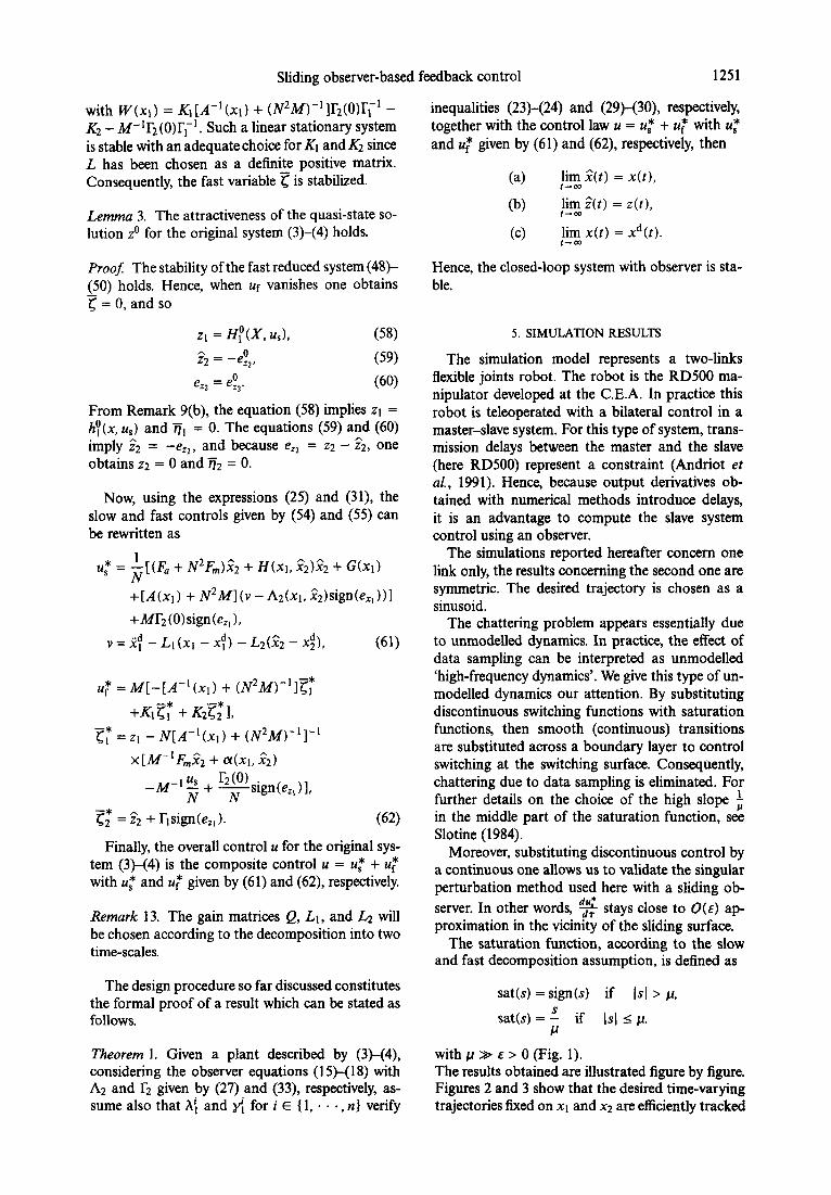
The saturation function, according to the slow and fast decomposition assumption, is defined as

sat(s) = sign(s) if IsI > p,

sat(s) = f if Is1 5 p.

with p >> E > 0 (Fig. 1). The results obtained are illustrated figure by figure. Figures 2 and 3 show that the desired time-varying trajectories fixed on xi and x2 are efficiently tracked

1252 J. Hernandez and J.-P Barbot

Fig. 1. Saturation function.

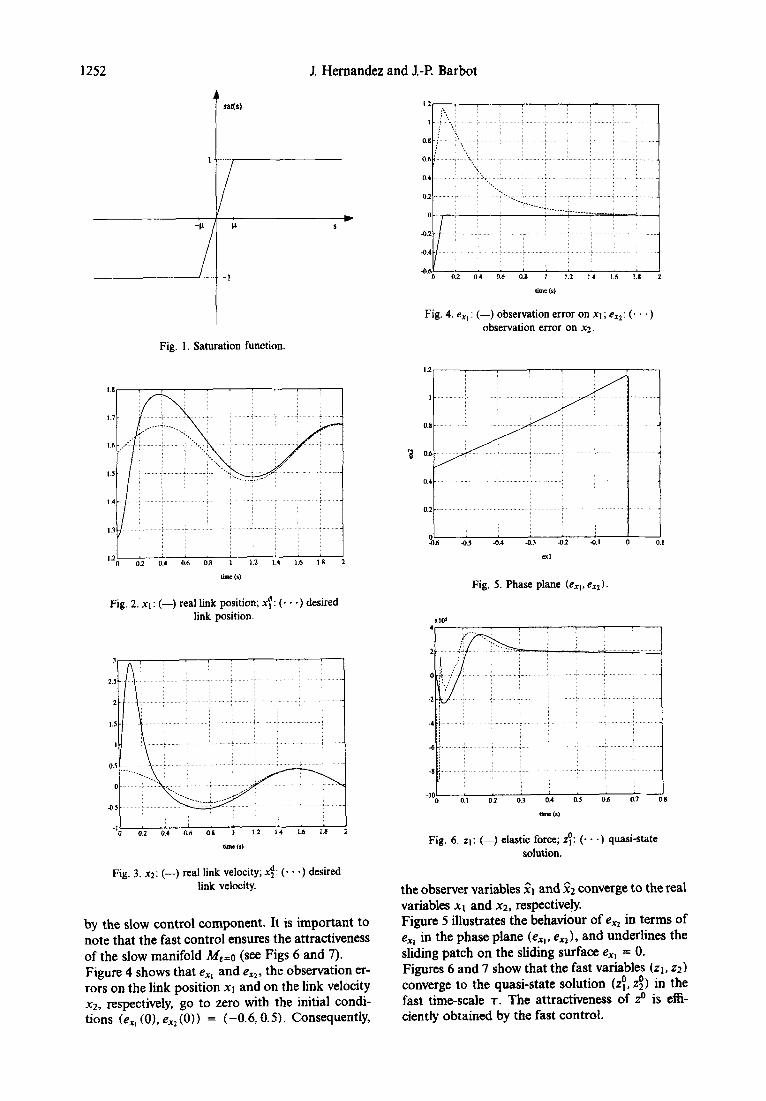
Fig. 2. x1: (-) real link position; x;‘: (, . -) desired link position.

Fig. 3. x2: (-) real link velocity; xi: (. - -) desired link velocity.

by the slow control component. It is important to note that the fast control ensures the attractiveness of the slow manifold ME=0 (see Figs 6 and 7). Figure 4 shows that ex, and exZ, the observation errors on the link position XI and on the link velocity x2, respectively, go to zero with the initial conditions (e,, (O), e,, (0)) = (-0.6,0.5). Consequently,

Fig. 4. e,, : (-) observation error on XI; e,,: (. . 4) observation error on x2.

0.1

Fig. 5. Phase plane (e,,, exz).

Fig. 6. ZI: (-) elastic force; z$ (a . .) quasi-state solution.

the observer variables x^l and $2 converge to the real variables xl and x2, respectively. Figure 5 illustrates the behaviour of exZ in terms of ex, in the phase plane ( ex, , e, 1, and underlines the sliding patch on the sliding surface ex, = 0. Figures 6 and 7 show that the fast variables (ZI, ~2) converge to the quasi-state solution (zi, 2;) in the fast time-scale T. The attractiveness of z” is efficiently obtained by the fast control.


4

xl”’ 2

I-

0.5 -

O-

0 -0.5 -

-I -

.,.s

2.

25 -1 0 I * 3 4 5

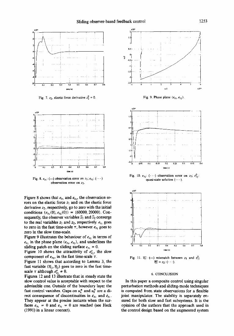
Fig, 7. ~2, elastic force derivative zi = 0. Fig. 9. Phase plane (e;,, eZz).

5

4.

3-

2-

I:

: _..-~~~~--~~-~~---~-~--.-...*.........___~__~__~_ _______

Ojj ::

_I.$

jj

-2-1

-3 0 "., 0.2 0.3 0.4 0.5 "6 0.7 0.8

lime CR)

Fig. 8. e,,: (-) observation error on 21; e,,: (a . *) observation error on 22.

Fig. 10. e,,: (. . a) observation error on 22; ef2: quasi-state solution (= . .).

Figure 8 shows that err and er2, the observation errors on the elastic force zi and on the elastic force derivative 22, respectively, go to zero with the initial conditions (eZ, (01, eZZ (0)) = (60000,20000). Con- sequently, the observer variables $1 and 22 converge to the real variables zi and 22, respectively. er, goes to zero in the fast time-scale T, however er2 goes to zero in the slow time-scale.

2-

Figure 9 illustrates the behaviour of e,, in terms of e,, in the phase plane (e,, , e,,), and underlines the sliding patch on the sliding surface e,, = 0. Figure 10 shows the attractivity of e$, the slow component of e,,, in the fast time-scale T.

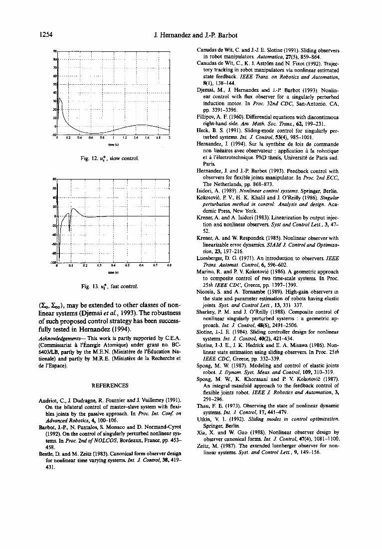
Figure 11 shows that according to Lemma 3, the fast variable (vi, qz) goes to zero in the fast time- scale T although e& + 0. Figures 12 and 13 illustrate that in steady state the slow control value is acceptable with respect to the admissible one. Outside of the boundary layer the fast control vanishes. Gaps on U: and U: are a direct consequence of discontinuities in &, and &,, . They appear at the precise instants when the surfaces eX, = 0 and er, = 0 are reached (see Heck (19911 in a linear context).

Fig. 11. q: (-) mismatch between ZI and .ry; ijT = 22: (. . a).

6. CONCLUSION

In this paper a composite control using singular perturbation methods and sliding-mode techniques is computed from state observations for a flexible joint manipulator. The stability is separately en- sured for both slow and fast subsystems. It is the opinion of the authors that the approach used in the control design based on the aumnented svstem

4

1254 J. Hernandez and J.-F? Barbot

!a, , , , , , , , , ,

Fig. 12. u,*, slow control.

80

Fig. 13. u:, fast control.

(CO, Z,,), may be extended to other classes of nonlinear systems (Djemai et al., 1993). The robustness of such proposed control strategy has been success- fully tested in Hernandez (1994). Acknowledgements- This work is partly supported by C.E.A. (Commissariat a I’Energie Atomique) under grant no. BC- 6403/LB, partly by the M.E.N. (Minis&e de I’Education Na- tionale) and partly by M.R.E. (Ministere de la Recherche et de 1’Espac-e).

REFERENCES

Andriot, C., J. Dudragne, R. Fournier and J. Vuillemey (1991). On the bilateral control of master-slave system with flexi- bles joints by the passive approach. In Proc. Int. ConJ on

Advanced Robotics, 4, 100-106. Barbot, J.-P, N. Pantalos, S. Monaco and D. Normand-Cyrot

(1992). On the control of singularly perturbed nonlinear systems. In Proc. 2nd of NOLCOS, Bordeaux, France, pp. 453- 458.

Bestle, D. and M . Zeitz (1983). Canonical form observer design for nonlinear time varying systems. Znt. J Control, 38,419- 431.

Canudas de Wit, C. and J.-J. E. Slotine (1991). Sliding observers in robot manipulators. Automatica, 27(S), 859-864.

Canudas de Wit, C., K. J. Astrom and N. Fixot (1992). Trajec- tory tracking in robot manipulators via nonlinear estimated state feedback. IEEE Trans. on Robotics and Automation, 8(l), 138-144.

Djemai, M., J. Hernandez and J.-P Barbot (1993). Nonlin- ear control with flux observer for a singularly perturbed induction motor. In Proc. 32nd CDC, San-Antonio, CA, pp. 3391-3396.

Fillipov, A. F. (1960). Differential equations with discontinuous right-hand side. Am. Math. Sot. Trans., 62, 199-23 1.

Heck, B. S. (1991). Sliding-mode control for singularly perturbed systems. Int. I Control, 53(4), 985-1001.

Hernandez, J. (1994). Sur la synthbse de lois de commande non lindaires avec observateur : application a la robotique et a l’electrotechnique. PhD thesis, Universite de Paris sud. Paris.

Hernandez, J. and J.-P Barbot (1993). Feedback control with observers for flexible joints manipulator. In Proc. 2nd ECC, The Netherlands, pp. 868-873.

Isidori, A. (1989). Nonlinear control systems. Springer, Berlin. Kokotovic, I? V, H. K. Khalil and 1. O’Reilly (1986). Singular

perturbation method in control: Analysis and design. Aca- demic Press, New York.

Krener, A. and A. Isidori (1983). Linearization by output injection and nonlinear observers. syst and Control Lett., 3, 47- 52.

Krener, A. and W. Respondek (1985). Nonlinear observer with linearizable error dynamics. SIAM J Controt and Optimiza- tion, 23, 197-216.

Luenberger, D. G. (1971). An introduction to observers. IEEE Trans. Automat. Control, 6, 596-602.

Marino, R. and P V. Kokotovic (1986). A geometric approach to composite control of two time-scale systems. In Proc. 25th IEEE CDC, Greece, pp. 1397-1399.

Nicosia, S. and A. Tornambe (1989). High-gain observers in the state and parameter estimation of robots having elastic joints. Syst. and Control Len., 13, 331-337.

Sharkey, I? M. and J. O’Reilly (1988). Composite control of nonlinear singularly perturbed systems : a geometric approach. Int. .I Control, 48(6), 2491-2506.

Slotine, J.-J. E. (1984). Sliding controller design for nonlinear systems. Int. J. Control, 40(2), 421-434.

Slotine, J.-J. E., J. K. Hedrick and E. A. Misawa (1986). Non- linear state estimation using sliding observers. In Proc. 25th IEEE CDC, Greece, pp. 332-339.

Spong, M. W. (1987). Modeling and control of elastic joints robot. 1 Dynam. Syst. Meas. and Control, 109, 310-319.

Spong, M. W, K. Khorasani and I? V Kokotovic (1987). An integral manifold approach to the feedback control of flexible joints robot. IEEE J Robotics and Automation, 3,

291-296. Thau, F. E. (1973). Observing the state of nonlinear dynamic

systems. ht. J Control, 17,441479. Utkin, V. I. (1992). Sliding modes in control optimization.

Springer, Berlin. Xia, X. and W. Gao (1988). Nonlinear observer design by

observer canonical forms. Int. 1 Control, 47(4), 1081-l 100. Zeitz, M. (1987). The extended luenberger observer for non-

linear systems. Syst. and Control Lett., 9, 149-156.

sliding observer-based feedback control for flexible joints manipulator

Documents