Slides to accompany Weathington, Cunningham & Pittenger (2010),

Chapter 7: Sampling

1

Objectives• Samples, in general• Probability sampling• Probability sampling methods• Nonprobability sampling• Central Limit Theorem• Applications of CLT• Sources of bias and error

2

Why Worry about Sampling?• Don’t worry, just appreciate it

• Objective sampling helps us avoid the Idols of the Cave

– Improving external validity of our conclusions

• “Good” sampling allows us to make comparisons and predictions from our data

3

Samples...• …are (hopefully) valid representatives

of the population you are studying• …can grant you better (more

objective, empirical) data than you will find in anecdotes

• …allow you to avoid reliance on one person’s opinions, perspectives, and biases

4

Probability Examples• Probability of Heads in one flip of a fair coin:

p(H) = 1/2; p(T)=1/2=.5 • p(H and T) in two flips = 2/4=.5 • p(correct answer on 4-option mc question) =

.25• Pr. of choosing a woman in a single random

selection from a class of 223 students with 150 women: p(w)=150/223=.673

5

Probability Sampling• Random: each outcome has an equal

probability of occurring, every time– Every time I flip a coin, the probability is .5

that it will be H or T

• Random sampling depends on this independence of outcomes

• Law of large numbers: On average, a large selection of items will have the same characteristics as those in the population

6

Populations and Samples• Target vs. sampling population

– Target: (universe) e.g. all depressed persons

– Sampling: (accessible) all diagnosed as depressed

• Sampling Frame (all who can be reached)

• Subject (participant pool) – (willing to participate)

• Descriptive data helps us compare our sample against the population

• External validity depends largely on representativeness in sampling

7

Probability Sampling Characteristics• Each population member has an equal

chance of being a potential sample member– No systematic exclusions

• Sampling procedures are based on a protocol– Prevents bias effects on sample selection

• Probability of any specific sample can be calculated– Helps connect results with population

8

Simple Random Sampling• Each population member has equal

probability of selection to the sample

– If selection is random, the sample of any size should represent the population from which it was chosen

• Random numbers are in tables and Excel-type computer programs

9

Simple Random Sampling: How-To• Generate a list of possible participants

(population) in Microsoft Excel• In the next column insert the function

“=RAND()” – Creates a random number between 0 and

1 • Sort both columns by the random numbers• Select the first N individuals for your

sample10

Sequential/Systematic Sampling• Random is not always practical• All sampling population members

are listed and each kth member is selected to the sample

k = sampling interval = Population size

desired sample N

11

Stratified Sampling• Good option when sample needs to

include subgroups from a population– Based on gender, age, education, etc.

• Size of subgroups in final sample must be equivalent to size in population

• Can use simple random or sequential sampling to fill each relative subgroup

12

Cluster Sampling• Good option when participants are already

in groups that cannot be easily separated– e.g., Study of coaching’s impact on

different sports teams• Instead of randomly selecting team

members, you randomly select teams• If need certain subgroup representation,

this may limit your option of teams

13

Nonprobability Sampling• Sampling based on some other factor

besides probability– May be more convenient– May not be as representative

•Can’t establish probabilities associated with sample membership

– Can still be useful if treated with caution

14

Convenience Sampling• “Person” on the street approach

• Sampling from easy to find population members (a “special” subset)

• Sample determined in part by researcher’s sampling method

– Not by probability

• Can bias/distort results

• Sometimes the only option15

Snowball Sampling• Good for cohort studies or when

trying to reach a dispersed population• Using one cohort member to find

others, and so on...• Pros: Good for research on difficult

populations to reach (e.g., homeless)• Cons: No representative sample

guarantee16

Central Limit TheoremRefers to distribution of characteristics

within the probability samples1. As N (sample size) increases, the shape of

the sampling distribution of means will approach a normal distribution

2. µM = µ (mean of sample means =pop mean)

3. σM = σ/√n (SEM)

17

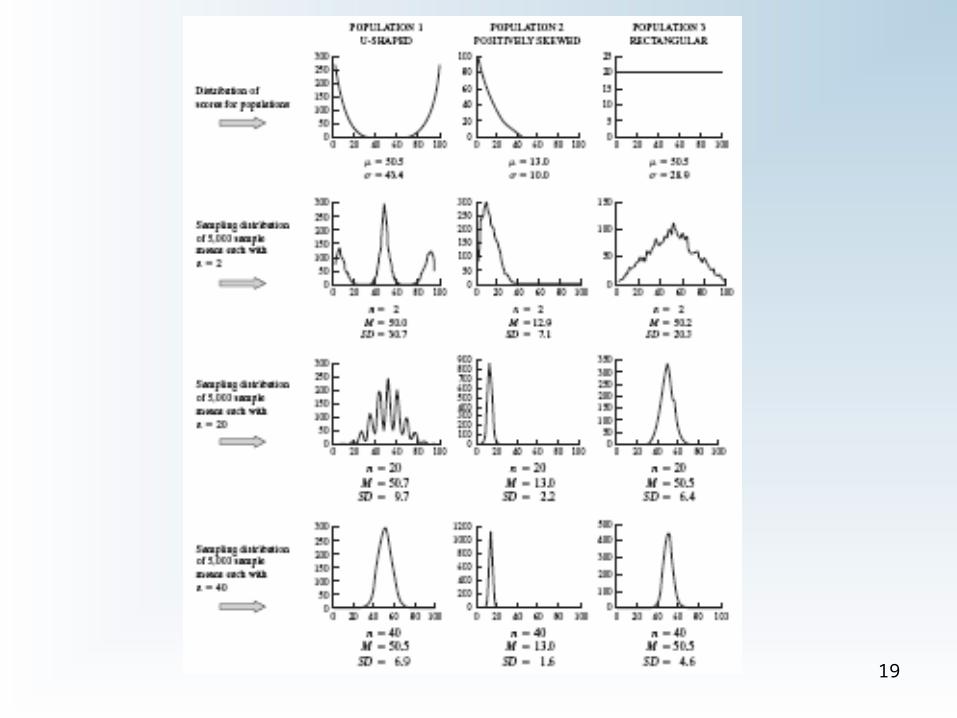
CLT • Sampling Distribution Shape

– Figure 7.4 Note how the M becomes closer to µ as N increases

• µM = mean of means = (sum of all sample means)/(number of samples)

– M = unbiased estimate of µ

• σM = std. dev. of the sampling distribution of M

– As n increases, distribution of sample means will cluster closer to µ more accurate estimate

18

19

CLT• If we use probability sampling, M =

unbiased estimate of µ• M becomes a better estimate of µ

when n increases• We can determine the probability of

obtaining various M

20

Standard Error of the Mean• Represents uncertainty of how well M represents

µ• SEM = SD of sampling distribution of means

σ / √n (n = sample size)

http://www.miniwebtool.com/standard-error-calculator/

• SEM is affected by:– σ as this decreases, SEM decreases–n as this increases, SEM decreases (1/√n)

• M is best estimate of µ when SEM is low21

Applying CLT• Reliability of a sample mean (M)

– Use SEM to calculate confidence intervals around M (see Fig 7.4, p 212)

– There will be variability among sample M, but a CI can help you determine the expected range

• Adequacy of a sample size (n)22

Confidence Intervals• In a normal distribution, 68% of M

within 1 SEM of µ, 95% within 1.96 SEM of, 99% within 2.58 SEM

• Can use CI to predict other M

– 95% CI = 95% of future sample M should fall within this range

23

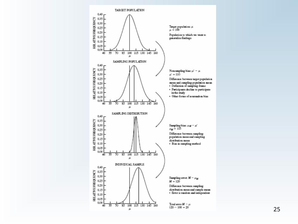
Sources of Bias and Error• Bias: nonrandom, systematic factors that

may make M differ from µ

– Could be controlled

• Error: random events that have the same effect, but cannot be controlled

• Figure 7.7 is a good illustration

– Ideally, µ’ = µ, but not in these examples

– Possible nonsampling biases at work

24

25

Bias and Error• If the sampling is random, then even if

there is a nonsampling bias present, µM

= µ’

• Sampling bias: systematic selection bias while sampling

• Total error = M - µ– Sum of effects from nonsampling bias,

sampling bias, and sampling error26

What is Next?• **instructor to provide details

27