Theoretical Population Biology 75 (2009) 346–354

Contents lists available at ScienceDirect

Theoretical Population Biology

journal homepage: www.elsevier.com/locate/tpb

Site frequency spectra from genomic SNP surveysGaneshkumar Ganapathy a, Marcy K. Uyenoyama b,∗a National Evolutionary Synthesis Center, 2024 W. Main Street, Suite A200, Durham, NC 27705-4667, USAb Department of Biology, Box 90338, Duke University, Durham, NC 27708-0338, USA

a r t i c l e i n f o

Article history:Received 28 December 2008Available online 14 April 2009

Keywords:Site frequency spectrumSingle nucleotide polymorphismEwens’ sampling formulaInfinite-sites modelStandard neutral model

a b s t r a c t

Genomic survey data now permit an unprecedented level of sensitivity in the detection of departuresfrom canonical evolutionary models, including expansions in population size and selective sweeps. Here,we examine the effects of seemingly subtle differences among sampling distributions on goodness offit analyses of site frequency spectra constructed from single nucleotide polymorphisms. Conditioningon the observation of exactly two alleles in a random sample results in a site frequency spectrum thatis independent of the scaled rate of neutral substitution (θ ). Other sampling distributions, includingconditioning on a single mutational event in the sample genealogy or randomly selecting a singlemutation from a genealogywithmultiplemutations, have distinct site frequency spectra that showhighlysignificant departures from the predictions of the biallelic model. Some aspects of data filtering maycontribute to significant departures of site frequency spectra from expectation, apart from any violationof the standard neutral model.

© 2009 Elsevier Inc. All rights reserved.

1. Introduction

1.1. Site frequency spectra

Site frequency spectra (SFSs) are widely used to summarizepatterns of genome-wide variation at the single nucleotidepolymorphisms (SNPs) that abound in virtually all organisms.Fundamental population genetic analyses (Ewens, 1972; Tajima,1989; Fu, 1995; Griffiths and Tavaré, 1998; Stephens, 2000) havecharacterized patterns of genetic variation expected under theinfinite-alleles and infinite-sites models of neutral substitution. Ascaled version of those single-locus predictions now serve as thepoint of departure for the analysis of the SFSs comprising hundredsof thousands of independent SNP loci. Because the relativeexpected multiplicities depend only on sample size, departuresfrom this expectation have been used to identify candidates fortargets of selection or other locus-specific processes (for example,Kim et al. (2007)). Numerical simulation studies (Braverman et al.,1995; Simonsen, 1995) have established that various phenomena,including hitchhiking and expansions in population size, affectspectrum shape, and analytical predictions now exist for a numberof forms of departure from the standard neutral model (Marthet al., 2004; Keightley and Eyre-Walker, 2007; Živkovíc andWiehe,2008).

∗ Corresponding author.E-mail addresses: gg28@duke.edu (G. Ganapathy), marcy@duke.edu

(M.K. Uyenoyama).

0040-5809/$ – see front matter© 2009 Elsevier Inc. All rights reserved.doi:10.1016/j.tpb.2009.04.003

Few spectra constructed from actual genomic SNP surveys con-form to expectation under the standard neutral model. For SNPsidentified by direct sequencing through the NIEHS EnvironmentalGenome Project, for example, Hernandez (2007) noted a generalexcess of derived alleles in low and high multiplicities and a cor-responding deficiency of alleles in intermediate frequencies. As-certainment of SNPs through a small panel of individuals (Nielsenet al., 2004) introduces a different bias, toward an excess of SNPsin intermediate frequencies.

1.2. Fitting to an incorrect model

The sheer volume of information available from genomicdatabases confers unprecedented power to detect departuresfrom models serving as the basis for interpretation of the data.Significant p-values may reflect departures from any aspect ofa model, with some aspects fundamental to key inferences andothers merely incidental.Bishop et al. (1975) have presented a lucid treatment of the

effect on the Pearson chi-square statistic of fitting data to anincorrect model. In a goodness of fit analysis of counts in k cells,the sample X2 corresponds to

X2 =k∑i=1

(ni − npi)2

npi,

for ni the observed count in cell i, n (=∑i ni) the total number

of counts, and pi the expected proportion in cell i. If the trueproportions (p∗i ) of the multinomial distribution from which the

G. Ganapathy, M.K. Uyenoyama / Theoretical Population Biology 75 (2009) 346–354 347

observations (ni) are sampled differ from those used to determinethe expected counts (pi), then the expectation of X2 corresponds to

E[X2] = k− 1+k∑i=1

(p∗i − pi)pi

+ (n− 1)k∑i=1

(p∗i − pi)2

pi(1)

(Bishop et al., 1975, Section 9.6). For the number of counts (n)very large relative to the number of cells (k), as is the case for theanalysis of genomic SNP data, even small departures between thetrue and fitted models ((p∗i − pi)

2≈ ε) can cause the expected X2

to exceed considerably the degrees of freedom (df = k− 1).

1.3. Comparison of sampling distributions

Here, we address the effect on the shape of expected sitefrequency spectra of SNPs of closely related models for theirsampling distribution. Restriction of consideration to samplegenealogies that contain a single mutational event induces adependence of the SFS on the scaled mutation rate (θ = lim 2Nu,for N the effective number of genes and u the rate of neutralsubstitution). This dependence on θ implies that the SFS canprovide a basis for the estimation of this fundamental parameter.Of particular significance for the detection of departures from thestandard neutral model is that we expect classes of SNPs withdistinct rates of neutral substitution to show distinct spectra, evenin the absence of class-specific processes, including selection.We characterize the expected shape of site frequency spectra

constructed from sample genealogies that contain exactly onesegregating site (neutral SNP model). A folded version of themodelwidely used to represent the standard neutralmodel (scaledmultiplicitymodel) follows directly from Ewens’ sampling formula(ESF, Ewens (1972)) conditioned on the observation of exactly twoalleles in the sample.We used ms (Hudson, 2002) to simulate 12 × 106 data sets

from a non-recombining region for a range of values of θ (0.5–6.0).For each data set, we determined the number of segregating sites,the multiplicity of each mutation in the sample, the number ofdistinct haplotypes (alleles), the length of each branch, and thesize of each branch (number of descendent tips). An R file withcode for determiningmaximum likelihood estimates of θ and theirconfidence intervals is provided as Supplementary Data.We conducted a series of goodness of fit analyses to explore

the influence of various means of filtering large data sets toisolate single nucleotide polymorphisms. Our results indicate thatseemingly subtle differences between the theoretical and actualsampling distributions can generate very highly significant X2values in tests involving the large number of observations typical ofgenomic SNP data, quite apart from departures from the standardneutral model.

2. Expected patterns of variation

We summarize basic descriptors of variation.

2.1. Number of segregating sites

On level l of the genealogy of a sample of genes (the segmentcomprising l lineages), the probability of the occurrence of amutation more recently than a coalescence is

lu(l2

)/N + lu

=θ

l− 1+ θ

(see, for example, Ethier and Griffiths (1987)). Watterson (1975)observed that the number of mutations accumulated on levell has a geometric distribution with this parameter, and gavethe probability generating function (pgf) for the total number ofsegregating sites (S) in a sample of size n:

gS(z) =m∏l=2

l− 1l− 1+ θ(1− z)

. (2)

In particular, the expected number of segregating sites corre-sponds to

E[S] = g ′S(1) =m∑l=2

θ

l− 1. (3)

Tavaré (1984) has derived a simple expression for the probabilitymass function of S:

P(S = i|θ) =m− 1θ

m∑l=2

(−1)l−2(m− 2l− 2

)(θ

l− 1+ θ

)i+1. (4)

2.2. Number of mutations with a given multiplicity

For the infinite-sites model, under which all mutations aredetectable and distinguishable, Fu (1995) noted that the numberof genes in a sample that bear a given mutation corresponds tothe number of tips that descend from the branch of the samplegene genealogy on which the mutation arose. Fu (1995) derivedthe mean and variance of the number of mutations in a sample ofsizem that have multiplicity i (ξi):

E[ξi] = θ/i, (5a)

Var[ξi] = θ/i+ σiiθ2, (5b)

in which

σii =

βm(i+ 1) for i < m/2

2(am − ai)/(m− i)− 1/i2 for i = m/2

βm(i)− 1/i2 for i > m/2

with

βm(i) =2m(am+1 − ai)

(m− i+ 1)(m− i)−

2m− i

.

The expected number of mutations present in the sample inmultiplicity i (5a) scaled to the total number of mutations (3),

fs(i|m) =1/i

m−1∑j=11/j, (6)

is widely used to describe the expected SFS for a genomicsample of SNPs, each assumed to correspond to a mutation on anindependent gene genealogy.Expressions closely related or identical to (5) and (6) have been

obtained in a variety of contexts (see especially Watterson (1974)and Griffiths and Tavaré (1998)). In particular, the frequencyof a mutation in the sample provides information about itsage (Kimura andOhta, 1973), and a number of elegant coalescence-based studies have elucidated the genealogical basis of thisrelationship (Griffiths and Tavaré, 1998, 2003; Wiuf and Donnelly,1999; Stephens, 2000; Hobolth and Wiuf, 2009). Tajima (1983,1989) and Griffiths and Tavaré (1998, 2003) showed that (6)corresponds to the expected proportion (rather than number) ofmutations that occur in multiplicity i in a sample of sizem for lowrates of mutation (θ → 0).

348 G. Ganapathy, M.K. Uyenoyama / Theoretical Population Biology 75 (2009) 346–354

2.3. Number of alleles

For the infinite alleles model of mutation, Ewens’ samplingformula provides the joint probability of the numbers in whichdistinct alleles appear in a sample ofm genes:

p(a) =m!

m∏l=1(θ + l− 1)

m∏i=1

(θ

i

)ai 1ai!, (7)

for a = (a1, a2, . . . , am), with ai the number of alleles observedexactly i times. Explicit reference to the genealogy of thesample under the standard neutral model has yielded elegantcombinatorial derivations of the ESF (Kingman, 1978; Donnelly,1986; Griffiths and Lessard, 2005).Ewens (1972) derived the probability mass function for the

number of distinct alleles (K ) observed in a sample of sizem,

P(K = i|θ,m) =liθ i

Lm(θ), (8)

for L(θ) providing the Stirling numbers of the first kind (li):

Lm(θ) = θ(θ + 1) · · · (θ +m− 1)= l1θ + l2θ2 + · · · + lmθm.

This distribution (8) has pgf

gK (z) =Lm(θz)Lm(θ)

=

m∏l=1

θz + l− 1θ + l− 1

.

Ewens (1972) gave the expectation and variance of the number ofalleles:

E[K ] =m∑l=1

θ

θ + l− 1(9a)

Var[K ] =m∑l=1

θ

θ + l− 1−

m∑l=1

(θ

θ + l− 1

)2. (9b)

From the ESF (7), conditioned on the observation of a biallelicsample, we obtain a folded version of the scaledmultiplicitymodel(6), inwhich the ancestral andderived alleles are not distinguished.A random sample ofm genes contains exactly two haplotypes withprobability

P(K = 2) =l2θ2

Lm(θ)= g ′′K (0)/2 =

m∑l=2

θ

l− 1

m∏j=2

j− 1j− 1+ θ

. (10)

Conditioning on this event, we obtain from the ESF (7) theprobability of a sample containing two alleles inmultiplicities i andm− i:

P(ai = 1, am−i = 1|K = 2) =1/i+ 1/(m− i)

m−1∑j=11/j

for i 6= m− i

P(am/2 = 2|K = 2) =2/mm−1∑j=11/j

for i = m− i.

(11)

That θ does not appear in these expressions reflects Ewens’s (1972)finding that the observed number of alleles K provides a sufficientstatistic for the estimation of θ : the joint distribution of allelemultiplicities (7) conditional on K is independent of θ .

Table 1Genetic variation in samples of size 19.

θ Mutation number Biallelic0 1a >1 Countsb %>1 mutc

0.5 204,420 297,831 497,749 357,998 16.81.0 52,737 133,862 813,401 183,449 27.01.5 15,867 54,129 930,004 82,534 34.42.0 5,254 21,975 972,771 36,763 40.22.5 1,866 9,121 989,013 16,555 44.93.0 776 4,190 995,034 8,029 47.83.5 306 1,845 997,849 3,908 52.84.0 128 890 998,982 1,980 55.14.5 66 415 999,519 1,020 59.35.0 29 208 999,763 519 60.05.5 7 99 999,894 273 63.76.0 3 66 999,931 155 57.4a Trees containing a single mutational event.b Samples containing exactly two haplotypes.c % of trees with more than 1 mutation.

2.4. Conditioning on a single segregating site

2.4.1. Neutral SNP modelHere, we use the term SNP to describe a non-recombining locus

atwhich a singlemutational event has occurred in the genealogy ofa sample of genes. We describe sites at which two forms segregatein the sample as biallelic, recognizing SNPs as a subset of this group(see Table 1 for an example).The probability that the genealogy contains a single mutation

and that it lies on level l is

P(SNP, δl = 1) =θ

l− 1+ θ

m∏j=2

j− 1j− 1+ θ

,

for δl an indicator variable that takes the value 1 only if themutation occurs on level l. Summing over levels, we confirm thatthe probability of a SNP is

P(SNP) = g ′S(0) =m∑l=2

θ

l− 1+ θ

m∏j=2

j− 1j− 1+ θ

, (12)

for gS(·) the Watterson pgf (2) of the number of segregatingsites. Comparison of (10) and (12) illustrates the close relationshipbetween conditioning on a single segregating site and conditioningon two segregating alleles: SNPs represent a subset of biallelicpolymorphisms.Conditional on a genealogy containing a single mutation, the

mutation arose on level lwith probability

P(δl = 1|SNP) =1

l−1+θm∑j=2

1j−1+θ

.

Under our neutral SNP model, a SNP-defining mutation occurs inexactly i of them sampled genes with probability

fn(i|m, θ) =

m−i+1∑l=2

1θ+l−1

(m−i−1l−2

)(m−1l−1

)m∑j=2

1θ+j−1

=

1i

m−i+1∑l=2

l−1θ+l−1

(m−li−1

)(m−1i

) m∑j=2

1θ+j−1

, (13)

using Eq. (14) of Fu (1995).

G. Ganapathy, M.K. Uyenoyama / Theoretical Population Biology 75 (2009) 346–354 349

Table 2Derived allele counts in sample genealogies containing a single mutation.

θ 1 2 3 4 5 6 7 8 9 10 11 12 13 14 15 16 17 18

0.5 94,296 45,003 29,118 21,294 16,587 13,523 11,475 9755 8457 7582 6770 6159 5570 5162 4746 4348 4150 38361.0 44,968 21,130 13,334 9,467 7,409 5,908 4,761 4173 3572 3117 2720 2483 2290 1932 1844 1712 1610 14321.5 18,913 8,857 5,487 3,755 2,914 2,326 1,831 1535 1361 1230 1016 958 803 774 671 644 553 5012.0 8,060 3,638 2,180 1,526 1,122 865 727 608 518 442 399 380 343 303 259 227 192 1862.5 3,460 1,509 914 602 484 362 273 243 229 185 160 142 118 110 104 83 76 673.0 1,561 727 424 267 209 179 132 124 104 70 69 58 58 47 57 36 46 223.5 719 310 184 147 91 71 58 43 44 25 28 27 20 20 11 21 19 74.0 327 179 96 49 46 34 29 27 14 15 16 4 12 12 6 10 9 54.5 168 67 45 31 24 13 13 8 6 7 5 6 3 4 5 1 6 35.0 87 38 23 9 8 10 7 3 4 4 6 5 1 1 2 0 0 05.5 36 16 14 9 5 3 3 0 1 1 2 0 2 2 2 2 0 16.0 22 15 9 4 2 2 2 1 1 1 2 2 0 1 1 1 0 0

θ θ

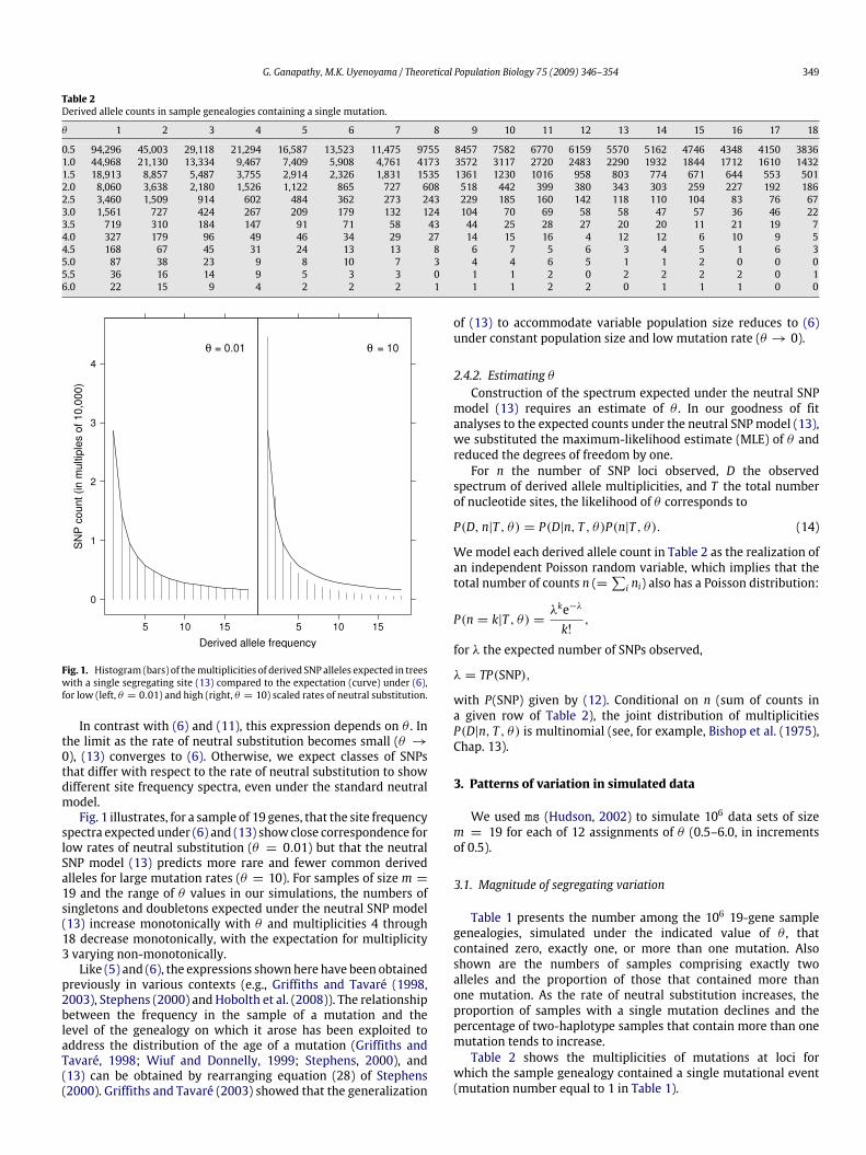
Fig. 1. Histogram (bars) of themultiplicities of derived SNP alleles expected in treeswith a single segregating site (13) compared to the expectation (curve) under (6),for low (left, θ = 0.01) and high (right, θ = 10) scaled rates of neutral substitution.

In contrast with (6) and (11), this expression depends on θ . Inthe limit as the rate of neutral substitution becomes small (θ →0), (13) converges to (6). Otherwise, we expect classes of SNPsthat differ with respect to the rate of neutral substitution to showdifferent site frequency spectra, even under the standard neutralmodel.Fig. 1 illustrates, for a sample of 19 genes, that the site frequency

spectra expected under (6) and (13) show close correspondence forlow rates of neutral substitution (θ = 0.01) but that the neutralSNP model (13) predicts more rare and fewer common derivedalleles for large mutation rates (θ = 10). For samples of size m =19 and the range of θ values in our simulations, the numbers ofsingletons and doubletons expected under the neutral SNP model(13) increase monotonically with θ and multiplicities 4 through18 decrease monotonically, with the expectation for multiplicity3 varying non-monotonically.Like (5) and (6), the expressions shownhere have been obtained

previously in various contexts (e.g., Griffiths and Tavaré (1998,2003), Stephens (2000) and Hobolth et al. (2008)). The relationshipbetween the frequency in the sample of a mutation and thelevel of the genealogy on which it arose has been exploited toaddress the distribution of the age of a mutation (Griffiths andTavaré, 1998; Wiuf and Donnelly, 1999; Stephens, 2000), and(13) can be obtained by rearranging equation (28) of Stephens(2000). Griffiths and Tavaré (2003) showed that the generalization

of (13) to accommodate variable population size reduces to (6)under constant population size and low mutation rate (θ → 0).

2.4.2. Estimating θConstruction of the spectrum expected under the neutral SNP

model (13) requires an estimate of θ . In our goodness of fitanalyses to the expected counts under the neutral SNPmodel (13),we substituted the maximum-likelihood estimate (MLE) of θ andreduced the degrees of freedom by one.For n the number of SNP loci observed, D the observed

spectrum of derived allele multiplicities, and T the total numberof nucleotide sites, the likelihood of θ corresponds to

P(D, n|T , θ) = P(D|n, T , θ)P(n|T , θ). (14)

We model each derived allele count in Table 2 as the realization ofan independent Poisson random variable, which implies that thetotal number of counts n (=

∑i ni) also has a Poisson distribution:

P(n = k|T , θ) =λke−λ

k!,

for λ the expected number of SNPs observed,

λ = TP(SNP),

with P(SNP) given by (12). Conditional on n (sum of counts ina given row of Table 2), the joint distribution of multiplicitiesP(D|n, T , θ) is multinomial (see, for example, Bishop et al. (1975),Chap. 13).

3. Patterns of variation in simulated data

We used ms (Hudson, 2002) to simulate 106 data sets of sizem = 19 for each of 12 assignments of θ (0.5–6.0, in incrementsof 0.5).

3.1. Magnitude of segregating variation

Table 1 presents the number among the 106 19-gene samplegenealogies, simulated under the indicated value of θ , thatcontained zero, exactly one, or more than one mutation. Alsoshown are the numbers of samples comprising exactly twoalleles and the proportion of those that contained more thanone mutation. As the rate of neutral substitution increases, theproportion of samples with a single mutation declines and thepercentage of two-haplotype samples that contain more than onemutation tends to increase.Table 2 shows the multiplicities of mutations at loci for

which the sample genealogy contained a single mutational event(mutation number equal to 1 in Table 1).

350 G. Ganapathy, M.K. Uyenoyama / Theoretical Population Biology 75 (2009) 346–354

Table 3Mean and variance of the number of mutations with the indicated multiplicityunder the infinite-sites model.

Multiplicity Mean VarianceObserveda Expectedb Observeda Expectedc

1 1.0025 1.0000 1.200 1.1992 0.5001 0.5000 0.661 0.6613 0.3332 0.3333 0.471 0.4714 0.2492 0.2500 0.371 0.3725 0.2009 0.2000 0.311 0.3106 0.1664 0.1667 0.267 0.2677 0.1429 0.1429 0.236 0.2368 0.1244 0.1250 0.210 0.2129 0.1102 0.1111 0.190 0.19210 0.1007 0.1000 0.173 0.17111 0.0908 0.0909 0.159 0.15912 0.0833 0.0833 0.148 0.14913 0.0774 0.0769 0.142 0.14014 0.0718 0.0714 0.134 0.13215 0.0658 0.0667 0.123 0.12516 0.0623 0.0625 0.118 0.11917 0.0590 0.0588 0.114 0.11318 0.0556 0.0556 0.108 0.108a Among 106 simulated trees with θ = 1.0.b From (5a).c From (5b).

3.2. Number of mutations having a given multiplicity

Fu’s (1995) analysis addressed the number (rather thanproportion) of mutations that have a given multiplicity in arandom sample genealogy. For each of the 106 sample genealogiessimulated under a given assignment of θ , we distinguished amongall mutations, in accordance with the infinite sites model assumedby Fu (1995), and determined the total number that occurred ineachmultiplicity. Table 3 indicates an excellent fit to the analyticalmean and variance (5) of data simulated under θ = 1.0, and othervalues of θ gave similar results.Fig. 2 shows the number of trees simulated under θ = 6.0

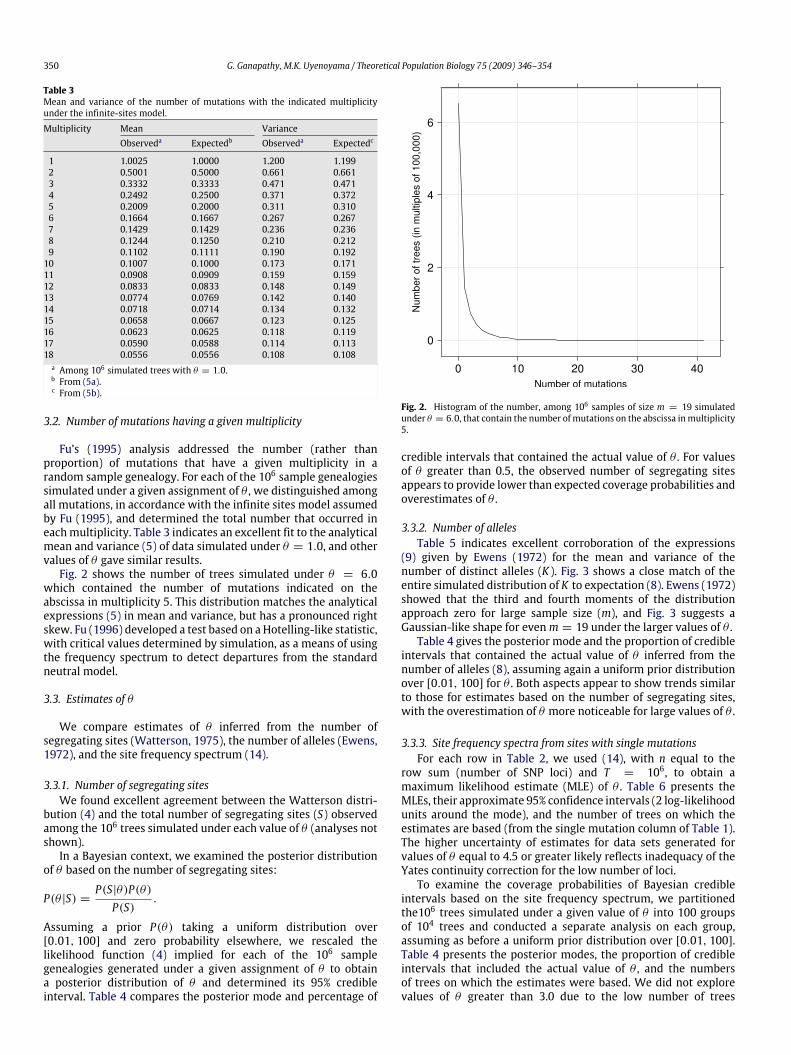
which contained the number of mutations indicated on theabscissa in multiplicity 5. This distribution matches the analyticalexpressions (5) in mean and variance, but has a pronounced rightskew. Fu (1996) developed a test based on aHotelling-like statistic,with critical values determined by simulation, as a means of usingthe frequency spectrum to detect departures from the standardneutral model.

3.3. Estimates of θ

We compare estimates of θ inferred from the number ofsegregating sites (Watterson, 1975), the number of alleles (Ewens,1972), and the site frequency spectrum (14).

3.3.1. Number of segregating sitesWe found excellent agreement between the Watterson distri-

bution (4) and the total number of segregating sites (S) observedamong the 106 trees simulated under each value of θ (analyses notshown).In a Bayesian context, we examined the posterior distribution

of θ based on the number of segregating sites:

P(θ |S) =P(S|θ)P(θ)P(S)

.

Assuming a prior P(θ) taking a uniform distribution over[0.01, 100] and zero probability elsewhere, we rescaled thelikelihood function (4) implied for each of the 106 samplegenealogies generated under a given assignment of θ to obtaina posterior distribution of θ and determined its 95% credibleinterval. Table 4 compares the posterior mode and percentage of

Fig. 2. Histogram of the number, among 106 samples of size m = 19 simulatedunder θ = 6.0, that contain the number ofmutations on the abscissa inmultiplicity5.

credible intervals that contained the actual value of θ . For valuesof θ greater than 0.5, the observed number of segregating sitesappears to provide lower than expected coverage probabilities andoverestimates of θ .

3.3.2. Number of allelesTable 5 indicates excellent corroboration of the expressions

(9) given by Ewens (1972) for the mean and variance of thenumber of distinct alleles (K ). Fig. 3 shows a close match of theentire simulated distribution of K to expectation (8). Ewens (1972)showed that the third and fourth moments of the distributionapproach zero for large sample size (m), and Fig. 3 suggests aGaussian-like shape for evenm = 19 under the larger values of θ .Table 4 gives the posterior mode and the proportion of credible

intervals that contained the actual value of θ inferred from thenumber of alleles (8), assuming again a uniform prior distributionover [0.01, 100] for θ . Both aspects appear to show trends similarto those for estimates based on the number of segregating sites,with the overestimation of θ more noticeable for large values of θ .

3.3.3. Site frequency spectra from sites with single mutationsFor each row in Table 2, we used (14), with n equal to the

row sum (number of SNP loci) and T = 106, to obtain amaximum likelihood estimate (MLE) of θ . Table 6 presents theMLEs, their approximate 95% confidence intervals (2 log-likelihoodunits around the mode), and the number of trees on which theestimates are based (from the single mutation column of Table 1).The higher uncertainty of estimates for data sets generated forvalues of θ equal to 4.5 or greater likely reflects inadequacy of theYates continuity correction for the low number of loci.To examine the coverage probabilities of Bayesian credible

intervals based on the site frequency spectrum, we partitionedthe106 trees simulated under a given value of θ into 100 groupsof 104 trees and conducted a separate analysis on each group,assuming as before a uniform prior distribution over [0.01, 100].Table 4 presents the posterior modes, the proportion of credibleintervals that included the actual value of θ , and the numbersof trees on which the estimates were based. We did not explorevalues of θ greater than 3.0 due to the low number of trees

G. Ganapathy, M.K. Uyenoyama / Theoretical Population Biology 75 (2009) 346–354 351

Table 4Bayesian estimates of θ and coverage probabilities.

Actual θ Segregating sitesa Allele numberb SNP spectrumc

Mode Coveraged Mode Coveraged Mode Coveragee Number of locif

0.5 0.511 95.2 0.559 95.6 0.489 97 2978.31.0 1.027 94.5 1.109 91.3 1.001 99 1338.61.5 1.548 92.9 1.657 88.7 1.501 99 541.32.0 2.075 94.1 2.211 90.7 2.004 93 219.82.5 2.604 93.6 2.769 92.8 2.516 95 91.23.0 3.129 94.3 3.324 94.2 2.990 97 41.93.5 3.664 94.1 3.889 90.84.0 4.196 93.8 4.461 93.14.5 4.730 94.4 5.028 90.65.0 5.259 93.3 5.604 94.75.5 5.796 93.1 6.185 91.46.0 6.332 93.1 6.781 89.2a From (4), based on 106 loci.b From (8), based on 106 loci.c From (13), based on 100 groups of 104 loci.d % of 106 95% credible intervals that contained the true value.e Number out of 100 95% credible intervals that contained the true value.f Average number of loci (of 105 examined) per credible interval.

θ

θ

θ θ

θ

θ

Fig. 3. Histograms (bars) of the observed number of trees that contain the numberof alleles indicated on the abscissa compared to the analytical distribution (curves)from (8).

containing a single segregating site. As for the MLEs in Table 6,the width of the average credible interval increased with θ and thenumber of trees used in the estimation declined. For θ up to 3.0,basing the estimation on the site frequency spectrum appears toimprove accuracy over using only the number of segregating sites(4) or only the number of alleles (8). For higher values of θ , thelow number of trees per group appeared to have compromised theestimation of both the mode and the coverage probability.

4. Goodness of fit of site frequency spectra

4.1. Data restricted to sites with a single mutational event

For the subset of simulated sample genealogies that containeda single segregating site (Table 2), we computed the Pearson chi-square statistic under the scaled multiplicity (6) and neutral SNP(13) models, using the MLEs for θ given in Table 6 for the latter. Toavoid large departures of the counts from approximate continuity

Table 5Observeda and expectedb moments of allele number.

θ Mean VarianceObserved Expected Observed Expected

0.5 2.454 2.454 1.231 1.2331.0 3.549 3.548 1.952 1.9541.5 4.438 4.439 2.447 2.4482.0 5.196 5.195 2.807 2.8112.5 5.857 5.854 3.081 3.0863.0 6.433 6.436 3.301 3.3003.5 6.957 6.958 3.469 3.4684.0 7.431 7.430 3.608 3.6004.5 7.858 7.860 3.705 3.7045.0 8.252 8.255 3.789 3.7855.5 8.617 8.619 3.848 3.8496.0 8.959 8.956 3.900 3.897a Among 106 simulated trees.b From (9).

Table 6Maximum likelihood estimate of θ and approximate confidence interval.

Actual θ MLEa 95% CIb Tree numberc

0.5 0.499 (0.496, 0.502) 297,8311.0 1.001 (0.998, 1.004) 133,8621.5 1.500 (1.495, 1.505) 54,1292.0 2.003 (1.995, 2.010) 21,9752.5 2.513 (2.500, 2.525) 9,1213.0 2.984 (2.965, 3.003) 4,1903.5 3.506 (3.476, 3.537) 1,8454.0 3.991 (3.946, 4.037) 8904.5 4.523 (4.455, 4.595) 4155.0 5.027 (4.927, 5.133) 2085.5 5.591 (5.440, 5.753) 99a Based on (14).b Spanning 2 log likelihood units.c Sample trees with a single segregating site.

(see Section 3.3.3), we excluded from consideration data setsgenerated for values of θ greater than 4.0, for which the expectedcounts in cells representing the highest multiplicities fell below 5.Fig. 4 indicates highly significant departures from the scaled

multiplicity model (6). As expected for a fit to an incorrect model(1), the X2 values tend to increase with number (n) of locicontributing to the SFS. In contrast, Fig. 5, showing the fit tothe correct model (single mutational event), indicates no obviousrelationship between the total number of counts and the X2 valuesobtained under the neutral SNP model (13). While the low X2values for most of the range under θ = 2.5 and high X2 valuesunder θ = 3.5 in Fig. 5 appear unusual, the simulated SNP data

352 G. Ganapathy, M.K. Uyenoyama / Theoretical Population Biology 75 (2009) 346–354

θ θ θ θ

θθθθ

Fig. 4. Sample Pearson chi-square values for the fit to the scaled multiplicitymodel (6) of SFSs generated from simulated SNP data (single mutational event)for samples of m = 19 genes. Shown on the abscissa are the numbers of sets of10,000 loci in the group contributing to the spectrum, with 100 corresponding toall 106 simulated genealogies. The solid line indicates the average X2 value and thedashed line corresponds to the expectation for a fit to the correct model (df = 17,for multiplicities of the derived allele of 1 through 18).

appear to lend much greater support to the correct neutral SNPmodel (13) than to the scaled multiplicity model (6).Fig. 6 shows the empirical cumulative distribution of p-values

from goodness of fit tests to the neutral SNP model (13) for θup to 2.0. For each value of θ , we partitioned the 106 simulatedtrees into 100 groups of 104 simulated trees. Elimination of non-SNP sites (trees showing a number of mutations different from1) reduced the number of loci to the values indicated in therightmost column of Table 4. For each partition, we determinedthe p-value associated with the spectrum constructed from thosesingle-mutation trees. A perfect sample would show equalitybetween the cumulative distribution of p-values and the nominalsignificance level (diagonal line). Fig. 6 suggests a tendency towardfalse positives (Type I error) for θ = 0.5.

4.2. Data restricted to biallelic sites

As noted in Section 2.3, the ESF (7) links the allele frequencyspectrum to the expected number of mutations that occur in asample in a given multiplicity (5a): the ESF, conditioned on theobservation of exactly two alleles in the sample (11), correspondsto the folded version of the scaled multiplicity model (6).Fig. 7 shows for assignments of θ up to 2.5, the X2 values

obtained in goodness of fit tests to the folded scaled multiplicitymodel (11) as a function of the number of sample genealogiesconsidered (n). We refrained from analyzing data simulated forassignments for larger values of θ , for which the expected numberof counts in at least one cell fell below 5. These plots suggestno obvious increase in the X2 values with total count numberas would be expected under fitting to an incorrect model (1). Ofpossible concern in a number of cases is an unusually low X2 value,indicating too good a fit.Application of goodness of fit tests to the neutral SNP model

(13), incorrectly regarding the two alleles segregating in eachsample as defined by a single mutational event, underestimates

θ θ θ θ

θθθθ

Fig. 5. Sample Pearson chi-square values for the fit to the neutral SNP model (13)of SFSs generated from simulated SNP data (single mutational event) for samples ofm = 19 genes. The dashed horizontal line indicates the expectation (df = 16, afterestimation of θ ), with other features as described for Fig. 4.

θ θ θ θ

Fig. 6. Empirical cumulative distribution of p-values obtained for 100 sitefrequency spectra for the neutral SNP model (13) applied to SNP data (singlesegregating site) simulated under the four indicated values of θ . The diagonal linerepresents the nominal significance level.

Table 7Biallelic data fit to the neutral SNP model.

Actual θ MLEa X2 of fitb

0.5 0.272 634.71.0 0.817 2098.81.5 1.265 1809.52.0 1.711 1159.62.5 2.161 725.83.0 2.585 433.03.5 3.024 251.84.0 3.456 171.84.5 3.895 82.55.0 4.361 54.85.5 4.821 51.86.0 5.243 22.8a From (14).b To (13) with df = 16.

θ and generates highly significant X2 values (Table 7). As Fig. 1would suggest, the neutral SNP model predicts too many samplescontaining a rare allele and a corresponding deficiency of sampleswith the two alleles in comparable frequencies. Although theexpectations under the neutral SNP model (13) converge to thoseunder the scaledmultiplicitymodel (6) as θ becomes small, Table 1indicates that even for θ = 0.5, a substantial fraction (nearly 17%)of the simulated biallelic data sets contained more than a singlemutation.

G. Ganapathy, M.K. Uyenoyama / Theoretical Population Biology 75 (2009) 346–354 353

θ θ θ θ θ

Fig. 7. Sample Pearson chi-square values for the fit to the folded scaledmultiplicitymodel (11) of biallelic frequency spectra generated under the indicated θ value.The solid horizontal line represents the average X2 value and the dashed line theexpectation (df = 8).

4.3. Other data sets showing a poor fit to the scaledmultiplicity model

We also explored the effects of other kinds of data filtering,including construction of the spectrum of all mutations (nofiltering) and restriction of consideration to a single randommutation in each tree or to a single random branch in each tree.These data partitions all showed a significantly poor fit to thescaled multiplicity model (6).

4.3.1. Random mutationFor each simulated sample genealogy that contained at least

one mutation, we determined the multiplicity in the sample ofa mutation chosen uniformly at random, without weighting byfrequency in the sample. This subset contains all trees in Table 1except those with zero segregating sites. We found increasingsample X2 values with the number of trees, as in Fig. 4, and amarked departure between the nominal significance level and thecumulative distribution of p-values. Both aspects indicate a verypoor fit to the scaled multiplicity model (6).

4.3.2. Size of a random branchFor a given simulated genealogy, we sampled a branch at

random,weighting by length relative to the total length of the tree,and determined the number of tips descendent from that branch.While the number of descendants is not generally observable, thisexperiment permits us to examine branch size apart from theadditional stochastic process of mutation. As the scaled neutralsubstitution rate θ does not affect the size of a branch, our msoutput provides a total of 12 × 106 simulated samples suitablefor this analysis. A very highly significant departure of simulatedspectra from the spectrum expected under the scaled multiplicitymodel (6) is evident even from subsets of the data. For example,Table 8 compares the observed branch sizes and the expectationsunder the scaled multiplicity model (6) for a subsample of 106trees. Relative to predictions from the scaled multiplicity model(6), the observed trees showed an excess of branches of size 1through 4 and a deficiency of branches of all larger sizes. A fit to thescaledmultiplicitymodelwould indicate a particularly large excess(18,371) of singletons (terminal branches 1), with this multiplicityclass contributing almost 35% of the total X2 value (3412, withdf = 17), even in the absence of population expansions or selectivesweeps.

4.3.3. All segregating sitesAlthough the relative numbers of alleles ormutations in a given

sample genealogy are of course correlated (7), we constructedthe spectrum of all mutations observed in many sample treesgenerated under a given value of θ , expecting correlations betweenmutations on the same tree to be dwarfed by the large numberof independent trees. We partitioned the 106 samples simulatedunder each value of θ into 100 groups of 104 trees and determinedthe p-value associated with a fit to the scaled multiplicity model(6). The empirical cumulative distribution of p-values for the 1200tests using all 12 × 106 simulated trees indicated a very poor fit,with 80% of the tests giving p-values less than 0.04.

Table 8Observed and expected branch size distributions.

Branch sizea Observedb Expectedc ∆d

1 304,485 286,114 18,3712 148,412 143,057 53553 96,429 95,371 10584 71,645 71,529 1165 56,205 57,223 −10186 46,430 47,686 −12567 39,769 40,873 −11048 33,833 35,764 −19319 29,937 31,790 −185310 26,607 28,611 −200411 23,834 26,010 −217612 22,045 23,843 −179813 20,317 22,009 −169214 18,495 20,437 −194215 17,004 19,074 −207016 15,778 17,882 −210417 15,005 16,830 −182518 13,770 15,895 −2125a Number of descendant tips of a random branch.b Among 106 simulated trees.c From the scaled multiplicity model (6).d 1 = Observed−Expected.

5. Discussion

5.1. Dependence of SNP site frequency spectra on θ

Fundamental to the interpretation of site frequency spectraconstructed from surveys of genomic variation are the analysesof Ewens (1972) and Fu (1995) for the infinite-alleles and infinite-sites model of mutation, respectively. We note that the foldedversion of the scaled multiplicity model (6) can be obtaineddirectly from the ESF (7), conditioned on biallelic samples (11).A striking property of the ESF (7) is that the allele frequencyspectrum conditioned on the number of observed alleles (K ) isindependent of θ (Ewens, 1972). This property is shared by thescaledmultiplicitymodel (6), which iswidely used to represent theexpected SFS under the standard neutral model for genome-wideSNP data.In contrast, the observed SFS for sample genealogies that

contain a single mutational event (13) does in fact provideinformation about θ , implying that site frequency spectra canprovide a basis for the estimation of this fundamental parameter.Tables 4 and 6 indicate high accuracy of both Bayesian andmaximum likelihood estimates of θ for data sets comprising 103or more SNPs. Liu et al. (in press) have recently developed ageneralized least squares method for estimating θ using Fu’s(1995) expressions for themeans and covariances (5) of the counts(rather than proportions) of mutations across multiplicities.Our analysis suggests that differences between the sampling

distributions imposed by restriction to biallelic variation (11)and by restriction to single mutational events (13) are readilydetectable in analyses incorporating the volume of data typicalof genomic SNP surveys. SNPs constitute a subset of biallelicpolymorphisms, and theprobability of a single segregating site (12)is nearly identical to the probability of a biallelic polymorphism(10). However, our simulated data (Table 1) illustrate that forlarge θ a substantial proportion of biallelic polymorphisms maycomprise multiple segregating mutations in the genealogy ofthe sample. Incorrect application of the neutral SNP model (13),which assumes a single segregating site, results in substantialunderestimation of θ and highly significant X2 values in goodnessof fit analyses (Table 7). Similarly, data restricted to samplegenealogies containing a single segregating site show highlysignificant departures (Fig. 4) from the scaled multiplicity model(6) or the biallelic model (11), while giving strong support to thecorrect neutral SNP model (Figs. 5 and 6).

354 G. Ganapathy, M.K. Uyenoyama / Theoretical Population Biology 75 (2009) 346–354

As has been shown in various contexts (Griffiths and Tavaré,1998, 2003; Stephens, 2000), the neutral SNP model (13) reducesto the scaled multiplicity model (6) in the limit of low ratesof neutral substitution (θ → 0). As θ increases, samplesconditioned on a single segregating site showmore raremutationsand fewer common mutations (Fig. 1). Because an excess of rarevariants is an iconic signature of selective sweeps or expansions ineffective population size (Braverman et al., 1995; Simonsen, 1995),our results suggest that careful consideration of the samplingdistribution of genomic variation may help to avoid unwarrantedinferences about the operation of locus-specific evolutionaryprocesses.

5.2. Departures from the scaled multiplicity model

We found that sampling distributions that show only subtlenumerical and conceptual departures from canonical models canbe very strongly rejected on the basis of sufficiently large numbersof observations. Describing kinds of neutral variation that showpoor fits to the scaled multiplicity model (6) may be as valuableas confirming the fit to expectation of data generated under thecorrect model.Single nucleotide polymorphisms may be considered similar

to polymorphisms due to a single mutational event in a samplegenealogy, regardless of the total number of events in the tree.However, we observed very highly significant deviations from thescaled multiplicity model (6) of site frequency spectra generatedby extracting a single random mutation from simulated trees.Similarly, the distributions of the size (number of descendenttips) of a randomly chosen branch and the multiplicities ofall segregating sites do not fit the scaled multiplicity model(Section 4.3).

5.3. Modelling actual SNP data

We found that the allele frequency spectra generated byrestricting simulated data to biallelic samples fit the folded scaledmultiplicitymodel (11) verywell (Fig. 7) and theneutral SNPmodel(13) very poorly (Table 7). Conversely, simulated data restricted tosample genealogies that contained a single mutational event gavestrong support to the neutral SNP model and strongly rejected thescaled multiplicity model (Section 4.1).We suggest that neither model describes actual SNP data.

Segregation of exactly two nucleotide bases in a sample mayreflect multiple independent substitutions of the same derivedbase for the ancestral base or back mutations, in violation of boththe infinite-sites (5) and infinite-alleles models (7) as well as theneutral SNP model (13). Of the standard models of mutation ofpopulation genetics, SNPs may conform most closely to a finite-sites, K -allele model, in which new mutations assume one offour states (A, C, G, or T). The question as to whether actual SNPsshow site frequency spectra similar to those expected for thestandard neutralmodel under thismutation process awaits furtheranalytical and statistical development.

Acknowledgments

In a lifetime of work, Sam Karlin transformed several entirefields. It continues to be an honor to learn from him, to drawupon the part of his work that extended into evolutionarybiology, and to contribute to this memorial volume. We aregrateful to the anonymous reviewers for valuable comments and

references to key works, Asger Hobolth for important insights, andBenjamin D. Redelings for questioning the interpretation of SNPspectra. Support from the National Evolutionary Synthesis Center(NESCent), Durham, NC, for a NESCent Postdoctoral Fellowship toGG and for the Genomic Introgression working group is gratefullyacknowledged. Public Health Service grant GM 37841 (MKU)provided partial support for this research.

References

Bishop, Y.M.M., Fienberg, S.E., Holland, P.W., 1975. Discrete Multivariate Analysis:Theory and Practice. The MIT Press.

Braverman, J.M., Hudson, R.R., Kaplan, N.L., Langley, C.H., Stephan, W., 1995. Thehitchhiking effect on the site frequency spectrum of DNA polymorphism.Genetics 140, 783–796.

Donnelly, P., 1986. Partition structures, Polya urns, the Ewens sampling formula,and the ages of alleles. Theor. Popul. Biol. 30, 271–288.

Ethier, S.N., Griffiths, R.C., 1987. The infinitely-many-sites model as a measure-valued diffusion. Ann. Probab. 15, 515–545.

Ewens, W.J., 1972. The sampling theory of selectively neutral alleles. Theor. Popul.Biol. 3, 87–112.

Fu, Y.-X., 1995. Statistical properties of segregating sites. Theor. Popul. Biol. 48,172–197.

Fu, Y.-X., 1996.Newstatistical tests of neutrality forDNA samples fromapopulation.Genetics 143, 557–570.

Griffiths, R.C., Lessard, S., 2005. Ewens’ sampling formula and related formulae:combinatorial proofs, extensions to variable population size and applicationsto ages of alleles. Theor. Popul. Biol. 68, 167–177.

Griffiths, R.C., Tavaré, S., 1998. The age of a mutation in a general coalescent tree.Commun. Statist. Stoch. Models 14, 273–295.

Griffiths, R.C., Tavaré, S., 2003. The genealogy of a neutral mutation. In: Green, P.J.,Hjort, N.L., Richardson, S. (Eds.), Highly Structured Stochastic Systems. OxfordUniv. Press, Oxford, pp. 393–412 (Chapter 13).

Hernandez, R.D., Williamson, S., Bustamante, C.D., 2007. Context dependence,ancestral misidentification, and spurious signatures of natural selection. Mol.Biol. Evol. 24, 1792–1800.

Hobolth, A., Uyenoyama, M.K., Wiuf, C., 2008. Importance sampling for the infinitesites model. Statist. Appl. Genetics Mol. Biol. 7, Article 32.

Hobolth, A., Wiuf, C., 2009. The genealogy, site frequency spectrum and ages of twonested mutant alleles. Theor. Popul. Biol. 75 (4), 260–265.

Hudson, R.R., 2002. Generating samples under a Wright-Fisher neutral model ofgenetic variation. Bioinformatics 18, 337–338.

Keightley, P.D., Eyre-Walker, A., 2007. Joint inference of the distribution offitness effects of deleterious mutations and population demography based onnucleotide polymorphism frequencies. Genetics 177, 2251–2261.

Kim, S., Plagnol, V., Hu, T.T., Toomajian, C., Clark, R.M., Ossowski, S., Ecker, J.R.,Weigel, D., Nordborg, M., 2007. Recombination and linkage disequilibrium inArabidopsis thaliana. Nat. Genet. 39, 1151–1155.

Kimura, M., Ohta, T., 1973. The age of a neutral mutant persisting in a finitepopulation. Genetics 75, 199–212.

Kingman, J.F.C., 1978. Random partitions in population genetics. Proc. Roy. Soc.London A 361, 1–20.

Liu, X., Maxwell, T.J., Boerwinkle, E., Fu, Y.-X., 2009. Inferring population mutationrate and sequencing error rate using the SNP frequency spectrum in a sampleof DNA sequences. Mol. Biol. Evol., in press (doi:10.1093/molbev/msp059).

Marth, G.T., Czabarka, E., Murvai, J., Sherry, S.T., 2004. The allele frequencyspectrum in genome-wide human variation data reveals signals of differentialdemographic history in three large world populations. Genetics 166, 351–372.

Nielsen, R., Hubisz, M.J., Clark, A.G., 2004. Reconstituting the frequency spectrum ofascertained single-nucleotide polymorphism data. Genetics 168, 2372–2382.

Simonsen, K.L., Churchill, G.A., Aquadro, C.F., 1995. Properties of statistical tests ofneutrality for DNA polymorphism data. Genetics 141, 413–429.

Stephens, M., 2000. Times on trees, and the age of an allele. Theor. Popul. Biol. 57,109–119.

Tajima, F., 1989. Statistical method for testing the neutral mutation hypothesis byDNA polymorphism. Genetics 123, 585–595.

Tajima, F., 1983. Evolutionary relationship of DNA sequences in finite populations.Genetics 105, 437–460.

Tavaré, S., 1984. Line-of-descent and genealogical processes, and their applicationsin population genetics models. Theor. Popul. Biol. 26, 119–164.

Watterson, G.A., 1975. On the number of segregating sites in genetical modelswithout recombination. Theor. Popul. Biol. 7, 256–276.

Watterson, G.A., 1974. The sampling theory of selectively neutral alleles. Adv. Appl.Probab. 6, 463–488.

Wiuf, C., Donnelly, P., 1999. Conditional genealogies and the age of a neutralmutant.Theor. Popul. Biol. 56, 183–201.

Živkovíc, D., Wiehe, T., 2008. Second-order moments of segregating sites undervariable population size. Genetics 180, 341–357.