simultaneous computation of dynamical and …cstringer/papers/we.pdfsimultaneous computation of...

Simultaneous Computation of Dynamical and EquilibriumInformation Using a Weighted Ensemble of TrajectoriesErnesto Suarez,†,∥ Steven Lettieri,†,∥ Matthew C. Zwier,‡ Carsen A. Stringer,§

Sundar Raman Subramanian,† Lillian T. Chong,‡ and Daniel M. Zuckerman*,†

†Department of Computational and Systems Biology, University of Pittsburgh, 4200 Fifth Ave, Pittsburgh, Pennsylvania 15260,United States‡Department of Chemistry, University of Pittsburgh, 4200 Fifth Ave, Pittsburgh, Pennsylvania 15260, United States§Gatsby Computational Neuroscience Unit, University College London, Gower St, London WC1E 6BT, United Kingdom

*S Supporting Information

ABSTRACT: Equilibrium formally can be represented as an ensemble of uncoupledsystems undergoing unbiased dynamics in which detailed balance is maintained. Manynonequilibrium processes can be described by suitable subsets of the equilibrium ensemble.Here, we employ the “weighted ensemble” (WE) simulation protocol [Huber and Kim,Biophys. J. 1996, 70, 97−110] to generate equilibrium trajectory ensembles and extractnonequilibrium subsets for computing kinetic quantities. States do not need to be chosenin advance. The procedure formally allows estimation of kinetic rates between arbitrarystates chosen after the simulation, along with their equilibrium populations. We alsodescribe a related history-dependent matrix procedure for estimating equilibrium andnonequilibrium observables when phase space has been divided into arbitrary non-Markovian regions, whether in WE or ordinary simulation. In this proof-of-principle study, these methods are successfully appliedand validated on two molecular systems: explicitly solvated methane association and the implicitly solvated Ala4 peptide. Wecomment on challenges remaining in WE calculations.

1. INTRODUCTION

Although it is textbook knowledge that the functions ofbiomacromolecules are strongly coupled to their conforma-tional motions and fluctuations,1 computer simulation of suchmotions has been a challenge for decades.2 Typically, distinctalgorithms are employed to estimate equilibrium quantities(e.g., refs 3 and 4) and dynamical properties (e.g., refs 5−10).In principle, a single long dynamics trajectory would besufficient to determine both equilibrium and dynamicalproperties,11 but such simulations remain impractical for mostsystems of interest.Aside from straightforward simulations, more technical

approaches that can yield both equilibrium and dynamicalsimulation, sometimes under minor assumptions, have drawnincreasing attention. A number of approaches employ Markovstate models (MSMs) as part their overall computationalstrategy. On the basis of replica exchange molecular dynamics(REMD),12,13 it is possible to extract kinetic information fromcontinuous trajectory segments between exchanges and therebyconstruct an MSM.13 The adaptive seeding method (ASM)similarly builds an MSM based on trajectories seeded fromstates discovered via REMD or another of the so-calledgeneralized ensemble (GE) algorithms.14 MSMs have also beenused in combination with short, off-equilibrium simulations toconstruct the equilibrium ensemble of folding pathways of aprotein.15

Another general strategy is to employ a series of non-intersecting interfaces that interpolate between states of interestselected in advance. Milestoning generates and analyzestransitions between interfaces assuming prior history does notaffect the distribution of trajectories.16,17 Transition interfacesampling (TIS)18,19 and its variants also analyze suchtransitions and can yield free energy barriers in addition torates while accounting for some history information.20 Forwardflux sampling (FFS) again samples interface transitions: itaccounts for history information and can yield rates andequilibrium information.7,21

The “weighted ensemble” (WE) simulation strategy5 (seeFigure 1), which has a rigorous basis as a path-samplingmethod,22 has also been suggested as an approach forcomputation of both equilibrium and nonequilibrium proper-ties.23,24 Although WE was originally developed as a tool forcharacterizing nonequilibrium dynamical pathways and rates(e.g., refs 5, 25−28), the strategy was extended to steady-stateconditions including equilibrium.23 The simultaneous compu-tation of equilibrium and kinetic properties using WE wasdemonstrated with configuration space separated into twostates by a dividing surface24 and later for arbitrary states

Special Issue: Free Energy Calculations: Three Decades of Adventurein Chemistry and Biophysics

Received: December 9, 2013Published: March 3, 2014

Article

pubs.acs.org/JCTC

© 2014 American Chemical Society 2658 dx.doi.org/10.1021/ct401065r | J. Chem. Theory Comput. 2014, 10, 2658−2667

Open Access on 03/03/2015

pubs.acs.org/JCTC

http://pubs.acs.org/page/policy/authorchoice/index.html

defined in advance of a simulation.29 In contrast to many otheradvanced sampling strategies, WE generates an ensemble ofcontinuous trajectories, all at the physical condition (e.g.,temperature) of interest.Here, we further develop the capability of WE simulation to

calculate equilibrium and nonequilibrium quantities simulta-neously in several ways that may be important for future studiesof increasingly complex systems. (i) The approach describedbelow permits the calculation of rates between arbitrary states,which can be defined af ter a simulation has been completed. Ina complex system, the most important physical states, includingintermediates, generally will not be obvious prior to simulation.Further, the present approach opens up the possibility to userate calculations to aid in the state-definition process. (ii) Thenon-Markovian analysis described here enables unbiased ratecalculations in the typical case where “bins” used by WEsimulation do not exhibit Markovian behavior. The analysis isgeneral and can be applied outside the WE context, includingthe analysis of ordinary long trajectories. (iii) The non-Markovian analysis can improve the efficiency of WEsimulations by yielding accurate estimates of observables fromshorter simulations. The analysis is based on a previouslysuggested decomposition of the equilibrium ensemble into twononequilibrium steady states.9,20,21,30,31

Generally speaking, WE provides an attractive basis forcomplex simulations. WE is easily parallelizable because itemploys multiple trajectories and was recently used with 3500cores.32 Because there is no need to “catch” trajectories atprecise transition interfaces, WE algorithms lend themselves toa scripting-like implementation which has been employed tostudy a wide range of stochastic systems via regular moleculardynamics,28 Monte Carlo,26 the string strategy,33 and Gillespie-algorithm dynamics of chemical kinetic networks.34

2. THEORETICAL FORMULATIONWE simulation uses multiple simultaneous trajectories, withweights that sum to one, that are occasionally coupled byreplication or combination events every τ units of time.5 Thecoupling events typically are governed by a static partition ofconfiguration space into “bins” (Figure 1c), althoughdynamical/adaptive bins may be used.22 In the case of staticbins, when one or more trajectories enters an unoccupied bin,those trajectories are replicated so that their count conforms toa (typically) preset value, M. Replicated “daughter” trajectoriesinherit equal shares of the parent’s weight. If more than Mtrajectories are found to occupy a bin, trajectories are combinedstatistically in a pairwise fashion until M remain, with weightfrom pruned trajectories assigned to others in the same bin.

These procedures are carried out in such a way that dynamicsremain statistically unbiased.22 This study does not adjustweights according to previously developed reweightingprocedures23 during the simulation. Rather, the WE simulationsdescribed here are long enough to permit relaxation to theequilibrium state.

2.1. Direct Calculation of Observables. Once theequilibrium state is reached in a WE simulation, meaning thatthere is a detailed balance of probability flow between any twostates, equilibrium observables such as state populations or apotential of mean force can be calculated simply by summingtrajectory weights in the corresponding regions of phase space.We term this “direct” estimation of observables.To calculate rates, the equilibrium set of trajectories (Figure

1a) is decomposed into two steady states as shown in Figure1b: the α steady state consisting of trajectories more recently inA than B, and the β steady state with those most recently inB;9,31 these were denoted “AB” and “BA” steady states,respectively, in ref 31. Trajectories are “labeled” according tothe last state visited, i.e., classified as α or β, during a WEsimulation or in a postsimulation analysis (“post-analysis”). Thedirect rate kAB estimate is computed from the probabilityarriving at the final state4,7,9,20,23,35 via

αα

=→

= → |k

p1

MFPT(A B)Flux(A B )

( )AB(1)

where MFPT is the mean-first-passage time, Flux(A → B|α) isthe probability per unit time arriving at state B in the α steadystate, and p(α) is the total probability in the α steady state. Byconstruction p(α) + p(β) = 1. Normalizing by p(α) effectivelyexcludes the reverse steady state, and the rate calculation only“sees” the unidirectional α steady state as in ref 23. Anexpression analogous to eq 1 applies for kBA. Also note that theeffective first order rate constant, defined by Flux(A → B|α)/pAeq, can be determined from equilibrium WE simulationbecause PA

eq can be directly computed by summing weights in A.We note that analogous direct calculation of observables can

be performed from an equilibrium ensemble of unweighted(i.e., “brute force”) trajectories by assigning equal weights toeach.

2.2. Non-Markovian Matrix Calculation of Observ-ables. Beyond the direct estimates of observables based ontrajectory weights, we also generalize previous matrixformulations for nonequilibrium steady states9,30,36 into anequilibrium formulation that explicitly accounts for theembedded steady states (as in Figure 1b,c). These non-Markovian matrix estimates are tested below and may prove

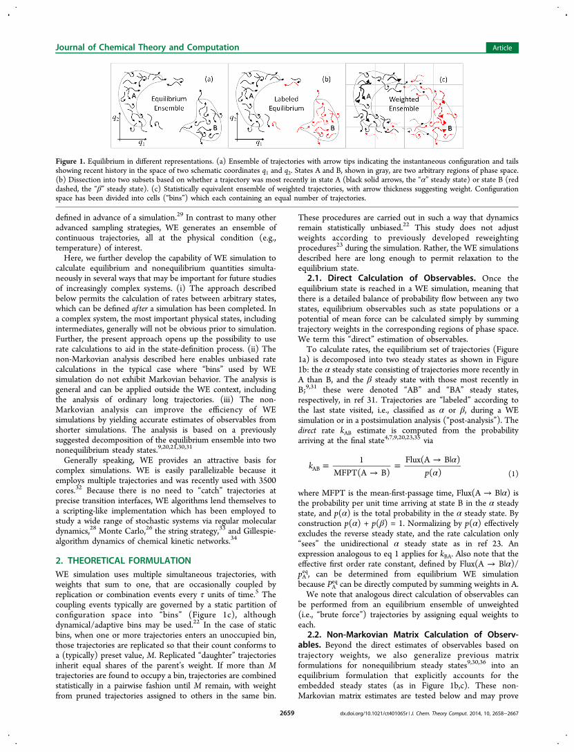
Figure 1. Equilibrium in different representations. (a) Ensemble of trajectories with arrow tips indicating the instantaneous configuration and tailsshowing recent history in the space of two schematic coordinates q1 and q2. States A and B, shown in gray, are two arbitrary regions of phase space.(b) Dissection into two subsets based on whether a trajectory was most recently in state A (black solid arrows, the “α” steady state) or state B (reddashed, the “β” steady state). (c) Statistically equivalent ensemble of weighted trajectories, with arrow thickness suggesting weight. Configurationspace has been divided into cells (“bins”) which each containing an equal number of trajectories.

Journal of Chemical Theory and Computation Article

dx.doi.org/10.1021/ct401065r | J. Chem. Theory Comput. 2014, 10, 2658−26672659

important for future WE studies using shorter simulations, asdescribed in the Discussion.Our matrix approach explicitly uses the decomposition of the

equilibrium population into α and β components for each bin i:

= +α βp p pi i ieq

(2)

which implies p(α) = ∑ipiα and p(β) = ∑ipi

β. We called this a“labeled” analysis. Thus, with N bins, a set of 2N probabilities isrequired rather than N. Similarly, a 2N × 2N rate matrix isrequired: kij

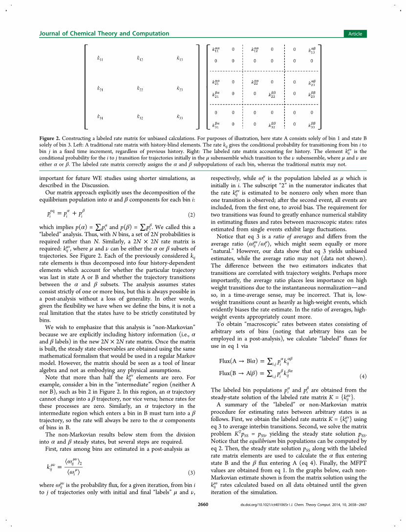
μv, where μ and ν can be either the α or β subsets oftrajectories. See Figure 2. Each of the previously considered kijrate elements is thus decomposed into four history-dependentelements which account for whether the particular trajectorywas last in state A or B and whether the trajectory transitionsbetween the α and β subsets. The analysis assumes statesconsist strictly of one or more bins, but this is always possible ina post-analysis without a loss of generality. In other words,given the flexibility we have when we define the bins, it is not areal limitation that the states have to be strictly constituted bybins.We wish to emphasize that this analysis is “non-Markovian”

because we are explicitly including history information (i.e., αand β labels) in the new 2N × 2N rate matrix. Once the matrixis built, the steady state observables are obtained using the samemathematical formalism that would be used in a regular Markovmodel. However, the matrix should be seen as a tool of linearalgebra and not as embodying any physical assumptions.Note that more than half the kij

μv elements are zero. Forexample, consider a bin in the “intermediate” region (neither Anor B), such as bin 2 in Figure 2. In this region, an α trajectorycannot change into a β trajectory, nor vice versa; hence rates forthese processes are zero. Similarly, an α trajectory in theintermediate region which enters a bin in B must turn into a βtrajectory, so the rate will always be zero to the α componentsof bins in B.The non-Markovian results below stem from the division

into α and β steady states, but several steps are required.First, rates among bins are estimated in a post-analysis as

ω

ω=

⟨ ⟩⟨ ⟩

μνμν

μkijij

i

2

(3)

where ωijμν is the probability flux, for a given iteration, from bin i

to j of trajectories only with initial and final “labels” μ and ν,

respectively, while ωiμ is the population labeled as μ which is

initially in i. The subscript “2” in the numerator indicates thatthe rate kij

μv is estimated to be nonzero only when more thanone transition is observed; after the second event, all events areincluded, from the first one, to avoid bias. The requirement fortwo transitions was found to greatly enhance numerical stabilityin estimating fluxes and rates between macroscopic states: ratesestimated from single events exhibit large fluctuations.Notice that eq 3 is a ratio of averages and differs from the

average ratio ⟨ωijμν/ωi

μ⟩, which might seem equally or more“natural.” However, our data show that eq 3 yields unbiasedestimates, while the average ratio may not (data not shown).The difference between the two estimators indicates thattransitions are correlated with trajectory weights. Perhaps moreimportantly, the average ratio places less importance on highweight transitions due to the instantaneous normalizationandso, in a time-average sense, may be incorrect. That is, low-weight transitions count as heavily as high-weight events, whichevidently biases the rate estimate. In the ratio of averages, high-weight events appropriately count more.To obtain “macroscopic” rates between states consisting of

arbitrary sets of bins (noting that arbitrary bins can beemployed in a post-analysis), we calculate “labeled” fluxes foruse in eq 1 via

α

β

→ | = ∑

→ | = ∑

α αβ

β βα

p k

p k

Flux(A B )

Flux(B A )i j i ij

i j i ij

,

, (4)

The labeled bin populations piα and pi

β are obtained from thesteady-state solution of the labeled rate matrix K = {kij

μν}.A summary of the “labeled” or non-Markovian matrix

procedure for estimating rates between arbitrary states is asfollows. First, we obtain the labeled rate matrix K = {kij

μv} usingeq 3 to average interbin transitions. Second, we solve the matrixproblem KTpSS = pSS, yielding the steady state solution pSS.Notice that the equilibrium bin populations can be computed byeq 2. Then, the steady state solution pSS along with the labeledrate matrix elements are used to calculate the α flux enteringstate B and the β flux entering A (eq 4). Finally, the MFPTvalues are obtained from eq 1. In the graphs below, each non-Markovian estimate shown is from the matrix solution using thekijμν rates calculated based on all data obtained until the giveniteration of the simulation.

Figure 2. Constructing a labeled rate matrix for unbiased calculations. For purposes of illustration, here state A consists solely of bin 1 and state Bsolely of bin 3. Left: A traditional rate matrix with history-blind elements. The rate kij gives the conditional probability for transitioning from bin i tobin j in a fixed time increment, regardless of previous history. Right: The labeled rate matrix accounting for history. The element kij

μv is theconditional probability for the i to j transition for trajectories initially in the μ subensemble which transition to the ν subensemble, where μ and ν areeither α or β. The labeled rate matrix correctly assigns the α and β subpopulations of each bin, whereas the traditional matrix may not.



The non-Markovian matrix formulation exhibits a number ofdesirable properties: (i) Unlike with unlabeled (i.e., implicitlyMarkovian) analysis, kinetic properties will be unbiased asshown below. (ii) Solution of both the α and β steady states isperformed simultaneously via a standard Markov-state-likeanalysis of the kij

μν rate matrix. By contrast, if the α and β steadystates are independently solved within a Markov formalism,there can be substantial ambiguity in how to assign feedbackfrom the target to initial state when the initial state consists ofmore than one bin. (iii) The labeled formulation guarantees, byconstruction, the flux balance intrinsic to equilibrium, namely,Flux(A → B|α) = Flux(B → A|β). (iv) The analysis can beperformed using arbitrary bins (and states defined as sets ofthese bins). It is not necessary to employ the bins originallyused to run the WE simulation because a post-analysis cancalculate rates among any regions of configuration space. (v)The analysis is equally applicable to ordinary brute-forcesimulations.2.3. Markovian Matrix Calculation of Observables. For

reference, we also perform a traditional Markov analysis of thetrajectories, which will prove to yield biased rate estimatesbecause most divisions of configuration space (e.g., WE bins)are not true Markovian states.The Markov analysis proceeds without labeling the

trajectories. Elements of the rate matrix are estimated as

= ⟨ ⟩ ⟨ ⟩k w w/ij ij i2 (5)

where the subscript “2” again means that we only estimate arate as nonzero once at least two transitions from i to j haveoccurred. Bin populations are then computed by solving for thesteady-state solution of the Markov matrix with elements kij.The computation of an MFPT requires the use of source (A)

and sink (B) states. This task is automatically performed withinthe labeled formalism previously described. Hence, wedetermine Markovian macroscopic rates by substituting theMarkovian kij for all nonzero elements of the kij

μν. We emphasizethat this is merely an accounting trick to establish sources andsinks and simultaneously measure both A-to-B and B-to-Afluxes/rates.We perform a smoothing operation on the macroscopic

Markovian rates because otherwise the data are fairly noisy. TheMFPT results shown for the Markovian matrix analysis arerunning averages based on the last 50% of the estimates (whereeach estimate is from the matrix solution using kij estimatesfrom all data obtained until the particular iteration). Weconfirmed numerically that such smoothing did not contributebias to any of the MFPT estimates.

3. MODEL SYSTEMS AND SIMULATION DETAILS

Weighted ensemble simulations were performed on twosystems: the alanine tetrapeptide (Ala4) solvated implicitlyand a pair of explicitly solvated methane molecules. Allsimulations were performed at 300 K with a stochasticthermostat (Langevin thermostat). Friction constants of 5.0and 1.0 ps−1 were used for Ala4 and methane systems,respectively. The molecular dynamics time step used for allsystems was Δt = 2 fs. An iteration is defined to be thesimultaneous propagation of all trajectories in the ensemble forsome amount of time, τ. In these studies, a value of τ = 2500Δtis used for Ala4 and τ = 250Δt for the methane−methanesystem.

For Ala4, the all-atom AMBER ff99SB force field37 withimplicit GB/SA solvent and no cutoff for the evaluation ofnonbonded interactions was simulated using the AMBER 11software package.38 The Hawkins, Cramer, and Truhlar39,40

pairwise generalized Born model is used, with parametersdescribed by Tsui and Case41 (option igb=1 in AMBER 11input file). The progress coordinates were selected and“binned” using a 10 × 10 partition of a 2D space. A dihedraldistance D = ((1/N)∑idi

2)1/2 ∈ [0,180] with respect to areference set of torsions is used in the first dimension, where Nis the number of torsional angles considered and di is thecircular distance between the current value of the ith angle andour reference, i.e., the smaller of the two arclengths along thecircumference. This dimension was divided every 14° from 0 to126° and then a final partition covering the space (126,180]).In the second dimension, a regular RMSD, using only heavyatoms, is measured with respect to an α-helical structure. In thiscase, the space was divided every 0.4 Å from 0 to 3.6 Å andthen a final partition covering the space [3.6,∞). Values andcoordinates for the references used to compute the orderparameters are given in the Supporting Information (SI).The methane molecules were simulated using the GRO-

MACS 4.5 software package42 with the united-atom GROMOS45a3 force field43 and dodecahedral periodic box of TIP3Pwater molecules44 (about 900 water molecules in a 34 × 34 ×24 Å box). van der Waals interactions were switched offsmoothly between 8 and 9 Å; real-space electrostaticinteractions were truncated at 10 Å. Long range electrostaticinteractions were calculated using particle mesh Ewald (PME)summation. The single progress coordinate was the distance rbetween the two methane molecules, following ref 28. Thecoordinate r ∈ [0,∞) Å was partitioned with a bin spacing of 1Å from 0 to 16 Å and a last bin covering the space r ∈ [16,∞)Å.For the post analysis of methane, different bins were used to

demonstrate the flexibility of the approach. The coordinate r ∈[0,∞) Å was partitioned so that the first bin is the space r ∈[0,5) Å, then a bin spacing of 2 Å was used from 5 to 17, whilethe last bin covers the space r ∈ [17,∞) Å.The results shown below include all data generated in all

trajectories: no transient or relaxation period has been omitted.

4. RESULTS

4.1. Ala4. For Ala4, populations and MFPTs are estimatedusing WE and compared to independent measurements basedon ordinary “brute force” (BF) simulation. Rates are estimatedin both directions between the two sets of states A1,B1 andA2,B2 shown in Figure 3 (see SI to visualize representativestructures). The second set is less populated and consequentlyexpected to be more difficult to sample. Figure 3 also shows thebin definitions used in the post-analysis, which were the sameas those used during the WE simulation. However, as we shallsee in our second system, we can use any partition of the spacefor the post analysis.The data shown below are based on the same total

simulation times in BF and WE. The BF estimates andconfidence intervals are based on a single long trajectory of 3.0μs where thousands of transitions between states wereobserved. Five independent WE simulations were run, eachemploying a total of 3.0 μs accounting for all the trajectories.The use of independent WE runs permits straightforward erroranalysis for comparison with BF.



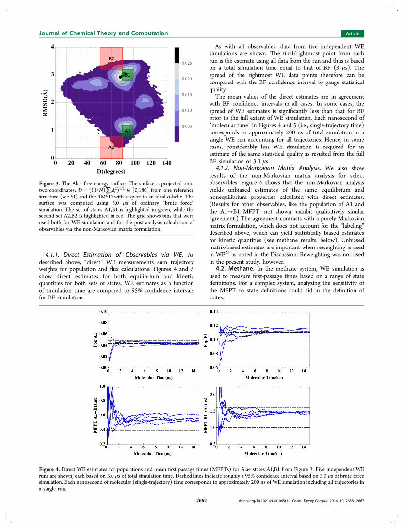
4.1.1. Direct Estimation of Observables via WE. Asdescribed above, “direct” WE measurements sum trajectoryweights for population and flux calculations. Figures 4 and 5show direct estimates for both equilibrium and kineticquantities for both sets of states. WE estimates as a functionof simulation time are compared to 95% confidence intervalsfor BF simulation.

As with all observables, data from five independent WEsimulations are shown. The final/rightmost point from eachrun is the estimate using all data from the run and thus is basedon a total simulation time equal to that of BF (3 μs). Thespread of the rightmost WE data points therefore can becompared with the BF confidence interval to gauge statisticalquality.The mean values of the direct estimates are in agreement

with BF confidence intervals in all cases. In some cases, thespread of WE estimates is significantly less than that for BFprior to the full extent of WE simulation. Each nanosecond of“molecular time” in Figures 4 and 5 (i.e., single-trajectory time)corresponds to approximately 200 ns of total simulation in asingle WE run accounting for all trajectories. Hence, in somecases, considerably less WE simulation is required for anestimate of the same statistical quality as resulted from the fullBF simulation of 3.0 μs.

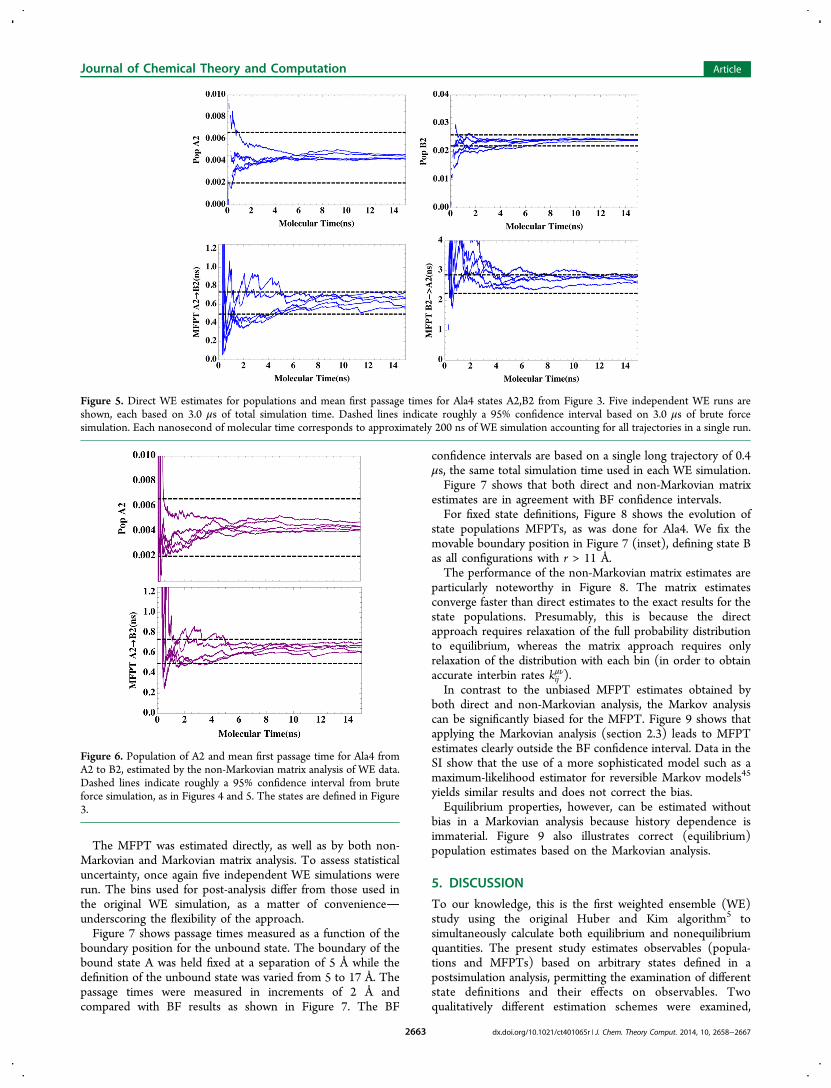
4.1.2. Non-Markovian Matrix Analysis. We also showresults of the non-Markovian matrix analysis for selectobservables. Figure 6 shows that the non-Markovian analysisyields unbiased estimates of the same equilibrium andnonequilibrium properties calculated with direct estimates.(Results for other observables, like the population of A1 andthe A1→B1 MFPT, not shown, exhibit qualitatively similaragreement.) The agreement contrasts with a purely Markovianmatrix formulation, which does not account for the “labeling”described above, which can yield statistically biased estimatesfor kinetic quantities (see methane results, below). Unbiasedmatrix-based estimates are important when reweighting is usedin WE23 as noted in the Discussion. Reweighting was not usedin the present study, however.

4.2. Methane. In the methane system, WE simulation isused to measure first-passage times based on a range of statedefinitions. For a complex system, analyzing the sensitivity ofthe MFPT to state definitions could aid in the definition ofstates.

Figure 3. The Ala4 free energy surface. The surface is projected ontotwo coordinates: D = ((1/N)∑idi

2)1/2 ∈ [0,180] from one referencestructure (see SI) and the RMSD with respect to an ideal α-helix. Thesurface was computed using 3.0 μs of ordinary “brute force”simulation. The set of states A1,B1 is highlighted in green, while thesecond set A2,B2 is highlighted in red. The grid shows bins that wereused both for WE simulation and for the post-analysis calculation ofobservables via the non-Markovian matrix formulation.

Figure 4. Direct WE estimates for populations and mean first passage times (MFPTs) for Ala4 states A1,B1 from Figure 3. Five independent WEruns are shown, each based on 3.0 μs of total simulation time. Dashed lines indicate roughly a 95% confidence interval based on 3.0 μs of brute forcesimulation. Each nanosecond of molecular (single-trajectory) time corresponds to approximately 200 ns of WE simulation including all trajectories ina single run.



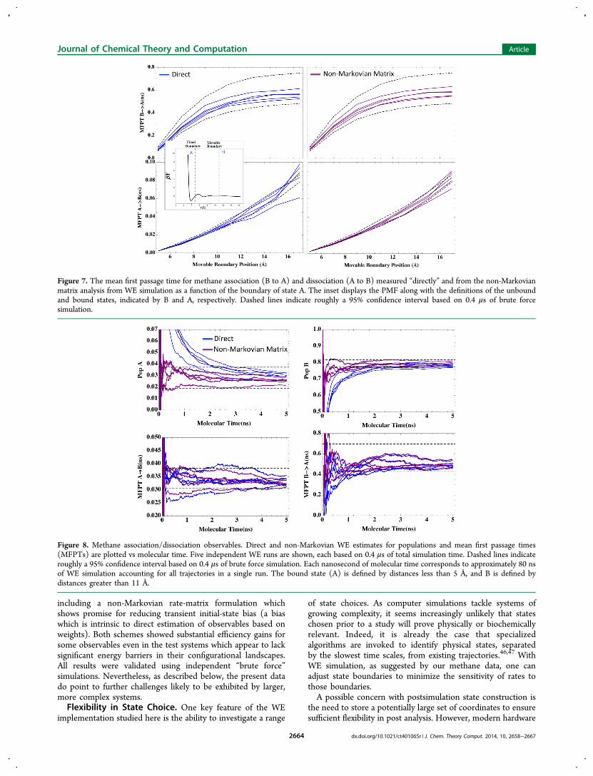
The MFPT was estimated directly, as well as by both non-Markovian and Markovian matrix analysis. To assess statisticaluncertainty, once again five independent WE simulations wererun. The bins used for post-analysis differ from those used inthe original WE simulation, as a matter of convenienceunderscoring the flexibility of the approach.Figure 7 shows passage times measured as a function of the

boundary position for the unbound state. The boundary of thebound state A was held fixed at a separation of 5 Å while thedefinition of the unbound state was varied from 5 to 17 Å. Thepassage times were measured in increments of 2 Å andcompared with BF results as shown in Figure 7. The BF

confidence intervals are based on a single long trajectory of 0.4μs, the same total simulation time used in each WE simulation.Figure 7 shows that both direct and non-Markovian matrix

estimates are in agreement with BF confidence intervals.For fixed state definitions, Figure 8 shows the evolution of

state populations MFPTs, as was done for Ala4. We fix themovable boundary position in Figure 7 (inset), defining state Bas all configurations with r > 11 Å.The performance of the non-Markovian matrix estimates are

particularly noteworthy in Figure 8. The matrix estimatesconverge faster than direct estimates to the exact results for thestate populations. Presumably, this is because the directapproach requires relaxation of the full probability distributionto equilibrium, whereas the matrix approach requires onlyrelaxation of the distribution with each bin (in order to obtainaccurate interbin rates kij

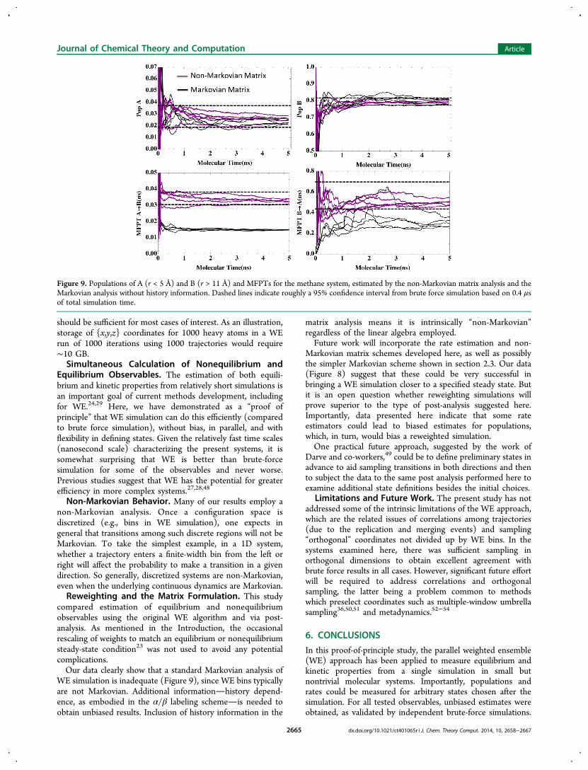
μν).In contrast to the unbiased MFPT estimates obtained by

both direct and non-Markovian analysis, the Markov analysiscan be significantly biased for the MFPT. Figure 9 shows thatapplying the Markovian analysis (section 2.3) leads to MFPTestimates clearly outside the BF confidence interval. Data in theSI show that the use of a more sophisticated model such as amaximum-likelihood estimator for reversible Markov models45

yields similar results and does not correct the bias.Equilibrium properties, however, can be estimated without

bias in a Markovian analysis because history dependence isimmaterial. Figure 9 also illustrates correct (equilibrium)population estimates based on the Markovian analysis.

5. DISCUSSION

To our knowledge, this is the first weighted ensemble (WE)study using the original Huber and Kim algorithm5 tosimultaneously calculate both equilibrium and nonequilibriumquantities. The present study estimates observables (popula-tions and MFPTs) based on arbitrary states defined in apostsimulation analysis, permitting the examination of differentstate definitions and their effects on observables. Twoqualitatively different estimation schemes were examined,

Figure 5. Direct WE estimates for populations and mean first passage times for Ala4 states A2,B2 from Figure 3. Five independent WE runs areshown, each based on 3.0 μs of total simulation time. Dashed lines indicate roughly a 95% confidence interval based on 3.0 μs of brute forcesimulation. Each nanosecond of molecular time corresponds to approximately 200 ns of WE simulation accounting for all trajectories in a single run.

Figure 6. Population of A2 and mean first passage time for Ala4 fromA2 to B2, estimated by the non-Markovian matrix analysis of WE data.Dashed lines indicate roughly a 95% confidence interval from bruteforce simulation, as in Figures 4 and 5. The states are defined in Figure3.



including a non-Markovian rate-matrix formulation whichshows promise for reducing transient initial-state bias (a biaswhich is intrinsic to direct estimation of observables based onweights). Both schemes showed substantial efficiency gains forsome observables even in the test systems which appear to lacksignificant energy barriers in their configurational landscapes.All results were validated using independent “brute force”simulations. Nevertheless, as described below, the present datado point to further challenges likely to be exhibited by larger,more complex systems.Flexibility in State Choice. One key feature of the WE

implementation studied here is the ability to investigate a range

of state choices. As computer simulations tackle systems ofgrowing complexity, it seems increasingly unlikely that stateschosen prior to a study will prove physically or biochemicallyrelevant. Indeed, it is already the case that specializedalgorithms are invoked to identify physical states, separatedby the slowest time scales, from existing trajectories.46,47 WithWE simulation, as suggested by our methane data, one canadjust state boundaries to minimize the sensitivity of rates tothose boundaries.A possible concern with postsimulation state construction is

the need to store a potentially large set of coordinates to ensuresufficient flexibility in post analysis. However, modern hardware

Figure 7. The mean first passage time for methane association (B to A) and dissociation (A to B) measured “directly” and from the non-Markovianmatrix analysis from WE simulation as a function of the boundary of state A. The inset displays the PMF along with the definitions of the unboundand bound states, indicated by B and A, respectively. Dashed lines indicate roughly a 95% confidence interval based on 0.4 μs of brute forcesimulation.

Figure 8. Methane association/dissociation observables. Direct and non-Markovian WE estimates for populations and mean first passage times(MFPTs) are plotted vs molecular time. Five independent WE runs are shown, each based on 0.4 μs of total simulation time. Dashed lines indicateroughly a 95% confidence interval based on 0.4 μs of brute force simulation. Each nanosecond of molecular time corresponds to approximately 80 nsof WE simulation accounting for all trajectories in a single run. The bound state (A) is defined by distances less than 5 Å, and B is defined bydistances greater than 11 Å.



should be sufficient for most cases of interest. As an illustration,storage of {x,y,z} coordinates for 1000 heavy atoms in a WErun of 1000 iterations using 1000 trajectories would require∼10 GB.Simultaneous Calculation of Nonequilibrium and

Equilibrium Observables. The estimation of both equili-brium and kinetic properties from relatively short simulations isan important goal of current methods development, includingfor WE.24,29 Here, we have demonstrated as a “proof ofprinciple” that WE simulation can do this efficiently (comparedto brute force simulation), without bias, in parallel, and withflexibility in defining states. Given the relatively fast time scales(nanosecond scale) characterizing the present systems, it issomewhat surprising that WE is better than brute-forcesimulation for some of the observables and never worse.Previous studies suggest that WE has the potential for greaterefficiency in more complex systems.27,28,48

Non-Markovian Behavior. Many of our results employ anon-Markovian analysis. Once a configuration space isdiscretized (e.g., bins in WE simulation), one expects ingeneral that transitions among such discrete regions will not beMarkovian. To take the simplest example, in a 1D system,whether a trajectory enters a finite-width bin from the left orright will affect the probability to make a transition in a givendirection. So generally, discretized systems are non-Markovian,even when the underlying continuous dynamics are Markovian.Reweighting and the Matrix Formulation. This study

compared estimation of equilibrium and nonequilibriumobservables using the original WE algorithm and via post-analysis. As mentioned in the Introduction, the occasionalrescaling of weights to match an equilibrium or nonequilibriumsteady-state condition23 was not used to avoid any potentialcomplications.Our data clearly show that a standard Markovian analysis of

WE simulation is inadequate (Figure 9), since WE bins typicallyare not Markovian. Additional informationhistory depend-ence, as embodied in the α/β labeling schemeis needed toobtain unbiased results. Inclusion of history information in the

matrix analysis means it is intrinsically “non-Markovian”regardless of the linear algebra employed.Future work will incorporate the rate estimation and non-

Markovian matrix schemes developed here, as well as possiblythe simpler Markovian scheme shown in section 2.3. Our data(Figure 8) suggest that these could be very successful inbringing a WE simulation closer to a specified steady state. Butit is an open question whether reweighting simulations willprove superior to the type of post-analysis suggested here.Importantly, data presented here indicate that some rateestimators could lead to biased estimates for populations,which, in turn, would bias a reweighted simulation.One practical future approach, suggested by the work of

Darve and co-workers,49 could be to define preliminary states inadvance to aid sampling transitions in both directions and thento subject the data to the same post analysis performed here toexamine additional state definitions besides the initial choices.

Limitations and Future Work. The present study has notaddressed some of the intrinsic limitations of the WE approach,which are the related issues of correlations among trajectories(due to the replication and merging events) and sampling“orthogonal” coordinates not divided up by WE bins. In thesystems examined here, there was sufficient sampling inorthogonal dimensions to obtain excellent agreement withbrute force results in all cases. However, significant future effortwill be required to address correlations and orthogonalsampling, the latter being a problem common to methodswhich preselect coordinates such as multiple-window umbrellasampling36,50,51 and metadynamics.52−54

6. CONCLUSIONS

In this proof-of-principle study, the parallel weighted ensemble(WE) approach has been applied to measure equilibrium andkinetic properties from a single simulation in small butnontrivial molecular systems. Importantly, populations andrates could be measured for arbitrary states chosen after thesimulation. For all tested observables, unbiased estimates wereobtained, as validated by independent brute-force simulations.

Figure 9. Populations of A (r < 5 Å) and B (r > 11 Å) and MFPTs for the methane system, estimated by the non-Markovian matrix analysis and theMarkovian analysis without history information. Dashed lines indicate roughly a 95% confidence interval from brute force simulation based on 0.4 μsof total simulation time.



In a number of instances, WE was significantly more efficientyielding estimates of a given statistical quality in less overallcomputing time compared to simple simulation, including alltrajectories. In this sense, not only is WE a parallel method butit can exhibit “super-linear scaling;” e.g., 100 cores can yielddesired information more than 100 times faster than single-coresimulation.We also developed a non-Markovian matrix approach for

analyzing WE or brute-force trajectories, capable of yieldingunbiased results, sometimes faster than direct estimates ofobservables from WE. The non-Markovian formulation alsoyields simultaneous estimates of equilibrium and nonequili-brium observables based on an arbitrary division of phase space,which is not possible in a standard Markovian analysis.The approaches tested here will need to be further developed

and tested in more complex systems.

■ ASSOCIATED CONTENT*S Supporting InformationReference coordinates for the order parameters in Ala4,visualization of the states used in Ala4 (A1, A2, B1, and B2),and a comparison of the regular Markov model vs theMaximum Likelihood Estimator for reversible Markov modelsare shown. This material is available free of charge via theInternet at http://pubs.acs.org/.

■ AUTHOR INFORMATIONCorresponding Author*E-mail: [email protected].

Author Contributions∥Equal contributions

NotesThe authors declare no competing financial interest.

■ ACKNOWLEDGMENTSWe thank Josh Adelman for insightful discussions, as well as thefinancial support from the NIH (Grant No. P41 GM103712)and the NSF (Grant Nos. MCB-0643456, MCB-1119091 andMCB- 0845216).

■ REFERENCES(1) Berg, J. M.; Tymoczko, J. L.; Stryer, L. Biochemistry, 5th ed.;Freeman: New York, 2002.(2) Zuckerman, D. M. Annu Rev. Biophys. 2011, 40, 41−62.(3) Swendsen, R. H.; Wang, J.-S. Phys. Rev. Lett. 1986, 57, 2607−2609.(4) Zheng, L.; Chen, M.; Yang, W. Proc. Natl. Acad. Sci. U. S. A. 2008,105, 20227−20232.(5) Huber, G. A.; Kim, S. Biophys. J. 1996, 70, 97−110.(6) Bolhuis, P. G.; Chandler, D.; Dellago, C.; Geissler, P. L. Annu.Rev. Phys. Chem. 2002, 53, 291−318.(7) Allen, R. J.; Warren, P. B.; ten Wolde, P. R. Phys. Rev. Lett. 2005,94, No. 018104.(8) Warmflash, A.; Bhimalapuram, P.; Dinner, A. R. J. Chem. Phys.2007, 127, 154112−8.(9) Vanden-Eijnden, E.; Venturoli, M. J. Chem. Phys. 2009, 131,No. 044120.(10) Faradjian, A. K.; Elber, R. J. Chem. Phys. 2004, 120, 10880−10889.(11) Shaw, D. E.; Maragakis, P.; Lindorff-Larsen, K.; Piana, S.; Dror,R. O.; Eastwood, M. P.; Bank, J. A.; Jumper, J. M.; Salmon, J. K.; Shan,Y.; Wriggers, W. Science 2010, 330, 341−346.(12) Sugita, Y.; Okamoto, Y. Chem. Phys. Lett. 1999, 314, 141.

(13) Buchete, N.-V.; Hummer, G. Phys. Rev. E: Stat. Nonlin. SoftMatter Phys. 2008, 77, 030902.(14) Huang, X.; Bowman, G. R.; Bacallado, S.; Pande, V. S. Proc. Natl.Acad. Sci. U. S. A. 2009, 106, 19765−19769.(15) Noe, F.; Schtte, C.; Vanden-Eijnden, E.; Reich, L.; Weikl, T. R.Proc. Natl. Acad. Sci. U. S. A. 2009, 106, 19011−19016.(16) Faradjian, A. K.; Elber, R. J. Chem. Phys. 2004, 120, 10880−10889.(17) West, A. M. A.; Elber, R.; Shalloway, D. J. Chem. Phys. 2007,126, 145104−14.(18) van Erp, T. S.; Moroni, D.; Bolhuis, P. G. J. Chem. Phys. 2003,118, 7762−7774.(19) Moroni, D.; Bolhuis, P. G.; van Erp, T. S. J. Chem. Phys. 2004,120, 4055−4065.(20) Moroni, D.; van Erp, T. S.; Bolhuis, P. G. Phys. Rev. E: Stat.,Nonlinear, Soft Matter Phys. 2005, 71, 056709.(21) Valeriani, C.; Allen, R. J.; Morelli, M. J.; Frenkel, D.; ten Wolde,P. R. J. Chem. Phys. 2007, 127, 114109.(22) Zhang, B. W.; Jasnow, D.; Zuckerman, D. M. J. Chem. Phys.2010, 132, 054107.(23) Bhatt, D.; Zhang, B. W.; Zuckerman, D. M. J. Chem. Phys. 2010,133, 014110.(24) Bhatt, D.; Bahar, I. J. Chem. Phys. 2012, 137, 104101.(25) Rojnuckarin, A.; Kim, S.; Subramaniam, S. Proc. Natl. Acad. Sci.U. S. A. 1998, 95, 4288−4292.(26) Zhang, B. W.; Jasnow, D.; Zuckerman, D. M. Proc. Natl. Acad.Sci. U. S. A. 2007, 104, 18043−18048.(27) Bhatt, D.; Zuckerman, D. M. J. Chem. Theory Comput. 2010, 6,3527−3539.(28) Zwier, M. C.; Kaus, J. W.; Chong, L. T. J. Chem. Theory Comput.2011, 7, 1189−1197.(29) Darve, E.; Ryu, E. In Innovations in Biomolecular Modeling andSimulations: Vol. 1; Schlick, T., Ed.; Royal Society of Chemistry:London, 2012; Chapter Computing Reaction Rates in Bio-molecularSystems Using Discrete Macro-states, pp 138−206.(30) Dickson, A.; Warmflash, A.; Dinner, A. R. J. Chem. Phys. 2009,131, 154104.(31) Bhatt, D.; Zuckerman, D. M. J. Chem. Theory Comput. 2011, 7,2520−2527. PMCID: PMC3159166.(32) Zwier, M. C.; Kaus, J. W.; Adelman, J. L.; Pratt, A. J.;Zuckerman, D. M.; Chong, L. T. 2014. Manuscript submitted forpublication.(33) Adelman, J. L.; Grabe, M. J. Chem. Phys. 2013, 138, 044105.(34) Donovan, R. M.; Sedgewick, A. J.; Faeder, J. R.; Zuckerman, D.M. J. Chem. Phys. 2013, 139, 115105.(35) Zuckerman, D. M. Statistical Physics of Biomolecules: AnIntroduction; CRC Press: Boca Raton, FL, 2010.(36) Dickson, A.; Maienschein-Cline, M.; Tovo-Dwyer, A.;Hammond, J. R.; Dinner, A. R. J. Chem. Theory Comput. 2011, 7,2710−2720.(37) Hornak, V.; Abel, R.; Okur, A.; Strockbine, B.; Roitberg, A.;Simmerling, C. Proteins 2006, 65, 712−725.(38) Case, D. A.; Darden, T. A.; Cheatham, T. E.; Simmerling, C. L.;Wang, J.; Duke, R. E.; Luo, R.; Crowley, M.; Walker, R. C.; Zhang, W.;Merz, K. M.; Wang, B.; Hayik, S.; Roitberg, A.; Seabra, G.; Kolossvary,I.; Wong, K. F.; Paesani, F.; Vanicek, J.; Wu, X.; Brozell, S. R.;Steinbrecher, T.; Gohlke, H.; Yang, L.; Tan, C.; Mongan, J.; Hornak,V.; Cui, G.; Mathews, D. H.; Seetin, M. G.; Sagui, C.; Babin, V.;Kollman, P. A. Amber 11; University of California: San Francisco.(39) Hawkins, G.; Cramer, C.; Truhlar, D. J. Phys. Chem. 1996, 100,19824−19839.(40) Hawkins, G.; Cramer, C.; Truhlar, D. Chem. Phys. Lett. 1995,246, 122−129.(41) Tsui, V.; Case, D. Biopolymers 2001, 56, 275−291.(42) Hess, B.; Kutzner, C.; van der Spoel, D.; Lindahl, E. J. Chem.Theory Comput. 2008, 4, 435−447.(43) Schuler, L. D.; Daura, X.; Van Gunsteren, W. F. J. Comput.Chem. 2001, 22, 1205−1218.



http://pubs.acs.org/

mailto:[email protected]

(44) Jorgensen, W. L.; Chandrasekhar, J.; Madura, J. D.; Impey, R.W.; Klein, M. L. J. Chem. Phys. 1983, 79, 926−935.(45) Beauchamp, K. A.; Bowman, G. R.; Lane, T. J.; Maibaum, L.;Haque, I. S.; Pande, V. S. J. Chem. Theory Comput. 2011, 7, 3412−3419.(46) Chodera, J. D.; Singhal, N.; Pande, V. S.; Dill, K. A.; Swope, W.C. J. Chem. Phys. 2007, 126, 155101−17.(47) Zhang, X.; Bhatt, D.; Zuckerman, D. M. J. Chem. TheoryComput. 2010, 6, 30483057.(48) Adelman, J. L.; Dale, A. L.; Zwier, M. C.; Bhatt, D.; Chong, L.T.; Zuckerman, D. M.; Grabe, M. Biophys. J. 2011, 101, 2399−2407.(49) Abdul-Wahid, B.; Yu, L.; Rajan, D.; Feng, H.; Darve, E.; Thain,D.; Izaguirre, J. A. Folding proteins at 500 ns/hour with Work Queue.2012 IEEE 8th International Conference on E-Science, e-Science2012.(50) Haydock, C.; Sharp, J. C.; Prendergast, F. G. Biophys. J. 1990,57, 1269−1279.(51) Dickson, A.; Warmflash, A.; Dinner, A. R. J. Chem. Phys. 2009,130, 074104−12.(52) Vargiu, A. V.; Ruggerone, P.; Magistrato, A.; Carloni, P. NucleicAcids Res. 2008, 36, 5910−5921.(53) Bussi, G.; Laio, A.; Parrinello, M. Phys. Rev. Lett. 2006, 96,090601.(54) Raiteri, P.; Laio, A.; Gervasio, F. L.; Micheletti, C.; Parrinello, M.J. Phys. Chem. B 2006, 110, 3533−3539.



simultaneous computation of dynamical and …cstringer/papers/we.pdfsimultaneous computation of...

Documents