simulation lecture 8 - faculteit wiskunde en informaticamarko/2wb05/lecture8.pdf · 2wb05...

2WB05 SimulationLecture 8: Generatingrandom variables

Marko Boonhttp://www.win.tue.nl/courses/2WB05

January 7, 2013

2/36

Department of Mathematics and Computer Science

1. How do we generate random variables?

2. Fitting distributions

Outline

3/36


How do we generate random variables?• Sampling from continuous distributions

• Sampling from discrete distributions

Generating random variables

4/36


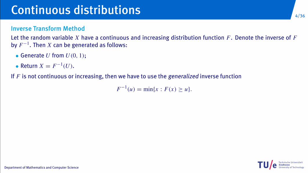
Inverse Transform MethodLet the random variable X have a continuous and increasing distribution function F . Denote the inverse of Fby F−1. Then X can be generated as follows:

• Generate U from U (0, 1);

• Return X = F−1(U ).

If F is not continuous or increasing, then we have to use the generalized inverse function

F−1(u) = min{x : F(x) ≥ u}.

Continuous distributions

5/36


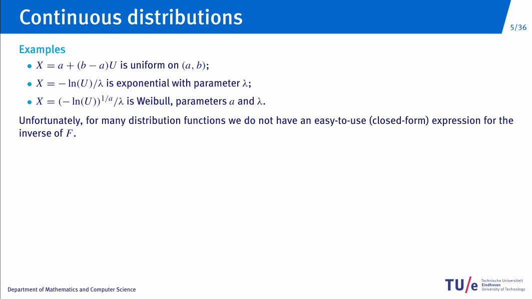
Examples• X = a + (b − a)U is uniform on (a, b);

• X = − ln(U )/λ is exponential with parameter λ;

• X = (− ln(U ))1/a/λ is Weibull, parameters a and λ.

Unfortunately, for many distribution functions we do not have an easy-to-use (closed-form) expression for theinverse of F .


6/36


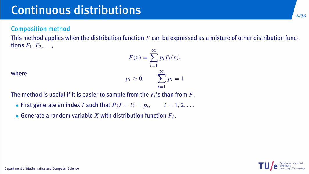
Composition methodThis method applies when the distribution function F can be expressed as a mixture of other distribution func-tions F1, F2, . . .,

F(x) =∞∑

i=1

pi Fi(x),

wherepi ≥ 0,

∞∑i=1

pi = 1

The method is useful if it is easier to sample from the Fi ’s than from F .

• First generate an index I such that P(I = i) = pi , i = 1, 2, . . .

• Generate a random variable X with distribution function FI .


7/36


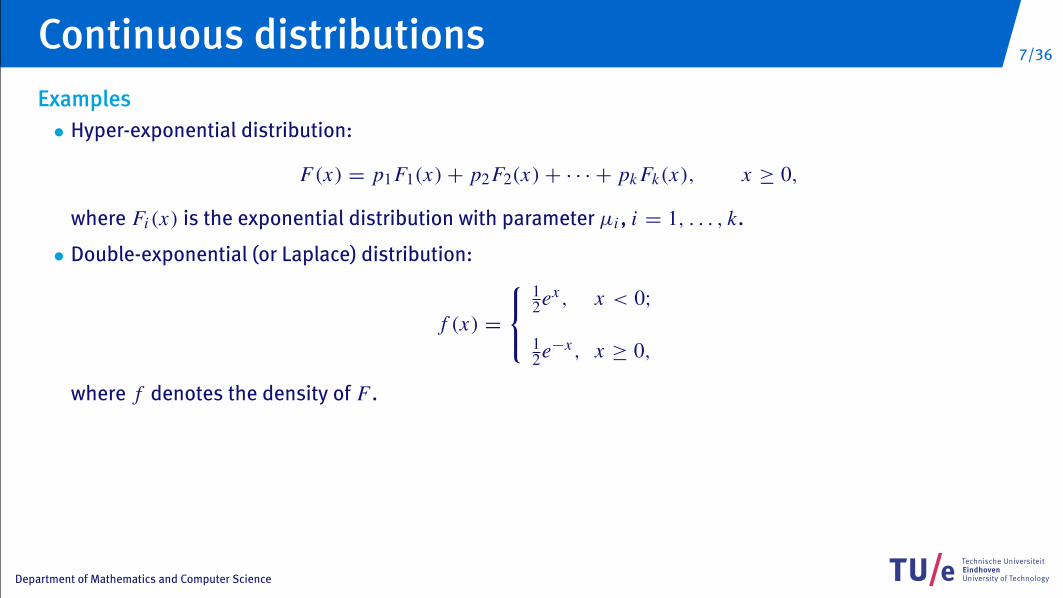
Examples• Hyper-exponential distribution:

F(x) = p1F1(x)+ p2F2(x)+ · · · + pk Fk(x), x ≥ 0,

where Fi(x) is the exponential distribution with parameter µi , i = 1, . . . , k.

• Double-exponential (or Laplace) distribution:

f (x) =

12ex, x < 0;

12e−x, x ≥ 0,

where f denotes the density of F .


8/36


Convolution methodIn some case X can be expressed as a sum of independent random variables Y1, . . . , Yn, so

X = Y1 + Y2 + · · · + Yn.

where the Yi ’s can be generated more easily than X .

Algorithm:

• Generate independent Y1, . . . , Yn, each with distribution function G;

• Return X = Y1 + · · · + Yn.


9/36


ExampleIf X is Erlang distributed with parameters n and µ, then X can be expressed as a sum of n independentexponentials Yi , each with mean 1/µ.

Algorithm:

• Generate n exponentials Y1, . . . , Yn, each withmean µ;

• Set X = Y1 + · · · + Yn.

More efficient algorithm:

• Generate n uniform (0, 1) random variablesU1, . . . ,Un;

• Set X = − ln(U1U2 · · ·Un)/µ.


10/36


Acceptance-Rejection methodDenote the density of X by f . This method requires a function g that majorizes f ,

g(x) ≥ f (x)

for all x . Now g will not be a density, since

c =∫∞

−∞

g(x)dx ≥ 1.

Assume that c <∞. Then h(x) = g(x)/c is a density. Algorithm:

1. Generate Y having density h;

2. Generate U from U (0, 1), independent of Y ;

3. If U ≤ f (Y )/g(Y ), then set X = Y ; else go back to step 1.

The random variable X generated by this algorithm has density f .


11/36


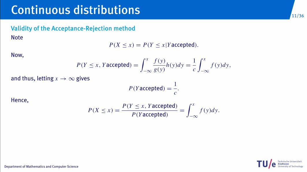
Validity of the Acceptance-Rejection methodNote

P(X ≤ x) = P(Y ≤ x |Y accepted).

Now,

P(Y ≤ x, Y accepted) =∫ x

−∞

f (y)g(y)

h(y)dy =1c

∫ x

−∞

f (y)dy,

and thus, letting x →∞ gives

P(Y accepted) =1c.

Hence,

P(X ≤ x) =P(Y ≤ x, Y accepted)

P(Y accepted)=

∫ x

−∞

f (y)dy.


12/36


Note that the number of iterations is geometrically distributed with mean c.

How to choose g?

• Try to choose g such that the random variable Y can be generated rapidly;

• The probability of rejection in step 3 should be small; so try to bring c close to 1, which mean that g shouldbe close to f .


13/36


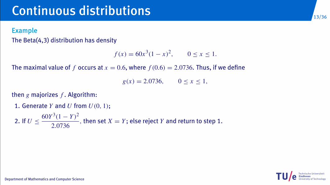
ExampleThe Beta(4,3) distribution has density

f (x) = 60x3(1− x)2, 0 ≤ x ≤ 1.

The maximal value of f occurs at x = 0.6, where f (0.6) = 2.0736. Thus, if we define

g(x) = 2.0736, 0 ≤ x ≤ 1,

then g majorizes f . Algorithm:

1. Generate Y and U from U (0, 1);

2. If U ≤60Y 3(1− Y )2

2.0736, then set X = Y ; else reject Y and return to step 1.


14/36


Normal distributionMethods:

• Acceptance-Rejection method

• Box-Muller method


15/36


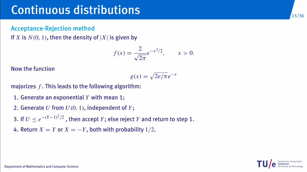
Acceptance-Rejection methodIf X is N (0, 1), then the density of |X | is given by

f (x) =2√

2πe−x2/2, x > 0.

Now the functiong(x) =

√2e/πe−x

majorizes f . This leads to the following algorithm:

1. Generate an exponential Y with mean 1;

2. Generate U from U (0, 1), independent of Y ;

3. If U ≤ e−(Y−1)2/2 , then accept Y ; else reject Y and return to step 1.

4. Return X = Y or X = −Y , both with probability 1/2.


16/36


Box-Muller methodIf U1 and U2 are independent U (0, 1) random variables, then

X1 =√−2 ln U1 cos(2πU2)

X2 =√−2 ln U1 sin(2πU2)

are independent standard normal random variables.

This method is implemented in the function nextGaussian() in java.util.Random


17/36


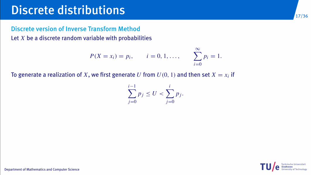
Discrete version of Inverse Transform MethodLet X be a discrete random variable with probabilities

P(X = xi) = pi , i = 0, 1, . . . ,∞∑

i=0

pi = 1.

To generate a realization of X , we first generate U from U (0, 1) and then set X = xi if

i−1∑j=0

p j ≤ U <

i∑j=0

p j .

Discrete distributions

18/36


So the algorithm is as follows:


• Determine the index I such thatI−1∑j=0

p j ≤ U <

I∑j=0

p j

and return X = x I .

The second step requires a search; for example, starting with I = 0 we keep adding 1 to I until we have foundthe (smallest) I such that

U <

I∑j=0

p j

Note: The algorithm needs exactly one uniform random variable U to generate X ; this is a nice feature if youuse variance reduction techniques.


19/36


Array method: when X has a finite supportSuppose pi = ki/100, i = 1, . . . ,m,where ki ’s are integers with 0 ≤ ki ≤ 100

Construct array A[i], i = 1, . . . , 100 as follows:set A[i] = x1 for i = 1, . . . , k1set A[i] = x2 for i = k1 + 1, . . . , k1 + k2, etc.

Then, first sample a random index I from 1, . . . , 100:I = 1+ b100Uc and set X = A[I ]


20/36


BernoulliTwo possible outcomes of X (success or failure):

P(X = 1) = 1− P(X = 0) = p.

Algorithm:


• If U ≤ p, then X = 1; else X = 0.


21/36


Discrete uniformThe possible outcomes of X are m,m + 1, . . . , n and they are all equally likely, so

P(X = i) =1

n − m + 1, i = m,m + 1, . . . , n.

Algorithm:


• Set X = m + b(n − m + 1)Uc.

Note: No search is required, and compute (n − m + 1) ahead.


22/36


GeometricA random variable X has a geometric distribution with parameter p if

P(X = i) = p(1− p)i , i = 0, 1, 2, . . . ;

X is the number of failures till the first success in a sequence of Bernoulli trials with success probability p.

Algorithm:

• Generate independent Bernoulli(p) random variables Y1, Y2, . . .; let I be the index of the first successfulone, so YI = 1;

• Set X = I − 1.

Alternative algorithm:


• Set X = bln(U )/ ln(1− p)c.


23/36


BinomialA random variable X has a binomial distribution with parameters n and p if

P(X = i) =(

ni

)pi(1− p)n−i , i = 0, 1, . . . , n;

X is the number of successes in n independent Bernoulli trials, each with success probability p.

Algorithm:

• Generate n Bernoulli(p) random variablesY1, . . . , Yn;

• Set X = Y1 + Y2 + · · · + Yn.

Alternative algorithms can be derived by using the following results.


24/36


Let Y1, Y2, . . . be independent geometric(p) random variables, and I the smallest index such that

I+1∑i=1

(Yi + 1) > n.

Then the index I has a binomial distribution with parameters n and p.

Let Y1, Y2, . . . be independent exponential random variables with mean 1, and I the smallest index such that

I+1∑i=1

Yi

n − i + 1> − ln(1− p).

Then the index I has a binomial distribution with parameters n and p.


25/36


Negative BinomialA random variable X has a negative-binomial distribution with parameters n and p if

P(X = i) =(

n + i − 1i

)pn(1− p)i , i = 0, 1, 2, . . . ;

X is the number of failures before the n-th success in a sequence of independent Bernoulli trials with successprobability p.

Algorithm:

• Generate n geometric(p) random variablesY1, . . . , Yn;

• Set X = Y1 + Y2 + · · · + Yn.


26/36


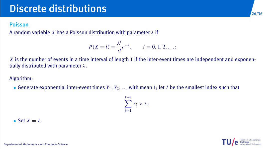
PoissonA random variable X has a Poisson distribution with parameter λ if

P(X = i) =λi

i !e−λ, i = 0, 1, 2, . . . ;

X is the number of events in a time interval of length 1 if the inter-event times are independent and exponen-tially distributed with parameter λ.

Algorithm:

• Generate exponential inter-event times Y1, Y2, . . . with mean 1; let I be the smallest index such that

I+1∑i=1

Yi > λ;

• Set X = I .


27/36


Poisson (alternative)• Generate U(0,1) random variables U1,U2, . . .;

let I be the smallest index such thatI+1∏i=1

Ui < e−λ;

• Set X = I .


28/36


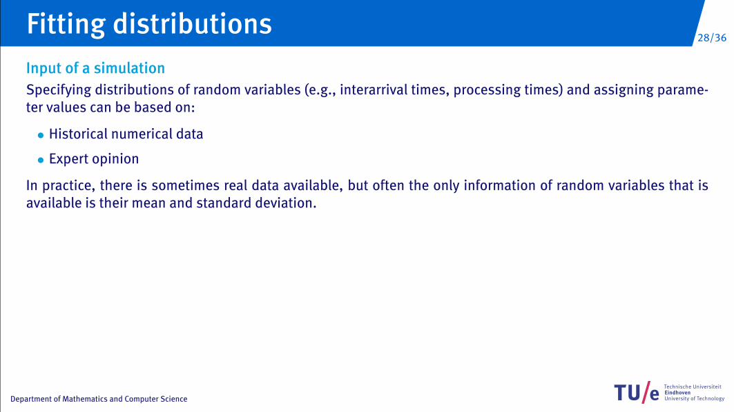
Input of a simulationSpecifying distributions of random variables (e.g., interarrival times, processing times) and assigning parame-ter values can be based on:

• Historical numerical data

• Expert opinion

In practice, there is sometimes real data available, but often the only information of random variables that isavailable is their mean and standard deviation.

Fitting distributions

29/36


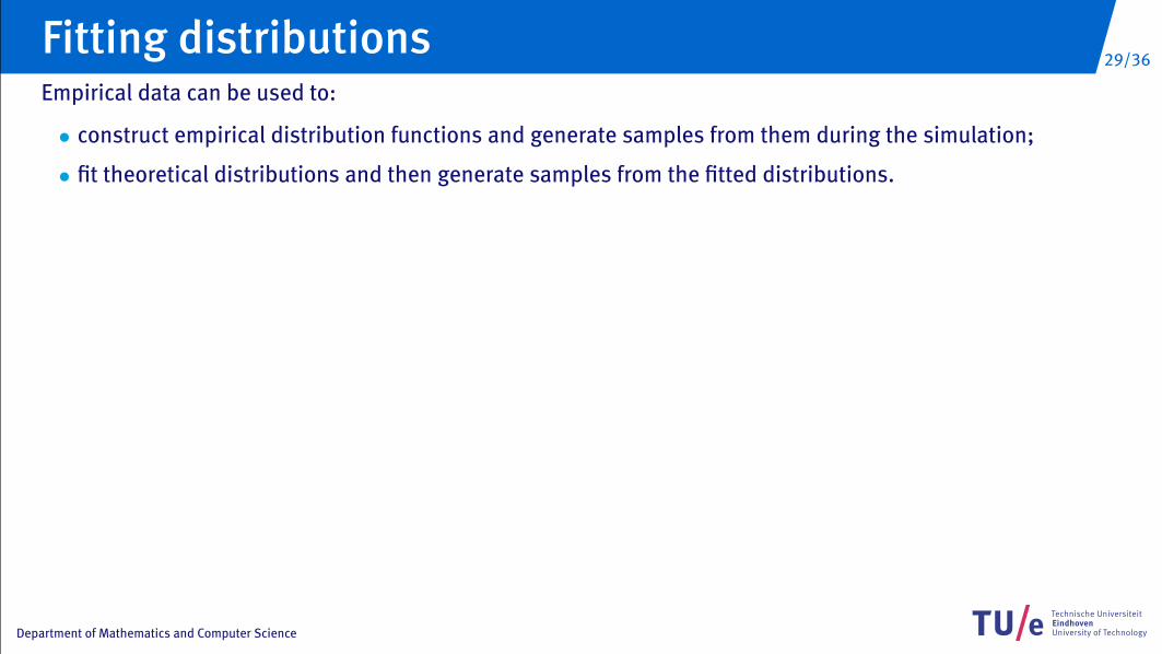
Empirical data can be used to:

• construct empirical distribution functions and generate samples from them during the simulation;

• fit theoretical distributions and then generate samples from the fitted distributions.


30/36


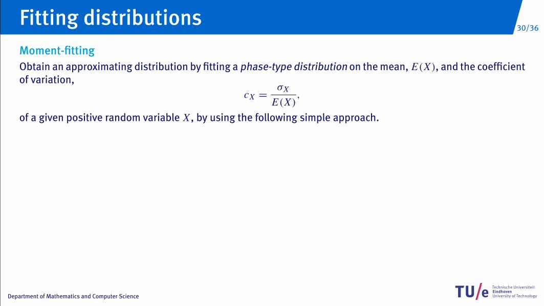
Moment-fittingObtain an approximating distribution by fitting a phase-type distribution on the mean, E(X), and the coefficientof variation,

cX =σX

E(X),

of a given positive random variable X , by using the following simple approach.


31/36


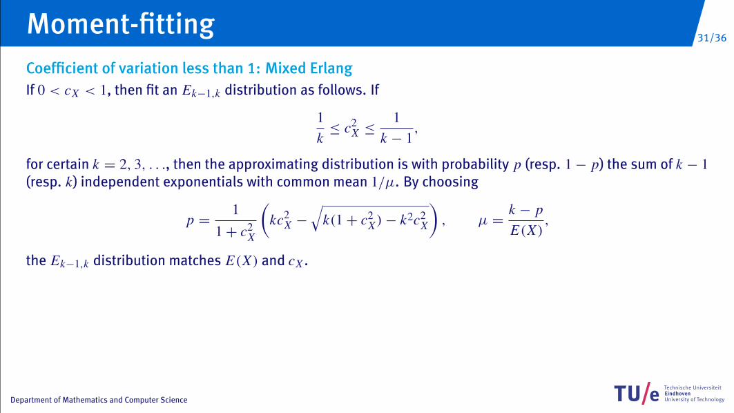
Coefficient of variation less than 1: Mixed ErlangIf 0 < cX < 1, then fit an Ek−1,k distribution as follows. If

1k≤ c2

X ≤1

k − 1,

for certain k = 2, 3, . . ., then the approximating distribution is with probability p (resp. 1− p) the sum of k − 1(resp. k) independent exponentials with common mean 1/µ. By choosing

p =1

1+ c2X

(kc2

X −

√k(1+ c2

X)− k2c2X

), µ =

k − pE(X)

,

the Ek−1,k distribution matches E(X) and cX .

Moment-fitting

32/36


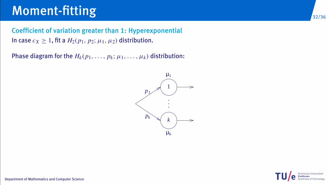
Coefficient of variation greater than 1: HyperexponentialIn case cX ≥ 1, fit a H2(p1, p2;µ1, µ2) distribution.

Phase diagram for the Hk(p1, . . . , pk;µ1, . . . , µk) distribution:

1

k

µ1

µk

p 1

pk

Moment-fitting

33/36


But the H2 distribution is not uniquely determined by its first two moments. In applications, the H2 distributionwith balanced means is often used. This means that the normalization

p1

µ1=

p2

µ2

is used. The parameters of the H2 distribution with balanced means and fitting E(X) and cX (≥ 1) are given by

p1 =12

(1+

√c2

X − 1

c2X + 1

), p2 = 1− p1,

µ1 =2p1

E(X), µ2 =

2p2

E(X).

Moment-fitting

34/36


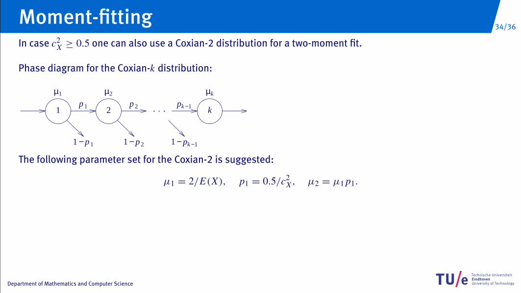
In case c2X ≥ 0.5 one can also use a Coxian-2 distribution for a two-moment fit.

Phase diagram for the Coxian-k distribution:

1 2 k

µ1 µ2 µk

p 1 p 2 pk −1

1 − p 1 1 − p 2 1 − pk −1

The following parameter set for the Coxian-2 is suggested:

µ1 = 2/E(X), p1 = 0.5/c2X , µ2 = µ1 p1.

Moment-fitting

35/36


Fitting nonnegative discrete distributionsLet X be a random variable on the non-negative integers with mean E(X) and coefficient of variation cX . Thenit is possible to fit a discrete distribution on E(X) and cX using the following families of distributions:

• Mixtures of Binomial distributions;

• Poisson distribution;

• Mixtures of Negative-Binomial distributions;

• Mixtures of geometric distributions.

This fitting procedure is described in Adan, van Eenige and Resing (see Probability in the Engineering andInformational Sciences, 9, 1995, pp 623-632).

Moment-fitting

36/36


Adequacy of fit

• Graphical comparison of fitted and empirical curves;

• Statistical tests (goodness-of-fit tests).


simulation lecture 8 - faculteit wiskunde en informaticamarko/2wb05/lecture8.pdf · 2wb05...

Documents