NASA Technical Paper 1122

Simplified Sonic-Boom Prediction

Harry W. Carlson

Langley Research Center

Hampton, Virginia

National Aeronautics

and Space Administration

Scientific and Technical

Information Office

1978

SUMMARY

A simplified method for the calculation of sonic-boom characteristics for

a wide variety of supersonic airplane configurations and spacecraft operating

at altitudes up to 76 km has been developed. Sonlc-boom overpressures and sig-

nature duration may be predicted for the entire affected ground area for vehi-

cles in level flight or in moderate climbing or descending flight paths. The

outlined procedure relies to a great extent on the use of charts to provide

generation and propagation factors for use in relatively simple expressions

for signature calculation. The computational requirements can be met by hand-

held scientific calculators, or even by slide rules. With little sacrifice in

accuracy, complete calculations can often be obtained in less time than is

required for the preparation of computer input data for the more rigorous cal-

culation methods. A variety of correlations of predicted and measured sonic-

boom data for airplanes and spacecraft serve to demonstrate the applicabilityof the simplified method.

INTRODUCTION

As the understanding of sonic-boom phenomena has advanced, and the abil-

ity to provide accurate predictions of sonic-boom phenomena has improved, the

actual prediction process has become quite complex. For conventional air-

plane configurations, the usual procedures as described in references I and 2

call for employment of several sophisticated computer programs covering air-

plane geometry and aerodynamic considerations as well as the wave propagation

aspects of the problem. For spacecraft operating in the sensible atmosphere,

it has become the practice (ref. 3) to rely on wind-tunnel tests of small but

detailed scale models and specialized computer programs for extrapolation of

the data to full-scale conditions. In either case, the process is complex,

lengthy, and expensive and requires the services of one or more skilled prac-titioners of the art.

The results of a recent study indicate that for many purposes (including

the conduct of preliminary engineering studies and the preparation of environ-

mental impact statements), sonic-boom predictions of sufficient accuracy can

be obtained by using a simplified method which does not require a wind tunnel

or elaborate computing equipment. Computational requirements can in fact be

met by hand-held scientific calculators, or even slide rules. In addition,

successful use of the method is not highly dependent on the skill and knowl-

edge of the person performing the calculations.

This prediction technique results from a simplification of the purely

theoretical methods described in references I and 2, which have been shown to

provide quite acceptable estimates of sonic-boom phenomena for a wide range offlight conditions for conventional airplane configurations. A recent wind-

tunnel study (ref. 4) has shown that purely theoretical methods may be applied

to prediction of sonic-boom phenomena for extremely blunt bodies at highsupersonic speeds, provided that propagation distances are large relative to

body dimensions. This finding justifies the use of the simplified method for

spacecraft as well as for conventional airplane configurations.

This report gives a general description of the prediction method, lists

the steps required in the calculation procedure, and provides charts that are

needed in the process. In addition, sample problems are presented to illus-

trate the method in use, and correlations with flight-test experimental data

are shown to demonstrate its applicability.

The reader interested only in prediction of ground-track overpressures

for conventional airplane configurations may wish to go directly to the sec-

tion entitled "Further Simplification," in which a brief, self-contained pre-

diction method is described.

SYMBOLS

A(x) area of aircraft cross sections normal to flight direction at a

given value of x-coordinate (cross sections normal to longitudinal

axis of aircraft may be substituted in most cases), m2

Ae(X) total effective area of aircraft at a given value of x-coordinate,

A(x) + B(x), m2

Ae, max

Ae,1

maximum effective area, m2

total effective area at midpoint of effective aircraft

length, Ze, m2

a v

B(x)

Bmax

b(x)

speed of sound at aircraft (vehicle) altitude, m/sec

equivalent cross-sectional area due to lift at a given value of

x-coordinate, m2

maximum equivalent cross-sectional area due to lift, m2

local span of aircraft planform at a given value of x-coordinate, m

d distance between aircraft ground-track position at time of

sonic-boom generation and location of ground impact point (see

fig. 5), km

d x

dy

component of d in direction of aircraft ground track, km

component of d in a direction perpendicular to aircraft ground

track (i.e., in lateral direction), km

dy,c value of dy at lateral limit or cutoff of sonic-boom groundfootprint, km

h altitude of aircraft above ground, hv - hg, km

h e

hg

hv

Kd

Kd,c

Kd,_

KL

Kp

Kp,_

KR

KS

Kt

Kt,_

le

M

Mc

M e

nd

np

nt

P

Ap

effective altitude (see fig. 5), km

altitude of ground above sea level, km

altitude of aircraft (vehicle) above sea level, km

ray-path distance factor

ray-path distance factor for cutoff conditions, M e = M c

ray-path distance factor for an infinite Mach number

lift parameter (see fig. 4)

pressure amplification factor

pressure amplification factor for an infinite Mach number

reflection factor, assumed to be 2.0

aircraft shape factor

signature duration factor

signature duration factor for an infinite Mach number

aircraft characteristic length, normally the fuselage length, m

effective length of aircraft used in determination of aircraft

shape factor, m

aircraft Mach number

aircraft cutoff Mach number below which sonic boom will not reach

ground

aircraft effective Mach number governing sonic-boom atmosphere

propagation characteristics

exponent of Mach number parameter in atmospheric distance factor

curve fit (see eq. (12))

exponent of Mach number parameter in atmospheric pressure ampli-

fication factor curve fit (see eq. (13))

exponent of Mach number parameter in atmospheric signature duration

factor curve fit (see eq. (14))

atmospheric pressure, Pa

incremental pressure due to sonic boom, Pa

APr_ x

Pg

Pv

S

At

W

X

Y

%

incremental pressure at N-wave bow shock, also referred to as bow-

shock overpressure, Pa

atmospheric pressure at ground level, Pa

atmospheric pressure at aircraft (vehicle) altitude, Pa

aircraft planform area, m2

time increment, sec

aircraft weight, kg

distance from aircraft nose measured backward along flight path, m

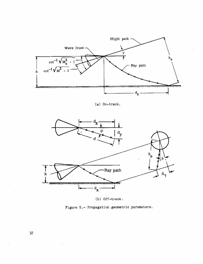
flight-path angle (see fig. 5), deg

ray-path azimuth angle (see fig. 5), deg

angle between aircraft ground track and ground projection of ray

path (see fig. 5), deg

METHOD IN GENERAL

The simplified prediction method is applicable to a wide variety of

supersonic airplane configurations and spacecraft operating at altitudes upto 76 km. It provides estimates of sonic-boom pressure and signature duration

over the entire exposed ground area for vehicles in level flight or in moder-

ate climb or descent flight profiles. The effects of flight-path curvature

and aircraft acceleration, however, are not considered, and the method is

further restricted to a standard atmosphere without winds. These limitations,

however, do not appear to affect the general applicability of the method fornormal variations from the standard atmosphere (temperature profiles and winds)

and for moderate flight-path curvature and aircraft acceleration. When situa-

tions do arise in which these effects are important, Whitham F-function data

provided by the simplified method may be used to supply sonic-boom generation

data necessary for employment of the propagation computer program described in

reference 5.

Another possible restriction to the general applicability of the simpli-fied method is the assumption that the pressure signal generated by the air-

craft is of the far-field type, the classical N-wave (a compression or shock

wave followed by a linear expansion to pressures below ambient and a second

shock of equal magnitude which restores ambient pressure). Normally this is

a valid assumption, at least for the bow shock and the positive portion of the

signature, and even when near-field effects become noticeable (some examples

are shown) the estimate provided by the simplified method tends to be

conservative.

The information required for the calculations and the pressure-signature

predictions provided by the simplified method may be discussed with the aid of

4

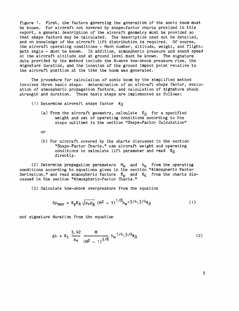
figure I. First, the factors governing the generation of the sonic boom must

be known. For aircraft not covered by shape-factor charts provided in this

report, a general description of the aircraft geometry must be provided so

that shape factors may be calculated. The description need not be detailed,

and no knowledge of the aircraft lift distribution is required. Of course,

the aircraft operating conditions - Mach number, altitude, weight, and flight-

path angle - must be known. In addition, atmospheric pressure and sound speed

at the aircraft altitude and at ground level must be known. The signature

data provided by the method include the N-wave bow-shock pressure rise, the

signature duration, and the location of the ground impact point relative to

the aircraft position at the time the boom was generated.

The procedure for calculation of sonic boom by the simplified method

involves three basic steps: determination of an aircraft shape factor, evalu-

ation of atmospheric propagation factors, and calculation of signature shock

strength and duration. These basic steps are implemented as follows:

(I) Determine aircraft shape factor KS

(a) From the aircraft geometry, calculate KS for a specified

weight and set of operating conditions according to the

steps outlined in the section "Shape-Factor Calculation"

or

(b) For aircraft covered by the charts discussed in the section

"Shape-Factor Charts," use aircraft weight and operating

conditions to calculate lift parameter and read KS

directly.

(2) Determine propagation parameters Me and he from the operating

conditions according to equations given in the section "Atmospheric Factor

Derivation," and read atmospheric factors Kp and Kt from the charts dis-cussed in the section "Atmospheric-Factor Charts."

(3) Calculate bow-shock overpressure from the equation

APma x = KpKR p_-_vPg (M2 - 1)1/8he-3/4Z3/4Ks (i)

and signature duration from the equation

3.42 M

At = Kt

av (M2 - I)3/8

hel/4z3/4K S (2)

SHAPE-FACTORCALCULATION

The computer method of reference 6 has been considerably simplified toobtain the following procedure for calculation of aircraft shape factor fromgeometric data.

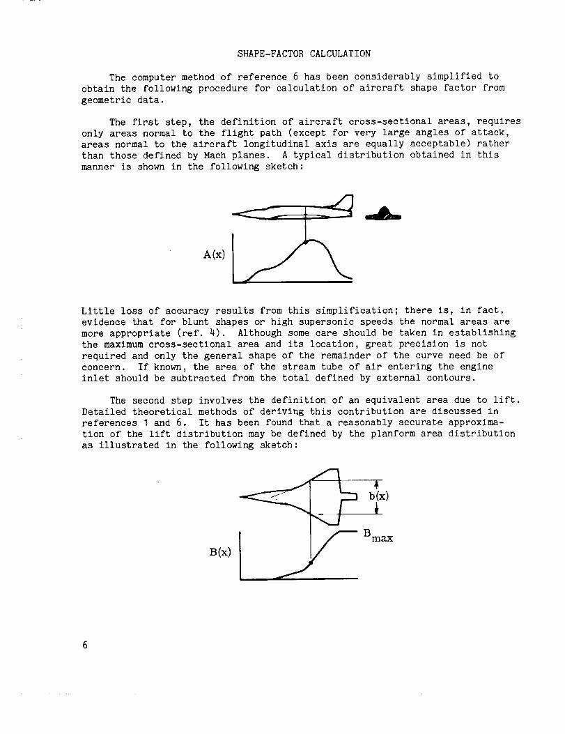
The first step, the definition of aircraft cross-sectional areas, requiresonly areas normal to the flight path (except for very large angles of attack,areas normal to the aircraft longitudinal axis are equally acceptable) ratherthan those defined by Machplanes. A typical distribution obtained in thismanner is shownin the following sketch:

A(x)

Little loss of accuracy results from this simplification; there is, in fact,evidence that for blunt shapes or high supersonic speeds the normal areas aremore appropriate (ref. 4). Although somecare should be taken in establishingthe maximumcross-sectional area and its location, great precision is notrequired and only the general shape of the remainder of the curve need be ofconcern. If known, the area of the stream tube of air entering the engineinlet should be subtracted from the total defined by external contours.

The second step involves the definition of an equivalent area due to lift.Detailed theoretical methods of deriving this contribution are discussed inreferences I and 6. It has been found that a reasonably accurate approxima-tion of the lift distribution may be defined by the planform area distributionas illustrated in the following sketch:

B(x)S Bmax

6

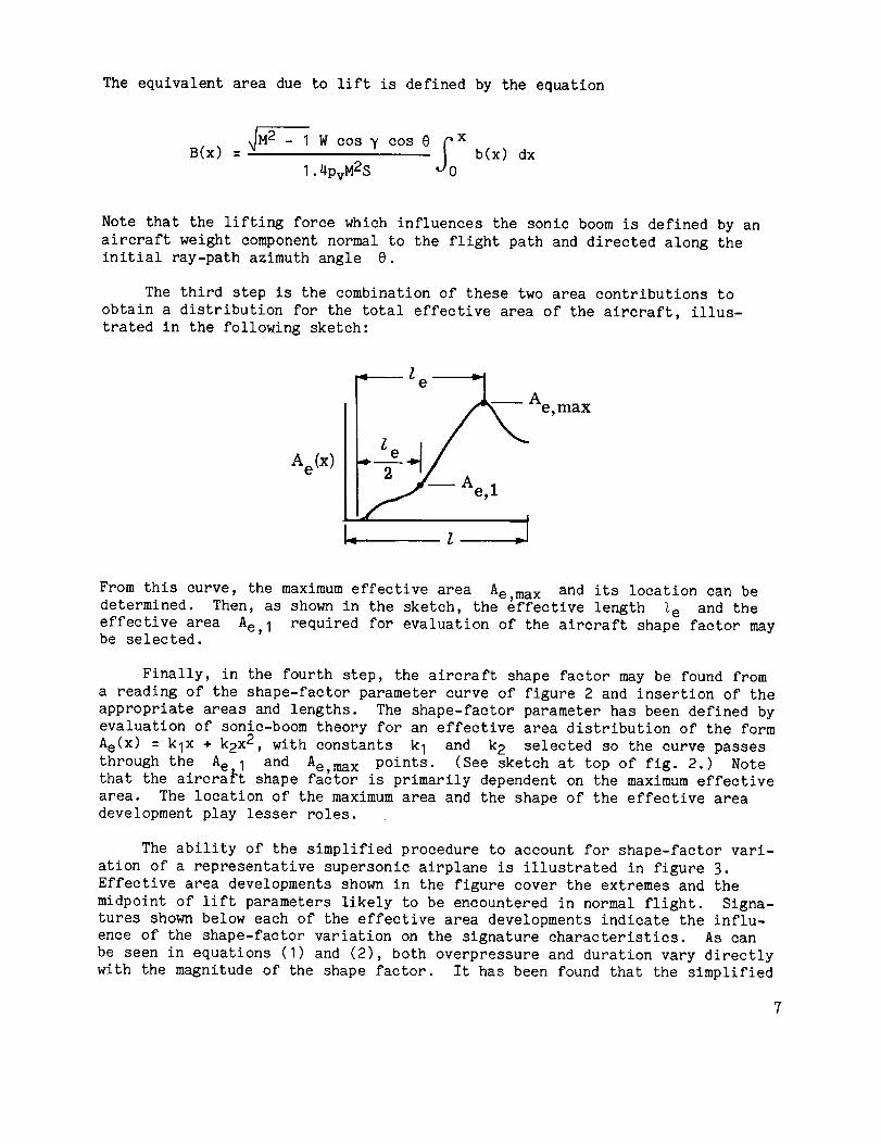
The equivalent area due to lift is defined by the equation

M2 - I W cos _ cos 8_ xB(x) : b(x) dx

Jo1.4PvM2S

Note that the lifting force which influences the sonic boom is defined by an

aircraft weight component normal to the flight path and directed along theinitial ray-path azimuth angle e.

The third step is the combination of these two area contributions to

obtain a distribution for the total effective area of the aircraft, illus-trated in the following sketch:

Ae (x)

_____ Ze _,

Ae, max

_/-- Ae, 1

From this curve, the maximum effective area Ae max and its location can be

determlned. Then, as shown in the sketch, the effective length Ze and the

effective area Ae, I required for evaluation of the aircraft shape factor maybe selected.

Finally, in the fourth step, the aircraft shape factor may be found from

a reading of the shape-factor parameter curve of figure 2 and insertion of the

appropriate areas and lengths. The shape-factor parameter has been defined byevaluation of sonic-boom theory for an effective area distribution of the form

Ae(X) = klX + k2x2 , with constants k I and k2 selected so the curve passes

through the Ae I and Ae,ma x points. (See sketch at top of fig. 2.) Notethat the aircraft shape factor is primarily dependent on the maximum effective

area. The location of the maximum area and the shape of the effective area

development play lesser roles.

The ability of the simplified procedure to account for shape-factor vari-

ation of a representative supersonic airplane is illustrated in figure 3.

Effective area developments shown in the figure cover the extremes and the

midpoint of lift parameters likely to be encountered in normal flight. Signa-tures shown below each of the effective area developments indicate the influ-

ence of the shape-factor variation on the signature characteristics. As can

be seen in equations (I) and (2), both overpressure and duration vary directly

with the magnitude of the shape factor. It has been found that the simplified

curve-fit method gives shape factors which are generally within 5 percent (andalmost always within 10 percent) of the values given by the more rigorous theo-retically based computer methods.

SHAPE-FACTORCHARTS

For the reader's convenience, aircraft shape factors for a variety of air-planes employed in sonic-boom flight-test programs and for more contemporaryaircraft are given in the charts of figure 4. To use these charts it is nec-essary only to identify the aircraft of concern, calculate the lift parameterKL, and readthe shape factor directly. Note that with the exception of thespace shuttle orbiter, which is set apart as a result of its high volume, shapefactors for all the aircraft fall in a fairly narrow band. For aircraft notspecifically covered by the charts, shape factors may be chosen by selectinga similar configuration. Generally, larger airplanes are more slender and willhave lower shape factors. Fighter airplanes, on the other hand, tend to havehigher shape factors. At the upper end of the lift-parameter range, the shapefactor is more dependent on the wing planform than on the aircraft size andvolume, and highly swept wings tend to have better shape factors.

There is no great sensitivity of the final overpressure and duration cal-culations to the choice of the aircraft characteristic length _, even thoughit appears as a squared term in the lift parameter. It is important, however,that the chosen length be used consistently throughout the calculations.

If, as mentioned in the introduction, it becomesnecessary to considerthe effects of curved flight paths and acceleration in situations where far-field conditions are to be expected, the shape factor provided by this simpli-fied prediction method maybe used to supply an input F-function for the atmo-spheric propagation program of reference 5. The necessary F-function mayberepresented by a double triangular distribution as shownin the followingsketch:

F-function

z Jr!

-3.46Ks2 _

8

Definition of the lifting force normal to the flight path used in shape-factor

determination must now include the effects of aircraft accelerations; it is no

longer appropriate to use only a component of the aircraft weight as is done

throughout this report.

ATMOSPHERIC-FACTOR DERIVATION

Atmospheric propagation factors for ray-path distance, pressure amplifica-

tion, and signature duration have been derived from repeated use of the sonic-

boom propagation computer program described in reference 5 for a matrix of

altitudes, Mach numbers, ray-path azimuth angles, and flight-path angles. To

determine these factors, the program was run first with a standard atmosphere,

and then with a uniform atmosphere with a pressure equal to the geometric mean

of the standard atmospheric pressures of the aircraft altitude and at ground

level, P_-PvPg. The factors are simply the ratios of sonic-boom parametersgiven by the first run to those given by the second.

In order to broaden the applicability of the atmospheric propagation

factors and allow the use of on-track and level-flight data for off-track and

flight-path-angle conditions, the concepts of effective Mach number and effec-

tive altitude were employed. It was presumed that the ray-path curvature and

the overpressure amplification due to atmospheric effects would depend primar-

ily on the initial inclination of the aircraft-generated ray path with respect

to the earth plane and on the ray-path distance measured perpendicular to the

aircraft flight path. A convenient measure of the ray-path inclination is the

Mach number for level flight, which would have the same ray-path angle in the

flight-track plane. This is termed the effective Mach number. The ray-path

distance measured perpendicular to the aircraft flight path is termed the

effective altitude. Geometric relationships used in the derivation of these

parameters are illustrated in figure 5. Simplified equations for effective

Mach number, propagation distance, and effective altitude for the on-track

case are as follows:

M e = (3)

sin (y + cot -I_ - I)

(Kd from fig. 7(b)) (4)

h e : h cos y + dx sin y (5)

Complete equations for the more general off-track case are as follows:

Me -

1 +

(tan 7 +

c I ( tan Y )] 2I

tan e )]2_ (tan2 7 + I+

(6)

(h)d : Kd

QMe 2- I

(7)

tan @ cos y (I + tan 2 y)= tan -I (8)

1tan y +

cos 0 _ - I

dx : d cos _ (9)

dy : d sin ¢ (10)

he : _dy 2 + (h cos y + dx sin y)2 (11)

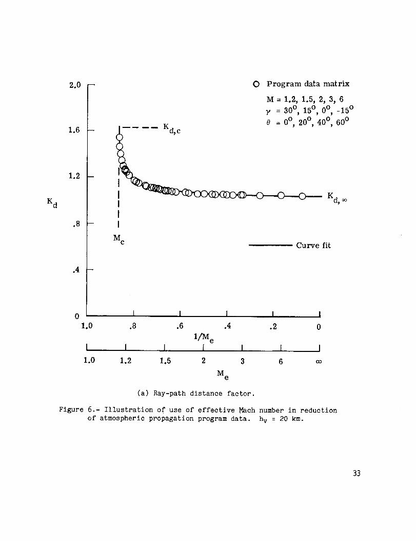
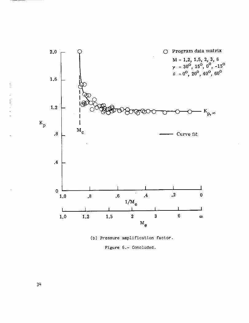
The usefulness of the effective Mach number and effective altitude in

reducing a large amount of computer-generated data to manageable proportions

is illustrated in figure 6. For a selected altitude of 20.0 km, ray-path dis-

tance factor Kd and pressure amplification factor Kp are shown as a func-tion of the effective Mach number. The Mach number scale was chosen in order

to cover Mach numbers from one to infinity with an expansion of the lower Mach

number range. Program-generated data are given for ray-path azimuth angles

from 0° to 60 ° and for flight-path angles from -15 ° to 30°. The nesting of

the data verifies the concepts of the effective Mach number and the effective

altitude. For other altitudes up to about 70 km, the tendency toward collapse

of the data to a single line is generally somewhat more pronounced than that

shown in figure 6.

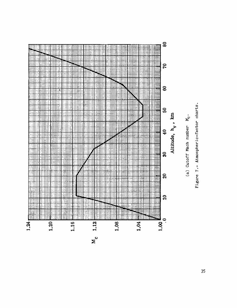
ATMOSPHERIC-FACTOR CHARTS

Atmospheric factors required in this simplified method for sonic-boom

prediction are presented in figure 7. The first chart (fig. 7(a)) gives the

cutoff Mach number in a standard atmosphere as a function of aircraft altitude.

Cutoff occurs for disturbances which propagate away from the aircraft along a

I0

ray path (as defined by the effective Machnumber) which curves under theinfluence of atmospheric gradients to an extent just sufficient for it tobecomehorizontal at ground level. As is discussed later, this cutoff limitsthe lateral extent of the ground area affected by the sonic boom. If theeffective Machnumber calculated according to the appropriate equation fromthe preceding section is not greater than the cutoff Machnumber for the alr-craft altitude, there is no need to go further; the signal will not reach theground.

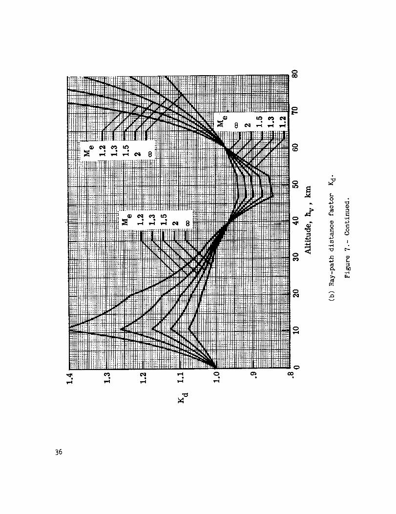
Ray-path distance factors are given in figure 7(b). The horizontaldistance traveled by a particular ray path from the time a signal leaves theaircraft until it reaches the ground maybe found by using this factor. Thefactor read from the chart for a given altitude and effective Machnumberis simply multiplied by the distance traveled in a uniform atmosphere/ -- \

(h/_Me2- 11 . Interpolation must be done with care because of the nonlinear

nature of the data. There is no need to use the ray-path distance-factor

charts for estimates of level-flight on-track overpressure; they are required,

however, to obtain an effective altitude for overpressure calculation at off-

track locations and for flight-path angles other than zero.

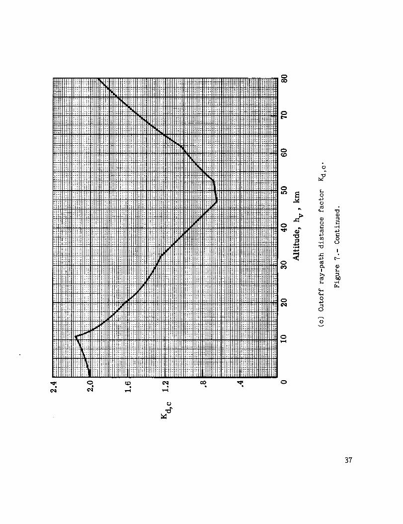
The limiting or cutoff ray-path distance factor may be read from fig-

ure 7(c). The primary use of this chart is in defining the lateral extent

dy,c of the affected ground area for level flight given by

h IMc22 - Mr2dy'c = Kd'c _ - I

The chart is also useful in defining the sonic-boom footprint limits for mod-

erate climbing or descending flight profiles. These limits, however, must be

found by iteration. The cutoff distance chart was prepared from an analysis

given in reference 7. The computer program of reference 5 does not provide

this information since calculations are terminated when ray paths come within2° of the horizontal.

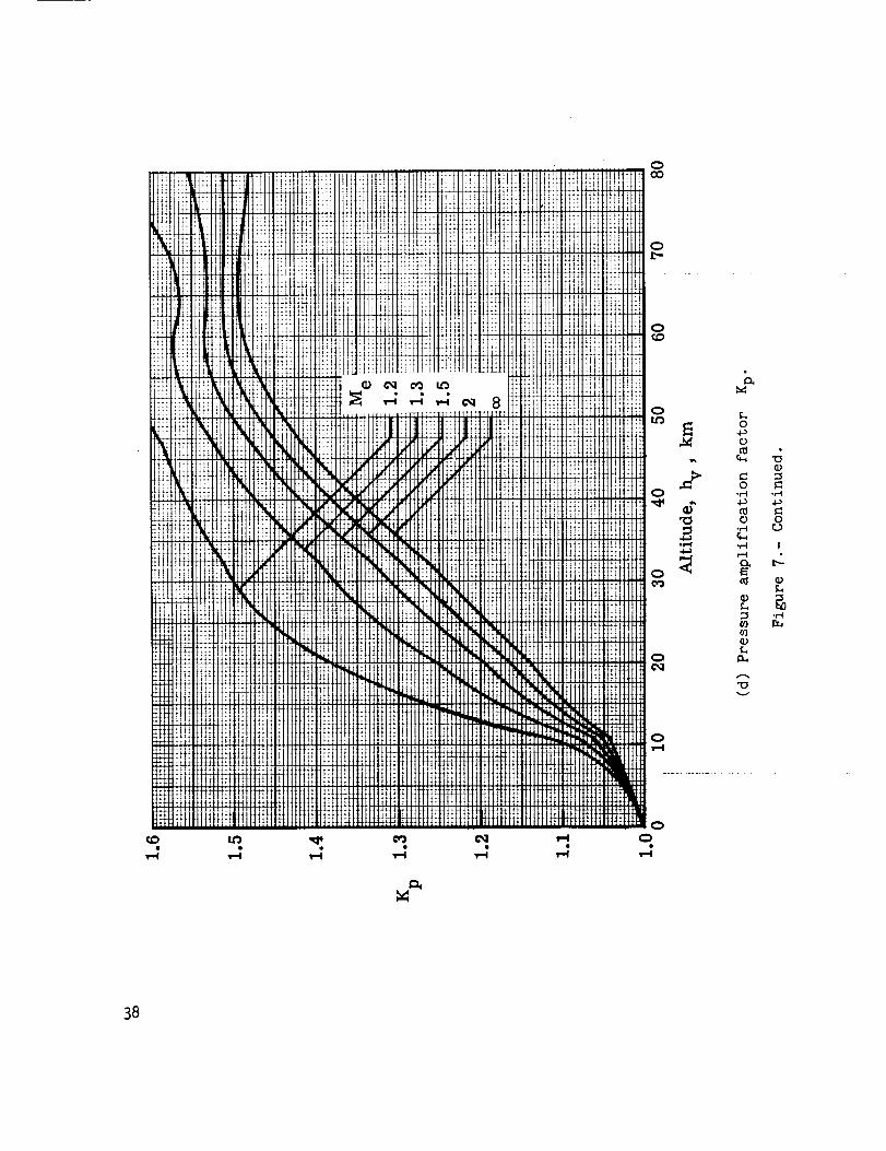
Pressure amplification factors are presented in figure 7(d). Care is

required for accurate interpolation of the charts because of the nonlinear

nature of the data. This factor, in combination with the effective-altitude

term, accounts for nonuniform atmospheric effects in the equation for bow-

shock overpressure given in equation (I).

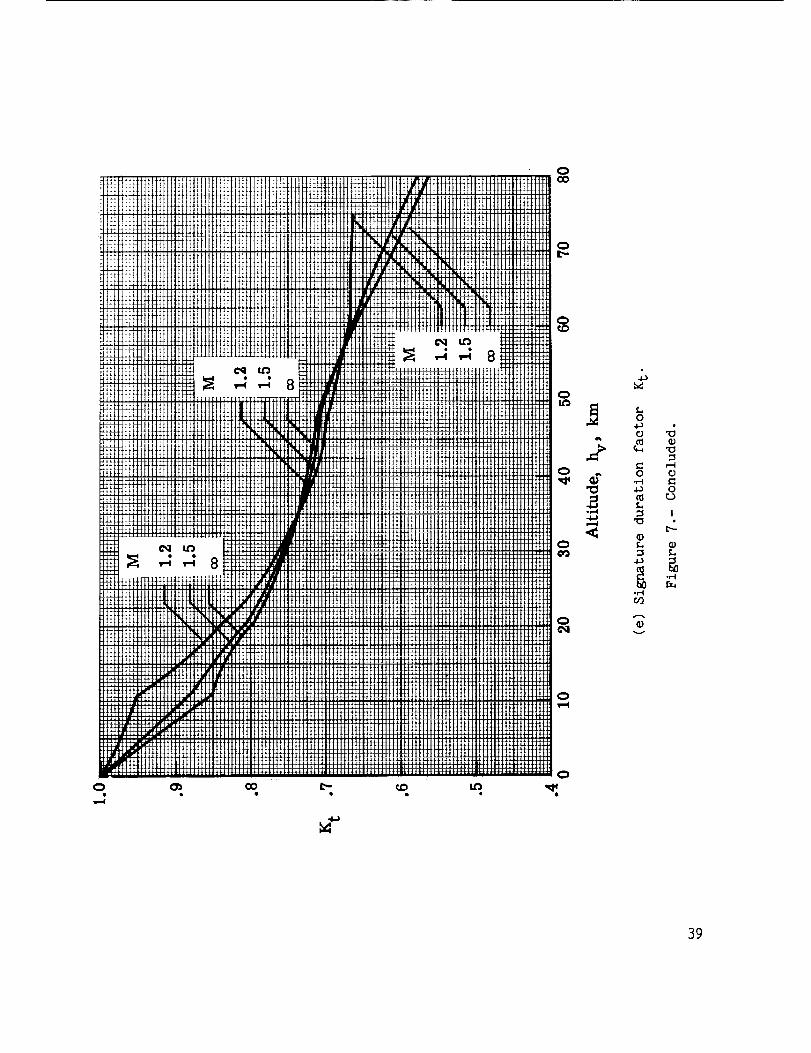
The final atmospheric-factor chart (fig. 7(e)) gives the signature dura-

tion factor which, in combination with the effective-altitude term, accounts

for the effects of a nonuniform atmosphere in the equation for signature dura-

tion given in equation (2). The actual Mach number rather than the effective

Mach number is used when reading this chart.

The atmospheric-factor charts presented herein apply directly to the sit-

uation where ground level is at or near sea level. The charts can, however,

11

be used with little error for ground levels up to about 1600meters. The air-craft altitude above sea level hv should be used when entering the charts,and the altitude above ground level h should be used when calculating theeffective altitude and propagation distances.

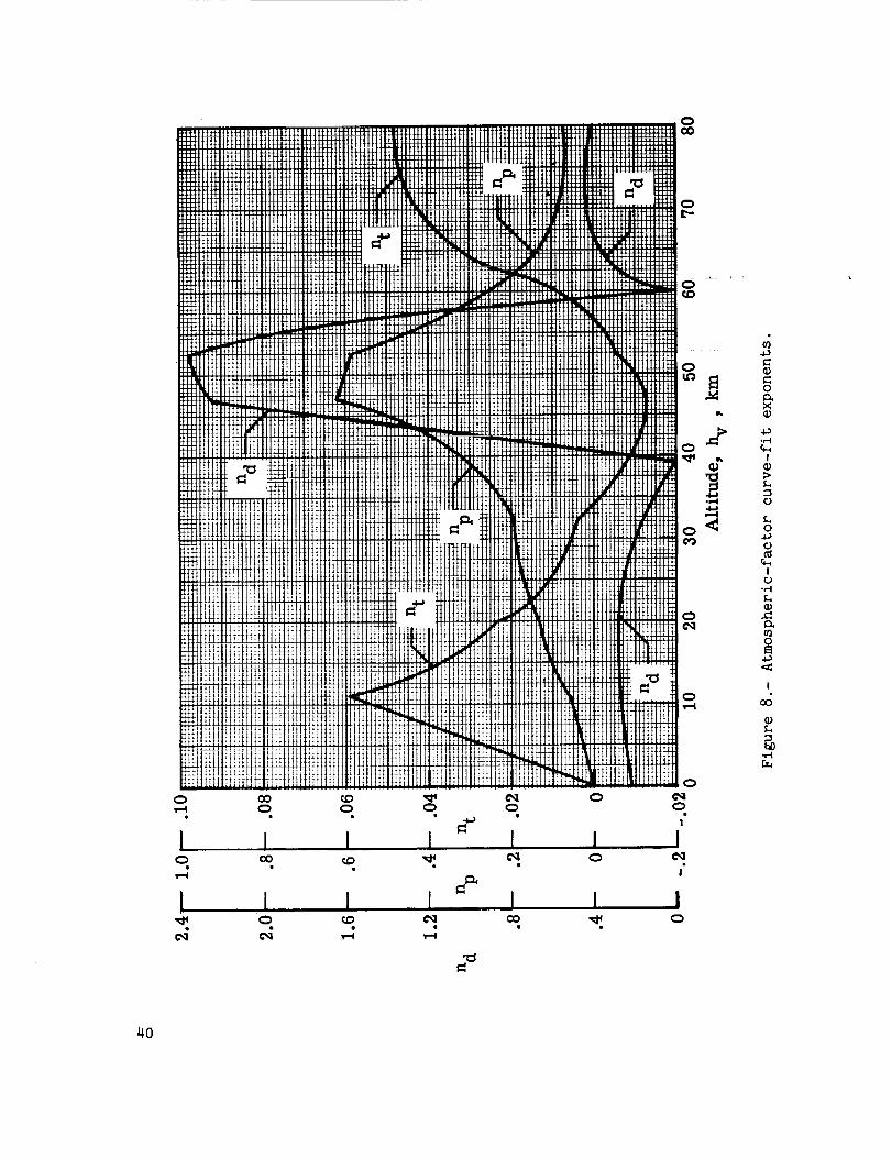
Generally, the atmospheric propagation factors maybe read directly fromthe previously discussed charts. However, the charts which cover only Machnumbersgreater than 1.2 do not give sufficient information for situations inwhich cutoff conditions are approached. To cover these situations, the follow-ing curve-fit equations which employ exponents given in figure 8 maybe used:

Me- cKd = Kd,c + (Kd,_ - Kd,c) (12)

=(1In,Kp = Kp,_o _Ic/

(13)

/ M hnt(14)

The form of these curve-fit equations was suggested by the nature of the pro-

gram data as exemplified in figure 6. The asymptotic approach of the factors

to limiting values at Mach numbers approaching infinity should be noted. The

pressure factor displays singular behavior as the cutoff Mach number is

approached, but the distance factor has a finite limit at this Mach number.

These characteristics were taken into account in the formulation of the curve

fit. An example of the curve-fit approximation is given in figure 6.

Equations (12) to (14) and the exponent curves of figure 8 appear to be

somewhat formidable. The information, however, may be employed in a rather

straightforward manner. First, it is necessary to define the cutoff Mach num-

ber and limiting values of the atmospheric factors from figure 7. Then, for

the given altitude, read the curve-fit exponents for each of the three factors

from the chart of figure 8. Finally, find the atmospheric factors by substi-

tuting the desired effective Mach number, the cutoff Mach number, the limiting

factors, and the curve-fit exponents into equations (12) to (14).

SIGNATURE CALCULATION

In the preceding sections, means of obtaining an aircraft shape factor

were described and the procedure for reading atmospheric propagation factors

from the charts was outlined. In the process of evaluating the atmospheric

propagation factor, the location of the impact point on the ground relative to

12

the position of the aircraft at the time of generation (dx and dy) is alsoprovided.

With the shape factors and atmospheric factors in hand, the signature may

be calculated by applying equations (I) and (2). All the terms are described

in the section "Symbols" and some are discussed in detail elsewhere in this

report.

It may be of help here to discuss the reflection factor KR. When the

shock wave meets the Earth, flow velocities behind the shock are altered;

vertical velocities are blocked and their energy is converted into a pressure

increase. For weak shocks meeting a smooth, rigid, and flat surface, the

resultant overpressure is theoretically twice that of the free-air value ofthe incident wave. In flight tests, reflection factors varying from about 1.8

to 2.0 have been recorded. The lower values are generally associated with

sandy or marshy terrain. For ground overpressure predictions presented in

this report, a reflection factor of 2.0 has been assumed.

Although the calculative procedures are relatively straightforward andsimple, it may be desirable to utilize the programming capabilities of some of

the modern pocket-sized or desk-top calculators for repetitive calculations.

Some notes on programming are offered in appendix A.

A series of three sample problems has been prepared to aid the reader in

understanding the calculation process. These problems are presented in

appendix B.

CORRELATION WITH FLIGHT-TEST DATA

To demonstrate the applicability of the simplified sonic-boom prediction

method to a variety of problems, correlations with flight-test data (refs. 8

to 14) are shown in figures 9 to 13.

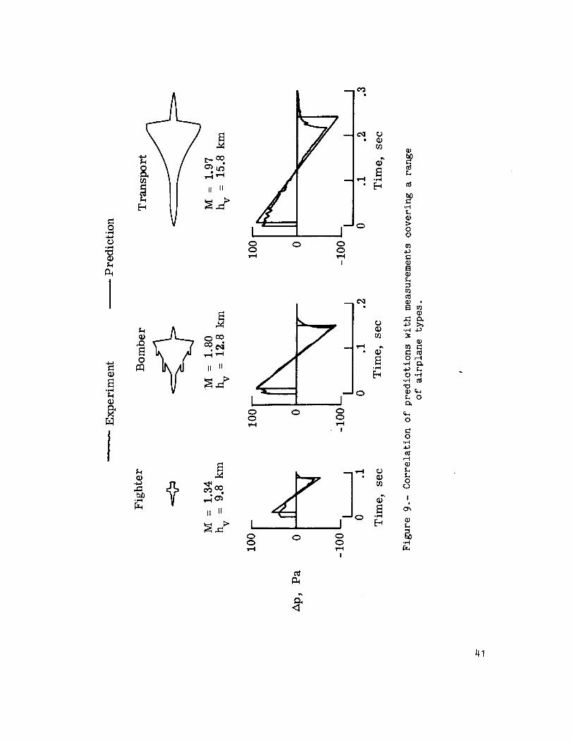
In figure 9, predictions are compared with measured signatures for threedistinct airplane types (refs. 8 and 9) operating at or near cruise conditions.

Only for the fighter aircraft, which displays some evidence of near-fieldeffects, is there an appreciable difference between predicted and experi-

mental results. In this situation, as noted previously, the prediction isconservative.

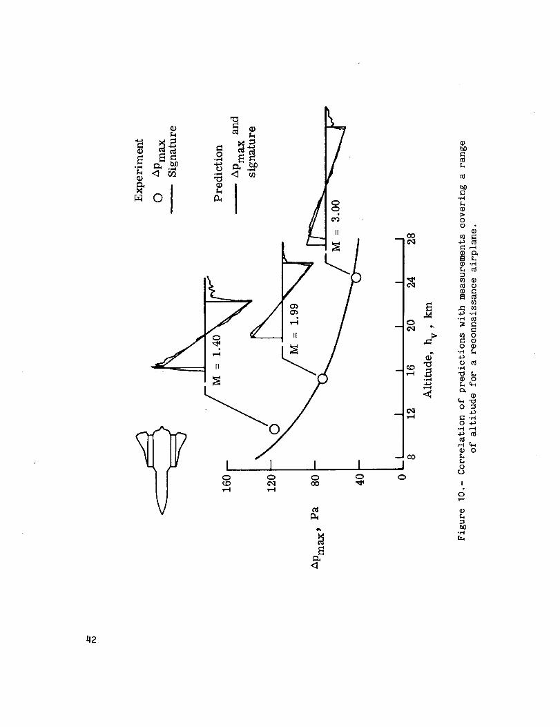
Correlations of predictions with measurements for a reconnaissance air-

plane (ref. 10) covering a range of flight altitudes are shown in figure 10.

The variation of Apma x with hv is quite typical of that for most airplanes;the Mach number differences are of secondary importance.

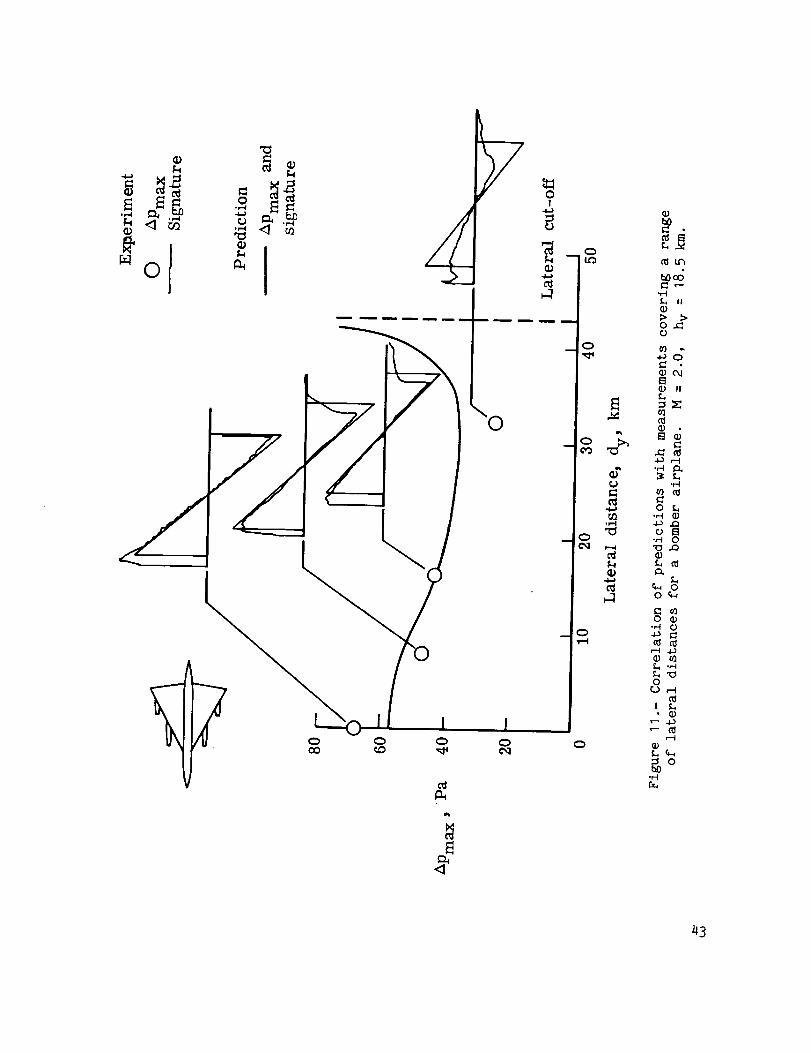
The validity of the method for off-track predictions for a bomber air-

plane (ref. 8) is illustrated in figure 11. At large lateral distances, theray paths curve sufficiently to approach the Earth at near-grazing angles.

This results in signature distortions and ultimately in a breakup of a recog-

nizable signature into random noise beyond the lateral cutoff. Therels some

evidence of such a transition for the moat distant signature shown in the

13

figure. In general, the variations with lateral distance are predicted reason-

ably well; however, there is a singularity predicted at the cutoff point which

does not appear to materialize. Other examples of measured lateral-spread

patterns are given in reference 15. No evidence of pressure amplification at

the cutoff point is shown in reference 15, and the authors apparently have

chosen to fair the prediction curve in a monotonically decreasing fashion

rather than attempt to define the theoretical singularity. Users of this

system may choose to do likewise.

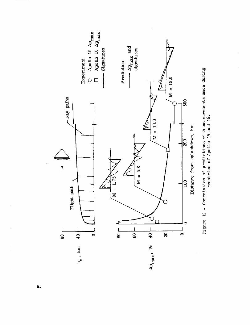
It is remarkable that the predictions for the Apollo command modules

shown in figure 12 bear any similarity to the measured data (refs. 11 and 12).

The diameter-length ratio of the effective body shape is about 9 and the

effective length is only 0.42 m. The appearance of the unexpected multiple

shocks in the measured signatures remains unexplained. Although the correla-

tions are far from exact, the predictions are nevertheless useful. Especially

notable is the degree of correlation indicated for a Mach number of 15.

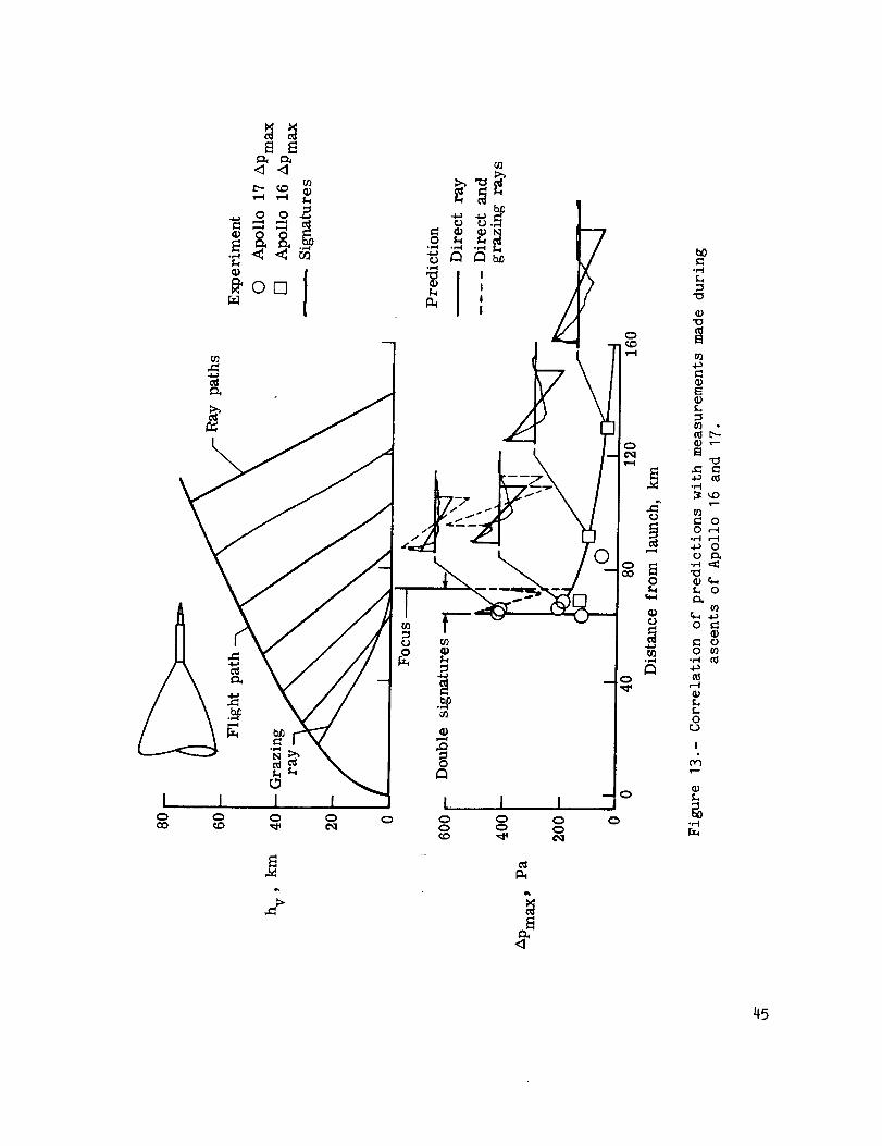
Another example of the applicability of the simplified prediction method

to spacecraft is given in figure 13. As mentioned in the discussion of the

sample problems (appendix B), the sonic boom generated by the Apollo launch

vehicles (refs. 12 and 13) is dominated by the exhaust gas plume, so this is

a very special situation. Another special feature is the ground pattern of

the signatures. As shown in the flight-path profile there are two families

of rays. One family consists of near-grazing rays generated prior to genera-

tion of that ray which reaches a point nearest the launch. The other family

consists of more direct rays generated after that time. As can be seen on

the plot of overpressure versus distance from launch, there is a portion of

the ground track over which double or superimposed signatures are predicted.

It is apparent from the inset pressure-signature sketches that the grazing-

ray component of these signatures is grossly overpredicted. However, the

pressure-doubling at the closest ground intersection point appears to have

materialized. Large distances traveled in proximity to the Earth appear to

cause disintegration of a distinct signature into random noise. There is

also a question as to whether grazing rays should be considered to have a sur-

face reflection factor of 2 or a free-air reflection factor of I. These data

seem to indicate that the grazing-ray pressure signatures should be ignored.

However, at the first ground-track point, members of the grazing-ray family

have not yet reached grazing conditions and thus contribute to the signature.

With this stipulation, the predicted overpressure indicated by the solid line

agrees reasonably well with the measured data. The predicted signature dura-

tion, however, as indicated by the sketches, is too large by a factor of

nearly 2. The curved flight path and the vehicle acceleration may play some

part in the cause of the discrepancy.

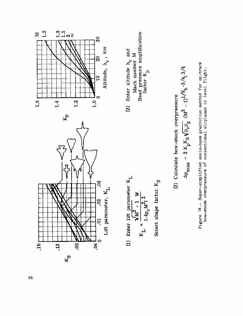
FURTHER SIMPLIFICATION

For readers interested only in prediction of on-track overpressure for

conventional airplane configurations, several of the steps in the general

simplified method may be omitted. In this case it is possible to place all

the necessary information, with the exception of atmospheric tables, on a

single page. This "super simplified" method is given in figure 14.

14

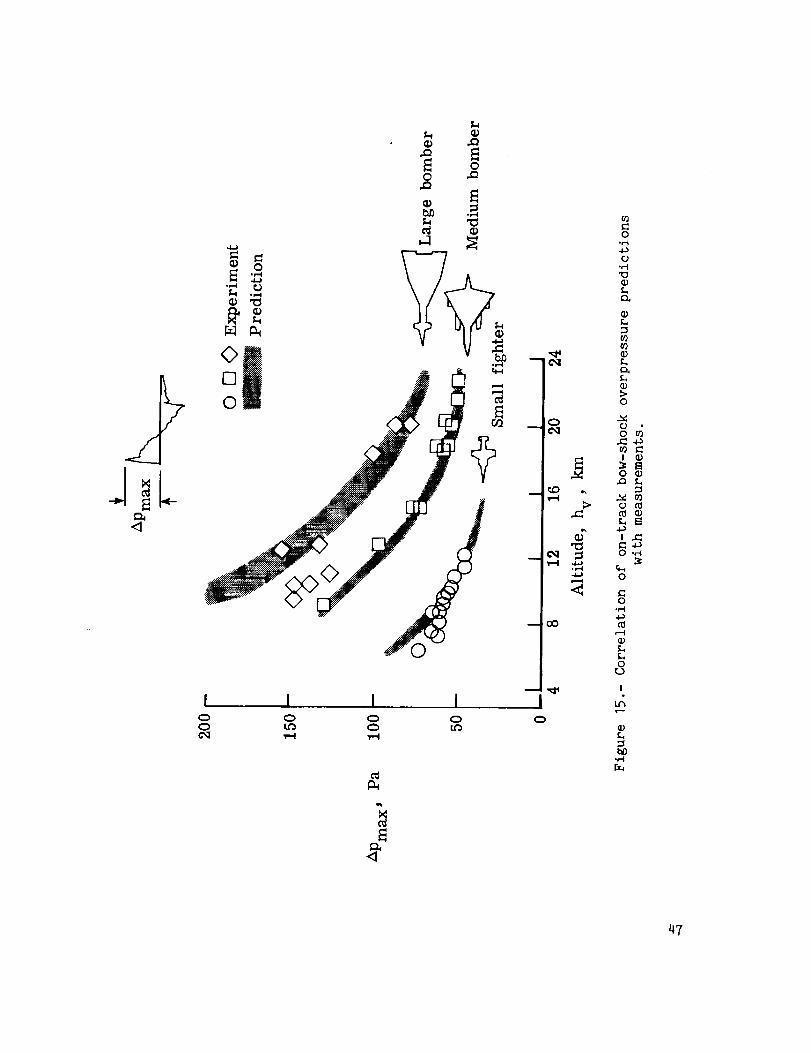
Predictions obtained by this method are compared with flight-test data for

three airplanes (refs. 8 and 14) in figure 15. Each prediction is shown as a

band to account for variations in airplane weight and Mach number that occur

at a given altitude. Deviations of predictions from measurements occur at the

lower altitudes for both the large bomber and the small fighter. These dif-

ferences arise because the simplified methods do not account for the presence

of a small amount of near-field effect in the signatures generated by these

airplanes. Such discrepancies are anticipated for very large and slender air-

planes, but the measured signatures for the small fighter are not at all typi-cal of fighter aircraft. The near-field effect for the fighter is due to the

nontypical long slender nose. A redeeming quality of the prediction method

is that when near-field effects do occur, the prediction tends to beconservative.

CONCLUDING REMARKS

A simplified method for calculation of the sonic-boom characteristics of

greatest interest for a wide variety of airplane configurations and spacecraft

has been described. The procedure, which has been outlined in a step-by-step

manner, relies to a great extent on the use of charts to provide the necessarysonic-boom generation and propagation factors for use in relatively simple

expressions for signature characteristics. Computational requirements can be

met by hand-held scientific calculators or by slide rules. With little sacri-

fice in accuracy, complete calculations can often be obtained in less time

than is required for the preparation of computer input data for the more

rigorous calculation methods. A variety of correlations of predicted and

measured sonic-boom data for airplanes and spacecraft serve to demonstrate

the applicability of the method.

Langley Research Center

National Aeronautics and Space AdministrationHampton, VA 23665

January 31, 1978

15

APPENDIX

NOTESONPROGRAMMING

As was mentioned in the main body of the report, it was found that thecomputational needs of the simplified sonlc-boom prediction method could bemet by hand-held scientific calculators. With programmablepocket-sized ordesk-top calculators, the labor of performing the calculations can be reducedto an almost negligible level. Somenotes on strategy for employmentof pro-grammablecalculators are offered here.

Before a programmedsolution may be employed, it is necessary to haveshape-factor charts for the aircraft of concern. For aircraft not covered infigure 4, a shape-factor chart maybe prepared according to the steps outlinedin the section "Shape-Factor Calculation."

It was found to be convenient to calculate the atmospheric factors first.The primary input quantities are the flight conditions M, e, y, and hvand the ground level hg. If the curve-fit data are to be used in determina-tion of the atmospheric factors, the quantities Mc, Kd =, Kd c, K, _,Kt _, nd, nn, and nt read from the charts for the fl_g_ht al_itude_a_y alsobe'_sed as initial input.

The effective Mach number Me and the ray-path azimuth angle ¢ may becalculated as follows:

Me=It +

[A(I - B tan y)]2

[A(tan y + B_2 + (CD)2

where

: °)\ tan y + A

A -

B -

C -

rocos y gM _ - I

I

cos e_M _ - I

tan @

_"M2 _ 1

D = tan 2 y + I

16

APPENDIX A

With the effective Mach number known, the atmospheric factors may be determined

either from a direct reading of the charts (which requires a program temporary

stop for chart reading and input of Kd, Kp, and Kt) or from the curve-fitdata. When evaluating atmospheric factors from the curve-fit data, first test

Me to see if it is greater than M c. If it is not, the calculation must be

terminated; the ray path chosen will not reach the ground. To evaluate the

atmospheric factors Kd, Kp, and Kt from the curve-fit data, use the follow-ing expressions:

Me - c

Kd = Kd, c + (Kd - Kd,_ ,c ) Me

Kp : Kp'_ Mc

I M Int

The ground location of the boom and the effective altitude may now befound as follows:

Kd(h v - hg)d =

2 - I

dx : d cos ¢

dy = d sin

he = _dy 2 + [(h v - hg) cos y + dx sin y]2

To calculate the magnitude of the sonic-boom overpressure, first evaluate

the lift parameter KL as follows:

KL :_- I W cos y cos 0

1.4PvM2_2

When KL is known, it is necessary to provide another temporary stop for

reading and input of the aircraft shape factor from the appropriate curve. In

17

APPENDIXA

addition, the quantities Pv, Pg, av, and KR must be input. Nowthe bow-shock overpressure and the signa£ure duration maybe calculated as follows:

Apmax = KpKRP_vPg(M2 - 1)I/8he-3/4%3/4KS

3.42 MAt = Kt -- hel/4z3/4Ks

av (M2 - i) 3/8

Any consistent set of measurementunits maybe used as input. The over-pressure will be in the units of the atmospheric pressure and the signatureduration will be in the time unit used for the speed of sound.

18

APPENDIX B

SAMPLE PROBLEMS

The calculations required for the three sample problems are presented in

this appendix with only a brief explanation. The first sample problem illus-

trates the calculation of the shape factor from aircraft geometric data, in

this case taken from small-scale three-view drawings such as those found in

reference 16. The calculations shown in the second problem cover the situa-

tion in which an aircraft shape factor may be read from the charts. The off-

track signature calculation, however, is somewhat more complicated than the

on-track calculation of the first sample problem. The third problem covers

an unusual situation in which the sonic-boom behavior is dominated by the

exhaust gas plume of the propulsion system rather than by the vehicle itself.

This problem also demonstrates the versatility of the simplified method. The

area of the exhaust gas plume of the ascending Apollo launch vehicle was

obtained from data presented in reference 17.

Sample Problem I: Reconnaissance Airplanes, On-Track

The flight conditions and geometric data are

M= 1.99 W : 41 000 kgf : 402 000 N

I : 32.7 m y : 0o 0 : 0o

hv : 15.240 km Pv = 11.6 kPa av = 295 m/sec

hg = 0.760 km pg = 92.3 kPa KR : 2.0

h = hv - hg = 14.480 km

The aircraft shape factor is obtained as follows:

2-IW_x= =I0-7m2

1.4PvM2

19

From the area plots at right(from data given in ref. 16)

_e:24m

15.0 m2Ae,max =

Ae,I = 4.4 m2

Ae,I/Ae,max = 0.29

From figure 2,

A_e _max

KS = 0.685 = 0.087Z3/4 ZI/4

APPENDIX B

J

/-3

B

Bm_ix '°I.50

I_ l e -

16 - le _1_,_e,max

Ae, m 2 81/_/__ Bmax

0

Propagation factors are obtained from equations (3) to (5) and figure 7.

Me =M: 1.99

h e : h : 14.480 km

Kp : 1.10

Kt : 0.85

The signature is calculated as follows:

APma x = KpKR Pv_ (M2 - 1)1/8he-3/4Z3/4Ks = 74 Pa

3.42 M

At : Kt_av (M2 - i)3/8

hel/4z3/4K S : 0.17 sec

2O

APPENDIXB

SampleProblem 2: MediumBomberAirplane, Off-Track

The flight conditions and geometric data are

M=2.0 W = 36 000 kgf = 353 000 N

: 30 m y : 0° O : 52°

hv = 18.600 km Pv = 6.88 kPa av = 296 m/sec

hg = 0.760 km pg = 92.3 kPa KR : 2.0

h = hv - hg = 17.840 km

The aircraft shape factor is obtained from figure 4.

M2 - I W cos y cos eK L = = 0.0108

1.4PvM2Z2

KS : 0.088

Propagation factors are obtained from equations (6) to (14) and

figures 7 and 8.

M e : 11 +

cos 2 e (M2 - I)

I + cos 2 e tan 2 e (M2 - I)

= 1.182

d = Kd = 37.4 km

Me2 - I

¢ = tan -I (tan e cos e_- I)= 53.8 °

dy = d sin ¢ = 30.2 km

he = _dy 2 + h2 = 35.1 km

21

APPENDIXB

Mc : 1.153

Me - cKd = (Kd,_ - Kd,c) + Kd,c = 1.32

MI_- I InPKp = Kp _ -- 1.42' Mc

/ M _ nt

Kt = Kt,_l_- q_ : 0.82

The signature is calculated as follows:

APmax = KpKR P_-_vP_ (M2 - 1)1/8he-3/4Z3/4K S = 36.1Pa

3.42 MAt = Kt

av (M2 - i)3/8

hel/413/4Ks = 0.19 sec

22

APPENDIXB

SampleProblem 3: Apollo Launch Vehicle in Ascent

The flight conditions and geometric data are

M= 4.08 125 sec and 32.9 km from launch

= 104.5 m y = 31.6° 0 = 0O

hv = h = 36.1 km Pv = 0.490 kPa av : 310 m/sec

hg = 0 pg = 101 kPa KR = 2.0

The aircraft shape factor is deter-mined from area plot at right (from datagiven in ref. 17).

%e= 160 m

Ae,max : 14.7 x 103 m2

Ae,I : 5.8 x 103 m2

Ae,I/Ae,max = 0.39

From figure 2,

15-

10-

5-

0

ii

_------- l e------_ / / A/-- e,max

l

--Ae, l

KS = 0.65

Z314Ze1/4

: O.68

23

APPENDIX B

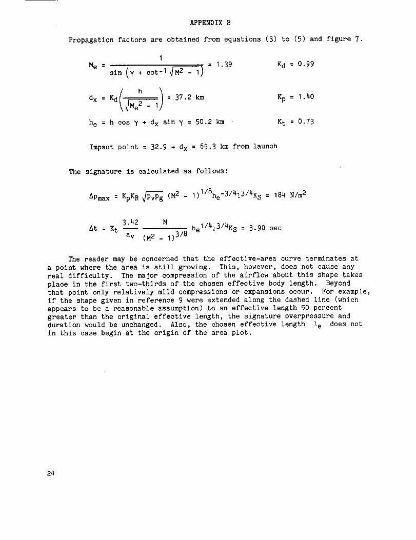
Propagation factors are obtained from equations (3) to (5) and figure 7.

M e : : 1.39 Kd : 0.99

sin (y + cot -I qM 2 - I)

(h>dx : Kd : 37.2 km

_Me 2 - I

Kp = 1.40

h e : h cos y + dx sin y : 50.2 km Kt = 0.73

Impact point = 32.9 + dx = 69.3 km from launch

The signature is calculated as follows:

APmax : KpK R _ (M2 - 1)1/8he-3/4Z3/4Ks : 184 N/m 2

3.42 MAt : K t

av (M2 - I)3/8

hel/4z3/4Ks : 3.90 sec

The reader may be concerned that the effective-area curve terminates at

a point where the area is still growing. This, however, does not cause any

real difficulty. The major compression of the airflow about this shape takes

place in the first two-thirds of the chosen effective body length. Beyond

that point only relatively mild compressions or expansions occur. For example,

if the shape given in reference 9 were extended along the dashed line (which

appears to be a reasonable assumption) to an effective length 50 percent

greater than the original effective length, the signature overpressure and

duration would be unchanged. Also, the chosen effective length Ze does not

in this case begin at the origin of the area plot.

24

REFERENCES

I. Carlson, H. W.; and Maglieri, D. J.: Review of Sonic-BoomGenerationTheory and Prediction Methods. J. Acoust. Soc. America, vol. 51,no. 2, pt. 3, Feb. 1972, pp. 675-685.

2. Hayes, Wallace D.; and Runyan, Harry L., Jr.: Sonic-BoomPropagationThrough a Stratified Atmosphere. J. Acoust. Soc. America, vol. 51,no. 2, pt. 3, Feb. 1972, pp. 695-701.

3. Holloway, Paul F.; Wilhold, Gilbert A.; Jones, Jess H.; Garcia, Frank, Jr.;and Hicks, RaymondM.: Shuttle Sonic Boom- Technology and Predictions.AIAA Paper No. 73-1039, Oct. 1973.

4. Carlson, Harry W.; and Mack, Robert J.: A Study of the Sonic-BoomCharac-teristics of a Blunt Body at a MachNumberof 4.14. NASATP-I015, 1977.

5. Hayes, Wallace D.; Haefeli, Rudolph C.; and Kulsrud, H. E.: Sonic BoomPropagation in a Stratified Atmosphere, With ComputerProgram. NASACR-1299, 1969.

6. Carlson, Harry W.: Correlation of Sonic-BoomTheory With Wind-Tunnel andFlight Measurements. NASATR R-213, 1964.

7. Kane, EdwardJ.; and Palmer, ThomasY.: Meteorological Aspects of theSonic Boom. SRDSRep. No. RD64-160(AD 610 463), FAA, Sept. 1964.

8. Hubbard, Harvey H.; Maglieri, DomenicJ.; Huckel, Vera; and Hilton,David A. (With appendix by Harry W. Carlson): GroundMeasurementsofSonic-BoomPressures for the Altitude Rangeof 10,000 to 75,000 Feet.NASATR R-198, 1964. (Supersedes NASATMX-633.)

9. Williams, M. E. L.; and Page, N. M.: Measurementof Sonic BoomFromConcorde - 002 Australia 1972. R&DRep. No. 896, Dep. Civ. Aviat.,CommonwealthAustralia, Aug. 1972.

10. Maglieri, DomenicJ.; Huckel, Vera; and Henderson, Herbert R.: Sonic-BoomMeasurementsfor SR-71 Aircraft Operating at MachNumbersto 3.0 andAltitudes to 24 384 Meters. NASATN D-6823, 1972.

11. Hilton, David A.; Henderson, Herbert R.; and McKinney, Royce: Sonic-BoomGround-Pressure MeasurementsFrom Apollo 15. NASATN D-6950, 1972.

12. Henderson, Herbert R.; and Hilton, David A.: Sonic-BoomGround PressureMeasurementsFrom the Launch and Reentry of Apollo 16. NASATN D-7606,1974.

13. Henderson, Herbert R.; and Hilton, David A.: Sonic-BoomMeasurementsinthe Focus Region During the Ascent of Apollo 17. NASATN D-7806, 1974.

25

14. Sonic BoomExperiments at EdwardsAir Force Base. NSBEO-1-67(ContractAF 49(638)-1758), CFSTI, U.S. Dep. Com., July 28, 1967.

15. Garrick, I. E.; and Maglieri, D. J.: A Summaryof Results on Sonic-BoomPressure-Signature Variations Associated With Atmospheric Conditions.NASATN D-4588, 1968.

16. Taylor, John W. R., ed.: Jane's All the World's Aircraft. McGraw-HillBook Co., c.1970.

17. Hicks, RaymondM.; and Mendoza, Joel P.: Pressure Signatures for a.00053 Scale Model of the Saturn V-Apollo Launch Vehicle With SimulatedExhaust Plumes. NASATMX-62,129, 1973.

26

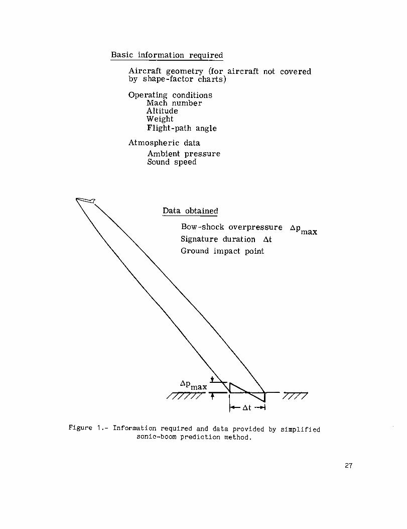
Basic information required

Aircraft geometry (for aircraft not coveredby shape-factor charts)

Operating conditionsMach numberAltitudeWeight

Flight-path angle

Atmospheric data

Ambient pressureSound speed

Data obtained

Bow-shock overpressure APmax

Signature duration At

Ground impact point

Figure I.- Information required and data provided by simplified

sonic-boom prediction method.

27

]-

I

//

\

GO

L0

!

!

L

q_

_J

28

29

•-_ _i _0 CO t _-

I I I _ I

//

i

0

q

e,D

//

I II L

i JI I

I IJ

I

_J

\\\'i

&\l

0 0

r_

0

o.

0

II

o

-,-i

0

I0

,r-t

0

f..,0

0

0

.,-I

I

r_

r,,.

3O

L_.C',,10

+

E"-

_O

I I I I

o _ _

cO C_1 cO _I 4C'Q T-I _ _ 0

G;"0

0

0

•0¢;

P,N

q11

0

co Q),'_

co

_., 0m ro

o I

o

31

Wave front.._-Z,

cot-lCM2e _ 1__,_ _ he_ . ,. _ \ _ "_ /-- Ray path \

• ii FIlIIIII]IIlIII_#III lllllJll_l_l /lllllllllll llll TIIII l

!_

(a) On-track.

(b) Off-track.

Figure 5.- Propagation geometric parameters.

32

K d

2,0 0 Program data matrix

1.6

1.2

.8

.4

0

M = 1.2, 1.5, 2, 3, 6

_, = 30 °, 15°, 0°, -15 °

K 8 = 0°, 20°, 40 °, 60 °

_ r d,c

i __ Kd,_

II

Mc Curve fit

I I I I I

1.0 .8 .6 .4 .2 0

I/M e

[ I I 1 I I J

1.0 1.2 1.5 2 3 6

Me

(a) Ray-path distance factor.

Figure 6.- Illustration of use of effective Mach number in reduction

of atmospheric propagation program data. hv = 20 km.

33

KP

2.0

1.6

1.2

.8

.4

0

C) Program data matrix

M = 1.2, 1.5, 2, 3, 6

7 = 300, 15°, 0°, -15°

8 =0 °, 20°, 40 °, 60°

I©

I ©

I

U c

I l [

1.0 .8 .6 .4

1/N eL I I I 1

1.0 1.2 1.5 2 3

------- Curve fit

Me

l

.2

(b) Pressure amplification factor.

Figure 6.- Concluded.

34

35

kl

36

00

0

0

O

o

o

.,o I_o

.,-I

4-_ t"-

U

0

0

Q

0 0

37

_D

,.2L_

38

39

0O0

0E-.

0e.D

0

0

0

0

0

I

0

0 0 0 0 0

I I I I I I• • |

I I I I i i*-4

.o

¢)

oI:IIxl

.,-I

ICD>L,

0

0

0

!o.el

_u

0S4._

I

d

,.-I

40

0°_.._

I

°_.,_

II 11

_00

0

@0 0o

II I1

m

t I0 0

!

I0

m 6.1

°_,..4

0

0 0

v.-,tI

0o

_d

°_ 4._

0 _

0 .H•r't _

r,-, 0

0

0°r--I

0

I

41

I I I I

<1

N}

N)

,_I

I>(:)

°.;

(1) .,-I

{Zl

_ O

O _

o_

_ O

O _

•_ ,---t

• O

Or_

!

O

_u

42

Q;

0

0

¢,)

0

I

0

\0

t_

<l

0

0

t_

0r.,I

_0

t_

t_

_ 0

0

o_0

L n

o ,.c::

_d

N

•r.t i_

o _

•r.-t 0

_u

_ 0

Cl r_0 0

_ -_

00,-t

• •

r--I0

_ 0

_3

I I I

-,--4

'0

'0

C_

C_'--

C_ 0_-I

o H•,-I 0.._0"_:

nOr,_0

(].,)-,-I

0

0 (l,)

r--t(1)

0r_

I

fll

°,-I

114

0., 0_<1 <1

L_" _0

._ 0 0 -_

o__

° I_OE3

I i I

7

I1)'tJ

4-_

_D

_- 00 ,-_

0C.) 0,

_ 0e_

o _

0 m

g.,0

r_

!

c¢3

°_

45

46

- 'S\

,, \'\X--- ,, _

.4 .4 .4

0

,=_

0 =,

m• i=,,4

)=-4

0

0

0• )=,,4

0,),=4

4-=) _c_ _O

v

b II

v

r.Q

0

o

r/l

!

N

0

0

m M!

o

4-_ _.I N)

0,4_=_

g_O ,-=4

O

OO ,H

(11 .r-I

tO@

O.,-I•_ ,=-=1Otl

.,-I"_ .,-IO

tl,-4

O OO .r-Itn .)_)

O ••,=4 l>

O O_90

• O.,-.I

O•,-I _,

13, tn

•,-I (D

! C_

• •

O

I O• O

.::r .C•=- 09

I

O

,M

¢:Z,<I

r_

@o

.,..4.,..4

I I I i0 0 0 0

#

0

.,..-4

i0

0.,'-4.._0

,._Q..)

f..,

::>0

0

! Ill_ No _

4-_

o .,--t

o

o°_4-_

o

!

g

47

l_Rel:x_t No. 2. Government Accession No. 3. Recipient's Catalog No.

NASA TP-II22

5. Report Date

March 19784, Title and Subtitle

SIMPLIFIED SONIC-BOOM PREDICTION

7. Author(s)

Harry W. Carlson

9. Performing Organization Name and Addre_

NASA Langley Research Center

Hampton, VA 23665

12. Sponsoring Agency Name and Address

National Aeronautics and Space Administration

Washington, DC 20546

6. Performing Organization Code

8. Performing Organization Report No.

L-I1794

10. Work Unit No.

743-04-31-01

1t. Contract or Grant No.

13. Type of Report and Period Covered

Technical Paper

14. Sponsoring Agency Code

15. Supplementary Notes

16. Abstract

A simplified method for the calculation of sonic-boom characteristics for

a wide variety of supersonic airplane configurations and spacecraft operating

at altitudes up to 76 km has been developed. Sonic-boom overpressures and

signature duration may be predicted for the entire affected ground area for

vehicles in level flight or in moderate climbing or descending flight paths.

The outlined procedure relies to a great extent on the use of charts to provide

generation and propagation factors for use in relatively simple expressions for

signature calculation. Computational requirements can be met by hand-held

scientific calculators, or even by slide rules. A variety of correlations of

predicted and measured sonic-boom data for airplanes and spacecraft serve to

demonstrate the applicability of the simplified method.

17. Key Words(Suggested by Authorls)}

Sonic boom

Shock-wave noise

19. Security Oaccif, (of this report]

Unclassified

20. Security Classif. (of this _ge)

Unclassified

18. Distribution Statement

Unclassified - Unlimited

21. No. of Pages

47

Subject Category 02

22. Price"

$_.5o

* For sale by the National Technical Information Service, Springfield, Virginia 22161NASA-Langley, 197B