Simple Polynomial Approach to Nonlinear Control

Mike Grimble and Pawel Majecki

Industrial Control Centre, University of Strathclydeand Industrial Systems and Control Ltd.,

Glasgow, Scotland

Nonlinear Multivariable CL System

Linear disturbance model: 1= fd dW A C−

Linear reference model: 1 fr rW A E−=

( )( ) ( )( )-ku t z u tΛ=W WNonlinear plant model:

Pc

Wr

Wd

r e u + -

y

d

W + +

m

Fc Disturbance model

Control weighting

Reference

Error weighting

+ + ξ

C0

Nonlinear plant Controller

0 c cP e uφ = + F

ω

Diagonal matrix of delays

Advantage of NGMV is only knowledge of NL plant model required is ability to compute an output for a given control input sequence.

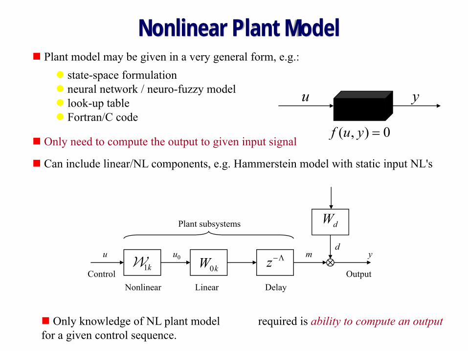
Plant model may be given in a very general form, e.g.:state-space formulationneural network / neuro-fuzzy modellook-up tableFortran/C code

Nonlinear Plant Model

Can include linear/NL components, e.g. Hammerstein model with static input NL's

( , ) 0f u y =Only need to compute the output to given input signal

1kW 0kW z−Λ

dW

ControlNonlinear Linear

u0u md

y

Output

Plant subsystems

Delay

u y

Only knowledge of NL plant model required is ability to compute an outputfor a given control sequence.

Equivalent ModelGOAL: Combine all stochastic inputs into one noise signal

1( ) ( ) ( )ff t Y z tε−=

( )tε - zero mean white noise of unit variance

* *ff rr dd r r d dФ Ф Ф W W W W= + = +

*f f ffY Y Ф=

Linear models driven by white noise

( ) ( ) ( )f t r t d t= −

0WCrW

dW

r d

0WCfY fε

Schur spectral factor

f

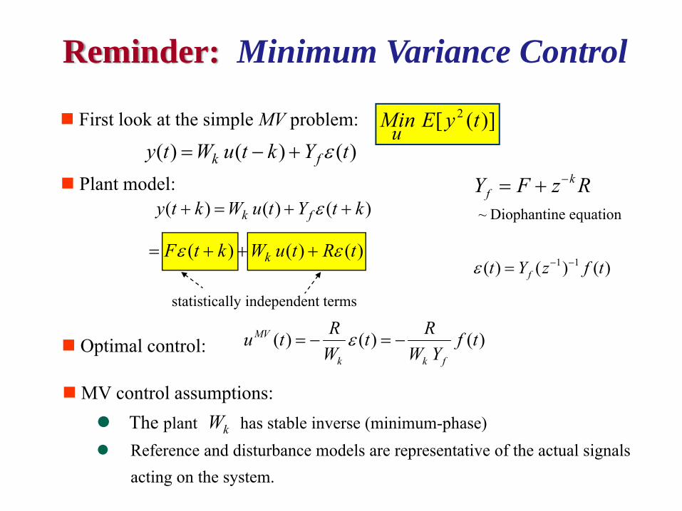
Reminder: Minimum Variance Control

First look at the simple MV problem: 2[ ( )]uMin E y t

( ) ( ) ( )k fy t k W u t Y t kε+ = + +

Optimal control: ( ) ( ) ( )MV

k k f

R Ru t t f tW W Y

ε= − = −

kfY F z R−= +

statistically independent terms

~ Diophantine equation

MV control assumptions:The plant has stable inverse (minimum-phase)Reference and disturbance models are representative of the actual signals acting on the system.

Plant model:

( ) ( ) ( )k fy t W u t k Y tε= − +

( ) ( ) ( )kF t k W u t R tε ε= + + +1 1( ) ( ) ( )ft Y z f tε − −=

kW

Nonlinear Generalised Minimum Variance Control

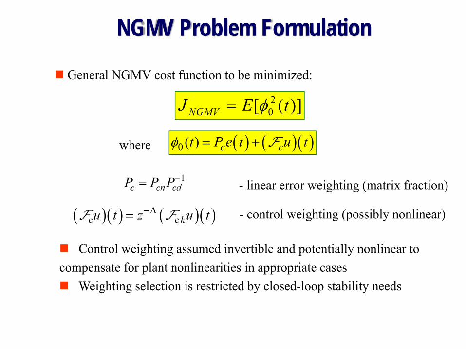
NGMV Problem Formulation

Control weighting assumed invertible and potentially nonlinear to compensate for plant nonlinearities in appropriate cases

Weighting selection is restricted by closed-loop stability needs

20[ ( )]NGMVJ E tφ=

( )( ) ( )( )c c ku t z u t−Λ=F F

1c cn cdP P P−= - linear error weighting (matrix fraction)

General NGMV cost function to be minimized:

where

- control weighting (possibly nonlinear)

( ) ( )( )0 ( ) c ct P e t u tφ = + F

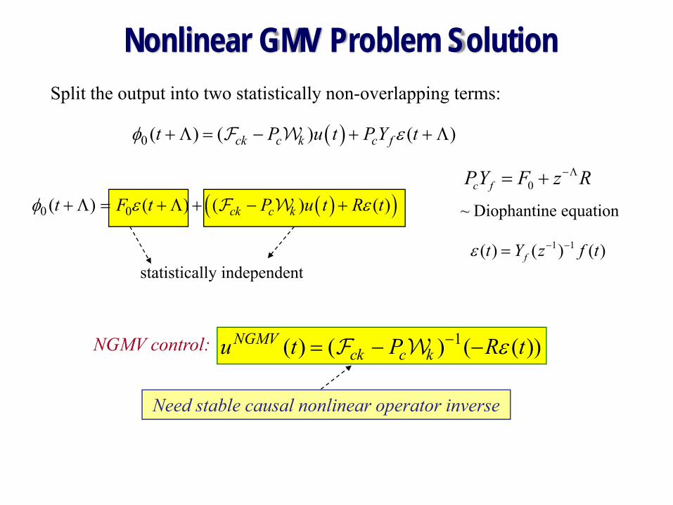
Nonlinear GMV Problem Solution

0c fPY F z R−Λ= +( )( )0 0( ) ( ) ( ) ( )ck c kt F t P u t R tφ ε ε+ Λ = + Λ + − +F W

statistically independent

1( ) ( ) ( ( ))NGMVck c ku t P R tε−= − −F W

Need stable causal nonlinear operator inverse

~ Diophantine equation

Split the output into two statistically non-overlapping terms:

NGMV control:

( )0 ( ) ( ) ( )ck c k c ft P u t P Y tφ ε+ Λ = − + + ΛF W

1 1( ) ( ) ( )ft Y z f tε − −=

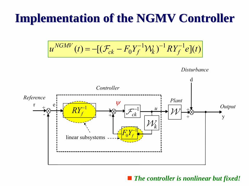
Implementation of the NGMV Controller

1 1 10( ) [( ) ]( )NGMV

ck f k fu t F Y RY e t− − −= − −F W

d

++u-

+

Controller

Disturbance

eReference

OutputPlant

y+-

r 1fRY− 1

ck−F

kWW

10 fFY−

linear subsystems

ψ

The controller is nonlinear but fixed!

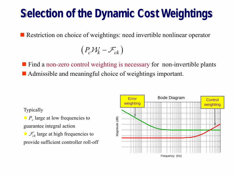
Selection of the Dynamic Cost WeightingsRestriction on choice of weightings: need invertible nonlinear operator

( )c k ckP −W F

Find a non-zero control weighting is necessary for non-invertible plantsAdmissible and meaningful choice of weightings important.

TypicallyPc large at low frequencies to

guarantee integral action Fck large at high frequencies to

provide sufficient controller roll-off

Mag

nitu

de (d

B)

Bode Diagram

Frequency (Hz)

Errorweighting

Controlweighting

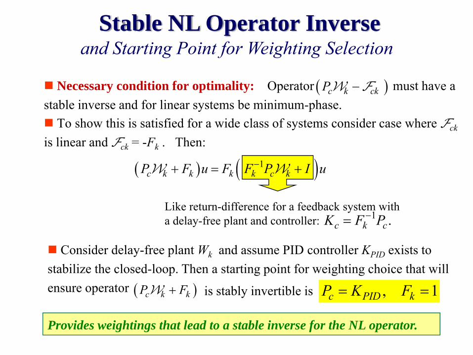
Necessary condition for optimality: Operator must have a stable inverse and for linear systems be minimum-phase.

To show this is satisfied for a wide class of systems consider case where Fck

is linear and Fck = -Fk . Then:

( )c k ckP −W F

( ) ( )1c k k k k c kP F u F F P I u−+ = +W W

1 .c k cK F P−=

Stable NL Operator Inverse and Starting Point for Weighting Selection

Like return-difference for a feedback system witha delay-free plant and controller:

Consider delay-free plant Wk and assume PID controller KPID exists to stabilize the closed-loop. Then a starting point for weighting choice that will ensure operator ( )c k kP F+W is stably invertible is , 1c PID kP K F= =

Provides weightings that lead to a stable inverse for the NL operator.

Predictive Controller For Nonlinear Processes:

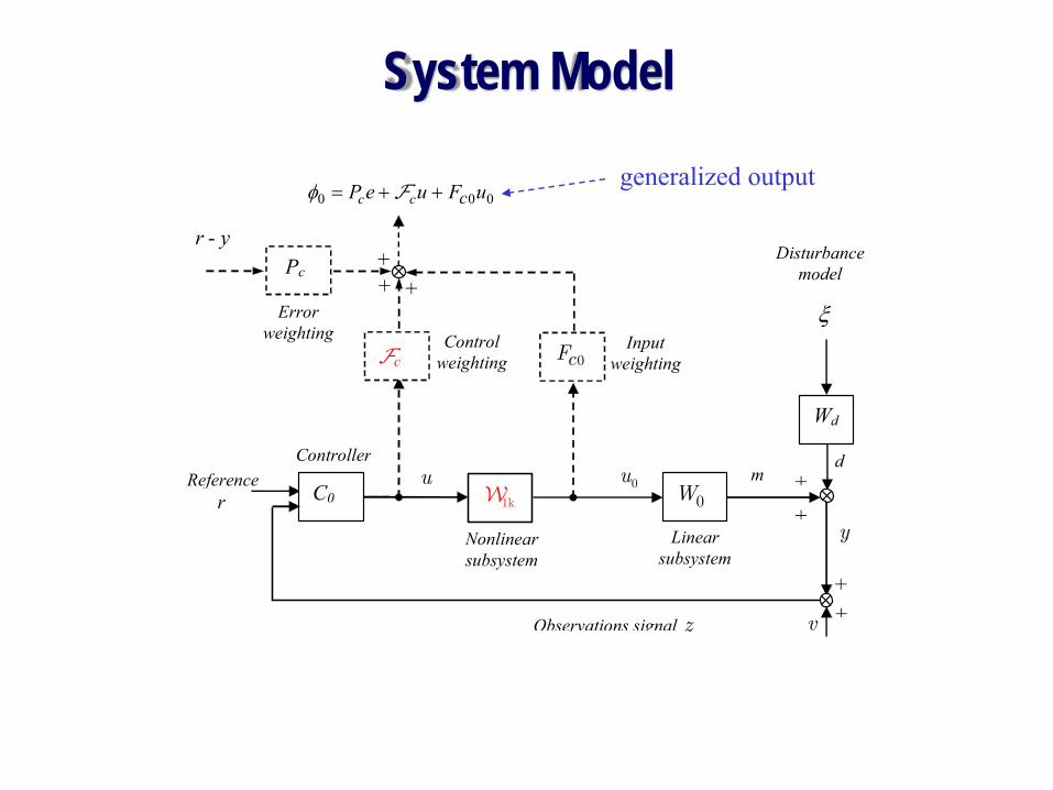
System Model

Disturbancemodel

0 0 0c c cP e u F uφ = + +F

v

Pc

Wd

r u

y

d

1kW

+

+m

Fc Control

weighting

Reference

Error weighting

+ξ

C0

Nonlinearsubsystem

Controller

0W0u

0cF

+

Input weighting

Linear subsystem

+

+

Observations signal z

+

-r y

generalized output

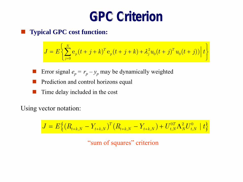
GPC Criterion

λ=

⎧ ⎫= + + + + + + +⎨ ⎬

⎩ ⎭∑ 2

0 00

e ( ) e ( ) ( ) ( ))N

T Tp p j

j

J E t j k t j k u t j u t j t

Typical GPC cost function:

Error signal ep = rp – yp may be dynamically weighted

Prediction and control horizons equal

Time delay included in the cost

{ }+ + + += − − + Λ0 2 0, , , , , ,( ) ( ) |T T

t k N t k N t k N t k N t N N t NJ E R Y R Y U U t

Using vector notation:

“sum of squares” criterion

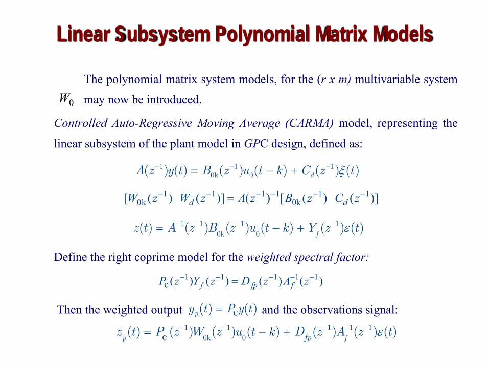
Linear Subsystem Polynomial Matrix Models

The polynomial matrix system models, for the (r x m) multivariable system

may now be introduced.

Controlled Auto-Regressive Moving Average (CARMA) model, representing the

linear subsystem of the plant model in GPC design, defined as:

Define the right coprime model for the weighted spectral factor:

Then the weighted output and the observations signal:

0W

ξ− − −= − +1 1 10k 0( ) ( ) ( ) ( ) ( ) ( )dA z y t B z u t k C z t

1 1 1 1 1 10k 0k[ ( ) ( )] ( ) [ ( ) ( )]d dW z W z A z B z C z− − − − − −=

ε− − − −= − +1 1 1 10k 0

( ) ( ) ( ) ( ) ( ) ( )f

z t A z B z u t k Y z t

1 1 1 1 1c( ) ( ) ( ) ( )f fp fP z Y z D z A z− − − − −=

ε− − − − −= − +1 1 1 1 10k 0c( ) ( ) ( ) ( ) ( ) ( ) ( )

p ffpz t P z W z u t k D z A z t

c( ) ( )py t P y t=

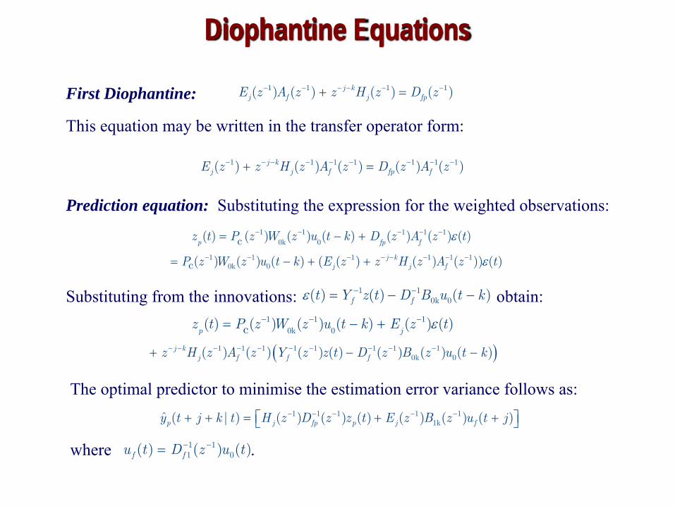
Diophantine Equations

First Diophantine:

This equation may be written in the transfer operator form:

Prediction equation: Substituting the expression for the weighted observations:

Substituting from the innovations: obtain:

1 1 1 1( ) ( ) ( ) ( )j kj f j fpE z A z z H z D z− − − − − −+ =

1 1 1 1 1 1 1( ) ( ) ( ) ( ) ( )j kj j f fp fE z z H z A z D z A z− − − − − − − − −+ =

ε− − − − −= − +1 1 1 1 10k 0c( ) ( ) ( ) ( ) ( ) ( ) ( )

p fp fz t P z W z u t k D z A z t

1 1 1 1 1 10k 0c( ) ( ) ( ) ( ( ) ( ) ( )) ( )j k

j j fP z W z u t k E z z H z A z tε− − − − − − − −= − + +

1 10k 0( ) ( ) ( )f ft Y z t D B u t kε − −= − −

ε− − −= − +1 1 10k 0c( ) ( ) ( ) ( ) ( ) ( )

p jz t P z W z u t k E z t

( )1 1 1 1 1 1 1 10k 0( ) ( ) ( ) ( ) ( ) ( ) ( )j k

j f f fz H z A z Y z z t D z B z u t k− − − − − − − − − −+ − −

The optimal predictor to minimise the estimation error variance follows as:

where .

1 1 1 1 11kˆ ( | ) ( ) ( ) ( ) ( ) ( ) ( )p j fp p j fy t j k t H z D z z t E z B z u t j− − − − −⎡ ⎤+ + = + +⎣ ⎦

1 11 0( ) ( ) ( )f fu t D z u t− −=

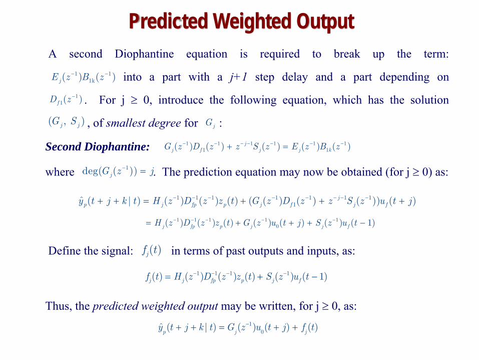
Predicted Weighted OutputA second Diophantine equation is required to break up the term:

into a part with a j+1 step delay and a part depending on

. For j ≥ 0, introduce the following equation, which has the solution

, of smallest degree for :

Second Diophantine:

where . The prediction equation may now be obtained (for j ≥ 0) as:

Define the signal: in terms of past outputs and inputs, as:

Thus, the predicted weighted output may be written, for j ≥ 0, as:

1 11k( ) ( )jE z B z− −

( , )j jG SjG

1 1 1 1 1 11 1( ) ( ) ( ) ( ) ( )j

j f j j kG z D z z S z E z B z− − − − − − −+ =

1deg( ( ))jG z j− =

1 1 1 1 1 1 11ˆ ( | ) ( ) ( ) ( ) ( ( ) ( ) ( )) ( )j

p j fp p j f j fy t j k t H z D z z t G z D z z S z u t j− − − − − − − −+ + = + + +

1 1 1 1 10( ) ( ) ( ) ( ) ( ) ( ) ( 1)j fp p j j fH z D z z t G z u t j S z u t− − − − −= + + + −

11( )fD z −

( )jf t

1 1 1 1( ) ( ) ( ) ( ) ( ) ( 1)j j fp p j ff t H z D z z t S z u t− − − −= + −

−+ + = + +10

ˆ ( | ) ( ) ( ) ( )p j jy t j k t G z u t j f t

Matrix Representation of the Prediction Equations

The future weighted outputs are to be predicted in the following section for

inputs computed in the interval: . The equation may therefore be

used to obtain the following vector equation for the weighted output at future times:

[ , ]t t Nτ ε +

0 0 0

1 0 0 1

1 0

1 0 0

ˆ 0 0 0( | ) ( ) ( )

0 0ˆ ( 1 | ) ( 1) ( )

ˆ ( | ) ( ) ( )

p

p

N Np N

gy t k t u t f t

g gy t k t u t f t

g g

g g gy t N k t u t N f t−

+⎡ ⎤ ⎡ ⎤ ⎡ ⎤⎡ ⎤⎢ ⎥ ⎢ ⎥ ⎢ ⎥⎢ ⎥+ + +⎢ ⎥ ⎢ ⎥ ⎢ ⎥⎢ ⎥⎢ ⎥ ⎢ ⎥ ⎢ ⎥⎢ ⎥= +⎢ ⎥ ⎢ ⎥ ⎢ ⎥⎢ ⎥⎢ ⎥ ⎢ ⎥ ⎢ ⎥⎢ ⎥⎢ ⎥ ⎢ ⎥ ⎢ ⎥⎢ ⎥

+ + +⎢ ⎥ ⎢ ⎥ ⎢ ⎥⎢ ⎥⎣ ⎦⎣ ⎦ ⎣ ⎦ ⎣ ⎦…

Vector Form of Prediction Equations

Introducing an obvious definition of terms for the matrices in the above

equation the vector form of the predicted weighted outputs may be written as:

The vector of free response predictions may also be written as:

0, , ,t̂ k N N t N t NY G U F+ = +

,t NF

1 10 00

1 11 1 11 1

1 1

( ) ( )( )

( ) ( ) ( )( ) ( ) ( 1)

( ) ( ) ( )

fp p f

N N N

H z S zf t

f t H z S zD z z t u t

f t H z S z

− −

− −

− −

− −

⎡ ⎤ ⎡ ⎤⎡ ⎤⎢ ⎥ ⎢ ⎥⎢ ⎥⎢ ⎥ ⎢ ⎥⎢ ⎥

= = + −⎢ ⎥ ⎢ ⎥⎢ ⎥⎢ ⎥ ⎢ ⎥⎢ ⎥⎢ ⎥ ⎢ ⎥⎢ ⎥⎢ ⎥ ⎢ ⎥⎣ ⎦ ⎣ ⎦ ⎣ ⎦

1 1( ) ( ) ( ) ( 1)NZ p NZ fH z z t S z u t− −= + −

,t NF

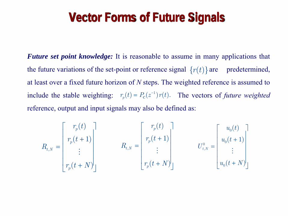
Vector Forms of Future Signals

Future set point knowledge: It is reasonable to assume in many applications that

the future variations of the set-point or reference signal are predetermined,

at least over a fixed future horizon of N steps. The weighted reference is assumed to

include the stable weighting: The vectors of future weighted

reference, output and input signals may also be defined as:

{ ( )}r t

1c( ) ( ) ( ).pr t P z r t−=

,

( )

( 1)

( )

p

p

t N

p

r t

r tR

r t N

⎡ ⎤⎢ ⎥

+⎢ ⎥= ⎢ ⎥⎢ ⎥⎢ ⎥+⎣ ⎦

,

( )

( 1)

( )

p

p

t N

p

r t

r tR

r t N

⎡ ⎤⎢ ⎥

+⎢ ⎥= ⎢ ⎥⎢ ⎥⎢ ⎥+⎣ ⎦

0

00,

0

( )

( 1)

( )

t N

u t

u tU

u t N

⎡ ⎤⎢ ⎥

+⎢ ⎥= ⎢ ⎥⎢ ⎥⎢ ⎥+⎣ ⎦

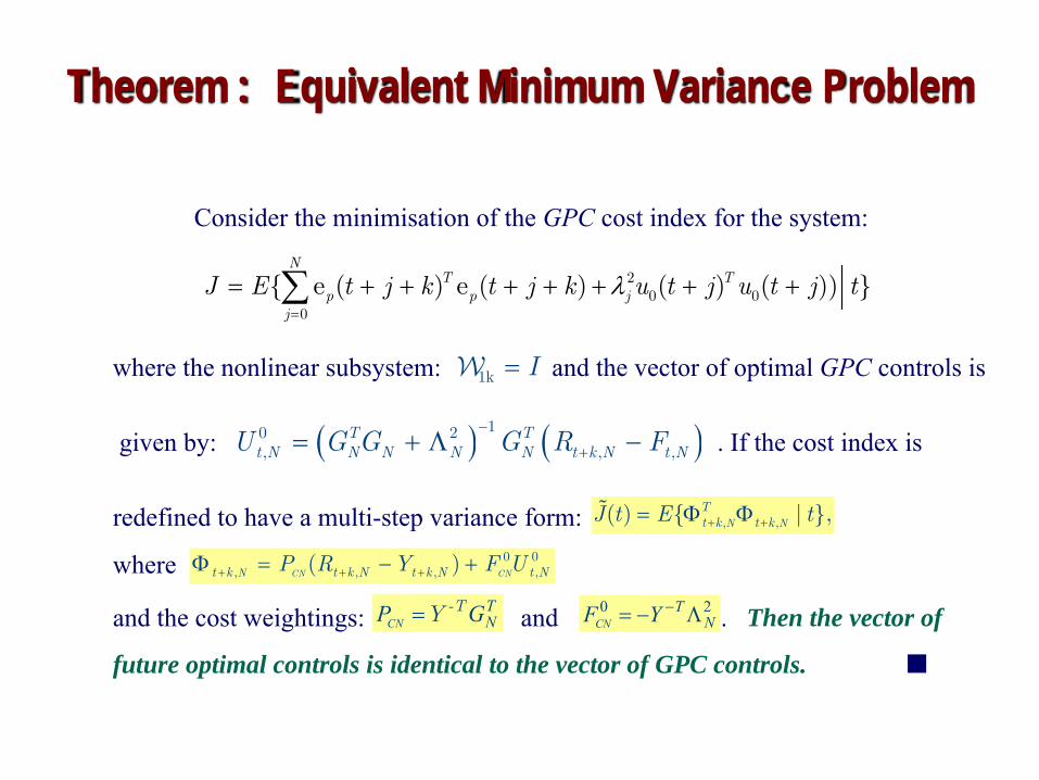
Theorem : Equivalent Minimum Variance Problem

Consider the minimisation of the GPC cost index for the system:

where the nonlinear subsystem: and the vector of optimal GPC controls is

given by: . If the cost index is

redefined to have a multi-step variance form:

where

and the cost weightings: and . Then the vector of

future optimal controls is identical to the vector of GPC controls. ■

, ,( ) { | },N NTt k t kJ t E t+ += Φ Φ

0 0, , , ,( )

CN CNNt k t k N t k N t NP R Y F U+ + +Φ = − +

0 2−= − ΛCNT

NF Y-TY=CNTNP G

1k I=W

λ=

= + + + + + + +∑ 20 0

0

{ e ( ) e ( ) ( ) ( )) }N

T Tp p j

j

J E t j k t j k u t j u t j t

( ) ( )10 2, , ,

T Tt N N N N N t k N t NU G G G R F

−

+= + Λ −

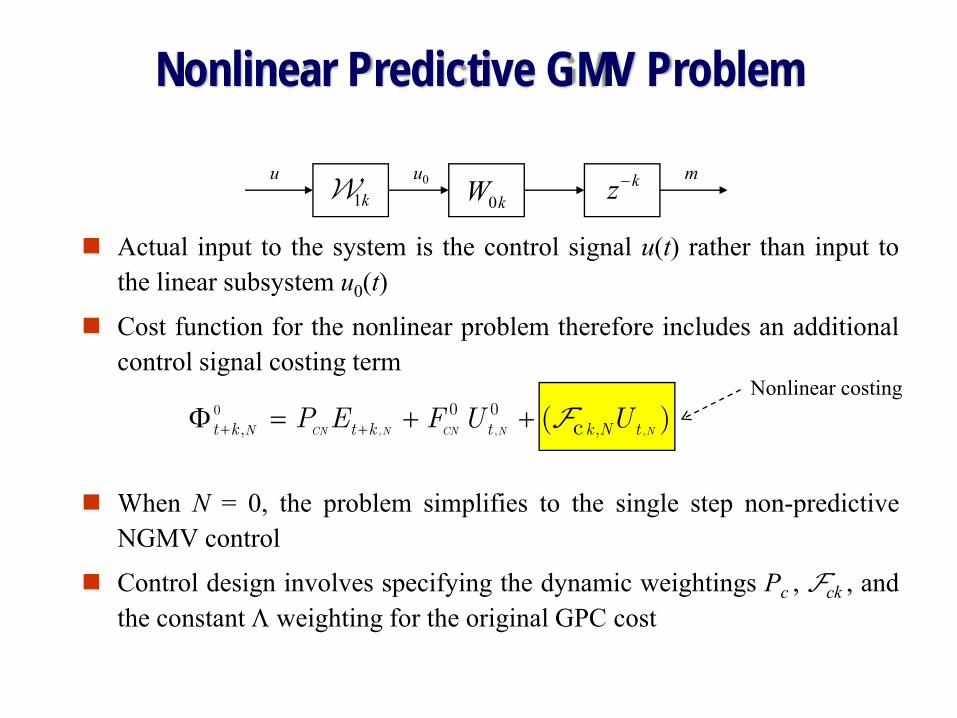
Nonlinear Predictive GMV Problem

Actual input to the system is the control signal u(t) rather than input tothe linear subsystem u0(t)

Cost function for the nonlinear problem therefore includes an additionalcontrol signal costing term

Nonlinear costing

+ +Φ = + +, , ,

0 0 0, ,c( )

CN N CN N NNt k t k t k N tP E F U UF

1kW 0kW kz−u0u m

When N = 0, the problem simplifies to the single step non-predictiveNGMV control

Control design involves specifying the dynamic weightings Pc , Fck , andthe constant Λ weighting for the original GPC cost

Let error weighting and the input weightings be specified and

assume the control signal weighting: where is full rank

and invertible. The multi-step cost-function:

The signal includes the vector of future error, input and control signal costing

terms: where the effective weightings :

, and may be a diagonal control weighting.

Define the constant matrix factor Y to satisfy then using the

receding horizon philosophy the control law:

or equivalently:

where the signals: and

ckF0 0, ,{ | }N N

Tp t k t kJ E t+ += Φ Φ

0{ ,..., }Nλ λ

( )( ) ( )( )c c= −ku t u t kF F

1( )cP z−

0,Nt k+Φ

, , ,

0 0 0, ,c( )

CN N CN N NNt k t k t k N tP E F U U+ +Φ = + + F

-TY=CNTNP G 0 2−= − ΛCN

TNF Y ,ck NF

= + Λ2TN

TN NY G GY

−+= − − −

,

1, 1k,N , ,c( ) ( )

N CNt k N t k N t NU Y P R FF W

( )+= − − −, ,

-1, , , 1k,Nc ( )

N CN Nt k N t k N t N tU P R F Y UF W

− −= + −t N NZ NZ fF H z z t S z u t1 1, ( ) ( ) ( ) ( 1)

− −= 1 11 0( ) ( ) ( ).f fu t D z u t

Theorem: NL Predictive GMV Control

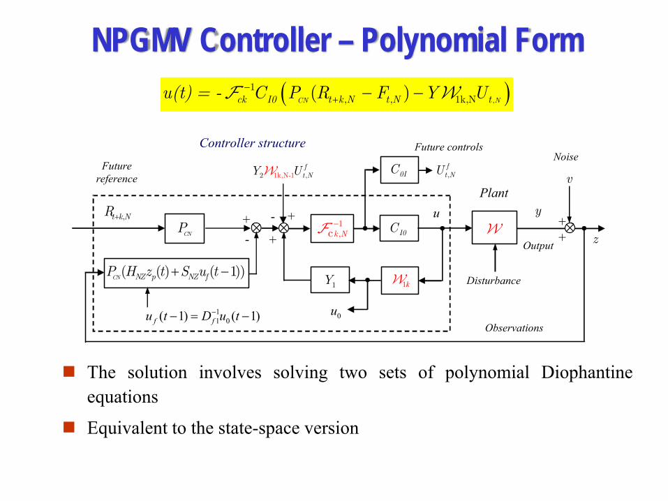
NPGMV Controller – Polynomial Form

Future

reference

+ ,t k NR

Future controls

Observations

u-

Controller structure

Disturbance

Plant

W + z

I0C−1,ck NF

0IC ,ft NU

1kW 1Y

CNP

( ( ) ( 1))CN NZ p NZ fP H z t S u t+ −

+- +

+

v

Noise

y

0u 11 0( 1) ( 1)−− = −f fu t D u t

Output

W1k,N-2 ,1ft NY U

+

( ),

1, , 1k,N( )

CN Nck I0 t k N t N tu(t) = - C P R F Y U−+ − −F W

The solution involves solving two sets of polynomial Diophantineequations

Equivalent to the state-space version

Robotics Application of Nonlinear Predictive Control

m1, I1

q1

q2

τ1

τ2

l1

lc1

lce

δe

me, Ie

Robotics Application Two-link robotic manipulator

After "Applied Nonlinear Control" by Slotine and Li, 1991.

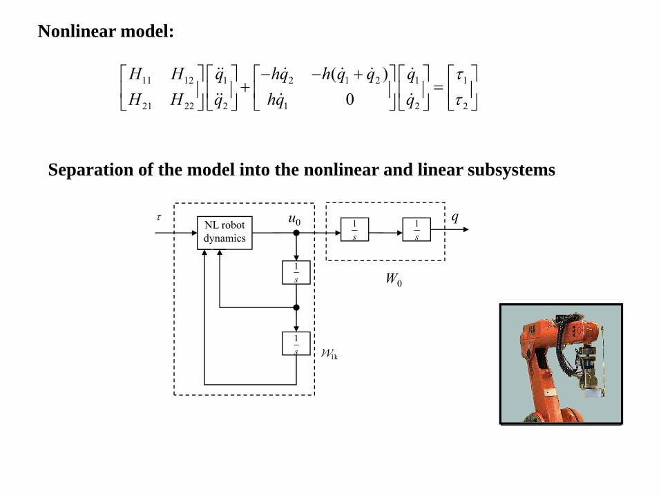
11 12 1 2 1 2 1 1

21 22 2 1 2 2

( )0

H H q hq h q q qH H q hq q

ττ

− − +⎡ ⎤ ⎡ ⎤ ⎡ ⎤ ⎡ ⎤ ⎡ ⎤+ =⎢ ⎥ ⎢ ⎥ ⎢ ⎥ ⎢ ⎥ ⎢ ⎥

⎣ ⎦ ⎣ ⎦ ⎣ ⎦ ⎣ ⎦ ⎣ ⎦

Nonlinear model:

NL robotdynamics

qu0

W0

τ

W1k

1s

1s

1s

1s

Separation of the model into the nonlinear and linear subsystems

NPGMV controller structure for robot control

Position Control of the Two-link manipulator. NPGMV control with N = 0, 1, 3, 5 and Feedback linearization

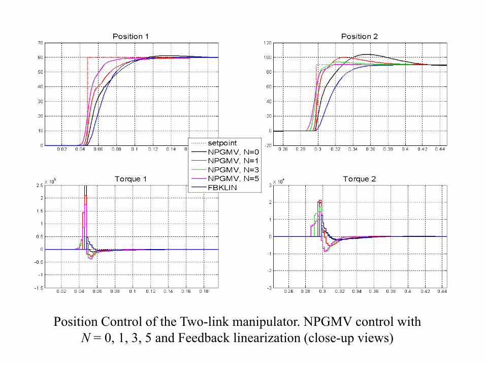
Position Control of the Two-link manipulator. NPGMV control with N = 0, 1, 3, 5 and Feedback linearization (close-up views)

Marine Systems Roll Stabilization Example

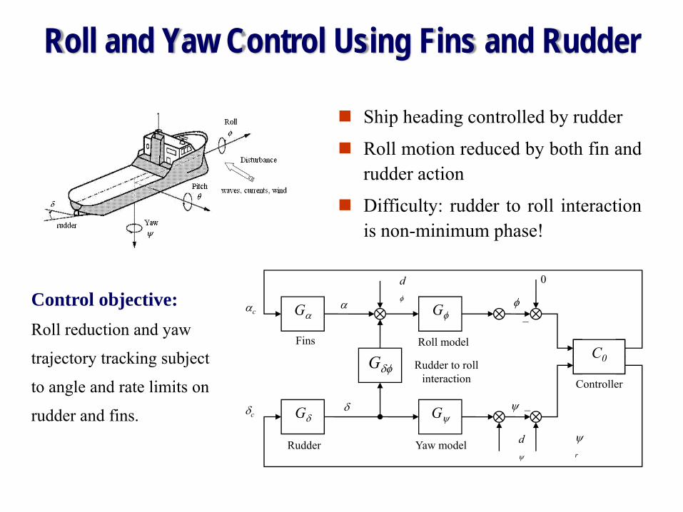
Roll and Yaw Control Using Fins and Rudder

Gφ

Gψ

Gδφ

Gδ

Gα

C0

φ

ψ

ψr

δδc

ααc

0

−

−

dφ

dψ

Fins

Rudder

Roll model

Yaw model

Rudder to roll interaction Controller

Ship heading controlled by rudder

Roll motion reduced by both fin andrudder action

Difficulty: rudder to roll interactionis non-minimum phase!

Control objective:Roll reduction and yaw

trajectory tracking subject

to angle and rate limits on

rudder and fins.

Ship Roll Stabilisation Problem

10-1

100

-10

-8

-6

-4

-2

0

2

4M

agni

tude

(dB)

Frequency (rad/sec)

~20 dB

< 5 dB(1) Achieve good roll stabilization(2) Do not hit rudder constraints(3) Keep the vessel on course

Compensate roll motion in a well-defined frequency band (0.3-1.2 rad/sec)

LF rejection may cause rudder angle saturation

HF rejection may cause rudder slew rate saturation

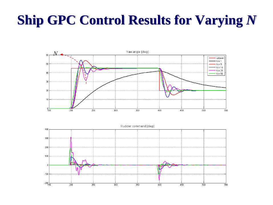
Ship GPC Control Results for Varying N

N

Example: GPC and NPGMV Results

Open Loop

GPC

NPGMV

Concluding Remarks

A practical NL controller must be simple but we need some mathematical basis to understand behavior. NGMV is a candidate and the patriarch for a family of more complicated and specialist solutions.The ability to handle black box models is important industrially.Nonlinear predictive is a model based fixed controller without uncertainty of linearization around a trajectory - so interesting.Extendable further to hybrid and/or complex systems.LabVIEW toolbox including new tools next !Dual Estimation problems equally interesting.

Nonlinear Book

Dr Pawel MajeckiIndustrial Control CentreUniversity of StrathclydeDepartment of Electronic and Electrical EngineeringGraham Hills Building50 George StreetGlasgow G1 1QE, UKE-mail: p.majecki@eee.strath.ac.ukTelephone No: +44 (0)141 552 4400 Extensions: 2378Direct Line No: +44 (0)141 548 2378Facsimile No: +44 (0)141 548 4203http://www.icc.strath.ac.uk

For new book on nonlinear control, to be published next year: M. J. Grimble and P. Majecki, Nonlinear Industrial Control,

Springer, Heidelberg, Germany 2009