Simple Identification and Specification of Cointegrated

VARMA Models ∗

Christian Kascha† Carsten Trenkler‡

University of Zurich University of Mannheim

January 22, 2014

Abstract

We bring together some recent advances in the literature on vector autoregressivemoving-average models creating a simple specification and estimation strategy for thecointegrated case. We show that in this case with fixed initial values there exists a so-called final moving-average representation. We proof that the specification strategy isconsistent. The performance of the proposed method is investigated via a Monte Carlostudy and a forecasting exercise for US interest rates. We find that our method performswell relative to alternative approaches for cointegrated series and methods which do notallow for moving-average terms.

JEL classification: C32, C53, E43, E47Keywords: Cointegration, VARMA Models, Forecasting

1 Introduction

In this paper, we propose a relatively simple specification and estimation strategy for thecointegrated vector autoregressive moving-average (VARMA) model using the estimatorsgiven in Yap and Reinsel (1995), Poskitt and Lutkepohl (1995), and Poskitt (2003) and theidentified forms proposed by Dufour and Pelletier (2011). We investigate the performanceof the proposed methods via a Monte Carlo study and a forecasting exercise for US interestrates and find promising results.

The motivation for looking at this particular model class stems from the well-known the-oretical advantages of VARMA models over pure vector-autoregressive (VAR) processes; seee.g. Lutkepohl (2005). In contrast to VAR models, the class of VARMA models is closedunder linear transformations. For example, a subset of variables generated by a VAR process

∗We thank two anonymous referees, the co-editor, Francesco Ravazzolo, Kyusang Yu, Michael Vogt and sem-inars participants at the Tinbergen Institute Amsterdam, Universities of Aarhus, Bonn, Konstanz, Mannheim,and Zurich as well as session participants at the ISF 2011, Prague, at the ESEM 2011, Oslo, and at the NewDevelopments in Time Series Econometrics conference, Florence, for very helpful comments.†University of Zurich, Chair for Statistics and Empirical Economic Research, Zurichbergstrasse 14, 8032

Zurich, Switzerland; christian.kascha@econ.uzh.ch‡Address of corresponding author: University of Mannheim, Department of Economics, Chair of Empir-

ical Economics, L7, 3-5, 68131 Mannheim, Germany; Phone: +49-621-181-1845; Fax: +49-621-181-1931;trenkler@uni-mannheim.de

1

is typically generated by a VARMA, not by a VAR process (Lutkepohl, 1984a,b). It is wellknown that linearized dynamic stochastic general equilibrium (DSGE) models imply that thevariables of interest are generated by a finite-order VARMA process. Fernandez-Villaverde,Rubio-Ramırez, Sargent and Watson (2007) show formally how DSGE models and VARMAprocesses are linked. Cooley and Dwyer (1998) claim that modeling macroeconomic timeseries systematically as pure VARs is not justified by the underlying economic theory. Acomparison of structural identification methods using VAR, VARMA and state space repre-sentations is provided by Kascha and Mertens (2009).

Existing specification and estimation procedures for cointegrated VARMA models con-sider sets of parameter restrictions, such as the so-called echelon form or the scalar-componentrepresentation, which make sure that the remaining free parameters are identified with re-spect to the likelihood function. However, while both identified forms can yield represen-tations which are relatively parsimonious, they are often overly complex. Approaches forcointegrated VARMA models that use the (reverse) echelon form can be found in Yap andReinsel (1995); Lutkepohl and Claessen (1997); Poskitt (2003, 2006) and also Poskitt (2009).The scalar-component representation was originally proposed by Tiao and Tsay (1989) andembedded in a complete estimation procedure by Athanasopoulos and Vahid (2008).

Instead, we extend the final moving-average (FMA) representation of Dufour and Pel-letier (2011) to the cointegrated case with fixed initial values. The FMA representation onlyimposes restrictions on the MA part of the model and, therefore, has a simpler structurethan the echelon form. Furthermore, we propose to specify the model using Dufour andPelletier’s (2011) order selection criterion applied to the model estimated in levels. We proofa.s. consistency of the estimated orders in this case.

In addition, we compared the proposed approach to the existing approaches via MonteCarlo simulations and via a forecasting exercise. In particular, we apply the methods tothe problem of predicting U.S.treasury bill and bond interest rates with different maturitiestaking cointegration as given. We find rather promising results relative to a variety of differ-ent models including a multivariate random walk, the standard vector error correction model(VECM) and approaches based on the echelon form. An investigation of the relative forecast-ing performances over time shows that our cointegrated VARMA model delivers consistentlygood forecasts apart from a period stretching from the mid-nineties to 2000.

The rest of the paper is organized as follows. Section 2 discusses our proposals for theidentification, specification and estimation of cointegrated VARMA models. In Section 3we present the results on a Monte Carlo study that investigates how one should implementthe proposed procedures and how these compare to alternative methods. Section 4 containsthe forecasting study and Section 5 concludes. All programs and data can be found on thehomepages of the authors.

2 Cointegrated VARMA models

2.1 Model Framework

The data generating process is formulated here. The assumptions we impose allow us touse the results of Yap and Reinsel (1995), Poskitt and Lutkepohl (1995), Poskitt (2003) andDufour and Pelletier (2011) in order to construct a reasonably easy and fast strategy for thespecification and estimation of cointegrated VARMA models. The considered model for a

2

time series of dimension K, yt = (yt,1, . . . , yt,K)′, is

A0yt =

p∑j=1

Ajyt−j +

q∑j=0

Mjut−j for t = 1, . . . , T, (1)

where Aj , j = 1, . . . , p, and Mj , j = 1, . . . , q are K × K parameter matrices with Ap 6= 0and Mq 6= 0 and m := max{p, q}. The initial values y1−m, . . . , y0 are assumed to be fixedconstants.

Let us also define the matrix polynomials A(z) := A0 − A1z − A2z2 − . . . − Apzp and

M(z) := M0 + M1z + . . . + Mqzq, z ∈ C, with A0 and M0 being invertible, and a pair

of these by [A(z),M(z)]. Using the notation from Poskitt (2006) with minor modifica-tions, we define deg[A(z), M(z)] as the maximum row degree max1≤k≤K degk[A(z), M(z)],where degk[A(z), M(z)] denotes the polynomial degree of the kth row of [A(z), M(z)].Then we can define a class of processes by its associated set {[AM ]}m := {[A(z), M(z)] :deg[A(z), M(z)] = m}.

Regarding the error terms we make the following assumption which is equivalent to As-sumption A.2 in Poskitt (2003).

Assumption 2.1 The error term vectors ut = (u′t,1, u′t,2, . . . , u

′t,K), t = 1−m, . . . , 0, 1, . . . , T ,

form an independent, identically distributed zero mean white noise sequence with positive defi-nite variance-covariance matrix Σu. Furthermore, the moment condition E

(||ut||δ1

)<∞ for

some δ1 > 2, where || · || denotes the Euclidean norm, and growth rate ||ut|| = O((log t)1−δ2)

)almost surely (a.s.) for some 0 < δ2 < 1 also hold.

We make the following two assumptions regarding the polynomials A(z) and M(z):

Assumption 2.2 |M(z)| 6= 0 for |z| ≤ 1, z ∈ C, where | · | refers to the determinant.

Assumption 2.3 The components in yt are at most integrated of order one such that ∆yt =yt − yt−1 is asymptotically stationary. Moreover, |A(z)| = ast(z)(1− z)s for 0 < s ≤ K andast(z) 6= 0 for |z| ≤ 1, z ∈ C. The number r = K − s is called the cointegrating rank of theseries yt.

Hence, the moving-average polynomial is assumed to be invertible. Moreover, it followsfrom Assumption 2.3 that we can decompose Π :=

∑pj=1Aj − A0 as Π = αβ′, where α and

β are (K × r) matrices with full column rank r. Thus, one can write

A0∆yt = αβ′yt−1 +

p−1∑j=1

Γj∆yt−j +

q∑j=0

Mjut−j (2)

with Γj = −(Aj+1 + · · ·+Ap), t = 1, . . . , T .We have not considered a constant term in the specification in (1), mainly for nota-

tional convenience. The used estimation methods remain valid provided the constant canbe absorbed in the cointegrating relation, i.e. if a constant term in (1) can be expressed asµ0 = −αρ, where ρ is of dimension r × 1, such that a linear trend in the variables is ruledout; see Poskitt (2003, Section 2, p. 507) and Yap and Reinsel (1995, Section 6). We followthe approach of Poskitt (2003) and Yap and Reinsel (1995) to accommodate such a constantterm by mean-adjusting the data prior to estimation and specification. Hence, we actually

3

apply the methods to yt − T−1∑T

s=1 ys in the VARMA case. However, the notation in thefollowing will not distinguish between raw and adjusted data. The explicit inclusion of aconstant term into the estimation procedure is discussed in Lutkepohl and Claessen (1997).

2.2 Identification

It is well known, that one has to impose certain restrictions on the parameter matrices inorder to achieve uniqueness. That is, given a series (yt)

Tt=1−m, there is generally more than

one pair of finite polynomials [A(z), M(z)] such that (1) is satisfied. Therefore, one has torestrict the set of considered pairs [A(z), M(z)] to a subset such that every process satisfying(1) is represented by exactly one pair in this subset.

Poskitt (2003) proposes a complete modeling strategy using the echelon form which isbased on so-called Kronecker indices. Here, we use the much simpler final moving-average(FMA) representation proposed by Dufour and Pelletier (2011) in the context of stationaryVARMA models. This representation imposes restrictions on the moving-average polynomialonly. More precisely, we consider only polynomials [A(z), M(z)], such that

M(z) = m(z)IK , m(z) = 1 +m1z + . . .+mqzq. (3)

is true and choose among these the pair with the smallest possible orders p, q.1 As alreadynoted by Dufour and Pelletier (2011), this identification strategy is valid despite A(z) havingroots on the unit circle. What is left, is only to show the existence and uniqueness of theFMA form in the non-stationary context with fixed initial values. Analogous to the resultsin Poskitt (2006), we can show that in this particular case the resulting pair of polynomialsdoes not have to be left-coprime anymore. We assume

Assumption 2.4 The K-dimensional series (yt)Tt=1−m admits a VARMA representation as

in (1) with A0 = M0, [A(z), M(z)] ∈ {[AM ]}m and fixed initial values y1−m, . . . , y0.

The identification of the parameters of the FMA form follows from the observation thatany process that satisfies (1) can always be written as

yt =t+m−1∑s=1

Πsyt−s + ut + nt, t = 1−m, . . . , T, (4)

where it holds, by construction of the sequences (Πi)T+m−1i=0 and (nt)

Tt=1−m, that

0 =m∑j=0

MjΠi−j , i > m (5)

0 =

m∑j=0

Mjnt−j , t ≥ 1. (6)

1 Dufour and Pelletier (2011) also propose another representation that restricts attention to pairs withdiagonal moving-average polynomials such as M(z) = diag(m1(z), m2(z), . . . , mK(z)) where mk(z) = 1 +mk,1z + . . .mk,qkz

qk k = 1, . . . , K are scalar polynomials. This form delivered results similar to the ones forthe FMA form and will therefore not be discussed in the paper.

4

On the other hand, given a process satisfying (4) and existence of matricesM0, M1, . . . , Mm

such that conditions (5) and (6) are true, the process has a VARMA representation as above.These statements are made precise in the following theorem which is just a restatement ofthe corresponding theorem in Poskitt (2006).

Theorem 2.1 The process (yt)Tt=1−m admits a VARMA representation as in (1) with A0 =

M0, A0 invertible, [A(z), M(z)] ∈ {[A M ]}m and initial conditions y0, . . . , y1−m if and onlyif (yt)

Tt=1−m admits an autoregressive representation

yt =

t+m−1∑s=1

Πsyt−s + ut + nt, t = 1−m, . . . , T,

and there exist matrices M0,M1, . . . ,Mm which satisfy conditions (5) and (6) and M0 isinvertible.

Now, one assigns to the autoregressive representation a unique VARMA representation.Because of the properties of the adjoint, Mad(z)M(z) = |M(z)|, equations (5) and (6) imply

0 =

q∑j=0

mjΠi−j , i > q (7)

0 =

q∑j=0

mjnt−j , t ≥ q −m+ 1. (8)

Here, |M(z)| =: m(z) = m0 + m1z + . . . + mqzq is a scalar polynomial and q = m ·K is its

maximal order.Because of Theorem 2.1, one can therefore define a pair in final moving-average form as in

(3), [A(z), m(z)IK ], provided that T ≥ q −m+ 1 and that the first coefficient is normalizedto one. This representation, however, is not the only representation of this form. To achieveuniqueness, we select the representation of the form [A(z), m(z)IK ] with the lowest possibledegree of the scalar polynomial m(z) such that the first coefficient is normalized to one and(7) and (8) are satisfied.

Theorem 2.2 Assume that the process (yt)Tt=1−m satisfies Assumption 2.2 and 2.4. Then,

for T ≥ q−m+ 1, it is always possible to select an observationally equivalent, representationin terms of a pair [A0(z), m0(z)IK ] with A0 = IK and minimal orders p0 and q0 commencingfrom some t0 ≥ 1−m.

In contrast to the discussion in Dufour and Pelletier (2011) the special feature in thenon-stationary case with fixed initial values is that the FMA representation does not needto be left-coprime, in particular the autoregressive and moving-average polynomial can havethe same roots. This is a consequence of condition (8) and is not very surprising given theresults of Poskitt (2006) on the echelon form representation in the same setting.

If we assume normality and independence, i.e. ut ∼ i.i.d.N(0,Σu) with Σu positivedefinite, then, under our assumptions, the parameters of the model can be identified via theGaussian partial likelihood function conditional on the initial observations; see Poskitt (2006,Section 2.2).

5

The error correction representation

yt = Πyt−1 +

p0−1∑i=1

Γj∆yt−j +

q0∑j=0

m0,jut−j (9)

with the same initial conditions as above is identified as there exists a one-to-one mappingbetween this representation and the presentation in levels (cf. Poskitt, 2006, Section 4.1).

2.3 Specification

Dufour and Pelletier (2011) have proposed an information criterion for specifying stationaryVARMA models identified via (3). In their setting, the unobserved residuals are first esti-mated by a long autoregression and then used to fit models of different orders p and q viageneralized least squares (GLS). The orders which minimize their information criterion arethen chosen. We modify their procedure by replacing the GLS regressions by OLS regres-sions. We do this in order to be able to apply the results of Huang and Guo (1990) whenproving the consistency of the order estimates. The difference between the two variants wasmostly irrelevant when they were compared by Monte Carlo simulations (not reported). Tobe precise, we proceed as follows.

Stage I

Subtract the sample mean from the observations as justified above.

Fit a long VAR regression with hT lags to the mean-adjusted series as

yt =

hT∑i=1

ΠhTi yt−i + uhTt . (10)

Denote the estimated residuals from (10) by uhTt .

Stage II

Regress yt on φt−1(p, q) = [y′t−1, . . . , y′t−p, u

hT ′t−1, . . . , u

hT ′t−q]

′, t = sT + 1, . . . T , imposing theFMA restriction in (3) for all combinations of p ≤ pT and q ≤ qT with sT = max(pT , qT )+hTusing OLS. Denote the estimate of the corresponding error covariance matrix by ΣT (p, q) =(1/N)

∑TsT +1 zt(p, q)z

′t(p, q), where zt(p, q) are the OLS residuals and N = T − sT . Compute

the information criterion

DP (p, q) = ln |ΣT (p, q)|+ dim(γ(p,q))(lnN)1+ν

N, ν > 0 (11)

where dim(γ(p,q)

)is the dimension of the vector of free parameters of the corresponding

VARMA(p, q) model.

Choose the orders by (p, q)IC = argmin(p,q)DP (p, q), where the minimization is over p ∈{1, . . . , pT }, q ∈ {0, 1, . . . , qT }.

6

We obtain the following theorem on the consistency of the order estimators.

Theorem 2.3 If Assumptions 2.1-2.4 hold, hT = [c(lnT )a] (the integer part of c(lnT )a)for some c > 0, a > 1, and if max(pT , qT ) ≤ hT , then the orders chosen according to (11)converge a.s. to their true values.

Theorem 2.3 is the counterpart to Dufour and Pelletier (2011, Theorem 5.1), dealingwith the stationary VARMA setup, and, to some extent, to Poskitt (2003, Proposition 3.2),referring to cointegrated VARMA models identified via the echelon form. Note, that we canapply the same penalty term CT = (lnN)1+ν , ν > 0, as in the stationary VARMA case.However, we use an i.i.d. error term assumption in contrast to the strong mixing assumptionemployed by Dufour and Pelletier (2011). We proceed in this way in order to directly appealto Poskitt (2003, Proposition 3.2).

The practitioner has to chose values for ν, hT , pT , and qT satisfying the conditionscontained in Theorem 2.3. We set ν = 0.5 and hT = [(lnT )1.25] according to the results ofour own simulations (not reported). The chosen deterministic rule to determine hT was alsoapplied by Poskitt (2003). For a potential use of information criteria to select hT see Poskitt(2003, Section 3) and also compare Bauer and Wagner (2005, Corollary 1). Moreover, we setpT = qT = hT . Higher orders would lead to near multicollinearity problems due to the factthat the residuals are estimated based on hT + 1 values of yt. Nevertheless, the maximal lagorders are not very important for the results of the forecasting comparison in Section 4.

2.4 Estimation

The estimation of the model consists of three stages. The first stage is exactly the sameas for the specification algorithm. The second stage takes the selected orders as given andestimates the parameters by GLS. Finally, the third stage takes these estimates as a startingpoint for one iteration of a conditional maximum likelihood iteration step.

Stage I

Again, mean-adjusted data is taken for all stages. For completeness, we restate the equationof the long autoregression here

yt =

hT∑i=1

ΠhTi yt−i + uhTt (10’)

with estimated residuals uhTt and covariance estimate ΣhTu = (T − hT )−1

∑Tt=hT +1 u

hTt uhT ′t .

Stage II

Given orders, p, q, we obtain the estimator of Poskitt and Lutkepohl (1995) and Poskitt(2003) as described in the following.

The cointegrated VARMA model can be conveniently written as

∆yt = Π′yt−1 + [Γ M]Zt−1 + ut, (12)

where Γ = vec[Γ1, . . . ,Γk], M = vec[M1, . . . ,Mq] and Zt−1 = [∆y′t−1, . . . ,∆y′t−k, u

′t−1, . . . , u

′t−q]

′.

Let ZhTt be the matrix obtained from Zt by replacing the ut by uhTt . Identification re-

7

strictions are imposed by defining a suitable restriction matrix, R1, consisting of zeros andones such that the vector of free parameters γ1 relates to the vector of total parameters asvec([Π Γ M]) = R1γ1.

Equipped with these definitions, one can write

∆yt =(y′t−1 ⊗ IK , ZhTt−1

′⊗ IK

)vec([Π Γ M]) + ut

= Xtγ1 + ut., (13)

where Xt :=(y′t−1 ⊗ IK , ZhTt−1

′⊗ IK

)R1.

Then, the feasible GLS estimator is given by

γ1 =

T∑t=hT +m+1

X ′t(ΣhTu )−1Xt

−1T∑

t=hT +m+1

X ′t(ΣhTu )−1∆yt, (14)

where m := max{p, q}. The estimator is strongly consistent given Assumptions 2.1 - 2.4(Poskitt, 2003, Propositions 4.1 and 4.2).2 The estimated matrices are denoted by Π, Γ, M .To exploit the reduced rank structure in Π = αβ′, β is normalized such that β = [Ir, β

∗′]′.Then α is estimated as the first r rows of Π such that

α = Π[., 1 : r], (15)

β∗ =

(α′(M(1)ΣhT

u M(1)′)−1

α

)−1

×(α′(M(1)ΣhT

u M(1)′)−1

Π[., r + 1 : K]

). (16)

See also Yap and Reinsel (1995, Section 4.2) for further details.

Stage III

The estimates from Stage II are taken as starting values for one iteration of a conditionalmaximum likelihood estimation procedure (Yap and Reinsel, 1995). Define the vector of freeparameters given the cointegration restrictions as δ := (vec((β∗)′)′, vec(α)′, γ′2)′, where γ2 isthe vector of unrestricted elements in Γ,M which is related to the these matrices by therelation vec([Γ M]) = R2γ2 and R2 is another restriction matrix imposing the FMA form.Denote the value of δ at the jth iteration as δ(j). The elements of the initial vector δ(0) = δ

correspond to (14) - (16). Compute u(j)t , t = 1, . . . , T , and Σ

(j)u according to

q∑i=0

M(j)i u

(j)t−i = ∆yt − α(j)

(β(j)

)′yt−1 −

p−1∑i=1

Γ(j)i ∆yt−i, (17)

Σ(j)u =

1

T

T∑t

u(j)t

(u

(j)t

)′. (18)

2Our formulation differs from his because we formulate the models in differences throughout. The proce-dures yield identical results.

8

For the calculation, it is assumed yt = ∆yt = ut = 0 for t ≤ 0. Only W(j)t := −∂u(j)

t /∂δ′t is

needed for computing one iteration of the proposed Newton-Raphson iteration. It can alsocan be calculated iteratively as

(W

(j)t

)′=

[(y′t−1H ⊗ α), (y′t−1β ⊗ IK), ((Z

(j)t−1)′ ⊗ IK)R2

]−

q∑i=1

Mi(W(j)t−i)

′ (19)

where H ′ := [0((K−r)×r), IK−r], c.f. Yap and Reinsel (1995, eqs. (20) and (21)). The estimateis then updated according to

δ(j+1) − δ(j) =

(T∑t=1

W(j)t

(Σ(j)u

)−1(W

(j)t )′

)−1 T∑t=1

W(j)t

(Σ(j)u

)−1u

(j)t , (20)

which amounts to a GLS estimation step. The estimates of the residuals and their covariancecan be updated according to (17) and (18). The one-step iteration estimator δ(1) is consistentand fully efficient asymptotically according to Yap and Reinsel (1995, Theorem 2) given thestrong consistency of the initial estimator γ1 in (14).

The advantage of this three-step procedure is that it avoids all the complications as-sociated with iterative, nonlinear estimation. In addition, it greatly facilitates the use ofsimulation-based procedures, like e.g. the bootstrap; a point mentioned by Dufour and Pel-letier (2011) in the context of stationary VARMA models.

For the proofs and the forecasting exercise, we take the cointegrating rank as given.However, one might use the results of Yap and Reinsel (1995) to specify the cointegratingrank at the last two steps of the procedure.

3 Monte Carlo Simulations

We have conducted Monte Carlo simulations to show (a) how to specify hT and ν and (b)how the chosen identification form compares to other identification forms. It turned outthat varying hT and ν had minor effects. Therefore, we present results on (a) in an onlinesupplement and focus on the results on (b) in the paper. To this end, we set ν = 0.5 andhT = [(lnT )1.25] which seem to be a reasonable choice according to our simulations.

3.1 Simulation design

For the Monte Carlo simulations we tried to find a spectrum of diverse data generatingprocesses which possibly favor different identification forms. The simulated DGPs are asfollows:

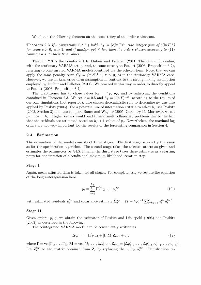
DGP I: The process is taken from the Monte Carlo study in Yap and Reinsel (1995) andis a trivariate ARMA(1,1) model with cointegrating rank, r = 2, ∆yt = Πyt−1 +ut+M1ut−1,where the initial values are set equal to zero, the errors are i.i.d. N(0,Σ) and the parameter

9

matrices are

αβ′ =

−.398 .433.121 −.340.103 .166

(1 0 −.800 1 −.48

), M1 = −

−0.7 .0 .0.3 −0.5 .0−.2 .1 .1

Σu =

1.0 .5 .4.5 1.0 .7.4 .7 1.0

. (21)

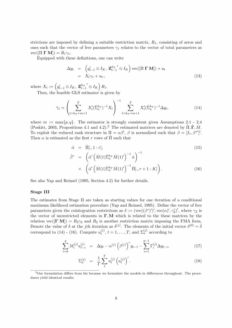
DGP II: The process is taken from Lutkepohl and Claessen (1997) that estimated aVARMA with Kronecker indices p = (2, 1, 1, 1) on US macroeconomic data.3 The initialvalues are set to zero. Thus, the process is given by A0∆yt−1 = αβ′yt−1 + Γ1∆yt−1 +A0ut−1 +M1ut−1 +M2ut−2, where αβ′ := A1 +A2 −A0 and

A0 =

1 0 0 0

−0.173 1 0 0−0.350 0 1 00.205 0 0 1

, Γ1 =

0.497 0.123 −0.548 −0.679

0 0 0 00 0 0 00 0 0 0

,

M1 =

−0.268 0 0 00.143 0.035 0.490 −0.3730.115 0.164 0.550 −0.4420.168 0.094 0.208 −0.810

, M2 =

0.151 0.112 0.104 0.464

0 0 0 00 0 0 00 0 0 0

,

Σu = 10−4 ×

0.699 0.076 −0.100 −0.4010.075 0.872 0.258 0.215−0.100 0.258 0.721 0.333−0.401 0.215 0.333 0.790

, α =

0.0130.028

0.000090.0046

, β =

1

−0.343−16.7219.35

.

(22)

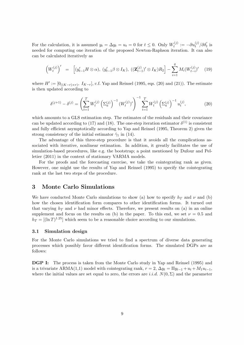
DGP III: The parameter values of the trivariate VARMA(1,1) model in FMA form aretaken from the estimation results for an interest rate systems with maturities (3M, 1Y, 10Y ).This is one of the systems considered in the forecasting study of Section 4. The initial valuesare set to the actually observed values. The process is ∆yt = Πyt−1 + ut +M1ut−1 with

Π =

−0.30 0.310 −0.02

0.14 −0.13

(1 0 −1.040 1 −1.14

), M1 =

0.35 0 00 0.35 00 0 0.35

,

Σu =

0.16 0.14 0.060.14 0.16 0.080.06 0.08 0.07

. (23)

We consider sample sizes of T = 50, 100, 200. The results on T = 200 are reported in theonline supplement. All simulations are based on R = 1000 replications.

Since different identification forms lead to different parameters, we cannot compare esti-mation accuracy. Instead, we compare the accuracy of the implied impulse response estima-

3We slightly modified their estimated model by omitting the intercept term such that the generated pro-cesses satisfy our assumptions.

10

tors. Given the moving-average representation of yt

yt = mt +t+m−1∑i=0

Φiut−i, (24)

where mt contains the influence of the initial values, let φh = vec(Φh) denote the vector ofresponses of the system to shocks h periods ago. Accuracy is here measured for each horizonas the sum of squared errors of the components R−1

∑Ri=1(φh − φh,i)′(φh − φh,i), where φh,i

is the estimated response and the dependence on an estimation and specification strategy isomitted.

We also assess the forecasting precision of the methods. We compute the traces of theestimated mean squared forecast error matrices. These are estimated for horizon h by

tr

(1

R

R∑i=1

(yT+h,i − yT+h|T,i)(yT+h,i − yT+h|T,i)′

), (25)

where yT+h,n is the value of yt at T + h for the nth replication and yT+h|T,n denotes thecorresponding h-step ahead forecast at origin T . The dependence on the specific algorithmis again suppressed. The residuals ut are used to compute forecasts recursively according to

yT+h|T = A−10

p∑j=1

Aj yT+h−j|T +

q∑j=h

Mj uT+h−j

, (26)

for h = 1, . . . , q. For h > q, the forecast is simply yT+h|T = A−10

∑pj=1Aj yT+h−j|T .

3.2 Comparison to cointegrated Echelon VARMA models

There are basically two alternative identification methods: the scalar component methodology(SCM) (Tiao and Tsay, 1989; Athanasopoulos and Vahid, 2008) and the identification via a(reverse) echelon form as proposed by Lutkepohl and Claessen (1997) for cointegrated timeseries. Unfortunately, the SCM method cannot be automatized and thus is not comparable ina large scale simulation study, see Athanasopoulos, Poskitt and Vahid (2012). We thereforecompare the FMA form only to the echelon representation. The identification via a reversedechelon representation is more complex than the FMA method in that it requires the deter-mination of K integer parameters, the so-called Kronecker indices. In line with the rest ofthe paper we focus on co-integrated processes.

While the cointegrating rank is assumed to be known, all other specification choices aremade data-dependent - in particular we consider the two specification strategies proposedin Poskitt and Lutkepohl (1995) and Poskitt (2003) for the echelon form. They are labeledPL1 and PL2 and determine the Kronecker indices equation by equation by using a selectioncriterion of the form

∆k,T (n) = log σ2k,T (n) + CTn/T, (27)

where n is the Kronecker index for equation k, σ2k,T (n) is the estimated variance of the

corresponding error term and CT is a penalty term. Since the description of these methodswould be too long for the current paper, we recommend Bartel and Lutkepohl (1998) for

11

a concise description. Poskitt and Lutkepohl (1995) proof that both procedures lead toconsistent estimators of the true Kronecker indices, provided the penalty term is chosensuitably.

All parameters of the specification methods for the echelon form described above arechosen according to a Monte Carlo study made by Bartel and Lutkepohl (1998). In particular,we have hT = max{[lnT ], pAIC , 4}, PT = [hT /2] and CT = h2

T and pAIC is determined bysearching up to a maximum order of 1.5 · (log T ). These choices are optimized for the echelonform. For the FMA form, we stick to hT = [(lnT )1.25] and ν = 0.5

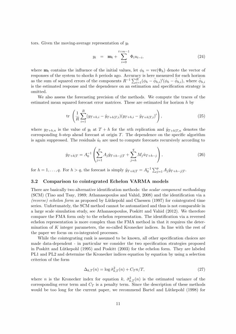
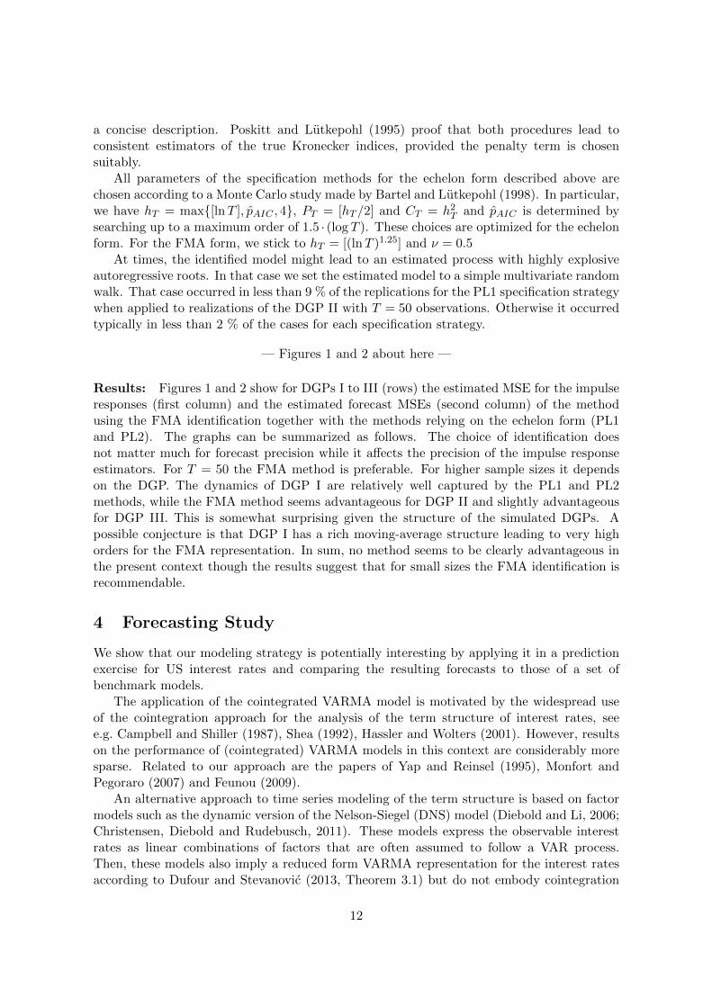
At times, the identified model might lead to an estimated process with highly explosiveautoregressive roots. In that case we set the estimated model to a simple multivariate randomwalk. That case occurred in less than 9 % of the replications for the PL1 specification strategywhen applied to realizations of the DGP II with T = 50 observations. Otherwise it occurredtypically in less than 2 % of the cases for each specification strategy.

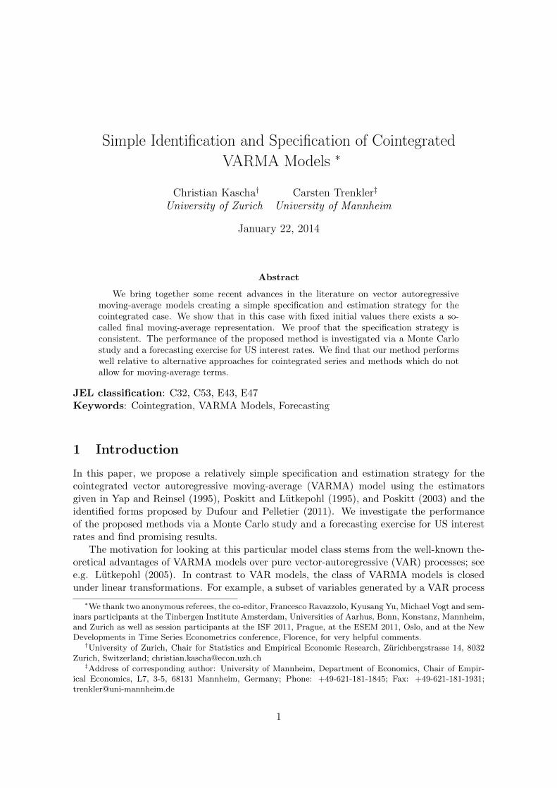
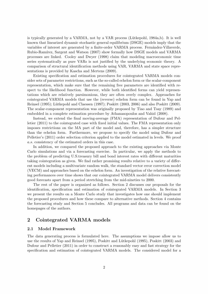
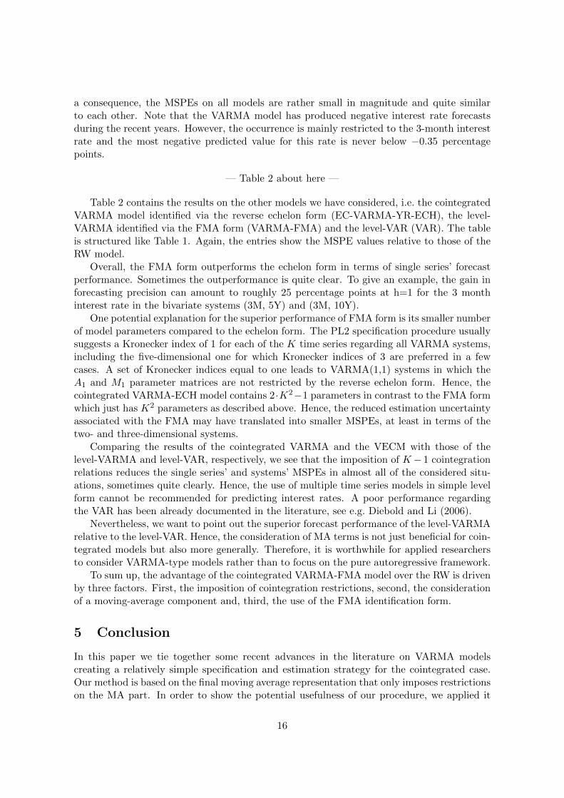
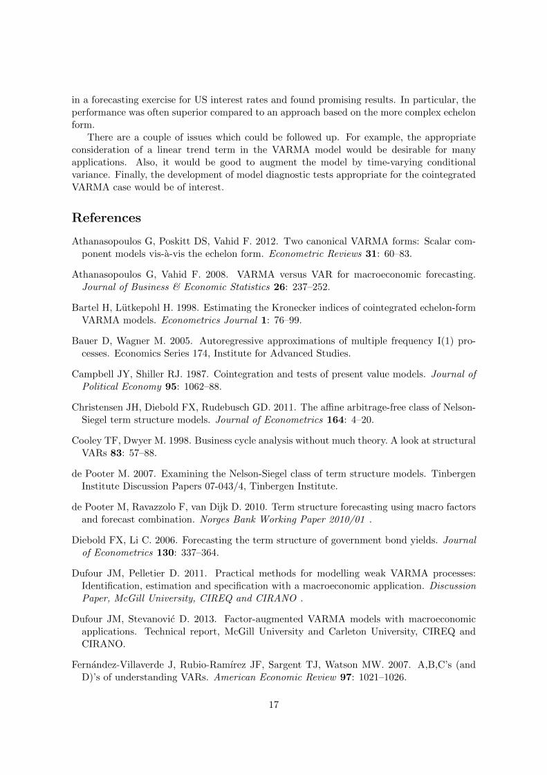
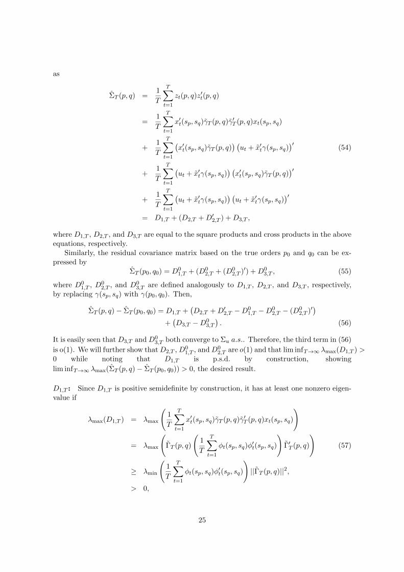
— Figures 1 and 2 about here —

Results: Figures 1 and 2 show for DGPs I to III (rows) the estimated MSE for the impulseresponses (first column) and the estimated forecast MSEs (second column) of the methodusing the FMA identification together with the methods relying on the echelon form (PL1and PL2). The graphs can be summarized as follows. The choice of identification doesnot matter much for forecast precision while it affects the precision of the impulse responseestimators. For T = 50 the FMA method is preferable. For higher sample sizes it dependson the DGP. The dynamics of DGP I are relatively well captured by the PL1 and PL2methods, while the FMA method seems advantageous for DGP II and slightly advantageousfor DGP III. This is somewhat surprising given the structure of the simulated DGPs. Apossible conjecture is that DGP I has a rich moving-average structure leading to very highorders for the FMA representation. In sum, no method seems to be clearly advantageous inthe present context though the results suggest that for small sizes the FMA identification isrecommendable.

4 Forecasting Study

We show that our modeling strategy is potentially interesting by applying it in a predictionexercise for US interest rates and comparing the resulting forecasts to those of a set ofbenchmark models.

The application of the cointegrated VARMA model is motivated by the widespread useof the cointegration approach for the analysis of the term structure of interest rates, seee.g. Campbell and Shiller (1987), Shea (1992), Hassler and Wolters (2001). However, resultson the performance of (cointegrated) VARMA models in this context are considerably moresparse. Related to our approach are the papers of Yap and Reinsel (1995), Monfort andPegoraro (2007) and Feunou (2009).

An alternative approach to time series modeling of the term structure is based on factormodels such as the dynamic version of the Nelson-Siegel (DNS) model (Diebold and Li, 2006;Christensen, Diebold and Rudebusch, 2011). These models express the observable interestrates as linear combinations of factors that are often assumed to follow a VAR process.Then, these models also imply a reduced form VARMA representation for the interest ratesaccording to Dufour and Stevanovic (2013, Theorem 3.1) but do not embody cointegration

12

restrictions. We do not consider factor models because they would require zero-coupon yielddata, like e.g. the Fama-Bliss data which only run until 2003. Furthermore, the forecastingperformance of the DNS model was inferior to that of the cointegrated VARMA models onthat Fama-Bliss data set.

4.1 Design of Forecast Comparison

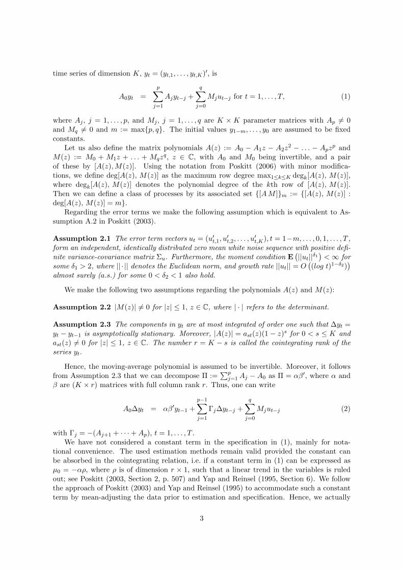
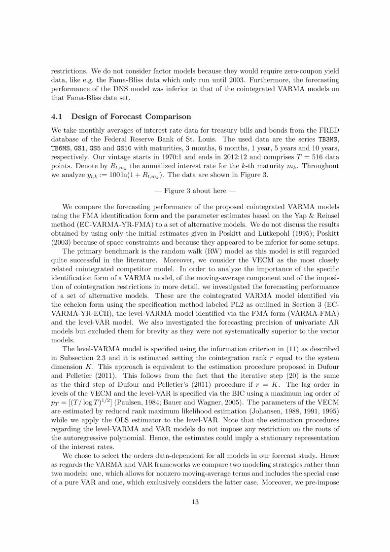
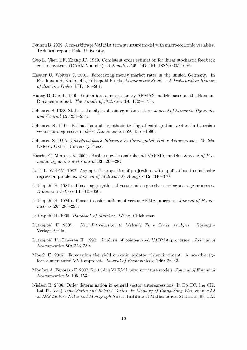
We take monthly averages of interest rate data for treasury bills and bonds from the FREDdatabase of the Federal Reserve Bank of St. Louis. The used data are the series TB3MS,TB6MS, GS1, GS5 and GS10 with maturities, 3 months, 6 months, 1 year, 5 years and 10 years,respectively. Our vintage starts in 1970:1 and ends in 2012:12 and comprises T = 516 datapoints. Denote by Rt,mk

the annualized interest rate for the k-th maturity mk. Throughoutwe analyze yt,k := 100 ln(1 +Rt,mk

). The data are shown in Figure 3.

— Figure 3 about here —

We compare the forecasting performance of the proposed cointegrated VARMA modelsusing the FMA identification form and the parameter estimates based on the Yap & Reinselmethod (EC-VARMA-YR-FMA) to a set of alternative models. We do not discuss the resultsobtained by using only the initial estimates given in Poskitt and Lutkepohl (1995); Poskitt(2003) because of space constraints and because they appeared to be inferior for some setups.

The primary benchmark is the random walk (RW) model as this model is still regardedquite successful in the literature. Moreover, we consider the VECM as the most closelyrelated cointegrated competitor model. In order to analyze the importance of the specificidentification form of a VARMA model, of the moving-average component and of the imposi-tion of cointegration restrictions in more detail, we investigated the forecasting performanceof a set of alternative models. These are the cointegrated VARMA model identified viathe echelon form using the specification method labeled PL2 as outlined in Section 3 (EC-VARMA-YR-ECH), the level-VARMA model identified via the FMA form (VARMA-FMA)and the level-VAR model. We also investigated the forecasting precision of univariate ARmodels but excluded them for brevity as they were not systematically superior to the vectormodels.

The level-VARMA model is specified using the information criterion in (11) as describedin Subsection 2.3 and it is estimated setting the cointegration rank r equal to the systemdimension K. This approach is equivalent to the estimation procedure proposed in Dufourand Pelletier (2011). This follows from the fact that the iterative step (20) is the sameas the third step of Dufour and Pelletier’s (2011) procedure if r = K. The lag order inlevels of the VECM and the level-VAR is specified via the BIC using a maximum lag order ofpT = [(T/ log T )1/2] (Paulsen, 1984; Bauer and Wagner, 2005). The parameters of the VECMare estimated by reduced rank maximum likelihood estimation (Johansen, 1988, 1991, 1995)while we apply the OLS estimator to the level-VAR. Note that the estimation proceduresregarding the level-VARMA and VAR models do not impose any restriction on the roots ofthe autoregressive polynomial. Hence, the estimates could imply a stationary representationof the interest rates.

We chose to select the orders data-dependent for all models in our forecast study. Henceas regards the VARMA and VAR frameworks we compare two modeling strategies rather thantwo models: one, which allows for nonzero moving-average terms and includes the special caseof a pure VAR and one, which exclusively considers the latter case. Moreover, we pre-impose

13

a cointegration rank of K−1 on the cointegrated VARMA and vector error correction (VEC)models.

All models are specified and estimated using the data that is available at the forecastorigin. Then, forecasts for horizon h are obtained iteratively. The considered forecast horizonsare 1, 3, 6 and 12 months. As the sample expands, all models are re-specified and re-estimated,forecasts are formed and so on - until the end of the available sample is reached. In order tohave sufficient observations for estimation, the first forecasts are obtained at Ts = 200.

Given estimates of the parameters and innovations, forecasts based on the cointegratedVARMA models are obtained by using the implied VARMA form in levels. Finally, thesample mean, which was subtracted earlier, is added to the forecasts. The latter is also donewith respect to the level-VARMA model. The point forecasts based on the RW and the VARare obtained in a standard way. Similar to the VARMA setup the estimated implied VARform is used for the VECM to obtain the forecast.

The forecast precision at a certain forecast horizon in terms of an individual series ismeasured by the (estimated) mean squared prediction errors (MSPEs). The MSPE is definedin a standard way. In the online supplement to this paper we present and discuss the jointforecasting precision, i.e. the forecasting precision with respect to a whole multiple interestrate system. To get a complete picture of the performance of the cointegrated VARMAmodels vis-a-vis the RW for h-step-ahead forecasts for the k-th series in the system wecompute cumulative sums of squared prediction errors defined as

t∑s=T s+h

e2s,RW,k,h − e2

s,M,k,h, t = T s + h, . . . , T, (28)

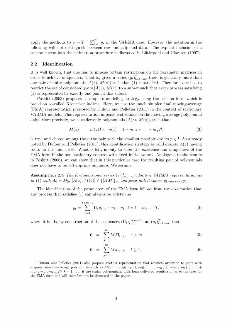
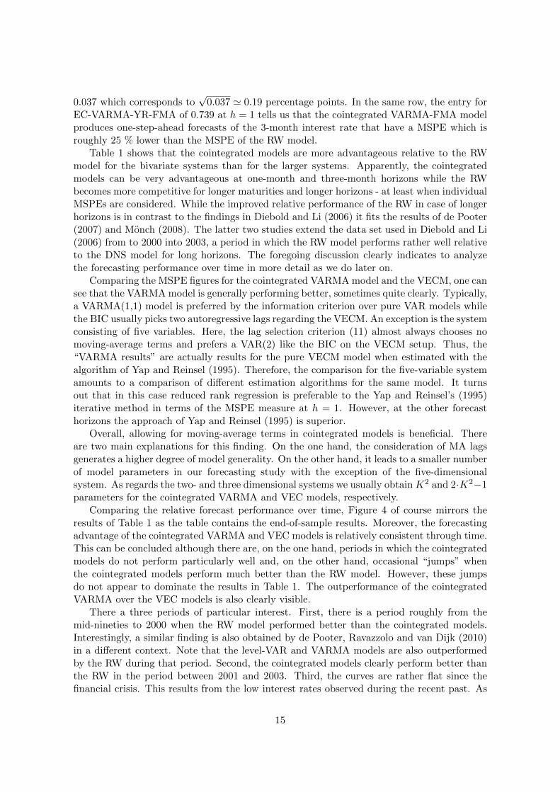
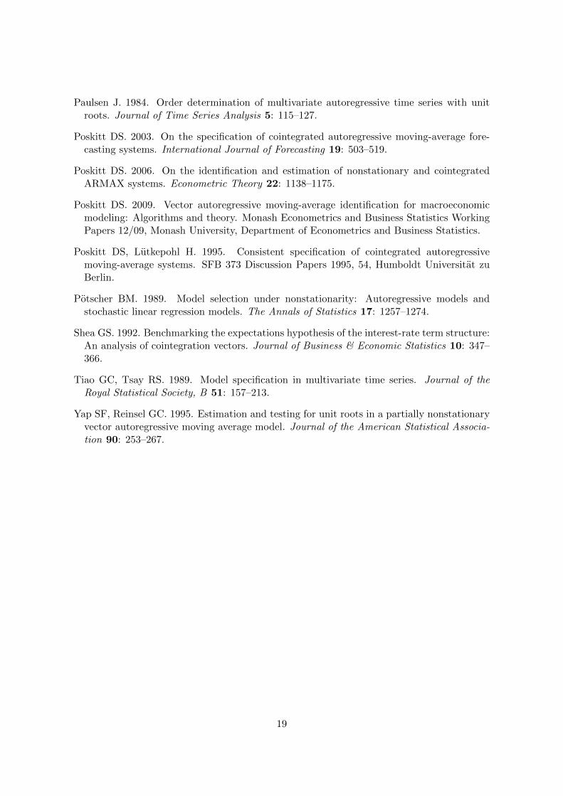
where M stands for the corresponding model and et,RW,k,h, et,M,k,h are the forecast errorsfrom predicting yt,k based on information up to t−h, i.e. et,M,k,h = yt,k− yt,k|t−h,M. Ideally,we should see that the above sum steadily increases over time if forecasting method Mis indeed preferable to the RW. We show the results for the cointegrated VARMA model inFMA form and the VECM for the system with maturities of 3 months and 1 year and forecasthorizons h = 1, 6, 12 in Figure 4. Similar conclusions can be drawn from pictures regardingthe other interest rate systems and model approaches.

4.2 Detailed Results

We have considered all bivariate and three-dimensional models that can be built from the fiveinterest rates as well as the full five-dimensional system. We provide representative findingsfor some of the interest rate systems in Tables 1 and 2.

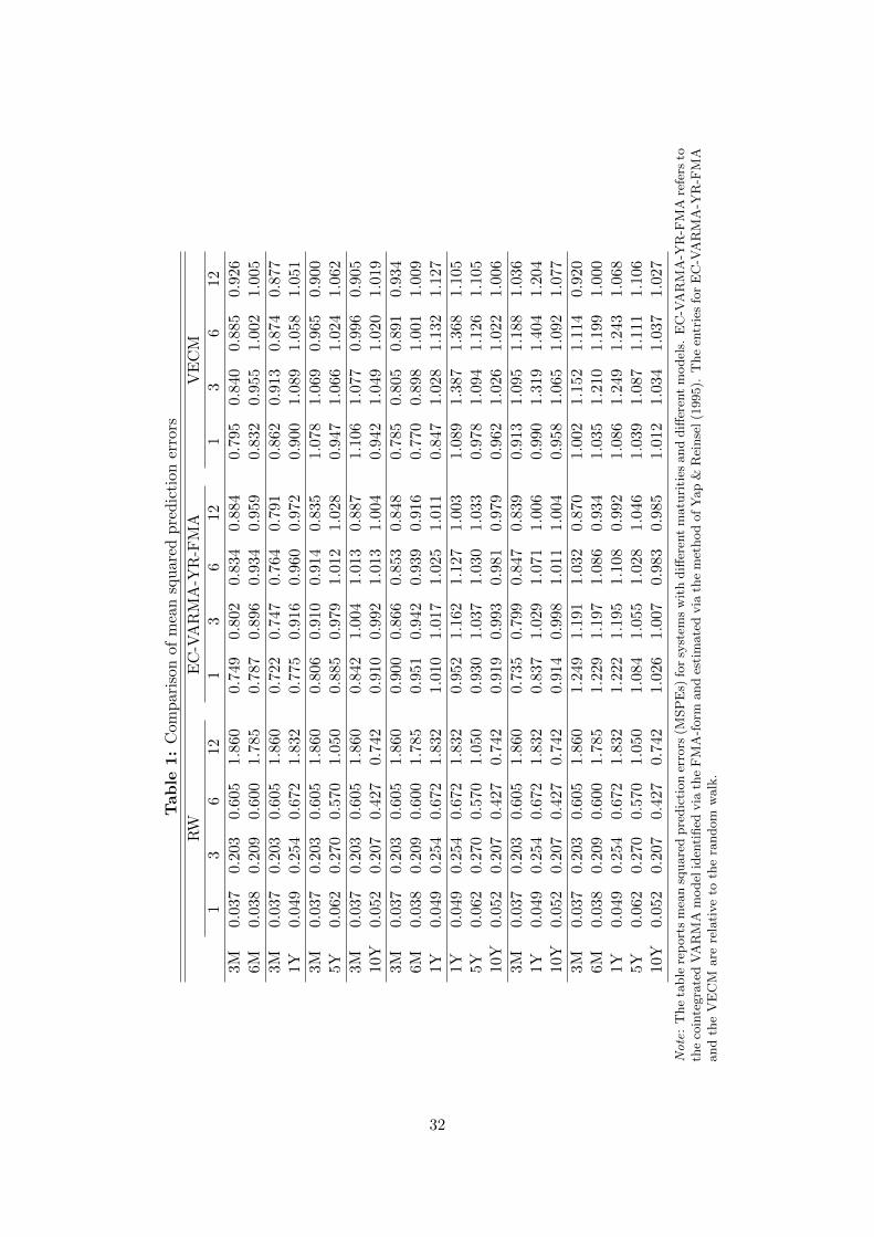
— Table 1 about here —

Table 1 contains the main results for the RW model, the cointegrated VARMA and theVECM. The table displays the MSPEs series by series for different systems and horizons.On the left column the maturities of the systems are stated; e.g. the first two rows standfor the bivariate system with interest rates for maturities 3 and 6 months. The MSPEs onthe four considered forecast horizons are given in the respective columns labeled as 1, 3, 6,and 12. The entries for the RW model are absolute while the entries for the other modelsare always relative to the corresponding entry for the RW model. For example, the firstentry in the first row tells us that the random walk produces a one-step-ahead MSPE of

14

0.037 which corresponds to√

0.037 ' 0.19 percentage points. In the same row, the entry forEC-VARMA-YR-FMA of 0.739 at h = 1 tells us that the cointegrated VARMA-FMA modelproduces one-step-ahead forecasts of the 3-month interest rate that have a MSPE which isroughly 25 % lower than the MSPE of the RW model.

Table 1 shows that the cointegrated models are more advantageous relative to the RWmodel for the bivariate systems than for the larger systems. Apparently, the cointegratedmodels can be very advantageous at one-month and three-month horizons while the RWbecomes more competitive for longer maturities and longer horizons - at least when individualMSPEs are considered. While the improved relative performance of the RW in case of longerhorizons is in contrast to the findings in Diebold and Li (2006) it fits the results of de Pooter(2007) and Monch (2008). The latter two studies extend the data set used in Diebold and Li(2006) from to 2000 into 2003, a period in which the RW model performs rather well relativeto the DNS model for long horizons. The foregoing discussion clearly indicates to analyzethe forecasting performance over time in more detail as we do later on.

Comparing the MSPE figures for the cointegrated VARMA model and the VECM, one cansee that the VARMA model is generally performing better, sometimes quite clearly. Typically,a VARMA(1,1) model is preferred by the information criterion over pure VAR models whilethe BIC usually picks two autoregressive lags regarding the VECM. An exception is the systemconsisting of five variables. Here, the lag selection criterion (11) almost always chooses nomoving-average terms and prefers a VAR(2) like the BIC on the VECM setup. Thus, the“VARMA results” are actually results for the pure VECM model when estimated with thealgorithm of Yap and Reinsel (1995). Therefore, the comparison for the five-variable systemamounts to a comparison of different estimation algorithms for the same model. It turnsout that in this case reduced rank regression is preferable to the Yap and Reinsel’s (1995)iterative method in terms of the MSPE measure at h = 1. However, at the other forecasthorizons the approach of Yap and Reinsel (1995) is superior.

Overall, allowing for moving-average terms in cointegrated models is beneficial. Thereare two main explanations for this finding. On the one hand, the consideration of MA lagsgenerates a higher degree of model generality. On the other hand, it leads to a smaller numberof model parameters in our forecasting study with the exception of the five-dimensionalsystem. As regards the two- and three dimensional systems we usually obtain K2 and 2·K2−1parameters for the cointegrated VARMA and VEC models, respectively.

Comparing the relative forecast performance over time, Figure 4 of course mirrors theresults of Table 1 as the table contains the end-of-sample results. Moreover, the forecastingadvantage of the cointegrated VARMA and VEC models is relatively consistent through time.This can be concluded although there are, on the one hand, periods in which the cointegratedmodels do not perform particularly well and, on the other hand, occasional “jumps” whenthe cointegrated models perform much better than the RW model. However, these jumpsdo not appear to dominate the results in Table 1. The outperformance of the cointegratedVARMA over the VEC models is also clearly visible.

There a three periods of particular interest. First, there is a period roughly from themid-nineties to 2000 when the RW model performed better than the cointegrated models.Interestingly, a similar finding is also obtained by de Pooter, Ravazzolo and van Dijk (2010)in a different context. Note that the level-VAR and VARMA models are also outperformedby the RW during that period. Second, the cointegrated models clearly perform better thanthe RW in the period between 2001 and 2003. Third, the curves are rather flat since thefinancial crisis. This results from the low interest rates observed during the recent past. As

15

a consequence, the MSPEs on all models are rather small in magnitude and quite similarto each other. Note that the VARMA model has produced negative interest rate forecastsduring the recent years. However, the occurrence is mainly restricted to the 3-month interestrate and the most negative predicted value for this rate is never below −0.35 percentagepoints.

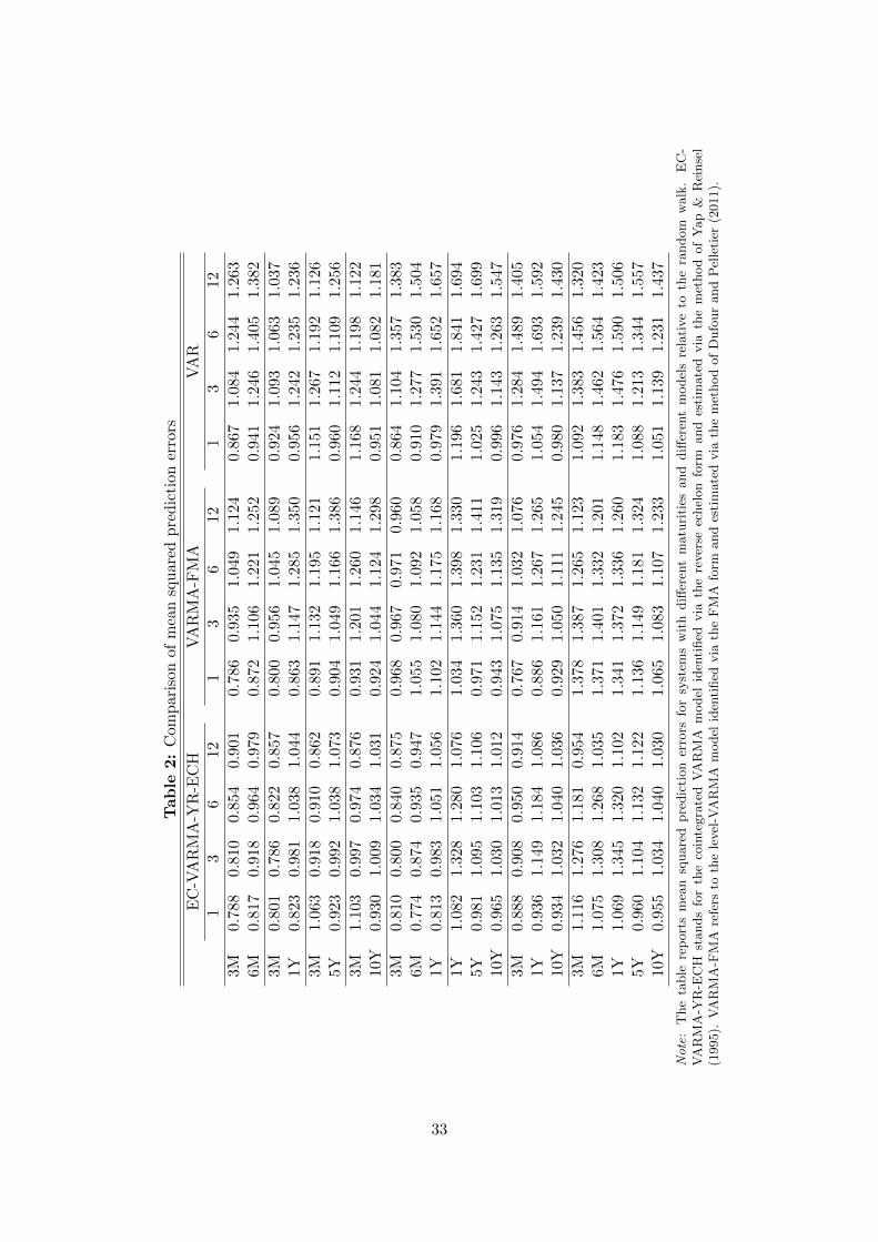
— Table 2 about here —

Table 2 contains the results on the other models we have considered, i.e. the cointegratedVARMA model identified via the reverse echelon form (EC-VARMA-YR-ECH), the level-VARMA identified via the FMA form (VARMA-FMA) and the level-VAR (VAR). The tableis structured like Table 1. Again, the entries show the MSPE values relative to those of theRW model.

Overall, the FMA form outperforms the echelon form in terms of single series’ forecastperformance. Sometimes the outperformance is quite clear. To give an example, the gain inforecasting precision can amount to roughly 25 percentage points at h=1 for the 3 monthinterest rate in the bivariate systems (3M, 5Y) and (3M, 10Y).

One potential explanation for the superior performance of FMA form is its smaller numberof model parameters compared to the echelon form. The PL2 specification procedure usuallysuggests a Kronecker index of 1 for each of the K time series regarding all VARMA systems,including the five-dimensional one for which Kronecker indices of 3 are preferred in a fewcases. A set of Kronecker indices equal to one leads to VARMA(1,1) systems in which theA1 and M1 parameter matrices are not restricted by the reverse echelon form. Hence, thecointegrated VARMA-ECH model contains 2·K2−1 parameters in contrast to the FMA formwhich just has K2 parameters as described above. Hence, the reduced estimation uncertaintyassociated with the FMA may have translated into smaller MSPEs, at least in terms of thetwo- and three-dimensional systems.

Comparing the results of the cointegrated VARMA and the VECM with those of thelevel-VARMA and level-VAR, respectively, we see that the imposition of K − 1 cointegrationrelations reduces the single series’ and systems’ MSPEs in almost all of the considered situ-ations, sometimes quite clearly. Hence, the use of multiple time series models in simple levelform cannot be recommended for predicting interest rates. A poor performance regardingthe VAR has been already documented in the literature, see e.g. Diebold and Li (2006).

Nevertheless, we want to point out the superior forecast performance of the level-VARMArelative to the level-VAR. Hence, the consideration of MA terms is not just beneficial for coin-tegrated models but also more generally. Therefore, it is worthwhile for applied researchersto consider VARMA-type models rather than to focus on the pure autoregressive framework.

To sum up, the advantage of the cointegrated VARMA-FMA model over the RW is drivenby three factors. First, the imposition of cointegration restrictions, second, the considerationof a moving-average component and, third, the use of the FMA identification form.

5 Conclusion

In this paper we tie together some recent advances in the literature on VARMA modelscreating a relatively simple specification and estimation strategy for the cointegrated case.Our method is based on the final moving average representation that only imposes restrictionson the MA part. In order to show the potential usefulness of our procedure, we applied it

16

in a forecasting exercise for US interest rates and found promising results. In particular, theperformance was often superior compared to an approach based on the more complex echelonform.

There are a couple of issues which could be followed up. For example, the appropriateconsideration of a linear trend term in the VARMA model would be desirable for manyapplications. Also, it would be good to augment the model by time-varying conditionalvariance. Finally, the development of model diagnostic tests appropriate for the cointegratedVARMA case would be of interest.

References

Athanasopoulos G, Poskitt DS, Vahid F. 2012. Two canonical VARMA forms: Scalar com-ponent models vis-a-vis the echelon form. Econometric Reviews 31: 60–83.

Athanasopoulos G, Vahid F. 2008. VARMA versus VAR for macroeconomic forecasting.Journal of Business & Economic Statistics 26: 237–252.

Bartel H, Lutkepohl H. 1998. Estimating the Kronecker indices of cointegrated echelon-formVARMA models. Econometrics Journal 1: 76–99.

Bauer D, Wagner M. 2005. Autoregressive approximations of multiple frequency I(1) pro-cesses. Economics Series 174, Institute for Advanced Studies.

Campbell JY, Shiller RJ. 1987. Cointegration and tests of present value models. Journal ofPolitical Economy 95: 1062–88.

Christensen JH, Diebold FX, Rudebusch GD. 2011. The affine arbitrage-free class of Nelson-Siegel term structure models. Journal of Econometrics 164: 4–20.

Cooley TF, Dwyer M. 1998. Business cycle analysis without much theory. A look at structuralVARs 83: 57–88.

de Pooter M. 2007. Examining the Nelson-Siegel class of term structure models. TinbergenInstitute Discussion Papers 07-043/4, Tinbergen Institute.

de Pooter M, Ravazzolo F, van Dijk D. 2010. Term structure forecasting using macro factorsand forecast combination. Norges Bank Working Paper 2010/01 .

Diebold FX, Li C. 2006. Forecasting the term structure of government bond yields. Journalof Econometrics 130: 337–364.

Dufour JM, Pelletier D. 2011. Practical methods for modelling weak VARMA processes:Identification, estimation and specification with a macroeconomic application. DiscussionPaper, McGill University, CIREQ and CIRANO .

Dufour JM, Stevanovic D. 2013. Factor-augmented VARMA models with macroeconomicapplications. Technical report, McGill University and Carleton University, CIREQ andCIRANO.

Fernandez-Villaverde J, Rubio-Ramırez JF, Sargent TJ, Watson MW. 2007. A,B,C’s (andD)’s of understanding VARs. American Economic Review 97: 1021–1026.

17

Feunou B. 2009. A no-arbitrage VARMA term structure model with macroeconomic variables.Technical report, Duke University.

Guo L, Chen HF, Zhang JF. 1989. Consistent order estimation for linear stochastic feedbackcontrol systems (CARMA model). Automatica 25: 147–151. ISSN 0005-1098.

Hassler U, Wolters J. 2001. Forecasting money market rates in the unified Germany. InFriedmann R, Knuppel L, Lutkepohl H (eds) Econometric Studies: A Festschrift in Honourof Joachim Frohn. LIT, 185–201.

Huang D, Guo L. 1990. Estimation of nonstationary ARMAX models based on the Hannan-Rissanen method. The Annals of Statistics 18: 1729–1756.

Johansen S. 1988. Statistical analysis of cointegration vectors. Journal of Economic Dynamicsand Control 12: 231–254.

Johansen S. 1991. Estimation and hypothesis testing of cointegration vectors in Gaussianvector autoregressive models. Econometrica 59: 1551–1580.

Johansen S. 1995. Likelihood-based Inference in Cointegrated Vector Autoregressive Models.Oxford: Oxford University Press.

Kascha C, Mertens K. 2009. Business cycle analysis and VARMA models. Journal of Eco-nomic Dynamics and Control 33: 267–282.

Lai TL, Wei CZ. 1982. Asymptotic properties of projections with applications to stochasticregression problems. Journal of Multivariate Analysis 12: 346–370.

Lutkepohl H. 1984a. Linear aggregation of vector autoregressive moving average processes.Economics Letters 14: 345–350.

Lutkepohl H. 1984b. Linear transformations of vector ARMA processes. Journal of Econo-metrics 26: 283–293.

Lutkepohl H. 1996. Handbook of Matrices. Wiley: Chichester.

Lutkepohl H. 2005. New Introduction to Multiple Time Series Analysis. Springer-Verlag: Berlin.

Lutkepohl H, Claessen H. 1997. Analysis of cointegrated VARMA processes. Journal ofEconometrics 80: 223–239.

Monch E. 2008. Forecasting the yield curve in a data-rich environment: A no-arbitragefactor-augmented VAR approach. Journal of Econometrics 146: 26–43.

Monfort A, Pegoraro F. 2007. Switching VARMA term structure models. Journal of FinancialEconometrics 5: 105–153.

Nielsen B. 2006. Order determination in general vector autoregressions. In Ho HC, Ing CK,Lai TL (eds) Time Series and Related Topics: In Memory of Ching-Zong Wei, volume 52of IMS Lecture Notes and Monograph Series. Institute of Mathematical Statistics, 93–112.

18

Paulsen J. 1984. Order determination of multivariate autoregressive time series with unitroots. Journal of Time Series Analysis 5: 115–127.

Poskitt DS. 2003. On the specification of cointegrated autoregressive moving-average fore-casting systems. International Journal of Forecasting 19: 503–519.

Poskitt DS. 2006. On the identification and estimation of nonstationary and cointegratedARMAX systems. Econometric Theory 22: 1138–1175.

Poskitt DS. 2009. Vector autoregressive moving-average identification for macroeconomicmodeling: Algorithms and theory. Monash Econometrics and Business Statistics WorkingPapers 12/09, Monash University, Department of Econometrics and Business Statistics.

Poskitt DS, Lutkepohl H. 1995. Consistent specification of cointegrated autoregressivemoving-average systems. SFB 373 Discussion Papers 1995, 54, Humboldt Universitat zuBerlin.

Potscher BM. 1989. Model selection under nonstationarity: Autoregressive models andstochastic linear regression models. The Annals of Statistics 17: 1257–1274.

Shea GS. 1992. Benchmarking the expectations hypothesis of the interest-rate term structure:An analysis of cointegration vectors. Journal of Business & Economic Statistics 10: 347–366.

Tiao GC, Tsay RS. 1989. Model specification in multivariate time series. Journal of theRoyal Statistical Society, B 51: 157–213.

Yap SF, Reinsel GC. 1995. Estimation and testing for unit roots in a partially nonstationaryvector autoregressive moving average model. Journal of the American Statistical Associa-tion 90: 253–267.

19

A Proofs

Proof of Theorem 2.1:

⇒: Suppose (yt)Tt=1−m satisfies (1) given initial conditions. One can view the sequence

(ut)Tt=1−m as a solution to (1) viewed as system of equations for the errors and given initial

conditions u0, . . . , u1−m. Then we know that (ut)Tt=1−m is the sum of a particular solution

and the appropriately chosen solution of the corresponding homogeneous system of equations,ut = uPt + (−nt), say.

Define the sequence (Πi)i∈N0 by the recursive relations Π0 = −IK and

Ai =i∑

j=0

MjΠi−j , for i = 1, . . . ,m (29)

0 =

m∑j=0

MjΠi−j , for i > m (30)

Define now (uPt )Tt=1−m by uPt := yt −∑t+m−1

s=1 Πsyt−s, where∑0

s=1 Πsyt−s := 0. Then,(uPt )Tt=1−m is indeed a particular solution as for t ≥ 1

p∑j=0

MjuPt−j =

m∑j=0

Mj

(yt−j −

t−j+m−1∑s=1

Πsyt−s−j

)

= A0yt −m∑j=1

Ajyt−j . (31)

Further, define (nt)Tt=1−m by nt = uPt − ut for t = 1−m, . . . , 0 and 0 =

∑mi=0Mint−i, for t =

1, . . . , T . Since the initial values determine the rest of the series, we also have ut = uPt − ntfor t ≥ 1.

Therefore, yt =∑t+m−1

s=1 Πsyt−s + ut + nt for t = 1−m, . . . , 0.

⇐ : Conversely, suppose (yt)Tt=1−m admits an autoregressive representation as in (4) and

there exist (K × K) matrices Mj j = 0, . . . ,m such that 0 =∑m

j=0MjΠi−j for i > m and0 =

∑mj=0Mjnt−j , for t = 1, . . . , T.. Then, for t = 1, . . . , T , it holds that

m∑j=0

Mjyt−j =

m∑j=0

Mj

t−j+m−1∑s=1

Πsyt−j−s +

m∑j=0

Mjut−j +

m∑j=0

Mjnt−j (32)

Moving all terms involving yt to the left-hand side yields

−t+m−1∑v=0

min(v,m)∑j=0

MjΠv−jyt−v = −m∑v=0

( v∑j=0

MjΠv−j)yt−v

= A0yt −m∑v=1

Avyt−v =

m∑j=0

Mjut−j (33)

where A0 := −M0Π0 = M0 and Av :=∑v

j=0MjΠv−j , v = 1, . . . ,m.

20

Proof of Theorem 2.2:

From Theorem 2.1, (yt)Tt=1−m has a autoregressive representation with the associated series

(Π)T+m−1i=0 and (nt)

Tt=1−m. One considers then the set of all polynomials, m(z) = 1 +m1z +

. . .mqzq, for which

0 =

q∑j=0

mjΠi−j (34)

0 =

q∑j=0

mjnt−j (35)

is true for i > q and t ≥ t for some t, 1 −m ≤ t ≤ T . Denote this set by S. Because of (7)and (8), we know that the (normalized) determinant, |M(z)|, satisfies the above conditionswith q = q and t = q −m+ 1. Therefore, S is not empty. Denote one solution to

minm(z)∈S

deg(m(z)), (36)

by m0(z) with degree q0 and corresponding t0, where deg : S → N is the function that assignsthe degree to every polynomial in S. Suppose, there is another solution of the same degreem1(z) = 1 +m1,1z+ . . .+m1,q0z

q0 . Since both polynomials are of degree q0, a = m0,q0/m1,q0

exists and one gets

0 =

q∑j=0

(m0,j − am1,j)Πi−j (37)

0 =

q∑j=0

(m0,j − am1,j)nt−j (38)

Then, normalization of the first non-zero coefficient of (m0(z)− am1(z)) would give a poly-nomial in S with degree smaller than q0, a contradiction. Thus m0(z) is unique.

Given m0(z), define A0,0 = IK and A0,v :=∑v

j=0m0,jΠv−j , v = 1, . . . , q0 and p0 as theminimal number such that A0,v = 0 for v > p0.

Then, condition (34) alone would imply left-coprimeness of [A0(z), m0(z)IK ] but if (nt)Tt=1−m 6=

0 the minimal orders p0, q0 might well be above those of the left-coprime solution to (34).

Proof of Theorem 2.3:

Similar to Guo, Chen and Zhang (1989), we proof (pT , qT ) → (p0, q0) a.s. by showing thatthe only limit point of (pT , qT ) is indeed (p0, q0) with probability one, where p0 and q0 arethe true lag orders. Thus, the convergence of pT and qT follows, which is equivalent to jointconvergence. In order to show this, we demonstrate that the events “(pT , qT ) has a limitpoint (p, q) with p+ q > p0 + q0 ” (assuming p ≥ p0, q ≥ q0) and “(pT , qT ) has a limit point(p, q) with p < p0 or q < q0 ” both have probability zero.

Following Huang and Guo (1990) we rely on the spectral norm in order to analyzethe convergence behaviour of various sample moments; that is, for a (m × n) matrix A,||A|| :=

√λmax(AA′), where λmax(·) denotes the maximal eigenvalue. Lutkepohl (1996, Ch.

21

8) provides a summary of the properties of this norm. The stochastic order symbols o andO are understood in the context of almost sure convergence.

Case 1: p ≥ p0, q ≥ q0, p+ q > p0 + q0

For simplicity, write T instead of N in our lag selection criterion (11). Then

DP (p, q)−DP (p0, q0) = ln[|ΣT (p, q)|/|ΣT (p0, q0)|] + c(lnT )1+v

T, (39)

where c > 0 is a constant.We have to show that DP (p, q) − DP (p0, q0) has a positive limit for any pair p, q with

p0 ≤ p ≤ pT , q0 ≤ q ≤ qT , and p + q > p0 + q0. Similar to Nielsen (2006, Proof ofTheorem 2.5), it is sufficient to show that T (ΣT (p0, q0) − ΣT (p, q)) = O{g(T )} such that(lnT )1+v/g(T )→∞ in this case.

Let us introduce the following notation:

φ0t (p, q) = [y′t, . . . , y

′t−p+1, u

′t, . . . u

′t−q+1]′

φt(p, q) = [y′t, . . . , y′t−p+1, (u

hTt )′, . . . , (uhTt−q+1)′]′

YT = [y′1, . . . , y′T ]′

UT = [u′1, . . . , u′T ]′

x0t (p, q) = [(φ0

t−1(p, q)′ ⊗ IK)R]′ (40)

xt(p, q) = [(φt−1(p, q)′ ⊗ IK)R]′

X0T (p, q) = [x0

1(p, q), . . . , x0T (p, q)]′

XT (p, q) = [x1(p, q), . . . , xT (p, q)]′

γ(p, q) = [vec(A1, A2, . . . , Ap)′,m1,m2, . . . ,mq]

′,

where γ(p, q) is the (K2 ·(p+q)×1) vector of true parameters such that Ai = 0 and mj = 0 fori > p0, j > q0, respectively, and R is implicitly defined such that vec[A1, . . . , Ap,M1, . . .Mq] =Rγ(p, q).

Then, one can write

yt =

p∑i=1

Aiyt−i + ut +

q∑i=1

Miut−i

= [A1, . . . , Ap,M1, . . .Mq]φ0t−1(p, q) + ut (41)

= (φ0t−1(p, q)′ ⊗ IK)vec[A1, . . . , Ap,M1, . . .Mq] + ut

= x0t (p, q)

′γ(p, q) + ut

in order to summarize the model in matrix notation by

YT = X0T (p, q)γ(p, q) + UT = XT (p, q)γ(p, q) +RT + UT , (42)

where

RT := [X0T (p, q)−XT (p, q)]γ(p, q). (43)

22

RT does not depend on p, q for p ≥ p0, q ≥ q0 and can be decomposed asRT = [r′0, r′1, . . . , r

′T−1]′,

where rt, t = 0, 1, . . . , T − 1, is a K × 1 vector. Let ZT (p, q) = [z1(p, q)′, . . . , zT (p, q)′]′ be theOLS residuals obtained from regressing YT on XT (p, q), i.e.

ZT (p, q) = YT −XT (p, q)[XT (p, q)′XT (p, q)

]−1XT (p, q)′YT

= [RT + UT ]−XT (p, q)[XT (p, q)′XT (p, q)

]−1XT (p, q)′[RT + UT ]. (44)

The estimator of the error covariance matrix Σu in dependence on p and q is given byΣT (p, q) = T−1

∑Tt=1 zt(p, q)zt(p, q)

′. Furthermore, note that ΣT (p0, q0)− ΣT (p, q) is positivesemidefinite since p ≥ p0 and q ≥ q0 in the current setup. Hence, we have

‖ ΣT (p0, q0)− ΣT (p, q) ‖= λmax

(ΣT (p0, q0)− ΣT (p, q)

)≤ tr

(ΣT (p0, q0)− ΣT (p, q)

)= tr

(ΣT (p0, q0)

)− tr

(ΣT (p, q)

)(45)

= T−1[RT + UT ]′XT (p, q)[XT (p, q)′XT (p, q)

]−1XT (p, q)′[RT + UT ]

− T−1[RT + UT ]′XT (p0, q0)[XT (p0, q0)′XT (p0, q0)

]−1XT (p0, q0)′[RT + UT ].

We have for the terms on the right-hand side (r.h.s.) of the last equality in (45)

[RT + UT ]′XT (p, q)[XT (p, q)′XT (p, q)

]−1XT (p, q)′[RT + UT ]

= O(||[XT (p, q)′XT (p, q)

]−1/2XT (p, q)′[RT + UT ]||2

)= O

(||[XT (p, q)′XT (p, q)

]−1/2XT (p, q)′RT ||2

)+O

(||[XT (p, q)′XT (p, q)

]−1/2XT (p, q)′UT ||2

),

(46)

where the result holds for all p ≥ p0 and q ≥ q0.As in Poskitt and Lutkepohl (1995, Proof of Theorem 3.2), we obtain from Lai and

Wei (1982, Theorem 3), with a correction mentioned in Potscher (1989, p. 1268), for anym = max(p, q)

||[XT (p, q)′XT (p, q)

]−1/2XT (p, q)′UT ||2

= O

(max

{1, ln+

(s∑

n=1

∑t

||yt−n||2 + ||uhTt−n||2)})

(47)

= O(ln m) +O

(ln

(O

{∑t

||yt||2 + ||uhTt ||2}))

,

where ln+(x) denotes the positive part of ln(x). Moreover, we have that∑

t ||yt||2 = O(T g)due to Assumption 3.3, where the growth rate is independent of m, see Poskitt and Lutkepohl(1995, Proof of Theorem 3.2, Proof of Lemma 3.1). Therefore, the second term on the r.h.s.of (47) is O(lnT ) for all m. Hence, the left-hand side (l.h.s.) of (47) is O(lnT ) sincem ≤ sT ≤ hT = [c(lnT )a], c > 0, a > 1.

Similar to Poskitt and Lutkepohl (1995, Proof of Theorem 3.2) we obtain from a standard

23

result in least squares

||[XT (p, q)′XT (p, q)

]−1/2XT (p, q)′RT ||2 ≤

T−1∑t=0

K∑i=1

r2i,t

≤ ||γ(p, q)||2 ·q∑

n=1

T∑t=1

||ut−n − uhTt−n||2 = O(lnT ), (48)

where the last line follows from Poskitt (2003, Proposition 3.1) due to Assumption 3.3, ourchoice of hT and since ||γ(p, q)|| = constant < ∞ independent of (p, q). Hence, we haveT−1[RT + UT ]′XT (p, q) [XT (p, q)′XT (p, q)]−1 ×XT (p, q)′[RT + UT ] = O(lnT/T ).

Using (46 - 48), we have ‖ ΣT (p0, q0)− ΣT (p, q) ‖= O (lnT/T ) such that T (ΣT (p0, q0)−ΣT (p, q)) = O{ln(T )}, the desired result, and therefore DP (p, q) − DP (p0, q0) > 0 a.s. forsufficiently large T .

Case 2: (p, q) with p < p0 or q < q0

For (p, q) with p < p0 or q < q0, write

DP (p, q)−DP (p0, q0) = ln |IK + (ΣT (p, q)− ΣT (p0, q0))Σ−1T (p0, q0))|+ o(1) (49)

As in Nielsen (2006, Proof of Theorem 2.4), it suffices to show that lim infT→∞ λmax(ΣT (p, q)−ΣT (p0, q0)) > 0. To do so, let us introduce some further notation:

γT (p, q) =[X ′T (p, q)XT (p, q)

]−1X ′T (p, q)YT (50)

= [vec(A1, A2, . . . , Ap)′, m1, m2, . . . , mq]

′.

and, defining sp = max(p, p0) and sq = max(q, q0),

γ0T (p, q) = [vec(A1, A2, . . . , Asp)′, m1, m2, . . . , msq ]′ (51)

with Ai = 0 for i > p and mi = 0 for i > q. Then, we get

ZT (p, q) = YT −XT (p, q)γT (p, q) = YT −XT (sp, sq)γ0T (p, q)

= UT + XTγ(sp, sq) +XT (sp, sq)γT (p, q), (52)

where γ(p, q) is defined as above in Case 1,

XT := (X0T (sp, sq)−XT (sp, sq)), (53)

and γT (p, q) = γ(sp, sq)− γ0T (p, q).

Let x′t and x′t(sp, sq) be the typical K × (pK2 + q) (sub)matrices of the TK × (pK2 + q)matrices XT and XT (sp, sq), respectively, i.e. the partition of XT and XT (sp, sq) is analogousto XT (p, q) above. Then, for p < p0 or q < q0, the residual covariance matrix can be written

24

as

ΣT (p, q) =1

T

T∑t=1

zt(p, q)z′t(p, q)

=1

T

T∑t=1

x′t(sp, sq)γT (p, q)γ′T (p, q)xt(sp, sq)

+1

T

T∑t=1

(x′t(sp, sq)γT (p, q)

) (ut + x′tγ(sp, sq)

)′(54)

+1

T

T∑t=1

(ut + x′tγ(sp, sq)

) (x′t(sp, sq)γT (p, q)

)′+

1

T

T∑t=1

(ut + x′tγ(sp, sq)

) (ut + x′tγ(sp, sq)

)′= D1,T + (D2,T +D′2,T ) +D3,T ,

where D1,T , D2,T , and D3,T are equal to the square products and cross products in the aboveequations, respectively.

Similarly, the residual covariance matrix based on the true orders p0 and q0 can be ex-pressed by

ΣT (p0, q0) = D01,T + (D0

2,T + (D02,T )′) +D0

3,T , (55)

where D01,T , D0

2,T , and D03,T are defined analogously to D1,T , D2,T , and D3,T , respectively,

by replacing γ(sp, sq) with γ(p0, q0). Then,

ΣT (p, q)− ΣT (p0, q0) = D1,T +(D2,T +D′2,T −D0

1,T −D02,T − (D0

2,T )′)

+(D3,T −D0

3,T

). (56)

It is easily seen that D3,T and D03,T both converge to Σu a.s.. Therefore, the third term in (56)

is o(1). We will further show thatD2,T , D01,T , andD0

2,T are o(1) and that lim infT→∞ λmax(D1,T ) >0 while noting that D1,T is p.s.d. by construction, showing

lim infT→∞ λmax(ΣT (p, q)− ΣT (p0, q0)) > 0, the desired result.

D1,T : Since D1,T is positive semidefinite by construction, it has at least one nonzero eigen-value if

λmax(D1,T ) = λmax

(1

T

T∑t=1

x′t(sp, sq)γT (p, q)γ′T (p, q)xt(sp, sq)

)

= λmax

(ΓT (p, q)

(1

T

T∑t=1

φt(sp, sq)φ′t(sp, sq)

)Γ′T (p, q)

)(57)

≥ λmin

(1

T

T∑t=1

φt(sp, sq)φ′t(sp, sq)

)||ΓT (p, q)||2,

> 0,

25

where ΓT (p, q) = [A1, . . . , Mq] is γ(p, q) augmented to matrix form. Then, one obtains

limT→∞ inf T−1λmin(∑T

t=1 φt(sp, sq)φ′t(sp, sq)) > 0 a.s., according to Poskitt and Lutkepohl

(1995, Proof of Theorem 3.2), and ||ΓT (p, q)||2 = constant > 0 from Huang and Guo (1990,p. 1753). This gives lim infT→∞ λmax(D1,T ) > 0.

D01,T : We have

γT (p0, q0) = γ(p0, q0)− γ0T (p0, q0) (58)

= −[X ′T (p0, q0)XT (p0, q0)

]−1X ′T (p0, q0)

[XTγ(p0, q0) + UT

]due to (42), (50), (51), and (53). Therefore,∥∥∥∥∥ 1

T

T∑t=1

x′t(p0, q0)γT (p0, q0)γT (p0, q0)′xt(p0, q0)

∥∥∥∥∥≤ 1

T

T∑t=1

||x′t(p0, q0)γT (p0, q0)γT (p0, q0)′xt(p0, q0)||

=1

T

T∑t=1

γT (p0, q0)′xt(p0, q0)x′t(p0, q0)γT (p0, q0) (59)

=1

TγT (p0, q0)′

(X ′T (p0, q0)XT (p0, q0)

)γT (p0, q0),

and, using the above result on γT ,

=1

T

[XTγ(p0, q0) + UT

]′XT (p0, q0)

[X ′T (p0, q0)XT (p0, q0)

]−1

× X ′T (p0, q0)[XTγ(p0, q0) + UT

](60)

=1

TO(lnT ),

where the last line follows from (46-48) of the first part of the proof; compare also Huangand Guo (1990, pp. 1754).

D2,T : Defining the (T × (sp + sq) ·K) matrix ΦT := [φ0(sp, sq), . . . , φT−1(sp, sq)]′ and let

UT := [u1, . . . , uT ]′, XT := [x′1γ(sp, sq), . . . , x′Tγ(sp, sq)]

′, then tedious but straightforward

26

calculations lead to∥∥∥∥∥ 1

T

T∑t=1

(x′t(sp, sq)γT (p, q))(ut + x′tγ(sp, sq))′

∥∥∥∥∥=

∥∥∥∥∥ 1

T

T∑t=1

ΓT (p, q)φt(sp, sq)(ut + x′tγ(sp, sq))′

∥∥∥∥∥=

∥∥∥∥∥ 1

TΓT (p, q)(Φ′TΦT )1/2(Φ′TΦT )−1/2

T∑t=1

φt(sp, sq)(ut + x′tγ(sp, sq))′

∥∥∥∥∥≤ 1

T||ΓT (p, q)(Φ′TΦT )1/2|| ||(Φ′TΦT )−1/2Φ′T (UT +XT )|| (61)

≤(

1

TΓT (p, q)(Φ′TΦT )Γ′T (p, q)

)1/2

×(

1

T(UT + XTγ)′(ΦT ⊗ IK)((Φ′TΦT )−1 ⊗ IK)(Φ′T ⊗ IK)(UT + XTγ)

)1/2

= [O(1)]1/2[O

(1

TlnT

)]1/2

= o(1)

following from the results on D1,T and again from (46-48) of the first part of the proof. Notein this respect that the results in (47) and (48) also hold when using the regressor matrixΦT ⊗ IK appearing in (61). This is due to the fact that the relevant properties of linearprojections and OLS do not depend on whether the restricted or unrestricted form of theregressor matrix is used.

D02,T : Similar to the arguments used for D2,T using arguments identical to those used to

evaluate D01,T , we can write∥∥∥∥∥ 1

T

T∑t=1

(x′tγT (p0, q0))(ut + x′tγ(p0, q0)

∥∥∥∥∥≤ 1

T[γT (p0, q0)′(X ′T (p0, q0)XT (p0, q0))γT (p0, q0)]1/2

× [(UT + X ′Tγ(p0, q0))′(UT + X ′Tγ(p0, q0))]1/2 (62)

=

[O

(1

TlnT

)]1/2

[O(1)]1/2 = o(1)

noting that T−1(UT + X ′Tγ(p0, q0))′(UT + X ′Tγ(p0, q0)) = T−1U ′TUT + o(1) = O(1) due to theresults of Poskitt and Lutkepohl (1995, Proof of Theorem 3.2) and applying Poskitt (2003,Proposition 3.1). This completes the proof.

27

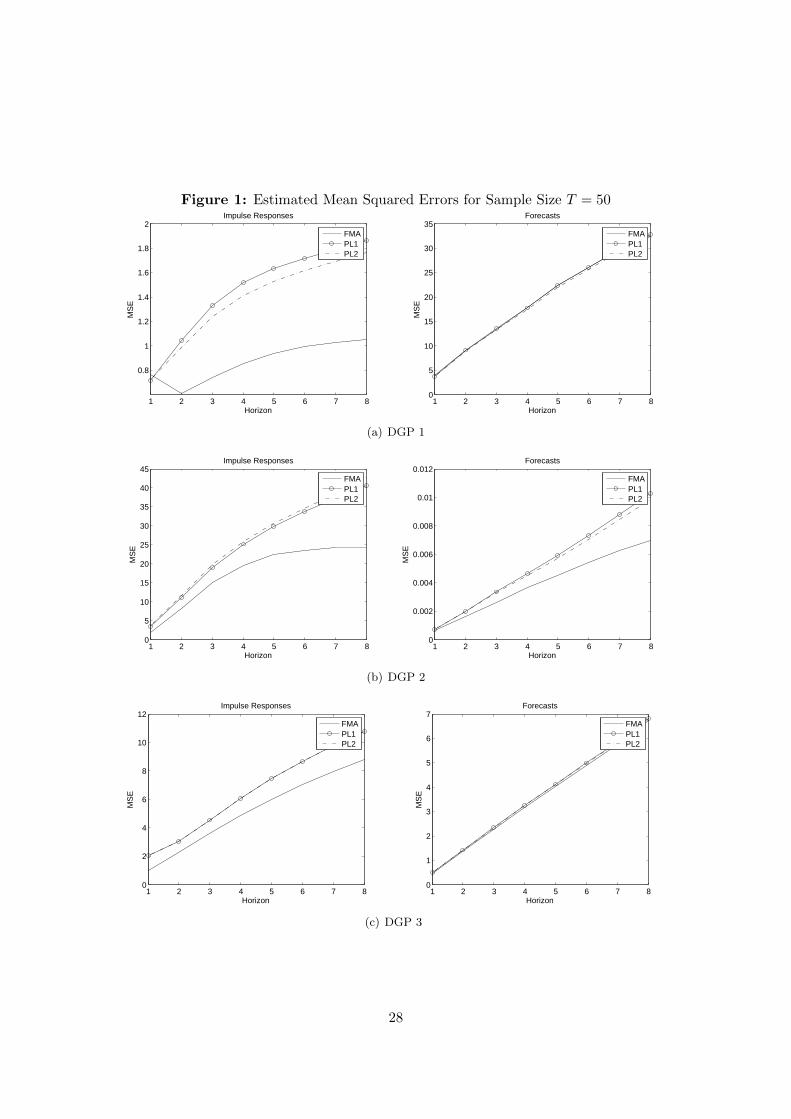
Figure 1: Estimated Mean Squared Errors for Sample Size T = 50

1 2 3 4 5 6 7 8

0.8

1

1.2

1.4

1.6

1.8

2

Horizon

MS

E

Impulse Responses

FMAPL1PL2

1 2 3 4 5 6 7 80

5

10

15

20

25

30

35

HorizonM

SE

Forecasts

FMAPL1PL2

(a) DGP 1

1 2 3 4 5 6 7 80

5

10

15

20

25

30

35

40

45

Horizon

MS

E

Impulse Responses

FMAPL1PL2

1 2 3 4 5 6 7 80

0.002

0.004

0.006

0.008

0.01

0.012

Horizon

MS

E

Forecasts

FMAPL1PL2

(b) DGP 2

1 2 3 4 5 6 7 80

2

4

6

8

10

12

Horizon

MS

E

Impulse Responses

FMAPL1PL2

1 2 3 4 5 6 7 80

1

2

3

4

5

6

7

Horizon

MS

E

Forecasts

FMAPL1PL2

(c) DGP 3

28

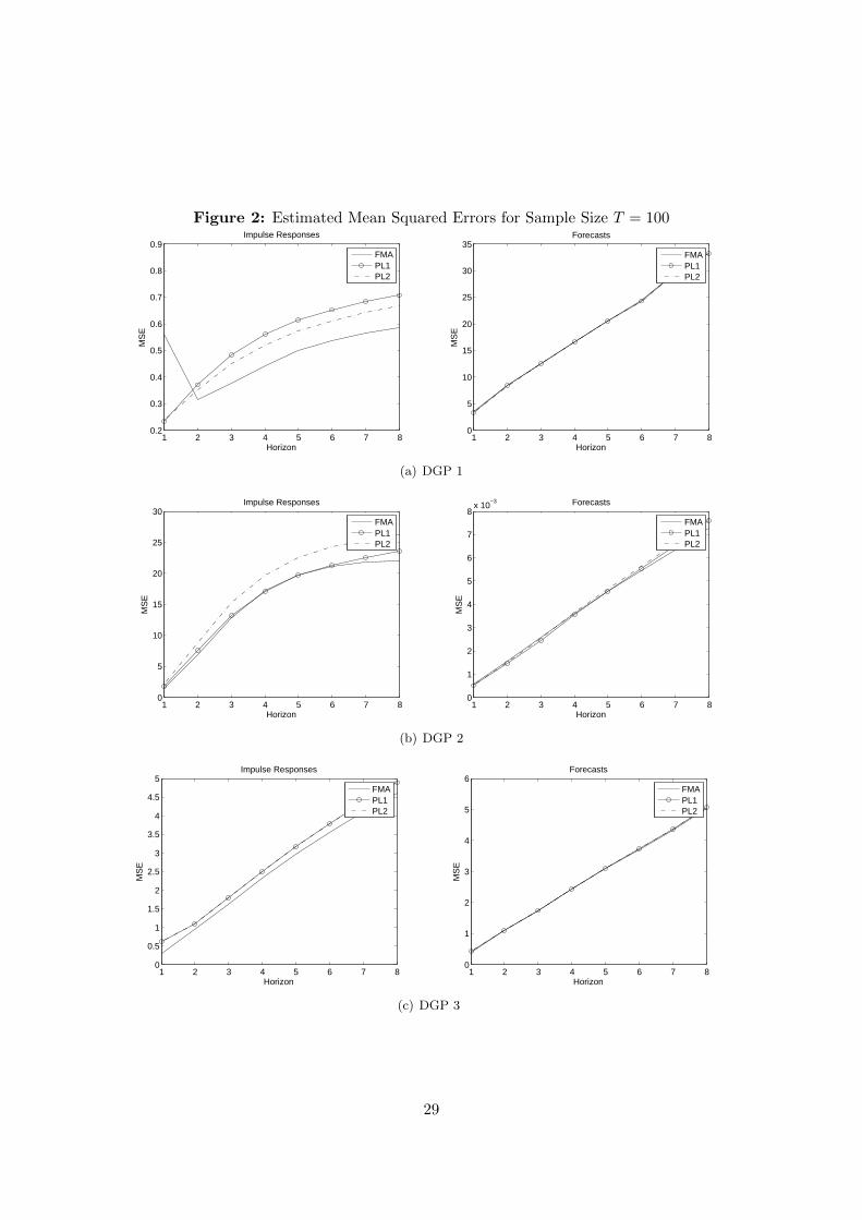
Figure 2: Estimated Mean Squared Errors for Sample Size T = 100

1 2 3 4 5 6 7 80.2

0.3

0.4

0.5

0.6

0.7

0.8

0.9

Horizon

MS

E

Impulse Responses

FMAPL1PL2

1 2 3 4 5 6 7 80

5

10

15

20

25

30

35

HorizonM

SE

Forecasts

FMAPL1PL2

(a) DGP 1

1 2 3 4 5 6 7 80

5

10

15

20

25

30

Horizon

MS

E

Impulse Responses

FMAPL1PL2

1 2 3 4 5 6 7 80

1

2

3

4

5

6

7

8x 10

−3

Horizon

MS

E

Forecasts

FMAPL1PL2

(b) DGP 2

1 2 3 4 5 6 7 80

0.5

1

1.5

2

2.5

3

3.5

4

4.5

5

Horizon

MS

E

Impulse Responses

FMAPL1PL2

1 2 3 4 5 6 7 80

1

2

3

4

5

6

Horizon

MS

E

Forecasts

FMAPL1PL2

(c) DGP 3

29

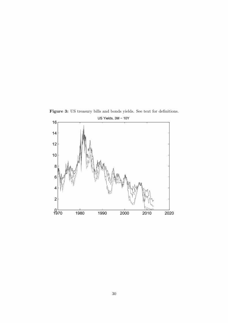
Figure 3: US treasury bills and bonds yields. See text for definitions.

30

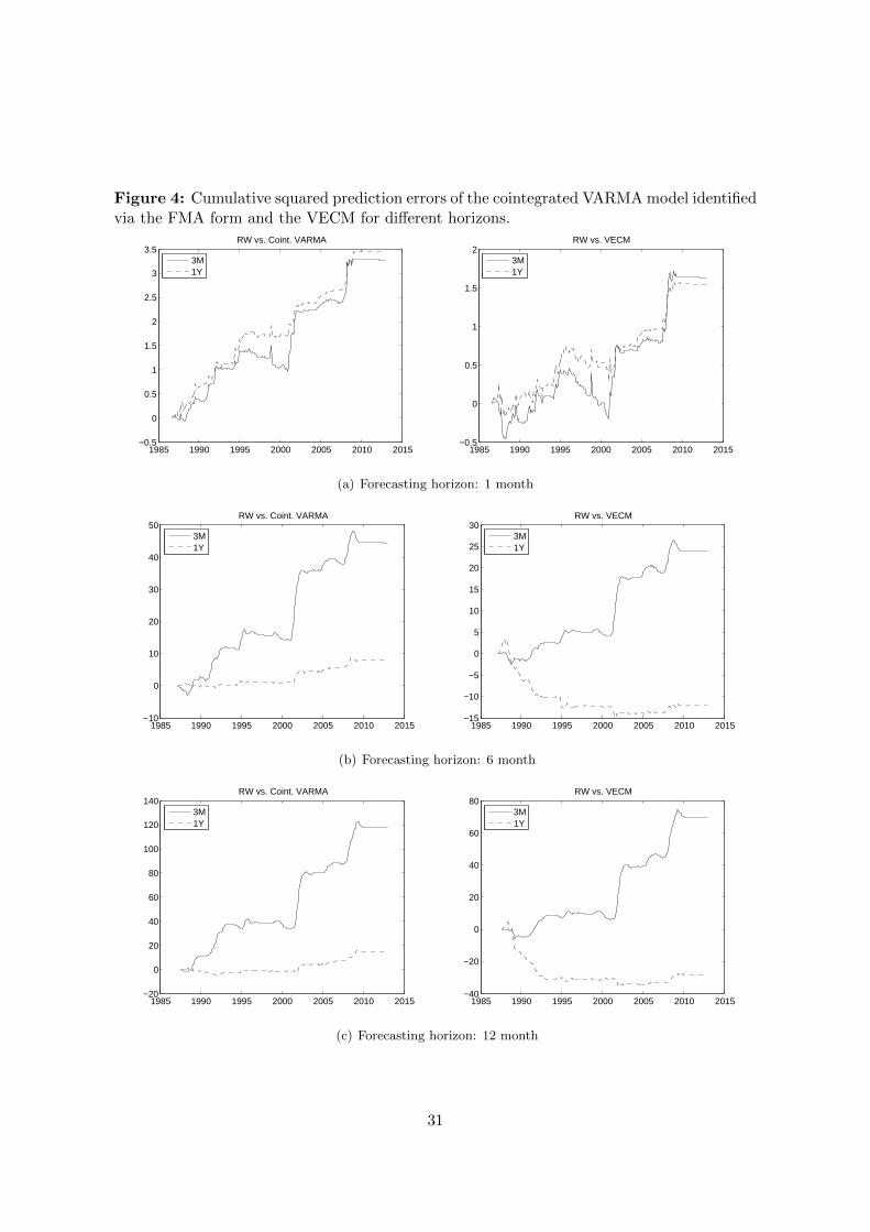
Figure 4: Cumulative squared prediction errors of the cointegrated VARMA model identifiedvia the FMA form and the VECM for different horizons.

1985 1990 1995 2000 2005 2010 2015−0.5

0

0.5

1

1.5

2

2.5

3

3.5RW vs. Coint. VARMA

3M1Y

1985 1990 1995 2000 2005 2010 2015−0.5

0

0.5

1

1.5

2RW vs. VECM

3M1Y

(a) Forecasting horizon: 1 month

1985 1990 1995 2000 2005 2010 2015−10

0

10

20

30

40

50RW vs. Coint. VARMA

3M1Y

1985 1990 1995 2000 2005 2010 2015−15

−10

−5

0

5

10

15

20

25

30RW vs. VECM

3M1Y

(b) Forecasting horizon: 6 month

1985 1990 1995 2000 2005 2010 2015−20

0

20

40

60

80

100

120

140RW vs. Coint. VARMA

3M1Y

1985 1990 1995 2000 2005 2010 2015−40

−20

0

20

40

60

80RW vs. VECM

3M1Y

(c) Forecasting horizon: 12 month

31

Tab

le1:

Com

par

ison

ofm

ean

squ

ared

pre

dic

tion

erro

rs

RW

EC

-VA

RM

A-Y

R-F

MA

VE

CM

13

612

13

612

13

612

3M0.0

37

0.2

030.

605

1.86

00.

749

0.80

20.

834

0.88

40.

795

0.84

00.

885

0.92

66M

0.0

38

0.2

090.

600

1.78

50.

787

0.89

60.

934

0.95

90.

832

0.95

51.

002

1.00

5

3M0.0

37

0.2

030.

605

1.86

00.

722

0.74

70.

764

0.79

10.

862

0.91

30.

874

0.87

71Y

0.0

490.

254

0.67

21.

832

0.77

50.

916

0.96

00.

972

0.90

01.

089

1.05

81.

051

3M0.0

37

0.2

030.

605

1.86

00.

806

0.91

00.

914

0.83

51.

078

1.06

90.

965

0.90

05Y

0.0

620.

270

0.57

01.

050

0.88

50.

979

1.01

21.

028

0.94

71.

066

1.02

41.

062

3M0.0

37

0.2

030.

605

1.86

00.

842

1.00

41.

013

0.88

71.

106

1.07

70.

996

0.90

510

Y0.0

520.

207

0.42

70.

742

0.91

00.

992

1.01

31.

004

0.94

21.

049

1.02

01.

019

3M0.0

37

0.2

030.

605

1.86

00.

900

0.86

60.

853

0.84

80.

785

0.80

50.

891

0.93

46M

0.0

38

0.2

090.

600

1.78

50.

951

0.94

20.

939

0.91

60.

770

0.89

81.

001

1.00

91Y

0.0

490.

254

0.67

21.

832

1.01

01.

017

1.02

51.

011

0.84

71.

028

1.13

21.

127

1Y0.0

490.

254

0.67

21.

832

0.95

21.

162

1.12

71.

003

1.08

91.

387

1.36

81.

105

5Y0.0

620.

270

0.57

01.

050

0.93

01.

037

1.03

01.

033

0.97

81.

094

1.12

61.

105

10Y

0.0

520.

207

0.42

70.

742

0.91

90.

993

0.98

10.

979

0.96

21.

026

1.02

21.

006

3M0.0

37

0.2

030.

605

1.86

00.

735

0.79

90.

847

0.83

90.

913

1.09

51.

188

1.03

61Y

0.0

490.

254

0.67

21.

832

0.83

71.

029

1.07

11.

006

0.99

01.

319

1.40

41.

204

10Y

0.0

520.

207

0.42

70.

742

0.91

40.

998

1.01

11.

004

0.95

81.

065

1.09

21.

077

3M0.0

37

0.2

030.

605

1.86

01.

249

1.19

11.

032

0.87

01.

002

1.15

21.

114

0.92

06M

0.0

38

0.2

090.

600

1.78

51.

229

1.19

71.

086

0.93

41.

035

1.21

01.

199

1.00

01Y

0.0

490.

254

0.67

21.

832

1.22

21.

195

1.10

80.

992

1.08

61.

249

1.24

31.

068

5Y0.0

620.

270

0.57

01.

050

1.08

41.

055

1.02

81.

046

1.03

91.

087

1.11

11.

106

10Y

0.0

520.

207

0.42

70.

742

1.02

61.

007

0.98

30.

985

1.01

21.

034

1.03

71.

027

Note

:T

he

table

rep

ort

sm

ean

square

dpre

dic

tion

erro

rs(M

SP

Es)

for

syst

ems

wit

hdiff

eren

tm

atu

riti

esand

diff

eren

tm

odel

s.E

C-V

AR

MA

-YR

-FM

Are

fers

toth

eco

inte

gra

ted

VA

RM

Am

odel

iden

tified

via

the

FM

A-f

orm

and

esti

mate

dvia

the

met

hod

of

Yap

&R

einse

l(1

995).

The

entr

ies

for

EC

-VA

RM

A-Y

R-F

MA

and

the

VE

CM

are

rela

tive

toth

era

ndom

walk

.

32

Tab

le2:

Com

par

ison

ofm

ean

squ

ared

pre

dic

tion

erro

rs

EC

-VA

RM

A-Y

R-E

CH

VA

RM

A-F

MA

VA

R1

36

121

36

121

36

12

3M0.7

88

0.8

100.

854

0.90

10.

786

0.93

51.

049

1.12

40.

867

1.08

41.

244

1.26

36M

0.8

17

0.9

180.

964

0.97

90.

872

1.10

61.

221

1.25

20.

941

1.24

61.

405

1.38

2

3M0.8

01

0.7

860.

822

0.85

70.

800

0.95

61.

045

1.08

90.

924

1.09

31.

063

1.03

71Y

0.8

230.

981

1.03

81.

044

0.86

31.

147

1.28

51.

350

0.95

61.

242

1.23

51.

236

3M1.0

63

0.9

180.

910

0.86

20.

891

1.13

21.

195

1.12

11.

151

1.26

71.

192

1.12

65Y

0.9

230.

992

1.03

81.

073

0.90

41.

049

1.16

61.

386

0.96

01.

112

1.10

91.

256

3M1.1

03

0.9

970.

974

0.87

60.

931

1.20

11.

260

1.14

61.

168

1.24

41.

198

1.12

210

Y0.9

301.

009

1.03

41.

031

0.92

41.

044

1.12

41.

298

0.95

11.

081

1.08

21.

181

3M0.8

10

0.8

000.

840

0.87

50.

968

0.96

70.

971

0.96

00.

864

1.10

41.

357

1.38

36M

0.7

74

0.8

740.

935

0.94

71.

055

1.08

01.

092

1.05

80.

910

1.27

71.

530

1.50

41Y

0.8

130.

983

1.05

11.

056

1.10

21.

144

1.17

51.

168

0.97

91.

391

1.65

21.

657

1Y1.0

821.

328

1.28

01.

076

1.03

41.

360

1.39

81.

330

1.19

61.

681

1.84

11.

694

5Y0.9

811.

095

1.10

31.

106

0.97

11.

152

1.23

11.

411

1.02

51.

243

1.42

71.

699

10Y

0.9

651.

030

1.01

31.

012

0.94

31.

075

1.13

51.

319

0.99

61.

143

1.26

31.

547

3M0.8

88

0.9

080.

950

0.91

40.

767

0.91

41.

032

1.07

60.

976

1.28

41.

489

1.40

51Y

0.9

361.

149

1.18

41.

086

0.88

61.

161

1.26

71.

265

1.05

41.

494

1.69

31.

592

10Y

0.9

341.

032

1.04

01.

036

0.92

91.

050

1.11

11.

245

0.98

01.

137

1.23

91.

430

3M1.1

16

1.2

761.

181

0.95

41.

378

1.38

71.

265

1.12

31.

092

1.38

31.

456

1.32

06M

1.0

75

1.3

081.

268

1.03

51.

371

1.40

11.

332

1.20

11.

148

1.46

21.

564

1.42

31Y

1.0

691.

345

1.32

01.

102

1.34

11.

372

1.33

61.

260

1.18

31.

476

1.59

01.

506

5Y0.9

601.

104

1.13

21.

122

1.13

61.

149

1.18

11.

324

1.08

81.

213

1.34

41.

557

10Y

0.9

551.

034

1.04

01.

030

1.06

51.

083

1.10

71.

233

1.05

11.

139

1.23

11.

437

Note

:T

he

table

rep

ort

sm

ean

square

dpre

dic

tion

erro

rsfo

rsy

stem

sw

ith

diff

eren

tm

atu

riti

esand

diff

eren

tm

odel

sre

lati

ve

toth

era

ndom

walk

.E

C-

VA

RM

A-Y

R-E

CH

stands

for

the

coin

tegra

ted

VA

RM

Am

odel

iden

tified

via

the

rever

seec

hel

on

form

and

esti

mate

dvia

the

met

hod

of

Yap

&R

einse

l(1

995).

VA

RM

A-F

MA

refe

rsto

the

level

-VA

RM

Am

odel

iden

tified

via

the

FM

Afo

rmand

esti

mate

dvia

the

met

hod

of

Dufo

ur

and

Pel

leti

er(2

011).

33