This article was downloaded by: [York University Libraries]On: 12 August 2014, At: 02:33Publisher: Taylor & FrancisInforma Ltd Registered in England and Wales Registered Number: 1072954 Registeredoffice: Mortimer House, 37-41 Mortimer Street, London W1T 3JH, UK

Optica Acta: International Journal ofOpticsPublication details, including instructions for authors andsubscription information:http://www.tandfonline.com/loi/tmop19

Signal-to-noise Ratio of Heterodyne LidarSystems in the Presence of AtmosphericTurbulenceH.T. Yura aa The Ivan A. Getting Laboratories, The Aerospace Corporation, P.O.Box 92957, Los Angeles, California 90009, U.S.A.Published online: 16 Nov 2010.

To cite this article: H.T. Yura (1979) Signal-to-noise Ratio of Heterodyne Lidar Systems in thePresence of Atmospheric Turbulence, Optica Acta: International Journal of Optics, 26:5, 627-644, DOI:10.1080/713820039

To link to this article: http://dx.doi.org/10.1080/713820039

PLEASE SCROLL DOWN FOR ARTICLE

Taylor & Francis makes every effort to ensure the accuracy of all the information (the“Content”) contained in the publications on our platform. However, Taylor & Francis,our agents, and our licensors make no representations or warranties whatsoever as tothe accuracy, completeness, or suitability for any purpose of the Content. Any opinionsand views expressed in this publication are the opinions and views of the authors,and are not the views of or endorsed by Taylor & Francis. The accuracy of the Contentshould not be relied upon and should be independently verified with primary sourcesof information. Taylor and Francis shall not be liable for any losses, actions, claims,proceedings, demands, costs, expenses, damages, and other liabilities whatsoever orhowsoever caused arising directly or indirectly in connection with, in relation to or arisingout of the use of the Content.

This article may be used for research, teaching, and private study purposes. Anysubstantial or systematic reproduction, redistribution, reselling, loan, sub-licensing,systematic supply, or distribution in any form to anyone is expressly forbidden. Terms &Conditions of access and use can be found at http://www.tandfonline.com/page/terms-and-conditions

OPTICA ACTA, 1979, VOL . 26, NO . 5, 627-644

Signal-to-noise ratio of heterodyne lidar systems in thepresence of atmospheric turbulence

H . T. YURA

The Ivan A. Getting Laboratories, The Aerospace Corporation,P.O. Box 92957, Los Angeles, California 90009, U .S .A .

(Received 16 January 1979)

Abstract . A general expression for the signal-to-noise ratio of a heterodynelidar system in the presence of atmospheric turbulence is derived which is valid inboth the near and far fields of the laser and remote scattering source . We considerthe situation where a laser transmitter directs an optical beam at some remotescattering region of interest. The back-scattered light is collected by a receivingaperture and mixed with a suitable coherent local oscillator reference field . Bothcoaxial and bistatic lidar systems are considered . In both cases we are able toobtain algebraic expressions for the signal-to-noise ratio which are valid for anarbitrary propagation path through the atmosphere . Numerical results arepresented for both a 3 .7 and a 10 . 6µm lidar system . Additionally, we obtain theconditions under which atmospheric turbulence will severely limit the perform-ance of meterodyne lidar systems .

1 . IntroductionRecently, there has been interest in heterodyne lidar systems at infra-red

wavelengths operating in the atmosphere [1] . Examples of such systems includecontinuous-wave lidars operating at 3 .7 pm with an output power of the order of 1 Wand 10 .6 pm pulsed lidars with a duty cycle of about 10 pulses per second with pulsewidths and powers of the order of 10-100 ns and 0-1-1j. The performance ofheterodyne systems are based on mixing the incident signal field with a coherentlocal oscillator reference field . In remote sensing, in which atmospheric path lengthsgreater than or of the order of 100m are encountered, the received signal will bedegraded by atmospheric turbulence . In particular, the coherence of the receivedsignal field will be degraded from the corresponding case in the absence ofturbulence. As a result, effective mixing with the local oscillator field will not occur,resulting in a corresponding reduction in the signal-to-noise ratio (S/N) .

The analysis presented here develops an expression for the S/N in the presence ofatmospheric turbulence . We consider the case where a laser transmitter directs abeam at some remote scattering region of interest . The back-scattered light iscollected by a receiving aperture that may or may not be co-located with thetransmitter . For the case of a coaxial transmitter/receiver system, the direct andback-scattered light travel over essentially the same atmospheric path . Thecharacteristic fluctuation time of atmospheric turbulence is of the order of or greaterthan a few milliseconds . Hence, for one-way propagation distances less than a fewhundred kilometers, the atmosphere is essentially `frozen in' and the direct and back-scattered light will travel over correlated paths . This is not the case for a bistaticsystem where the separation between the transmitting and receiving apertures isgreater than their respective diameters . Both cases are considered here .

Dow

nloa

ded

by [

Yor

k U

nive

rsity

Lib

rari

es]

at 0

2:33

12

Aug

ust 2

014

628

H. T. Yura

For simplicity, we consider the case where the intervening space between theheterodyne lidar system and the scattering region of interest is characterized byclear-air-turbulence only. The effect of absorption and large-angle scattering(caused, for example, by aerosols and molecular constituents) on the S/N can betaken into account by a multiplicative factor which gives the round-trip attenuationloss due to these other degrading effects . We consider a scalar monochromatic lasersource of frequency co and omit the time-dependent factor exp(-iwt) in thefollowing . In addition, we assume that both the transmitted laser field and the localoscillator field have a gaussian shape . This assumption is not necessary, but isemployed here as it will enable us to obtain a simple analytic expression for the S/Nwhich contains all of the essential physics of the problem .

Before we calculate the S/N ratio in the presence of turbulence, we summarizebriefly some essential physical characteristics of the refractive index fluctuations inthe atmosphere . Next we present a brief summary of the basic optical statisticsresulting from atmospheric turbulence, giving some examples which are relevant tothe calculation of the heterodyne lidar S/N .

2 . Atmospheric index of refraction fluctuationsRandom fluctuations in the index of refraction of the atmosphere are due

primarily to temperature fluctuations . There are corresponding fluctuations in theabsorptive part of the index [2] but this is small in comparison with the fluctuationsof the real part of the index and is neglected here . These fluctuations are generallyfunctions of the spatial position r and time t, so that the refractive index n can bewritten as

n(r, t)

1+n1(r, t),

where n 1 is the fluctuation in the index of refraction . For clear air turbulence, wehave lnll<10-6 and <n 1 >=0, where the angular brackets denote the ensembleaverage. It is also possible to assume that the temporal dependence of n 1 is dueprimarily to a net transport of the random inhomogeneities of the medium as a wholepast the line of sight (due, for example, to atmospheric winds) so that n 1(r, t)=n 1(r-vt), where v(r) is the local wind velocity . This assumption is known as Taylor'sfrozen flow hypothesis and appears to hold in most practical cases of interest . As isshown below, we are interested in spatial statistics and so we suppress the explicittemporal behaviour of n 1 .

For atmospheric turbulence we employ the much-used Kolmogorov model ofrefractive index fluctuations, according to which, within a particular range ofseparations between r 1 and r 2 [3],

<[n1(r1)-n l (r 2 )] 2 >=Cnlr i -r2 1 2 i 3, 1o << jr, -r 2l<<L o ,

(1)

where t o and Lo are respectively the inner and outer scales of turbulence, C n is theindex structure constant, and angular brackets denote the ensemble average . In theatmosphere, 1 0 is of the order of a few millimeters to a centimeter and, forpropagation in the lower atmosphere, L o is of the order of the height above ground .Typical values of C„ range from 10 -13 to 10-14m-213 near the ground duringmidday, decreasing in value with increasing height above ground (e .g . from 10 -16 to10-17M-2/3 for a height of a few kilometers above ground) .

For turbulent eddy sizes of characteristic length l within the inertial sub-range(i .e . lo «l<<L0), the Kolmogorov `two-thirds' law implies that to a numerical

Dow

nloa

ded

by [

Yor

k U

nive

rsity

Lib

rari

es]

at 0

2:33

12

Aug

ust 2

014

S/N of heterodyne lidar systems with atmospheric turbulence

629

multiplicative factor of the order unity the mean square index fluctuation associatedwith the scale size increases as the two-thirds power of that scale size ; that is,

n2(l)-C,l2 J 3 , 10 <<1<<L0 .

For separations larger than Lo , the mean-square index fluctuation does not increasewith increasing separation, rather it levels off to a value of the order CnL 213 .Conversely, for separations that are small compared with l o , friction effects due toviscosity result in a very rapid decrease in the index fluctuation and for mostapplications (as is the case at hand) they can be taken as being equal to zero . The innerscale t o is frequently much smaller than any length of interest in a propagationproblem, resulting in negligible contributions due to the smallest turbulent eddies .

3 . Optical wave statisticsThe study of the statistics of optical wave propagation though atmospheric

turbulence has received increased interest in recent years . This interest is dueprimarily to the advent of laser systems operating in the atmosphere . For example,the design and development of optical imaging and radar systems operating in theatmosphere should be based on the results of the analysis of an optical wave fieldpropagating in turbulent media . Other areas of interest where the interaction of anoptical beam with turbulent media is important include astronomy, laser communi-cation and remote sensing . During the past 20 years a great deal of progress has beenmade in this area. In particular, theoretical results which compared well withexperiment have been obtained for the coherence properties of an optical wave as afunction of propagation distance z, optical wavenumber k and the environmentalparameter C, . Here we summarize those results that relate to the S/N in aheterodyne lidar system only . The interested reader is referred to [4] and [5] forexcellent general reviews on this subject that list several hundred references .

Consider an optical wave field propagating through the atmosphere at distance z .We denote this field by U(r), where r=(p, z) and p is a two-dimensional vector in aplane transverse to the optical axis at propagation distance z . One of the mostimportant optical wave statistical quantities is the mutual coherence function (MCF)which is defined as the cross-correlation function, i .e. the second statistical moment,of the complex field U in a plane perpendicular to the mean direction of propagation .

We have

M(p) <U(ri)U*(r2)>,

(2)

where p = r l - r 2 . The dependence of M on the difference of spatial position vectorsresults from the assumed stationary behaviour of the medium . In addition, owing tothe isotropic nature of the Kolmogorov model for separations between the inner andouter scale of turbulence, the MCF is independent of direction, i .e . it is a function of

p= lpJ . The MCF is important for number of reasons . It describes the loss ofcoherence of an initially coherent wave propagating in the medium . In addition, theMCF of a spherical wave is the main quantity which determines both optical beamspread and the S/N in heterodyne lidar systems . Below we present results for theMCF of a spherical wave only, the general case being treated in [6] .

For spherical waves of unit strength and the Kolmogorov model of refractiveindex fluctuations, it can be shown that [3]

M(p, z) = exp [ - (p/po) 513 ],

(3)

Dow

nloa

ded

by [

Yor

k U

nive

rsity

Lib

rari

es]

at 0

2:33

12

Aug

ust 2

014

630

H. T. Yura

where p o , the`lateral coherence length' is given by

3Po4145k2

.J ZC„ (s) (s/z) 5 I 3 d] 5

0

In equation (4) the integration is along a straight-line path, the origin of integrationbeing at the location of the spherical wave source, and C„ (s) is the structure constantprofile that applies to the propagation path of interest. The quantity of po is thelateral separation where the MCF is reduced by a factor of 1/e from its initial valueand can be taken as a measure of the lateral coherence length of the field . Forseparations much less (greater) than p o , the field can be considered to be mutuallycoherent (incoherent) . Physically, p o is the source separation in a Young'sinterferometer where the mean fringe visibility is reduced by 1/e in comparison to itsvalue for small separations . Note that po is a monotonically decreasing function ofpropagation distance, wave number and strength of turbulence .

An examination of equation (4) reveals that the numerical value of p o isgeometry-dependent . For example, consider the cases where we have a turbulentslab located near the spherical wave source and near the plane of observation,respectively . Equation (4) reveals that the value of p o for the case where the turbulentslab is located near the source is larger than the corresponding value where the slab islocated near the observation plane . In other words, the coherence length of aspherical wave for the case where the turbulence is located near the source is largerthan the corresponding value where the turbulence is located near the receiver, asmight be expected from geometrical expansion considerations . Of practical interestis that spherical wave degradation for propagating upwards through the atmosphereis quite different from that propagating downwards, implying correspondingdifferences in the ultimate achievable resolution . This effect is sometimes referred toas the `shower curtain' effect in the literature (you can see the girl behind the showercurtain but she can't see you) .

For uniform turbulence conditions (e .g. horizontal paths above level ground),equation (4) reduces to

(4)

poi [0.545 k 2 C„z] -3/5 , (5)

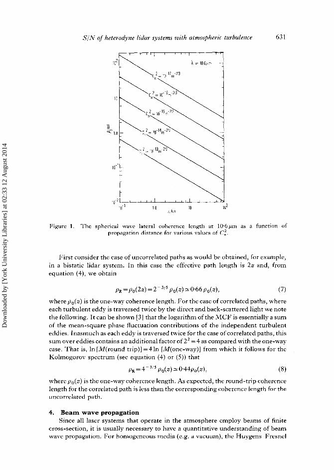
and is plotted in figure 1 as a function of z for )L =10.6 µm and various values of C2, .For propagation near the ground over distances of the order of a few kilometers, weobtain a value of p o of the order I m (at 10 .6 gm) . The corresponding value of p o atother wavelengths is obtained from equation (5) as

,(µm) 6/5Po(A) =Po(10 - 6 Pm)

C 10 ,6 ]

(6)

For example, p o (3 .7µm) -0 . 28 p o(10 .6pm) .The expressions for p o given by equations (4) and (5) are for a one-way path . In

lidar applications we are concerned with a round-trip path, and we present thecorresponding expressions for p o . As will be shown below, the round-trip coherencelength pR appropriate to lidar heterodyne systems results from the case where thepoint source is located at the scattering region of interest and evaluated at the lidarlocation .

Dow

nloa

ded

by [

Yor

k U

nive

rsity

Lib

rari

es]

at 0

2:33

12

Aug

ust 2

014

S/N of heterodyne lidar systems with atmospheric turbulence

631

Figure 1 . The spherical wave lateral coherence length at 10 .6 pm as a function ofpropagation distance for various values of C„ .

First consider the case of uncorrelated paths as would be obtained, for example,in a bistatic lidar system . In this case the effective path length is 2z and, fromequation (4), we obtain

PR = Po(2z) = 2 -35 Po(z) ^-' 0.66 Po(z),

(7)

where po(z) is the one-way coherence length. For the case of correlated paths, whereeach turbulent eddy is traversed twice by the direct and back-scattered light we notethe following . It can be shown [3] that the logarithm of the MCF is essentially a sumof the mean-square phase fluctuation contributions of the independent turbulenteddies . Inasmuch as each eddy is traversed twice for the case of correlated paths, thissum over eddies contains an additional factor of 2 2 =4 as compared with the one-waycase. That is, In [M(round trip)] = 4 In [M(one-way)] from which it follows for theKolmogorov spectrum (see equation (4) or (5)) that

PR=4 315 Po(z)^_- 0 . 44Po(z),

(8)

where po(z) is the one-way coherence length. As expected, the round-trip coherencelength for the correlated path is less than the corresponding coherence length for theuncorrelated path .

4 . Beam wave propagationSince all laser systems that operate in the atmosphere employ beams of finite

cross-section, it is usually necessary to have a quantitative understanding of beamwave propagation. For homogeneous media (e.g . a vacuum), the Huygens-Fresnel

Dow

nloa

ded

by [

Yor

k U

nive

rsity

Lib

rari

es]

at 0

2:33

12

Aug

ust 2

014

632

H. T. Yura

formulation is an excellent approximation for the optical field in space when thepropagation distance is much larger than the physical size of the transmittingaperture (as it is for all cases of practical interest) . The Huygens-Fresnel principlerepresents the optical wavefunction as a coherent sum of elementary spherical wavecontributions over the transmitting aperture, each of which are weighted by the(complex) transmitting aperture wavefunction . In this manner, the resulting opticalwavefunction is related directly to the source variables . The Huygens-Fresnelprinciple is general in that it is valid for an arbitrary source distribution and in boththe near and far fields of the transmitting aperture . The Huygens-Fresnelformulation is particularly suitable for atmospheric propagation because it can beextended directly to an inhomogeneous or turbulent medium [7] .

If the (scalar) optical field at propagation distance z and transverse coordinate p isdenoted by U(p, z), then from [7] we have that

U(p Z) = ( Z~ . )exp[iYs(r p)]

Us(r, P) UA(r) d2 r,

(9)

where the integration extends over the transmitting aperture, s(r, p) is the distancebetween the field coordinate (p, z) and the aperture coordinate (r, 0), UA(r) is the(assumed known) transmitting aperture wavefunction and Us(r, p) contains all theeffects of the turbulent medium on spherical wave propagation . The quantityexp (iks)ls is the spherical wavefunction in the absence of turbulence and Usrepresents the additional spherical wavefunction perturbation produced by theturbulent medium . In practice, the paraxial approximation is used where in theexponential terms of equation (9) we set

s(r,p)=z+I (r-p)2

and set s = z in the denominator . Note that the case of propagation in the absence ofturbulence is obtained by setting Us= 1 in equation (9) .

In many cases we are concerned with the mean irradiance profile I(p, z)=<IU(p, z)I 2 > where, in general, the angular brackets indicate that we must averageover the medium variables and source variables (e .g . a partially coherent source) . Weassume that the source and medium are uncorrelated, from which is follows that theindicated averaging reduces to a product of averages, one for the medium and one forthe source. The final result is that

k 2d2

kI(p, z) = 271Z

PMn(P)Ms(P, z) exp -i ~ P - P ,

where

P= I IUA(r)I 2d 2 r 2 =transmitted power,

(11)

'VIA(P)=PJ(UA(R+1p)Un(R-ip)>souroeexp(-ikp . R/z) d2 R (12)

and

Ms(p) _ < Us (r l , p) Us (r2, P)>medium,

wherep=r1 -r2 .

Dow

nloa

ded

by [

Yor

k U

nive

rsity

Lib

rari

es]

at 0

2:33

12

Aug

ust 2

014

O.A .

S/N of heterodyne lidar systems with atmospheric turbulence

633

An examination of equation (12) reveals that Ms is just the spherical-wave MCFwhere the point source is located at the point of observation (i .e . p) and evaluatedover the transmitting aperture . For propagation in the absence of turbulence, Ms =1and equation (10) reduces to the well-known Huygens-Fresnel principle inhomogeneous media. Note that for a deterministic source (such as a laser), theindicated average over source variables in equation (12) becomes just the product ofthe indicated deterministic wavefunctions .

As indicated in equation (10), the spherical-wave mutual coherence functionplays a central role in propagation through turbulence . Basically, it describes thereduction in lateral coherence between different elements of the transmittingaperture, effectively transforming it into a partially coherent radiator, the degree ofcoherence decreasing with increasing propagation distance through the medium . Ingeneral, the resulting mean irradiance distribution in space is characteristic of acoherent aperture of dimension po(z), where p o is the lateral coherence length of thespherical wave whose origin is at the point of observation . If p o is smaller than thephysical aperture diameter D, the resulting mean radiation pattern is characteristicof that of an aperture of size po rather than D. Thus, for example, in the far field oneobtains an angular spread of the order of Alpo for p o < D, rather than of the order ofA/D .

We now give some illustrative examples of irradiance profiles which will be usedlater in obtaining the S/N in heterodyne lidar systems . Consider the case where thesource wavefunction UA is a (deterministic) gaussian function :

r 2 2 akUA(r) = UO exp

- 2 a2+f

where U O is a constant, k=2ir/2, a is the 1/e intensity radius and f is the (positive)focal length. Negative values of f correspond to a divergent beam whose angle ofdivergence is of the order of a/f. As discussed in §§ 2 and 3 it is customary to introducethe Kolmogorov model for the turbulent refractive index fluctuations, and hence thespherical wave MCF is given by equation (3) as

MS(p) =exp [-(p/po)5/3],

(15)

where p o is given by equation (4) .The resulting mean irradiance profile is obtained by substituting equations (14)

and (15) into equation (10) and performing the indicated integrations . WithMs givenby equation (15), closed-form expressions can be obtained in terms of confluenthypergeometric functions . The resulting expression is awkward in that it is difficultto extract a physical interpretation . In order to obtain an analytic approximation interms of well-known functions, we approximate 3 in the exponent of equation (15) by2. The resulting integrals then become quadratic in the exponent, permitting theintegrations to be performed by completing the square . The result is that

P

p 2

1(p, z)jai (z)

eXP

a2(z)

(16)

where

P=ita 21U0 1 2 =transmitted power

and

3 A

Dow

nloa

ded

by [

Yor

k U

nive

rsity

Lib

rari

es]

at 0

2:33

12

Aug

ust 2

014

634

H. T. Yura

1 .0

z

fdx e-,-IgxI

516

0

M- fdxe

x gx __

0

l+q

Figure 2 . Comparison of the integral that results by retaining 3 in the exponent of equation(15) to the corresponding integral obtained by replacing 3 by 2. The quantity q is adimensionless parameter that is the same for both cases .

z 2

z 2

2z 2a2 (z)=a 2 1

f

)2 +ka

) + C kpo

(17)

The result given in equation (16) is an excellent approximation, as can be seen fromfigure 2, where we have plotted the integral that results by retaining 3 in the exponentin equation (15) and compared it to the corresponding integral with 3 replaced by 2 .

A physical interpretation of the irradiance pattern can now be readily obtainedfrom an examination of equation (16) . The mean irradiance profile is, to an excellentapproximation, gaussian with a 1/e `spot size' given by a i(z) . Furthermore, anexamination of equation (17) reveals that a,(z) consists of three independent terms .The third term on the right-hand side of equation (17) is the effect of the turbulentmedium and, for po << a, it is seen that, for z >> ka, the resulting far-field spot size is ofthe order of ),z/po , in agreement with the qualitative discussion given previously . Wenote that the corresponding irradiance profile in the absence of turbulence isobtained from equation (17) by setting p o=x . That is, the mean irradiance isgaussian with a 1/e spot size a o (z), given by

a02(Z) =a2(1 - z-)z + ( z )2

- (18)f

ka

Another example of the utility of the use of the Huygens-Fresnel principle, andone that is needed in the derivation of the S/N of a heterodyne lidar system, is thecalculation of the mutual coherence function that results from an incoherent sourcedistribution of finite extent in the absence of turbulence . The field from an arbitrarysource in the absence of turbulence is obtained from equation (9) by setting U s =1 as

k

exp [iks(r, p)]2U(p, z) = (2i)

nUA(r)

s(r,p) d r

k eP(ikz) l JUA(r) exp[~z (r _ p)2 d2 r,

(19)

where the paraxial approximation for s(r, p) has been employed . The MCF in thiscase is

Dow

nloa

ded

by [

Yor

k U

nive

rsity

Lib

rari

es]

at 0

2:33

12

Aug

ust 2

014

S/N of heterodyne lidar systems with atmospheric turbulence

635

M= < U(p 1 , z) U*(p 2 , z)>sourcek 2

=(2xz) J d2rid2 r2<UA(rl)UA(r2)>source

xexpzk2z {(r1 - p1)2- (r2 - P2)2 }

For a statistically stationary source we have that

< UA(rl) UA(r2)>source =Bs(rl - r2),

(21)

where Bs, the source correlation function, is a function of r 1 -r2 . For a given sourcecorrelation function one can obtain, from equations (20) and (21), the resultingMCF. Here, however, we consider an incoherent source where

Bs(r 1 - r2 ) = 6(r 1 - r2)Is(r1),

(22)

where b(r) is the Dirac delta function and Is(r) is proportional to the sourcebrightness distribution . On substituting equation (22) into equation (20), we obtain

( k 2

ik

kM = 2~z

exp 2z {pi -p z} x Is(r) exp -izp • r d 2 r,

(23)

where p=p1 -P2 . In order to proceed further, we choose a gaussian function for I s :

Is exp (- r2/rs ),

(20)

(24)

where rs is the 1/e spot radius of the source distribution . On substituting equation(24) into equation (23) and performing the integration, we obtain, after normalizingthe MCF to unity for p=0,

M(p,z)=

<U(plz)U*(p2,z)>

-exp( -p 2/ps),

(25)V [j U(pl, z)I 2]J[l U(p2, z)1 2] -

where

2zPs--'

(26)s

We obtain a gaussian-shaped MCF with a coherence length p s given by equation(26) . We see that the radiation field due to an incoherent source becomes partiallycoherent, with a coherence length that increases with increasing propagationdistance. One can understand the cause for this from the following physicalconsideration . Very close to the source (i .e . z--+0) the field is essentially incoherent,as is exhibited by equation (26) (i .e . ps~0). On the other hand, consider the source tobe at a very large (i .e . infinite) distance. In this case the source can be considered to bea point and the resulting radiation field is completely coherent, again in accord withequation(26) (i .e . p s --•oo). If for a numerical example, we consider the Sun at~ =10 .6 µm we obtain p s ~_- 0.2 mm. Equation (23) is essentially a statement of thewell-known van Cittert-Zernike theorem [8] .

5 . Signal-to-noise ratio in heterodyne lidar systemsConsider the situation illustrated in figure 3 . A laser beam is transmitted towards

a remote scattering region of interest (e.g . pollutants emitted from a smoke stack, or

3A 2

Dow

nloa

ded

by [

Yor

k U

nive

rsity

Lib

rari

es]

at 0

2:33

12

Aug

ust 2

014

636 H. T. Yura

TRANSMITTER

RECEIVER

\

TURBULENCE SCATTERINGREGION

Figure 3 . Schematic illustration of heterodyne lidar remote sensing configuration .

topographical regions such as forest or vegetation) . The back-scattered light iscollected by a receiving aperture and mixed with a suitable local oscillator referencefield, as indicated by the dashed line in figure 3 . As discussed in § 1, the receiver maybe coaxial with the transmitter . Depending on the laser, continuous-wave or pulsedtransmitting systems may be employed . In any case, one averages over times whichhave long compared to atmospheric fluctuation times to obtain a favourable S/N(many pulses for a pulsed system) . Here we assume that the intervening spacebetween the lidar system and the scattering region is characterized by clear-airturbulence only .

In heterodyne detection it can be shown that [1, 9]

S/N _ < jij 2 >,

(27)

where i is the information-carrying part of the current in the photodetector load .Implicit in equation (27) is an average over a time which is long compared to thereciprocal (Doppler) bandwidth of the signal field . The information-carrying part ofthe current is proportional to the product of the signal field and the local oscillatorfield, integrated over the receiving aperture, i .e .

i= constant f U(r)UR(r) d2 r,

(28)

where U(r) is the signal field, UR is the reference local oscillator field, and theintegration is carried out over the receiving aperture .

On substituting equation (28) into equation (27), and performing the averageover the statistics of the medium, yields

S/N = constant< f f U(r l )U*(r2)UR(r 1 )UR(r2)d2 r id2 r 2 >

=constant f f M(r t -r2)UR(r l)UR(r 2)d2 r l d2 r2 ,

(29)

where M(r) is the mutual coherence function of the signal field at the receiveraperture plane . An examination of equation (29) indicates that the MCF plays acentral role in the determination of the S/N . Changing the integration variables tosum and difference coordinates permits the integration over the sum coordinate to beperformed directly, with the result that

S/N=constant f M(p) WR(p) d 2p,

(30)

where

WR(P)= f UR(r+21P)UR(r -zp)d2 r

(31)

is the receiver weighting function . Although it is possible to carry through theanalysis for an arbitrary UR , it is convenient to assume UR to have a gaussian shape .This choice for UR , together with the gaussian-shaped wavefunction of equation (14)

Dow

nloa

ded

by [

Yor

k U

nive

rsity

Lib

rari

es]

at 0

2:33

12

Aug

ust 2

014

S/N of heterodyne lidar systems with atmospheric turbulence

637

for the laser output field, permits us to obtain analytic results in terms of algebraicfunctions . Specifically, we assume that

UR-exp (r 2/2b2 ),

(32)

where b is the 1/e intensity radius of the local oscillator reference field . Substitutingequation (32) into equation (31) and performing the integration yields

WR(p) =7Cb2 exp (-p2/4b2 ) .

(33)

Since we are interested primarily in turbulence effects, we first compute thereduction factor i(,< 1) by which the S/N is reduced in the presence of turbulence ascompared to the corresponding case in the absence of turbulence . Denoting by thesubscripts t and 0 the presence and absence of turbulence, the reduction factor tl1 isdefined as

~_(S/N)~

(34)(S/N)o

Substituting equations (30) and (33) into equation (34) yields

_ fMM(p)eXp( p 2/4b2)d2 p

f

(-

(35)Mo(p) eXp p2/4b2)d2P

where M, and Mo are the MCFs at the receiving aperture that result in the presenceand absence of turbulence, respectively .

Consider first the absence of turbulence . We assume an output laser field as givenby equation (14) . This beam illuminates the scattering region, which is assumed tobe located at a propagation distance z . The light which is (incoherently) back-scattered at every point in the scattering region is, among other things, proportionalto the incident irradiance at that point . Since the scattering particles are at randompositions with respect to each other, the back-scattering source distribution can betaken to be mutually incoherent and to have a brightness distribution proportional tothe incident irradiance distribution . In the absence of turbulence, and for a gaussianlaser source distribution, we have shown that

Io(p, z)=~a2z)exp[ -p2/ao(z)],

where ao(z) is given by equation (18) . That is, as far as the back-scattered light isconcerned, we have essentially a gaussian-shaped incoherent source distribution of1/e spot radius ao(z) . Hence we may apply directly the results given by equations (25)and (26), with rs =ao(z), to obtain the MCF as

and ao is given by equation (18) .In the presence of turbulence, we may obtain M, by the following considerations .

With turbulence present, the mean irradiance pattern is now given by equation (16),where the spot size a,(z), given by equation (17), is greater than the corresponding

whereMo(p) = exp (- p2/Pso), (36)

2zPso = kao(z)

(37)

Dow

nloa

ded

by [

Yor

k U

nive

rsity

Lib

rari

es]

at 0

2:33

12

Aug

ust 2

014

638

11 . T. Yura

spot size a o(z) in the absence of turbulence . The turbulence has spread the beam anda larger spot size results at the scattering region of interest . We note that theappropriate coherence length p o that appears in the expression for a, is for the casewhere the point source is located at the scattering region of interest (see thediscussion following equation (13)) . In addition, as the back-scattered light travelsback towards the receiver, it now propagates through the turbulent atmosphere and anadditional loss of coherence of the wave is incurred . Therefore, the resulting MCF inthe presence of turbulence is given by

Mt(P, z) = M11(P, z)Mt2(P, z),

whereMt1 is the MCF that results from an incoherent source distribution of spot sizea,(z), and Mt2 is the additional MCF that results as the back-scattered lightpropagates through the turbulent atmosphere to the receiver . From our previousdiscussion, we have that

where

Mt1 =exp ( - P 2 /Pst),

2zPst= ka,(z)

(38)

(39)

a t(z) is given by equation (17) and

Mt2 =exp [-(P/Po)513],

(40)

where p o , given by equation (4), is the lateral coherence length of a point sourcelocated in the scattering region . Note that both the p os that appear in equations (39)and (40) have their origins in the scattering region .

On approximating 5 in the exponent of equation (40) by 2, substituting equations(36) to (40) into equation (35) and performing the resulting gaussian integrals, wefind that

a 2 [1- (z/f)] 2 + (z/ka) 2 + (z/kb)2

(41)a 2 [1 - (z/f)] 2 + (z/ka) 2 + (z/kb) 2 + (2z/kp R) 2 '

where P R is the round-trip coherence length of a point source located at the scatteringregion and is given explicitly for both uncorrelated and correlated paths by equations(7) and (8) respectively . Equation (41) is general in that it is valid for receiver andtransmitter aperture radii of different sizes, for both the near and far field of thetransmitting aperture, for laser beams of arbitrary focal length and for an arbitrarypropagation path through the turbulent atmosphere .

For illustrative purposes we consider the special cases of both focused (f = z) andcollimated (f = oo) coaxial systems (a = b) in the presence of uniform turbulenceconditions where the one-way coherence length p o(z) is given by equation (5) . Theresults presented below are expressed in terms of the more commonly used 1/e2intensity radii a2(= .Ja) .

Focused coaxial system (z=f)We obtain

142

1 + (a2/PR) 2

Dow

nloa

ded

by [

Yor

k U

nive

rsity

Lib

rari

es]

at 0

2:33

12

Aug

ust 2

014

S/N of heterodyne lidar systems with atmospheric turbulence

639

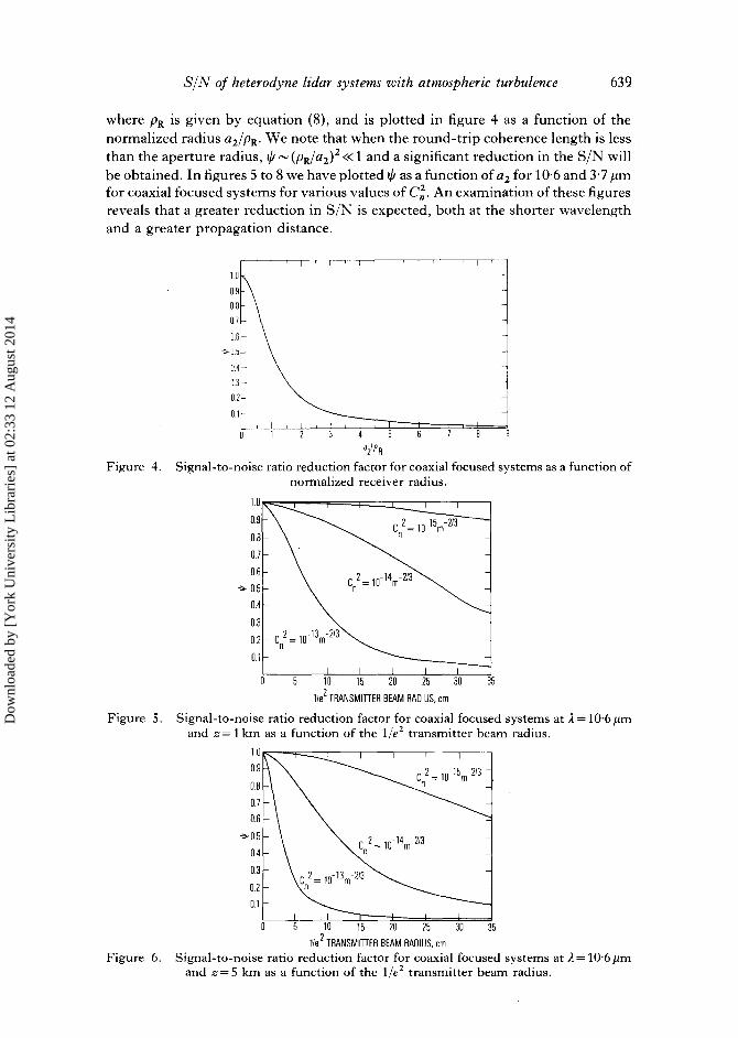
where PR is given by equation (8), and is plotted in figure 4 as a function of thenormalized radius a2/pR . We note that when the round-trip coherence length is lessthan the aperture radius, t0-(pR/a2 ) 2 <<1 and a significant reduction in the S/N willbe obtained . In figures 5 to 8 we have plotted 0 as a function of a2 for 10 . 6 and 3 .7 pmfor coaxial focused systems for various values of C,2, . An examination of these figuresreveals that a greater reduction in S/N is expected, both at the shorter wavelengthand a greater propagation distance .

1

2

3

4

5

a2 1 pRFigure 4 . Signal-to-noise ratio reduction factor for coaxial focused systems as a function of

normalized receiver radius .1 .00 .90 .80 .70 .6

3 0 .5

0 .4

0 .3

0 .2

0.1

5

10

15

20

25

30

lie2TRANSMITTER BEAM RADIUS, cm

Figure 5 . Signal-to-noise ratio reduction factor for coaxial focused systems at A= 10 .6 µmand z=1 km as a function of the 1/e 2 transmitter beam radius .

0 35

0

10

15

20

25

30

35

lie 2 TRANSMITTER BEAM RADIUS, cmFigure 6 . Signal-to-noise ratio reduction factor for coaxial focused systems at A=10 .6 pm

and z=5 km as a function of the 1/e 2 transmitter beam radius .

Dow

nloa

ded

by [

Yor

k U

nive

rsity

Lib

rari

es]

at 0

2:33

12

Aug

ust 2

014

640

1 .0U .90.80.70.60.50.40 .30 .20.1

0

10

15

20

25

30

3511e2 TRANSMITTER BEAM RADIUS, cm

Figure 7 . Signal-to-noise ratio reduction factor for coaxial focused systems at A=3-7µmand z=1 km as a function of the 1/e2 transmitter beam radius .

Collimated coaxial system (f=co)We obtain

_

1+1821 + 262[1 + (a2/pR)2]'

(43)

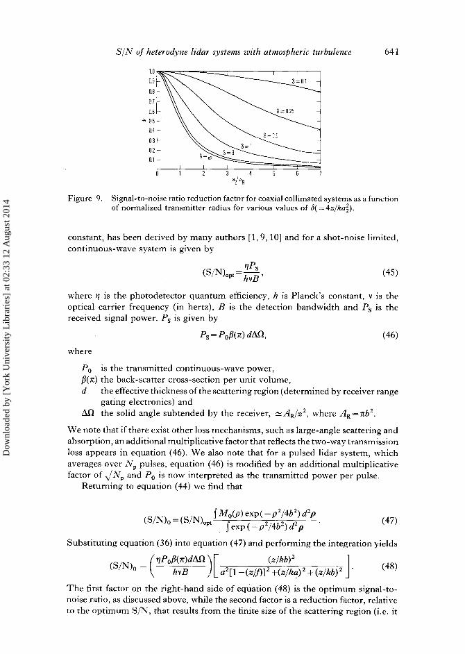
2where d =4z/ka, and is plotted in figure 9 as a function of a2/PR for various values of6. The cases S << 1 and 6 >> 1 correspond to the near and far fields respectively . Anexamination of equation (43) reveals that in the far field the reduction factor for thecollimated case reduces to that of the focused case (this is also clear from figure 7) .

Having derived the turbulence-induced reduction factor t/i, we now return toequation (30) and calculate the signal-to-noise ratio in the absence of turbulence,(S/N)o. From equations (30) and (33), we have

(S/N)o=constant f MO(p)exp(-p2/4b2)d2p,

(44)where Mo is given by equation (36) .

To proceed further, we note that if the signal field were completely coherent withrespect to the local oscillator reference field over the receiving aperture, one wouldobtain the optimum signal-to-noise ratio that could be achieved . The optimumsignal-to-noise ratio, obtained when the signal-field mutual coherence function is

H. T. Yura

5

10

15

25

3D

35lie 2 TRANSMITTER BEAM RADIUS, cm

Figure 8 . Signal-to-noise ratio reduction factor for coaxial focused systemsand z=5 km as a function of the 1/e2 transmitter beam radius .

at ~=3.7pm

Dow

nloa

ded

by [

Yor

k U

nive

rsity

Lib

rari

es]

at 0

2:33

12

Aug

ust 2

014

S/N of heterodyne lidar systems with atmospheric turbulence

641

3

0 I 2 3

4

8 21 PR5 6 7

Figure 9 . Signal-to-noise ratio reduction factor for coaxial collimated systems as a functionof normalized transmitter radius for various values of 6(=4z/kaZ) .

constant, has been derived by many authors [1, 9, 10] and for a shot-noise limited,continuous-wave system is given by

(S/N)°P`= h B ,

( 45)

where t1 is the photodetector quantum efficiency, h is Planck's constant, v is theoptical carrier frequency (in hertz), B is the detection bandwidth and Ps is thereceived signal power . Ps is given by

Ps =Po/1(n) dM,

(46)where

Po is the transmitted continuous-wave power,/3(n) the back-scatter cross-section per unit volume,d

the effective thickness of the scattering region (determined by receiver rangegating electronics) and

M2 the solid angle subtended by the receiver, ^--AR/z 2 , where AR =mtb 2 .

We note that if there exist other loss mechanisms, such as large-angle scattering andabsorption, an additional multiplicative factor that reflects the two-way transmissionloss appears in equation (46) . We also note that for a pulsed lidar system, whichaverages over NP pulses, equation (46) is modified by an additional multiplicativefactor of JNP and Po is now interpreted as the transmitted power per pulse .

Returning to equation (44) we find that

(S/N)o=(S/N)O,, fMo(p)exp(2pz/4b2) dzp .

(47)f exp (-p /4b) d p

Substituting equation (36) into equation (47) and performing the integration yields

S

t1Pol3(7r)d0~(z/kb) z( /N)o =

hvB

a2[1 -(z/J)]2+(z/ka)2+(z/kb)2

(48)

The first factor on the right-hand side of equation (48) is the optimum signal-to-noise ratio, as discussed above, while the second factor is a reduction factor, relativeto the optimum S/N, that results from the finite size of the scattering region (i .e . it

Dow

nloa

ded

by [

Yor

k U

nive

rsity

Lib

rari

es]

at 0

2:33

12

Aug

ust 2

014

642

H. T. Yura

reflects the fact that the signal field, even in a homogeneous medium, is partiallycoherent over the receiving aperture and hence optimum mixing between the signaland local oscillator fields does not occur) .

We now combine equations (34), (41) and (48) to obtain the final general result forthe signal-to-noise ratio of a heterodyne lidar system in the presence of turbulence as

(S/N)t = (S/N)oi

rjPo/3(ir) dAS2,

(z/kb) 2hvB

)[a 2[1-(z/f)]2+(z/ka)2+(z/kb)2+(2z/kpR)2]' (49)

where all the terms appearing in equation (49) have been defined previously .In general, atmospheric turbulence will eventually limit severely the perform-

ance of heterodyne lidar systems. Indeed, an examination of equation (49) revealsthat, for strong turbulence conditions such that pR <<a and b, the (S/N) t -pR, wherewe have used the fact that the solid angle subtended by the receiver optics isproportional to the area of the receiver aperture . This is in contrast to the absence ofturbulence, where (S/N) o increases with increasing area of the receiver apertureoptics, reaches a maximum value when the receiver aperture area is of the order thesquare of the Fresnel length (i .e . -z/k), then decreases with increasing values ofreceiver aperture area . This latter behaviour is expected because in the near field ofthe source the received signal field becomes progressively more incoherent as thereceiver aperture area increases relative to the square of the Fresnel length . In the farfield, the signal-to-noise ratio in the presence of turbulence tends asymptotically to aconstant with increasing receiver aperture area .

These results can be demonstrated clearly by considering the case of a coaxial(a = b) collimated system . On substituting AQ =nb 2/z 2 and f=cc into equation (49)we find that the signal-to-noise ratio can be written as

x 2(S/N),=C 1 +2x4+s2x2 ,

(50)

where

C=io Pof(n)dkhvBza2

I -yj(4z/k)

(51)

J(4z/k)PR

and a 2 is the 1/e 2 transmitter/receiver aperture radius . The quantity x is essentiallythe initial beam radius divided by the Fresnel length . The effects of turbulenceon the signal-to-noise ratio is contained in the parameter e . The absence of turbu-lence corresponds to e=0, while strong turbulence conditions correspond toex=a 2/pR>> 1 . In figure 10 we present a plot of the relative signal-to-noise ratio as afunction of the normalized receiver aperture radius x for various values of theturbulence parameter e .

An examination of equation (50) and figure 10 reveals that (S/N) reaches amaximum value equal to (2,x/2+E2)-1 at x=(2)_

1/4,i .e . a2 =(2v/2 z/k) 1 / 2 . Fore>> 1,

Dow

nloa

ded

by [

Yor

k U

nive

rsity

Lib

rari

es]

at 0

2:33

12

Aug

ust 2

014

S/N of heterodyne lidar systems with atmospheric turbulence

643

Figure 10. Signal-to-noise ratio for coaxial collimated systems as a function of normal-ized beam radius x (=a/J(4z/k)) for various values of the turbulence parametera(= J(4z/k)/pR) . The figures shown above are plots of the quantity within parentheseson the right-hand side of equation (50) for various values of a .

the maximum achievable value of the signal-to-noise ratio is inversely proportional

to a2 (i .e . pR--*0) . Furthermore, for strong turbulence conditions, the signal-to-noiseratio remains essentially constant over a wide range of values of receiver radius a2 , instrong contrast to the absence of turbulence (see figure 10). For a numerical example,

consider the case of propagation at i = 3 .7 µm, a one-way path length z of 5 km,C„ =10 14 m -2/3 and a2 =15 cm. From equations (51) and (8) we obtain x 1 .38 anda 4.9. Hence, from equations (50) we obtain a signal-to-noise ratio relative to that of

the constant C of 0 .035, as compared to the corresponding value in the absence ofturbulence of 0 .23 .

In addition, we present results for the signal-to-noise ratio for a coaxial (a= b)focused system. On substituting ALI= rzb2/z 2 and z =f equation (49), we find that thesignal-to-noise ratio can be written as

x2(S/N),=C

1+E2x2

(52)

where C, x and a are given by equations (51) . In figure 11 we present a plot of therelative signal-to-noise ratio as a function of the normalized receiver aperture radiusx for various values of the turbulence parameter a . In the absence of turbulence(a=0) the signal-to-noise ratio increases as the square of the receiver aperture radius(i .e . receiver aperture area) . For finite a, the signal-to-noise ratio levels off for ax > 1(i .e . pR < a2 ), and tends asymptotically to a constant (proportional to P R) which tendsto zero for strong turbulence conditions. For a numerical example, we use the samevalues of the parameters that were used for the collimated case given above . Weobtain a signal-to-noise ratio relative to the constant C of 0 . 041, as compared to thecorresponding value in the absence of turbulence of 1 .89 .

Dow

nloa

ded

by [

Yor

k U

nive

rsity

Lib

rari

es]

at 0

2:33

12

Aug

ust 2

014

644

S/N of heterodyne lidar systems with atmospheric turbulence

10 1

10-3

10

10

10

010 - 0 10

E=10

E= 3 .0

E=10.0

E= 30

E=100

E= 300

10 0

Figure 11 . Signal-to-noise ratio for coaxial focused systems as a function of normal-ized beam radius x(=a21,1(4z/k)) for various values of the turbulence parametere(=V(4z/k)/pR) . The figures shown above are plots of the quantity within parentheseson the right-hand side of equation (52) for various values of e .

In conclusion, we have derived a general expression for the signal-to-noise ratioof a heterodyne lidar system in the presence of atmospheric turbulence which is validin both the near and far fields of the laser and remote scattering source . Although wehave employed a gaussian-shaped laser source and receiver wavefunctions, whichenabled us to obtain the S/N in terms of algebraic functions, the correspondingqualitative behaviour and numerical results for an arbitrarily shaped laser source andreceiver wavefunction are not expected to differ significantly as all of the essentialphysics of the problem are contained in our analysis .

ReferencesHINCKLEY, E . D., 1976, Laser Monitoring of the Atmosphere (Berlin : Springer Verlag) .LEE, R. W., and HARP, J . C., 1969, Proc . Inst . elect . electron . Engrs, 57, 375 .TATARSKII, V . I ., 1971, The Effects of the Turbulent Atmosphere on Wave Propagation(Springfield, Virginia : National Technical Information Service) .

FANTE, R. L ., 1975, Proc. Inst . elect . electron . Engrs, 63, 1669 .PROKHOROV, A. M ., BUNKIN, F . V., GoCHELASVILY, KL .S ., and SHISHOV, V. 1 ., 1975,Proc. Inst. elect . electron . Engrs, 63, 790 .

YURA, H. T., 1972, Appl. Optics, 11, 1399 .LUTORMIRSKI, R. F ., and YURA, H. T ., 1971, Appl. Optics, 10, 1652 .BORN, M ., and WOLF, E ., 1965, Principles of Optics, third (revised) edition (New York :Pergamon Press), p .510 .SEIGMAN, A . E ., 1966, Proc. Inst. elect . electron . Engrs, 54, 1350 .FRIED, D . L., 1967, Proc. Inst . elect . electron . Engrs, 55, 57 .

Dow

nloa

ded

by [

Yor

k U

nive

rsity

Lib

rari

es]

at 0

2:33

12

Aug

ust 2

014