Sibling Rivalry: Endowment and IntrahouseholdAllocation in Gansu Province, China ∗

Jessica Leight

September 4, 2014

∗This draft: September 2014. Thanks to the Gansu Survey of Children and Families for access to thedata, to Marcel Fafchamps and Albert Park for extensive feedback, and to Esther Duflo, Paul Glewwe,Rohini Pande, Abhijit Banerjee, Erica Field and seminar participants for numerous helpful suggestions.All errors are my own. Running title: Endowment and intrahousehold allocation. Contact: WilliamsCollege Department of Economics, Schapiro Hall, 24 Hopkins Hall Drive, Williamstown, MA 01267.Phone: 413-597-5032. Fax: 413-597-4045. Email: jessica.leight@williams.edu

1

Abstract

This paper evaluates the strategies employed by households in rural China to allo-

cate educational expenditure to children of different initial endowments, examining

whether parents use educational funding to reinforce or compensate for these dif-

ferences. Climatic shocks are employed as an instrument for endowment, measured

as height-for-age, allowing for the identification of the impact of quasi-exogenous

variation in endowment on parental allocations conditional on household fixed ef-

fects. The results suggest that educational expenditure is directed to the relatively

weaker child; in response to the mean difference in endowment between siblings,

parents redirect around 25% of discretionary educational spending to the child with

lower endowment, and this effect is robust to the potentially confounding effects

of gender and birth order. There is some evidence that time allocation may also

be a relevant margin of compensation, but no evidence that medical expenditure

responds to differences in endowment.

2

1 Introduction

For decades, social scientists have analyzed the decisions households make about human

capital accumulation and the implications of these decisions for individual economic out-

comes (Strauss and Thomas, 1995). Given that the majority of educational investments

are made in childhood, it is particularly crucial to understand the choices that parents

make about education on behalf of their children - choices that, in multichild families,

entail not only identifying resources for education in the form of money or parental time,

but allocating those resources among multiple children.

This paper provides evidence about the parental allocation of resources for education

among children of varying endowments in a low-resource setting in rural China, seeking

to identify whether parents employ a compensatory or a reinforcing strategy in response

to variations in health and physical robustness among their children. However, direct

estimation of the relationship between parental behavior and relative health or ability

poses serious challenges. Any measurement of child characteristics will inevitably include

a component of endogenous parental nurturing, and thus a parental preference may man-

ifest itself in both better health for a given child and in overtly preferential treatment

of the same child. This generates spurious evidence of a positive relationship between a

child’s endowment and parental investments.

The principal methodological contribution of this paper is to address the endogeneity

of children’s measured endowment by employing as an instrument a measure of exoge-

nous variation in resource availability correlated with physical health. The instrument

used is grain yield in utero and in infancy for each child, an index of nutritional avail-

ability during a critical period of childhood development that substantially determines

physical endowment. There is a broad consensus in the existing medical literature that

malnutrition in the first years of life, particularly during the prenatal period and between

birth and age three, has a substantial negative impact on physical and cognitive devel-

opment (Pollitt et al., 1999; Grantham-McGregor and Ani, 2001). Shocks to a child’s

3

nutritional intake in this period are correlated with endowment, but exogenous to other

intrahousehold decisions given the use of household fixed effects that absorb shocks to

the household’s overall budget constraint.

The results show a clear pattern of spending allocations favoring the child with lower

endowment, consistent with a parental preference for equality that seeks to compensate for

variation in endowment induced by early childhood environmental shocks. This pattern

of preferential allocations holds across multiple measures of expenditure, and is robust to

the potentially confounding effects of gender and birth parity. There is also some evidence

that time allocation may be a mechanism for parental compensation. However, parents

do not seem to exhibit compensatory behavior in the allocation of medical expenditure.

Previous literature examining intrahousehold allocation of resources to offspring has

largely focused on the question of differential allocation to male versus female children,

with a substantial literature establishing a pattern of preferential allocations to male

children in both South and East Asia (Hazarika, 2000; Behrman and Deolalikar, 1990;

Ono, 2004). Other studies have examined the impact of the sex ratio of siblings on a

child’s education, finding that a child with more sisters has better health and educa-

tion outcomes than one with more brothers (Garg and Morduch, 1998; Morduch, 2000),

though the inverse relationship appears to hold in the United States (Butcher and Case,

1994). A separate literature has focused on the relationship between birth order and the

intrafamily distribution of resources (Parish and Willis, 1993; Tenikue and Verheyden,

2007; Bommiere and Lambert, 2004).

A smaller literature has analyzed whether parents have a general preference for equal-

ity among their children. An early paper by Griliches presented evidence that parents

attempted to limit intrafamily equality and attenuate preexisting differences in endow-

ment, noting that the effect of IQ on schooling is significantly lower within families

(Griliches, 1979). Behrman, Pollak and Taubman (1982) examine familial allocations

using twin data from the U.S. and reject the pure investment model in which parents

care only about the total return to educational expenditure, employing functional form

4

assumptions on the parental welfare function. Using developing country data, Rosen-

zweig and Wolpin (1988) find that parents in Colombia attempt to compensate for the

disadvantages suffered by children with lower weight at birth by a longer interval prior to

the birth of the next child, though there is contravening evidence that healthier children

are more often breastfed. Behrman (1988) finds evidence in India of a pro-male bias as

well as parental inequality aversion, though such aversion declines in the lean season.

Two more recent papers analyzing the response of parental human capital investments

to children’s variation in endowments found that parents exhibit reinforcing behavior.

Rosenzweig and Zhang (2009) find that parents exhibit higher educational expenditure for

children of higher birth weight in China. They do not address the potential endogeneity

of birth weight for siblings born as singletons - if, for example, children born at a certain

parity or a certain stage of parental development are more wanted, the mothers could

receive better prenatal nutrition, leading to higher birth weight for the child as well as

enhanced subsequent endowments – but find parallel results for twin pairs for which

endogenous determination of birth weight can be ruled out. Conti et al. (2010) also

employ data from China to estimate a structural model of parental resource allocation

given multidimensional child endowments and find evidence of compensating investment

in health but reinforcing investment in education. They exploit early health shocks,

defined as a reported episode of serious disease, assumed to occur randomly within twin

pairs.

In employing climatic shocks at birth as a source of variation in children’s health

endowment, this paper joins a robust literature that has examined the impact of early

childhood shocks (climatic, economic or political) on longer-term outcomes. Almond et al.

(2006) and Meng and Qian (2009) have analyzed the long-term impact of famine caused

by the Great Leap Forward in China. Almond (2006) and Almond and Chay (2006)

exploit shocks to public health and social policy in the U.S. over time, while Banerjee

et al. (2010) evaluate the impact of income shocks in nineteenth century France caused

by a vineyard-destroying insect. Most similar in spirit to this paper may be the work

5

of Maccini and Yang (2009) showing a relationship between early childhood shocks and

long-run economic impacts in Indonesia. However, this paper is one of the the first in

this literature to show evidence of a relationship between in-utero shocks and physical

robustness as measured by height-for-age.

This paper makes several contributions to the existing literature on parental intra-

household allocation. It is the first study to estimate the response of parental allocations

to quasi-exogenous variation in endowment without relying on the use of twin pairs. In

addition, it builds on the existing literature about early childhood shocks, exploiting

these shocks to address the potential endogeneity of a child’s endowment. Finally, it

provides robust evidence of an effect of climatic shocks even in utero on medium-term

health outcomes as measured by height-for-age.

The paper proceeds as follows. Section 2 presents the data. Sections 3 and 4 present

the main empirical results and robustness checks. The final section concludes.

2 Data

The data set employed in this analysis is the Gansu Survey of Children and Families

(GSCF), a panel study of rural children’s welfare outcomes conducted in Gansu province,

China. The first wave, conducted in 2000, surveyed a representative sample of 2000

children in 20 rural counties aged 9-12 as well as their mothers, household heads, teachers,

principals, and village leaders. The second wave, implemented in 2004, supplemented the

first wave with a sample of the younger siblings and fathers of the target children.

The survey employed a four-stage stratified random sample. First, counties were

selected from the full sampling frame of counties, excluding autonomous minority regions.

Townships within each county (and subsequently, villages within each township) were

ranked according to per-capita income, and a sampling distance calculated taking into

account the relative population of each unit. Two to three townships within each county

and two villages within each township were sampled, yielding 100 villages. 20 children

6

were then sampled in each village, randomly selecting from the cohort of children aged

9-12 during the survey’s first wave.

Gansu, located in northwest China, is one of the poorest and most rural provinces in

China. Per capita income in this sample is around $200 a year, and the mean level of

education observed among parents is only seven years for men and four years for women.

This analysis will focus on a subsample of the families in the survey: those with two

children in the household where both children are observed in the second wave survey.

Here, the child aged 9-12 identified in the first round of the survey is referred to as

the index child; in families where the index child had a younger sibling of school age,

that child was surveyed in the second round. If these two children are the only children

in the household, this constitutes a complete survey of parental allocations and child

endowment, and these households are the primary focus of the analysis. Such complete

data is available on 413 families, and they constitute the relevant subsample. The key

results will also be presented for a slightly larger sample including households where these

two children (the index child and the younger sibling) are the youngest two children of a

larger family.1

Clearly, restricting to a subsample raises some question about external validity. How-

ever, it is important to note that the question of intrahousehold allocation among children

in fact is irrelevant for the majority of the excluded sample, who are single-child house-

holds. These households do not form part of the theoretical sample of interest: households

with a number of children greater than one. The primary results will also be shown to

be robust to including households who have a number of children greater than two.

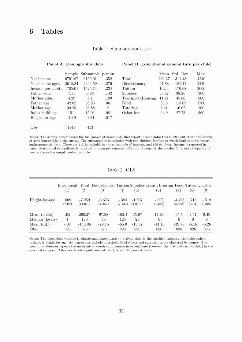
Panel A of Table 1 reports summary statistics for the subsample of two-children

families and the overall sample for key demographic indicators of interest, as well as a t-

test for equality between the two means; no statistically significant difference is apparent

1The average number of children in households in this sample is 2.2. While the One-Child Policy wasin effect during the period in which these children were born, many rural households could nonethelesshave two children legally under various exemptions to the policy (Gu et al., 2007). Other householdsmay simply have defied the rules. It is not possible using this dataset to accurately identify for eachhousehold whether it was in technical compliance with the policy.

7

in income, parental education or the age of the index child. The only significant difference

between the two samples is in parental age. Parents in the subsample are younger,

reflecting the exclusion of households with larger numbers of children and households

who have an older sibling in addition to the index child; these families will generally be

headed by older parents. Height-for-age is also slightly lower in the subsample relative

to the full sample.

The dependent variable of interest is educational expenditure per child per semester,

reported by the head of household in six categories: tuition, educational supplies, food

consumed in school, transportation and housing, tutoring and other fees.2 Each household

reports separately expenditure for each child in each of these categories. In the Chinese

educational context, supplies, tutoring, and other fees correspond to expenditure under-

taken by the household to improve a child’s academic performance, independent of the

school attended. Expenses for transportation, housing and food, on the other hand, may

also vary in accordance with the choice of school and the choice of whether to have a child

board at school or not. Discretionary expenditure is defined as the sum of all expenditure

excluding tuition. Summary statistics for average expenditure per child for the subsample

of families analyzed can be found in Panel B of Table 1. Total educational expenditure

averages slightly less than 300 yuan per child per semester, or a total of 1040 yuan for two

children over a year. This indicates that an average of 16% of mean household income is

allocated to educational expenditure.

The measurement of the child’s endowment is height-for-age, normalized to a Z-score

using the World Health Organization growth charts for children of ages 2-18. Height-for-

age is widely used in the literature as a measure of endowment and a summary indicator of

physical robustness, and it is correlated with a range of physical and cognitive indicators

(World Health Organization, 1995; Grantham-McGregor et al., 2007). It has also been

employed as a measurement of nutritional status and malnutrition for adolescents up to

age 18 (Prista et al., 2003; Sawaya et al., 1995; Leenstra et al., 2005). At the same time,

2In China, textbook fees are mandatory and levied as part of the overall tuition, and here they arelikewise reported in the tuition category. Educational supplies is supplies other than textbooks.

8

evidence suggests it largely reflects the history of nutrition or health prior to age three, as

after this age catch-up for a child stunted in infancy is limited (Martorell, 1999; Alderman,

Hoddinott and Kinsey, 2006). Accordingly, a robust relationship between height-for-age

and early childhood shocks is expected. Summary statistics on height-for-age for the

index child in the sample and the subsample are also shown in Table 1. The average

height-for-age is -1.1, suggesting, perhaps unsurprisingly, that this is a predominantly

stunted population.

The primary data is supplemented by climatic data for Gansu. Grain yield data pre-

1996 is from data tabulated by the Ministry of Agriculture; post-1996, the data is drawn

from annual editions of the Rural Chinese Statistical Yearbook. Grain yield is measured

annually at the county level in tons per hectare.

3 Empirical evidence

3.1 Ordinary least squares

The primary relationship of interest in this analysis is equation (1), where the dependent

variable is the reported expenditure on the education of child i in household h, school

s, county c and born in year t, denoted Eihsct. The independent variable is endowment

as measured by height-for-age, denoted Hihsct. A household fixed effect, denoted ηh,

absorbs any household-level heterogeneity in the propensity for educational spending,

and calendar birth month Monihsct and gender Gihsct are included as controls. The

equation of interest is thus the following:

Eihsct = β1Hihsct + β2Monihsct + β3Gihsct + ηh + εihsct (1)

Because the subsample is composed of two-child families, a household fixed effects

specification is equivalent to estimation of the equation in first differences across the two

children. Any variable that is unchanging within the household (for example, maternal

9

health, the year of birth for either child, and the age gap between the children) is thus

collinear with the household fixed effect ηh. The child-specific error term is denoted εihsct,

and standard errors are clustered at the county level.

The equation is estimated for each of the six categories of educational expenditure,

as well as for a dummy variable for enrollment, total expenditure and total discretionary

expenditure (excluding tuition). The results, shown in Table 2, are generally insignificant.

However, there is the potential for bias in these results if endowment measured at the age

of primary school already embodies a significant component of prior parental investment.

The child who has already been the target of greater parental investment will appear to

have a greater endowment, and, if there is some serial correlation in parental behavior, is

likely to continue to receive more substantial investments. This will generate an upward

bias in the estimated coefficients that may be problematic. Eliminating this bias is the

goal of the identification strategy.

3.2 First stage

The key to identification in this case is the use of a climatic, and thus nutritional, shock

that is correlated with the relative endowment of the two children: grain yield in utero

and in the early years in life. Accordingly, the postulated first stage in its simplest form

is the following, where Sihsct denotes the climatic shock for child i, and month of birth

and gender are again included as controls.

Hihsct = β1Sihsct + β2Monihsct + β3Gihsct + εihsct (2)

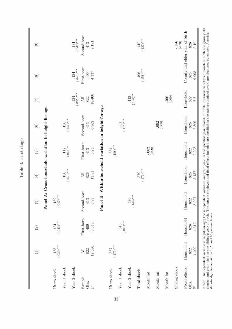
There are 413 pairs of siblings for which anthropometric data is reported, or 826 children.3

Panel A of Table 3 shows the first stage in cross-section, estimating equation (2) with

grain yield in utero and in years one and two of life, respectively, as the independent

3An additional four grain yield observations in a single county-year cell are missing; while no sampledchildren are born in that year, this yields missing observations for the regressions employing data inutero and in the second year of life.

10

variables of interest. All specifications include standard errors clustered at the county

level. Given that grain yield statistics are only reported annually, grain yield in the first

year of life for a given child is calculated as a weighted average of grain yield in the

calendar year of birth and the following year, with the weights depending on the month

of birth; analogous strategies are used to calculate grain yield in the second year of life

and in utero.4

The results show coefficients on grain yield that are positive and significant. Moreover,

there is no significant difference in the impact of the climatic shock experienced over the

three years examined; the pattern detected is entirely consistent. The magnitude suggests

a 25% increase in grain yield relative to the mean in a single year in this critical period

of gestation and infancy leads to an increase in height-for-age of around 6%.

Panel B of the same table shifts the focus to a within-household specification, pre-

senting the results from the first stage estimated with household fixed effects. The spec-

ification is thus analogous to the ordinary least squares specification already estimated.

Hihsct = β1Sihsct + β2Monihsct + β3Gihsct + ηh + εihsct (3)

The results show a positive correlation between the within-household difference in grain

yield in the county and year of birth and the observed difference in height-for-age that is

significant for shocks in utero and in the first and second year of life. In order to maximize

predictive power, I then define the total grain yield shock as the mean of grain yield in

years zero (in utero), one and two, and employ this variable in an analogous regression.

This is the primary first stage of interest, and it can be seen in Column (4) of Panel B.

One potential source of noise in these specifications is the timing of the relevant

harvest vis-a-vis the birth. The definition of the grain yield variable assumes that the

most important shock is the quality of the harvest, as proxied by grain yield, following

4Defining G1 as grain yield in the calendar year of birth and G2 as grain yield in the next calendar year,the climatic shock in the year of birth is defined as G1 for children born in January, 11/12G1 + 1/12G2

for children born in February, and so on. The results of interest are robust to alternate constructions ofthe grain yield variable.

11

conception and birth; thus the measurement of grain yield proceeds forward from the date

of conception or the date of birth and calculates average grain yield for the next nine

or twelve months. However, given that grain crops are primarily harvested in the third

quarter, it is possible that for children conceived later in the calendar year, the most

important harvest actually precedes their conception, generating the grain stock that

subsequently feeds the pregnant mother. (Analogously, one could argue that the most

important harvest for the first year of life could precede birth for children born late in the

year, generating the grain stock that feeds the infant.) In order to test this hypothesis, I

estimate equation (2) adding interaction terms between each of the grain yield variables

and month of birth. The results in Columns (5) through (7) show interaction terms

that are uniformly insignificant, suggesting that heterogeneous effects with respect to the

month of birth are not evident.

The absence of variation with respect to birth month in the relationship between

grain yield and height also suggests that shocks to maternal labor supply are not a

plausible mediating channel for the relationship between climatic channels and health

outcomes. Trias (2013) presents evidence that in Ecuador, positive weather shocks during

the growing season have a negative impact on infant health when they coincide with the

first trimester of pregnancy or the first months after birth, because positive shocks induce

women to provide more agricultural labor and invest less time in activities that enhance

their and their infants’ health. This channel would suggest that children conceived or

born shortly before the growing season should exhibit a different relationship between

climatic shocks and health (either attenuated or of opposite sign) compared to children

born in other seasons, but there is no evidence of this pattern here.

As a robustness check, I also examine whether there is evidence of cross-dependence of

shocks: controlling for his or her own shocks in infancy, the exclusion restriction requires

that there is no dependence of one sibling’s height-for-age on shocks experienced during

the infancy of the other sibling. For example, one major threat to the identification

strategy would be reallocation of resources by households in response to an adverse event,

12

if following the birth of the second child, households preferentially direct resources to

either the first or the second child when a negative shock occurs. This would be evident

in a significant relationship between the older child’s height and the shock to the younger

child.

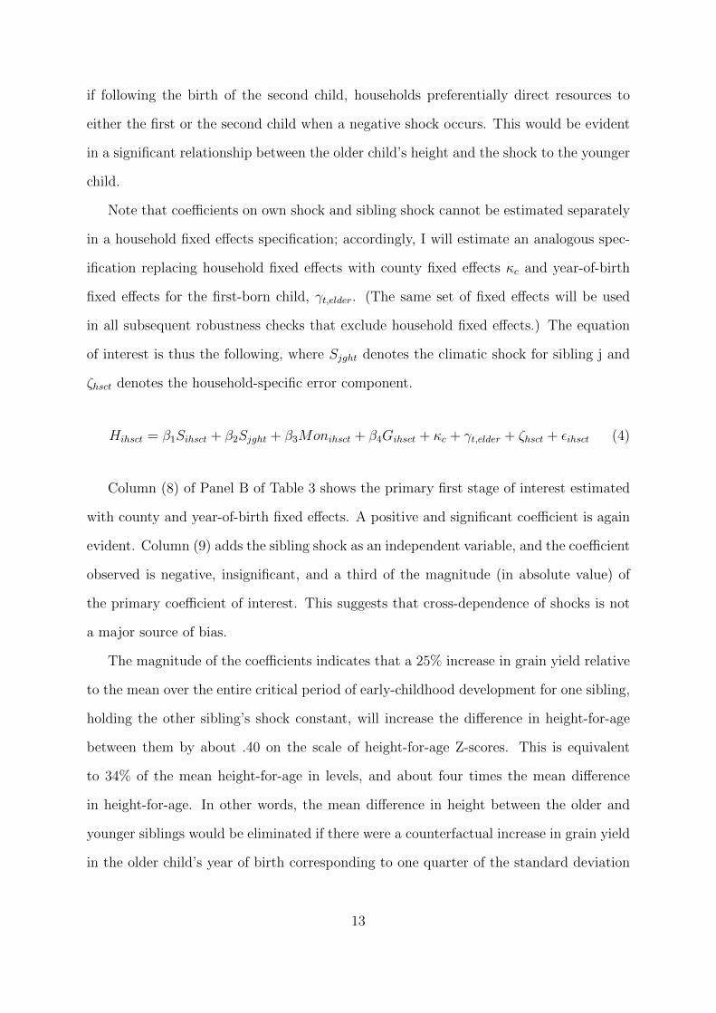
Note that coefficients on own shock and sibling shock cannot be estimated separately

in a household fixed effects specification; accordingly, I will estimate an analogous spec-

ification replacing household fixed effects with county fixed effects κc and year-of-birth

fixed effects for the first-born child, γt,elder. (The same set of fixed effects will be used

in all subsequent robustness checks that exclude household fixed effects.) The equation

of interest is thus the following, where Sjght denotes the climatic shock for sibling j and

ζhsct denotes the household-specific error component.

Hihsct = β1Sihsct + β2Sjght + β3Monihsct + β4Gihsct + κc + γt,elder + ζhsct + εihsct (4)

Column (8) of Panel B of Table 3 shows the primary first stage of interest estimated

with county and year-of-birth fixed effects. A positive and significant coefficient is again

evident. Column (9) adds the sibling shock as an independent variable, and the coefficient

observed is negative, insignificant, and a third of the magnitude (in absolute value) of

the primary coefficient of interest. This suggests that cross-dependence of shocks is not

a major source of bias.

The magnitude of the coefficients indicates that a 25% increase in grain yield relative

to the mean over the entire critical period of early-childhood development for one sibling,

holding the other sibling’s shock constant, will increase the difference in height-for-age

between them by about .40 on the scale of height-for-age Z-scores. This is equivalent

to 34% of the mean height-for-age in levels, and about four times the mean difference

in height-for-age. In other words, the mean difference in height between the older and

younger siblings would be eliminated if there were a counterfactual increase in grain yield

in the older child’s year of birth corresponding to one quarter of the standard deviation

13

of grain yield across counties and years.

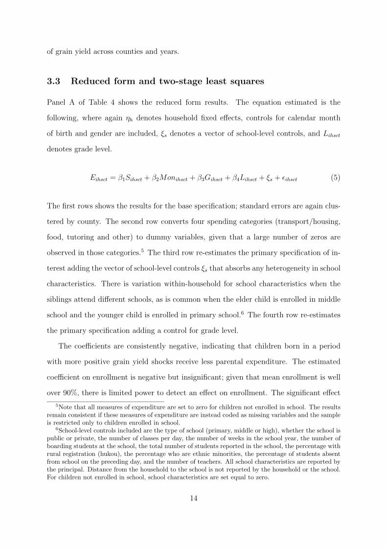
3.3 Reduced form and two-stage least squares

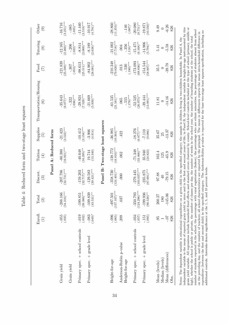
Panel A of Table 4 shows the reduced form results. The equation estimated is the

following, where again ηh denotes household fixed effects, controls for calendar month

of birth and gender are included, ξs denotes a vector of school-level controls, and Lihsct

denotes grade level.

Eihsct = β1Sihsct + β2Monihsct + β3Gihsct + β4Lihsct + ξs + εihsct (5)

The first rows shows the results for the base specification; standard errors are again clus-

tered by county. The second row converts four spending categories (transport/housing,

food, tutoring and other) to dummy variables, given that a large number of zeros are

observed in those categories.5 The third row re-estimates the primary specification of in-

terest adding the vector of school-level controls ξs that absorbs any heterogeneity in school

characteristics. There is variation within-household for school characteristics when the

siblings attend different schools, as is common when the elder child is enrolled in middle

school and the younger child is enrolled in primary school.6 The fourth row re-estimates

the primary specification adding a control for grade level.

The coefficients are consistently negative, indicating that children born in a period

with more positive grain yield shocks receive less parental expenditure. The estimated

coefficient on enrollment is negative but insignificant; given that mean enrollment is well

over 90%, there is limited power to detect an effect on enrollment. The significant effect

5Note that all measures of expenditure are set to zero for children not enrolled in school. The resultsremain consistent if these measures of expenditure are instead coded as missing variables and the sampleis restricted only to children enrolled in school.

6School-level controls included are the type of school (primary, middle or high), whether the school ispublic or private, the number of classes per day, the number of weeks in the school year, the number ofboarding students at the school, the total number of students reported in the school, the percentage withrural registration (hukou), the percentage who are ethnic minorities, the percentage of students absentfrom school on the preceding day, and the number of teachers. All school characteristics are reported bythe principal. Distance from the household to the school is not reported by the household or the school.For children not enrolled in school, school characteristics are set equal to zero.

14

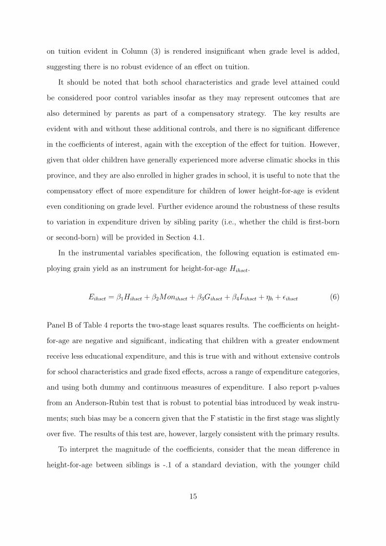
on tuition evident in Column (3) is rendered insignificant when grade level is added,

suggesting there is no robust evidence of an effect on tuition.

It should be noted that both school characteristics and grade level attained could

be considered poor control variables insofar as they may represent outcomes that are

also determined by parents as part of a compensatory strategy. The key results are

evident with and without these additional controls, and there is no significant difference

in the coefficients of interest, again with the exception of the effect for tuition. However,

given that older children have generally experienced more adverse climatic shocks in this

province, and they are also enrolled in higher grades in school, it is useful to note that the

compensatory effect of more expenditure for children of lower height-for-age is evident

even conditioning on grade level. Further evidence around the robustness of these results

to variation in expenditure driven by sibling parity (i.e., whether the child is first-born

or second-born) will be provided in Section 4.1.

In the instrumental variables specification, the following equation is estimated em-

ploying grain yield as an instrument for height-for-age Hihsct.

Eihsct = β1Hihsct + β2Monihsct + β3Gihsct + β4Lihsct + ηh + εihsct (6)

Panel B of Table 4 reports the two-stage least squares results. The coefficients on height-

for-age are negative and significant, indicating that children with a greater endowment

receive less educational expenditure, and this is true with and without extensive controls

for school characteristics and grade fixed effects, across a range of expenditure categories,

and using both dummy and continuous measures of expenditure. I also report p-values

from an Anderson-Rubin test that is robust to potential bias introduced by weak instru-

ments; such bias may be a concern given that the F statistic in the first stage was slightly

over five. The results of this test are, however, largely consistent with the primary results.

To interpret the magnitude of the coefficients, consider that the mean difference in

height-for-age between siblings is -.1 of a standard deviation, with the younger child

15

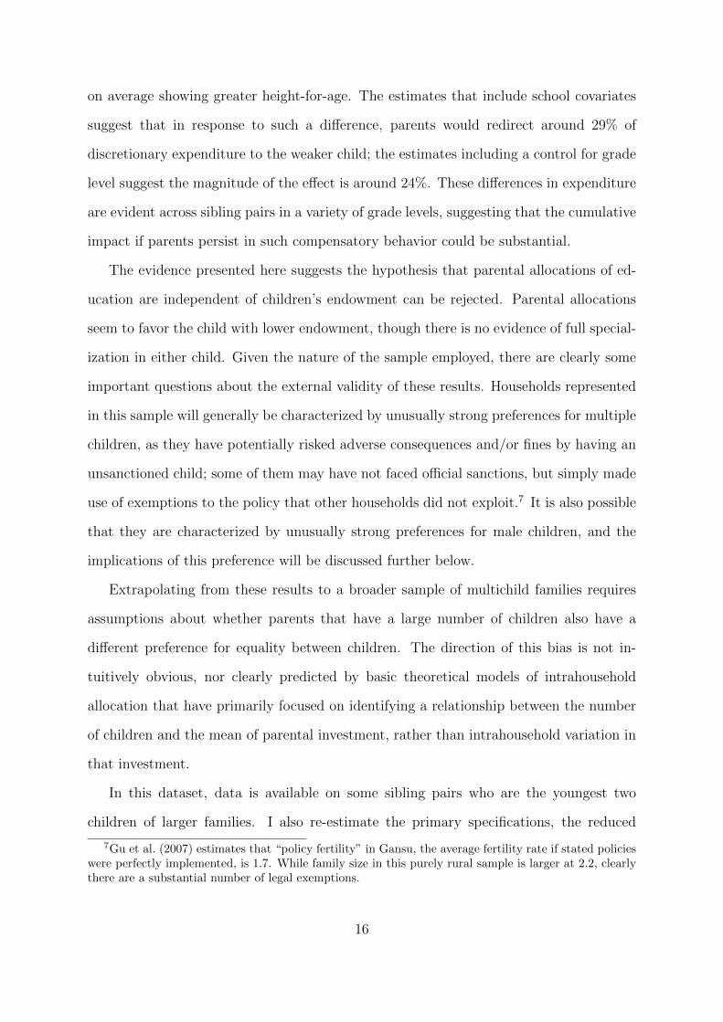
on average showing greater height-for-age. The estimates that include school covariates

suggest that in response to such a difference, parents would redirect around 29% of

discretionary expenditure to the weaker child; the estimates including a control for grade

level suggest the magnitude of the effect is around 24%. These differences in expenditure

are evident across sibling pairs in a variety of grade levels, suggesting that the cumulative

impact if parents persist in such compensatory behavior could be substantial.

The evidence presented here suggests the hypothesis that parental allocations of ed-

ucation are independent of children’s endowment can be rejected. Parental allocations

seem to favor the child with lower endowment, though there is no evidence of full special-

ization in either child. Given the nature of the sample employed, there are clearly some

important questions about the external validity of these results. Households represented

in this sample will generally be characterized by unusually strong preferences for multiple

children, as they have potentially risked adverse consequences and/or fines by having an

unsanctioned child; some of them may have not faced official sanctions, but simply made

use of exemptions to the policy that other households did not exploit.7 It is also possible

that they are characterized by unusually strong preferences for male children, and the

implications of this preference will be discussed further below.

Extrapolating from these results to a broader sample of multichild families requires

assumptions about whether parents that have a large number of children also have a

different preference for equality between children. The direction of this bias is not in-

tuitively obvious, nor clearly predicted by basic theoretical models of intrahousehold

allocation that have primarily focused on identifying a relationship between the number

of children and the mean of parental investment, rather than intrahousehold variation in

that investment.

In this dataset, data is available on some sibling pairs who are the youngest two

children of larger families. I also re-estimate the primary specifications, the reduced

7Gu et al. (2007) estimates that “policy fertility” in Gansu, the average fertility rate if stated policieswere perfectly implemented, is 1.7. While family size in this purely rural sample is larger at 2.2, clearlythere are a substantial number of legal exemptions.

16

form in equation (5) and the two-stage least squares in equation (6), using the larger

sample. The results are shown in Table 5.8 The estimated coefficients are again negative

and significant, and in fact slightly larger in magnitude (though the difference is not

statistically significant). This is suggestive evidence that the observed patterns may

not be limited to two-child families. The opposite exercise might also be of interest:

examining intrahousehold allocation patterns in households with a number of children,

and thus a presumed preference for household size, that is below the mean. Clearly, this

empirical test cannot be implemented using Chinese data given low overall fertility rates.

However, given low or rapidly declining fertility rates characterize much of Europe as

well as the richer Asian economies, patterns of intrahousehold allocation in low-fertility

environments where one-child families are increasingly the norm may still be of interest

from a policy perspective.

3.4 Other outcomes

In this dataset, disaggregated investments by child is reported for only one other category

of spending, investments in medical care. Data is available from two sources: the mother

reports the number of visits to a doctor or to a clinic or hospital for each child, as well as

the number of medical episodes and days of school missed due to sickness for each child,

and separately the head of household (normally the father) separately reports medical

expenses for each child and the number of days ill over the last month.

Investments in health care may be quite different from investments in education: these

investments are rarer (only around half of the sampled children are reported to have uti-

lized any medical care in the previous year), and may respond primarily to short-term

health challenges or emergencies. To test whether medical investments are also responsive

to measures of long-term endowment, I regress the available measures of medical invest-

ment (the number of visits to a doctor and clinic, and actual monetary expenditure)

Emihsct on height-for-age in a specification parallel to the primary specification, estimated

8These estimates do not include the additional controls for school characteristics or grade level.

17

with and without a control for medical necessity as reported by that parent, Mihsct. (For

maternal reports, this is the number of medical episodes or the days of school missed due

to sickness; for paternal reports, this is the number of days ill over the past month.)

Emihsct = β1Hihsct + β2Monihsct + β3Gihsct + β4Mihsct + ηh + εihsct (7)

This specification is estimated using two-stage least squares, instrumenting for height-

for-age with the grain yield shock of interest.

The results are shown in Panel A of Table 6. The coefficients on height-for-age are

small in magnitude and insignificant, while measures of medical expenditure are highly

predictive as expected. This suggests that medical expenditure is not an important

margin for compensation for early childhood shocks.

In addition, the time invested by each household member, including children, in var-

ious activities including leisure, household labor, and homework is reported. Allowing

children to abstain from household chores or spend more time on academic pursuits may

also be plausibly considered a form of parental investment that could be responsive to

children’s endowments. Accordingly, I re-estimate equation (6) with dummy variables

equal to one if a child is reported to invest time in the specified activity as the dependent

variable. Dummy variables are employed given that, with the exception of television, no

more than 50%-60% of children are reported to spend time on each activity enumerated.

Note that there is no adding-up constraint imposed in the data collection procedure; some

parents report that their children spend very few hours on these activities combined, while

the mean total time reported is 22 hours.

The results are shown in Panel B of Table 6. It is evident that children of greater

height-for-age allocate significantly more time to household labor, including chopping

water, fetching wood, and elder care (though the latter coefficient is narrowly insignifi-

cant). They are also significantly less likely to spend time on their own homework. Both

phenomena are consistent with children of lower height-for-age as a result of early child-

18

hood shocks benefiting from a lighter allocation of household labor, and investing more

time in academic work, as a form of parental compensation. The magnitude suggests

that the probability of engaging in chores increases by around 10% in response to the

average difference in height-for-age between children; the probability of investing time in

homework decreases by slightly less than 30%.

Taken together, these results constitute suggestive evidence that time allocation may

be another strategy of parental compensation for children of relatively weaker endowment.

There is, however, no evidence of an effect on investments in health care.

4 Robustness checks

4.1 Sibling parity effects

There is a trend in climatic shocks in Gansu in the period of interest – more specifically,

the mean of the grain yield difference between the first-born and second-born children is

positive. This suggests that sibling parity (i.e., birth order) could be a source of bias in

this specification, if the evident preference for the relatively weaker child in fact reflects

a preference for the first-born child. Accordingly, I re-estimate the primary specification

adding both a linear and quadratic control for sibling parity, Pihsct and P 2ihsct.

Eihsct = β1Hihsct + β2Monihsct + β3Gihsct + β4Pihsct + β5P2ihsct + ηh + εihsct (8)

The results of estimating equation (8) are shown in Panel A of Table 7; standard errors

are again clustered by county. The results show the same negative relationship between

height-for-age and educational expenditure evident in the primary results, and coeffi-

cients on sibling parity that are small in magnitude and generally insignificant. There is

some evidence that first-born children are more likely to be enrolled in school - perhaps

unsurprising, given their older age - and they seem to spend more on school supplies.

19

However, these effects are small in magnitude relative to the estimated coefficients on

height-for-age (with the exception of the coefficient on tuition, where the magnitudes are

comparable).

This suggests that a preference for the first-born child is unlikely to be the primary

omitted variable driving the main results. Comparing the magnitude of the coefficient

on height-for-age to the coefficient estimated in the primary specification, the estimated

coefficients seem to be slightly biased away toward zero, though the difference is not

statistically significant.

4.2 Gender and intrahousehold allocation

A second potential confounding factor is gender. Given the evidence from other sources of

gender bias in household decision-making in China, the effect of gender on parental alloca-

tions may outweigh any observed effect for endowment. While the primary specifications

included gender as a control variable, this may not be regarded as fully satisfactory given

the abundant anthropological and demographic evidence on abortion, abandonment, or

underreporting of female children in China (Coale and Banister, 1994; Qian, 1997); it is

implausible to assume that the gender of both children can be assumed to be random.9

In Gansu, the sex ratio in 2000 was 111.2, close to the national average of 113.6, and

indicative of substantial household determination of child gender (Banister, 2004). Ac-

cordingly, households with different gender balances among their children are likely to

differ materially along other observable and unobservable dimensions.

However, the gender of the first child may be a plausibly exogenous observation, as

anthropological evidence indicates that selection for gender occurs principally in births

subsequent to a first-born daughter, and selective abortion prior to the birth of a first

child is unusual (Gu et al., 2007; Banister, 2004). The evidence in this sample is consistent

with this hypothesis. The sex ratio for the first child is not significantly different from .5,

while for the second-born child, the sex ratio is highly imbalanced: 67% of second-born

9The primary results are also robust to the exclusion of the gender variable.

20

children are male. However, the sex ratio for the second child in households with a first-

born male is likewise not significantly different from .5. Households choosing to bear a

second child following the birth of a son do not engage in costly sex-selection methods in

order to bear a second son.

Accordingly, in households with a first-born son, the gender of both children can

plausibly be considered to be quasi-random. In order to test the robustness of the pri-

mary results to bias introduced by unobservable gender preferences among parents, I

re-estimate the primary specification equation (6) restricting the sample to households

with a first-born son. The estimation results are shown in Table 7, and the pattern of

negative and significant coefficients is consistent with the primary results. While the

coefficients observed are generally somewhat smaller in magnitude, the difference is not

statistically significant.

4.3 Selection bias

Selection into the sample of two-child families observed in this analysis would also con-

stitute a violation of the exclusion restriction. If families with certain characteristics

are more or less likely to suffer an adverse mortality event as the result of the same

climatic shock, then the pattern of shocks may affect the ultimate pattern of allocations

by determining the surviving number of children, and hence inclusion or exclusion in the

sample.

Due to the absence of complete data on retrospective familial mortality, it is not

possible to directly examine child mortality as a function of varying climatic shocks. An

alternative strategy to test for selection effects exploits the presence of extremely severe

climatic shocks that are most likely to be associated with increased mortality. If there is

selective survival among children born in those years, this would be expected to produce

an attenuation toward zero in an otherwise positive relationship between grain yield

shocks and child mortality. This reflects the fact that surviving children, while weakened

by adverse conditions in infancy, are nonetheless likely to be genetically more robust and

21

thus have a propensity toward greater health, weakening the correlation between grain

yield and height-for-age.

On the other hand, if selection via differential mortality is not an important phe-

nomenon, there should not be an attenuation of the relationship between shocks and

health outcomes as the severity of the shock increases - assuming that the relationship

between grain yield and height-for-age is otherwise linear. This is clearly a strong as-

sumption, and accordingly the results should be interpreted with caution.

To test this hypothesis, dummy variables are defined to capture severe climatic shocks

of varying intensity. A severe shock is identified when total grain yield in the critical

period of interest (in utero and in the first and second years of life) falls below the 20th,

30th, 40th, 50th and 60th percentiles, respectively. The first stage equation conditional

on household fixed effects is then re-estimated adding these dummy variables and an

interaction between the dummy variable and the linear grain yield term. For example,

the following equation shows the specification employing a dummy variable for grain yield

below the 20th percentile.

Hihsct = β1Sihsct + β2D20ihsct × Sihsct + β3D

20ihsct + ηh + εihsct (9)

The objective is to test whether the slope of the positive relationship between grain

yield and height-for-age is attenuated toward zero in the lower part of the climatic shock

distribution, a phenomenon that would be evident in a negative coefficient on β2.

The results are shown in Panel A of Table 8. The coefficients β2 are in fact positive

and generally significant, suggesting that selective mortality is not a particularly relevant

phenomenon in this sample. In fact, the positive relationship between grain yield shocks

and height-for-age is larger in magnitude for children in the lower part of the height-for-age

distribution. While these results may partially reflect non-linearities in the relationship

between grain yield and height-for-age independent of selective mortality, the results here

would only be consistent with selective mortality if there are very large non-linearities in

22

this relationship at low levels of grain yield, rendering the relationship of interest positive

rather than negative. While these results must be interpreted cautiously, they seem to

be consistent with the absence of any significant phenomenon of selective mortality.

Another channel through which selection bias could occur is if parents respond to

the climatic shock in the first year of life of the eldest child by altering their fertility.

If the probability that they have a second (or higher parity) child is altered, this would

also affect their probability of entering the sample. In order to examine this correlation,

dummy variables equal to one if a household has a second (or third) child, as well as

dummy variables corresponding to the gender of the second (or third) child, are regressed

on the climatic shock variable for the first (or second) child, conditional on county and

year fixed effects. Years between the birth of the first and second child is also employed as

a dependent variable, given that previous evidence has suggested that increased spacing

between births may be a strategy employed by some parents to enable greater investment

in the child born earlier (Rosenzweig and Wolpin, 1988).

The specifications of interest are thus the following, where Fhct denotes a fertility

outcome (a dummy for the birth of a second or third child, gender of the second or third

child, or years between the first and second birth) for household h with first-born child in

year t in county c, and F̃hcy denotes a fertility outcome (dummy for the birth of a third

child and gender of the third child) for household h with second-born child in year y in

county c. S denotes the corresponding climatic shock for the child of interest, and γ are

year of birth fixed effects for the child of interest.10 ζ again denotes the household-specific

error component.

10The climatic shock S is again defined as the mean of grain yield in utero and in the first and secondyears of life, parallel to the main analysis.

23

Fhct = βShtc + κc + γt,elder + ζhct (10)

F̃hcy = βShcy + κc + γy,younger + ζhcy (11)

(12)

The results are shown in Panel B of Table 8. In general, there is little evidence of

a relationship between early-life shocks for infants and the probability of a later birth,

except for a negative relationship between the grain yield shock for the first-born child

and the gender of the second child. Parents who have a positive shock in the year of birth

of their first child are subsequently more likely to have a boy; this could be interpreted as

evidence of an income effect, as households having experienced a positive shock may be

more able to invest in costly technology to manipulate the gender of a subsequent child.

Given that the effect of gender on educational expenditure is not large in this sample,

however, this is not a significant source of bias.

Taken together, these results suggest selection into the observed subsample of two-

children family is unlikely to be a major phenomenon, and households represented in this

subsample have not exhibited significantly different patterns of fertility or mortality.

4.4 Placebo tests

A large existing literature already cited suggests that climatic shocks after the critical

period of development in early childhood do not plausibly have a substantial impact on

height-for-age, conditional on household fixed effects. While there is no consensus on

when this critical period ends, age three is often cited as a cut-off point. Moreover,

the postulated exclusion restriction for the main specification of interest here suggests

that if climatic shocks later in childhood do not affect height-for-age, they should not

subsequently determine the intrahousehold allocation of educational expenditure. Ac-

cordingly, estimating the impact of shocks after age three on the dependent variables of

24

interest serves as a useful placebo test.

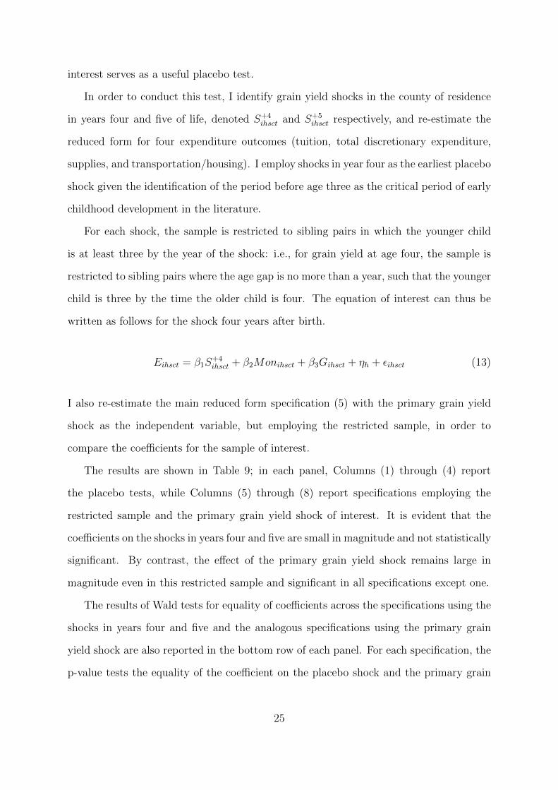
In order to conduct this test, I identify grain yield shocks in the county of residence

in years four and five of life, denoted S+4ihsct and S+5

ihsct respectively, and re-estimate the

reduced form for four expenditure outcomes (tuition, total discretionary expenditure,

supplies, and transportation/housing). I employ shocks in year four as the earliest placebo

shock given the identification of the period before age three as the critical period of early

childhood development in the literature.

For each shock, the sample is restricted to sibling pairs in which the younger child

is at least three by the year of the shock: i.e., for grain yield at age four, the sample is

restricted to sibling pairs where the age gap is no more than a year, such that the younger

child is three by the time the older child is four. The equation of interest can thus be

written as follows for the shock four years after birth.

Eihsct = β1S+4ihsct + β2Monihsct + β3Gihsct + ηh + εihsct (13)

I also re-estimate the main reduced form specification (5) with the primary grain yield

shock as the independent variable, but employing the restricted sample, in order to

compare the coefficients for the sample of interest.

The results are shown in Table 9; in each panel, Columns (1) through (4) report

the placebo tests, while Columns (5) through (8) report specifications employing the

restricted sample and the primary grain yield shock of interest. It is evident that the

coefficients on the shocks in years four and five are small in magnitude and not statistically

significant. By contrast, the effect of the primary grain yield shock remains large in

magnitude even in this restricted sample and significant in all specifications except one.

The results of Wald tests for equality of coefficients across the specifications using the

shocks in years four and five and the analogous specifications using the primary grain

yield shock are also reported in the bottom row of each panel. For each specification, the

p-value tests the equality of the coefficient on the placebo shock and the primary grain

25

yield shock using the same sample; for example, the p-value in Column (1) of Panel A

tests equality of the coefficients across Columns (1) and (5) of that panel. For the year

four shocks, equality of the coefficients can be rejected for two of the four measures of

expenditure, and for the third the specification narrowly fails to reject at the 10 percent

level. For the year five shocks, equality of the coefficient in the placebo test and the

primary coefficient of interest can be rejected for all four measures of expenditure. This

evidence suggests that climatic shocks later in childhood do not significantly determine

parental allocation of educational expenditure, consistent with the assumption that the

channel of causality for the primary results runs through the effect of climatic shocks on

child development during a critical period in infancy.

5 Conclusion

In the previous literature on intrahousehold allocation, the question of the presence or

absence of family aversion to inequality has received extensive analytical attention. How-

ever, little evidence has been presented regarding the nature of parental responses to

systematic differences in endowment among children, particularly among non-twins.

Employing an identification strategy that relies on the correlation between climatic

variation and children’s endowment, mediated through the impact of nutritional shocks

in infancy, I find a pattern of preferential allocations of discretionary educational ex-

penditure to children of lower endowment. This is consistent with a parental preference

for equality of outcomes. The relationship is robust across multiple specifications and

measures of expenditure, and robust to the inclusion of both gender and sibling parity.

These results imply that, at least in education, the household is serving as a mechanism

for the mitigation of existing inequalities. There is, however, no evidence that health

expenditure follows a similar pattern.

These results raise the question of whether the observed allocation favoring the weaker

child is a compensatory response intended to provide consumption-like educational ben-

26

efits to children with lower endowments, or whether this allocation strategy reflects dif-

ferential returns to educational expenditure for children of differing levels of endowment.

If, for example, educational expenditure has higher returns for the child with a lower en-

dowment - or more accurately, is perceived by parents to have higher returns - then the

observed strategy could be interpreted as maximizing returns to educational investment.

While no robust evidence on this point is available in this sample, a survey of the

mothers of the sampled children does collect information on the level of education she

expects each of the sampled children to attain. A simple test of the perceptions of the

returns to educational expenditure on different children can be implemented by regressing

this expectation on reported expenditure, height-for-age and the interaction between the

two conditional on household fixed effects, instrumenting for height-for-age with grain

yield in infancy. This test shows no evidence that returns to expenditure are perceived by

mothers to be systematically different for children of varying height-for-age.11 While this

evidence must be considered to be only suggestive, it is consistent with parents seeking

to provide a consumption-like benefit to children of lower initial endowment, rather than

responding to systematic differences in returns to expenditure across different children.

For the purposes of the welfare analysis of potential household interventions, this is an

encouraging result that suggests that household-level interventions may improve welfare

outcomes for the weakest members of a family. Policy interventions that aim to increase

human capital investment for struggling children are typically targeted at a household

level. Even if a transfer is specifically designated for a particular child, this provision is

challenging to observe or enforce, and parental reallocation of other consumption may

undo any intended benefit for the child of interest. Accordingly, evidence that household

processes of allocation in the rural Chinese context favor the direction of human capital

resources toward children that have experienced negative shocks and the associated neg-

ative health effects may provide a higher degree of confidence that external transfers to

these households will in fact benefit their more vulnerable children.

11Tabulations available on request.

27

References

Alderman, Harold, John Hoddinott, and Bill Kinsey, “Long-term consequences

of early childhood malnutrition,” Oxford Economic Papers, 2006, 58 (3), 450–474.

Almond, Douglas, “Is the 1918 influenza pandemic over? Long-term effects of in-utero

influenza exposure in the post-1940 U.S. population,” Journal of Political Economy,

2006, 114, 612712.

and Kenneth Chay, “The long-run and intergenerational impact of poor infant

health: Evidence from cohorts born during the Civil Rights era,” 2006.

, Lena Edlund, Hongbin Li, and Jushen Zhang, “Long-term effects of the 1959-

1961 China famine: Mainland China and Hong Kong,” 2006.

Banerjee, Abhijit, Esther Duflo, Gilles Postel-Vinay, and Tim Watts, “Long-run

health impacts of income shocks: Wine and phylloxera in nineteenth-century France,”

Review of Economics and Statistics, 2010, 92, 714–728.

Banister, Judith, “Shortage of girls in China today,” Journal of Population Research,

2004, 21 (1), 19–45.

Behrman, Jere, “Intrahousehold allocation of nutrients in rural India: Are boys fa-

vored? Do parents exhibit inequality aversion?,” Oxford Economic Papers, 1988, 40,

32–54.

and Anil Deolalikar, “Intrahousehold demand for nutrients in rural South India: in-

dividual estimates, fixed effects and permanent income,” Journal of Human Resources,

1990, 25 (4), 665–696.

, Robert Pollak, and Paul Taubman, “Parental preferences and provision for

progeny,” Journal of Political Economy, 1982, 90 (1), 52–73.

28

Bommiere, Antoine and Sylvie Lambert, “Human capital investments and family

composition,” Applied Economics Letters, 2004, 11 (3), 193–196.

Butcher, Kristin F. and Anne Case, “The effect of sibling sex composition on

women’s education and earnings,” The Quarterly Journal of Economics, August 1994,

109 (3), 531–563.

Coale, Ansley and Judith Banister, “Five decades of missing females in China,”

Demography, August 1994, 31 (3).

Conti, Gabriella, James J. Heckman, Junjian Yi, and Junsen Zhang, “Early

health shocks, parental responses and child outcomes,” 2010.

Garg, Ashish and Jonathan Morduch, “Sibling rivalry and the gender gap: evidence

from child health outcomes in Ghana,” Journal of Population Economics, December

1998, 11 (4), 1432–1475.

Grantham-McGregor, Sally and Cornelius Ani, “A review of studies on the effect

of iron deficiency on cognitive development in children,” Journal of Nutrition, 2001,

131, 649S–668.

, Yin Bun Cheung, Santiago Cueto, Paul Glewwe, Linda Richter, and Bar-

bara Strupp, “Development potential for children in the first five years in developing

countries,” The Lancet, Jan. 2007, 369 (9555), 60–70.

Griliches, Zvi, “Sibling models and data in economics: beginnings of a survey,” Journal

of Political Economy, 1979, 87 (5), S37–S64.

Gu, Baochang, Wang Feng, Guo Zhigang, and Zhang Erli, “China’s local and

national fertility policies at the end of the twentieth century,” Population and Devel-

opment Review, 2007, 33, 129–147.

Hazarika, Gautam, “Gender differences in children’s nutrition and access to health

care,” Journal of Development Studies, 2000, 37 (1), 73–92.

29

Leenstra, T., L.T. Petersen, S.K. Kariuki, A.J. Oloo, P.A. Kager, and F.O. ter

Kuile, “Prevalence and severity of malnutrition and age at menarche; cross-sectional

studies in adolescent schoolgirls in western Kenya,” American Journal of Clinical Nu-

trition, 2005, 59 (S2), 41–48.

Maccini, Sharon and Dean Yang, “Under the weather: Health, schooling and eco-

nomic consequences of early-life rainfall,” American Economic Review, 2009, 99 (3),

1006–1026.

Martorell, Reynaldo, “The nature of child malnutrition and its long-term implica-

tions,” Food and Nutrition Bulletin, 1999, 20, 288–292.

Meng, Xin and Nancy Qian, “The long term consequences of famine on survivors:

Evidence from a unique natural experiment using China’s Great Famine,” 2009.

Morduch, Jonathan, “Sibling rivalry in Africa,” American Economic Review, May

2000, 90 (2), 405–409.

Ono, Hiroshi, “Are sons and daughters substitutable? Allocation of family resources

in contemporary Japan,” Journal of the Japanese and International Economies, June

2004, 18, 143–160.

Parish, William L. and Robert Willis, “Daughters, education and family budgets:

Taiwan Experiences,” The Jouanl of Human Resources, Autumn 1993, 28 (24), 863–

898.

Pollitt, Ernesto, Kathleen S. Gorman, Patrice L. Engle, Juan A. Rivera, and

Reynaldo Martorell, “Nutrition in Early Life and the Fulfillment of Intellectual

Potential,” Journal of Nutrition, 1999, 125, 1111S–1118.

Prista, Antonio, Jose Antonio Ribeiro Maia, Albertino Damasceno, and Gas-

ton Beunen, “Anthropometric indicators of nutritional status: implications for fitness,

30

activity and health in school-age children and adolescents from Maputo, Mozambique,”

American Journal of Clinical Nutrition, 2003, 77 (4), 952–959.

Qian, Zhenchao, “Progression to second birth in China: a study of four rural counties,”

Population Studies, Jul. 1997, 51 (2), 221–229.

Rosenzweig, Mark and Junsen Zhang, “Do population control policies induce more

human capital investment? Twins, birth weight and China’s ’one-child policy,” The

Review of Economic Studies, 2009, 76, 1149–1174.

and Kenneth Wolpin, “Heterogeneity, intrafamily distribution and child health,”

Journal of Human Resources, 1988, 23 (4), 427–461.

Sawaya, Ana, Gerald Dallal, Gisela Solymos, Maria de Sousa, Maria Ventura,

Susan Roberts, and Dirce Sigulem, “Obesity and malnutrition in a shantytown

population in the city of Sao Paulo, Brazil,” Obesity Research, 1995, 3 (S2), 107s–115s.

Strauss, John and Duncan Thomas, “Human resources: Empirical modeling of

household and family decisions,” in J. Behrman and T.N. Srinavasan, eds., Handbook

of Development Economics, North-Holland: Elsevier Science, 1995.

Tenikue, Michel and Bertrand Verheyden, “Birth Order, Child Labor and School-

ing: Theory and Evidence from Cameroon,” 2007.

Trias, Julieta, “The positive impact of negative shocks: Infant mortality and agricul-

tural productivity shocks,” 2013.

World Health Organization, “An evaluation of infant growth: the use and interpre-

tation of anthropometry in infants,” Bulletin of the World Health Organization, 1995,

73, 163–74.

31

6 Tables

Table 1: Summary statistics

Panel A: Demographic data Panel B: Educational expenditure per child

Sample Subsample p-value Mean Std. Dev. Max.Net income 6791.97 6169.01 .352 Total 260.27 311.48 4240Net income agri. 2618.84 2444.59 .276 Discretionary 97.88 181.11 2240Income per capita 1705.01 1525.74 .234 Tuition 162.4 170.08 2000Father educ. 7.11 6.88 .142 Supplies 35.67 38.26 300Mother educ. 4.29 4.1 .199 Transport/Housing 11.81 45.66 600Father age 42.62 38.95 .061 Food 35.5 115.02 1700Mother age 39.25 36.88 0 Tutoring 5.41 16.02 100Index child age 15.1 15.01 .081 Other fees 9.49 27.73 360Height-for-age -1.19 -1.31 .017

Obs. 1918 413

Notes: The sample encompasses the full sample of households that report income data; this is 1918 out of the full sampleof 2000 households in the survey. The subsample is households with two-children families in which both children reportanthropometric data. There are 413 households in the subsample of interest, and 826 children. Income is reported inyuan; educational expenditure is reported in yuan per semester. Column (3) reports the p-value for a test of equality ofmeans across the sample and subsample.

Table 2: OLS

Enrollment Total Discretionary Tuition Supplies Trans./Housing Food Tutoring Other(1) (2) (3) (4) (5) (6) (7) (8) (9)

Height-for-age .009 -7.259 -6.676 -.584 -1.897 -.503 -4.473 .715 -.519(.009) (11.079) (7.254) (7.135) (1.016)∗ (1.246) (5.938) (.502) (.708)

Mean (levels) .95 260.27 97.88 162.4 35.67 11.81 35.5 5.41 9.49Median (levels) 1 180 40 125 25 0 0 0 0Mean (dif.) -.07 -145.06 -79.15 -65.9 -13.37 -14.16 -39.78 -5.58 -6.26Obs. 826 826 826 826 826 826 826 826 826

Notes: The dependent variable is educational expenditure on a given child in the specified category; the independentvariable is height-for-age. All regressions include household fixed effects and standard errors clustered by county. Themean in differences reports the mean intra-household difference in expenditure (between the first and second child) in thespecified category. Asterisks denote significance at the 1, 5, and 10 percent levels.

32

Tab

le3:

Fir

stst

age

(1)

(2)

(3)

(4)

(5)

(6)

(7)

(8)

(9)

PanelA:Cro

ss-h

ousehold

variation

inheight-for-age

Ute

rosh

ock

.138

.131

.139

(.039)∗

∗∗(.

043)∗

∗∗(.

047)∗

∗∗

Yea

r1

shock

.130

.117

.136

(.040)∗

∗∗(.

046)∗

∗(.

044)∗

∗∗

Yea

r2

shock

.134

.134

.131

(.035)∗

∗∗(.

040)∗

∗∗(.

042)∗

∗∗

Sam

ple

All

Fir

st-b

orn

Sec

ond

-born

All

Fir

st-b

orn

Sec

on

d-b

orn

All

Fir

st-b

orn

Sec

on

d-b

orn

Ob

s.82

240

941

3826

413

413

822

409

413

F12

.586

3.54

86.

99

13.5

13.2

36.9

62

15.4

06

4.3

37

7.1

91

PanelB:W

ithin-h

ousehold

variation

inheight-for-age

Ute

rosh

ock

.537

.554

(.175)∗

∗∗(.

188)∗

∗∗

Yea

r1

shock

.513

.531

(.164)∗

∗∗(.

178)∗

∗∗

Yea

r2

shock

.430

.443

(.149)∗

∗∗(.

196)∗

∗

Tot

alsh

ock

.579

.496

.410

(.176)∗

∗∗(.

151)∗

∗∗(.

137)∗

∗∗

Mon

thin

t.-.

002

(.009)

Mon

thin

t.-.

002

(.008)

Mon

thin

t.-.

001

(.009)

Sib

lin

gsh

ock

-.156

(.130)

Fix

edeff

ects

Hou

seh

old

Hou

seh

old

Hou

seh

old

Hou

seh

old

Hou

seh

old

Hou

seh

old

Hou

seh

old

Cou

nty

an

del

der

year-

of-

bir

thO

bs.

822

826

822

826

822

826

822

826

826

F4.

409

4.61

23.

927

5.1

37

2.2

23

2.3

06

2.2

9.9

08

5.1

6

Note

s:T

he

dep

end

ent

vari

able

ish

eight-

for-

age;

the

ind

epen

den

tvari

ab

les

are

gra

inyie

ldin

the

spec

ified

yea

r,m

onth

of

bir

th,

inte

ract

ion

sb

etw

een

month

of

bir

than

dgra

inyie

ldsh

ock

s,an

dgra

inyie

ldin

the

sib

lin

g’s

yea

rof

bir

th.

Th

esa

mp

leem

plo

yed

an

dfi

xed

effec

tsin

clu

ded

are

spec

ified

inth

eta

ble

;st

an

dard

erro

rsare

clu

ster

edby

cou

nty

.A

ster

isks

den

ote

sign

ifica

nce

at

the

1,

5,

an

d10

per

cent

level

s.

33

Tab

le4:

Red

uce

dfo

rman

dtw

o-st

age

leas

tsq

uar

es

En

roll

.T

otal

Dis

cret

.T

uit

ion

Su

pp

lies

Tra

nsp

ort

ati

on

/H

ou

sin

gF

ood

Tu

tori

ng

Oth

er(1

)(2

)(3

)(4

)(5

)(6

)(7

)(8

)(9

)

PanelA:Reduced

form

Gra

inyie

ld-.

055

-288

.166

-207.7

86

-80.3

80

-21.4

23

-35.6

43

-121.8

39

-12.1

65

-16.7

16

(.035)

(34.3

16)∗

∗∗(3

2.7

31)∗

∗∗(1

6.9

21)∗

∗∗(3

.522)∗

∗∗(6

.077)∗

∗∗(2

5.5

09)∗

∗∗(2

.260)∗

∗∗(3

.251)∗

∗∗

Gra

inyie

ld-.

322

-.307

-.206

-.085

(.036)∗

∗∗(.

053)∗

∗∗(.

022)∗

∗∗(.

035)∗

∗

Pri

mar

ysp

ec.

+sc

hool

contr

ols

-.01

9-1

99.8

51

-159.2

03

-40.6

48

-10.4

12

-29.9

24

-98.6

13

-8.8

14

-11.4

40

(.032)

(39.3

80)∗

∗∗(3

2.7

17)∗

∗∗(1

6.2

95)∗

∗(3

.158)∗

∗∗(7

.529)∗

∗∗(2

5.5

11)∗

∗∗(2

.069)∗

∗∗(3

.519)∗

∗∗

Pri

mar

ysp

ec.

+gr

ade

leve

l-.

083

-109

.839

-129.5

83

19.7

44

-3.9

06

-21.6

69

-84.9

02

-8.1

89

-10.9

17

(.049)∗

(43.5

31)∗

∗(3

9.4

21)∗

∗∗(1

3.3

40)

(4.9

14)

(5.9

39)∗

∗∗(2

8.0

81)∗

∗∗(2

.638)∗

∗∗(4

.781)∗

∗

PanelB:Two-sta

geleast

square

s

Hei

ght-

for-

age

-.09

6-4

97.5

01

-358.7

30

-138.7

72

-36.9

85

-61.5

35

-210.3

48

-21.0

02

-28.8

60

(.065)

(157.1

07)∗

∗∗(1

24.4

01)∗

∗∗(4

4.8

10)∗

∗∗(1

0.3

64)∗

∗∗(2

1.5

81)∗

∗∗(7

9.8

20)∗

∗∗(7

.718)∗

∗∗(1

1.3

53)∗

∗

An

der

son

-Ru

bin

p-v

alu

e.2

09.0

37.0

00

.062

.422

.065

.013

.004

Hei

ght-

for-

age

-.555

-.530

-.356

-.146

(.179)∗

∗∗(.

180)∗

∗∗(.

118)∗

∗∗(.

087)∗

Pri

mar

ysp

ec.

+sc

hool

contr

ols

-.03

4-3

50.7

93

-279.4

45

-71.3

48

-18.2

76

-52.5

25

-173.0

93

-15.4

71

-20.0

80

(.057)

(124.2

96)∗

∗∗(1

03.0

37)∗

∗∗(3

3.4

66)∗

∗(6

.877)∗

∗∗(2

0.9

75)∗

∗(6

8.8

36)∗

∗(6

.168)∗

∗(9

.751)∗

∗

Pri

mar

ysp

ec.

+gr

ade

leve

l-.

151

-199

.936

-235.8

75

35.9

40

-7.1

10

-39.4

44

-154.5

44

-14.9

06

-19.8

71

(.095)

(90.5

30)∗

∗(8

7.0

91)∗

∗∗(2

4.8

23)

(9.0

86)

(13.9

91)∗

∗∗(5

8.8

07)∗

∗∗(5

.794)∗

∗(1

0.5

50)∗

Mea

n(l

evel

s).9

526

0.27

97.8

8162.4

35.6

711.8

135.5

5.4

19.4

9M

edia

n(l

evel

s)1

180

40

125

25

00

00

Mea

n(d

iffer

ence

s)-.

07-1

45.0

6-7

9.1

5-6

5.9

-13.3

7-1

4.1

6-3

9.7

8-5

.58

-6.2

6O

bs.

826

826

826

826

826

826

826

826

826

Note

s:T

he

dep

end

ent

vari

able

ised

uca

tion

al

exp

end

itu

reon

agiv

ench

ild

inth

esp

ecifi

edca

tegory

;th

esa

mp

leis

child

ren

livin

gin

two-c

hild

ren

hou

seh

old

s.In

Pan

elA

,th

ein

dep

end

ent

vari

ab

leis

the

mea

nof

rep

ort

edgra

inyie

ldin

ute

roan

din

the

firs

tan

dse

con

dyea

rsof

life

;in

Pan

elB

,th

ein

dep

end

ent

vari

ab

leis

hei

ght-

for-

age

inst

rum

ente

dby

this

gra

inyie

ldvari

ab

le.

All

regre

ssio

ns

incl

ud

eh

ou

seh

old

fixed

effec

tsan

dst

an

dard

erro

rscl

ust

ered

by

cou

nty

.S

chool-

level

contr

ols

incl

ud

edare

the

typ

eof

sch

ool

(pri

mary

,m

idd

leor

hig

h),

wh

eth

erth

esc

hool

isp

ub

lic

or

pri

vate

,th

enu

mb

erof

class

esp

erd

ay,

the

nu

mb

erof

wee

ks

inth

esc

hool

yea

r,th

enu

mb

erof

board

ing

stu

den

tsat

the

sch

ool,

the

tota

lnu

mb

erof

stu

den

tsre

port

edin

the

sch

ool,

the

per

centa

ge

wit

hru

ral

regis

trati

on

(hu

kou

),th

ep

erce

nta

ge

wh

oare

eth

nic

min

ori

ties

,th

ep

erce

nta

ge

of

stu

den

tsab

sent

from

sch

ool

on

the

pre

ced

ing

day,

an

dth

enu

mb

erof

teach

ers;

all

sch

ool

chara

cter

isti

csare

rep

ort

edby

the

pri

nci

pal.

Th

em

ean

ind

iffer

ence

sre

port

sth

em

ean

intr

a-h

ou

seh

old

diff

eren

cein

exp

end

itu

re(b

etw

een

the

firs

tan

dse

con

dch

ild

)in

the

spec

ified

cate

gory

.T

he

An

der

son

-Ru

bin

p-v

alu

eis

rep

ort

edfo

rth

eb

ase

two-s

tage

least

squ

are

ssp

ecifi

cati

on

,in

clu

din

gn

oad

dit

ion

al

contr

ols

.A

ster

isks

den

ote

sign

ifica

nce

at

the

1,

5,

an

d10

per

cent

level

s.

34

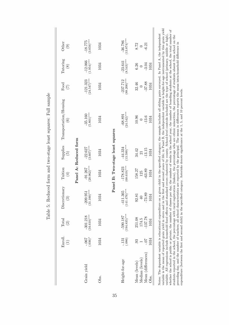
Tab

le5:

Red

uce

dfo

rman

dtw

o-st

age

leas

tsq

uar

es:

Full

sam

ple

En

roll

.T

otal

Dis

cret

ion

ary

Tu

itio

nS

up

pli

esT

ran

sport

ati

on

/H

ou

sin

gF

ood

Tu

tori

ng

Oth

er(1

)(2

)(3

)(4

)(5

)(6

)(7

)(8

)(9

)

PanelA:Reduced

form

Gra

inyie

ld-.

067

-301

.218

-209

.951

-91.2

67

-22.6

27

-35.1

60

-121.3

23

-12.0

66

-18.7

75

(.036)∗

(34.6

10)∗

∗∗(3

1.1

00)∗

∗∗(2

0.9

62)∗

∗∗(3

.607)∗

∗∗(5

.801)∗

∗∗(2

4.5

47)∗

∗∗(1

.954)∗

∗∗(3

.059)∗

∗∗

Ob

s.10

3410

3410

34

1034

1034

1034

1034

1034

1034

PanelB:Two-sta

geleast

square

s

Hei

ght-

for-

age

-.13

1-5

90.1

87-4

11.3

65

-178.8

23

-44.3

34

-68.8

91

-237.7

12

-23.6

41

-36.7

86

(.086)

(194.8

35)∗

∗∗(1

41.4

76)∗

∗∗(6

8.6

19)∗

∗∗(1

3.5

99)∗

∗∗(2

4.5

42)∗

∗∗(8

8.2

00)∗

∗∗(8

.543)∗

∗∗(1

3.8

74)∗

∗∗

Mea

n(l

evel

s).9

325

1.08

92.8

1158.2

734.4

210.9

632.4

66.2

68.7

2M

edia

n(l

evel

s)1

174.

540

125

21

00

00

Mea

n(d

iffer

ence

s)-.

07-1

37.7

8-7

3.89

-63.8

9-1

3.1

5-1

3.6

-37.8

8-3

.04

-6.2

1O

bs.

1034

1034

1034

1034

1034

1034

1034

1034

Note

s:T

he

dep

end

ent

vari

able

ised

uca

tion

al

exp

end

itu

reon

agiv

ench

ild

inth

esp

ecifi

edca

tegory

;th

esa

mp

lein

clu

des

all

sib

lin

gp

air

ssu

rvey

ed.

InP

an

elA

,th

ein

dep

end

ent

vari

ab

leis

the

mea

nof

rep

ort

edgra

inyie

ldin

ute

roan

din

the

firs

tan

dse

con

dyea

rsof

life

;in

Pan

elB

,th

ein

dep

end

ent

vari

ab

leis

hei

ght-

for-

age

inst

rum

ente

dby

this

gra

inyie

ldvari

ab

le.

All

regre

ssio

ns

incl

ud

eh

ou

seh

old

fixed

effec

tsan

dst

an

dard

erro

rscl

ust

ered

by

cou

nty

.S

chool-

level

contr

ols

incl

ud

edare

the

typ

eof

sch

ool

(pri

mary

,m

idd

leor

hig

h),

wh

eth

erth

esc

hool

isp

ub

lic

or

pri

vate

,th

enu

mb

erof

class

esp

erd

ay,

the

nu

mb

erof

wee

ks

inth

esc

hool

yea

r,th

enu

mb

erof

board

ing

stu

den

tsat

the

sch

ool,

the

tota

lnu

mb

erof

stu

den

tsre

port

edin

the

sch

ool,

the

per

centa

ge

wit

hru

ral

regis

trati

on

(hu

kou

),th

ep

erce

nta

ge

wh

oare

eth

nic

min

ori

ties

,th

ep

erce

nta

ge

of

stu

den

tsab

sent

from

sch

ool

on

the

pre

ced

ing

day,

an

dth

enu

mb

erof

teach

ers;

all

sch

ool

chara

cter

isti

csare

rep

ort

edby

the

pri

nci

pal.

Th

em

ean

ind

iffer

ence

sre

port

sth

em

ean

intr

a-h

ou

seh

old

diff

eren

cein

exp

end

itu

re(b

etw

een

the

firs

tan

dse

con

dch

ild

)in

the

spec

ified

cate

gory

.A

ster

isks

den

ote

sign

ifica

nce

at

the

1,

5,

an

d10

per

cent

level

s.

35

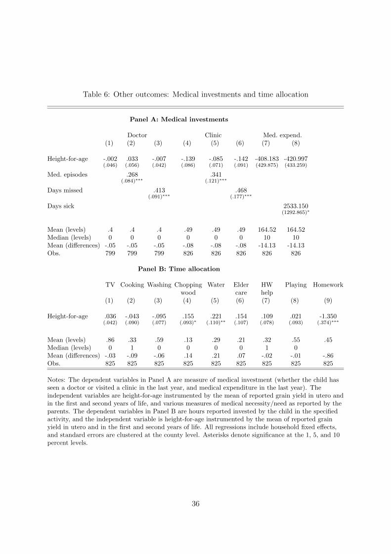
Table 6: Other outcomes: Medical investments and time allocation

Panel A: Medical investments

Doctor Clinic Med. expend.(1) (2) (3) (4) (5) (6) (7) (8)

Height-for-age -.002 .033 -.007 -.139 -.085 -.142 -408.183 -420.997(.046) (.056) (.042) (.086) (.071) (.091) (429.875) (433.259)

Med. episodes .268 .341(.084)∗∗∗ (.121)∗∗∗

Days missed .413 .468(.091)∗∗∗ (.177)∗∗∗

Days sick 2533.150(1292.865)∗

Mean (levels) .4 .4 .4 .49 .49 .49 164.52 164.52Median (levels) 0 0 0 0 0 0 10 10Mean (differences) -.05 -.05 -.05 -.08 -.08 -.08 -14.13 -14.13Obs. 799 799 799 826 826 826 826 826

Panel B: Time allocation

TV Cooking Washing Chopping Water Elder HW Playing Homeworkwood care help

(1) (2) (3) (4) (5) (6) (7) (8) (9)

Height-for-age .036 -.043 -.095 .155 .221 .154 .109 .021 -1.350(.042) (.090) (.077) (.093)∗ (.110)∗∗ (.107) (.078) (.093) (.374)∗∗∗

Mean (levels) .86 .33 .59 .13 .29 .21 .32 .55 .45Median (levels) 0 1 0 0 0 0 1 0Mean (differences) -.03 -.09 -.06 .14 .21 .07 -.02 -.01 -.86Obs. 825 825 825 825 825 825 825 825 825

Notes: The dependent variables in Panel A are measure of medical investment (whether the child hasseen a doctor or visited a clinic in the last year, and medical expenditure in the last year). Theindependent variables are height-for-age instrumented by the mean of reported grain yield in utero andin the first and second years of life, and various measures of medical necessity/need as reported by theparents. The dependent variables in Panel B are hours reported invested by the child in the specifiedactivity, and the independent variable is height-for-age instrumented by the mean of reported grainyield in utero and in the first and second years of life. All regressions include household fixed effects,and standard errors are clustered at the county level. Asterisks denote significance at the 1, 5, and 10percent levels.

36

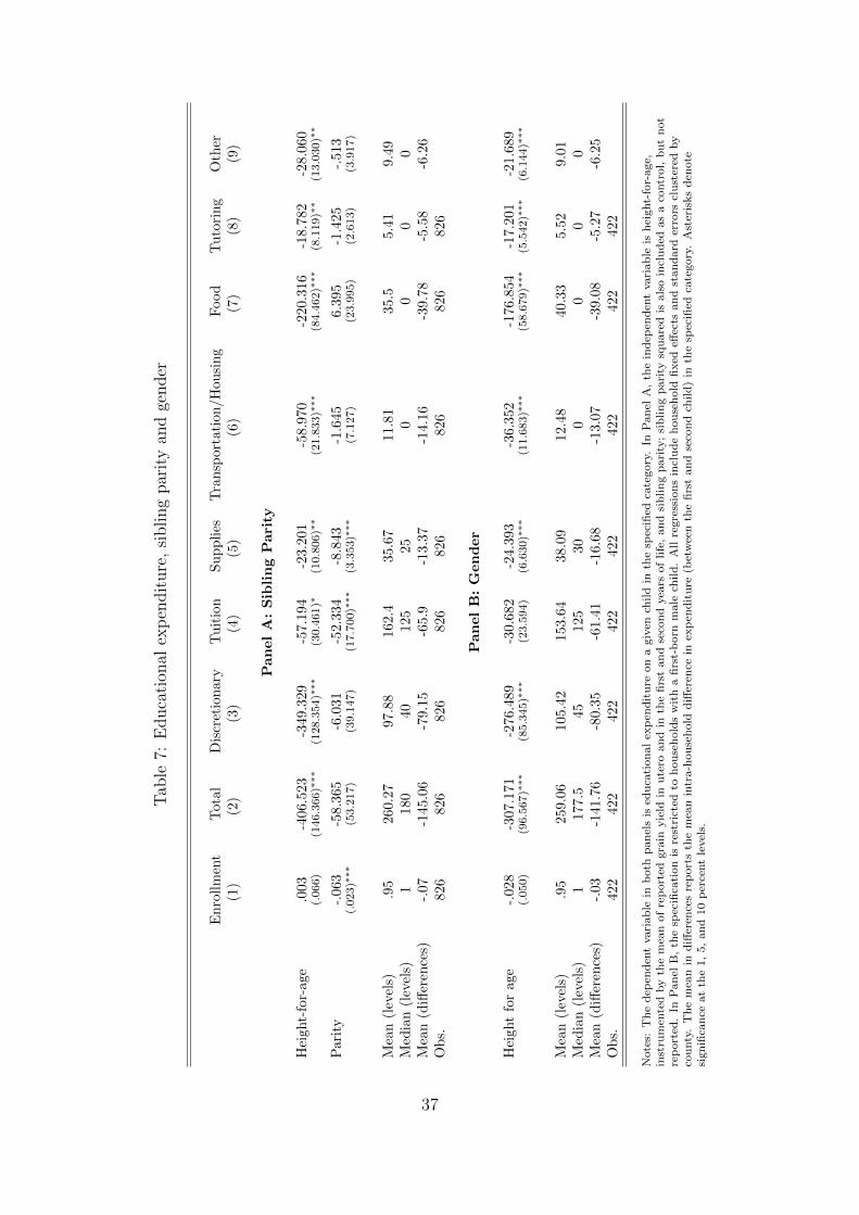
Tab

le7:

Educa

tion

alex

pen

dit

ure

,si

bling

par

ity

and

gender

En

roll

men

tT

otal

Dis

cret

ion

ary

Tu

itio

nS

up

pli

esT

ran

sport

ati

on

/H

ou

sin

gF

ood

Tu

tori

ng

Oth

er(1

)(2

)(3

)(4

)(5

)(6

)(7

)(8

)(9

)

PanelA:SiblingParity

Hei

ght-

for-

age

.003

-406

.523

-349.3

29

-57.1

94

-23.2

01

-58.9

70

-220.3

16

-18.7

82

-28.0

60

(.066)

(146.3

66)∗

∗∗(1

28.3

54)∗

∗∗(3

0.4

61)∗

(10.8

06)∗

∗(2

1.8

33)∗

∗∗(8

4.4

62)∗

∗∗(8

.119)∗

∗(1

3.0

30)∗

∗

Par

ity

-.06

3-5

8.36

5-6

.031

-52.3

34

-8.8

43

-1.6

45

6.3

95

-1.4

25

-.513

(.023)∗

∗∗(5

3.2

17)

(39.1

47)

(17.7

00)∗

∗∗(3

.353)∗

∗∗(7

.127)

(23.9

95)

(2.6

13)

(3.9

17)

Mea

n(l

evel

s).9

526

0.27

97.8

8162.4

35.6

711.8

135.5

5.4

19.4

9M

edia

n(l

evel

s)1

180

40

125

25

00

00

Mea

n(d

iffer

ence

s)-.

07-1

45.0

6-7

9.1

5-6

5.9

-13.3

7-1

4.1

6-3

9.7

8-5

.58

-6.2

6O

bs.

826

826

826

826

826

826

826

826

PanelB:Gender

Hei

ght

for

age

-.02

8-3

07.1

71-2

76.4

89

-30.6

82

-24.3

93

-36.3

52

-176.8

54

-17.2

01

-21.6

89

(.050)

(96.5

67)∗

∗∗(8

5.3

45)∗

∗∗(2

3.5

94)

(6.6

30)∗

∗∗(1

1.6

83)∗

∗∗(5

8.6

79)∗

∗∗(5

.542)∗

∗∗(6

.144)∗

∗∗

Mea

n(l

evel

s).9

525

9.06

105.4

2153.6

438.0

912.4

840.3

35.5

29.0

1M

edia

n(l

evel

s)1

177.

545

125

30

00

00

Mea

n(d

iffer

ence

s)-.

03-1

41.7

6-8

0.3

5-6

1.4

1-1

6.6

8-1

3.0

7-3

9.0

8-5

.27

-6.2

5O

bs.

422

422

422

422

422

422

422

422

Note

s:T

he

dep

end

ent

vari

able

inb

oth

pan

els

ised

uca

tion

al

exp

end

itu

reon

agiv

ench

ild

inth

esp

ecifi

edca

tegory

.In

Pan

elA

,th

ein

dep

end

ent

vari

ab

leis

hei

ght-

for-

age,

inst

rum

ente

dby

the

mea

nof

rep

ort

edgra

inyie

ldin

ute

roan

din

the

firs

tan

dse

con

dyea

rsof

life

,an

dsi

blin

gp

ari

ty;

sib

lin

gp

ari

tysq

uare

dis

als

oin

clu

ded

as

aco

ntr

ol,

bu

tn

ot

rep

ort

ed.

InP

an

elB

,th

esp

ecifi

cati

on

isre

stri

cted

toh

ou

seh

old

sw

ith

afi

rst-

born

male

child

.A

llre

gre

ssio

ns

incl

ud

eh

ou

seh

old

fixed

effec

tsan

dst

an

dard

erro

rscl

ust

ered

by

cou

nty

.T

he

mea

nin

diff

eren

ces

rep

ort

sth

em

ean

intr

a-h

ou

seh

old

diff

eren

cein

exp

end

itu

re(b

etw

een

the

firs

tan

dse

con

dch

ild

)in

the

spec

ified

cate

gory

.A

ster

isks

den

ote

sign

ifica

nce

at

the

1,

5,

an

d10

per

cent

level

s.

37

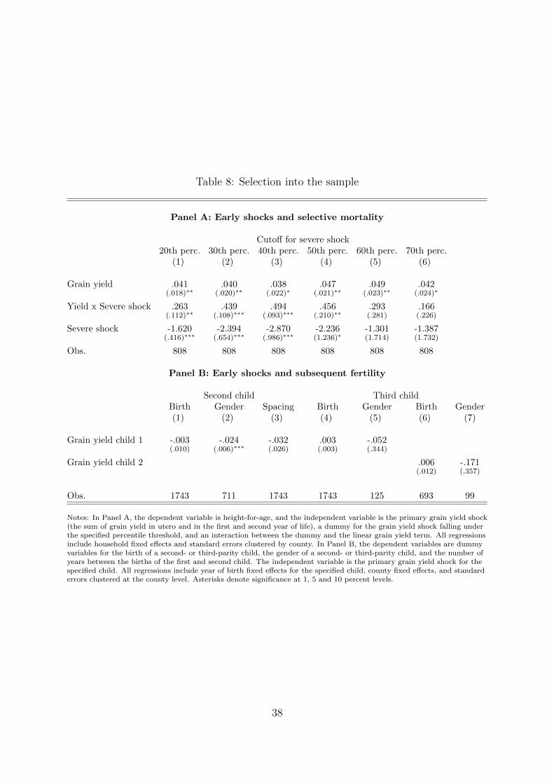
Table 8: Selection into the sample

Panel A: Early shocks and selective mortality

Cutoff for severe shock20th perc. 30th perc. 40th perc. 50th perc. 60th perc. 70th perc.

(1) (2) (3) (4) (5) (6)

Grain yield .041 .040 .038 .047 .049 .042(.018)∗∗ (.020)∗∗ (.022)∗ (.021)∗∗ (.023)∗∗ (.024)∗

Yield x Severe shock .263 .439 .494 .456 .293 .166(.112)∗∗ (.108)∗∗∗ (.093)∗∗∗ (.210)∗∗ (.281) (.226)

Severe shock -1.620 -2.394 -2.870 -2.236 -1.301 -1.387(.416)∗∗∗ (.654)∗∗∗ (.986)∗∗∗ (1.236)∗ (1.714) (1.732)

Obs. 808 808 808 808 808 808

Panel B: Early shocks and subsequent fertility

Second child Third childBirth Gender Spacing Birth Gender Birth Gender(1) (2) (3) (4) (5) (6) (7)

Grain yield child 1 -.003 -.024 -.032 .003 -.052(.010) (.006)∗∗∗ (.026) (.003) (.344)

Grain yield child 2 .006 -.171(.012) (.357)

Obs. 1743 711 1743 1743 125 693 99

Notes: In Panel A, the dependent variable is height-for-age, and the independent variable is the primary grain yield shock(the sum of grain yield in utero and in the first and second year of life), a dummy for the grain yield shock falling underthe specified percentile threshold, and an interaction between the dummy and the linear grain yield term. All regressionsinclude household fixed effects and standard errors clustered by county. In Panel B, the dependent variables are dummyvariables for the birth of a second- or third-parity child, the gender of a second- or third-parity child, and the number ofyears between the births of the first and second child. The independent variable is the primary grain yield shock for thespecified child. All regressions include year of birth fixed effects for the specified child, county fixed effects, and standarderrors clustered at the county level. Asterisks denote significance at 1, 5 and 10 percent levels.

38

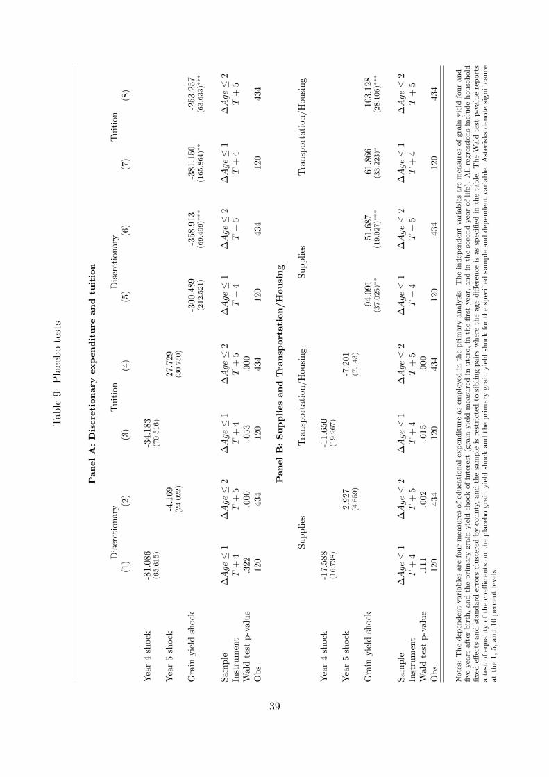
Tab

le9:

Pla

ceb

ote

sts

PanelA:Discre

tionary

expenditure

and

tuition

Dis

cret

ion

ary

Tu

itio

nD

iscr

etio

nary

Tu

itio

n(1

)(2

)(3

)(4

)(5

)(6

)(7

)(8

)

Yea

r4

shock

-81.

086

-34.1

83

(65.6

15)

(70.5

16)

Yea

r5

shock

-4.1

6927.7

29

(24.0

22)

(30.7

50)

Gra

inyie

ldsh

ock

-300.4

89

-358.9

13

-381.1

50

-253.2

57

(212.5

21)

(69.4

99)∗

∗∗(1

65.8

64)∗

∗(6

3.6

33)∗

∗∗

Sam

ple

∆Age≤

1∆Age≤

2∆Age≤

1∆Age≤

2∆Age≤

1∆Age≤

2∆Age≤

1∆Age≤

2In

stru

men

tT

+4

T+

5T

+4

T+

5T

+4

T+

5T

+4

T+

5W

ald

test

p-v

alu

e.3

22.0

00.0

53

.000

Ob

s.12

043

4120

434

120

434

120

434

PanelB:Suppliesand

Tra

nsp

ortation/Housing

Su

pp

lies

Tra

nsp

ort

ati

on

/H

ousi

ng

Su

pp

lies

Tra

nsp

ort

ati

on

/H

ou

sin

g

Yea

r4

shock

-17.

588

-11.6

50

(16.7

38)

(19.9

67)

Yea

r5

shock

2.92

7-7

.201

(4.6

59)

(7.1

43)

Gra

inyie

ldsh

ock

-94.0

91

-51.6

87

-61.8

66

-103.1

28

(37.0

25)∗

∗(1

9.0

27)∗

∗∗(3

3.2

23)∗

(28.1

06)∗

∗∗

Sam

ple

∆Age≤

1∆Age≤

2∆Age≤

1∆Age≤

2∆Age≤

1∆Age≤

2∆Age≤

1∆Age≤

2In

stru

men

tT

+4

T+

5T

+4

T+

5T

+4

T+

5T

+4

T+

5W

ald

test

p-v

alu

e.1

11.0

02.0

15

.000

Ob

s.12

043

4120

434

120

434

120

434

Note

s:T

he

dep

end

ent

vari

able

sare

fou

rm

easu

res

of

edu

cati

on

al

exp

end

itu

reas

emp

loyed

inth

ep

rim

ary

an

aly

sis.

Th

ein

dep

end

ent

vari

ab

les

are

mea

sure

sof

gra

inyie

ldfo

ur

an

dfi

ve

yea

rsaft

erb

irth

,an

dth

epri

mary

gra

inyie

ldsh

ock

of

inte

rest

(gra

inyie

ldm

easu

red

inu

tero

,in

the

firs

tyea

r,an

din

the

seco

nd

yea

rof

life

).A

llre

gre

ssio

ns

incl

ud

eh

ou

seh

old

fixed

effec

tsan

dst

an

dard

erro

rscl

ust

ered

by

cou

nty

,an

dth

esa

mp

leis

rest

rict

edto

sib

lin

gp

air

sw

her

eth

eage

diff

eren

ceis

as

spec

ified

inth

eta

ble

.T

he

Wald

test

p-v

alu

ere

port

sa

test

of

equ

ality

of

the

coeffi

cien

tson

the

pla

ceb

ogra

inyie

ldsh

ock

an

dth

ep

rim

ary

gra

inyie

ldsh

ock

for

the

spec

ified

sam

ple

an

dd

epen

den

tvari

ab

le.

Ast

eris

ks

den

ote

sign

ifica

nce

at

the

1,

5,

an

d10

per

cent

level

s.

39