short period fluctuations of the horizontal wind measured in the upper middle atmosphere and...

Journal o/Atmospheric and Terreslrtil Physics, Vol. 49. No. 4, pp. 3854001, 1987. 0021-9169/87 $3.00+ .OO

Printed in Great Britain. Pergamon Journals Ltd.

Short period fluctuations of the horizontal wind measured in the upper middle atmosphere and possible relationships to internal gravity waves

A. EBEL

Institute for Geophysics and Meteorology, University of Cologne, D-5000 Cologne 41, F.R.G.

A. H. MANSON and C. E. MEEK

Institute of Space and Atmospheric Studies, University of Saskatchewan, Saskatoon, Saskatchewan, Canada, S7N OWO

(Received in$nal form 8 September 1986)

Abstract-Horizontal wind fluctuations between heights of 61 and 105 km as obtained from the M.F. radar measurements at Saskatoon (52N, 107W) are analyzed with respect to their direction and intensity in two period ranges (about l&60 min and l-6 h). Frequency distributions of horizontal perturbation directions and monthly mean r.m.s. deviations of the horizontal wind are presented for both period ranges. Strong annual, semiannual and interannual variations of the wind variability dependent on height are evident. Wind perturbation directions exhibit pronounced anisotropies, especially a clear N-S maximum in the short period range which markedly varies with season.

The observations are discussed in the framework of gravity wave theory. The tendency to a preferably north-southward orientation of wind fluctuation is attributed to directional filtering of transient gravity waves with phase velocities deviating from zero in the prevailing zonal wind below the height range of observation (below 60-70 km). Seasonal changes of gravity wave source strength and distribution are inferred from the Saskatoon direction statistics. Previously recognised mean meridional wind reversals with height appear to be consistent with the N-S polarization of the gravity wave field above the mesopause. The shorter and longer period fluctuation intensities show significant differences of their seasonal variation in the mesosphere. Eddy dissipation rates estimated from horizontal wind fluctuations also exhibit regular changes with height and season. They show a clear semiannual oscillation at heights below about 95 km and a dominant annual variation above with maximum values in the winter.

INTRODUCIION

LINDZEN (1981) emphasized the fundamental role breaking internal gravity waves are playing on a glo- bal scale for the circulation of the middle atmosphere.

His principal ideas about momentum deposition have been confirmed by numerous 2-dimensional and some 3-dimensional numerical simulation studies of mesospheric and lower thermospheric winds (HOLTON, 1982; MATSUNO, 1982; JAKOBS~~UZ., 1986; ~~~FRITTS, 1984; GARCIA and SOLOMON, 1985, for additional references). Considering the importance of vertically propagating breaking and dissipating gravity waves for the dynamics of the middle atmosphere, im-

proved understanding of their behaviour, including climatological characteristics, is required. As

pointed out by HIROTA (1984), who analyzed wind fluctuations derived from rocket measurements at heights below 60 km, significant changes of gravity wave activity with latitude and season may exist. The purpose of this paper is to contribute to the inves- tigation of the climatological features of wind perturbations and their possible relationships with internal gravity waves.

Wind measurements made at a single station (Saskatoon, 52”N, 107”W) between about 60 and 110 km altitude from 1979-1983 are analyzed. Per-

turbations of the horizontal flow are studied in two period ranges between about l&60 min and 14 h, respectively. Special emphasis is given to the analysis of wind perturbation directions (Section 3). This par- ameter characterizes the dominant horizontal orientation of wind disturbances in both period ranges over a day and is defined in Section 2. That pronounced anisotropies of the shorter period perturbation directions can exist has been pointed out by VINCENT and STUBBS (1977) and MANSON and MEEK (1980). Analy-

ses of extended time series of horizontal wind fluctuations in the gravity wave period range as carried

out for Saskatoon (MEEK et al., 1985a, b; EBEL et al.,

1985) and Adelaide, Australia (VINCENT and FRITTS, 1987), give evidence that the appearance of preferred fluctuation directions is a regular phenomenon which deserves more comprehensive treatment. As discussed in Section 4, the distributions of the perturbation directions and their changes with season should reflect the seasonally varying transmission properties of the middle atmosphere for vertically pro-

385

386 A. EBEL, A. H. MAN~~N and C. E. MEEK

pagating gravity waves (DUNKERTON and BUTCHARD, 1984) if they are the main cause of the measured wind perturbations. Also the possible anisotropic emission of gravity waves from their sources, assumed to be situated in the lower atmosphere, is considered using simple principles of the theory of Iinear gravity wave propagation to interpret the general properties of monthly direction distribution functions obtained from the wind perturbation measurements.

The measurements of perturbation intensities can be used for studying seasonal trends of eddy kinetic energy dissipation. Info~ation about related heating rates is urgently needed for better understanding of the energy balance of the mesopause region between, say, 70 and 110 km height. Therefore, estimates of dissipation rates for the more effective range of periods treated in this study, namely lo-60 min, is also discussed in this paper (Section 5).

2. WIND PERTURBATION DATA, PERTURBATION ELLIPSES

Horizontal wind components are derived by a spaced antenna full correlation analysis from M.F. radar (2.2 MHz) reflections (MEEK, 1978). Soundings are made every 5 min. This enables the derivation of wind perturbations with periods above 10 min, besides the evaluation of mean and tidal winds (e.g. MANSON et al., 1981a, b), at height steps of approximately 3 km.

Two different sets of daily ~rturbation parameters which are widely used in this study have been derived from the data on a routine basis. They are a measure of the variability resulting from fluctuations with periods (a) less than about 1 h and (b) between 1 and 6 h. In the first case perturbation parameters are calculated applying differences of the N-S and E-W components from hourly means. The differences obtained within the hour are sampled over the day. The resulting daily mean perturbation data will briefly be referred to as ‘within the hour’ data (or WH data).

In the second case differences of successive hourly values are used and treated in the same way as the WH data. The resulting r.m.s. deviations and parameters derived from them will be called HD (hourly differences) data for the sake of brevity. The two point difference filter (1, - 1) applied for the derivation of HD perturbations is equivalent to a bandpass filter (periods between about 1 and 6 h) and yields r.m.s. values which are about twice the amplitude of periodic oscillations (gravity waves) if they are causing the wind perturbations (VINCENT and STUBBS, 1977 ; MAN~ON et al., 1979).

For statistical studies of wind variability, daily per-

W

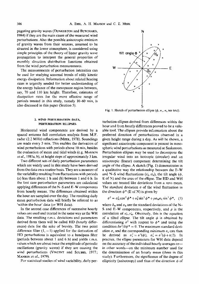
5 Fig. 1. Sketch of perturbation ellipse (#, c,, rr, see text).

turbation ellipses derived from differences within the hour and from hourly differences proved to be a valu- able tool. The ellipses provide information about the preferred direction of pe~~bations observed in a given height range during a day. As will be shown, a significant anisotropic component is present in mesospheric wind perturbations as measured at Saskatoon. Perturbation ellipses may be used to decompose the irregular wind into an isotropic (circular) and an anisotropic (linear) component dete~ining the tilt angle of the ellipse. A sketch (Fig. 1) demonstrates in a qualitative way the relationship between the E-W and N-S wind fluctuations (vh, z&), the tilt angle (4, E of N) and the axes of the ellipse. The HD and WH values are treated like deviations from a zero mean. The standard deviation G of the wind fluctuation in the direction # * (E of N) is given by

cr2 = ~~cos2~*+a~sin2#*+pa,o,sin2d,*, (1)

where 6, and (TV are the standard deviations of the N- S and E-W components, respectively, and p is the correlation of vf, &. Obviously, this is the equation of a tilted eliipse. The tilt angle ip is obtained by differentiating 0’ with respect to (p* and using the condition 6cr*/6$* = 0. The maximum standard deviation cx and the corresponding minimum (T,, can then be derived as 0,” = a’(4), a: = cr’($+~/2). In practice, the ellipse parameters for WH data depend on the accuracy of the individual hourly averages or- in other words---on the minimum number used for the determination of an hourly mean (three in this study). Furthermore, the significance of the degree of ellipticity (anisotropy) and thus of the direction 4 of

Horizontal wind fluctuations 387

the perturbation ellipse is a function of the number of

data points available. The degree of anisotropy can

be expressed by the standard deviation ratio ox/on. This ratio has been used to derive significance estimates for the daily perturbation ellipses (EBEL et al., 1985). Assuming that the wind fluctuations are isotropic and normally distributed in the horizontal

plane, frequency distribution functions of a,/o,, can be derived for samples with a given number of random wind fluctuation points (I&, vk). In this study the ratio exceeded by 20% (80% confidence limit) of the test

distribution proved to be a convenient measure of the significance of ellipticity and was applied where appropriate. The 80% confidence limit can be expressed as ox/o.n z exp(2.5/n”.6), where n > 5 is the number of data points used.

Time series of daily perturbation data for the height range from 61 to 110 km in steps of about 3 km

are used. Observations made from January 1979 till December 1983 are mainly analyzed. For 1984 standard deviation estimates are also employed, whereas tilt angle estimates derived for this year have not been included. This was done to avoid possible bias of the direction statistics due to missing WH data for October/November 1984 caused by a failure of the data processing system. Figure 2 gives an impression of how the anisotropic component of daily perturbation ellipses from HD data at various height ranges may be distributed. Each circle represents one height interval of 3 km starting at 61 km height (‘point 1) and ending around 117 km height (point 20). Filled circles indicate that the axial ratio of the relevant ellipse is exceeding the 80% confidence limit. The anisotropic component is expressed as a vector from the origin of the uk/u& coordinate system to a given circle. Its length is defined by o. = (CT: - a,$ I/‘, whereas its direction corresponds to the tilt angle 4 (E of N). This angle is only determined mod (n) by definition. Therefore, each vector tip is plotted twice in Fig. 2, namely with the directions 4 and C$ + 180 degrees.

In spite of the scatter, which is typical of most days, the majority of data points in Fig. 2 can easily be combined in three groups containing the anisotropic components of several adjacent levels. The preferred direction is in the N-S sector which contains all vectors exceeding the 80% confidence limit for the standard deviation ratio o,/o~. As will be demonstrated below, the N-S sector is one of the preferred sectors of wind perturbation directions.

For the interpretation of the perturbation direction statistics described in the following section it is essen- tial to keep in mind that the perturbation ellipses are derived from daily WH and HD sets representing the daily mean behaviour of horizontal wind disturb-

DAY 362 , 1983

1 : 61 km X):88km

% N

Yh

Ah I 3 km

Fig. 2. Tilt angle and anisotropic component (r.m.s. amplitude, given by the distance from the origin of the coordinate system) of perturbation ellipses for day 362, 1983, derived from WH data. Horizontal projections for height ranges of 3 km starting with 61 km (point 1) height. Filled circles indicate ellipses with axial ratios exceeding the 80% con-

fidence limit.

antes. One way to generate anisotropy of the wind

perturbations is the appearance of a single wave at a certain time of the day, or of a sequence of single gravity waves, or of wave groups (WEINSTOCK, 1976, 1984) with preferred direction of horizontal propagation adding fluctuations to an otherwise isotropic perturbation field (e.g. isotropic 2-dimensional tur- bulence; GAGE, 1979). Another way is to assume an initially isotropic distribution of horizontal wind per-

turbations due to gravity waves. Any process leading to elimination of a fluctuation component, e.g. by directional filtering of vertically propagating waves, or causing a weakening, e.g. by breaking or dissipation, in a given direction will result in elliptical elongation of the perturbation distribution in the per- pendicular direction. Furthermore, anisotropy of the perturbation windfield can be generated by sources exhibiting anisotropic emission characteristics for the amplitudes and/or directions of vertically propagating gravity waves. Several cases giving evidence that the preferred direction of wind perturbations at higher levels was determined by anisotropic gravity wave emission at lower atmospheric levels have been analyzed by MAN~~N et al. (1979).

388 A. EBEL, A. H. MANSON and C. E. MEEK

3. PERTURBATION DIRECTIONS AND INTENSITIES

Perturbation direction distributions have been

derived for the HD and WH data by determining the

relative frequency (in per cent) of the occurrence of ellipse tilt angles for individual months in eighteen 10” intervals (starting with O-9.9” ; average value 5.6% per 10” interval). The application of relative frequencies of occurrence is a convenient way to eliminate the influence of the variable number of observations per month. This number is affected by various exper-

imental conditions, especially for partial reflection, which are out of the scope of this study. The relative

frequencies have been smoothed using a three point gliding average (1, 1, 1 filter) for the direction intervals. Direction distributions have been prepared for

the height ranges 61-73, 76-97 and 10&l 14 km and the total range from 61 to 114 km. Except for a 5 yr composite, only results derived for the total height

range are employed in this study in order to achieve better statistical significance of the distribution functions. Daily data from 19 levels were used (maximum of 34,694 data points in 5 yr). For the HD component

72% of the maximum number of data was obtained without applying the 80% confidence limit. This limit

is not exceeded by 52% of the estimates. The respect-

ive values are 88% and 39% for the WH data (see Fig. 3). Monthly values of the maximum standard deviation cX have been used as a measure of the wind

perturbation intensities and its seasonal changes (Figs. 10 and 11).

The frequency of occurrence of perturbation directions for 1979-1983 is shown in Fig. 3. The direction distribution curve of the HD sample indicates that the

longer period fluctuations preferably occur in the E- W sector (around 90”) and in the N-S sector (around

O/180’). About two-thirds of the measured HD per-

turbation ellipses not exceeding the 80% confidence

limit for their axial ratios form a nearly isotropic

direction distribution (broken line in Fig. 3). This is also found for the WH data, where about half of the

measured perturbation ellipses do not exceed the 80%

confidence limit. This result indicates that the 80% confidence limit is an appropriate choice for the sep- aration of isotropic and anisotropic cases. The out-

standing feature of this data set is the pronounced maximum of the frequency of occurrence showing up around the N-S direction, with a slight bias towards the NE-SW sector, and a clear minimum around 135” (NW-SE sector). A secondary maximum is found in the E-W sector. It reflects properties of the HD distribution curve but may disappear or be flattened during individual years (e.g. 1982, 1983 in Fig. 6b).

Better insight into the significantly different prop-

0 90 180

s _ i._,_. 1809~.----_--..

.___.-- ( 52cyo) \.“,--_----*‘* 2 8@J $ m 2x0- WH

1600

1200

800

I c 0 90 INI

DIRECTION (degrees) Fig. 3. Histogram of perturbation ellipse tilt angles for 10” intervals, 1979-1983. Continuous line : without application of 80% confidence limit. Broken line: cases not exceeding the 80% confidence limit. Total number of angles and their fraction of maximum possible cases (in %) indicated at the curves. HD : period range t-6 h. WH : period range

I O-60 min.

erties of the statistics and climatology of the HD and WH wind perturbations is achieved when 5 yr averages of the monthly direction distribution functions are regarded. They are shown in Fig. 4a, b with and without application of the 80% confidence limit. By

eliminating the more isotropic background with axial ratios of perturbation ellipses below the 80% confidence limit the contours of the distribution plots become more pronounced. Otherwise the main structures of the contour plots for the HD and WH

data, respectively, are rather similar. The E-W maximum of the HD direction dis-

tribution in Fig. 3 appears to be a persistent feature over the year, with somewhat reduced values in May and September. The annual N-S maximum is mainly due to an increased number of fluctuations in this direction during the summer months, which are also mainly responsible for the appearance of a mean annual minimum in the NW-SE sector. The minimum around 45” appears to be mainly caused by the months around the equinoxes.

The seasonal change of the shorter period WH direction distributions (Fig. 4b) exhibits similar features to the HD distributions for January to April but with a stronger N-S maximum, a reduced minimum


HD 1979-1963. no conf. limit, 61-114 km

0 L5 90 us HI

DIRECTION ( degrees 1

HD 1979 -1963 , 80% conf. limit, 61-114 km

Ls 1;s l&l


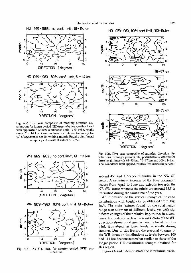
Fig. 4(a). Five year composite of monthly direction distributions for longer period (HD) perturbations, without and with application of 80% confidence limit. 197Sl983, height range 61-114 km. Contour lines for relative frequency (in %) of occurrence per 10” within a month. Equally distributed

samples yield constant values of 5.6%.

WH 1979-1963. no conf. limit, 61-114 km

0 L5 90 135 160


WH 1979 -1983, 80% conf. limit, 6l-114km

DIRECTION 1 degrees 1

Fig. 4(b). As Fig. 4(a), for shorter period (WH) perturbations.

HD 1979-1983. Kt%conf.limit. XX)-114km

3 3

f

1

6 6

9 9

12 2

75-97 km

0 L5 90 135 160

km

3 3

f

S6 6

E9 9

12 12

0 15 96 135 lffi

DIRECTION (degrees I

Fig. 5(a). Five year composite of monthly direction distributions for longer period (HD) perturbations, derived for three height intervals 61-73 km, 76-97 km and lOCL114 km. 80% confidence limit applied, relative frequencies in per cent.

around 45” and a deeper minimum in the NW-SE sector. A prominent increase of the N-S maximum

occurs from April to June and extends towards the NE-SW sector whereas the minimum around 135” is intensified during the same time of the year.

An impression of the vertical change of direction distributions with height can be obtained from Fig. 5a, b. The main features found for the total height range also show up at different levels, yet with significant changes of their relative importance in several cases. For instance, a clear E-W maximum of the WH directions shows up at greater heights for all months while it is absent at lower levels, especially during summer. Due to this feature the seasonal changes of the WH direction distributions at levels between 100 and 114 km become somewhat similar to those of the longer period HD distribution changes obtained for this region.

Figures 6 and 7 demonstrate the interannual varia-

390 A. EBEL, A. H. MAN~~N and C. E. MEEK

WH 1979 - 1983,60% conf. limit, ?00-1lC km

0 135 180

76-97km

3 3 rE S6 6

Y3 9

l2 12

0 135 180

61-73 km

3 3 r

6

9

12 12

0 L5 90 135 180

DIRECTION i degrees 1

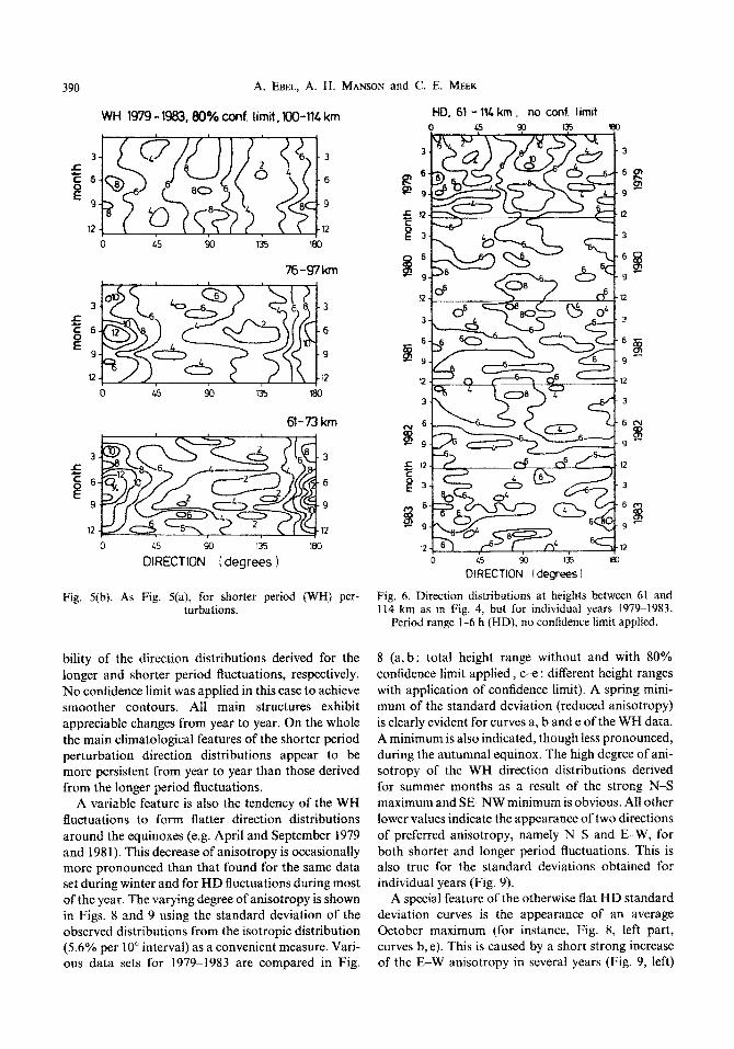
Fig. 5(b). As Fig. 5(a), for shorter period (WH) per- Fig. 6. Direction dist~b~tions at heights between 61 and turbations. 114 km as in Fig. 4, but for individual years 1979-1983.

bility of the direction distributions derived for the longer and shorter period fluctuations, respectively. No confidence limit was applied in this case to achieve smoother contours. A11 main structures exhibit appreciable changes from year to year. On the whole the main climatological features of the shorter period perturbation direction distributions appear to be more persistent from year to year than those derived from the longer period fluctuations.

A variable feature is also the tendency of the WH fluctuations to form flatter direction distributions around the equinoxes (e.g. April and September 1979 and 198 1). This decrease of anisotropy is occasionally more pronounced than that found for the same data set during winter and for HD fluctuations during most of the year. The varying degree of anisotropy is shown in Figs. 8 and 9 using the standard deviation of the observed distributions from the isotropic distribution (5.6% per 10” interval) as a convenient measure. Vari- ous data sets for 1979-1983 are compared in Fig.

HO, 6t - 1% km 1 no conf. limit 0 Is 135 180

b DIRECTION I degrees 1

Period range I-6 h (HD), no confidence limit applied.

8 (a, b: total height range without and with 80% confidence limit applied, c-e : different height ranges with application of confidence limit). A spring minimum of the standard deviation (reduced anisotropy) is clearly evident for curves a, b and e of the WH data. A minimum is also indicated, though less pronounced, during the autumnal equinox. The high degree of anisotropy of the WH direction distributions derived for summer months as a result of the strong N-S maximum and SE-NW minimum is obvious. All other lower values indicate the appearance of two directions of preferred anisotropy, namely N-S and E-W, for both shorter and longer period fluctuations. This is also true for the standard deviations obtained for individual years (Fig. 9).

A special feature of the otherwise flat HD standard deviation curves is the appearance of an average October maximum (for instance, Fig. 8, left part, curves b, e). This is caused by a short strong increase of the E-W anisotropy in several years (Fig. 9, left)


WH , 61 - 111 km, no conf. limit 0 65 90 135 lfn

0 L5 90 135 DIRECTION ( degrees)

180

Fig. 7. As Fig. 6, period range l&60 min (WH).

and at various levels. It is probably related to seasonal circulation changes as discussed below.

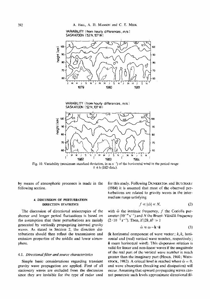
Both the HD and WH maximum r.m.s. deviations (0,) exhibit a dominant annual variation above, say, 95 km altitude, as demonstrated in Figs. 10 and 11, respectively. Between about 80 and 95 km a semiannual oscillation is clearly visible. It is more pronounced in the shorter period fluctuations and extends downward to lower levels in this case. For the longer period (HD) fluctuations it is found that the semiannual variation of the intensity is strongly reduced at heights below the mesopause. Clear seasonal

changes of perturbation kinetic energy as a function of height have been found to exist, e.g. by MANSON et al. (1975), and can also be inferred from the contour lines in Figs. 10 and 11. The magnitude of the respective energy density scale heights is about 68 km at altitudes around 90 km (MEEK et al., 1985b).

As regards possible causes of the measured wind fluctuations analyzed in this section, it cannot be

HD. 1979-1963 WH. 1979-1983 ,“““““‘+,~ 3tLLyLLLLLu-t

- lb I I / \ bl -

0 ,,,- ,(,, ((,, 10 JMHJSN JMM,SN

month month

Fig. 8. Standard deviations from isotropic distribution derived from the relative frequencies of occurrence (in X) of the 18 perturbation directions for the period 1979-1983 (Figs. 4 and 5) as a function of month. Left part: from longer period (HD) fluctuations; right part : from shorter period (WH) fluctuations. (a) 61-l 14 km, without confidence limit; (b)-(e) with 80% confidence limit for the total height range (b), lot&l14 km (c), 76100 km (d), 61-73 km (e). Note

different vertical scales for various parts of the figure.

HD. 61 -1lL km WH, 61 - 11L km

JMMJSN

month

1979

1980

1981

1982

1983

month Fig. 9. As Fig. 8 for individual years, 61-l 14 km altitude, no

confidence limit applied.

excluded that experimentally induced scatter con- tributes to the HD and WH perturbations. Yet it is certainly difficult to explain the seasonal, interannual and vertical changes of the perturbation anisotropy and r.m.s. deviation and the pronounced differences between the shorter and longer period fluctuations by experimental scatter. A posteriori we conclude that the experimental scatter is of preferably isotropic nature. An attempt to explain the main anisotropic features of the perturbation direction distributions

392 A. EBEL, A. H. MANSON and C. E. bfEEK

VARIABILITY 1 from hourly differences, m/s ) SASKATOON i 52 N ,107 W I

Fig. 10. Variability

J M M J 5 N’J M M J S N’J M M J 5 N’

5979 1980 1981

z i .P 2

VARIABILITY I from hourly differences, m/s ) SASKATOON I 52 N ,107 W 1

JMNJSNJMMJ

1982 ’ SNIMMJSN

1983 1984 (maximum standard deviation, in m s- ‘) of the horizontal wind in the period range

I-6 h IHD data).

by means of atmospheric processes is made in the following section.

4. ~ISC~~~ON OF PERTURBATION DIRECTION STATISTICS

The discussion of directional anisotropies of the shorter and longer period fluctuations is based on the assumption that these perturbations are mainly generated by vertically propagating internal gravity waves. As stated in Section 2, the direction distributions should then reflect the transmission and emission properties of the middle and lower atmosphere.

4.1. Dir~c?i@na~~lt~~ and source &hara~t~ri~tics

SimpIe basic considerations regarding transient gravity wave propagation are applied. First of all stationary waves are excluded from the discussion since they are invisible for the type of radar used

for this study. Following DUNKBRTON and BUTCHART (1984) it is assumed that most of the observed perturbations are related to gravity waves in the inter- mediate range satisfying

f << Id31 << fV, (2)

with &r the intrinsic frequency, f the Coriolis par- ameter (1 0w4 s - ‘) and N the Brunt-VaisHli frequency (2. IO-’ s-l). Then, if 12k,HI >> 1

& z co-k-ii (31

(k horizontal component of wave vector; ic, k, hori- zonta1 and (real) vertical wave number, respectively ; I mean horizontal wind). This dispersion relation is valid for linear and non-linear waves if the magnitude of the real part of the vertical wave number is much greater than the imaginary part (HINES, 1960 ; WEIN- STOCK, 1982). A critical level is reached where & = 0, and wave absorption (breaking and dissipation) will occur. Assuming that upward propagating waves cannot penetrate such levels approximate directional fil-

Horizontal wind fluctuations

VARIABILITY I WH, m/s 1 SASKATOON ( 52 N. 107 W 1

393

VARIABILITY ( WH, m/s 1 SASKATOON I 52 N .x)7 W 1

I ,

JMMJSNJ MMJSNJMMJSN

1982 1983 198L

Fig. Il. As Fig. 10 for the period range IO-60 min (WH data).

ters can be derived from equation (3) and designed for a given wave- and windfield from the critical level

condition

c = cos au, (4)

where c = o/k > 0 is the horizontal phase speed of the wave propagating in the direction of k, cos a = (k - ii)/kti with a the angle between the mean flow and horizontal wave vector, and U = 1111. Break- ing, which can occur for waves with small deviations from the critical level condition, will be neglected in

the following considerations since this effect would only slightly change the gross filter characteristics derived below with simplifying assumptions.

Let us consider a flow which is eastward at all

altitudes below the height range of observation but with a height dependent speed ranging between zero and a maximum value uO. Then all phase velocities which are forbidden according to equation (4) lie within a circle with a radius of uo/2 with its center at (24,,/2,0) when plotted in a phase velocity diagram with eastward velocities in the positive x-direction and northward components in the positive y-direction. Exam-

ples of this case may be found in Fig. 13 (areas within the large circles of cases A and B). Evidently, the most favourable sector for perturbation directions would

be orthogonal to the mean flow direction if one takes into account that the perturbation directions can only be determined mod (7~). This result for transient waves with c # 0 is quite different from what is found for the special case of stationary waves, which are mainly prohibited in the direction orthogonal to the mean flow and travel preferably in or against the wind direction (DUNKERTON and BUTCHART, 1984). It can there-

fore be expected that momentum deposition, generation of eddy diffusivity and related effects are different for both types of anisotropic (filtered) wave ensembles.

The horizontal wind vector ii varies on short time scales, for instance due to planetary wave activity, and may introduce stochastic changes in the transmission condition as derived from equations (3) and (4). Yet to avoid unnecessary complications we will focus on mean vertical windfields derived for larger areas and longer time periods of, say, one month or more in the following discussion. Examples of zonal mean wind


1 ‘1’ ’ i ’ ’ ‘4 t

-Eel -40 -a, 0 20 u3 w @I

mean zonal wind [ m/s 1

Fig. 12. Vertical profiles of mean zonal winds. Continuous curves (CIRA 72) : zonal averages after KANTOR and COLE (1964) for 50”N. Broken curves (MM84) : time and regional

averages after MEEK and MAN~ON (1985).

profiles for the latitude of Saskatoon are contained in

Fig. 12. Guided by these profiles we have composed a few filter characteristics for ‘winter’ and ‘summer’ conditions by means of equation (4). They are reproduced in Fig. 13, where hatched areas indicate velocities of waves unable to penetrate to greater heights. Example A is based on the assumption that the flow is eastward ($,, = 90°) at all heights : u, < u ,< u. corresponds to the January profile MM84 in Fig. 12

(u, = 20 m/s, u0 = 50 m/s). For cases B-D it has been assumed that two wind regimes exist with different

mean directions and maximum speeds 40, u0 and 4 ,, u,, respectively, and that the speed varies between zero and its maximum value in both regimes. In this

way we can separate the windfield into a stratospheric/lower mesospheric (index 0) and a tropospheric (index 1) regime. This is especially advan- tageous for ‘summer’ conditions (cases CD) with westward flow (4,, = -90°) above and eastward wind components below the tropopause. A direction of 4, = 120 and 150” has been adopted for cases C and D, respectively. Case B represents directional filtering by a stronger westerly flow at upper layers and weaker northwesterlies in the troposphere. The parameters used for all filters are compiled in Table 1. A range

c d c0 with c,, close to zero (stationary waves) is excluded due to reasons already mentioned. Obviously, directional filters also taking into account meridional wind components at higher levels can be designed simply by rotating the respective zonal filter characteristic somewhat towards north or south. Examples of filters derived from more complex windfields generated by a 3-D circulation model are shown by JAKOBS et al. (1986).

If the phase velocity spectrum of gravity waves

entering the prescribed windfield is known, direction

distributions can be derived for the height range above

a given level (lowest altitude of measurements).

Nothing precise is known about the gravity wave spec-

trum in the source region (tropospheric layers). There- fore, as a first guess, an isotropic Gaussian distribution has been adopted for gravity waves with

phase speeds c

G(c) N exp (- c’/2af)

(0, the r.m.s. deviation of c). This function can be weighted with respect to direction 4 by a function S(4), thus simulating certain possible source characteristics like more intense gravity wave emission in

the E-W-direction or arrival of more waves from the

southern sector. S(4) = 1 +cos4(4 -90’) has been used for the former and S(4) = 1+0.3 cos 4 with 14 1 < 90” for the latter case (Table 1, Fig. 15). The

frequency of occurrence of perturbation directions with a given angle 4 is then obtained (in arbitrary units) by integrating over the part of the distribution

functions S(4) * G(c) and S(4 + 180”) * G(c) where vertical wave propagation is allowed according to the adopted transmission function and by adding the result for both directions. [Note again that the perturbation direction is only given mod(w).] Two examples are shown in Fig. 14, namely for the

directional filter A in Fig. 13 along the E-W-axis (4 = 90”) and the filter D along the broken line. Forbidden phase velocities are indicated by hatching.

S(4) = 1 and gr = 30 m s-’ have been chosen. The latter value has been adopted in order to have G(c)/G(O) = l/e at a phase speed near 40 m s- ‘.

Several examples of distribution functions mod-

elled in the outlined way are exhibited in Fig. 15. The corresponding parameters are also found in Table 1. For convenience, several parameters have been kept constant for all cases : oc = 30 m s- ’ (standard deviation of c), u0 = 50 m s-’ (maximum of the strong

wind regime), u, = 25 m se ’ (maximum for weak wind regime ; not needed for filter A, including distribution 1 b where westerlies between 20 and 50 m s- ’ have been adopted). The quasi-stationary fraction is determined from the assumption that it contains 20% of the waves for a given direction of horizontal propagation.

From the adopted numbers it follows that waves with phase speeds c d c0 = 7.5 m so ’ are eliminated from the spectrum.

4.2. Modelled and observed direction distributions

As a general result we note the appearance of frequency maxima in the N-S sector (O/180”) for all


winter summer

s s Fig. 13. Directional filtering due to the critical level condition for transient internal gravity waves with phase speed c # 0 in a phase velocity coordinate system. Two wind regimes in the vertical with different mean maximum speeds and directions assumed for cases ED. Westerly wind band for example A. Vectors C represent arbitrary phase velocities. For broken line refer to Fig. 14. For more details see text and

Table 1.

Table 1. Parameters of direction distribution models (Figs. 13 and 15)

No. of curve Sketch, % in Fig. 15 Fig. 13 (m SK’)

la lb 2 3 4 5

6 7

Directional filter Weighting function S(4)

- 50 50 50 50 50 50

D 50 270 25 150 C 50 270 25 120

dh

90 90 90 90

270 270

UI (m s-‘) +I

0 20* 90

0 25 120 25 120 25 120

UC (m s- ‘)

30 30 30 30 30 30

30 30

Direction of maximum weight S(4)

- 1 I

E, W 1+ cos4 (4 - 90)

E, W 1+ co? (4 - 90) 1

N lif90<4<270, 1+0.3.cos~, if-90<+<90 1

E, W 1+ cos4 (f#J - 90)

uO, a, : maximum speed of two mean wind regimes. +0, 4, : direction of mean wind with N = o”, E = 90”, etc. (r, : r.m.s. deviation of normal phase speed distribution. 4 : direction of phase velocity in degrees. * Curve 1 b : u, is the minimum speed of the adopted west wind band (see text).

modelled distributions due to the dominance of strong Fig. 15, curves 4 and 6 for isotropic sources). Yet westerlies or easterlies in general accordance with the several features emanate from the direction statistics observations (e.g. Fig. 4). Furthermore, it is relatively where the explanation in terms of transmission prop- easy to generate asymmetries about the N-S direction erties only is less straightforward or impossible. which are mainly found for shorter (WH) and longer Such features are : the appearance of a strong E-W period (HD) fluctuations during summer, by intro- anisotropy of the perturbation directions, mainly for ducing mean summer meridional winds in the lower longer period (HD) fluctuations, but also for shorter and/or upper filtering layers of the atmosphere (see period disturbances in winter; the tendency of this

396 A. EBEL, A. H. MANKIN and C. E. MEEK

-2 i c/d

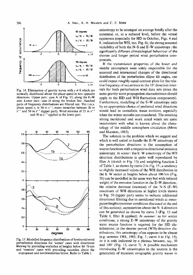
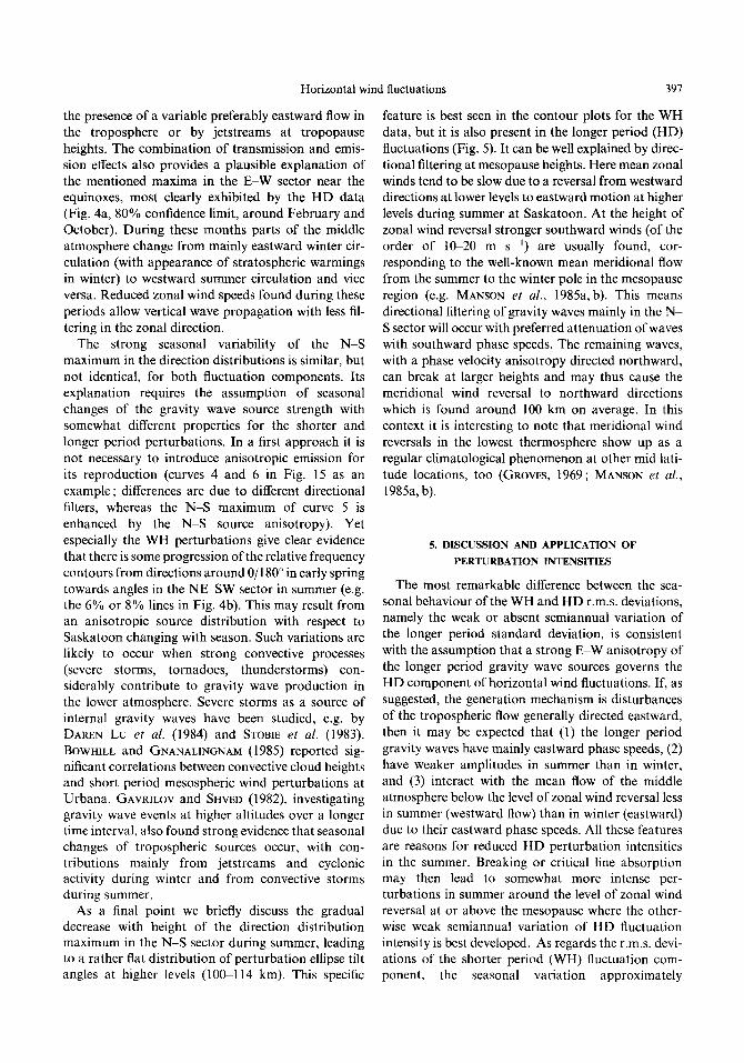
Fig. 14. Elimination of gravity waves with c # 0 which are normally distributed about the phase speed in two opposite directions. Upper part: case A of Fig. 13, along the E-W axis. Lower part: case D along the broken line. Hatched parts of frequency distributions are filtered out. The r.m.s. phase speed (TV is 30 m K’, mean westerlies between 20 m SK’ and 50 m s- ’ (upper part). Wind maxima of 25 m s- ’

and 50 m s- ’ applied in the lower part

,OO

I ’ ’ ’ ’ *

0.6 - I’

0.6 -

O.1 I_ 0 J) 60 w 120 150

degrees

Fig. 15. Modelled frequency distributions of horizontal wind perturbation directions for ‘winter’ cases with directional filtering by prevailing westerlies at heights below 6(t70 km and ‘summer’ cases with prevailing easterlies above the

tropopause and northwesterlies below. Refer to Table 1.

anisotropy to be strongest on average briefly after the autumnal or, at a reduced level, before the vernal equinoxes (especially for HD in October, Figs. 4 and 8 ; indication for WH, too, Fig. 4) ; the strong seasonal variability of both the N-S and E-W anisotropy ; the significantly different climatological behaviour of the shorter and longer period wind perturbation components.

If the transmission properties of the lower and middle atmosphere were solely responsible for the seasonal and interannual changes of the directional distribution of the perturbation ellipse tilt angles, one could expect roughly equal contour plots for the relative frequency of occurrence in the 10” direction intervals for both perturbation wind data sets (since the same gravity wave propagation characteristics should apply to the HD and WH fluctuation components). Furthermore, modelling of the E-W anisotropy only by an appropriate choice of preferred wind directions would lead to unrealistic mean motions, especially when the winter months are considered. The resulting strong meridional and weak zonal winds are quite inconsistent with what is known about the climatology of the middle atmosphere circulation (MEEK

and MANSON, 1985). The solution to the problem which we suggest and

which is well suited to handle the E-W anisotropy of

the perturbation directions is the assumption of source functions with a respective directional emission

anisotropy. In winter : the E-W anisotropy of the HD direction distributions is quite well reproduced by filter A (sketch in Fig. 13) and weighting function 2

of Table 1, as shown by curve 2 in Fig. 15 ; a tendency to slightly increased values of the WH distribution in the E-W sector at heights below about 100 km (Fig. 5b) can be modelled in the same way but with reduced weight of the emission function in the E-W direction ; the relative decrease (increase) of the N-S (E-W) maximum of WH directions at higher levels shown in Fig. 5b (upper part) seems to indicate additional directional filtering due to meridional winds at mesopause heights (summer conditions discussed at the end of this section) ; asymmetries about the N-S direction can be generated as shown by curve 3 (Fig. 15 and Table 1, filter B applied). In summer : as for winter conditions, a strong E-W anisotropy of the gravity wave source function is required for the HD distributions; in the shorter period (WH) direction distributions, this anisotropy often appears to be absent (e.g. summer 1981, 1983, Fig. 7 ; curve 4 in Fig. 15), or it is only indicated by a plateau between, say, 50 and 100” (Fig. 15, curve 7). A possible mechanism introducing E-W anisotropies in the sources is the generation of transient orographic gravity waves in


the presence of a variable preferably eastward flow in the troposphere or by jetstreams at tropopause heights. The combination of transmission and emission effects also provides a plausible explanation of the mentioned maxima in the E-W sector near the equinoxes, most clearly exhibited by the HD data

(Fig. 4a, 80% confidence limit, around February and October). During these months parts of the middle atmosphere change from mainly eastward winter circulation (with appearance of stratospheric warmings in winter) to westward summer circulation and vice versa. Reduced zonal wind speeds found during these

periods allow vertical wave propagation with less filtering in the zonal direction.

The strong seasonal variability of the N-S maximum in the direction distributions is similar, but not identical, for both fluctuation components. Its explanation requires the assumption of seasonal changes of the gravity wave source strength with somewhat different properties for the shorter and longer period perturbations. In a first approach it is not necessary to introduce anisotropic emission for its reproduction (curves 4 and 6 in Fig. 15 as an

example ; differences are due to different directional filters, whereas the N-S maximum of curve 5 is

enhanced by the N-S source anisotropy). Yet especially the WH perturbations give clear evidence that there is some progression of the relative frequency contours from directions around O/l 80” in early spring towards angles in the NE-SW sector in summer (e.g. the 6% or 8% lines in Fig. 4b). This may result from an anisotropic source distribution with respect to Saskatoon changing with season. Such variations are likely to occur when strong convective processes (severe storms, tornadoes, thunderstorms) con- siderably contribute to gravity wave production in the lower atmosphere. Severe storms as a source of internal gravity waves have been studied, e.g. by DAREN Lu et al. (1984) and STOBIE et al. (1983). BOWHILL and GNANALINGNAM (1985) reported significant correlations between convective cloud heights and short period mesospheric wind perturbations at Urbana. GAVRILOV and SHVED (1982), investigating gravity wave events at higher altitudes over a longer time interval, also found strong evidence that seasonal changes of tropospheric sources occur, with con- tributions mainly from jetstreams and cyclonic activity during winter and from convective storms during summer.

As a final point we briefly discuss the gradual decrease with height of the direction distribution maximum in the N-S sector during summer, leading to a rather flat distribution of perturbation ellipse tilt angles at higher levels (100-l 14 km). This specific

feature is best seen in the contour plots for the WH

data, but it is also present in the longer period (HD) fluctuations (Fig. 5). It can be well explained by directional filtering at mesopause heights. Here mean zonal winds tend to be slow due to a reversal from westward directions at lower levels to eastward motion at higher levels during summer at Saskatoon. At the height of zonal wind reversal stronger southward winds (of the order of 10-20 m s- ‘) are usually found, corresponding to the well-known mean meridional flow from the summer to the winter pole in the mesopause

region (e.g. MANSON et al., 1985a, b). This means directional filtering of gravity waves mainly in the N- S sector will occur with preferred attenuation of waves with southward phase speeds. The remaining waves, with a phase velocity anisotropy directed northward, can break at larger heights and may thus cause the meridional wind reversal to northward directions which is found around 100 km on average. In this context it is interesting to note that meridional wind reversals in the lowest thermosphere show up as a regular climatological phenomenon at other mid latitude locations, too (GROVES, 1969; MANSON et al., 1985a, b).

5. DISCUSSION AND APPLICATION OF

PERTURBATION INTENSITIES

The most remarkable difference between the seasonal behaviour of the WH and HD r.m.s. deviations, namely the weak or absent semiannual variation of the longer period standard deviation, is consistent with the assumption that a strong E-W anisotropy of the longer period gravity wave sources governs the HD component of horizontal wind fluctuations. If, as suggested, the generation mechanism is disturbances

of the tropospheric flow generally directed eastward, then it may be expected that (1) the longer period gravity waves have mainly eastward phase speeds, (2) have weaker amplitudes in summer than in winter, and (3) interact with the mean flow of the middle atmosphere below the level of zonal wind reversal less in summer (westward flow) than in winter (eastward) due to their eastward phase speeds. All these features

are reasons for reduced HD perturbation intensities in the summer. Breaking or critical line absorption may then lead to somewhat more intense perturbations in summer around the level of zonal wind reversal at or above the mesopause where the otherwise weak semiannual variation of HD fluctuation intensity is best developed. As regards the r.m.s. deviations of the shorter period (WH) fluctuation component, the seasonal variation approximately


resembles that simulated by GARCIA and SOLOMON (1985) using a 2-dimensional dynamical model.

The climatology of the maximum r.m.s. deviation flX is of special importance for applications in numerical modelling of the middle atmosphere. The vertical eddy diffusivity D, is roughly proportional to o: (WEINSTOCK, 1984). D,, w ycrz, with y = I s, seems to be a reasonable estimate for Saskatoon. It is emphasized that a: derived from the WH data is consider- ably larger than values based on HD fluctuations, especially when a decrease of the r.m.s. deviations by a factor of approximately 0.5 is taken into account to reduce CT,, derived for HD, to gravity wave amplitudes (VINCENT and STUBBS, 1977). The vertical eddy diffusivity should therefore mainly be determined by the shorter period ~rturbations. Measurements of gravity wave momentum deposition (VINCENT and REID, 1983 ; REID, 1984; REID and VINCENT, 1987) also show that the shorter period range is the more efficient one.

Another quantity urgently needed for numerical simulation of the upper middle atmosphere is the dissipation rate of eddy kinetic energy since it may con- stitute a significant, if not dominant, term of the energy balance at lower thermospheric heights. GARTNER and MEM~~I~R (1984), using a 2- dimensional numerical model of the middle atmosphere, demonstrated that then appreciable changes of the mean meridional flow at these altitudes may occur when compared to simulation experiments without inclusion of perturbation kinetic energy dissipation. It is therefore appropriate to include a short discussion of eddy kinetic energy dissipation rates E which can be estimated from monthly (climatological) values of short period wind fluctuations. Only r.m.s. deviations of the larger perturbations in the period range from 10 to 60 min will be applied.

A widely used relation between E and vertical eddy diffusivity is F = N2D, (e.g. EBEL, 1984). Scaling Dzz as before and using N = 2 = IO-’ s- ‘, one has ~=0.08Wkg~~for~,~=200m2s~2atabout90km altitude. An alternative way to estimate perturbation kinetic energy dissipation is possible. It shows the uncertainties involved in the determination of E. On the other hand, it also provides values fitting into the range of recently published estimates (e.g. HOCKING, 1985) and is therefore briefly described here. The dissipation rate E of gravity wave kinetic energy can be approximated as follows

E z D,,((&d/~z)‘+(W/~z)‘)

w D,(~~(u’~+ P))

= D;jc~2(~‘2+d2). (5)

The angle brackets denote ensemble or space/time averaging (WEINSTOCK, 19761982) and k,* is a typical wave num~r for dissipation processes. z, u’ and u’ are, respectively, height and zonal and meridional wind perturbation due to gravity waves. We try to relate expression (5) to the observed r.m.s. amplitudes of the WH fluctuations in the 10-60 min period range. Assuming (~‘~fv’~) x 02 and D, z yoz as before one has

F = Bis,4. (6)

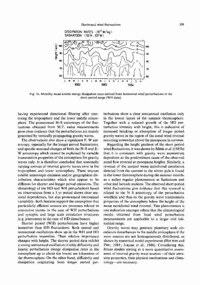
B = yk,*’ may be a complex function of height, geo- graphic coordinates and season. Evidently, B is difftcult to determine without more thorough information about the gravity wave field than is available in this case. As a first approximation, B is therefore kept constant with height and E is again scaled with a plausible value near 90 km height. Assuming that both approximations for E agree around this height (i.e. yN%: = Ba.: = 0.08 W kg-‘, N2 = 4. 1O-4 s-‘) B = 2 - 10m6 rn-’ s.“ is obtained. Using this value and equation (6), climatological estimates of E can easily be derived from the 6, contours in Fig. 11 (WH data). For the purpose of discussion a part of the estimates is reproduced in Fig. 16.

It is obvious that a relatively strong increase of E with height occurs due to the dependence of the estimates in Fig. 16 on a;‘. The more frequently used estimate N’D, yieids values less (larger) by a factor of 5 at the highest (lowest) levels analyzed in this study. Radar measurements (HOCKING, 1983) seem to indicate that equation (6) underestimates E at lower levels. On the other hand, the values shown in Fig. 16 seem to fit estimates derived from rocket measurements by THRANE et cd. (1985) rather satisfactorily at lower heights. Values of E increasing with height between about 90 and 105 km at a similar large rate as in Fig. 16 have been reported by ROPER (1966). Estimates of E based on climatologi~l data of the mesopause region also tend to larger values (EBEL et a!., 1983). Despite the apparent uncertainties involved in the derivation of dissipation rates from short- period wind perturbations they clearly show the importance of heating due to eddy dissipation for the energy balance of the lower thermosphere and upper mesosphere (HINGS, 1965; GAVRILOV and SHVED, 1975 ; SCHOEBERL et al., 1983 ; EBEL, 1984).

6. CONCLUSION

Shorter (WH) and longer (HD) period wind fluctuations in the mesosphere and lower thermosphere at Saskatoon (52’N, 107”W) show properties that are characteristic of a transient internal gravity wave field

Horizontal wind fluctuations

DISSIPATION RATES ( 1O-2 W/kg ) SASKATOON ( 52 N ,107 W )

399

I ,““.‘,““I”““““,,’ JMMJSNJMMJSNJMMJSN

1982 1983 198.L

Fig. 16. Monthly mean kinetic energy dissipation rates derived from horizontal wind perturbations in the short period range (WH data).

having experienced directional filtering after trav- ersing the troposphere and the lower middle atmos-

phere. The pronounced N-S anisotropy of the fluctuations obtained from M.F. radar measurements gives clear evidence that the perturbations are mainly generated by vertically propagating gravity waves.

The observations also show a significant E-W anisotropy, especially for the longer period fluctuations, and specific seasonal changes of both the N-S and EP

W anisotropy which cannot be explained by variable transmission properties of the atmosphere for gravity waves only. It is therefore concluded that seasonally varying sources of internal gravity waves exist in the troposphere and lower stratosphere. These sources exhibit anisotropic emission and/or geographical distribution characteristics which also appear to be

different for shorter and longer period emissions. The climatology of the HD and WH perturbations based on observations from a 5 yr period shows clear seasonal dependences, but also pronounced interannual variability. Both features support the assumption that particularly efficient sources are processes related to convective storms in the case of WH perturbations

and synoptic and large scale circulation structures (e.g. jetstreams) in the case of HD disturbances.

Shorter period (WH) perturbations have higher intensities than HD fluctuations. Both annual and semiannual oscillations show up in the WH and HD perturbation intensities. Their relative importance changes with height. The shorter period data exhibit a strong semiannual oscillation of eddy diffusivity and kinetic perturbation energy dissipation rates in the mesosphere up to about the lowest ten kilometres of the thermosphere. On the other hand, diffusivity and dissipation originating from longer period per-

turbations show a clear semiannual oscillation only in the lowest layers of the summer thermosphere. Together with a reduced growth of the HD perturbation intensity with height, this is indicative of

increased breaking or absorption of longer period gravity waves in the region of the zonal wind reversal occurring somewhat above the mesopause in summer.

Regarding the height gradient of the short period wind fluctuations, it was shown by MEEK et al. (1985b)

that it is consistent with gravity wave momentum

deposition as the predominant cause of the observed zonal flow reversal at mesopause heights. Similarly, a

reversal of the normal mean meridional circulation directed from the summer to the winter pole is found in the lower thermosphere during the summer months

as a rather regular phenomenon at Saskatoon and other mid latitude stations. The observed short period wind fluctuations give evidence that this reversal is related to the N-S anisotropy of the perturbation windfield and thus to the gravity wave transmission properties of the atmosphere below the height of the mean meridional wind reversal. This phenomenon is

one indication amongst others that the climatological results obtained from local wind perturbation measurements are applicable to a larger mid lati- tudinal range.

Gravity waves may generate planetary scale cir-

culation disturbances in the middle atmosphere if the wave sources are not homogeneously distributed, as shown by numerical model experiments (HOLTON and ZHU, 1984; JAKOBS et al., 1986). Considering this, future studies aiming at a more quantitative assess- ment of internal gravity wave sources-of their emission properties, their physical mechanisms and climatology-are necessary.


Acknowledgements-Helpful and stimulating discussions Canada, by the Institute of Space and Atmospheric Studies, with I. M. REID are gratefully acknowledged. This work was University of Saskatchewan, Saskatoon, and by the sponsored by the Natural Sciences and Engineering Research Deutsche Forschungsgemeinschaft, F.R.G. (grants Eb Council and the Atmospheric Environment Service, both of 56/6-4,5 and Eb 56/10-l).

DAREN Lu, VAN ZANDT T. E. and CLARK W. L. DUNKERTON T. .I. and BUTCHART N. EBEL A. EBEL A., JAKOBS H. J. and SPETH P. FRITTS D. C. GAGE K. S. GARCIA R. R. and SOLOMON S. GARTNER V. and MEMMESHEIMER M. GAVRILOV N. M. and SHRED G. M. GAVRILOV N. M. and SHVED G. M. GROW G. V. HINES C. 0. HINES C. 0. HIROTA I. HOCKING W. K. HOCKING W. K. HOLTON J. R. HOLTON J. R. and ZHU X. JAKOBS H. J., BISCHOF M., EBEL A.

and SPETH P. KANTOR A. J. and COLE A. E. LINDZEN R. S. MANSON A. H., GREC~RY J. B. and

STEPHENSON D. G. MANSON A. H., MEEK C. E. and STENING R. J. MANSON A. H. and MEEK C. E. MANSON A. H., MEEK C. E. and GREGORY J. B. MANSON A. H., GREGORY J. B. and MEEK C. E. MANSON A. H., MEEK C. E., MASSEBEUF M.,

FELLOUS J. L., ELFORD W. G., VINCENT R. A., CRAIG R. L., ROPER R. G., AVERY S., BALSLEY B. B., FRASER G. J., SMITY M. J., CLARK R. R., KATO S., TSUDA T. and EBEL A.

MATSUNO T. MEEK C. E. and MANSON A. H. MEEK C. E., REID I. M. and MANSON A. H. MEEK C. E., REID I. M. and MANSON A. H. REID I. M. and VINCENT R. A. ROPER R. G. SCHOEBERL M. R., STROBEL D. F. and

APRUZESE J. P. STOBIE J. G., EINAUDI F. and UCCELLINI L. W. THRANE E. V., ANDREASSEN O., BLIX T.,

GRANDAL B., BREKKE A., PHILBRICK C. R., SCHMIDLIN F. J., WIDUEL H. U., VON ZAHN U. and L~~BKEN F. J.

VINCENT R. A. VINCENT R. A. and FRITTS D. C. VINCENT R. A. and REID I. M. VINCENT R. A. and STUBBS T. J. WEINSTOCK J. WEINST~CK J. WEINSTOCK J.

REFERENCES

1984 J. atmos. Sci. 41, 272. 1984 J. atmos. Sci. 41, 1443. 1984 J. atmos. terr. Phys. 46, 727. 1983 Annls Geophysicae I, 359. 1984 Rev. Geophys. Space Phys. 22,275 1979 J. atmos. Sci. 36, 1950. 1985 J. geophys. Res. 90,385O. 1984 J. atmos. terr. Phys. 46,755. 1975 Annls Geophys. 31, 375. 1982 Annls Geophys. 38,789. 1969 J. Br. interplanet. Sot. 22, 285. 1960 Can. J. Phys. 38, 1441. 1965 J. geophys. Res. 70, 177. 1984 J. atmos. terr. Phys. 46, 767. 1983 J. atmos. terr. Phys. 45, 103. 1985 MAP Handbook 16.290. 1982 J. atmos. Sci. 39, 791. 1984 J. atmos. Sci. 38, 2172. 1986 J. atmos. terr. Phys. 48, 1203

1964 J. geophys. Res. 69, 5 13 1. 1981 J. geophys. Res. 86,9707. 1975 J. atmos. Sci. 32, 1682.

1979 1980 1981a 198lb 1985a

J. atmos. terr. Phys. 41, 325. J. atmos. terr. Phys. 42, 103. J. geophys. Res. 86,96 15. Planet. Space Sci. 29, 615. Adv. Space Res. 5, 135.

1982 J. met. Sot. Japan 60, 215. 1985 J. atmos. terr. Phys. 47, 477. 1985a Radio Sci. 20, 1363. 1985b Radio Sci. 20, 1383. 1987 J. atmos. terr. Phys. (submitted for publication). 1966 J. geophys. Res. 71,4427. 1983 J. geophys. Rex 88,5249.

1983 J. atmos. Sci. 40, 2804. 1985 J. atmos. terr. Phys. 47,243.

1984 J. atmos. terr. Phys. 46, 119. 1987 J. atmos. Sci. (submitted for publication). 1983 J. atmos. Sci. 40, 132 1. 1977 Planet. Space Sci. 25,441. 1976 J. geophys. Res. 81,633. 1982 J. atmos. Sci. 39, 1698. 1984 J. atmos. terr. Phys. 46, 1069.

Reference is also made to the following unpublished material:

BOWHILL S. A. and GNANALINGNAM S. 1985 Workshop on Technical and Scientific Aspects of MST Radar, Puerto Rico, 3.24.

EBEL A., MANSON A. H. and MEEK C. E

MANSON A. H., MEEK C. E., MASSEBEUF M., FELLOUS J. L., ELFORD W. G., VINCENT R. A., CRAIG R. L., ROPER R. G., AVERY S., BALSLEY B. B., FRASER G. J., SMITH M. J., CLARK R. R., KATO S., TSUDA T. and EBEL A.

MEEK C. E.


REID 1. M.

1985

1985b

Report No. 5, Atmospheric Dynamics Group, Insti- tute of Space and Atmospheric Studies, University of Saskatchewan, Canada S7N OWO.

Report No. 4, Atmospheric Dynamics Group, Insti- tute of Space and Atmospheric Studies, University of Saskatchewan, Saskatoon, Canada S7N OWO.

1978 Report 2/78, Atmospheric Dynamics Group, Tnsti- tute of Space and ktmosph&ic Studies, University of Saskatchewan, Saskatoon. Canada S7N OWO.

1984 Ph.D. Thesis, University of Adelaide, Australia.

short period fluctuations of the horizontal wind measured in the upper middle atmosphere and...

Documents