setting setting biodiversity biodiversity prioritiespriorities · · 2013-06-20setting setting...

SETTING SETTING SETTING SETTING BIODIVERSITY BIODIVERSITY BIODIVERSITY BIODIVERSITY

PRIORITIESPRIORITIESPRIORITIESPRIORITIES

A paper prepared as part of the activities of the working group producing the report Sustaining our Natural Systems and

Biodiversity for the Prime Minister’s Science, Engineering and Innovation Council in 2002.

Hugh Possingham1, Sarah Ryan2, Jenny Baxter2 and Steve Morton2

1 The Ecology Centre, Department of Zoology and Department of Mathematics, University of Queensland

2 CSIRO Sustainable Ecosystems, Canberra

The authors are aware of the limitations of some of the assumptions and analyses in this paper. We encourage others

to debate the methodology and refine the data.

Many others contributed their expertise to the ideas in the paper and they are listed overleaf.

Setting Biodiversity Priorities

Background paper for PMSEIC report “Sustaining our Natural Resources and Biodiversity” 2 May 2002

Setting Biodiversity Priorities Workshop

A workshop to refine the approach in this paper and gather expert advice about biodiversity priorities was held 29-30 January 2002 in Bungendore. Participants were:

Jenny Baxter CSIRO Sustainable Ecosystems, Canberra Sue Briggs NSW NPWS, Canberra Mark Burgman Department of Botany, University of Melbourne Marc Carter Environmental Economics Unit, EA Paul Cristofani National Farmers' Federation Ltd Wendy Craik Earth Sanctuaries Limited Peter Cullen CRC for Freshwater Ecology, Canberra Jane Elix Community Solutions (facilitator) Michael Kennedy Humane Society International Max Kitchell Natural Heritage Division, Environment Australia Chris Margules CSIRO Sustainable Ecosystems, Atherton Paul Marsh Biodiversity Policy Section, Environment Australia Norm McKenzie CALM, WA Steve Morton CSIRO Sustainable Ecosystems, Canberra Henry Nix CRES, Australian National University Hugh Possingham Department of Zoology & Entomology, University of Queensland Rick Roush Weeds CRC, Adelaide Sarah Ryan CSIRO Sustainable Ecosystems, Canberra Paul Sattler NLWRA, Queensland Jann Williams Department of Geospatial Science, RMIT John Woinarski Parks and Wildlife Commission, NT

Paper available at http://www.dest.gov.au/science/pmseic/meetings/8thmeeting.htm.

http://www.dest.gov.au/science/pmseic/meetings/8thmeeting.htm



INTRODUCTION To arrive at our recommendations about priority actions for sustaining biodiversity and our natural resources, we have used a decision analysis approach. This is based on the general philosophy that underlies the Tela paper “The business of biodiversity” by Hugh Possingham, one of the working group members (Possingham 2001). Hugh argues that choosing between options to maximise long term biodiversity should be dealt with in a business-like way. While the currency of business is dollars and the currency of nature conservation is biodiversity, for a fixed financial investment we should aim to maximise our long-term biodiversity gains. Biodiversity gains overflow into other benefits for natural resources, and these are taken into account in the analysis.

The priority actions identified in National Objectives and Targets for Biodiversity Conservation 2001-2005 (Environment Australia 2001a), and referred to as NOTBC in this paper, were used as a starting point. These are:

1. Protect and restore native vegetation and terrestrial ecosystems

2. Protect and restore freshwater ecosystems 3. Protect and restore marine and estuarine

ecosystems 4. Control invasive species 5. Mitigate dryland salinity 6. Promote ecologically sustainable grazing 7. Minimise impacts of climate change on

biodiversity 8. Maintain and record indigenous people’s

ethnobiological knowledge 9. Improve scientific knowledge and access to

information, and 10. Introduce institutional reform Priority action 3 was not considered further, as marine ecosystems fell outside the terms of reference of this working group.

Priorities 8, 9 and 10 could not be dealt with in this type of analysis.

The “decision analysis approach” Decision analysis involves quantifying the costs and benefits of particular actions to facilitate a decision about which options are best. In the past, biodiversity conservation problems have not been efficiently solved because problems have not been properly posed, objectives not clearly stated, constraints not identified and relevant data not used in decision making.

Describing the system in cost and benefit terms presents a challenge, as the available data are woolly at best. However, the quantification of the different options does allow for comparison between them, at least to an order of magnitude.

The following process was followed in considering each of the options put forward as a biodiversity priority.

1. Outline the nature of the current risk to biodiversity of each major threatening process.

2. Clearly state the objective(s) in addressing each risk. We took most objectives straight from the national list just described.

3. In locations where the risk is greatest, list some management options to reduce or remove each risk. Make these options as specific and quantifiable as possible, while still emphasising national scale impact.

4. Quantify the risk in terms of the number of native species at risk due to that particular threatening process - in the area addressed by each option. Species (or regional ecosystems in one case) are used as a surrogate for biodiversity because data on genetic diversity or ecosystem diversity are even less available than data on species under threat. The total number of species affected is estimated by extrapolating from available data on threatened birds or other vertebrates or plants, using a multiplier based on their estimated proportions amongst all Australian biodiversity. The concept here is that when a plant or animal becomes extinct, many unrecorded species associated with them are also likely to become extinct: beetles, nematodes, spiders, fungi etc. However, the



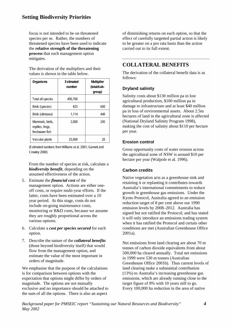
focus is not intended to be on threatened species per se. Rather, the numbers of threatened species have been used to indicate the relative strength of the threatening process that each management option mitigates. The derivation of the multipliers and their values is shown in the table below.

Organisms Estimated number

Multiplier (total/sub-

group)

Total all species 490,700

Birds (species) 825 600

Birds (ultrataxa) 1,114 440

Mammals, birds, reptiles, frogs, freshwater fish

2,000 245

Vascular plants 25,000 20

(Estimated numbers from Williams et al. 2001; Garnett and Crowley 2000)

From the number of species at risk, calculate a biodiversity benefit, depending on the assumed effectiveness of the action.

5. Estimate the financial cost of the management option. Actions are either one-off costs, or require multi-year efforts. If the latter, costs have been estimated over a 10 year period. At this stage, costs do not include on-going maintenance costs, monitoring or R&D costs, because we assume they are roughly proportional across the various options.

6. Calculate a cost per species secured for each option.

7. Describe the nature of the collateral benefits (those beyond biodiversity itself) that would flow from the management option, and estimate the value of the most important in orders of magnitude.

We emphasise that the purpose of the calculations is for comparison between options with the expectation that options might differ by orders of magnitude. The options are not mutually exclusive and no importance should be attached to the sum of all the options. There is also an aspect

of diminishing returns on each option, so that the effect of carefully targetted partial action is likely to be greater on a pro rata basis than the action carried out to its full extent.

COLLATERAL BENEFITS The derivation of the collateral benefit data is as follows:

Dryland salinity Salinity costs about $130 million pa in lost agricultural production, $100 million pa in damage to infrastructure and at least $40 million pa in loss of environmental assets. About 2.5m hectares of land in the agricultural zone is affected (National Dryland Salinity Program 1998), making the cost of salinity about $110 per hectare per year.

Erosion control Gross opportunity costs of water erosion across the agricultural zone of NSW is around $10 per hectare per year (Walpole et al. 1996).

Carbon credits Native vegetation acts as a greenhouse sink and retaining it or replanting it contributes towards Australia’s international commitments to reduce growth in greenhouse gas emissions. Under the Kyoto Protocol, Australia agreed to an emission reduction target of 8 per cent above our 1990 emission levels by 2008–2012. Australia has signed but not ratified the Protocol; and has stated it will only introduce an emissions trading system when it has ratified the Protocol and certain other conditions are met (Australian Greenhouse Office 2001a).

Net emissions from land clearing are about 70 m tonnes of carbon dioxide equivalents from about 500,000 ha cleared annually. Total net emissions in 1999 were 530 m tonnes (Australian Greenhouse Office 2001b). Thus current levels of land clearing make a substantial contribution (13%) to Australia’s increasing greenhouse gas emissions, which are already running close to the target figure of 8% with 10 years still to go. Every 100,000 ha reduction in the area of native



vegetation cleared would lead to a 2.5% improvement in emission performance.

Figures of around $10 per tonne were used in discussions about how an emissions trading system would work. The federal Greenhouse Gas Abatement Program has allocated $400m over three years for large projects that will reduce emissions. Projects were typically allocated about $10m for abatements of around 1.5m tonnes, or about $7 per tonne (Australian Greenhouse Office 2001c). Given that government expects some cost sharing, $10 per tonne seems a reasonable ballpark estimate. Based on the clearing data above, one hectare of land saved from clearing would produce a carbon credit of $1,400.

Clean water The annual costs of water turbidity are estimated as $28m, costs of eutrophication as $200m and costs of sedimentation $4m. Together these make a total of about $230m pa (Land and Water Resources Audit, unpublished data).

River salinity The cost of current levels of salinity in the River Murray system has been estimated as $46m per year (Murray Darling Basin Commission 1999). This includes costs to irrigated agriculture, urban and industrial users, and to the environment.

Water regulation In south-western NSW road damage due to high water tables costs about $9m pa. About 34% of roads and 21%of national highways are affected in this way (National Dryland Salinity Program 1998). Assuming that south-western NSW represents 20% of the area affected across Australia, the national cost would be $45m.

Pollination and honey production 80% of the honey produced in Australia comes from native plants. The gross value of production of the apiary industry is about $60m pa (Gibbs and Muirhead 1998).

However, the value to agriculture (including horticulture) of the paid plus unpaid pollination services of bees and native insects is much larger, about $1.2b pa (Gibbs and Muirhead 1998).

Although honeybees are not native, they largely depend on native vegetation for food while they carry out pollination on agricultural crops (see above). Assume 80% of the $1.2b pa (approx $1b) is due to either native pollinators or food provided to honeybees from native vegetation.

Tourism Australians take about 85,000 day trips per year for holiday/leisure purposes (excluding visiting friends or relatives), spending $7.1b. Another 32,000 overnight trips are made annually with the same purpose, accounting for $17.2b expenditure. International visitors spend a further $8.9b pa (Bureau of Tourism Research 2002). Assuming just 20% of this expenditure involves a visit to a site of natural attraction, that accounts for $6.6b pa.

Value of biodiversity The community’s willingness to pay for improvements in non-market aspects of biodiversity has been estimated by choice modelling as:

• 8c/household for swimming and fishing for every 10 kilometres of degraded waterway that is restored ($259,200/10 km for all Australian households willing to pay), and

• 7c/household for landscape aesthetics for every 10,000 ha of farmland rehabilitated ($226,800 for all households, equivalent to $23 per ha). (National Land and Water Resources Audit, unpublished data.)

Regional employment For every 10,000 visitors to a regional national park in NSW, some 4 and 7 local jobs are generated and regional business turnover is increased by some $130,000 to $270,000 (Gillespie 2000). The choice modelling referred to above found that households put a value of 9c on every 10 people retained in rural areas.

The environmental management industry is expanding. An ASTEC report estimated that if Australia could capture just 2 per cent of the anticipated world pollution market in 2010, 150,000 jobs and $8 billion in business would be



generated (Australian Science, Technology and Engineering Council 1996).

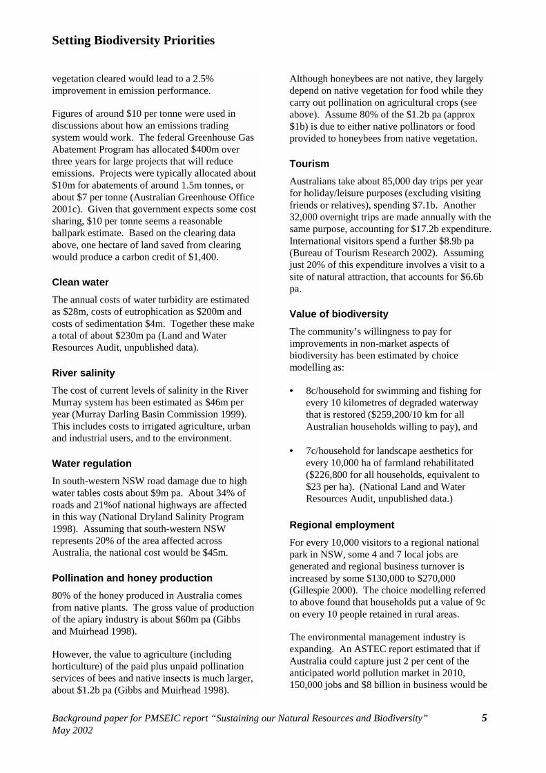
SUMMARY TABLE OF COLLATERAL BENEFITS

Collateral benefit Estimate of value

Dryland salinity $110 per ha pa

Soil erosion $10 per ha pa

Carbon sink $1,400 per ha bush

Clean water $230m pa

River salinity $46m pa

Water regulation Road damage - $45m pa

Pollination $1b pa

Tourism $6.6b pa total

River recreation $259,200 per 10 km river

Landscape aesthetics $226,800 per 10,000 ha

The calculation of collateral benefits for each option is limited to those with the largest order of magnitude, on the basis that adding benefits of much smaller value will have an insignificant impact on the total. We also acknowledge that collateral benefits may not be strictly additive.

MANAGEMENT OPTIONS

1. Clearing and habitat fragmentation Current risk Native vegetation management is a major issue for Australia’s biodiversity, with the extent of woody vegetation currently less than half that prior to white settlement (Barson et al. 2000). Land clearing, particularly in Queensland has attracted recent political attention, and legislation protecting vegetation from clearing varies across states.

Objective Protect and restore native vegetation and terrestrial ecosystems. [NOTBC 1]

Reverse the long term decline in the quality and extent of Australia’s native vegetation and ecological communities and the ecosystem services they provide. [NOTBC 1.1]

o Stop clearing of ecological communities below 30% of their pre-1750 extent. [NOTBC 1.1.2]

o Achieve zero net national rate of land clearance. [NOTBC 1.1.4]

Protect a representative sample of Australia’s terrestrial ecosystems. [NOTBC 1.2]

o By 2005, a representative sample of each bioregion … is protected within the National Reserve System or network of Indigenous Protected Areas or as private land managed for conservation under a conservation agreement. [NOTBC 1.2.3]

o Restore communities below 10% of their pre-1750 levels to that benchmark. [NOTBC 1.2.4]

Some management options A. Prevent broadscale clearing of communities of

high biodiversity value in Queensland

B. Prevent broadscale clearing of ecological communities in the Murray Darling Basin that have high multiple ecosystem service values

C. Restore ecological communities that have fallen below 10 % back to 10% of their original area, in the 5 IBRA regions that have <30% native vegetation remaining.

D. Restore native vegetation in all IBRA sub-regions that have fallen below 10% back to 10% of their original area. (A variation on C.)

E. Consolidate the National Reserve System to achieve comprehensiveness targets.

Costs and benefits

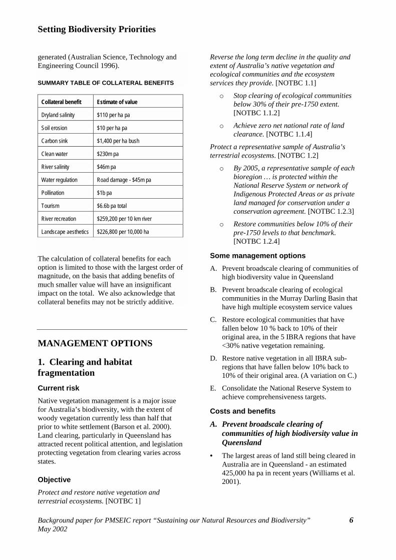
A. Prevent broadscale clearing of communities of high biodiversity value in Queensland

• The largest areas of land still being cleared in Australia are in Queensland - an estimated 425,000 ha pa in recent years (Williams et al. 2001).



• There are 1,085 regional ecosystems defined for Queensland in the “of concern” category – those with 10-30% of pre-clearing extent, plus those with >30% but remnant area is small (<10,000 ha). There are 2,270,400 ha in the “of concern” category (Fensham and Sattler, unpublished data).

• The Queensland government has calculated it needs $200m to compensate landowners for not clearing the “of concern” area.

• Additional costs could be incurred in the future if the same approach were taken with areas currently ‘not of concern’ but that reach the 30% threshold as clearing for development continues. These costs are not included in these calculations.

• 12 bird taxa (ultrataxa) are extinct or threatened by clearing in rainforest and tropical and sub-tropical woodland (Garnett and Crowley 2000), vegetation types most represented in ‘of concern’ ecosystems.

• Using the ultrataxa multiplier (440), this action would prevent 5,280 species becoming threatened.

• The collateral benefit would be predominantly in carbon credits and prevention of erosion and salinity. At $1,400 per ha, carbon credits would contribute $3,178m. Assuming a third of the area is susceptible to salinity, prevention of salinity would be valued at $830m over a 10 year period. The total is $4,008m.

Factor Value

No. of species saved 5,280

Area 2,270,400 ha

Cost/ha $88

Total cost $200m

No. species saved/$1m 26

Collateral benefit $4,008m

Collateral benefit/total cost 20

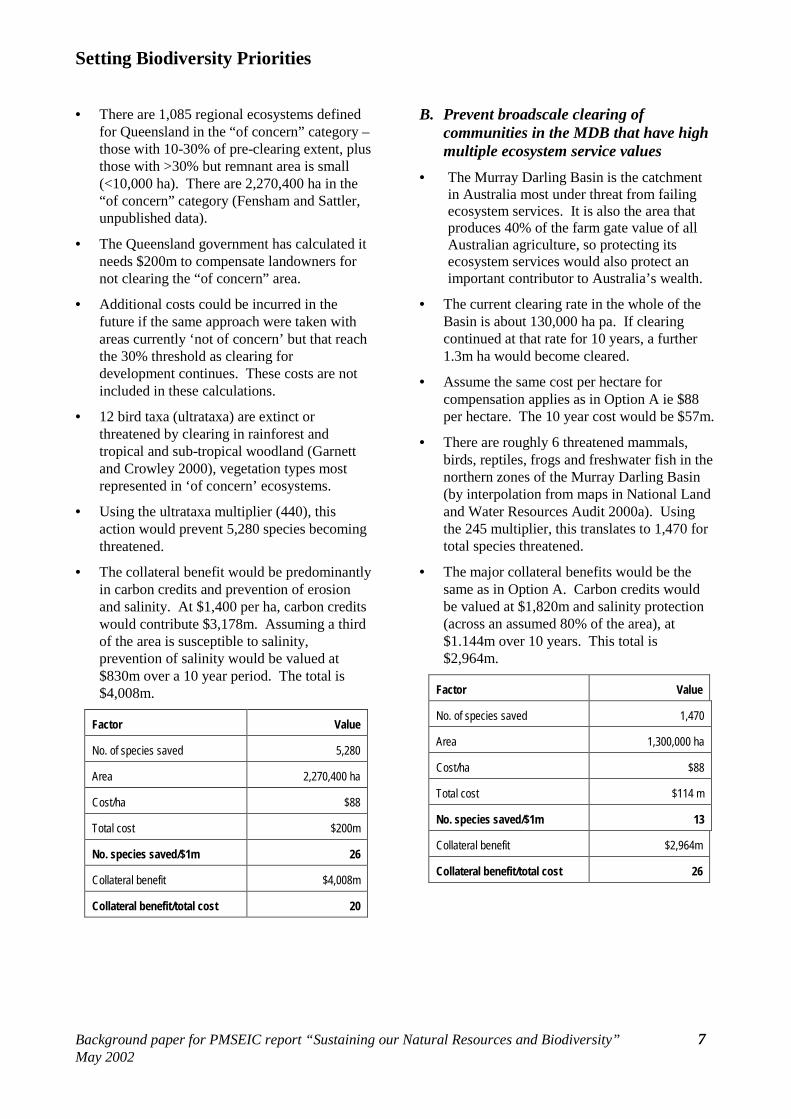
B. Prevent broadscale clearing of communities in the MDB that have high multiple ecosystem service values

• The Murray Darling Basin is the catchment in Australia most under threat from failing ecosystem services. It is also the area that produces 40% of the farm gate value of all Australian agriculture, so protecting its ecosystem services would also protect an important contributor to Australia’s wealth.

• The current clearing rate in the whole of the Basin is about 130,000 ha pa. If clearing continued at that rate for 10 years, a further 1.3m ha would become cleared.

• Assume the same cost per hectare for compensation applies as in Option A ie $88 per hectare. The 10 year cost would be $57m.

• There are roughly 6 threatened mammals, birds, reptiles, frogs and freshwater fish in the northern zones of the Murray Darling Basin (by interpolation from maps in National Land and Water Resources Audit 2000a). Using the 245 multiplier, this translates to 1,470 for total species threatened.

• The major collateral benefits would be the same as in Option A. Carbon credits would be valued at $1,820m and salinity protection (across an assumed 80% of the area), at $1.144m over 10 years. This total is $2,964m.

Factor Value


Area 1,300,000 ha

Cost/ha $88

Total cost $114 m






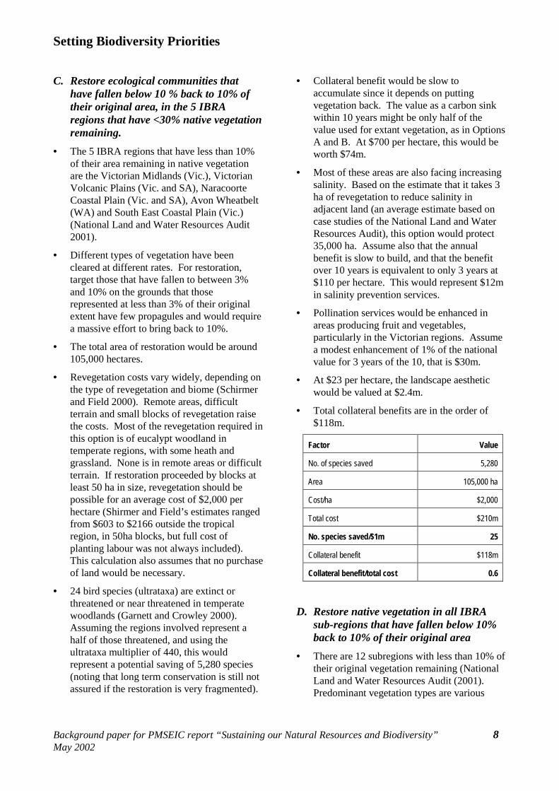
C. Restore ecological communities that have fallen below 10 % back to 10% of their original area, in the 5 IBRA regions that have <30% native vegetation remaining.

• The 5 IBRA regions that have less than 10% of their area remaining in native vegetation are the Victorian Midlands (Vic.), Victorian Volcanic Plains (Vic. and SA), Naracoorte Coastal Plain (Vic. and SA), Avon Wheatbelt (WA) and South East Coastal Plain (Vic.) (National Land and Water Resources Audit 2001).

• Different types of vegetation have been cleared at different rates. For restoration, target those that have fallen to between 3% and 10% on the grounds that those represented at less than 3% of their original extent have few propagules and would require a massive effort to bring back to 10%.

• The total area of restoration would be around 105,000 hectares.

• Revegetation costs vary widely, depending on the type of revegetation and biome (Schirmer and Field 2000). Remote areas, difficult terrain and small blocks of revegetation raise the costs. Most of the revegetation required in this option is of eucalypt woodland in temperate regions, with some heath and grassland. None is in remote areas or difficult terrain. If restoration proceeded by blocks at least 50 ha in size, revegetation should be possible for an average cost of $2,000 per hectare (Shirmer and Field’s estimates ranged from $603 to $2166 outside the tropical region, in 50ha blocks, but full cost of planting labour was not always included). This calculation also assumes that no purchase of land would be necessary.

• 24 bird species (ultrataxa) are extinct or threatened or near threatened in temperate woodlands (Garnett and Crowley 2000). Assuming the regions involved represent a half of those threatened, and using the ultrataxa multiplier of 440, this would represent a potential saving of 5,280 species (noting that long term conservation is still not assured if the restoration is very fragmented).

• Collateral benefit would be slow to accumulate since it depends on putting vegetation back. The value as a carbon sink within 10 years might be only half of the value used for extant vegetation, as in Options A and B. At $700 per hectare, this would be worth $74m.

• Most of these areas are also facing increasing salinity. Based on the estimate that it takes 3 ha of revegetation to reduce salinity in adjacent land (an average estimate based on case studies of the National Land and Water Resources Audit), this option would protect 35,000 ha. Assume also that the annual benefit is slow to build, and that the benefit over 10 years is equivalent to only 3 years at $110 per hectare. This would represent $12m in salinity prevention services.

• Pollination services would be enhanced in areas producing fruit and vegetables, particularly in the Victorian regions. Assume a modest enhancement of 1% of the national value for 3 years of the 10, that is $30m.

• At $23 per hectare, the landscape aesthetic would be valued at $2.4m.

• Total collateral benefits are in the order of $118m.

Factor Value


Area 105,000 ha

Cost/ha $2,000

Total cost $210m


Collateral benefit $118m

Collateral benefit/total cost 0.6

D. Restore native vegetation in all IBRA sub-regions that have fallen below 10% back to 10% of their original area

• There are 12 subregions with less than 10% of their original vegetation remaining (National Land and Water Resources Audit (2001). Predominant vegetation types are various



forms of eucalypt woodlands and mallee shrublands.

• These subregions are listed as having between 0-10% native vegetation (more precise values for each sub-region should be available soon). Assume the average remaining is 5%.

• As in the example above, assume communities present at 3% or less to be too inefficient to restore. Effectively this reduces the target on an area basis from 10% to 7%.

• Restoration would therefore involve some 200,000 hectares (restoration from 5% to 7% of 10m hectares.)

• Assume restoration costs of $2,000 per ha, as in the previous example.

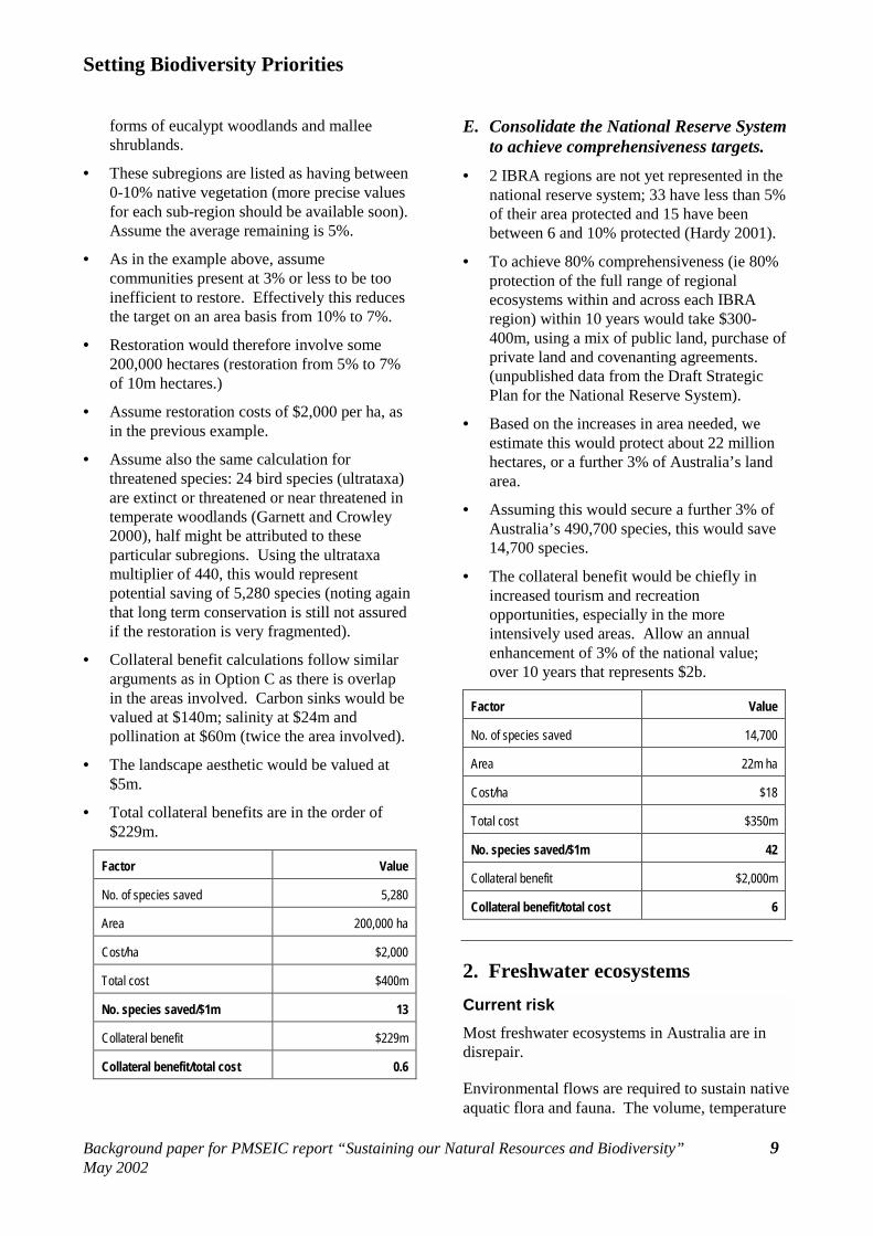
• Assume also the same calculation for threatened species: 24 bird species (ultrataxa) are extinct or threatened or near threatened in temperate woodlands (Garnett and Crowley 2000), half might be attributed to these particular subregions. Using the ultrataxa multiplier of 440, this would represent potential saving of 5,280 species (noting again that long term conservation is still not assured if the restoration is very fragmented).

• Collateral benefit calculations follow similar arguments as in Option C as there is overlap in the areas involved. Carbon sinks would be valued at $140m; salinity at $24m and pollination at $60m (twice the area involved).

• The landscape aesthetic would be valued at $5m.

• Total collateral benefits are in the order of $229m.

Factor Value


Area 200,000 ha

Cost/ha $2,000

Total cost $400m




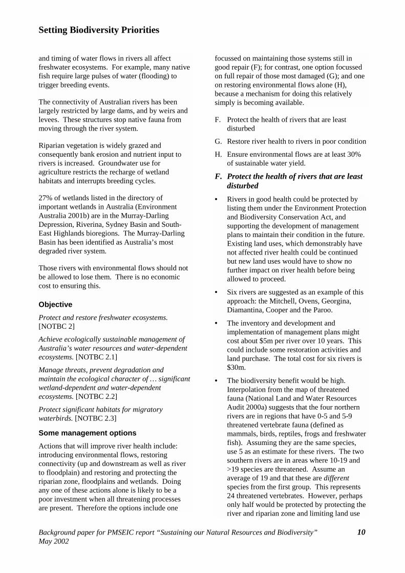
E. Consolidate the National Reserve System to achieve comprehensiveness targets.

• 2 IBRA regions are not yet represented in the national reserve system; 33 have less than 5% of their area protected and 15 have been between 6 and 10% protected (Hardy 2001).

• To achieve 80% comprehensiveness (ie 80% protection of the full range of regional ecosystems within and across each IBRA region) within 10 years would take $300-400m, using a mix of public land, purchase of private land and covenanting agreements. (unpublished data from the Draft Strategic Plan for the National Reserve System).

• Based on the increases in area needed, we estimate this would protect about 22 million hectares, or a further 3% of Australia’s land area.

• Assuming this would secure a further 3% of Australia’s 490,700 species, this would save 14,700 species.

• The collateral benefit would be chiefly in increased tourism and recreation opportunities, especially in the more intensively used areas. Allow an annual enhancement of 3% of the national value; over 10 years that represents $2b.

Factor Value


Area 22m ha

Cost/ha $18

Total cost $350m




2. Freshwater ecosystems Current risk Most freshwater ecosystems in Australia are in disrepair.

Environmental flows are required to sustain native aquatic flora and fauna. The volume, temperature



and timing of water flows in rivers all affect freshwater ecosystems. For example, many native fish require large pulses of water (flooding) to trigger breeding events.

The connectivity of Australian rivers has been largely restricted by large dams, and by weirs and levees. These structures stop native fauna from moving through the river system.

Riparian vegetation is widely grazed and consequently bank erosion and nutrient input to rivers is increased. Groundwater use for agriculture restricts the recharge of wetland habitats and interrupts breeding cycles.

27% of wetlands listed in the directory of important wetlands in Australia (Environment Australia 2001b) are in the Murray-Darling Depression, Riverina, Sydney Basin and South-East Highlands bioregions. The Murray-Darling Basin has been identified as Australia’s most degraded river system.

Those rivers with environmental flows should not be allowed to lose them. There is no economic cost to ensuring this.

Objective Protect and restore freshwater ecosystems. [NOTBC 2]

Achieve ecologically sustainable management of Australia’s water resources and water-dependent ecosystems. [NOTBC 2.1]

Manage threats, prevent degradation and maintain the ecological character of … significant wetland-dependent and water-dependent ecosystems. [NOTBC 2.2]

Protect significant habitats for migratory waterbirds. [NOTBC 2.3]

Some management options Actions that will improve river health include: introducing environmental flows, restoring connectivity (up and downstream as well as river to floodplain) and restoring and protecting the riparian zone, floodplains and wetlands. Doing any one of these actions alone is likely to be a poor investment when all threatening processes are present. Therefore the options include one

focussed on maintaining those systems still in good repair (F); for contrast, one option focussed on full repair of those most damaged (G); and one on restoring environmental flows alone (H), because a mechanism for doing this relatively simply is becoming available.

F. Protect the health of rivers that are least disturbed

G. Restore river health to rivers in poor condition

H. Ensure environmental flows are at least 30% of sustainable water yield.

F. Protect the health of rivers that are least disturbed

• Rivers in good health could be protected by listing them under the Environment Protection and Biodiversity Conservation Act, and supporting the development of management plans to maintain their condition in the future. Existing land uses, which demonstrably have not affected river health could be continued but new land uses would have to show no further impact on river health before being allowed to proceed.

• Six rivers are suggested as an example of this approach: the Mitchell, Ovens, Georgina, Diamantina, Cooper and the Paroo.

• The inventory and development and implementation of management plans might cost about $5m per river over 10 years. This could include some restoration activities and land purchase. The total cost for six rivers is $30m.

• The biodiversity benefit would be high. Interpolation from the map of threatened fauna (National Land and Water Resources Audit 2000a) suggests that the four northern rivers are in regions that have 0-5 and 5-9 threatened vertebrate fauna (defined as mammals, birds, reptiles, frogs and freshwater fish). Assuming they are the same species, use 5 as an estimate for these rivers. The two southern rivers are in areas where 10-19 and >19 species are threatened. Assume an average of 19 and that these are different species from the first group. This represents 24 threatened vertebrates. However, perhaps only half would be protected by protecting the river and riparian zone and limiting land use



change in the catchment. This would mean 12 vertebrates would be protected. Using the appropriate multiplier of 245, this represents 2,940 species.

• Collateral benefit would be in avoidance of future costs of degradation to water quality. However, these rivers are not in areas heavily prone to dryland salinity, nor are they heavily used for human, industrial or irrigation use. Therefore collateral benefits would primarily be in terms of prevention of sedimentation and eutrophication. These catchments together cover an area about half that of the Murray Darling Basin. Prevention of sedimentation and eutrophication costs to just a third the rate in the Basin would represent a sixth of the current level of $230 pa (assuming most current costs are in the Basin). Over 10 years that represents $380m.

• The Mitchell and Ovens, located in south eastern Australia, would particularly have tourism and recreational value. Over their combined length of about 300km, that represents about $8m, making a total benefit of about $390m.

Factor Value


Total cost $30m




G. Restore river health to rivers in poor condition

• Take the river reaches that have been “extensively” and “substantially” modified according to the river environment index calculated for the National Land and Water Resources Audit (National Land and Water Resources Audit 2002, yet to be released). Their length is 36,600km, representing 20% of total river reach in Australia.

• Assuming these are the river reaches that are most over-committed in water allocation, purchase of environmental flows would be required. Assuming water yield is distributed

evenly along all rivers, 20% of the national sustainable yield is about 3.8m ML. Assume also that on average these reaches are 20% over-allocated and that a target of 15% of sustainable yield is desired for environmental flows. The cost of purchasing 35% of sustainable flows at $1,000/ML would be about $3.3b.

• There are some 1,700 barriers to fish movement on rivers in the Murray-Darling Basin in NSW and 2,500 throughout Victoria (Ball et al. 2001). Say there are 5,000 for the nation, but that three-quarters of them are in this 20% of extensively modified reaches ie 3,750. Removing a third of the barriers (say 1,200) might be a realistic goal that would still allow harvest of water for human use. It costs about $100,000 to remove a barrier and deal satisfactorily with the accumulated sediment. Removing 1,200 would therefore cost $120m.

• Fencing 50% of both sides of the 36,600km of river length to protect riparian vegetation would cost $73m, at $2,000/km (assume some already fenced, some is inaccessible and some not at threat from grazing).

• Fish ladders or lifts cost around $500,000 to install on small to medium weirs. Installing fish ladders at a third of the barriers (1,200 places) would cost $600m. (If one third of the barriers are removed, this effectively places fish ladders on half those remaining.)

• Reducing floodplain isolation by removing a proportion of levee banks would be part of this package. There is no estimate of the length of levees in Australia. Allow $50m.

• Total costs would be $4,143m.

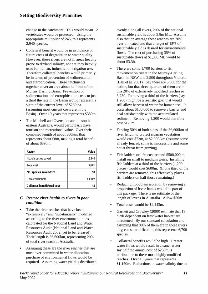
• Garnett and Crowley (2000) estimate that 19 birds dependent on freshwater habitat are threatened. By our standard calculation and assuming that 80% of them are in these rivers of greatest modification, this represents 6,700 species.

• Collateral benefits would be high. Greater water flows would result in cleaner water – say half the annual cost of $230m is attributable to these most highly modified reaches. Over 10 years that represents $1,150m. Reductions in water salinity due to



greater flushing might realise 10% of the annual cost of $46m, equivalent to $46m over 10 years. River recreation values would increase, say over a quarter of the river length. At $260,000 per 10 km river, this represents $60m. The total for these items is $1,256m.

Factor Value


Total cost $4,143 m


Collateral benefit $1,256


H. Ensure environmental flows are at least

15% of sustainable water yield. • The market for water rights provides a

relatively simple national mechanism to increase the environmental flows in rivers that are currently highly allocated to other uses.

• The Murray Darling Basin is the river system most heavily used. Based on returning 15% of the sustainable yield of the Murray Darling Basin (9,127 GL, National Land and Water Resources Audit 2000c) to environmental flows, from a base of 20% over-allocation, and buying water at $1,000 per ML, would cost around $3.2b. (Small purchases in other systems would have little impact on this total.)

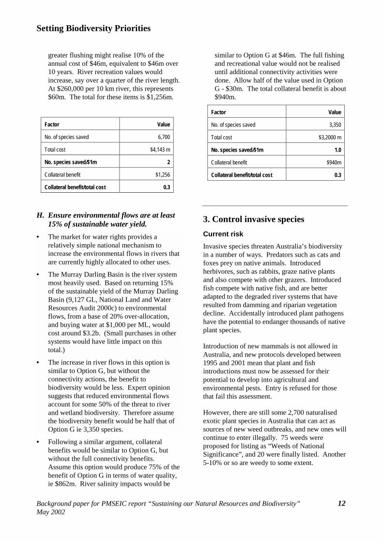
• The increase in river flows in this option is similar to Option G, but without the connectivity actions, the benefit to biodiversity would be less. Expert opinion suggests that reduced environmental flows account for some 50% of the threat to river and wetland biodiversity. Therefore assume the biodiversity benefit would be half that of Option G ie 3,350 species.

• Following a similar argument, collateral benefits would be similar to Option G, but without the full connectivity benefits. Assume this option would produce 75% of the benefit of Option G in terms of water quality, ie $862m. River salinity impacts would be

similar to Option G at $46m. The full fishing and recreational value would not be realised until additional connectivity activities were done. Allow half of the value used in Option G - $30m. The total collateral benefit is about $940m.

Factor Value


Total cost $3,2000 m

No. species saved/$1m 1.0



3. Control invasive species Current risk Invasive species threaten Australia’s biodiversity in a number of ways. Predators such as cats and foxes prey on native animals. Introduced herbivores, such as rabbits, graze native plants and also compete with other grazers. Introduced fish compete with native fish, and are better adapted to the degraded river systems that have resulted from damming and riparian vegetation decline. Accidentally introduced plant pathogens have the potential to endanger thousands of native plant species.

Introduction of new mammals is not allowed in Australia, and new protocols developed between 1995 and 2001 mean that plant and fish introductions must now be assessed for their potential to develop into agricultural and environmental pests. Entry is refused for those that fail this assessment.

However, there are still some 2,700 naturalised exotic plant species in Australia that can act as sources of new weed outbreaks, and new ones will continue to enter illegally. 75 weeds were proposed for listing as “Weeds of National Significance”, and 20 were finally listed. Another 5-10% or so are weedy to some extent.



The fungal disease Phytophthora, mostly P. cinnamomi but other species are also involved, is a serious spreading threat to native vegetation, particularly woodland, forest and heathland. Some important iconic plants are highly susceptible, plants like eucalypts, banksias and grevilleas.

Objective Control invasive species. [NOTBC 4]

Prevent or control the introduction and spread of feral animals and weed species. [NOTBC 4.1]

The working party added “and introduced fungal diseases.”

Some management options I. Limit the spread of Phytophthora

J. Eradicate new outbreaks of naturalised plant species with weedy potential

K. Biological control of weeds of national significance

L. Mechanical and herbicidal control of weeds

M. Biological control of vertebrate pests

N. Mechanical control of feral predators

Costs and benefits

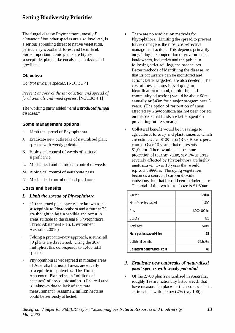
I. Limit the spread of Phytophthora • 31 threatened plant species are known to be

susceptible to Phytophthora and a further 39 are thought to be susceptible and occur in areas suitable to the disease (Phytophthora Threat Abatement Plan, Environment Australia 2001c).

• Taking a precautionary approach, assume all 70 plants are threatened. Using the 20x multiplier, this corresponds to 1,400 total species.

• Phytophthora is widespread in moister areas of Australia but not all areas are equally susceptible to epidemics. The Threat Abatement Plan refers to “millions of hectares” of broad infestation. (The real area is unknown due to lack of accurate measurement.) Assume 2 million hectares could be seriously affected.

• There are no eradication methods for Phytophthora. Limiting the spread to prevent future damage is the most cost-effective management action. This depends primarily on gaining the cooperation of governments, landowners, industries and the public in following strict soil hygiene procedures. Better methods of identifying the disease, so that its occurrence can be monitored and actions better targetted, are also needed. The cost of these actions (developing an identification method, monitoring and community education) would be about $8m annually or $40m for a major program over 5 years. (The option of restoration of areas affected by Phytophthora has not been costed on the basis that funds are better spent on preventing future spread.)

• Collateral benefit would be in savings to agriculture, forestry and plant nurseries which are estimated as $100m pa (Rick Roush, pers. com.). Over 10 years, that represents $1,000m. There would also be some protection of tourism value, say 1% as areas severely affected by Phytophthora are highly unattractive. Over 10 years that would represent $660m. The dying vegetation becomes a source of carbon dioxide emissions, but that hasn’t been included here. The total of the two items above is $1,600m.

Factor Value


Area 2,000,000 ha

Cost/ha $20

Total cost $40m




J. Eradicate new outbreaks of naturalised plant species with weedy potential

• Of the 2,700 plants naturalised in Australia, roughly 1% are nationally listed weeds that have measures in place for their control. This action deals with the next 4% (say 100) -



those that have the potential to be weedy to some extent.

• Some 4-10 plant species are at risk from every serious weed (Rick Roush, pers. com.). Assume a lower estimate of six for these somewhat less weedy species, leading to 600 plants at risk from 100 weeds. On the basis that weeds have a less devastating impact on whole habitats than threats like clearing, fragmentation, salinity etc, use half the plant multiplier (0.5 x 20) to reach total species. This equates to 6,000 total species.

• For comparison, Garnett and Crowley (2000) estimate 16 birds are threatened or vulnerable due to weeds. Using the bird multiplier (at full strength), the estimate would be 9,600 species. This is within the same order of magnitude but to be conservative, we’ll use the lower figure.

• The Northern Australia Quarantine Strategy (NAQS) locates and eradicates on average two newly naturalised plant species per year in the NT and northern areas of WA and Queensland. The program costs $3.6m per year..

• Assume that a similar activity in southern Australia would cost the same (larger area, but much more accessible), so the two programs together would cost $7.2m annually. Over ten years that is equivalent to $72m.

• Collateral benefits are difficult to estimate since the actual species and their impacts are not known. Perhaps 10% of the collateral benefit of Option K (below), which is based on the most assertive weeds, would be reasonable, that is $100m.

Factor Value


Area 670m ha

Cost/ha $0.11

Total cost $72m




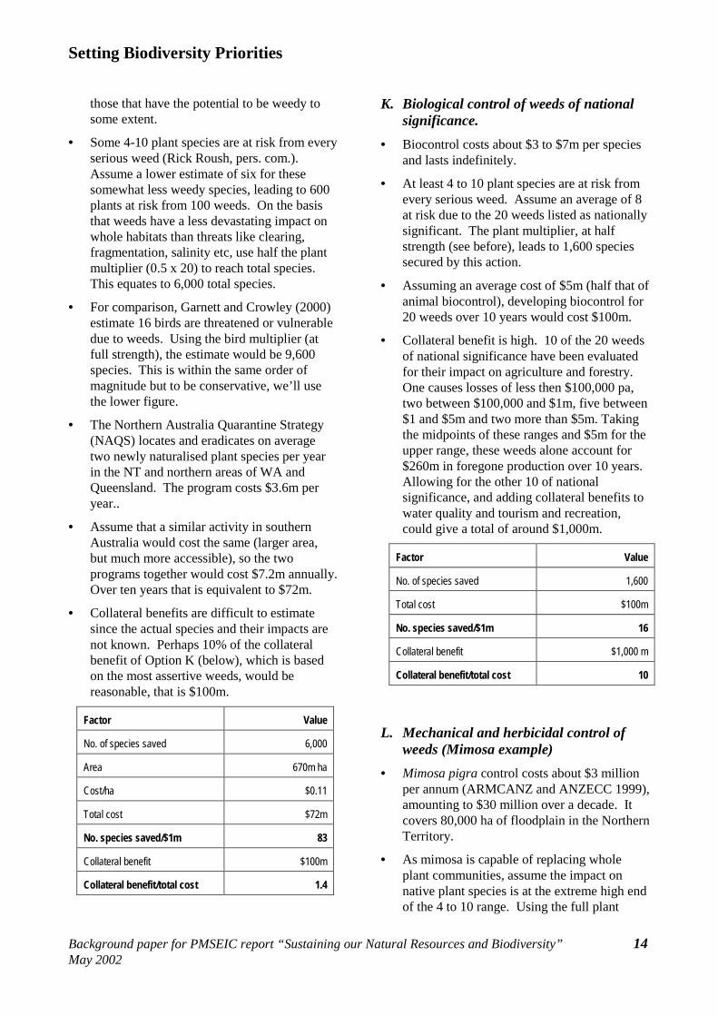
K. Biological control of weeds of national significance.

• Biocontrol costs about $3 to $7m per species and lasts indefinitely.

• At least 4 to 10 plant species are at risk from every serious weed. Assume an average of 8 at risk due to the 20 weeds listed as nationally significant. The plant multiplier, at half strength (see before), leads to 1,600 species secured by this action.

• Assuming an average cost of $5m (half that of animal biocontrol), developing biocontrol for 20 weeds over 10 years would cost $100m.

• Collateral benefit is high. 10 of the 20 weeds of national significance have been evaluated for their impact on agriculture and forestry. One causes losses of less then $100,000 pa, two between $100,000 and $1m, five between $1 and $5m and two more than $5m. Taking the midpoints of these ranges and $5m for the upper range, these weeds alone account for $260m in foregone production over 10 years. Allowing for the other 10 of national significance, and adding collateral benefits to water quality and tourism and recreation, could give a total of around $1,000m.

Factor Value


Total cost $100m


Collateral benefit $1,000 m


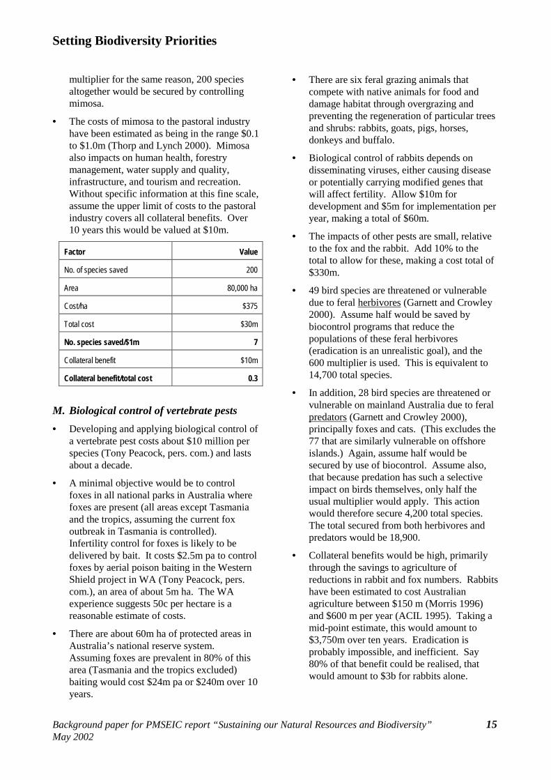
L. Mechanical and herbicidal control of weeds (Mimosa example)

• Mimosa pigra control costs about $3 million per annum (ARMCANZ and ANZECC 1999), amounting to $30 million over a decade. It covers 80,000 ha of floodplain in the Northern Territory.

• As mimosa is capable of replacing whole plant communities, assume the impact on native plant species is at the extreme high end of the 4 to 10 range. Using the full plant



multiplier for the same reason, 200 species altogether would be secured by controlling mimosa.

• The costs of mimosa to the pastoral industry have been estimated as being in the range $0.1 to $1.0m (Thorp and Lynch 2000). Mimosa also impacts on human health, forestry management, water supply and quality, infrastructure, and tourism and recreation. Without specific information at this fine scale, assume the upper limit of costs to the pastoral industry covers all collateral benefits. Over 10 years this would be valued at $10m.

Factor Value

No. of species saved 200

Area 80,000 ha

Cost/ha $375

Total cost $30m




M. Biological control of vertebrate pests • Developing and applying biological control of

a vertebrate pest costs about $10 million per species (Tony Peacock, pers. com.) and lasts about a decade.

• A minimal objective would be to control foxes in all national parks in Australia where foxes are present (all areas except Tasmania and the tropics, assuming the current fox outbreak in Tasmania is controlled). Infertility control for foxes is likely to be delivered by bait. It costs $2.5m pa to control foxes by aerial poison baiting in the Western Shield project in WA (Tony Peacock, pers. com.), an area of about 5m ha. The WA experience suggests 50c per hectare is a reasonable estimate of costs.

• There are about 60m ha of protected areas in Australia’s national reserve system. Assuming foxes are prevalent in 80% of this area (Tasmania and the tropics excluded) baiting would cost $24m pa or $240m over 10 years.

• There are six feral grazing animals that compete with native animals for food and damage habitat through overgrazing and preventing the regeneration of particular trees and shrubs: rabbits, goats, pigs, horses, donkeys and buffalo.

• Biological control of rabbits depends on disseminating viruses, either causing disease or potentially carrying modified genes that will affect fertility. Allow $10m for development and $5m for implementation per year, making a total of $60m.

• The impacts of other pests are small, relative to the fox and the rabbit. Add 10% to the total to allow for these, making a cost total of $330m.

• 49 bird species are threatened or vulnerable due to feral herbivores (Garnett and Crowley 2000). Assume half would be saved by biocontrol programs that reduce the populations of these feral herbivores (eradication is an unrealistic goal), and the 600 multiplier is used. This is equivalent to 14,700 total species.

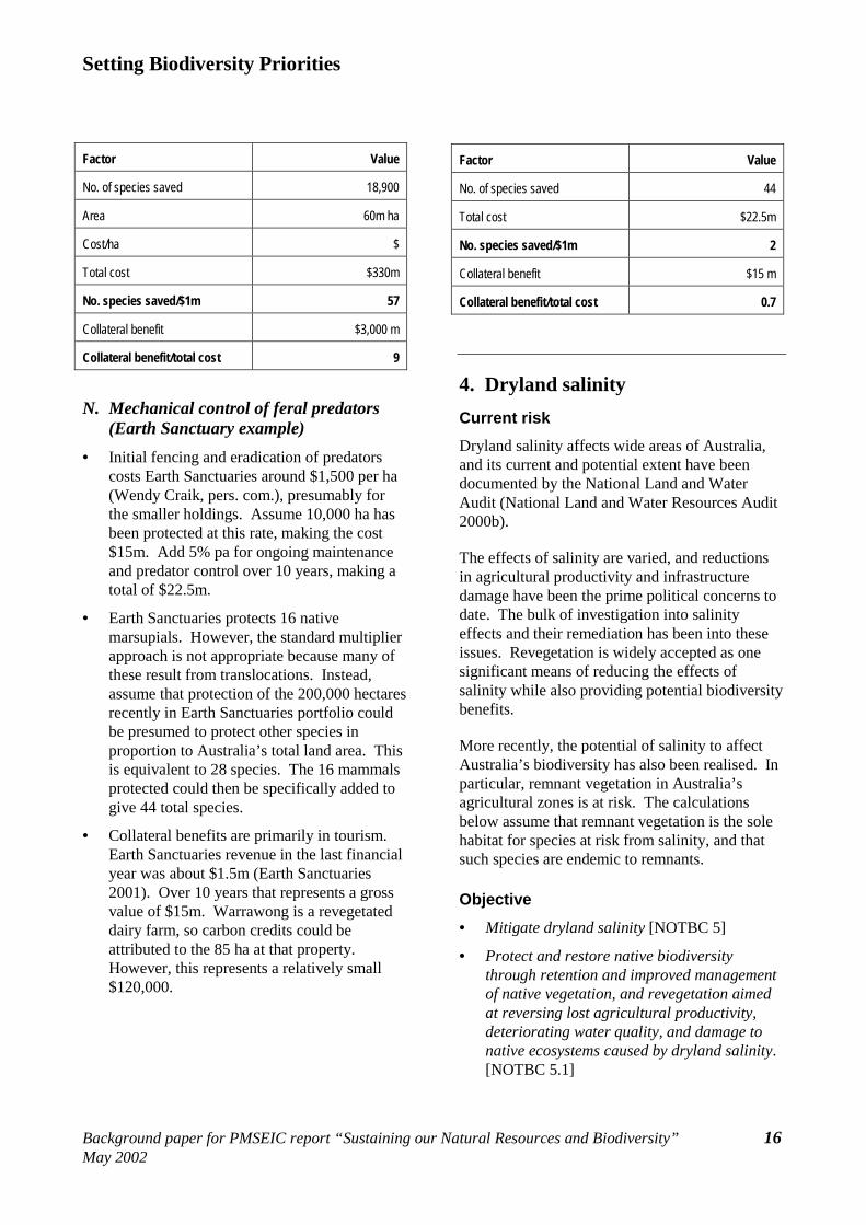
• In addition, 28 bird species are threatened or vulnerable on mainland Australia due to feral predators (Garnett and Crowley 2000), principally foxes and cats. (This excludes the 77 that are similarly vulnerable on offshore islands.) Again, assume half would be secured by use of biocontrol. Assume also, that because predation has such a selective impact on birds themselves, only half the usual multiplier would apply. This action would therefore secure 4,200 total species. The total secured from both herbivores and predators would be 18,900.

• Collateral benefits would be high, primarily through the savings to agriculture of reductions in rabbit and fox numbers. Rabbits have been estimated to cost Australian agriculture between $150 m (Morris 1996) and $600 m per year (ACIL 1995). Taking a mid-point estimate, this would amount to $3,750m over ten years. Eradication is probably impossible, and inefficient. Say 80% of that benefit could be realised, that would amount to $3b for rabbits alone.



Factor Value


Area 60m ha

Cost/ha $

Total cost $330m


Collateral benefit $3,000 m


N. Mechanical control of feral predators (Earth Sanctuary example)

• Initial fencing and eradication of predators costs Earth Sanctuaries around $1,500 per ha (Wendy Craik, pers. com.), presumably for the smaller holdings. Assume 10,000 ha has been protected at this rate, making the cost $15m. Add 5% pa for ongoing maintenance and predator control over 10 years, making a total of $22.5m.

• Earth Sanctuaries protects 16 native marsupials. However, the standard multiplier approach is not appropriate because many of these result from translocations. Instead, assume that protection of the 200,000 hectares recently in Earth Sanctuaries portfolio could be presumed to protect other species in proportion to Australia’s total land area. This is equivalent to 28 species. The 16 mammals protected could then be specifically added to give 44 total species.

• Collateral benefits are primarily in tourism. Earth Sanctuaries revenue in the last financial year was about $1.5m (Earth Sanctuaries 2001). Over 10 years that represents a gross value of $15m. Warrawong is a revegetated dairy farm, so carbon credits could be attributed to the 85 ha at that property. However, this represents a relatively small $120,000.

Factor Value


Total cost $22.5m


Collateral benefit $15 m


4. Dryland salinity Current risk Dryland salinity affects wide areas of Australia, and its current and potential extent have been documented by the National Land and Water Audit (National Land and Water Resources Audit 2000b).

The effects of salinity are varied, and reductions in agricultural productivity and infrastructure damage have been the prime political concerns to date. The bulk of investigation into salinity effects and their remediation has been into these issues. Revegetation is widely accepted as one significant means of reducing the effects of salinity while also providing potential biodiversity benefits.

More recently, the potential of salinity to affect Australia’s biodiversity has also been realised. In particular, remnant vegetation in Australia’s agricultural zones is at risk. The calculations below assume that remnant vegetation is the sole habitat for species at risk from salinity, and that such species are endemic to remnants.

Objective • Mitigate dryland salinity [NOTBC 5]

• Protect and restore native biodiversity through retention and improved management of native vegetation, and revegetation aimed at reversing lost agricultural productivity, deteriorating water quality, and damage to native ecosystems caused by dryland salinity. [NOTBC 5.1]



Some management options O. Strategic revegetation to prevent salinity from

further affecting remnant vegetation

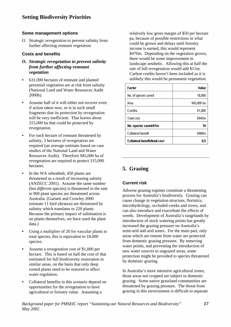
Costs and benefits O. Strategic revegetation to prevent salinity

from further affecting remnant vegetation

• 631,000 hectares of remnant and planted perennial vegetation are at risk from salinity (National Land and Water Resources Audit 2000b).

• Assume half of it will either not recover even if action taken now, or is in such small fragments that its protection by revegetation will be very inefficient. That leaves about 315,000 ha that could be protected by revegetation.

• For each hectare of remnant threatened by salinity, 3 hectares of revegetation are required (an average estimate based on case studies of the National Land and Water Resources Audit). Therefore 945,000 ha of revegetation are required to protect 315,000 hectares.

• In the WA wheatbelt, 450 plants are threatened as a result of increasing salinity (ANZECC 2001). Assume the same number (but different species) is threatened in the east ie 900 plant species are threatened across Australia. (Garnett and Crowley 2000 estimate 11 bird ultrataxa are threatened by salinity which translates to 220 plants. Because the primary impact of salinisation is on plants themselves, we have used the plant data.)

• Using a multiplier of 20 for vascular plants to total species, this is equivalent to 18,000 species.

• Assume a revegetation cost of $1,000 per hectare. This is based on half the cost of that estimated for full biodiversity restoration in similar areas, on the basis that only deep rooted plants need to be restored to affect water regulation.

• Collateral benefits in this scenario depend on opportunities for the revegetation to have agricultural or forestry value. Assuming a

relatively low gross margin of $50 per hectare pa, because of possible restrictions in what could be grown and delays until forestry income is earned, this would represent $470m. Depending on the vegetation grown, there would be some improvement in landscape aesthetic. Allowing this at half the rate of full revegetation would add $11m. Carbon credits haven’t been included as it is unlikely this would be permanent vegetation.

Factor Value


Area 945,000 ha

Cost/ha $1,000

Total cost $945m




5. Grazing Current risk Adverse grazing regimes constitute a threatening process for Australia’s biodiversity. Grazing can cause change in vegetation structure, floristics, microhydrology, occluded creeks and rivers, and can also introduce and exacerbate the effects of weeds. Development of Australia’s rangelands by introduction of stock watering points has greatly increased the grazing pressure on Australia’s semi-arid and arid zones. For the main part, only areas which are remote from water are protected from domestic grazing pressure. By removing water points, and preventing the introduction of new water sources to ungrazed areas, some protection might be provided to species threatened by domestic grazing.

In Australia’s more intensive agricultural zones, those areas not cropped are subject to domestic grazing. Some native grassland communities are threatened by grazing pressure. The threat from grazing in this environment is difficult to separate



from the threat presented by reduction in area of grasslands, to allow expansion of cropping or improved pasture establishment. Riparian zones too are at risk, and fencing has been recommended as a way to manage grazing impacts.

Objective Protect areas of high conservation significance at risk of unsustainable grazing pressure. [NOTBC 6.1]

Some management options P. Prevent grazing of 10% of all arid and semi-

arid grazing lands.

Q. Manage grazing for conservation in threatened grasslands in South East Australia

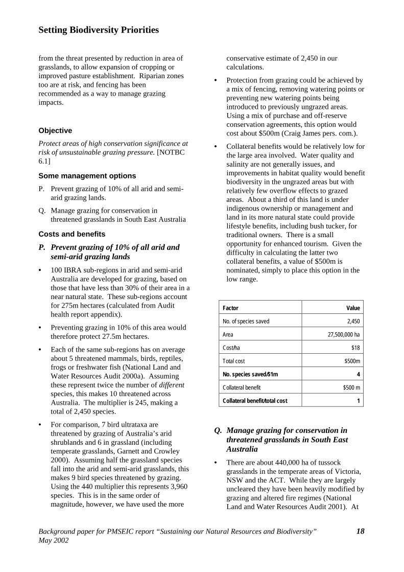
Costs and benefits P. Prevent grazing of 10% of all arid and

semi-arid grazing lands • 100 IBRA sub-regions in arid and semi-arid

Australia are developed for grazing, based on those that have less than 30% of their area in a near natural state. These sub-regions account for 275m hectares (calculated from Audit health report appendix).

• Preventing grazing in 10% of this area would therefore protect 27.5m hectares.

• Each of the same sub-regions has on average about 5 threatened mammals, birds, reptiles, frogs or freshwater fish (National Land and Water Resources Audit 2000a). Assuming these represent twice the number of different species, this makes 10 threatened across Australia. The multiplier is 245, making a total of 2,450 species.

• For comparison, 7 bird ultrataxa are threatened by grazing of Australia’s arid shrublands and 6 in grassland (including temperate grasslands, Garnett and Crowley 2000). Assuming half the grassland species fall into the arid and semi-arid grasslands, this makes 9 bird species threatened by grazing. Using the 440 multiplier this represents 3,960 species. This is in the same order of magnitude, however, we have used the more

conservative estimate of 2,450 in our calculations.

• Protection from grazing could be achieved by a mix of fencing, removing watering points or preventing new watering points being introduced to previously ungrazed areas. Using a mix of purchase and off-reserve conservation agreements, this option would cost about $500m (Craig James pers. com.).

• Collateral benefits would be relatively low for the large area involved. Water quality and salinity are not generally issues, and improvements in habitat quality would benefit biodiversity in the ungrazed areas but with relatively few overflow effects to grazed areas. About a third of this land is under indigenous ownership or management and land in its more natural state could provide lifestyle benefits, including bush tucker, for traditional owners. There is a small opportunity for enhanced tourism. Given the difficulty in calculating the latter two collateral benefits, a value of $500m is nominated, simply to place this option in the low range.

Factor Value


Area 27,500,000 ha

Cost/ha $18

Total cost $500m


Collateral benefit $500 m


Q. Manage grazing for conservation in

threatened grasslands in South East Australia

• There are about 440,000 ha of tussock grasslands in the temperate areas of Victoria, NSW and the ACT. While they are largely uncleared they have been heavily modified by grazing and altered fire regimes (National Land and Water Resources Audit 2001). At



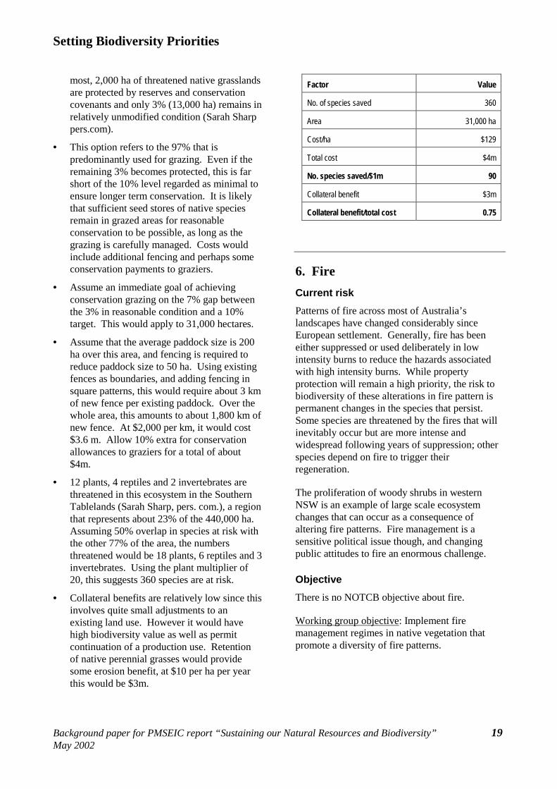
most, 2,000 ha of threatened native grasslands are protected by reserves and conservation covenants and only 3% (13,000 ha) remains in relatively unmodified condition (Sarah Sharp pers.com).

• This option refers to the 97% that is predominantly used for grazing. Even if the remaining 3% becomes protected, this is far short of the 10% level regarded as minimal to ensure longer term conservation. It is likely that sufficient seed stores of native species remain in grazed areas for reasonable conservation to be possible, as long as the grazing is carefully managed. Costs would include additional fencing and perhaps some conservation payments to graziers.

• Assume an immediate goal of achieving conservation grazing on the 7% gap between the 3% in reasonable condition and a 10% target. This would apply to 31,000 hectares.

• Assume that the average paddock size is 200 ha over this area, and fencing is required to reduce paddock size to 50 ha. Using existing fences as boundaries, and adding fencing in square patterns, this would require about 3 km of new fence per existing paddock. Over the whole area, this amounts to about 1,800 km of new fence. At $2,000 per km, it would cost $3.6 m. Allow 10% extra for conservation allowances to graziers for a total of about $4m.

• 12 plants, 4 reptiles and 2 invertebrates are threatened in this ecosystem in the Southern Tablelands (Sarah Sharp, pers. com.), a region that represents about 23% of the 440,000 ha. Assuming 50% overlap in species at risk with the other 77% of the area, the numbers threatened would be 18 plants, 6 reptiles and 3 invertebrates. Using the plant multiplier of 20, this suggests 360 species are at risk.

• Collateral benefits are relatively low since this involves quite small adjustments to an existing land use. However it would have high biodiversity value as well as permit continuation of a production use. Retention of native perennial grasses would provide some erosion benefit, at $10 per ha per year this would be $3m.

Factor Value


Area 31,000 ha

Cost/ha $129

Total cost $4m




6. Fire Current risk Patterns of fire across most of Australia’s landscapes have changed considerably since European settlement. Generally, fire has been either suppressed or used deliberately in low intensity burns to reduce the hazards associated with high intensity burns. While property protection will remain a high priority, the risk to biodiversity of these alterations in fire pattern is permanent changes in the species that persist. Some species are threatened by the fires that will inevitably occur but are more intense and widespread following years of suppression; other species depend on fire to trigger their regeneration.

The proliferation of woody shrubs in western NSW is an example of large scale ecosystem changes that can occur as a consequence of altering fire patterns. Fire management is a sensitive political issue though, and changing public attitudes to fire an enormous challenge.

Objective There is no NOTCB objective about fire.

Working group objective: Implement fire management regimes in native vegetation that promote a diversity of fire patterns.



Some management options R. Implement fire management regimes in native

vegetation which promote a diversity of fire patterns

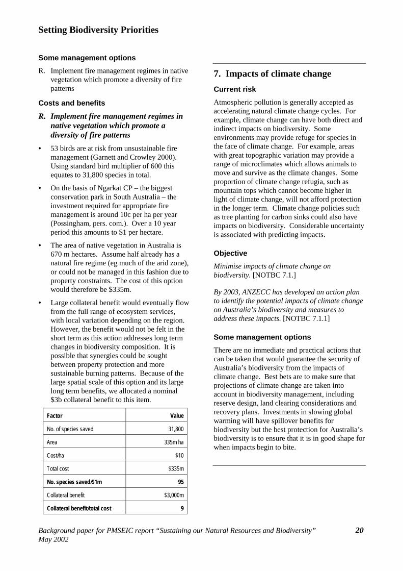
Costs and benefits R. Implement fire management regimes in

native vegetation which promote a diversity of fire patterns

• 53 birds are at risk from unsustainable fire management (Garnett and Crowley 2000). Using standard bird multiplier of 600 this equates to 31,800 species in total.

• On the basis of Ngarkat CP – the biggest conservation park in South Australia – the investment required for appropriate fire management is around 10c per ha per year (Possingham, pers. com.). Over a 10 year period this amounts to $1 per hectare.

• The area of native vegetation in Australia is 670 m hectares. Assume half already has a natural fire regime (eg much of the arid zone), or could not be managed in this fashion due to property constraints. The cost of this option would therefore be $335m.

• Large collateral benefit would eventually flow from the full range of ecosystem services, with local variation depending on the region. However, the benefit would not be felt in the short term as this action addresses long term changes in biodiversity composition. It is possible that synergies could be sought between property protection and more sustainable burning patterns. Because of the large spatial scale of this option and its large long term benefits, we allocated a nominal $3b collateral benefit to this item.

Factor Value


Area 335m ha

Cost/ha $10

Total cost $335m




7. Impacts of climate change Current risk Atmospheric pollution is generally accepted as accelerating natural climate change cycles. For example, climate change can have both direct and indirect impacts on biodiversity. Some environments may provide refuge for species in the face of climate change. For example, areas with great topographic variation may provide a range of microclimates which allows animals to move and survive as the climate changes. Some proportion of climate change refugia, such as mountain tops which cannot become higher in light of climate change, will not afford protection in the longer term. Climate change policies such as tree planting for carbon sinks could also have impacts on biodiversity. Considerable uncertainty is associated with predicting impacts.

Objective Minimise impacts of climate change on biodiversity. [NOTBC 7.1.]

By 2003, ANZECC has developed an action plan to identify the potential impacts of climate change on Australia’s biodiversity and measures to address these impacts. [NOTBC 7.1.1]

Some management options There are no immediate and practical actions that can be taken that would guarantee the security of Australia’s biodiversity from the impacts of climate change. Best bets are to make sure that projections of climate change are taken into account in biodiversity management, including reserve design, land clearing considerations and recovery plans. Investments in slowing global warming will have spillover benefits for biodiversity but the best protection for Australia’s biodiversity is to ensure that it is in good shape for when impacts begin to bite.



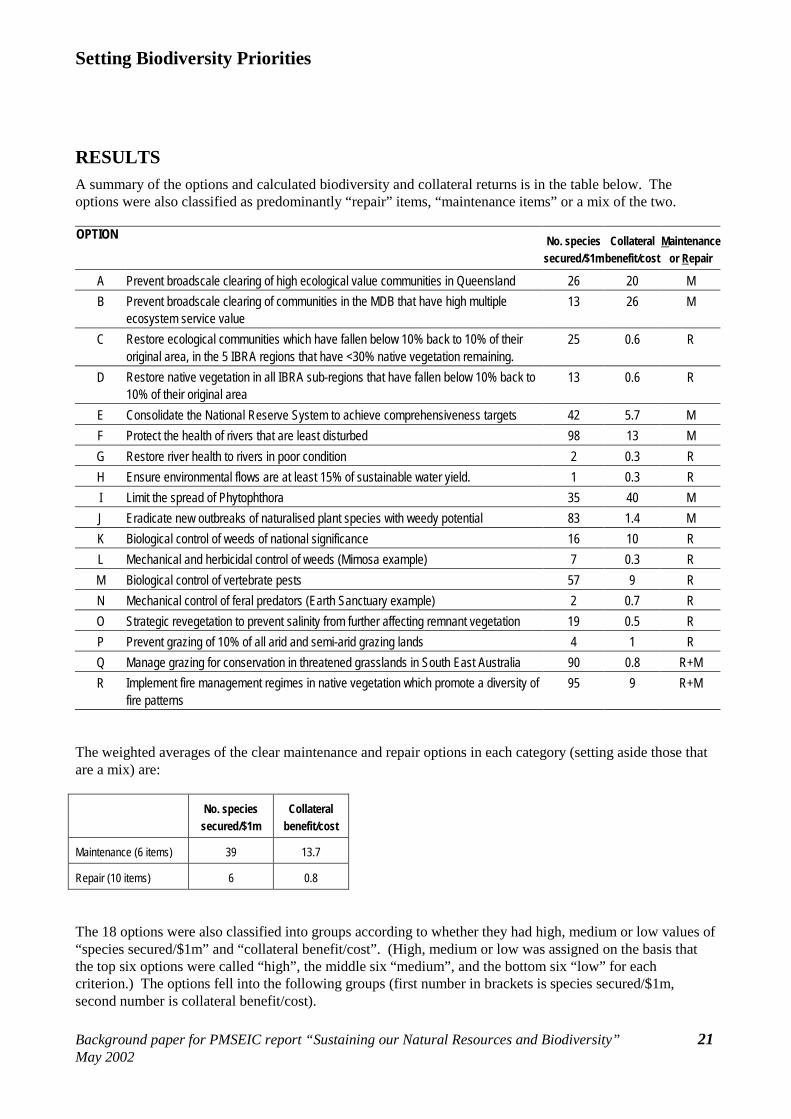
RESULTS A summary of the options and calculated biodiversity and collateral returns is in the table below. The options were also classified as predominantly “repair” items, “maintenance items” or a mix of the two.

OPTION No. species secured/$1m

Collateral benefit/cost

Maintenanceor Repair

A Prevent broadscale clearing of high ecological value communities in Queensland 26 20 M B Prevent broadscale clearing of communities in the MDB that have high multiple

ecosystem service value 13 26 M

C Restore ecological communities which have fallen below 10% back to 10% of their original area, in the 5 IBRA regions that have <30% native vegetation remaining.

25 0.6 R

D Restore native vegetation in all IBRA sub-regions that have fallen below 10% back to 10% of their original area

13 0.6 R

E Consolidate the National Reserve System to achieve comprehensiveness targets 42 5.7 M F Protect the health of rivers that are least disturbed 98 13 M G Restore river health to rivers in poor condition 2 0.3 R H Ensure environmental flows are at least 15% of sustainable water yield. 1 0.3 R I Limit the spread of Phytophthora 35 40 M J Eradicate new outbreaks of naturalised plant species with weedy potential 83 1.4 M K Biological control of weeds of national significance 16 10 R L Mechanical and herbicidal control of weeds (Mimosa example) 7 0.3 R M Biological control of vertebrate pests 57 9 R N Mechanical control of feral predators (Earth Sanctuary example) 2 0.7 R O Strategic revegetation to prevent salinity from further affecting remnant vegetation 19 0.5 R P Prevent grazing of 10% of all arid and semi-arid grazing lands 4 1 R Q Manage grazing for conservation in threatened grasslands in South East Australia 90 0.8 R+M R Implement fire management regimes in native vegetation which promote a diversity of

fire patterns 95 9 R+M

The weighted averages of the clear maintenance and repair options in each category (setting aside those that are a mix) are:

No. species secured/$1m

Collateral benefit/cost

Maintenance (6 items) 39 13.7

Repair (10 items) 6 0.8

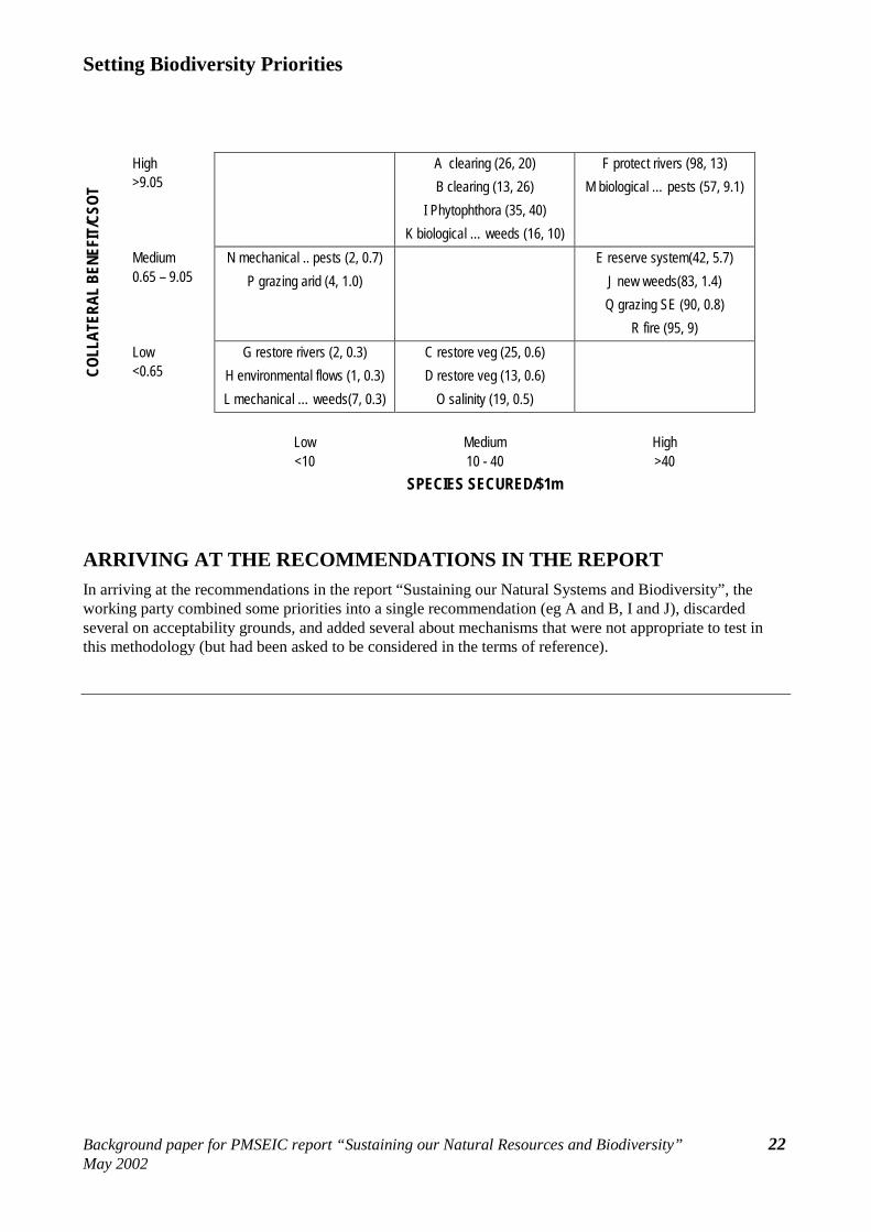
The 18 options were also classified into groups according to whether they had high, medium or low values of “species secured/$1m” and “collateral benefit/cost”. (High, medium or low was assigned on the basis that the top six options were called “high”, the middle six “medium”, and the bottom six “low” for each criterion.) The options fell into the following groups (first number in brackets is species secured/$1m, second number is collateral benefit/cost).



High >9.05

A clearing (26, 20) B clearing (13, 26)

I Phytophthora (35, 40) K biological … weeds (16, 10)

F protect rivers (98, 13) M biological … pests (57, 9.1)

Medium 0.65 – 9.05

N mechanical .. pests (2, 0.7) P grazing arid (4, 1.0)

E reserve system(42, 5.7) J new weeds(83, 1.4) Q grazing SE (90, 0.8)

R fire (95, 9)

COLL

ATER

AL B

ENEF

IT/C

SOT

Low <0.65

G restore rivers (2, 0.3) H environmental flows (1, 0.3) L mechanical … weeds(7, 0.3)

C restore veg (25, 0.6) D restore veg (13, 0.6)

O salinity (19, 0.5)

Low <10

Medium 10 - 40

High >40

SPECIES SECURED/$1m

ARRIVING AT THE RECOMMENDATIONS IN THE REPORT In arriving at the recommendations in the report “Sustaining our Natural Systems and Biodiversity”, the working party combined some priorities into a single recommendation (eg A and B, I and J), discarded several on acceptability grounds, and added several about mechanisms that were not appropriate to test in this methodology (but had been asked to be considered in the terms of reference).



References ACIL (1995) The economic impact of rabbits on

agricultural production in Australia: a preliminary assessment. Unpublished report, ACIL Economics and Policy, Canberra.

ANZECC (2001) Implications of salinity for biodiversity conservation and management. http://www.environment.sa.gov.au/biodiversity/pdfs/salinity_biodiversity.pdf

ARMCANZ and ANZECC (1999) The national weeds strategy: a strategic approach to weed problems of national significance. Commonwealth of Australia, Canberra.

Australian Science, Technology and Engineering Council (1996), Matching science and technology to future needs: 2010. www.isr.gov.au/science/astec/astec/future/final/futurea.html.

Australian Greenhouse Office (2001a) The Kyoto Protocol and greenhouse gas sinks. http://www.greenhouse.gov.au/pubs/factsheets/kyoto.pdf

Australian Greenhouse Office (2001b) National Greenhouse Gas Inventory 1999. http://www.greenhouse.gov.au/inventory/facts/01.html

Australian Greenhouse Office (2001c) Greenhouse Gas Abatement Program. http://www.greenhouse.gov.au/ggap/index.html

Ball, J (2001) Inland waters. Australia State of the Environment Report 2001 (Theme report). CSIRO Publishing on behalf of the Department of the Environment and Heritage, Canberra

Barson, M.M., Randall, L.A. and Bordas, V. (2000) Land cover change in Australia. Results of the collaborative Bureau of Rural Sciences – State Agencies’ project on Remote Sensing of Land Cover Change, Bureau of Rural Sciences, Canberra

Bureau of Tourism Research (2002) http://www.btr.gov.au/statistics/Datacard/datacard.html

Earth Sanctuaries (2001) Annual Report 2001. http://www.esl.com.au/2001/index.htm

Environment Australia (2001a) National Objectives and Targets for Biodiversity Conservation 2001-2005. Environment Australia, Canberra.

Environment Australia (2001b) A Directory of Australian Wetlands. Third edition. Environment Australia, Canberra.

Environment Australia (2001c) Threat abatement plan for dieback caused by the root-rot fungus Phytophthora cinnamomi. http://www.ea.gov.au/biodiversity/threatened/tap/phytophthora/index.html

Garnett S.T, and Crowley, G.M. (2000) The Action Plan for Australian Birds 2000. Environment Australia, Canberra.

Gibbs, D.M.H. and Muirhead, I.F. (1998) The economic value and environmental impact of the Australian beekeeping industry. http://honeybee.com.au/Library/gibsmuir.html

Gillespie, R. (2000) Economic values of the native vegetation of New South Wales. A background paper of the Native Vegetation Advisory Council of NSW. NSW Department of Land and Water Conservation.

Hardy, A.M. (2001) Terrestrial protected areas in Australia 2000: summary statistics from the Collaborative Protected Areas Database (CAPAD) 2001. Environment Australia, Canberra.

Morris (1996) Economic impact of RCD. Unpublished report for the Bureau of Resource Sciences by the Agricultural Economics Branch, Australian Bureau of Agricultural and Resource Economics, Canberra.

Murray Darling Basin Commission (1999) The salinity audit of the Murray Darling Basin. http://www.mdbc.gov.au/naturalresources/poli

http://www.isr.gov.au/science/astec/astec/future/final/futurea.html

http://www.isr.gov.au/science/astec/astec/future/final/futurea.html

http://www.greenhouse.gov.au/pubs/factsheets/kyoto.pdf

http://www.greenhouse.gov.au/pubs/factsheets/kyoto.pdf

http://www.greenhouse.gov.au/inventory/facts/01.html

http://www.greenhouse.gov.au/inventory/facts/01.html

http://www.greenhouse.gov.au/ggap/index.html

http://www.greenhouse.gov.au/ggap/index.html

http://www.btr.gov.au/statistics/Datacard/datacard.html

http://www.btr.gov.au/statistics/Datacard/datacard.html

http://www.esl.com.au/2001/index.htm

http://www.ea.gov.au/biodiversity/threatened/tap/phytophthora/index.html

http://www.ea.gov.au/biodiversity/threatened/tap/phytophthora/index.html

http://honeybee.com.au/Library/gibsmuir.html



cies_strategies/projectscreens/Salt_audit/salinity.htm

National Dryland Salinity Program (1998) Management Plan 1998-2003. http://www.ndsp.gov.au/15_publications/30_plans_and_strategies/05_mgt_plan/_the_challenge.html

National Land and Water Resources Audit (2000a) Landscape health in Australia. A rapid assessment of the relative condition of Australia’s bioregions and subregions. Environment Australia and National Land and Water Resources Audit, Canberra.

National Land and Water Resources Audit (2000b) Australian dryland salinity assessment 2000. Extent, impacts, processes, monitoring and management options. National Land and Water Resources Audit, Canberra

National Land and Water Resources Audit (2000c) Australian water resources assessment 2000. Surface water and groundwater – availability and quality. National Land and Water Audit, Canberra.

National Land and Water Resources Audit (2001) Australian native vegetation assessment 2001. National Land and Water Resources Audit, Canberra.

National Land and Water Resources Audit (2002) Australian catchment, river and estuary assessment 2002. National Land and Water Resources Audit, Canberra

Possingham, H.P. (2001) The business of biodiversity: Applying decision theory principles to nature conservation. Australian Conservation Foundation, Sydney

Schirmer, J. and Field, J. (2000) The cost of revegetation. Environment Australia, Canberra http://www.ea.gov.au/land/bushcare/publications/costrev/pubs/costrev.pdf

Thorp, J.R. and Lynch, R. (2000) The determination of weeds of national significance. National Weeds Strategy Executive Committee, Launceston.

Walpole, S., Sinden, J., and Yapp, T. (1996) Land quality as an input to production: the case of land degradation and agricultural output. Economic Analysis and Policy 26: 185-207.

Williams, J. et al. (2001) Biodiversity, Australia State of the Environment Report 2001 (Theme report). CSIRO Publishing on behalf of the Department of the Environment and Heritage, Canberra.

http://www.mdbc.gov.au/naturalresources/policies_strategies/projectscreens/Salt_audit/salinity.htm



http://www.ndsp.gov.au/15_publications/30_plans_and_strategies/05_mgt_plan/_the_challenge.html



http://www.ea.gov.au/land/bushcare/publications/costrev/pubs/costrev.pdf

http://www.ea.gov.au/land/bushcare/publications/costrev/pubs/costrev.pdf

setting setting biodiversity biodiversity prioritiespriorities · · 2013-06-20setting setting...

Documents