service time optimization of flow shop systems · service time optimization of flow shop systems a...
TRANSCRIPT
SERVICE TIME OPTIMIZATION OF FLOWSHOP SYSTEMS
a dissertation submitted to
the department of industrial engineering
and the institute of engineering and science
of bilkent university
in partial fulfillment of the requirements
for the degree of
doctor of philosophy
By
Ömer Selvi
November, 2008
I certify that I have read this thesis and that in my opinion it is fully adequate,
in scope and in quality, as a dissertation for the degree of doctor of philosophy.
Asst. Prof. Dr. Ka¼gan Gökbayrak (Supervisor)
I certify that I have read this thesis and that in my opinion it is fully adequate,
in scope and in quality, as a dissertation for the degree of doctor of philosophy.
Prof. Dr. M. Selim Aktürk
I certify that I have read this thesis and that in my opinion it is fully adequate,
in scope and in quality, as a dissertation for the degree of doctor of philosophy.
Prof. Dr. Erdal Erel
ii
I certify that I have read this thesis and that in my opinion it is fully adequate,
in scope and in quality, as a dissertation for the degree of doctor of philosophy.
Prof. Dr. Ömer K¬rca
I certify that I have read this thesis and that in my opinion it is fully adequate,
in scope and in quality, as a dissertation for the degree of doctor of philosophy.
Assoc. Prof. Dr. Emre Alper Y¬ld¬r¬m
Approved for the Institute of Engineering and Science:
Prof. Dr. Mehmet B. BarayDirector of the Institute
iii
ABSTRACT
SERVICE TIME OPTIMIZATION OF FLOW SHOPSYSTEMS
Ömer SelviPh.D. in Industrial Engineering
Supervisor: Asst. Prof. Dr. Ka¼gan GökbayrakNovember, 2008
One of the key questions that engineers face in �ow shop systems is the servicetime control, i.e., how long jobs should be processed at each machine. This is animportant question because processing times can have great impacts on the coste¢ ciency of the �ow shop systems. In order to meet job completion deadlines andto decrease inventory costs, one may set the service times as small as possible;however, this usually comes at the expense of reduced tool life increasing servicecosts. In this thesis, we study the �ow shop systems under such trade-o¤s. Weconsider the service time optimization of deterministic �ow shop systems process-ing identical jobs that arrive at the system at known times and are processed inthe order they arrive within deadlines. The cost function to be minimized con-sists of service costs at machines and regular completion-time costs of jobs. Thedecision variables are the service times that are controllable within constraints.
We �rst consider the �xed service time �ow shop systems formed of initiallycontrollable machines, where the service times are set only once at the startup time and cannot be altered between processes, and uncontrollable machines,where the service times are �xed and known in advance. For such systems, weformulate a non-convex and non-di¤erentiable optimization problem with a stan-dard solution procedure based on the linearization of the constraints allowing fora convex optimization problem with high memory requirements. Regardless ofthe cost function, we present a set of waiting and completion time characteristicsin such �ow shop systems and employ them to derive a simpler equivalent convexoptimization problem which improves solution times and alleviates the memoryrequirements enabling solutions for larger systems. However, the resulting sim-pli�ed convex optimization problem still needs the use of a convex optimizationsolver which may not be available at some of the manufacturing companies. To
iv
overcome such need, we introduce another equivalent convex optimization prob-lem along with its subgradient algorithm yielding substantial improvements insolution times and solvable system sizes. We also consider a speci�c nonlineardecreasing service cost structure allowing us to introduce a new search algorithmmuch faster than the subgradient solution algorithm.
Building on the results for �xed service time �ow shop systems, we also con-sider the mixed line �ow shop systems formed of fully controllable machines,where the service times are adjustable for each process, initially controllable ma-chines, and uncontrollable machines. Similarly, we formulate a non-convex andnon-di¤erentiable optimization problem for such systems and, as a standard wayof solving the formulated problem, we apply the method of linearization on theconstraints to present a convex optimization problem with high memory require-ments. Then, we present a set of optimal waiting characteristics in such �owshop systems and employ them to derive simpler equivalent convex optimizationproblems. A "forward in time" algorithm is also proposed to decompose theresulting simpli�ed equivalent convex optimization problem into smaller convexoptimization problems for the �ow shop systems formed of only fully control-lable and uncontrollable machines. The computational results demonstrate thatthe simpli�cations and the decomposition not only improve the solution timesconsiderably but also allow us to solve larger problems by alleviating memoryconstraints.
Keywords: Deterministic �ow shop systems, Optimal control, Controllable servicetimes, Controllable/Uncontrollable machines, Convex programming, Subgradientalgorithm.
v
ÖZET
AKIS T·IP·I ·ISL·IK S·ISTEMLERDE ·ISLEM SÜRELER·IEN·IY·ILEMES·I
Ömer SelviEndüstri Mühendisli¼gi, Doktora
Tez Yöneticisi: Asst. Prof. Dr. Ka¼gan GökbayrakKas¬m, 2008
Mühendislerin ak¬s tipi islik sistemlerde cevaplamas¬gereken en kilit sorulardanbirisi islem sürelerinin nas¬l denetlenece¼gidir yani islerin her makinede ne kadarsüre islem görmesi gerekti¼gidir. Bu önemli bir sorudur çünkü islem sürelerininak¬s tipi islik sistemlerin maliyet verimlili¼gi üzerinde çok büyük etkileri olabilir.·Isleri son bitim zaman¬na kadar tamamlamak ve envanter maliyetlerini düsürmekiçin islem süreleri mümkün oldu¼gunca küçük tutulabilir, fakat bu yaklas¬m genel-likle islemmaliyetlerini yükselten k¬salt¬lm¬s tak¬m ömürlerinden do¼gan masra�ar¬beraberinde getirir. Biz bu tezde ak¬s tipi islik sistemlerde bu tip iliskiler üzer-ine çal¬st¬k. Bilinen zamanlarda gelen isleri geldikleri s¬rayla isleyen belirlen-imci ak¬s tipi islik sistemlerde islem süreleri eniyilemesi problemini ele ald¬k.Enküçültülecek maliyet fonksiyonunu makinelerdeki islem maliyetlerinden ve ku-rall¬is bitim zaman¬maliyetlerinden olusturduk. Bir k¬s¬t dahilinde denetlenebilirislem sürelerini karar de¼giskenleri olarak belirledik.
Öncelikle, baslang¬çta denetlenebilir, yani islem süreleri sistemin çal¬smayabaslama an¬nda belirlenen ve islemler aras¬nda bir daha de¼gistirilemeyen, vedenetlenemez, yani islem süreleri sabit olan ve önceden bilinen, makinelerdenolusan sabit islem süreli ak¬s tipi islik sistemleri ele ald¬k. Bu tip sistemler içinstandart çözüm yöntemi yüksek bellek gereksinimli bir d¬sbükey eniyileme prob-lemine olanak sa¼glayan k¬s¬tlar¬n do¼grusallast¬r¬lmas¬metoduna dayanan d¬sbükeyolmayan ve türevlenemeyen bir eniyileme problemi olusturduk. Maliyet fonksiy-onundan ba¼g¬ms¬z olarak, bu tip ak¬s tipi islik sistemler için bir dizi bekleme veis bitim zaman¬özellikleri gösterdik ve bu özellikleri kullanarak çözüm sürelerinigelistiren ve daha büyük sistemlerin çözülmesine olanak sa¼glayacak sekilde bellekgereksinimini azaltan daha basit ve denk bir d¬sbükey eniyileme problemi ç¬kard¬k.Ne var ki sonuçta ortaya ç¬kan basitlestirilmis d¬sbükey eniyileme problemi hala
vi
baz¬ imalatç¬ sirketlerin tedarik edemeyece¼gi d¬sbükey eniyileme çözücüsü kul-lan¬m¬na ihtiyaç duymaktad¬r. Bu ihtiyac¬gidermek için çözüm sürelerinde veçözülebilir sistem boyutlar¬nda oldukça ciddi iyilestirme sa¼glayan altgradyan al-goritmas¬esli¼ginde bir baska denk d¬sbükey eniyileme problemi önerdik. Ayr¬ca,altgradyan algoritmas¬ndan çok daha h¬zl¬ çal¬san yeni bir tarama algoritmas¬gelistirmemize olanak sa¼glayan do¼grusal olmayan ve azalan özel bir islem maliyetyap¬s¬n¬da çözümledik.
Sabit islem süreli ak¬s tipi islik sistemler için geçerli sonuçlar¬n üzerine insaetmek suretiyle, bu tezde ayr¬ca tamamen denetlenebilir, yani islem süreleriher islem için ayr¬ ayr¬ ayarlanabilen, baslang¬çta denetlenebilir ve denetlene-mez makinelerden olusan ak¬s tipi islik sistemleri de ele ald¬k. Benzer sekilde,bu tip sistemler için d¬sbükey olmayan ve türevlenemeyen bir eniyileme prob-lemi olusturduk ve olusturdu¼gumuz bu probleme standart çözüm yöntemi olarak,k¬s¬t do¼grusallast¬rma metodu uygulamak suretiyle yüksek bellek gereksinimli bird¬sbükey eniyileme problemi ortaya koyduk. Daha sonra, bu tip ak¬s tipi islik sis-temler için bir dizi en iyi bekleme özellikleri gösterdik ve bu özellikleri kullanarakdaha basit ve denk bir d¬sbükey eniyileme problemi ç¬kard¬k. Sadece tamamendenetlenebilir ve denetlenemez makinelerden olusan ak¬s tipi islik sistemler için,sonuçta ortaya ç¬kan basitlestirilmis d¬sbükey eniyileme problemini daha küçükd¬sbükey eniyileme problemlerine ayr¬st¬ran "zamanda ilerleyen" bir algoritmada önerdik. Deneysel hesaplamalar¬m¬z gösterdi ki basitlestirmeler ve ayr¬st¬rmasadece çözüm sürelerini gelistirmekle kalmad¬ayn¬zamanda bellek gereksiniminiazaltmak suretiyle daha büyük sistemleri çözmemize olanak sa¼glad¬.
Anahtar sözcükler : Belirlenimci ak¬s tipi islik sistemler, En iyi denetleme,Denetlenebilir islem süreleri, Denetlenebilir/denetlenemez makineler, D¬sbükeyprogramlama, Altgradyan algoritmas¬.
vii
Dedicated
to
my family
viii

Acknowledgement
I would like to sincerely thank my advisor Asst. Prof. Dr. Ka¼gan Gökbayrak
for his valuable and perpetual guidance and encouragement throughout this study.
His supervising with patience and interest made this thesis possible.
I gratefully acknowledge all the members of my committee who have given
their time to read this manuscript and o¤ered valuable advice.
My special thanks go to my family for their encouragement and sacri�ce. This
study is dedicated to them without whom it would not have been possible.
ix
Contents
1 Introduction 1
2 Fixed Service Time Flow Shop Systems 9
2.1 Problem Formulation . . . . . . . . . . . . . . . . . . . . . . . . . 11
2.2 Waiting Characteristics of Fixed Service Time Flow Shop Systems 15
2.3 Simpli�ed Convex Optimization Problem . . . . . . . . . . . . . . 26
2.4 Subgradient Descent Algorithm with Projections . . . . . . . . . . 27
2.5 Two-Phase Search Algorithm . . . . . . . . . . . . . . . . . . . . 32
2.5.1 Determining the Minimizers of fJkgNk=1 Functions . . . . . 35
2.5.2 Locating the Optimal Solution of JR . . . . . . . . . . . . 41
2.5.3 The Algorithm . . . . . . . . . . . . . . . . . . . . . . . . 48
2.6 Numerical Study . . . . . . . . . . . . . . . . . . . . . . . . . . . 50
2.6.1 Veri�cation of the Waiting Characteristics . . . . . . . . . 50
2.6.2 Comparison of Di¤erent Solution Methodologies . . . . . . 52
2.7 Conclusion . . . . . . . . . . . . . . . . . . . . . . . . . . . . . . . 56
x
3 Mixed Line Flow Shop Systems 58
3.1 Problem Formulation . . . . . . . . . . . . . . . . . . . . . . . . . 60
3.2 Waiting Characteristics of the Optimal Sample Path . . . . . . . 64
3.2.1 Initially Controllable Portions . . . . . . . . . . . . . . . . 64
3.2.2 Fully Controllable Portions . . . . . . . . . . . . . . . . . . 72
3.3 Simpli�ed Convex Optimization Problems . . . . . . . . . . . . . 83
3.3.1 Flow Shop Systems Starting with Fully Controllable Portions 83
3.3.2 Flow Shop Systems Starting with Initially Controllable Por-
tions . . . . . . . . . . . . . . . . . . . . . . . . . . . . . . 85
3.4 Forward Decomposition Algorithm . . . . . . . . . . . . . . . . . 88
3.5 Numerical Study . . . . . . . . . . . . . . . . . . . . . . . . . . . 100
3.5.1 Veri�cation of the Optimal Waiting Characteristics . . . . 101
3.5.2 Analysis of the Replacement of Initially Controllable Ma-
chines with Fully Controllable Machines . . . . . . . . . . 103
3.5.3 Analysis of the E¤ects of the Locations of Fully Control-
lable Machines . . . . . . . . . . . . . . . . . . . . . . . . 104
3.5.4 Analysis of the Relative E¤ects of Service and Completion-
Time Costs on the Optimal Solution . . . . . . . . . . . . 106
3.5.5 Comparison of Di¤erent Solution Methodologies . . . . . . 107
3.6 Conclusion . . . . . . . . . . . . . . . . . . . . . . . . . . . . . . . 111
4 Conclusion 113
4.1 Concluding Remarks . . . . . . . . . . . . . . . . . . . . . . . . . 113
xi
4.2 Model Extensions . . . . . . . . . . . . . . . . . . . . . . . . . . . 117
4.3 Future Research Directions . . . . . . . . . . . . . . . . . . . . . . 118
xii
List of Figures
2.1 Flowchart of the Two-Phase Search Algorithm . . . . . . . . . . . 49
2.2 Evolutions of Service Times for Subgradient Descent Algorithm . 53
3.1 Optimal Service Times Averaged over All Jobs at Machines versus
Weight of Total Service Cost . . . . . . . . . . . . . . . . . . . . . 107
3.2 Optimal Service Times Averaged over All Jobs at Machines versus
�2 value at Machine 2 . . . . . . . . . . . . . . . . . . . . . . . . 108
xiii
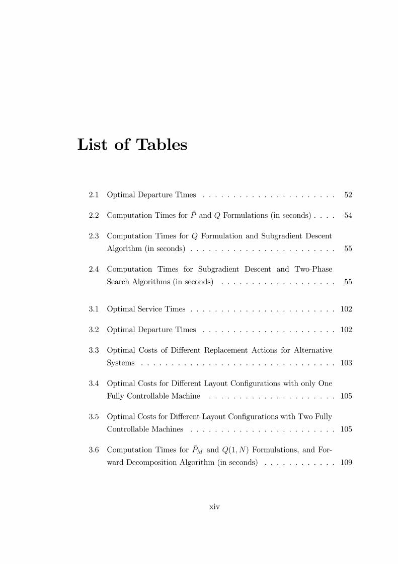
List of Tables
2.1 Optimal Departure Times . . . . . . . . . . . . . . . . . . . . . . 52
2.2 Computation Times for �P and Q Formulations (in seconds) . . . . 54
2.3 Computation Times for Q Formulation and Subgradient Descent
Algorithm (in seconds) . . . . . . . . . . . . . . . . . . . . . . . . 55
2.4 Computation Times for Subgradient Descent and Two-Phase
Search Algorithms (in seconds) . . . . . . . . . . . . . . . . . . . 55
3.1 Optimal Service Times . . . . . . . . . . . . . . . . . . . . . . . . 102
3.2 Optimal Departure Times . . . . . . . . . . . . . . . . . . . . . . 102
3.3 Optimal Costs of Di¤erent Replacement Actions for Alternative
Systems . . . . . . . . . . . . . . . . . . . . . . . . . . . . . . . . 103
3.4 Optimal Costs for Di¤erent Layout Con�gurations with only One
Fully Controllable Machine . . . . . . . . . . . . . . . . . . . . . 105
3.5 Optimal Costs for Di¤erent Layout Con�gurations with Two Fully
Controllable Machines . . . . . . . . . . . . . . . . . . . . . . . . 105
3.6 Computation Times for �PM and Q(1; N) Formulations, and For-
ward Decomposition Algorithm (in seconds) . . . . . . . . . . . . 109
xiv
3.7 Computation Times for Virtual Deadline Algorithm and Forward
Decomposition Algorithm (in seconds) . . . . . . . . . . . . . . . 111
xv
Chapter 1
Introduction
Flow shop systems have been an important area of research ever since 1950�s.
Since �ow shop systems can often be found throughout many industries, i.e.,
manufacturing (e.g. automobile) industry, many researchers have recognized the
importance of the subject and contributed to it. One of the key questions that
engineers face in �ow shop systems is the service time control, i.e., how long jobs
should be processed at each machine. This is an important question because
service times can have great impacts on the cost e¢ ciency of �ow shop systems.
Taylor�s tool wear equation [24] states that tool life decreases rapidly with an
increase in machining speed. Increased machining speeds may also result in more
frequent tool breakages. Hence, increasing machining speeds rapidly increases
the frequency of tool changing which implies increased tooling costs. Moreover,
tooling has also direct cost implications. Industry data suggests that tooling, as
one of the major component, accounts for 25% to 30% of production cost in an
automated machining environment (see [26]). In �exible manufacturing systems
(FMSs), the initial investment in cutting tools and �xtures may reach up to 25%
of the total FMS investment (see [46]). Seven to ten times more money is spent
on tools, jigs, �xtures, and consumables than on capital equipment during the
useful life of the machines (see [3]). The impact of tooling problems on system
management should also not be underestimated: 40% to 60% of a foreman�s time
is spent expediting tools and materials, 15% to 20% of scheduled production time
1
CHAPTER 1. INTRODUCTION 2
is missed due to unavailable tooling.
It is evident from the above discussion that, to decrease tooling costs, it is
preferred to decrease machining speeds and, therefore, to increase service times
as much as possible. However, longer service times mean longer �ow times (time
required to move a job through the system, from entry on the �rst machine to
completion on the last machine) of jobs. Increased �ow times require the antici-
pation of customers�needs in terms of product variations, options, and extra �n-
ished goods as well as work-in-process (WIP) inventories due to longer deliveries.
Capital invested to inventories as long as they remain in the system provides no
pro�t. Inventory quality also decreases as the un�nished items spend more time
in the system because they are vulnerable to damages. Moreover, the ability to
adapt the production structure according to the fast changing global market and
to respond customer needs relies on shorter �ow times and lower work-in-process
inventories. For instance, a manufacturing system with shorter �ow times elim-
inates the necessity of further �nished products and WIP inventories, provides
greater freedom of choice to the customer, and, therefore, becomes more com-
petitive against any alternative system with longer delivery times. Many other
advantages such as correcting quality problems and implementing engineering
changes accompany to these due to faster responsiveness. Hence, to decrease
the cost related to inventory held and customer satisfaction, which is hard to be
quanti�ed, service times are tried to be reduced as much as possible.
In this thesis, we study the �ow shop systems under such trade-o¤s. We con-
sider the service time optimization of deterministic �ow shop systems processing
identical jobs that arrive at the system at known times and are processed within
their associated deadlines. The term "identical" used for jobs implies that the
operational requirements of all jobs so as to change their physical characteristics
according to certain speci�cations are the same at each machine so that each
machine has its own speci�c service cost function applied to all jobs processed,
i.e., homogeneous (same for each job but not for each machine) service cost func-
tions are employed for jobs at machines. The �ow shop system that we consider
consists of fully controllable machines, where the service times are adjustable be-
fore each process, initially controllable machines, where the service times are set
CHAPTER 1. INTRODUCTION 3
only once at the start up time and could not be altered between processes, and
uncontrollable machines, where the service times are �xed and known a priori.
The existing CNC (Computer Numerical Control) machine technology allows us
to change the service times very quickly by just changing few lines in the CNC
programming code without incurring setup times and production errors. Hence,
CNC machines are good examples of fully controllable machines. As opposed to
CNC machines, some traditional (non-CNC) machines are manually controlled
by human operators. During mass production, it may not be feasible to alter
the service times of these machines because the setup times are idle times and
the manual modi�cations are prone to errors. Therefore, the service times at
these traditional machines are uncontrollable or initially controllable, i.e., they
are set at the start-up time and are not altered afterwards. The cost objective
we consider consists of service costs at fully and initially controllable machines,
which are dependent on service times, and regular completion-time costs for jobs.
Motivated by the above discussion, we assume that faster services increase service
costs. Slower services, on the other hand, increase the regular completion-time
costs and/or leading to the violation of constraints on job completion deadlines.
This trade-o¤ in setting the service times makes the problem nontrivial and we
set our objective to determine the cost-minimizing service times.
The scheduling problems of the �ow shops are known to be NP-hard even
for �xed service times (see [39]). In these problems, the objective is to �nd
the best sequence of jobs to be processed at machines. Except for two-machine
systems with the objective of minimizing makespan, the scheduling literature for
the �ow shop systems is limited to heuristics and approximate solution methods.
Introduction of controllable service times at machines further complicates the
problem. A survey of results on the controllable service times in scheduling
problems can be found in [36], [19], and [44]. In this thesis, searching for e¢ cient
solution methodologies yielding true optimal solutions, we assume that jobs are
processed in the order they arrive at machines, i.e., the machines operate on a
non-preemptive �rst-come �rst-served policy.
The related optimal control literature, on the other hand, assumed that jobs
are processed in a given sequence, and concentrated on determining the optimal
CHAPTER 1. INTRODUCTION 4
control inputs which in turn determine the optimal service times. The idea of
treating scheduling problems for deterministic queues as optimal control problems
on discrete event dynamic systems �rst appeared in [12] where job arrival times
to a single machine system were controlled to minimize the discrepancy between
job completion times and desired due dates. Following this work, service time
control problems for the systems, where the job arrival times are known in ad-
vance and the service times can be adjusted between processes, were considered.
Pepyne and Cassandras, in [37], formulated a non-convex and non-di¤erentiable
optimal control problem for a single machine system with the objective of com-
pleting jobs as fast as possible with the least amount of control e¤ort and used
calculus of variations techniques to obtain structural properties of the optimal
solution. In [38], Pepyne and Cassandras extended their results to jobs with non-
regular completion-time costs penalizing earliness and tardiness with given due
dates. The task of solving these problems was simpli�ed by exploiting structural
properties of the optimal sample path and it was shown that the optimal solution
is unique by Cassandras et al. [7]. Further exploiting the structural properties
of the optimal sample path for the single machine problem, �backward in time�
and "forward in time" algorithms based on the decomposition of the original non-
convex and non-di¤erentiable optimization problem into a set of smaller convex
optimization problems with linear constraints were presented by Wardi et al. [47]
and Cho et al. [10], respectively. The "forward in time" algorithm presented by
Cho et al. [10] was later improved by Zhang and Cassandras [48]. In a related
work, Cassandras and Mookherjee [6] studied the case of uncertainty where only
some future arrival information is available within a time window of length T and
introduced a receding horizon control scheme along with its several properties en-
abling the use of a controller based on rough estimates of unknown future arrivals
with limited loss of optimality properties. Moon and Wardi [34] considered a sin-
gle machine problem where the completed jobs wait in a �nite size output bu¤er
until their due dates. They presented an e¢ cient solution algorithm for this
system with blocking. Mao et al. [32] removed the completion-time costs and
introduced deadline constraints. Some optimal solution properties of the result-
ing problem were identi�ed leading to a highly e¢ cient solution algorithm under
the assumption that a feasible solution exists. In the absence of feasible solutions
CHAPTER 1. INTRODUCTION 5
due to deadline constraints, Mao and Cassandras [29] introduced an admission
control scheme in which some jobs are removed with the objective of maximizing
the number of remaining jobs which are all guaranteed feasibility and, through
derivation of several optimality properties, developed a computationally e¢ cient
algorithm for solving the resulting admission control problem.
Flow shop systems are not the simple extensions of the single machine sys-
tems. It is much more di¢ cult to solve the service time optimization problems
in �ow shop systems for two main reasons: i) there is an M -fold (where M � 2is the number of machines in the �ow shop) increase in the dimensionality of the
decision variables, and ii) coupling among the machines�dynamics causes the fail-
ure of the structural properties exploited in single machine systems. Due to these
di¢ culties, only a few works were conducted on the service time optimization
problems on �ow shop systems in the optimal control literature. The work on
service time control problems for �ow shop systems with identical jobs started out
with Cassandras et al. [5], which derived some necessary conditions for optimality
and introduced a solution technique using the Bezier approximation method for
a two-machine �ow shop system. Recently, building on the works in [32], Mao
and Cassandras [30] considered two-machine �ow shop systems with service costs
that are decreasing on service times and derived some optimality properties that
led to an iterative algorithm, which was shown to converge. The results in [30],
were later extended to multi-machine �ow shop systems with nonidentical jobs
by Mao and Cassandras [31]. To the best of our knowledge, Mao and Cassandras
[31] is the only study on service time optimization of multi-machine �ow shop
systems in the optimal control literature. Therefore, we can say that service time
optimization of �ow shops needs further attention and we aim to contribute to
the literature in that sense.
In this thesis, we consider the �ow shop system in Mao and Cassandras [31]
with identical jobs and introduce initially controllable and uncontrollable ma-
chines, and job completion-time costs. Although it seems to be a simple extension,
structural properties allowing for an e¢ cient solution procedure for the system
in [31], which focuses only on service costs at machines, no longer hold when we
include job completion-time costs in the objective function even in the absence
CHAPTER 1. INTRODUCTION 6
of initially controllable and uncontrollable machines. Hence, the analysis changes
completely. We �rst formulate an optimization problem minimizing a convex
cost objective over a non-convex feasible region due to max-plus algebra used
for the representation of departures of jobs from machines, which is, therefore,
non-convex and non-di¤erentiable. The standard way of solving this non-convex
and non-di¤erentiable problem is indeed to apply linearization on the equality
constraints including max function to convexify the feasible region. However,
the linearization process, which replaces each max equality constraint with two
inequality constraints, doubles the number of constraints in the resulting convex
formulation. Hence, the numeric solution of this convex optimization problem
demands a large memory limiting the solvable system sizes due to its increased
dimensionality. Hence, we search for more e¢ cient solution methodologies in
terms of both solvable system sizes and solution times in this thesis.
In Chapter 2, we consider the �ow shop systems consisting only of initially
controllable and uncontrollable machines termed �xed service time �ow shop sys-
tems. In order to relieve the memory bottleneck for the convex formulation
derived through aforementioned linearization process, we present a set of wait-
ing and completion time characteristics of �xed service time �ow shop systems
regardless of the cost objective. Mainly, we show that no waiting is observed
after the slowest machine, i.e., machine with the highest service time, of the sys-
tem and jobs that do not wait at the slowest machine observe no waiting in the
system. Based on these results, we introduce two alternative representations for
the job completion times. Employing the �rst representation, we derive a simpli-
�ed equivalent convex optimization problem, which improves the solution times
and enables solutions for larger systems due to less memory requirements than
the convex optimization problem obtained through linearization. However, the
resulting simpli�ed convex optimization problem still needs the use of a convex
optimization solver which may not be available at some of the manufacturing
companies. Hence, motivated by the need for a lower cost optimization tool, we
employ the second representation of job completion times to introduce another
equivalent convex optimization problem, which is non-di¤erentiable, along with
its subgradient descent algorithm. As demonstrated by a numerical study, the
CHAPTER 1. INTRODUCTION 7
subgradient descent algorithm not only eliminates the need for convex optimiza-
tion solvers but also allows for the solution of larger systems due to its much less
memory requirements and improves the solution times signi�cantly. We also an-
alyze a speci�c service cost structure inversely proportional to the services times.
This cost structure allows us to sort the optimal service times of the machines and
to introduce a new search algorithm much faster than the subgradient descent
solution algorithm.
In Chapter 3, building on the results for �xed service time �ow shop sys-
tems, we consider the �ow shop systems formed of fully controllable, initially
controllable and uncontrollable machines termed mixed line �ow shop systems.
Existence of fully controllable machines in the system brings new structural prop-
erties leading to new solution methodologies di¤erent from the ones developed for
�xed service time �op shop systems. Hence, we continue with a new chapter for
mixed line �ow shops systems. To overcome the problem of limitation on solvable
system sizes due to the huge memory requirements of the resulting convex opti-
mization problem obtained through linearization on the max constraints, and to
improve the solution times, we �rst present a set of optimal waiting character-
istics of these systems. In particular, under the strict convexity assumption of
service costs, we show that jobs do not wait on the optimal sample path after
the �rst fully controllable machine. Employing the no-wait property, we then
derive simpli�ed equivalent convex optimization problems. For the �ow shop
systems formed of only fully controllable and uncontrollable machines, the asso-
ciated simpli�ed equivalent convex optimization problem is then decomposed by
a "forward in time" algorithm into smaller convex optimization problems under
an additional strict convexity assumption on the job completion-time costs. As
shown by a computational study, the simpli�cations and the decomposition not
only improve the solution times considerably but also allow us to solve larger
problems by alleviating memory constraints.
The rest of the thesis is organized as follows: In Chapter 2, we formulate a
non-convex and non-di¤erentiable optimization problem for the �ow shop sys-
tems formed of initially controllable and uncontrollable machines and obtain a
convex programming formulation by the standard method of linearization. A set
CHAPTER 1. INTRODUCTION 8
of waiting and completion time characteristics of these systems regardless of the
objective function is derived. These characteristics are then employed to derive
a simpler equivalent convex optimization problem and another alternative equiv-
alent convex optimization problem along with a subgradient descent algorithm.
Finally, a new search algorithm is developed for a speci�c nonlinear decreasing
service cost structure in this chapter. In Chapter 3, we formulate a non-convex
and non-di¤erentiable optimization problem for the �ow shop systems formed
of fully controllable, initially controllable, and uncontrollable machines and ob-
tain a convex programming formulation by the standard method of linearization.
We derive a set of optimal waiting characteristics of such systems and exploit
them to derive equivalent simpli�ed convex optimization problems. A forward
decomposition algorithm is also presented in this chapter to decompose the asso-
ciated simpli�ed convex optimization problem into smaller convex optimization
problems with linear constraints. Finally, we give concluding remarks, model
extensions, and future research directions in Chapter 4.
Chapter 2
Service Time Optimization of
Fixed Service Time Flow Shop
Systems
In this chapter, we consider deterministic �ow shop systems formed only of ini-
tially controllable and uncontrollable machines processing identical jobs with
known arrival times and deadlines. Since the service times are �xed at the start-
up time and are not changed during the whole process, we de�ne these systems
as �xed service time �ow shops. The cost function we consider consists of service
costs at initially controllable machines and regular completion-time costs of jobs.
Motivated by the extended Taylor�s tool-wear equation [24], we assume that faster
services increase wear and tear on the tools due to increased temperatures, and
may raise the need for extra supervision, increasing service costs. The losses of
the product quality due to faster services are also lumped into these service costs.
Slower services, on the other hand, may delay the completion times increasing
the completion-time costs and/or leading to untimely job completions. We ac-
knowledge this trade-o¤and set our objective as to determine the cost-minimizing
service times.
In this chapter, we formulate a non-convex and non-di¤erentiable optimization
9
CHAPTER 2. FIXED SERVICE TIME FLOW SHOP SYSTEMS 10
problem and apply the standard method of linearization on the max constraints
to get a convex formulation. Since, the resulting convex formulation provides
solution only for small systems due to its high memory requirements, aiming to
solve larger systems and to improve solution times, we �rst derive a set of waiting
and completion time characteristics for such systems independent of the cost ob-
jective. Basically, we show that no waiting is observed at the downstream of the
machine with the highest service time and if a job does not wait at this machine,
it also observes no waiting in the system. Then, we exploit these waiting charac-
teristics to derive an alternative representation of job completion times allowing
us to present a simpler equivalent convex optimization problem. However, even
though the resulting convex problem formulation improves the solution times and
enables solutions for larger systems, it still needs the use of a solver which may
not be available at some manufacturing companies. Hence, further exploiting the
waiting and completion time characteristics, we come up with another alterna-
tive representation of job completion times and employ it to introduce another
equivalent convex optimization problem, which is non-di¤erentiable. A subgra-
dient descent algorithm is also developed for solving this optimization problem.
This algorithm eliminates the need for a solver and has considerably low memory
requirements; therefore, it allows us to solve optimization problems of even larger
systems in much shorter times. We also analyze a special case where the ser-
vice costs at machines are nonlinear decreasing functions of service times. This
cost structure allows us to sort the optimal service times of machines. First,
we de�ne di¤erentiable subproblems that can be solved easily. Employing these
subproblems, we then introduce a two-phase search algorithm that converges in
a �nite number of steps. Through improving the solution times drastically, this
new search algorithm eliminates the need for the subgradient descent solution
algorithm whose performance, as a drawback, is highly a¤ected by the selection
of its termination tolerance and step sizes at each iteration.
The rest of the chapter is organized as follows: We formulate a non-convex and
non-di¤erentiable optimization problem and apply the linearization method yield-
ing a convex optimization problem in Section 2.1. In Section 2.2, regardless of the
objective function, we derive a set of waiting and completion time characteristics
CHAPTER 2. FIXED SERVICE TIME FLOW SHOP SYSTEMS 11
for �xed service time �ow shop systems. Employing the waiting and completion
time characteristics in �xed service time �ow shop systems derived in Section 2.2,
a simpler equivalent convex optimization problem is introduced in Section 2.3. In
Section 2.4, an alternative equivalent convex optimization problem is presented
along with a subgradient descent algorithm with projections. For a special type
service cost structure inversely proportional to the service times, we de�ne dif-
ferentiable subproblems and present a two-phase search algorithm in Section 2.5.
Section 2.6 presents a numerical example to illustrate the waiting and comple-
tion time characteristics derived in Section 2.2 under optimal service times. In
this section, we also compare the performances of the proposed methodologies in
terms of the solution times and the solvable system sizes through a computational
study. Finally, Section 2.7 concludes the chapter.
2.1 Problem Formulation
The notation used throughout the chapter is as follows:
Decision Variables:
xi;j : departure time of job i from machine j.
sj : service time at machine j.
Parameters:
M : number of machines in the system.
N : number of jobs that arrive at the system.
ai : arrival time of job i.
di : deadline for the completion of job i.
Sj : lower bound for the service time at machine j.
�j(sj) : total service cost over all jobs at machine j.
�i(xi;M) : completion-time cost for job i.
CHAPTER 2. FIXED SERVICE TIME FLOW SHOP SYSTEMS 12
We consider a sequence of N identical jobs, denoted by fCigNi=1, arriving at anM -machine �ow shop system at known times 0 � a1 � a2 � ::: � aN . Machinesprocess one job at a time on a �rst-come-�rst-served (FIFO) non-preemptive basis
(i.e. a job in service can not be interrupted until its service completion). The
bu¤ers in front of the machines are assumed to be of in�nite sizes.
Without loss of generality, uncontrollable machines can be treated as if they
are initially controllable machines. Hence, to keep the notation simple and to
make the rest of the chapter more readable, we acknowledge the reader that
we study the �ow shop systems consisting only of initially controllable machines
whose results are applicable to �ow shop systems including also uncontrollable
machines.
We de�ne a temporal state xi;j that keeps the departure time information of
job Ci from machine j. The relationships between the temporal states are given
by the following max-plus equations (see [4]):
xi;j = max(xi;j�1; xi�1;j) + sj; (2.1)
xi;0 = ai, x0;j = �1 (2.2)
for i = 1; :::; N and j = 1; :::;M , where the service time at machine j 2 f1; :::;Mgis denoted by sj. Note that the same service time sj is applied to all jobs at
machine j. The deadlines fdigNi=1 are imposed to jobs fCigNi=1 so that
xi;M � di: (2.3)
The discrete-event optimal control problem, denoted by P , is the determina-
tion of the optimal service times:
P : minsj�Sj
j=1;:::;M
(J =
MXj=1
�j(sj) +
NXi=1
�i(xi;M)
)(2.4)
subject to (2.1)-(2.3) for i = 1; :::; N and j = 1; :::;M . In this formulation, �jdenotes the total service cost over all jobs at machine j, and �i denotes the
CHAPTER 2. FIXED SERVICE TIME FLOW SHOP SYSTEMS 13
completion-time cost for job Ci. The minimum service time required at machine
j, a physical constraint, is denoted by Sj.
Due to the existence of lower bounds on the service times of machines, i.e.,
sj � Sj for all j = 1; :::;M , the system can not guarantee that all jobs meet
their associated deadlines, that is, the optimization problem P in (2.4) may be
infeasible. In this thesis, we will study the feasible case. We can handle the
infeasible case by introducing an admission control mechanism through which
some jobs are selected and removed so that the system becomes feasible while
minimizing the number of such jobs as described for the single machine case in
[29]. However, we will not consider the job admission problem here.
The following assumptions are necessary to make the problem somewhat more
tractable while preserving the originality of the problem.
Assumption 2.1 : �j(�), for j = 1; :::;M , is monotonically decreasing and con-vex.
Assumption 2.2 : �i(�), for i = 1; :::; N , is monotonically increasing and con-vex.
These assumptions indicate that longer services will decrease the service costs
while increasing the departure times, hence, the completion-time costs.
Due to the max function in (2.1), the optimization problem P in (2.4) is non-
convex and non-di¤erentiable. A standard method for solving the optimization
problem P is to replace (2.1) with two linear inequalities and to employ (2.2) for
the �rst job. Since, by Assumptions 2.1 and 2.2, both costs are convex, we arrive
at the following convex optimization problem:
�P : minsj�Sjxi;j
i=1;:::;Nj=1;:::;M
(�J =
MXj=1
�j(sj) +NXi=1
�i(xi;M)
)(2.5)
CHAPTER 2. FIXED SERVICE TIME FLOW SHOP SYSTEMS 14
subject to
x1;1 = a1 + s1 (2.6)
x1;j = a1 +
jXk=1
sk (2.7)
xi;1 � ai + s1 (2.8)
xi;1 � xi�1;1 + s1 (2.9)
xi;j � xi;j�1 + sj (2.10)
xi;j � xi�1;j + sj (2.11)
x1;M � d1 (2.12)
xi;M � di (2.13)
for all i = 2; :::; N and j = 2; ::;M . There are (N + 1)M variables, M equality
and 2(N � 1)M +N inequality constraints in this formulation excluding the M
boundary value constraints on the service times.
The optimization problem �P is over a larger feasible set than the optimization
problem P ; therefore its optimal cost J�is upper bounded by the optimal cost of
P denoted by J�, i.e., J� � J�. However, it can easily be veri�ed that an optimal
service time vector �s� for �P is also an optimal solution for P with J�= J�.
Hence, the optimal solution for the optimization problem P can be determined
by solving the convex optimization problem �P .
In the next section, independent of the cost structure, we derive a set of
waiting and completion time characteristics of the �ow shop systems with �xed
service times. These waiting and completion time characteristics will then allow
us to present alternative equivalent convex optimization problems.
CHAPTER 2. FIXED SERVICE TIME FLOW SHOP SYSTEMS 15
2.2 Waiting Characteristics of Fixed Service
Time Flow Shop Systems
In �xed service time �ow shop systems, each machine j performs some service of
duration sj. Based on these service times, we de�ne the following:
De�nition 2.1 Machine u is a local bottleneck if its service time exceeds the
service times of all upstream machines, i.e., su > maxj=0;:::;u�1 sj where s0 is
de�ned to be zero.
Since the �rst machine is a local bottleneck, there is at least one local bottle-
neck in each �xed service time �ow shop system.
De�nition 2.2 A contiguous set of machines fu; :::; vg form a �ushing portion
if
1. Machine u is a local bottleneck, i.e., su > maxj=0;:::;u�1 sj;
2. There are no local bottlenecks in machines fu + 1; :::; vg, i.e., su �maxj=u+1;:::;v sj;
3. If v < M , then machine (v + 1) is a local bottleneck, i.e., su < sv+1.
Each local bottleneck machine starts a �ushing portion, and the last �ushing
portion is ended by machine M .
The following lemma establishes that jobs may wait at only the local bottle-
neck machines.
Lemma 2.1 No waiting is observed in a �ushing portion after its local bottleneck
machine.

CHAPTER 2. FIXED SERVICE TIME FLOW SHOP SYSTEMS 16
Proof. (By induction) Let us consider some �ushing portion formed of machines
fu; :::; vg. Since the �rst job does not wait at any machine, we have the basis forthe induction. Now, let us assume that jobs Cr, r = 1; :::; i � 1 do not wait atmachines fu+ 1; :::; vg, i.e.,
xr;j � xr�1;j+1 (2.14)
holds for all j = u; :::; v � 1. From (2.1), we have
xi;u = max (xi;u�1; xi�1;u) + su
� xi�1;u + su (2.15)
and from the induction assumption (2.14), job Ci�1 does not wait at machine
(u+ 1); therefore
xi�1;u+1 = xi�1;u + su+1: (2.16)
Since machine (u+1) resides in the �ushing portion started by the local bottleneck
machine u, su � su+1 by de�nition; hence, from (2.15) and (2.16), we get
xi;u � xi�1;u+1;
i.e., job Ci does not wait at machine (u + 1). Next, in addition to (2.14), let us
assume that job Ci does not wait at machines fu+ 1; :::; jg where j < v, i.e.,
xi;k � xi�1;k+1 (2.17)
holds for all k = u; :::; j � 1. From the induction assumptions (2.14) and (2.17),
we can write
xi�1;j+1 = xi�1;u +
j+1Xl=u+1
sl (2.18)
CHAPTER 2. FIXED SERVICE TIME FLOW SHOP SYSTEMS 17
and
xi;j = xi;u +
jXl=u+1
sl
= max (xi;u�1; xi�1;u) + su +
jXl=u+1
sl
� xi�1;u +
jXl=u
sl: (2.19)
Since su � sj+1 by de�nition, from (2.18) and (2.19), we have
xi;j � xi�1;j+1 (2.20)
indicating that job Ci does not wait at machine (j+1), therefore, concluding the
induction proof.
The next lemma suggests that, given the waiting status of a job at a local
bottleneck machine, we may deduce its waiting status at a downstream or an
upstream local bottleneck machine.
Lemma 2.2 If job Ci waits for service at some local bottleneck, then it will wait
for service at all downstream local bottlenecks.
Proof. We consider two consecutive local bottleneck machines u and (v + 1),
and assume that job Ci waits at machine u, so we have
xi;u�1 < xi�1;u: (2.21)
If these two local bottleneck machines are adjacent, i.e., if v = u then, from
(2.1) and (2.21), we have
xi;v = xi�1;u + su (2.22)
and
xi�1;v+1 � xi�1;u + sv+1: (2.23)
CHAPTER 2. FIXED SERVICE TIME FLOW SHOP SYSTEMS 18
Since su < sv+1 by de�nition, from (2.22) and (2.23), we get xi;v < xi�1;v+1, i.e.,
job Ci waits at machine (v + 1).
If, on the other hand, these two local bottlenecks are not adjacent, i.e., v > u
then, from (2.1), (2.21), and by Lemma 2.1, we have
xi;v = xi;u +
vXj=u+1
sj
= max (xi;u�1; xi�1;u) + su +vX
j=u+1
sj
= xi�1;u + su +vX
j=u+1
sj (2.24)
and
xi�1;v+1 = max (xi�1;v; xi�2;v+1) + sv+1
� xi�1;v + sv+1
� xi�1;u +vX
j=u+1
sj + sv+1: (2.25)
Since su < sv+1 by de�nition, from (2.24) and (2.25), we get xi;v < xi�1;v+1, i.e.,
job Ci waits at machine (v + 1).
The result extends iteratively to all downstream local bottleneck machines
concluding the proof.
As it turns out, waiting is observed only at the local bottleneck machines.
Given the arrival times of the jobs and the service time of some local bottleneck
machine u, we can determine which jobs wait at this machine. Let us de�ne the
average interarrival time between jobs Ck and Cl, where k > l as
�lk =ak � alk � l : (2.26)
CHAPTER 2. FIXED SERVICE TIME FLOW SHOP SYSTEMS 19
The minimum of the average interarrival times for job Ck is, then, de�ned as
�k =
8<: 1; k = 1
minl=1;:::;k�1
�lk; k > 1:(2.27)
The following lemma allows us to determine whether a job waits or not at some
local bottleneck machine u.
Lemma 2.3 A job Ck waits for service at the local bottleneck machine u if and
only if �k < su.
Proof. (Necessity) Let us assume that Ck does not wait at the local bottleneck
machine u. According to Lemmas 2.1 and 2.2, no waiting is observed by the job
at the upstream machines; therefore we have
xk;u = ak +uXj=1
sj: (2.28)
For previous jobs fCigk�1i=1 , we can write
xi;u � ai +uXj=1
sj: (2.29)
Hence, from (2.28) and (2.29), we get
xk;u � xi;u � ak � ai (2.30)
for all i = 1; :::; k� 1. Since the departure times (from machine u) of two consec-utive jobs are at least su apart, we can write
xk;u � xi;u � (k � i)su (2.31)
for all i = 1; :::; k � 1. From (2.26), (2.30), and (2.31), we have
�ik � su
CHAPTER 2. FIXED SERVICE TIME FLOW SHOP SYSTEMS 20
for all i = 1; :::; k � 1, resulting in, from (2.27),
�k � su:
(Su¢ ciency) Let us assume that job Ck waits at machine u. Then, we have
xk;u > ak +uXj=1
sj: (2.32)
Let Ci be the last job in fC1; :::; Ck�1g that does not wait at machine u (since jobC1 does not wait at any machine, existence of such a job is guaranteed.) Then,
according to Lemmas 2.1 and 2.2, Ci does not wait at any upstream machine, so
we can write
xk;u = xi;u + (k � i)su
= ai +uXj=1
sj + (k � i)su: (2.33)
From (2.26), (2.32), and (2.33), we get
�ik < su
resulting in, from (2.27),
�k < su:
We describe the waiting characteristics of jobs at local bottleneck machines
by block structures.
De�nition 2.3 A contiguous set of jobs fCigni=k is said to form a block at a
local bottleneck machine u if
1) Jobs Ck and Cn+1 (if exists) do not wait at machine u, i.e., xk;u�1 � xk�1;uand xn+1;u�1 � xn;u for n < N ;
CHAPTER 2. FIXED SERVICE TIME FLOW SHOP SYSTEMS 21
2) Jobs fCigni=k+1 wait at machine u, i.e., xi;u�1 < xi�1;u for i = k + 1; :::; n.
For some local bottleneck machine u, each block starts with a non-waiting job
k and continues with waiting jobs fCigni=k+1with departure times
xi;u = xk;u + (i� k)su: (2.34)
De�nition 2.4 A partition of jobs into blocks is called a block structure.
For any given service time su, by modifying the arrival times, we can generate
2N di¤erent block structures at a local bottleneck machine u. If the arrival times
are given, however, by modifying the service time su, we can generate at most N
di¤erent block structures. The next lemma establishes this upper bound on the
number of di¤erent block structures at a local bottleneck machine.
Lemma 2.4 There are at most N di¤erent block structures at any local bottleneck
machine u.
Proof. From Lemma 2.3, a job Ci starts a block at a local bottleneck machine
u i¤ �i � su. Reindexing �i�s as
�(1) � �(2) � ::: � �(N);
each interval (�(k�1); �(k)]; where �(0) = 0, de�nes a block structure: If su 2(�(k�1); �(k)], then all jobs in the set fCi : �i � �(k)g start blocks at machine uwhile others do not. Since there are at most N such intervals, there are at most
N di¤erent block structures.
According to Lemma 2.3, one could evaluate �k values for all jobs Ck and
compare them to the service time of the local bottleneck machine to determine
the block structure. The following lemma, however, presents a computationally
simpler way to determine the block structure, which is implemented in the sub-
gradient algorithm developed in Section 2.4.
CHAPTER 2. FIXED SERVICE TIME FLOW SHOP SYSTEMS 22
Lemma 2.5 If jobs fCigni=k form a block at machine u, then,
�ki < su
is satis�ed for all i = k + 1; :::; n.
Proof. (By Induction) Since Ck starts the block, we know by de�nition that it
does not wait at machine u. Hence, by Lemma 2.3, we have �k � su, i.e., for alll < k, we can write
�lk =ak � alk � l � su: (2.35)
In order to show the basis step by a contradiction, we assume that
�kk+1 = ak+1 � ak � su: (2.36)
From (2.35) and (2.36), we get for all l < k
�lk+1 =ak+1 � alk + 1� l
=(ak+1 � ak) + (ak � al)
k + 1� l
� su + (k � l)suk + 1� l = su
resulting in �k+1 � su, which contradicts, by Lemma 2.3, that job Ck+1waits.
In order to show the induction step again by contradiction, we assume that
�ki < su (2.37)
for i = k + 1; :::; t� 1, where t � n and
�kt � su: (2.38)
CHAPTER 2. FIXED SERVICE TIME FLOW SHOP SYSTEMS 23
From (2.35) and (2.38), we have
�lt =at � alt� l =
(at � ak) + (ak � al)t� l
� (t� k)su + (k � l)sut� l = su (2.39)
for all l = 1; :::; k � 1. Moreover, from (2.37) and (2.38), we have
�it =at � ait� i =
(at � ak)� (ai � ak)t� i
� (t� k)su � (i� k)sut� i = su (2.40)
for all i = k+1; :::; t� 1. Hence, from (2.27), (2.39), and (2.40), we have �t � su,which contradicts, by Lemma 2.3, that job Ct waits.
Starting with the �rst job C1, which starts the �rst block, this lemma can
be iteratively applied to determine the block structure at any local bottleneck
machine. For this task, all we need are the arrival times of the jobs and the
service time of the local bottleneck machine.
Next, we de�ne the most downstream local bottleneck machine of the �ow
shop system as the global bottleneck, and derive the completion times of jobs.
De�nition 2.5 The local bottleneck machine m with the highest service time
sm = maxj=1;:::;M sj is the global bottleneck.
There can be no local bottleneck machine downstream to a global bottleneck
machine; therefore, by Lemma 2.1, no waiting is observed after the global bot-
tleneck machine. Hence, the completion times can be determined as presented in
the next lemma.
Lemma 2.6 The completion time of job Ci is given by
xi;M = max
ai +
MXj=1
sj; xi�1;M + sm
!; (2.41)
CHAPTER 2. FIXED SERVICE TIME FLOW SHOP SYSTEMS 24
where x0;M = �1 and sm = maxj=1;:::;M sj is the service time of the global
bottleneck machine.
Proof. From (2.1), the departure time of job Ci from the global bottleneck
machine m is given as
xi;m = max (xi;m�1; xi�1;m) + sm: (2.42)
If job Ci does not wait at the global bottleneck machinem, i.e., if xi;m�1 � xi�1;m,by Lemma 2.2, it also does not wait at any upstream machine; therefore, we have
xi;m�1 = ai +m�1Xj=1
sj � xi�1;m: (2.43)
Hence, from (2.42) and (2.43), we get
xi;m = max
ai +
mXj=1
sj; xi�1;m + sm
!: (2.44)
Since no waiting is observed after the global bottleneck machine m, from (2.44),
we can write the completion time of the job Ci as
xi;M =
(xi;m; if m =M
xi;m +PM
j=m+1 sj; if m < M
= max
ai +
MXj=1
sj; xi�1;M + sm
!:
Alternatively, based on the block structure at the global bottleneck machine,
the completion times can also be determined as presented in the next lemma.
Lemma 2.7 Let jobs fCigni=k form a block at the global bottleneck machine m.
CHAPTER 2. FIXED SERVICE TIME FLOW SHOP SYSTEMS 25
Then, the completion times of these jobs are given as
xi;M = ak + (i� k)sm +MXj=1
sj (2.45)
for i = k; :::; n.
Proof. Machines fm; :::;Mg form the last �ushing portion of the system. By
Lemma 2.1, jobs do not wait after the global bottleneck machine m,; hence the
completion times of the jobs fCigni=k can be written as
xi;M = xi;m +MX
j=m+1
sj (2.46)
for i = k; :::; n. From Lemma 2.2, since Ck does not wait at the global bottleneck
machine m, it observes no waiting at the upstream machines. Hence, we can
write
xk;m = ak +mXj=1
sj: (2.47)
For jobs fCigni=k+1 that wait at the global bottleneck machine m, we have
xi;m = xk;m + (i� k)sm: (2.48)
Hence, from (2.46), (2.47), and (2.48), the completion times of the jobs fCigni=kare given as
xi;M = ak + (i� k)sm +MXj=1
sj:
In the next section, we employ the characteristics from this section to derive
a simpler convex optimization problem formulation.
CHAPTER 2. FIXED SERVICE TIME FLOW SHOP SYSTEMS 26
2.3 Simpli�ed Convex Optimization Problem
The result of Lemma 2.6 allows us to replace (2.1) and (2.2) in the optimization
problem P by (2.41) resulting with the formulation
P : minsj�Sj
j=1;:::;M
(J =
MXj=1
�j(sj) +
NXi=1
�i(xi;M)
)(2.49)
subject to
x1;M = a1 +MXk=1
sk (2.50)
xi;M = max
xi�1;M + max
j=1;:::;Msj; ai +
MXk=1
sk
!(2.51)
x1;M � d1 (2.52)
xi;M � di (2.53)
for i = 2; :::; N .
Similarly, by linearizing the max functions in (2.51), we get the convex opti-
mization problem Q given as
Q : minsj�Sjxi;M
i=1;:::;Nj=1;:::;M
(JQ =
MXj=1
�j(sj) +NXi=1
�i(xi;M)
)(2.54)
subject to
x1;M = a1 +MXk=1
sk (2.55)
xi;M � ai +MXk=1
sk (2.56)
CHAPTER 2. FIXED SERVICE TIME FLOW SHOP SYSTEMS 27
xi;M � xi�1;M + sj (2.57)
x1;M � d1 (2.58)
xi;M � di (2.59)
for all i = 2; :::; N and j = 1; :::;M . In this formulation there are (N + M)
variables, one equality and (N � 1)(M + 1) +N inequality constraints excluding
the M boundary value constraints on the service times. Therefore, compared
to the convex optimization problem �P given in (2.5), improvements in solution
times and memory requirements are expected.
Similar to the problem �P , the convex optimization problem Q has a larger
feasible set compared to the original optimization problem P . However, it can
easily be veri�ed that the optimal solution for Q is formed of the optimal service
times for P and the corresponding job completion times resulting from applying
the optimal service times of P evaluated through (2.50) and (2.51). Hence, solving
the convex optimization problem Q always yields an optimal solution for the
optimization problem P .
Next, we further exploit the waiting and completion time characteristics de-
rived in Section 2.2 to derive aminmax problem and present a subgradient descent
algorithm with projections as its solution methodology.
2.4 Subgradient Descent Algorithm with Pro-
jections
In this section, we consider the �ow shop systems with no job completion dead-
lines, i.e., we set di = 1 for i = 1; :::; N . The relaxation of deadlines on job
completion times will allow us to derive an alternative unconstrained equivalent
convex optimization problem along with an e¢ cient subgradient descent algo-
rithm as its solution methodology.
CHAPTER 2. FIXED SERVICE TIME FLOW SHOP SYSTEMS 28
Let us employ Lemma 2.7 to rewrite the optimization problem P as
P : minsj�Sj
j=1;:::;M
8<:J(s) =MXj=1
�j(sj) +
B(s)Xb=1
nb(s)Xi=kb(s)
�i�akb(s) + stotal + (i� kb(s))smax
�9=; ;(2.60)
where, given the service times s, smax = maxj=1;:::;M sj is the service time of the
global bottleneck machine, stotal =PM
j=1 sj is the total service time, B(s) is the
number of blocks at the global bottleneck machine, kb(s) and nb(s) are the indices
of the �rst and the last jobs of the bth block, respectively.
Let
Jl(s) =
MXj=1
�j(sj) +
BlXb=1
nblXi=kbl
�i�xli;M
�(2.61)
be a cost function, where Bl is the number of blocks, kbl and nbl are the indices of
the �rst and the last jobs, respectively, of the bth block at some global bottleneck
whose service time falls in the interval (�(l�1); �(l)], and xli;M is the completion
time of job Ci given, by Lemma 2.7, as
xli;M = akbl + stotal + (i� kbl )smax:
Note that, by Assumptions 2.1 and 2.2, Jl is continuous and convex in the service
times. By Lemma 2.4, there are at most N di¤erent block structures at the global
bottleneck; hence we have at most N di¤erent cost functions of this form.
If smax falls in the interval (�(l�1); �(l)], then we have J(s) = Jl(s). In other
words, the formulation of J(s) di¤ers from interval to interval. The next lemma
shows that J(s) can be written as the maximum of all these functions, yielding
a minmax optimization problem.
Lemma 2.8 The cost function Jl(s) exceeds all other cost functions, i.e., Jl(s) =
maxt2f1;:::;Ng Jt(s), when smax 2 (�(l�1); �(l)].
Proof. Let us take an arbitrary job Ci, where i 2 f1; :::; Ng, and let job Cklstart the block at the global bottleneck machine that job Ci resides in when
CHAPTER 2. FIXED SERVICE TIME FLOW SHOP SYSTEMS 29
the global bottleneck machine�s service time falls in the interval (�(l�1); �(l)], i.e.,
when smax 2 (�(l�1); �(l)]. The completion time in this case is given by Lemma2.7 as
xli;M = akl + stotal + (i� kl)smax: (2.62)
Let us also take an arbitrary block structure corresponding to some interval
(�(t�1); �(t)], and let Ckt start the block at the global bottleneck machine that
job Ci resides in. Similarly, by Lemma 2.7, the completion time of job Ci for this
block structure is given as
xti;M = akt + stotal + (i� kt)smax: (2.63)
Now, assume that smax 2 (�(l�1); �(l)]. We would like to compare Jl(s) and Jt(s)under this assumption.
From (2.62) and (2.63), the completion times satisfy
xli;M � xti;M = (akl � akt) + (kt � kl)smax: (2.64)
There are three cases to consider:
Case 1: For t = l, from (2.64), we have xli;M = xti;M .
Case 2: For t < l, i.e., for �(t) < �(l), by Lemma 2.3, kt � kl because
decreasing the service time of the global bottleneck has the e¤ect of separating
blocks into smaller blocks. If kt = kl, then from (2.64), xli;M = xti;M . If, on the
other hand, kt > kl, then job Ckt is in the block started by job Ckl, which leads
to �klkt < smax by Lemma 2.5. Therefore, we have, from (2.26) and (2.64), that
xli;M � xti;M = (kt � kl)�smax �
(akt � akl)(kt � kl)
�= (kt � kl)[smax � �klkt ] � 0:
Case 3: For t > l, i.e., for �(t) > �(l), by Lemma 2.3, kt � kl because
increasing the service time of the global bottleneck has the e¤ect of combining
CHAPTER 2. FIXED SERVICE TIME FLOW SHOP SYSTEMS 30
blocks into larger blocks. If kt = kl, then from (2.64), xli;M = xti;M . If, on the
other hand, kt < kl, then since �kl � smax by Lemma 2.3, we have, from (2.26),
(2.27), and (2.64), that
xli;M � xti;M = (kt � kl)�smax �
(akl � akt)(kl � kt)
�= (kl � kt)[�ktkl � smax]
� (kl � kt)[�kl � smax] � 0:
Hence, from all three cases, xli;M � xti;M , when smax 2 (�(l�1); �(l)]. By Assump-tion 2.2, �i is monotonically increasing; therefore, from (2.45) and (2.61),
Jl(s)� Jt(s) =NXi=1
��i(x
li;M)� �i(xti;M)
�� 0:
Since t � N is arbitrary, the result follows.
Hence, by Lemma 2.8, we can write the optimization problem as
R : minsj�Sj
j=1;:::;M
nJR(s) = max
lJl(s)
o; (2.65)
where Jl is the convex and continuous cost function corresponding to the interval
(�(l�1); �(l)]. Being the maximum of convex and continuous functions, JR is a
convex and continuous function of the service times.
According to Lemma 2.8, when the global bottleneck machine�s service time
smax falls in an interval (�(l�1); �(l)] for some l � N , the cost is JR = Jl(s).
Therefore, for this case, the sensitivities of JR to service times (at di¤erentiable
points) can be written as
@JR@sj
=
8<: �0j(sj) +PBl
b=1
Pnbli=kbl
�0i�xli;M
�; sj < smax
�0j(smax) +PBl
b=1
Pnbli=kbl
��0i�xli;M
�(1 + i� kbl )
�; �(l) > sj > maxi6=j si
(2.66)
for j = 1; :::;M . Note that when sj = �(l), i.e., when the block structure at the
global bottleneck machine is about to change, or when sj = maxi6=j si, i.e., when
CHAPTER 2. FIXED SERVICE TIME FLOW SHOP SYSTEMS 31
there are other machines with the maximum service time, non-di¤erentiability is
observed. For these points, we de�ne the left derivatives as
�@JR@sj
��=
8<: �0j(smax) +PBl
b=1
Pnbli=kbl
�0i�xli;M
�; sj = maxi6=j si
�0j(�(l)) +PBl
b=1
Pnbli=kbl
��0i�xli;M
�(1 + i� kbl )
�; �(l) = sj > maxi6=j si
(2.67)
for j = 1; :::;M .
Since JR is continuous and convex, yet not everywhere di¤erentiable, we de�ne
the subgradients as the left derivative vector � with components
�j =
�@JR@sj
��for all j = 1; :::;M . The subgradient directions drive the following descent algo-
rithm with projections, which runs until the stopping condition determined by
an � termination tolerance and a d distance metric is satis�ed:
Algorithm 2.1 Step 0: Start with an arbitrary initial solution s0 = (s01; :::; s0M).
Repeat for k = 1; 2; :::
Step 1: Determine the global bottleneck machine m = minfv : sk�1v =
maxj=1;:::;M sk�1j g.
Step 2: Determine the block structure at the global bottleneck machine m em-
ploying Lemma 2.5.
Step 3: Determine �k�1j for all j = 1; :::;M .
Step 4: Update solution
sk = ��sk�1 � �k�k�1
�: (2.68)
Until d(sk; sk�1) < �.
CHAPTER 2. FIXED SERVICE TIME FLOW SHOP SYSTEMS 32
In (2.68), step sizes f�kg1k=1 satisfy the standard conditions
1Xk=1
�2k <1;1Xk=1
�k =1
and � denotes the projection mapping onto the feasible solutions set
f(s1; :::; sM) : s1 � S1; :::; sM � SMg. Subgradient descent algorithms with pro-jections are known to converge to the optimal solution (see, e.g. in [2].) The
computational complexity per iteration is given as O(max(M;N)), i.e., the com-
putational complexity per iteration is linear in both M and N .
In the next section, we build on the results from this section and analyze the
special case where the lower bounds for the services times are set to zero and the
service costs are inversely proportional to the service times.
2.5 Two-Phase Search Algorithm
Most of the studies in the literature assumed the service costs to be decreasing lin-
ear functions of service times. This linearity assumption, however, fails to re�ect
the law of diminishing marginal returns: productivity increases at a decreasing
rate with the amount of resource employed. Therefore, in this section, to assure
the law of diminishing marginal returns, we employ the service cost function �j(�)on machine j de�ned as
�j(sj) =�js�j; (2.69)
where �j is a positive parameter, sj is the service time at machine j, and � is a
positive constant. This cost structure was shown to correspond to many industrial
operations in [33].
Note that the service cost function given in (2.69) is strictly convex. Hence,
to make the analyses more general, including this nice property, we modify the
Assumption 2.1 in the following form:
Assumption 2.3 : �j(�), for j = 1; :::;M , is continuously di¤erentiable,
CHAPTER 2. FIXED SERVICE TIME FLOW SHOP SYSTEMS 33
monotonically decreasing and strictly convex.
In addition to the job completion deadline constraints, we relax the lower
bounds on service times, i.e. , sj � 0 (Sj = 0) for j = 1; :::;M , and recall the
convex optimization formulation R in (2.65) as
R : minsj�0
j=1;:::;M
�JR(s) = max
k=1;:::;NfJk(s)g
�; (2.70)
where Jk(s) is given in (2.61).
Let us de�ne ri(k), the index of the job that starts the block in which job Ciresides for the kth block structure, as
ri(k) = max�j : �j � �(k); j � i
(2.71)
for all i = 1; :::; N and k = 1; :::; N . Then, the completion time of job Ci for the
kth block structure yki (s) can be de�ned as
yki (s) = ari(k) + stotal + (i� ri(k)) smax (2.72)
for all i = 1; :::; N where smax = maxj=1;:::;M sj and stotal =PM
j=1 sj. As an
alternative representation in (2.61), we employ (2.72) and rewrite Jk(s) as
Jk(s) =MXj=1
�j(sj) +NXi=1
�i�yki (s)
�: (2.73)
Since JR(s) is continuous, it follows from (2.70) and Lemma 2.8 that JR(s) = Jk(s)
when smax 2 [�(k�1); �(k)].
Another important property of the cost functions fJkgNk=1 is strict convexity,which is presented in the next theorem.
Theorem 2.1 The cost function Jk(s), for k = 1; :::; N , is strictly convex on the
service times vector s = (s1; :::; sM).
CHAPTER 2. FIXED SERVICE TIME FLOW SHOP SYSTEMS 34
Proof. Let us de�ne two distinct feasible solutions s1 and s2 such that
sl = (sl1; :::; slM)
for l = 1; 2. For some � 2 (0; 1), let s3 be
s3 = �s1 + (1� �)s2: (2.74)
To have strict convexity, it su¢ ces to show that the strict inequality
�Jk(s1) + (1� �)Jk(s2) > Jk
��s1 + (1� �)s2
�= Jk(s
3) (2.75)
holds.
Due to strict convexity of �j(�) by Assumption 2.3, we have
MXj=1
���j(s
1j) + (1� �)�j(s2j)
�>
MXj=1
�j��s1j + (1� �)s2j
�=
MXj=1
�j(s3j): (2.76)
From (2.74), we have
s3max � �s1max + (1� �)s2max;
s3total = �s1total + (1� �)s2total:
Therefore, we obtain
�yki (s1) + (1� �)yki (s2) = ari(k) +
��s1total + (1� �)s2total
�+(i� ri(k))
��s1max + (1� �)s2max
�� ari(k) + s
3total + (i� ri(k)) s3max = yki (s3):(2.77)
Since �i is monotonically increasing and convex, we have from (2.77) that
��i�yki (s
1)�+ (1� �)�i
�yki (s
2)�� �i
��yki (s
1) + (1� �)yki (s2)�� �i
�yki (s
3)�
CHAPTER 2. FIXED SERVICE TIME FLOW SHOP SYSTEMS 35
for all i = 1; :::; N . Hence, we have
NXi=1
���i
�yki (s
1)�+ (1� �)�i
�yki (s
2)���
NXi=1
�i�yki (s
3)�: (2.78)
The inequalities (2.76) and (2.78) imply (2.75) resulting with that Jk is strictly
convex.
Since JR is the maximum of Jk�s, the following corollary follows from Theorem
2.1:
Corollary 2.1 JR(s) is strictly convex function on the service times vector s =
(s1; :::; sM).
Since fJkgNk=1 and JR are strictly convex, they have unique minimizers. Thesearch algorithm that we construct requires us to determine the minimizers of
fJkgNk=1. Hence, we �rst develop an e¢ cient method to determine these uniqueminimizers.
2.5.1 Determining the Minimizers of fJkgNk=1 Functions
Let fskgNk=1 be the unique minimizers of fJkgNk=1. Note that, by Assumption 2.2,we have
limsj!1
�i�yki (s)
�=1 (2.79)
for all j = 1; :::;M ; therefore, the unique minimizers are �nite. Moreover, since
the cost structure in (2.69) satis�es
limsj!0+
�j(sj) = limsj!0+
�js�j=1 (2.80)
for all j = 1; :::;M , then skj > 0.
In the next lemma, we state that there exists an ordering among the optimal
service times skj determined by the �j values.
CHAPTER 2. FIXED SERVICE TIME FLOW SHOP SYSTEMS 36
Lemma 2.9 For any two machines u and v, if �u � �v then sku � skv.
Proof. For a contradiction, let us assume that while �u � �v, the optimal servicetimes satisfy
sku < skv (2.81)
and de�ne the perturbed service times �sj for j = 1; :::;M as
�sj =
8>><>>:sku +�; j = u
skv ��; j = v
skj ; otherwise
(2.82)
with 0 < � � skv�sku2. Note that, from (2.81) and (2.82), we have max
�sku; s
kv
�>
max (�su; �sv); therefore we can write
skmax � �smax (2.83)
and
sktotal = �stotal: (2.84)
Then, from (2.72), (2.83), and (2.84), we have
yki (�s) � yki (sk) (2.85)
for all i = 1; :::; N .
Moreover, since �u � �v, then the inequality
�0u(s) � �0v(s) (2.86)
is satis�ed for all s.
If we denote the cost of the perturbed solution as �Jk and the cost of the unique
minimizer sk as J�k , by Assumptions 2.3 and 2.2, and from (2.81), (2.82), (2.85),
CHAPTER 2. FIXED SERVICE TIME FLOW SHOP SYSTEMS 37
and (2.86), we have
�Jk�J�k = �u(sku+�)��u(sku)��v(skv)+�v(skv��)+NXi=1
��i�yki (�s)
�� �i
�yki (s
k)��< 0;
which contradicts the optimality assumption and concludes the proof.
For any service vector s = (s1; :::; sM), the sensitivities for the cost function
Jk are given as
@Jk@sj
=
(�0j(sj) +
PNi=1 �
0i
�yki (s)
�; sj < smax
�0j(sj) +PN
i=1
��0i�yki (s)
�(1 + i� ri(k))
�; sj > maxi6=j si
(2.87)
for j = 1; :::;M . Note that when sj = maxi6=j si, i.e., when there are other
machines with the maximum service time, non-di¤erentiability is observed. In
order to come up with a di¤erentiable subproblem, we de�ne a cost J�k as
J�k (s) =Xj2I�
�j(sm) +Xj =2I�
�j(sj) +NXi=1
�i�yki (s; �)
�; (2.88)
where I� is the set fi : �i � �g with cardinality K�, sm is the service time of
machine m with �m = �max, and yki (s; �) is
yki (s; �) = ari(k) + (K� + i� ri(k)) sm +Xj =2I�
sj: (2.89)
Then, we de�ne a family of subproblems Q�k as
Q�k : minsJ�k (s)
subject to
sj = sm for j 2 I�nfmg
sj � 0 for j 2 f1; :::;Mg
A speci�c member of this family, Q��kk , will be of interest to us where �
�k is de�ned
in the next lemma.
CHAPTER 2. FIXED SERVICE TIME FLOW SHOP SYSTEMS 38
Lemma 2.10 There exists a ��k 2 f�1; :::; �Mg for which I��k =�i : ski = maxj=1;:::;M s
kj
Proof. Let I =
�i : ski = maxj=1;:::;M s
kj
and machine v 2 I satisfy �v =
mini2I �i. It follows from Lemma 2.9 that if, for some machine u, �u � �v,
then sku = maxj=1;:::;M skj , i.e., u 2 I. Therefore I�v = I, i.e., �
�k = �v.
Note that in Lemma 2.10, we showed the existence of the ��k but it is value was
de�ned over sk which is not available. In fact, we will solve Q��kk to determine sk
values as suggested by the next theorem. Determination of ��k, without knowing
sk, is covered in Subsection 2.5.1.1.
Theorem 2.2 The minimizer sk of Jk is also the optimal solution for Q��kk .
Proof. Since sk is the minimizer of Jk, by Lemma 2.9, it is also the optimal
solution for the problem
minsJk
subject to
sj = sm for j 2 I��knfmg
sj � 0 for j 2 f1; :::;Mg
where �m = �max. From (2.73) and (2.88), Jk(s) = J��kk (s) for all the feasible
points of this problem. Hence sk is the optimal solution for Q��kk .
It follows from this theorem that we can work with the di¤erentiable problem
Q��kk to determine sk. The ��k value is to be determined, iteratively, along with s
k
as presented next.
2.5.1.1 Determining ��k
The following theorem establishes that ��k value can be determined by a one
directional search.
CHAPTER 2. FIXED SERVICE TIME FLOW SHOP SYSTEMS 39
Theorem 2.3 If � > ��k, then the optimal solution s� of Q�k satis�es
maxj =2I� s�j � s�m where �m = �max.
Proof. For a contradiction, assume that s�j < s�m is satis�ed for all j =2 I� while
� > ��k. Since skmax = s
km and s
�max = s
�m, then, from (2.73) and (2.88), we have
Jk(s�) = J�k (s
�); (2.90)
Jk(sk) = J�k (s
k): (2.91)
Note that, for some machine u with � > �u � ��k, i.e., u 2 I��knI�, we havesku = s
km = s
kmax and s
�u < s
�m = s
�max, therefore, s
k 6= s�. Since sk is the uniqueminimizer of Jk, then we have
Jk(s�) > Jk(s
k): (2.92)
It follows from (2.90), (2.91), and (2.92) that
J�k (s�) > J�k (s
k);
which contradicts with the optimality of s�. Hence the result follows.
In our search for the ��k value, we start with � = �max and solve Q�k to check
the condition in Theorem 2.3. If the optimal solution s� satis�es maxj =2I� s�j � s�m
where �m = �max, then we lower the � value to maxj =2I� �j, the largest element
of the set f�1; :::; �Mg smaller than �, and continue. At each step, in order tosolve Q�k , we minimize the augmented cost de�ned as
�J�k (s) = J�k (s) +
Xj2I�nfmg
�j(sj � sm): (2.93)
Note that, by Assumption 2.2, we have
limsj!1
�i�yki (s; �)
�=1 (2.94)
CHAPTER 2. FIXED SERVICE TIME FLOW SHOP SYSTEMS 40
for all j = 1; :::;M , therefore, the optimal service times s�j of Q�k are �nite.
Moreover, from (2.80), s�j > 0 should be satis�ed for all j = 1; :::;M . Hence, we
have@ �J�k@sj
�����sj=s
�j
= 0 (2.95)
for all j = 1; :::;M . It follows from (2.88), (2.93), and (2.95) that
�0j(s�j ) +
PNi=1 �
0i
�yki (s
�; �)�= 0; j =2 I�P
j2I� �0j(s
�m) +
PNi=1
��0i�yki (s
�; �)�(K� + i� ri(k))
�= 0; j = m
�j = 0; j 2 I�nfmg:(2.96)
For the cost structure in (2.69), the �rst equality in (2.96) suggests that we
can pick an arbitrary machine u =2 I� and write
s�v = cu;vs�u (2.97)
for all machines v =2 I� where cu;v =��v�u
�1=(�+1). Employing (2.97) in (2.96), we
end up with the following two nonlinear equations with two unknowns s�m and
s�u:
�0u(s�u) +
NXi=1
�0i��yki (s
�m; s
�u; �)
�= 0; (2.98)
Xj2I�
�0j(s�m) +
NXi=1
��0i��yki (s
�m; s
�u; �)
�(K� + i� ri(k))
�= 0; (2.99)
where �yki (s�m; s
�u; �) is de�ned as
�yki (s�m; s
�u; �) = ari(k) + (K� + i� ri(k))s�m +
Xj =2I�
cu;js�u (2.100)
for all i = 1; :::; N .
Note that, independent of M , there are only two unknowns s�m and s�u in
the equations (2.98) and (2.99). This system can be solved easily by well-known
solution techniques (e.g. Trust-Region methods [11] can be utilized to solve the
CHAPTER 2. FIXED SERVICE TIME FLOW SHOP SYSTEMS 41
system of nonlinear equations.)
The search algorithm results with a ��k value along with the solution sk of Jk.
We next describe how to determine s� of R employing these solutions.
2.5.2 Locating the Optimal Solution of JR
Now that we have established an e¢ cient method to determine the unique mini-
mizers sk of fJkgNk=1, in the next theorem, we relate the unique optimal solutions� of R to these minimizers.
Theorem 2.4 Let sk and s� be the unique minimizers of Jk(s) and JR(s), re-
spectively.
i) If skmax 2 [�(k�1); �(k)], then s� = sk;
ii) if skmax > �(k), then s�max � �(k);
iii) if skmax < �(k�1), then s�max � �(k�1).
Proof. i) If skmax 2 [�(k�1); �(k)], then, by Lemma 2.8, Jk(sk) = JR(sk). Since sk
minimizes Jk, we have
JR(sk) = Jk(s
k) � Jk(s) � maxt=1;:::;N
Jt(s) = JR(s)
for all s, i.e., sk is the optimal solution of R.
ii) For a contradiction, let us assume that skmax > �(k) and s�max < �(k). Hence,
we can de�ne a nonempty set I1 as
I1 = fi : ski > �(k)g:
Let us de�ne an alternate solution �s as
�s = s� + 1(sk � s�);
CHAPTER 2. FIXED SERVICE TIME FLOW SHOP SYSTEMS 42
where the constant 1 is de�ned as
1 = minj2I1
(�(k) � s�jskj � s�j
);
so that �smax = �(k). Then, by Lemma 2.8 and Theorem 2.1, we have
Jk(sk) < Jk(�s) = JR(�s) < Jk(s
�) � maxt=1;:::;N
Jt(s�) = JR(s
�);
which contradicts the optimality of s� for JR. Hence, the optimal solution for R
satis�es s�max � �(k).
iii) For a contradiction, let us assume that skmax < �(k�1) and s�max > �(k�1).
Hence, we can de�ne a nonempty set I2 as
I2 = fi : s�i > �(k�1)g:
Let us de�ne an alternate solution s as
s = sk + 2(s� � sk);
where the constant 2 is de�ned as
2 = minj2I2
(�(k�1) � skjs�j � skj
);
so that smax = �(k�1). Then, by Lemma 2.8 and Theorem 2.1, we have
Jk(sk) < Jk(s) = JR(s) < Jk(s
�) � maxt=1;:::;N
Jt(s�) = JR(s
�);
which contradicts the optimality of s� for JR. Hence, the optimal solution for R
satis�es s�max � �(k�1).
The direct corollary of Theorem 2.4 is the following:
Corollary 2.2 Let sk be the unique minimizer of Jk(s).
CHAPTER 2. FIXED SERVICE TIME FLOW SHOP SYSTEMS 43
i) If skmax > �(k), then slmax =2 [�(l�1); �(l)] for all l = 1; :::; k;
ii) if skmax < �(k�1), then slmax =2 [�(l�1); �(l)] for all l = k; :::; N .
Theorem 2.4 and Corollary 2.2 indicate that sk, the minimizer of Jk, limits
the search space for the optimal solution s�. Motivated by this result, we develop
a search algorithm that operates into two phases: In Phase 1, we search for a Jkwhose minimizer satis�es skmax 2 [�(k�1); �(k)]. This phase can yield two di¤erentresults: If slmax 2 [�(l�1); �(l)] for some l = 1; ::::; N , then it will reach the uniqueoptimal solution. If, on the other hand, slmax =2 [�(l�1); �(l)] for all l = 1; ::::; N ,then it will yield a k 2 f1; :::; N � 1g satisfying
skmax > �(k) > sk+1max:
In this case, from Theorem 2.4, we conclude that s�max = �(k) and proceed to Phase
2, which searches for the optimal solution at points that satisfy smax = �(k).
Exploiting the result of Lemma 2.6 on completion times for the �ow shop
systems with �xed service times, we state that there exists an ordering among
the optimal service times s�j determined by the �j values in the next lemma.
Lemma 2.11 For any two machines u and v, if �u � �v then s�u � s�v.
Proof. For a contradiction, let us assume that while �u � �v, the optimal servicetimes satisfy
s�u < s�v: (2.101)
We de�ne perturbed service times �sj for j = 1; :::;M as
�sj =
8>><>>:s�u +�; j = u
s�v ��; j = v
s�j ; otherwise
(2.102)
CHAPTER 2. FIXED SERVICE TIME FLOW SHOP SYSTEMS 44
with 0 < � � s�v�s�u2. Note that, from (2.101) and (2.102), we have max (s�u; s
�v) >
max (�su; �sv); therefore we can write
s�max � �smax (2.103)
and
s�total = �stotal: (2.104)
Next, we show by induction that the completion times of jobs for the perturbed
solution do not exceed the completion times for the optimal solution, i.e., �xi;M �x�i;M for all i = 1; :::; N . As the basis step, we have from (2.2), (2.104), and by
Lemma 2.6 that
�x1;M = a1 + �stotal = a1 + s�total = x
�1;M :
Now, assume that
�xi�1;M � x�i�1;M (2.105)
for some i 2 f2; :::;Mg. Then, from (2.103), (2.104), (2.105), and by Lemma 2.6,we have
�xi;M = max (ai + �stotal; �xi�1;M + �smax)
� max�ai + s
�total; x
�i�1;M + s
�max
�= x�i;M :
Hence, in the perturbed system, the completion times satisfy
�xi;M � x�i;M (2.106)
for all i = 1; :::; N .
Moreover, since �u � �v, then the inequality
�0u(s) � �0v(s) (2.107)
is satis�ed for all s.
If we denote the cost of the perturbed solution as �J and the cost of the optimal
solution as J�, by Assumptions 2.3 and 2.2, and from (2.101), (2.102), (2.106),
CHAPTER 2. FIXED SERVICE TIME FLOW SHOP SYSTEMS 45
(2.107), we have
�J�J� = �u(s�u+�)��u(s�u)��v(s�v)+�v(s�v��)+NXi=1
��i (�xi;M)� �i
�x�i;M
��< 0;
which contradicts the optimality assumption and concludes the proof.
Since JR = Jk when smax = �(k), in Phase 2, we solve a family of subproblems
Q�k de�ned as
Q�k : minsJ�k (s)
subject to
sj = sm for j 2 I�nfmg
sm = �(k)
sj � 0 for j 2 f1; :::;Mg
to determine the optimal solution s�.
A speci�c member of this family, Q��kk , will be of interest to us where �
�k is as
presented in the next lemma.
Lemma 2.12 If s�max = �(k), then there exists a ��k 2 f�1; :::; �Mg for which
I��k=�i : s�i = �(k)
Proof. Let I =
�i : s�i = �(k)
and machine v 2 I satisfy �v = mini2I �i. It
follows from Lemma 2.11 that if, for some machine u, �u � �v, then
s�max = �(k) � s�u � s�v = �(k);
i.e., u 2 I. Therefore I�v = I, i.e., ��k = �v.
We showed the existence of the ��k in Lemma 2.12, but its value was de�ned
over s� which is not available. In fact, we will solve Q��kk to determine s� values
as suggested by the next theorem. Determination of ��k, without knowing s� is
covered in Subsection 2.5.2.1.
CHAPTER 2. FIXED SERVICE TIME FLOW SHOP SYSTEMS 46
Theorem 2.5 If s�max = �(k), then the minimizer s� of JR is also the optimal
solution for Q��kk .
Proof. Since s� satis�es s�i = �(k) for all i 2 I��k , it is also the optimal solutionfor the problem
minsJR
subject to
sj = sm for j 2 I��knfmg
sm = �(k)
sj � 0 for j 2 f1; :::;Mg;
where �m = �max. Since JR = Jk when smax = �(k), from (2.73) and (2.88),
JR(s) = Jk(s) = J��kk (s) for all the feasible points of this problem. Hence, the
result follows.
It follows from this theorem that if s�max = �(k), we can solve the di¤erentiable
problem Q��kk to determine s�. The determination of ��k is presented next.
2.5.2.1 Determining ��k
Similar to ��k , the ��k value can be determined by a one directional search moti-
vated by the following theorem.
Theorem 2.6 Given that s�max = �(k), if � > ��k, then the optimal solution s
� of
Q�k satis�es maxj =2I� s�j � s�m where �m = �max.
Proof. For a contradiction, assume that s�j < s�m is satis�ed for all j =2 I� while
� > ��k. Since s�max = s
�m = �(k) and s
�max = s
�m = �(k), then JR = Jk and from
(2.73) and (2.88), we have
JR(s�) = Jk(s
�) = J�k (s�); (2.108)
JR(s�) = Jk(s
�) = J�k (s�): (2.109)
CHAPTER 2. FIXED SERVICE TIME FLOW SHOP SYSTEMS 47
Note that, for some machine u with � > �u � ��k, i.e., u 2 I��knI�, we have
s�u = s�m = �(k) and s�u < s�m = �(k); therefore s� 6= s�. Since s� is the unique
minimizer of JR, then we have
JR(s�) > JR(s
�): (2.110)
It follows from (2.108), (2.109), and (2.110) that
J�k (s�) > J�k (s
�);
which contradicts the optimality of s�. Hence the result follows.
In our search for the ��k value, we start with � = �max and solve Q�k to check
the condition in Theorem 2.6. If the optimal solution s� satis�es maxj =2I� s�j � s�m
where �m = �max, then we lower the � value to maxj =2I� �j, the largest element
of the set f�1; :::; �Mg smaller than �, and continue. At each step, in order tosolve Q�k , we minimize the augmented cost function J
�k de�ned as
J�k (s) = J�k (s) +
Xj2I�nfmg
�j(sj � sm) + �m(sm � �(k)): (2.111)
From (2.80) and (2.94), the optimal service times s�j of Q�k are �nite and
positive for all j = 1; :::;M . Hence, we have
@J�k@sj
�����sj=s
�j
= 0 (2.112)
for all j = 1; :::;M . It follows from (2.88), (2.111), and (2.112) that
�0j(s�j ) +
PNi=1 �
0i
�yki (s
�; �)�= 0; j =2 I�P
j2I� �0j(s
�m) +
PNi=1
��0i�yki (s
�; �)�(K� + i� ri(k))
�+ �m = 0; j = m
�j = 0; j 2 I�nfmg:(2.113)

CHAPTER 2. FIXED SERVICE TIME FLOW SHOP SYSTEMS 48
For the cost structure in (2.69), the �rst equality (2.113) suggests that we can
pick an arbitrary machine u =2 I� and write
s�v = cu;vs�u (2.114)
for all machines v =2 I� where cu;v =��v�u
�1=(�+1). Setting sm = �(k) and employing
(2.114) in (2.113), we end up with the following nonlinear equation with only one
unknown s�u:
�0u(s�u) +
NXi=1
�0i��yki (s
�u; �; �(k))
�= 0; (2.115)
where �yki (s�u; �; �(k)) is de�ned as
�yki (s�u; �; �(k)) = ari(k) + (K� + i� ri(k))�(k) +
Xj =2I�
cu;j s�u (2.116)
for all i = 1; :::; N .
Note that, independent of M , there is only one unknown s�u in the equation
(2.115) that can be solved easily by the utilization of Trust-Region methods.
2.5.3 The Algorithm
In light of above discussions, we develop a two-phase search algorithm as pre-
sented in Figure 2.1.
In the Initialization step, we �rst determine a machine m with �m = �max.
Then, we determine �i values for i = 1; :::; N by employing (2.27) and sort them
in ascending order. Finally, in order to start at the middle interval, we set
k = d(N + 1)=2e.
In Phase 1, we obtain the service times minimizing the cost function Jk by solv-
ing a series of di¤erentiable subproblemsnQ�k
o�=�max�=��k
with the solution method-
ology described in Subsection 2.5.1.1. If we obtain a solution s��kmax 2 [�(k�1); �(k)]
for some k = 1; :::; N , by Theorem 2.4, we conclude that it is the optimal solution
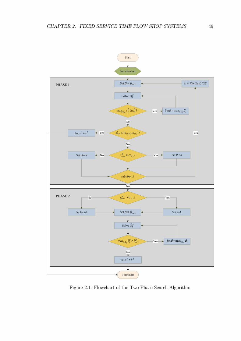
CHAPTER 2. FIXED SERVICE TIME FLOW SHOP SYSTEMS 49
PHASE 1
PHASE 2
Initialization
(ublb)>1?
Yes
Terminate
Set ub=k Set lb=k
Start
2/)( ublbk +=maxSet ββ =
βkQSolve
Yes
?],[ )()1(max kks σσβ−∈
No
No
Set h=k1 Set h=kmaxSet ββ =
jmaxSet βββIj∉=
βss =*Set
YesNo
No Yes
Yes
Yes
jIj βββ∉= maxSet
?)(max ks σβ >
βhQSolve
No
?)(max ks σβ >
No
βss ˆSet * =
?max βββ mjIj ss ≥∉
?ˆˆmax βββ mjIj ss ≥∉
Figure 2.1: Flowchart of the Two-Phase Search Algorithm
CHAPTER 2. FIXED SERVICE TIME FLOW SHOP SYSTEMS 50
of JR. Otherwise, we proceed with Phase 2 and solve a series of di¤erentiable
subproblemsnQ�k
o�=�max�=��k
with the solution methodology described in Subsection
2.5.2.1.
In the worst case, this algorithm solves M dlog2Ne of Q�k problems involving
two nonlinear equations and two unknowns, andM of Q�k problems involving one
nonlinear equation and one unknown. Hence, it determines the optimal solution
in a �nite number of steps.
2.6 Numerical Study
Let us consider an M -machine �ow shop system processing an identical set of N
jobs. The service cost �j(sj) at machine j is given as
�j(sj) =�jsj
(2.117)
for some constant �j where � in (2.69) is set to 1. The completion-time cost for
job Ci, on the other hand, is given by a cost de�ned as
�i(xi;M) = 10(xi;M � ai)2: (2.118)
Note that the costs given by (2.117) and (2.118) satisfy Assumptions 2.1 (as
well as 2.3) and 2.2 respectively.
2.6.1 Veri�cation of the Waiting Characteristics
To illustrate the waiting characteristics of �xed service time �ow systems de-
rived in Section 2.2, we �rst consider the system, where ten jobs are to be
processed in a �ow shop of four machines, i.e., N = 10 and M = 4, with the
costs given by (2.117) and (2.118). The arrival times of the jobs are given as
a = [0:0; 2:3; 2:4; 4:9; 5:0; 5:5; 9:0; 9:5; 11:0; 13:0], while the � parameter vector in
CHAPTER 2. FIXED SERVICE TIME FLOW SHOP SYSTEMS 51
(2.117) is given as � = [100; 50; 200; 100]. The service times on these four ma-
chines are bounded below by S = [0:20; 0:20; 0:30; 0:35], while the due dates for
job completions are set to in�nity, i.e. , di =1 for all i = 1; :::; 10.
The optimal service times are found to be s� = [0:4942; 0:3495; 0:5593; 0:4942]
yielding the optimal cost of 1329:01 units. Hence, for the optimal solution, the
�rst machine, as in all �xed service time �ow shop systems, turns out to be a
local bottleneck, while the third machine is the global bottleneck, and there are
no other local bottleneck machines. Therefore, the system can be divided into
two �ushing portions: one is formed of the �rst and the second machines, and
the other is formed of the third and the fourth machines. From Lemma 2.1, we
expect to see no waiting in front of the second and the fourth machines. Given
the arrival times a, the minimums of the average interarrival times are evaluated
as � = [1; 2:3; 0:1; 1:3; 0:1; 0:3; 1:34; 0:5; 1; 1:�3]. From Lemma 2.3, we expect jobs
fC3; C5; C6g to wait in front of the �rst machine, because �3 = �5 � �6 < s�1.
They are also expected to wait in front of the third machine, the downstream local
(and global) bottleneck machine, as stated in Lemma 2.2. Since s�1 � �8 < s�3,
job C8 is expected to wait only in front of the third machine. Finally, since jobs
fC1; C2; C4; C7; C9; C10g are not expected to wait in front of the third (globalbottleneck) machine because s�3 � �9 � �4 � �10 � �7 � �2 � �1, they are
expected to observe no waiting in the system. The optimal departure times
resulting from operating with optimal service times s� are given in Table 2.1
verifying the realization of expected waiting characteristics. (Note that boldface
numbers denote waiting after departure.)
To observe its convergence behavior, the optimization problem R is also solved
for the above system with the subgradient descent algorithm. The service times
are initially set to their lower bounds s0j = Sj for all j = 1; :::; 4. The termination
tolerance � is given to be 10�8 and the step size at iteration k is given as �k =0:002k.
The implemented distance metric is given as
d�sk; sk�1
�= max
j=1;:::;M
��skj � sk�1j
�� : (2.119)
The service times in the �rst twenty iterations are shown in Figure 2.2.
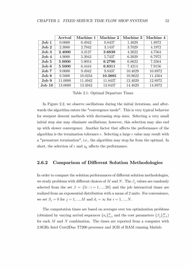
CHAPTER 2. FIXED SERVICE TIME FLOW SHOP SYSTEMS 52
Arrival Machine 1 Machine 2 Machine 3 Machine 4Job 1 0.0000 0.4942 0.8437 1.4029 1.8972Job 2 2.3000 2.7942 3.1437 3.7029 4.1972Job 3 2:4000 3.3127 3:6838 4.2622 4.7564Job 4 4.9000 5.3942 5.7437 6.3029 6.7972Job 5 5:0000 5.9054 6:2796 6.8622 7.3564Job 6 5:5000 6.4444 6:8311 7.4214 7.9156Job 7 9.0000 9.4942 9.8437 10.4029 10.8972Job 8 9.5000 10.0234 10:3885 10.9622 11.4564Job 9 11.0000 11.4942 11.8437 12.4029 12.8972Job 10 13.0000 13.4942 13.8437 14.4029 14.8972
Table 2.1: Optimal Departure Times
In Figure 2.2, we observe oscillations during the initial iterations, and after-
wards the algorithm enters the "convergence mode". This is very typical behavior
for steepest descent methods with decreasing step sizes. Selecting a very small
initial step size may eliminate oscillations; however, this selection may also end
up with slower convergence. Another factor that a¤ects the performance of the
algorithm is the termination tolerance �. Selecting a large � value may result with
a "premature termination", i.e., the algorithm may stop far from the optimal. In
short, the selection of � and �k a¤ects the performance.
2.6.2 Comparison of Di¤erent Solution Methodologies
In order to compare the solution performances of di¤erent solution methodologies,
we study problems with di¤erent choices ofM andN . The �j values are randomly
selected from the set � = f5i : i = 1; :::; 20g and the job interarrival times arerealized from an exponential distribution with a mean of 2 units. For convenience,
we set Sj = 0 for j = 1; :::;M and di =1 for i = 1; :::; N .
The computation times are based on averages over ten optimization problems
(obtained by varying arrival sequences faigNi=1 and the cost parameters f�jgMj=1)for each M and N combination. The times are reported from a computer with
2.0GHz Intel Core2Duo T7200 processor and 2GB of RAM running Matlab.
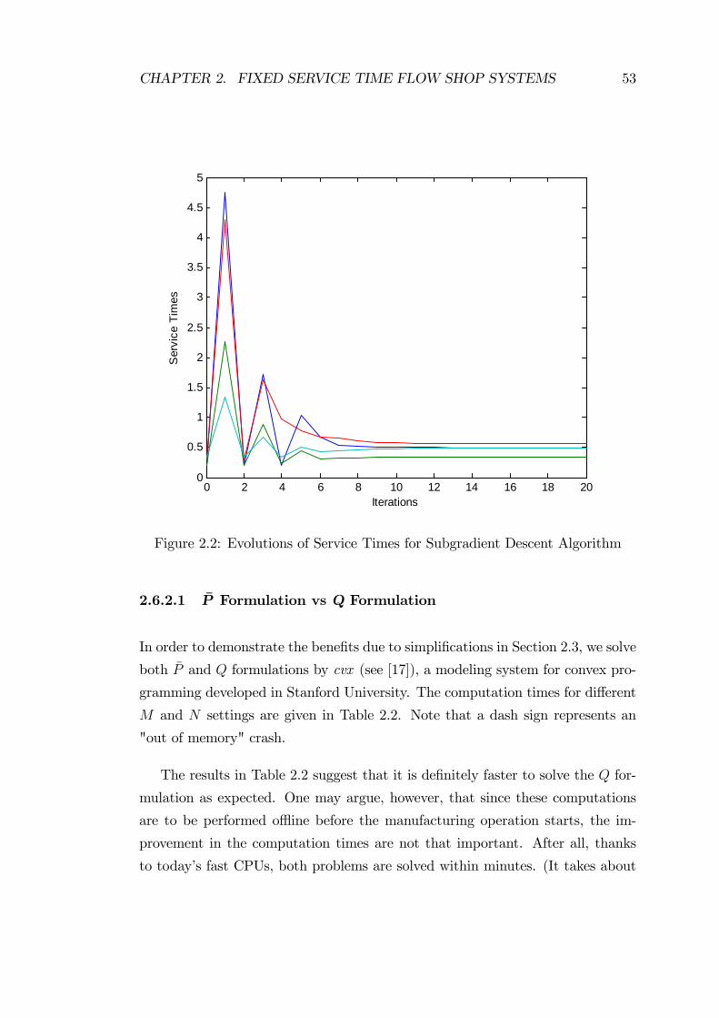
CHAPTER 2. FIXED SERVICE TIME FLOW SHOP SYSTEMS 53
0 2 4 6 8 10 12 14 16 18 200
0.5
1
1.5
2
2.5
3
3.5
4
4.5
5
Iterations
Ser
vice
Tim
es
Figure 2.2: Evolutions of Service Times for Subgradient Descent Algorithm
2.6.2.1 �P Formulation vs Q Formulation
In order to demonstrate the bene�ts due to simpli�cations in Section 2.3, we solve
both �P and Q formulations by cvx (see [17]), a modeling system for convex pro-
gramming developed in Stanford University. The computation times for di¤erent
M and N settings are given in Table 2.2. Note that a dash sign represents an
"out of memory" crash.
The results in Table 2.2 suggest that it is de�nitely faster to solve the Q for-
mulation as expected. One may argue, however, that since these computations
are to be performed o ine before the manufacturing operation starts, the im-
provement in the computation times are not that important. After all, thanks
to today�s fast CPUs, both problems are solved within minutes. (It takes about
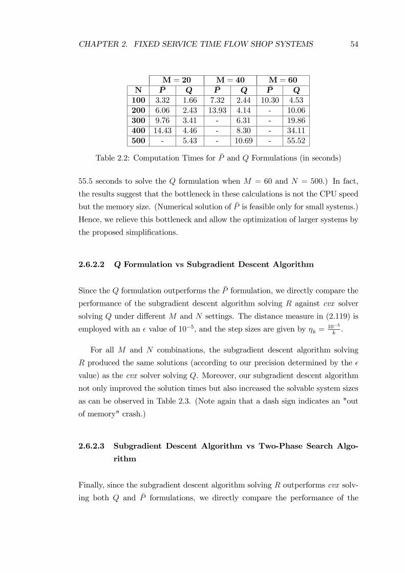
CHAPTER 2. FIXED SERVICE TIME FLOW SHOP SYSTEMS 54
M = 20 M = 40 M = 60N �P Q �P Q �P Q100 3.32 1.66 7.32 2.44 10.30 4.53200 6.06 2.43 13.93 4.14 - 10.06300 9.76 3.41 - 6.31 - 19.86400 14.43 4.46 - 8.30 - 34.11500 - 5.43 - 10.69 - 55.52
Table 2.2: Computation Times for �P and Q Formulations (in seconds)
55:5 seconds to solve the Q formulation when M = 60 and N = 500.) In fact,
the results suggest that the bottleneck in these calculations is not the CPU speed
but the memory size. (Numerical solution of �P is feasible only for small systems.)
Hence, we relieve this bottleneck and allow the optimization of larger systems by
the proposed simpli�cations.
2.6.2.2 Q Formulation vs Subgradient Descent Algorithm
Since the Q formulation outperforms the �P formulation, we directly compare the
performance of the subgradient descent algorithm solving R against cvx solver
solving Q under di¤erent M and N settings. The distance measure in (2.119) is
employed with an � value of 10�5, and the step sizes are given by �k =10�5
k.
For all M and N combinations, the subgradient descent algorithm solving
R produced the same solutions (according to our precision determined by the �
value) as the cvx solver solving Q. Moreover, our subgradient descent algorithm
not only improved the solution times but also increased the solvable system sizes
as can be observed in Table 2.3. (Note again that a dash sign indicates an "out
of memory" crash.)
2.6.2.3 Subgradient Descent Algorithm vs Two-Phase Search Algo-
rithm
Finally, since the subgradient descent algorithm solving R outperforms cvx solv-
ing both Q and �P formulations, we directly compare the performance of the
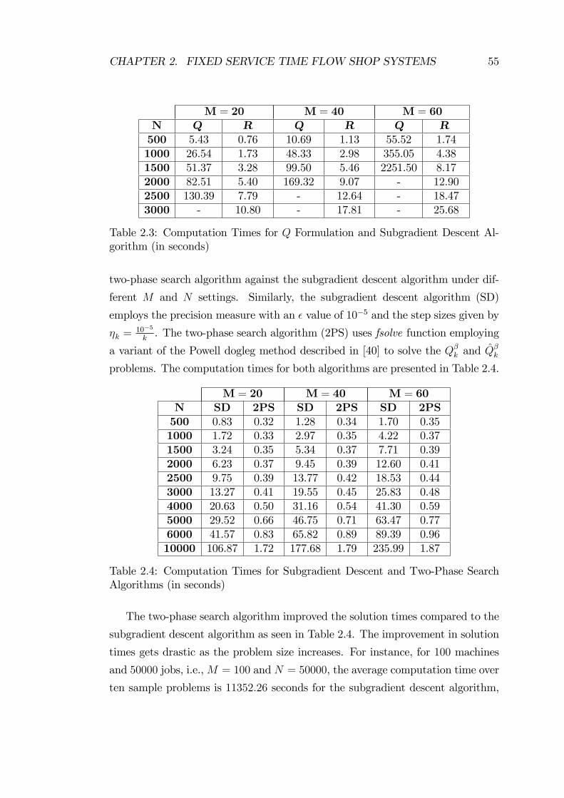
CHAPTER 2. FIXED SERVICE TIME FLOW SHOP SYSTEMS 55
M = 20 M = 40 M = 60N Q R Q R Q R500 5.43 0.76 10.69 1.13 55.52 1.741000 26.54 1.73 48.33 2.98 355.05 4.381500 51.37 3.28 99.50 5.46 2251.50 8.172000 82.51 5.40 169.32 9.07 - 12.902500 130.39 7.79 - 12.64 - 18.473000 - 10.80 - 17.81 - 25.68
Table 2.3: Computation Times for Q Formulation and Subgradient Descent Al-gorithm (in seconds)
two-phase search algorithm against the subgradient descent algorithm under dif-
ferent M and N settings. Similarly, the subgradient descent algorithm (SD)
employs the precision measure with an � value of 10�5 and the step sizes given by
�k =10�5
k. The two-phase search algorithm (2PS) uses fsolve function employing
a variant of the Powell dogleg method described in [40] to solve the Q�k and Q�k
problems. The computation times for both algorithms are presented in Table 2.4.
M = 20 M = 40 M = 60N SD 2PS SD 2PS SD 2PS500 0.83 0.32 1.28 0.34 1.70 0.351000 1.72 0.33 2.97 0.35 4.22 0.371500 3.24 0.35 5.34 0.37 7.71 0.392000 6.23 0.37 9.45 0.39 12.60 0.412500 9.75 0.39 13.77 0.42 18.53 0.443000 13.27 0.41 19.55 0.45 25.83 0.484000 20.63 0.50 31.16 0.54 41.30 0.595000 29.52 0.66 46.75 0.71 63.47 0.776000 41.57 0.83 65.82 0.89 89.39 0.9610000 106.87 1.72 177.68 1.79 235.99 1.87
Table 2.4: Computation Times for Subgradient Descent and Two-Phase SearchAlgorithms (in seconds)
The two-phase search algorithm improved the solution times compared to the
subgradient descent algorithm as seen in Table 2.4. The improvement in solution
times gets drastic as the problem size increases. For instance, for 100 machines
and 50000 jobs, i.e.,M = 100 and N = 50000, the average computation time over
ten sample problems is 11352:26 seconds for the subgradient descent algorithm,
CHAPTER 2. FIXED SERVICE TIME FLOW SHOP SYSTEMS 56
while this value is only 33:06 seconds for the two-phase search algorithm.
2.7 Conclusion
In this chapter, we considered the deterministic �ow shop systems, where the
service times of the machines are �xed known values or set only once and can
not be altered between processes. The arrival times of the jobs and their associ-
ated deadlines were assumed to be known a priori. A standard solution method
based on the linearization of the max constraints yielded a convex optimization
problem with high memory requirements. In order to derive an equivalent convex
optimization problem with lower memory requirements, a set of waiting and com-
pletion time characteristics for �xed service time �ow shop systems was derived
and exploited. Basically, it was shown that jobs do not wait at the downstream of
the machine with highest service time and a certain job always waits at this ma-
chine if it observes waiting in the system. Exploiting these results, job completion
times were shown to be represented as a function of the service times of the ma-
chines in the system. This representation was then incorporated into the problem
to derive a simpli�ed equivalent convex optimization problem through eliminating
many of its constraints. As shown by the numerical study, the resulting simpli�ed
convex optimization problem had signi�cantly lower memory requirements and
somewhat lower solution times. However, since this formulation still required a
convex programming problem solver, which may not be available in small man-
ufacturing companies, and needed several GB�s of memory for large problems,
we also proposed an alternative convex formulation which is not everywhere dif-
ferentiable, and a subgradient descent solution method employing subgradients
for directions. While deriving this alternative convex optimization problem along
with its subgradient solution method, we employed an alternative representation
of job completion times, again as the function of the service times of all machines
in the system, derived through further exploitation of the waiting and completion
time characteristics of �xed service time �ow shop systems. As demonstrated by
the numerical study, substantial improvements in solution times and solvable sys-
tem sizes were achieved by the proposed subgradient descent solution method.
CHAPTER 2. FIXED SERVICE TIME FLOW SHOP SYSTEMS 57
Finally, we focused on a speci�c service cost structure which allowed us to sort
the optimal service times and to de�ne di¤erentiable subproblems leading to a
two-phase search algorithm. This new search algorithm, which is guaranteed to
�nd the optimal service times in a �nite number of iterations, was shown to im-
prove the solution times drastically compared to the subgradient descent solution
method by the numerical study.
Chapter 3
Service Time Optimization of
Mixed Line Flow Shop Systems
In this chapter, we consider deterministic �ow shop systems formed of fully con-
trollable, initially controllable, and uncontrollable machines processing identical
jobs with known arrival times and deadlines. We note that mixed line �ow shop
systems with no fully controllable machines turn out to be the �xed service time
�ow shop systems that were analyzed comprehensively in Chapter 2. Hence,
throughout the chapter, we assume that there exists at least one fully control-
lable machine in the system. In fact, analysis of mixed line �ow shops exten-
sively exploits the structural properties of �xed service time �ow shop systems
presented in Chapter 2. However, including fully controllable machines in the
system allows for some more optimal waiting characteristics which lead to new
solution methodologies di¤erent from the ones developed for �xed service time
�op shop systems. Hence, we devote a new chapter to mixed line �ow shops
systems. The cost function we consider consists of service costs at fully and ini-
tially controllable machines, which are dependent on service times, and regular
completion-time costs for jobs. Based on the same reasoning in Chapter 2, we as-
sume that faster services increase service costs, while slower services increase the
regular completion-time costs and/or leading to failures in accomplishing jobs
within their deadlines. This trade-o¤ is what makes the problem challenging
58
CHAPTER 3. MIXED LINE FLOW SHOP SYSTEMS 59
and our objective is to determine the cost-minimizing service times at fully and
initially controllable machines.
In this chapter, we �rst formulate a non-convex and non-di¤erentiable opti-
mization problem which can be solved by the convex formulation derived through
the standard method of linearization on the max constraints. However, high
memory requirement of the resulting convex formulation limits its solution only
to small systems. Motivated by the need for solving larger systems within rea-
sonable solution times, we present a set of optimal waiting characteristics for
such �ow shop systems and employ them to develop e¢ cient solution method-
ologies. Mainly, under some cost assumptions, we show that jobs do not wait
on the optimal sample path at the downstream of the �rst fully controllable ma-
chine. Utilizing this property, we derive simpli�ed equivalent convex optimization
problems. For the �ow shop systems formed of only fully controllable and un-
controllable machines, the associated simpli�ed equivalent convex optimization
problem is then decomposed by a "forward in time" algorithm into smaller con-
vex optimization problems under an additional strict convexity assumption on
the completion-time costs.
The rest of this chapter is organized as follows: We formulate a non-convex
and non-di¤erentiable optimization problem and present a convex programming
formulation derived through linearization in Section 3.1. In Section 3.2, we derive
a set of waiting characteristics of such systems and show that, on the optimal
sample path, no waiting is observed after the �rst fully controllable machine of
the system. In Section 3.3, we develop simpli�ed convex programming formu-
lations by employing the no-wait property derived in Section 3.2. For the �ow
shop systems of fully controllable and uncontrollable machines, a forward de-
composition algorithm is presented in Section 3.4 to decompose the associated
simpli�ed convex optimization problem derived in Section 3.3 into smaller convex
optimization problems with linear constraints. In Section 3.5, a numerical study
is held to visualize the optimal waiting characteristics derived in Section 3.2, to
demonstrate the bene�ts of the simpli�cation and the decomposition in terms
of solution performances, and to compare the forward decomposition algorithm
against another algorithm (applicable to a special case of our model) from the
CHAPTER 3. MIXED LINE FLOW SHOP SYSTEMS 60
literature through a set of example systems. Analysis of the e¤ects of replacing an
initially controllable machine with a fully controllable machine and the locations
of fully controllable machines on the optimal cost, and service and completion-
time costs on the optimal service times are also included in Section 3.5. Finally,
Section 3.6 concludes the chapter.
3.1 Problem Formulation
The notation used throughout the chapter is as follows:
Decision Variables:
xi;j : departure time of job i from machine j.
si;j : service time of job i at fully controllable machine j.
sj : service time at initially controllable machine j.
Parameters:
M : number of machines in the system.
N : number of jobs that arrive at the system.
ai : arrival time of job i.
di : deadline for the completion of job i.
�sj : service time at uncontrollable machine j.
Sj : lower bound for the service time at machine j.
SF : index set of fully controllable machines in the system.
SI : index set of initially controllable machines in the system.
SU : index set of uncontrollable machines in the system.
�j(sj) : total service cost over all jobs at initially controllable machine j.
�j(si;j) : service cost of job i at fully controllable machine j.
�i(xi;M) : completion-time cost for job i.
CHAPTER 3. MIXED LINE FLOW SHOP SYSTEMS 61
Let us consider an M -machine �ow shop system. A sequence of N identical
jobs arrive at the system at known times 0 � a1 � a2 � ::: � aN and are processedin all machines sequentially. We denote these jobs by fCigNi=1 and assign them jobcompletion deadlines as fdigNi=1. Machines, with bu¤ers of in�nite sizes, processone job at a time on a �rst-come �rst-served non-preemptive basis (i.e. a job in
service cannot be interrupted until its service completion). The system consists
of fully controllable machines, where the service times can be adjusted before
each process, initially controllable machines, where the service time are set only
once before arrival of the �rst job, and uncontrollable machines, where the service
times are �xed and foreknown. We de�ne the sets SF , SI , and SU as the index
sets of the fully controllable, initially controllable, and uncontrollable machines,
respectively. Then, the service times at each machine j 2 SF are denoted byfsi;jgNi=1, while the service times are denoted by sj and �sj at each machine j 2 SIand j 2 SU , respectively.
To keep the notation simple and to make the rest of the chapter more read-
able, without loss of generality, we treat the uncontrollable machines as if they
are initially controllable machines as done in Chapter 2 and we study the �ow
shop systems consisting only of fully and initially controllable machines. We ac-
knowledge that the results of such system are applicable to �ow shop systems
including also uncontrollable machines.
We de�ne xi;j as the departure time of job Ci from machine j and consider the
discrete-event optimal control problem, denoted by PM , which has the following
form:
PM : minsi;j ;sj�Sji=1;:::;Nj=1;:::;M
(JM =
NXi=1
Xj2SF
�j(si;j) +Xj2SI
�j(sj) +
NXi=1
�i(xi;M)
)(3.1)
subject to
xi;j = max (xi;j�1; xi�1;j) + si;j; j 2 SF (3.2)
xi;j = max (xi;j�1; xi�1;j) + sj; j 2 SI (3.3)
CHAPTER 3. MIXED LINE FLOW SHOP SYSTEMS 62
xi;M � di (3.4)
xi;0 = ai; x0;j = �1; 8j (3.5)
for i = 1; :::; N . In this formulation, �j denotes the service cost at machine j, and
�i denotes the completion-time cost for job Ci.
Similarly as in Chapter 2, the lower bounds on service times at machines
may prevent some jobs from meeting their associated deadlines, therefore cause
infeasibility. Here, we will consider the case where a feasible solution exists for the
optimization problem PM . If that is not the case, then a separate job admission
control problem has to precede our analysis so as to reject some jobs and lead to
a feasible problem as in [29], which is not considered here.
The following assumptions are necessary to make the problem somewhat more
tractable while preserving the originality of the problem.
Assumption 3.1 : �j(�), for j = 1; :::;M , is continuously di¤erentiable,
monotonically decreasing, and strictly convex.
Assumption 3.2 : �i(�), for i = 1; :::; N , is continuously di¤erentiable,
monotonically increasing, and convex.
Note that for the costs satisfying these assumptions, longer services will de-
crease the service costs, while possibly increasing the completion times, hence,
the completion-time costs.
By replacing the constraints xi;j = max (xi;j�1; xi�1;j) + si;j in (3.2) by the
constraints
xi;j � xi;j�1 + si;j;
xi;j � xi�1;j + si;j;
CHAPTER 3. MIXED LINE FLOW SHOP SYSTEMS 63
and the constraints xi;j = max (xi;j�1; xi�1;j) + sj in (3.3) by the constraints
xi;j � xi;j�1 + sj;
xi;j � xi�1;j + sj;
resulting with the convex optimization problem �PM de�ned as
�PM : minsi;j ;sj�Sj
xi;ji=1;:::;Nj=1;:::;M
(�JM =
NXi=1
Xj2SF
�j(si;j) +Xj2SI
�j(sj) +
NXi=1
�i(xi;M)
)
subject to
xi;j � xi;j�1 + si;j; j 2 SF (3.6)
xi;j � xi�1;j + si;j; j 2 SF (3.7)
xi;j � xi;j�1 + sj; j 2 SI (3.8)
xi;j � xi�1;j + sj; j 2 SI (3.9)
xi;M � di (3.10)
xi;0 = ai, x0;j = �1; 8j (3.11)
for all i = 1; :::; N .
Since the feasible set of the convex optimization problem �PM contains the
feasible set of the optimization problem PM , its optimal cost �J�M is upper bounded
by the optimal cost of PM denoted by J�M , i.e., �J�M � J�M . It can be easily
veri�ed that an optimal service vector �s� for the convex optimization problem�PM is also optimal for the problem PM . Hence, by solving �PM we can obtain an
optimal solution for PM . Moreover, any optimal solution for PM along with its
corresponding departure times constitute an optimal solution for �PM .
In the next section, we show that no waiting is observed after the �rst fully
controllable machine, a property that is needed to simplify the optimization prob-
lem PM .
CHAPTER 3. MIXED LINE FLOW SHOP SYSTEMS 64
3.2 Waiting Characteristics of the Optimal
Sample Path
The machines in the �ow shop can be decomposed into portions formed of sequen-
tially located same type (fully controllable or initially uncontrollable) of machines.
De�nition 3.1 A contiguous set of machines fu; :::; vg form an initially control-lable (or a fully controllable) portion if
1. Machine (u�1), if exists, is a fully controllable (or an initially controllable)machine;
2. Machines fu; :::; vg are initially controllable (or fully controllable) machines;
3. Machine (v+1), if exists, is a fully controllable (or an initially controllable)
machine.
We analyze the initially controllable and fully controllable portions separately
in the following subsections.
3.2.1 Initially Controllable Portions
Initially controllable portions can be treated as �xed service time �ow shop sys-
tems previously studied in Chapter 2; therefore, the results therein are applicable.
Hence, skipping the proofs, we borrow the following three lemmas from Chap-
ter 2 and adapt them to initially controllable portions. The counterpart of the
global bottleneck machine in �xed service time �ow shop systems is called as the
retarding machine of the initially controllable portion de�ned as follows:
De�nition 3.2 Let machines fu; :::; vg form an initially controllable portion.
The machine m with the highest service time (and the most upstream in case
of a tie) satisfying m = min fk : sk = maxj=u;:::;v sjg is called as the retardingmachine of this portion.
CHAPTER 3. MIXED LINE FLOW SHOP SYSTEMS 65
The arrival time of job Ck at the initially controllable portion formed of ma-
chines fu; :::; vg is given as xk;u�1, and the average interarrival time between jobsCk and Cl at this portion is given as
�lk =xk;u�1 � xl;u�1
k � l ; (3.12)
where l < k.
The minimum of the average interarrival times for job Ck at this initially
controllable portion is, then, de�ned as
�k =
8<: 1; k = 1
minl=1;:::;k�1
�lk; k > 1(3.13)
and, according to the following lemma, it allows us to determine whether a job
waits or not at the retarding machine m.
Lemma 3.1 A job Ck waits for service at the retarding machine m if and only
if �k < sm.
At this point, we borrow the following two de�nitions from Chapter 2 and
decompose the jobs into blocks according to their waiting characteristics at some
machine j.
De�nition 3.3 A contiguous set of jobs fCigni=k is said to form a block at ma-
chine j if
1) Jobs Ck and Cn+1 (if exists) do not wait at machine j, i.e., xk;j�1 � xk�1;jand xn+1;j�1 � xn;j;
2) Jobs fCigni=k+1 wait at machine j, i.e., xi;j�1 < xi�1;j for i = k + 1; :::; n.
De�nition 3.4 A partition of jobs into blocks is called a block structure.
CHAPTER 3. MIXED LINE FLOW SHOP SYSTEMS 66
According to Lemma 3.1, one could evaluate �k values for all jobs Ck and
compare them to the service time of the retarding machine to determine the
block structure. The following lemma, however, presents a simpler way.
Lemma 3.2 If jobs fCigni=k form a block at the retarding machine m, then,
�ki < sm
is satis�ed for all i = k + 1; :::; n.
Being the counterpart of global bottleneck machine in �xed service time �ow
shop systems, no waiting is observed after the retarding machine. Hence, the de-
parture times from initially controllable portions can be determined as presented
in the next lemma.
Lemma 3.3 For the initially controllable portion fu; :::; vg, the departure timeof job Ci is given by
xi;v = max
xi;u�1 +
vXk=u
sk; xi�1;v + sm
!;
where x0;u�1 = �1 and sm = maxk=u;:::;v sk is the service time of the retarding
machine.
Before proceeding with the next lemma, which states that no waiting is ob-
served at initially controllable portions downstream to a fully controllable ma-
chine, let us de�ne xN+1;j =1 for all j = 1; :::;M .
Lemma 3.4 Let machines fu; :::; vg form an initially controllable portion. If
u > 1, i.e., if there is a fully controllable machine upstream to machine u, then,
on the optimal sample path, jobs do not wait at these machines, i.e., x�i;j�1 � x�i�1;jfor all i = 1; :::; N and j = u; :::; v.
CHAPTER 3. MIXED LINE FLOW SHOP SYSTEMS 67
Proof. Let machine m be the retarding machine of the initially controllable
portion fu; :::; vg. Since sm = maxj=u;:::;v sj, we may deduce from Lemma 3.1
that if a job waits for service at some machine in the initially controllable portion
fu; :::; vg, then it also waits for service at the retarding machine m. Hence, toprove the statement of lemma, it su¢ ces to show that jobs do not wait at the
retarding machine m.
(By Induction) Since the �rst job does not wait at any machine, we have the
basis for the induction. For a contradiction in the inductive step, let us assume
that, on the optimal sample path, jobs fCigki=1 do not wait while the job Ck+1waits for service at the retarding machine m.
Let jobs fCigni=k form the block in which job Ck+1 resides at the retarding
machine m. Then, by Lemma 3.3, we have
x�i;u�1 +vXj=u
s�j < x�i�1;v + s
�m (3.14)
for i = k + 1; :::; n and
x�n+1;u�1 +vXj=u
s�j � x�n;v + s�m: (3.15)
By Lemma 3.2 and from (3.12), since job Ck+1 resides in the block started by job
Ck, we also have ��kk+1
��= x�k+1;u�1 � x�k;u�1 < s�m: (3.16)
Moreover, from (3.2), we have
x�k+1;u�1 � x�k;u�1 + s�k+1;u�1: (3.17)
It follows from (3.16) and (3.17) that
s�k+1;u�1 < s�m: (3.18)
CHAPTER 3. MIXED LINE FLOW SHOP SYSTEMS 68
If x�n+1;u�2 � x�n;u�1, we have from (3.2) that
x�n+1;u�1 = x�n;u�1 + s
�n+1;u�1: (3.19)
Since job Cn+1 does not wait at machinem, from (3.12) and (3.13), and by Lemma
3.1, we have ��nn+1
��= x�n+1;u�1 � x�n;u�1 � s�m: (3.20)
It follows from (3.19) and (3.20) that
s�n+1;u�1 � s�m: (3.21)
Hence, it follows from (3.18) and (3.21) that if x�n+1;u�2 � x�n;u�1, then
s�n+1;u�1 > s�k+1;u�1: (3.22)
Next, let us de�ne the perturbed solution as
sj = s�j (3.23)
for all j 2 SI and
si;j =
8>><>>:s�i;j +�1; i = k + 1; j = u� 1s�i;j ��2; i = n+ 1; j = u� 1s�i;j; otherwise
(3.24)
for all i = 1; :::; N and j 2 SF where the positive perturbation �1 and the non-
negative perturbation �2 are de�ned as
�1 =
(minf s
�n+1;u�1�s�k+1;u�1
2;�ag; x�n+1;u�2 � x�n;u�1
minfx�n+1;u�2 � x�n;u�1;�ag; x�n+1;u�2 > x�n;u�1(3.25)
�2 =
(minf s
�n+1;u�1�s�k+1;u�1
2;�ag; x�n+1;u�2 � x�n;u�1
0; x�n+1;u�2 > x�n;u�1:
(3.26)
CHAPTER 3. MIXED LINE FLOW SHOP SYSTEMS 69
Note that in (3.25) and (3.26), �a is de�ned as
�a = mini=k+1;:::;n
((x�i�1;v + s
�m)� (x�i;u�1 +
vXj=u
s�j)
):
Since �2 � �1 from (3.25) and (3.26), then we have from (3.22) and (3.24)
that
sn+1;u�1 = s�n+1;u�1 ��2 � s�k+1;u�1 +�1 = sk+1;u�1 � Su�1; (3.27)
therefore, our perturbed solution is a feasible solution for the optimization prob-
lem PM .
On this alternative sample path, the perturbation does not a¤ect the jobs
before Ck+1 and the machines before (u � 1). Hence, the perturbed departures,denoted by xi;j�s, satisfy
xi;j = x�i;j (3.28)
for all i = 1; :::; k and j = 1; :::;M , or i = k + 1; :::; N and j = 1; :::; u � 2. We,next, determine the e¤ects of this perturbation on xi;j�s for all i = k + 1; :::; N
and j = u� 1; :::;M . First, we show, by induction, that
xi;u�1 � x�i;u�1 +�1
for all i = k + 1; :::; n. From (3.2), (3.24), and (3.28),
xk+1;u�1 = max (xk+1;u�2; xk;u�1) + sk+1;u�1
= max�x�k+1;u�2; x
�k;u�1
�+ s�k+1;u�1 +�1
= x�k+1;u�1 +�1: (3.29)
Next, let us assume that
xr;u�1 � x�r;u�1 +�1 (3.30)
CHAPTER 3. MIXED LINE FLOW SHOP SYSTEMS 70
for some r 2 fk + 1; :::; n� 1g. Then, from (3.2), (3.24), (3.28), and (3.30),
xr+1;u�1 = max (xr+1;u�2; xr;u�1) + sr+1;u�1
� max�x�r+1;u�2; x
�r;u�1 +�1
�+ s�r+1;u�1
� x�r+1;u�1 +�1:
Hence, we have
xi;u�1 � x�i;u�1 +�1 (3.31)
for all i = k + 1; :::; n.
From (3.14), (3.23), (3.25), (3.28), (3.29), and by Lemma 3.3, the departure
time of the job Ck+1 from the initially controllable portion formed of machines
fu; :::; vg for the perturbed solution is given as
xk+1;v = max
xk+1;u�1 +
vXj=u
sj; xk;v + sm
!
= max
x�k+1;u�1 +�1 +
vXj=u
s�j ; x�k;v + s
�m
!= x�k+1;v (3.32)
and starting with (3.32), we recursively obtain from (3.31) that
xi;v = max
xi;u�1 +
vXj=u
sj; xi�1;v + sm
!
= max
x�i;u�1 +�1 +
vXj=u
s�j � "i; x�i�1;v + s�m
!= x�i;v (3.33)
for all i = k + 2; :::; n where "i � 0. Hence, the perturbation does not a¤ect thedeparture times of the jobs fCigni=k+1 at machines fv; :::;Mg resulting in
xi;M = x�i;M (3.34)
for all i = 1; :::; n.
CHAPTER 3. MIXED LINE FLOW SHOP SYSTEMS 71
Further, from (3.2), (3.24), (3.25), (3.26), (3.28), and (3.31), the departure
time of the job Cn+1 from machine (u � 1) for the perturbed solution is writtenas
xn+1;u�1 = max (xn+1;u�2; xn;u�1) + sn+1;u�1
� max�x�n+1;u�2; x
�n;u�1 +�1
�+ s�n+1;u�1 ��2
� x�n+1;u�1; (3.35)
therefore, from (3.23), (3.33), (3.35), and by Lemma 3.3, the departure time of
this job from initially controllable portion fu; :::; vg is given by
xn+1;v = max
xn+1;u�1 +
vXj=u
sj; xn;v + sm
!
� max
x�n+1;u�1 +
vXj=u
s�j ; x�n;v + s
�m
!� x�n+1;v: (3.36)
Hence, from (3.2), (3.3), (3.23), (3.24), and (3.36)
xi;j � x�i;j (3.37)
for all i = n + 1; :::; N , j = v; :::;M indicating the possibility of decrease in
the departure times of the jobs fCigNi=n+1 at machines fv; :::;Mg due to theperturbation.
Let us denote the cost of this alternative solution as J . Then, from (3.23),
(3.24), (3.34), and (3.37), the cost variation, denoted by �J = J � J�M , is givenby
�J =��u�1(s
�k+1;u�1 +�1)� �u�1(s�k+1;u�1)
����u�1(s
�n+1;u�1)� �u�1(s�n+1;u�1 ��2)
�+
NXi=n+1
��i(xi;M)� �i(x�i;M)
�:
CHAPTER 3. MIXED LINE FLOW SHOP SYSTEMS 72
Since, by Assumption 3.1, the service cost �u�1 is monotonically decreasing and
strictly convex, from (3.22), (3.25), and (3.26),
��u�1(s
�k+1;u�1 +�1)� �u�1(s�k+1;u�1)
����u�1(s
�n+1;u�1)� �u�1(s�n+1;u�1 ��2)
�< 0:
(3.38)
Moreover, since, by Assumption 3.2, the completion-time cost �i is monotonically
increasing, from (3.37),
NXi=n+1
[�i(xi;M)� �i(x�i;M)] � 0: (3.39)
From (3.38) and (3.39), we have �J < 0 which contradicts the optimality as-
sumption. Hence, the result follows.
In this subsection, we showed that no waiting is observed at the initially
controllable portions downstream to a fully controllable machine. In the following
subsection, we show that the �rst fully controllable machine is the only fully
controllable machine that allows for waiting, i.e., no waiting is observed in the
�ow shop system after the �rst fully controllable machine.
3.2.2 Fully Controllable Portions
Applying calculus of variations techniques (see in [25]) on the convex optimization
problem �PM , we obtain a set of necessary conditions for optimality. Let us start
with introducing the Lagrangian multipliers �i;j, �i;j, �i;j, �j, and i to form the
CHAPTER 3. MIXED LINE FLOW SHOP SYSTEMS 73
augmented cost
JA =
NXi=1
Xj2SF
�j(si;j) +Xj2SI
�j(sj) +NXi=1
�i(xi;M)
+NXi=1
Xj2SF
(�i;j [xi;j�1 + si;j � xi;j] + �i;j [xi�1;j + si;j � xi;j])
+NXi=1
Xj2SI
(�i;j [xi;j�1 + sj � xi;j] + �i;j [xi�1;j + sj � xi;j])
+NXi=1
Xj2SF
�i;j (Sj � si;j) +Xj2SI
�j (Sj � sj) +NXi=1
i (xi;M � di) :
As stated earlier, the optimal solution vector s� of PM , together with its
corresponding departure time vector x� form an optimal solution for �PM . Hence,
from the augmented cost formulation, fs�; x�g satisfy the following necessaryconditions for optimality:
1) For i = 1; :::; N and j 2 SF
@JA@si;j
����s�i;j
= �0j(s�i;j) + �
�i;j + �
�i;j � ��i;j = 0; (3.40)
��i;j � 0; ��i;j�x�i;j�1 + s
�i;j � x�i;j
�= 0; (3.41)
��i;j � 0; ��i;j�x�i�1;j + s
�i;j � x�i;j
�= 0; (3.42)
��i;j � 0; ��i;j�Sj � s�i;j
�= 0; (3.43)
s�i;j � Sj; (3.44)
and since �0j(�) < 0 by Assumption 3.1, from (3.40) and (3.43),
��i;j + ��i;j > 0; (3.45)
CHAPTER 3. MIXED LINE FLOW SHOP SYSTEMS 74
and �nally from (3.41), (3.42), and (3.45),
x�i;j = max�x�i;j�1; x
�i�1;j
�+ s�i;j: (3.46)
2) For i = 1; :::; N and j 2 SI
@JA@sj
����s�j
= �0j(s�j) +
NXi=1
���i;j + �
�i;j
�� ��j = 0; (3.47)
��i;j � 0; ��i;j�x�i;j�1 + s
�j � x�i;j
�= 0; (3.48)
��i;j � 0; ��i;j�x�i�1;j + s
�j � x�i;j
�= 0; (3.49)
��j � 0; ��j�Sj � s�j
�= 0; (3.50)
s�j � Sj; (3.51)
and since by Assumption 3.1, �0j(�) < 0, from (3.47) and (3.50),
NXi=1
���i;j + �
�i;j
�> 0: (3.52)
3) For i = 1; :::; N and j = 1; :::;M
�i � 0; �i�x�i;M � di
�= 0; (3.53)
@JA@xi;j
����x�i;j
= 0; (3.54)
leading to
3a) For i = 1; :::; N � 1 and j = 1; :::;M � 1
��i;j + ��i;j = �
�i;j+1 + �
�i+1;j: (3.55)
CHAPTER 3. MIXED LINE FLOW SHOP SYSTEMS 75
3b) For i = 1; :::; N � 1
��i;M + ��i;M = �0i(x
�i;M) + �
�i+1;M + i: (3.56)
3c) For j = 1; :::;M � 1
��N;j + ��N;j = �
�N;j+1: (3.57)
3d)
��N;M + ��N;M = �0N(x
�N;M) + M : (3.58)
The characteristics (3.40)-(3.58) are needed for the proofs that follow.
The following lemma, which establishes the monotonicity property of the op-
timal service times at fully controllable machines, is needed for the contradiction
argument in the proof of Lemma 3.6.
Lemma 3.5 (Monotonicity Property) Let machine j be a fully controllable ma-
chine, i.e., j 2 SF . Then, for some i 2 f2; :::; Ng, if jobs Ci�1 and Ci are inthe same block of the jth machine on the optimal sample path then the optimal
service times satisfy s�i;j � s�i�1;j.
Proof. Let us assume that s�i;j < s�i�1;j. From (3.44), there are two possible
cases:
Case 1: s�i�1;j > s�i;j = Sj: From (3.43), ��i�1;j = 0 and �
�i;j � 0.
Case 2: s�i�1;j > s�i;j > Sj: From (3.43), ��i�1;j = �
�i;j = 0.
From both cases, for the assumption s�i�1;j > s�i;j, we get
��i;j � ��i�1;j � 0: (3.59)
Since jobs Ci�1 and Ci are in the same block of the jth machine on the optimal
CHAPTER 3. MIXED LINE FLOW SHOP SYSTEMS 76
sample path, we have
x�i;j�1 < x�i�1;j: (3.60)
Further, from (3.41), (3.46), and (3.60), we also have
��i;j = 0: (3.61)
From (3.41), (3.48), (3.53), (3.55), (3.56), (3.61), and by Assumption 3.2, we have
��i�1;j + ��i�1;j � ��i;j � ��i;j =
(��i�1;j+1; j < M
�0i�1(x�i�1;M) +
�i�1; j =M
� 0: (3.62)
It follows from (3.40), (3.59), and (3.62) that
�0j(s�i;j)� �0j(s�i�1;j) � 0:
By Assumption 3.1, �0j is monotonically increasing; therefore s�i;j � s�i�1;j, which
contradicts the initial assumption s�i;j < s�i�1;j. Hence, within a block of a machine
j, the optimal service times are non-decreasing in the job index.
In the next lemma, we show that a fully controllable machine prevents bu¤er-
ing in its downstream fully controllable machines.
Lemma 3.6 Let machines h and t, where h < t, be two consecutive fully
controllable machines, possibly separated by the initially controllable portion
fh + 1; :::; t � 1g. On the optimal sample path, no waiting is observed at thefully controllable machine t.
Proof. (By Induction) Since the �rst job does not wait at any machine, we
have the basis for the induction. For a contradiction in the inductive step, let us
assume that, on the optimal sample path, jobs fCigki=1 do not wait while the jobCk+1 waits for service at the fully controllable machine t. Let jobs fCigni=k formthe block in which job Ck+1 resides at the fully controllable machine t. Then, by
Lemma 3.5,
s�n;t � s�k;t (3.63)
CHAPTER 3. MIXED LINE FLOW SHOP SYSTEMS 77
and from the block de�nition,
x�k;t�1 � x�k�1;t; (3.64)
x�n+1;t�1 � x�n;t; (3.65)
x�i;t�1 < x�i�1;t (3.66)
for i = k + 1; :::; n.
Since, by Lemma 3.4, no waiting is observed at initially controllable portions
followed by a fully controllable machine, we have
x�i;t�1 =
(x�i;h +
Pt�1j=h+1 s
�j ; t > h+ 1
x�i;h; t = h+ 1(3.67)
for all i = 1; :::; N . From (3.2), (3.64), (3.66), (3.67), and since job Ck does not
wait at machine t, we have
s�k+1;h � x�k+1;h � x�k;h < s�k;t (3.68)
and
x�n;h < x�k;h +
n�1Xi=k
s�i;t: (3.69)
Similarly, since jobs fCigni=k form a block at machine t, from (3.2), (3.64), (3.65),(3.66), and (3.67), we have
x�n+1;h � x�k;h +nXi=k
s�i;t: (3.70)
If x�n+1;h�1 � x�n;h, from (3.2), (3.63), (3.68), (3.69), and (3.70),
s�k+1;h < s�k;t � s�n;t < s�n+1;h: (3.71)
If t > h+ 1, i.e., if there is an initially controllable portion between machines
h and t, then let us denote the retarding machine of this portion by machine m.
CHAPTER 3. MIXED LINE FLOW SHOP SYSTEMS 78
As established in Lemma 3.4, jobs do not wait at the initially controllable portion
fh+1; :::; t�1g; hence, by Lemma 3.1, and from (3.12), (3.13), (3.63), and (3.68),
s�n;t � s�k;t > x�k+1;h � x�k;h � s�m: (3.72)
Further, from (3.2), (3.65), (3.66), (3.67), and (3.72),
x�n+1;t�1 = x�n+1;h +
t�1Xj=h+1
s�j > x�n;t�1 + s
�m: (3.73)
Next, let us de�ne the perturbed solution as
sj = s�j (3.74)
for j 2 SI and
si;j =
8>><>>:s�i;j +�1; i = k + 1; j = h
s�i;j ��2; i = n+ 1; j = h
s�i;j; otherwise
(3.75)
for all i = 1; :::; N and j 2 SF where the perturbations �1 and �2 are given as
�1 =
8>>>><>>>>:minf s
�n+1;h�s�k+1;h
2;�ag; x�n+1;h�1 � x�n;h; t = h+ 1
minf s�n+1;h�s�k+1;h
2;�a;�bg; x�n+1;h�1 � x�n;h; t > h+ 1
minfx�n+1;h�1 � x�n;h;�ag; x�n+1;h�1 > x�n;h; t = h+ 1
minfx�n+1;h�1 � x�n;h;�a;�bg; x�n+1;h�1 > x�n;h; t > h+ 1
(3.76)
and
�2 =
8>>>><>>>>:minf s
�n+1;h�s�k+1;h
2;�ag; x�n+1;h�1 � x�n;h; t = h+ 1
minf s�n+1;h�s�k+1;h
2;�a;�bg; x�n+1;h�1 � x�n;h; t > h+ 1
0; x�n+1;h�1 > x�n;h; t = h+ 1
0; x�n+1;h�1 > x�n;h; t > h+ 1:
(3.77)
CHAPTER 3. MIXED LINE FLOW SHOP SYSTEMS 79
Note that in (3.76) and (3.77), �a and �b are de�ned as
�a = mini=k+1;:::;n
�x�i�1;t � x�i;t�1
;
�b = x�n+1;t�1 � x�n;t�1 � s�m;
and from (3.71), (3.73), and the block de�nition we have �1 > 0 while �2 � 0.
Since �2 � �1 from (3.76) and (3.77), then we have from (3.71) and (3.75)
that
sn+1;h = s�n+1;h ��2 � s�k+1;h +�1 = sk+1;h � Sh; (3.78)
therefore, our perturbed solution is a feasible solution for the optimization prob-
lem PM .
On this alternative sample path, the perturbation does not a¤ect the jobs
before Ck+1 and the machines before h. Therefore, the perturbed departure
times, denoted by xi;j�s, satisfy
xi;j = x�i;j (3.79)
for all i = 1; :::; k and j = 1; :::;M or i = k+ 1; :::; N and j = 1; :::; (h� 1). From(3.2), (3.75), and (3.79), we write
xk+1;h = max (xk+1;h�1; xk;h) + sk+1;h
= max�x�k+1;h�1; x
�k;h
�+ s�k+1;h +�1
= x�k+1;h +�1 (3.80)
and applying (3.2), (3.75), and (3.79) recursively, we obtain
xi;h = max (xi;h�1; xi�1;h) + si;h
� max�x�i;h�1; x
�i�1;h +�1
�+ s�i;h
� x�i;h +�1 (3.81)
CHAPTER 3. MIXED LINE FLOW SHOP SYSTEMS 80
for all i = k+1; :::; n. Hence, from (3.74), (3.79), (3.80), and by Lemmas 3.3 and
3.4, the departure times from machine (t� 1) satisfy
xk+1;t�1 = max
xk+1;h +
t�1Xj=h+1
sj; xk;t�1 + sm
!
= max
x�k+1;h +�1 +
t�1Xj=h+1
s�j ; x�k;t�1 + s
�m
!= x�k+1;t�1 +�1 (3.82)
and starting with (3.82), we recursively obtain from (3.81) that
xi;t�1 = max
xi;h +
t�1Xj=h+1
sj; xi�1;t�1 + sm
!
� max
x�i;h +�1 +
t�1Xj=h+1
s�j ; x�i�1;t�1 +�1 + s
�m
!� x�i;t�1 +�1 (3.83)
for all i = k + 2; :::; n.
From (3.76), (3.82), and (3.83), we have
xi;t�1 � x�i;t�1 +�1 � x�i�1;t (3.84)
for i = k + 1; :::; n. Applying (3.2), (3.75), and (3.84) recursively, we get
xi;t = x�i;t (3.85)
for i = k + 1; :::; n. Hence, the perturbation does not a¤ect the departure times
of the jobs fCigni=k+1 at machines ft; :::;Mg resulting in
xi;M = x�i;M (3.86)
for all i = 1; :::; n.
Further, from (3.2), (3.75), (3.76), (3.77), (3.79), and (3.81), the departure
CHAPTER 3. MIXED LINE FLOW SHOP SYSTEMS 81
time of the job Cn+1 from machine h is given by
xn+1;h = max (xn+1;h�1; xn;h) + sn+1;h
� max�x�n+1;h�1; x
�n;h +�1
�+ s�n+1;h ��2
� x�n+1;h: (3.87)
Hence, from (3.74), (3.76), (3.83), (3.87), and by Lemma 3.3, the departure time
of the job Cn+1 from machine (t� 1) for the perturbed solution is given by
xn+1;t�1 = max
xn+1;h +
t�1Xj=h+1
sj; xn;t�1 + sm
!
� max
x�n+1;h +
t�1Xj=h+1
s�j ; x�n;t�1 +�1 + s
�m
!� x�n+1;t�1; (3.88)
therefore, from (3.2), (3.75), (3.85), and (3.88), the departure time of the job
Cn+1 from machine t becomes
xn+1;t = max (xn+1;t�1; xn;t) + sn+1;t
� max�x�n+1;t�1; x
�n;t
�+ s�n+1;t
� x�n+1;t (3.89)
and from (3.2), (3.3), (3.74), (3.75), and (3.89), we obtain
xi;j � x�i;j (3.90)
for all i = n + 1; :::; N and j = t; :::;M indicating the possibility of decrease
in the departure times of the jobs fCigNi=n+1 at machines ft; :::;Mg due to theperturbation.
Let us denote the cost of this alternative solution as J . Then, from (3.75),
CHAPTER 3. MIXED LINE FLOW SHOP SYSTEMS 82
(3.86), and (3.90), the cost variation, denoted by �J = J � J�M , is given by
�J =��h(s
�k+1;h +�1)� �h(s�k+1;h)
����h(s
�n+1;h)� �h(s�n+1;h ��2)
�+
NXi=n+1
��i(xi;M)� �i(x�i;M)
�:
Since, by Assumption 3.1, the service cost �h is monotonically decreasing and
strictly convex, from (3.71), (3.76), and (3.77),
��h(s
�k+1;h +�1)� �h(s�k+1;h)
����h(s
�n+1;h)� �h(s�n+1;h ��2)
�< 0: (3.91)
Moreover, since the completion-time cost �i is monotonically increasing by As-
sumption 3.2, from (3.90),
NXi=n+1
��i(xi;M)� �i(x�i;M)
�� 0: (3.92)
From (3.91) and (3.92), we have �J < 0. Hence, the assumption that the job
Ck+1 waits for service at machine t on the optimal sample path contradicts the
optimality assumption, concluding the proof.
Applying Lemma 3.4 and Lemma 3.6 recursively, we arrive at the following
theorem:
Theorem 3.1 On the optimal sample path, no waiting is observed after the �rst
fully controllable machine.
Proof. The result directly follows from Lemma 3.4 and Lemma 3.6.
Next, we employ this result to arrive at simpler convex optimization problem
formulations compared to �PM .
CHAPTER 3. MIXED LINE FLOW SHOP SYSTEMS 83
3.3 Simpli�ed Convex Optimization Problems
For each machine j, let us de�ne a binary parameter !j indicating whether the
machine is fully controllable or not as
!j =
(1; j 2 SF0; otherwise
(3.93)
and let machine f be the �rst fully controllable machine in the system. Employing
Theorem 3.1 and (3.93), we can write the departure times of the jobs from the
�ow shop system as
xi;M = xi;f +Xj>f
(!jsi;j + (1� !j)sj) : (3.94)
3.3.1 Flow Shop Systems Starting with Fully Controllable
Portions
If the �ow shop system starts out with a fully controllable machine, i.e., if f = 1,
then the optimization problem PM can simply be reformulated as the optimization
problem ~PM :
~PM : minsi;j ;sj�Sji=1;:::;Nj=1;:::;M
8<: ~JM =
0@ PNi=1 �i
�xi;1 +
PMj=2 (!jsi;j + (1� !j)sj)
�+PN
i=1
Pj2SF �j(si;j) +
Pj2SI �j(sj)
1A9=;(3.95)
subject to
x1;1 = a1 + s1;1 (3.96)
xi;1 = max (ai; xi�1;1) + si;1 (3.97)
xi;1 � xi�1;1 + !2si�1;2 + (1� !2)s2 (3.98)
xi;1 � xi�1;1 +
j�1Xk=2
!k (si�1;k � si;k) + !jsi�1;j + (1� !j)sj (3.99)
CHAPTER 3. MIXED LINE FLOW SHOP SYSTEMS 84
x1;1 � d1 �MXj=2
(!js1;j + (1� !j)sj) (3.100)
xi;1 � di �MXj=2
(!jsi;j + (1� !j)sj) (3.101)
for i = 2; :::; N and j = 3; :::;M . (Note that the constraint set in (3.99) exists
only if M > 2.)
By linearizing the max function in (3.97), we get the convex optimization
problem ~Q given as
~Q : minsi;j ;sj �Sj
xi;1i=1;:::;Nj=1;:::;M
8<:J ~Q =0@ PN
i=1 �i
�xi;1 +
PMj=2 (!jsi;j + (1� !j)sj)
�+PN
i=1
Pj2SF �j(si;j) +
Pj2SI �j(sj)
1A9=; (3.102)
subject to
x1;1 = a1 + s1;1 (3.103)
xi;1 � ai + si;1 (3.104)
xi;1 � xi�1;1 + si;1 (3.105)
xi;1 � xi�1;1 + !2si�1;2 + (1� !2)s2 (3.106)
xi;1 � xi�1;1 +
j�1Xk=2
!k (si�1;k � si;k) + !jsi�1;j + (1� !j)sj (3.107)
x1;1 � d1 �MXj=2
(!js1;j + (1� !j)sj) (3.108)
xi;1 � di �MXj=2
(!jsi;j + (1� !j)sj) (3.109)
for all i = 2; :::; N and j = 3; :::;M . In this formulation, there are N(1 +PMj=1 !j) + (M �
PMj=1 !j) variables, one equality and (N � 1)(M + 1) + N
inequality constraints excluding the boundary value constraints on the service
times. Therefore, compared to the �PM problem (incorporating the fact that the
�rst job observes no waiting) with N(M +PM
j=1 !j) + (M �PM
j=1 !j) decision
CHAPTER 3. MIXED LINE FLOW SHOP SYSTEMS 85
variables, M equality, and 2M(N � 1) +N inequality constraints (excluding the
boundary value constraints), improvements in solution times and memory re-
quirements are expected. (Note that the constraint set in (3.107) exists only if
M > 2.)
Note that the convex optimization problem ~Q has a larger feasible set com-
pared to the optimization problem ~PM ; hence its optimal cost J�~Q is upper bounded
by the optimal cost of ~PM denoted by ~J�M , i.e., J�~Q� ~J�M . However, we can easily
show that any optimal solutionns~Q; x
~Q1
ofor the convex optimization problem ~Q
satis�es
x~Qi;1 = max
�ai; x
~Qi�1;1
�+ s
~Qi;1
for all i = 2; :::; N ; therefore it is in the feasible set of ~PM . Since the optimal
solution of ~Q is feasible for ~PM , the optimal costs J�~Q and~J�M are equal, i.e.,
J�~Q =~J�M . Hence, the optimal solution for ~Q is formed of the optimal service
times for ~PM and the corresponding job departure times resulting from applying
the optimal service times of ~PM evaluated through (3.96) and (3.97).
3.3.2 Flow Shop Systems Starting with Initially Control-
lable Portions
If the �ow shop system starts out with an initially controllable portion, i.e., if
f > 1, this initially controllable portion can be treated as a �ow shop system with
�xed service times. Hence, employing Lemma 3.3, we can write the departure
times of the jobs from machine (f � 1) as
xi;f�1 = max
ai +
f�1Xk=1
sk; xi�1;f�1 + maxk=1;:::;f�1
sk
!: (3.110)
CHAPTER 3. MIXED LINE FLOW SHOP SYSTEMS 86
In this case, we employ (3.94), (3.110), and Theorem 3.1 to reformulate the
optimization problem formulation PM as the optimization problem PM :
PM : minsi;j ;sj �Sji=1;:::;Nj=1;:::;M
8<:JM =
0@ PNi=1 �i
�xi;f +
Pj>f (!jsi;j + (1� !j)sj)
�+PN
i=1
Pj2SF �j(si;j) +
Pj2SI �j(sj)
1A9=;(3.111)
subject to
x1;f�1 = a1 +
f�1Xk=1
sk (3.112)
x1;f = a1 +
f�1Xk=1
sk + s1;f (3.113)
xi;f�1 = max
ai +
f�1Xk=1
sk; xi�1;f�1 + maxk=1;:::;f�1
sk
!(3.114)
xi;f = max (xi;f�1; xi�1;f ) + si;f (3.115)
xi;f � xi�1;f + !f+1si�1;f+1 + (1� !f+1)sf+1 (3.116)
xi;f � xi�1;f +
j�1Xk=f+1
!k (si�1;k � si;k) + !jsi�1;j + (1� !j)sj (3.117)
x1;f � d1 �Xj>f
(!js1;j + (1� !j)sj) (3.118)
xi;f � di �Xj>f
(!jsi;j + (1� !j)sj) (3.119)
for i = 2; :::; N and j = f + 2; :::;M . (Note that the constraint set in (3.116)
exists only ifM > f , while the constraint set in (3.117) exists only ifM > f +1.)
By linearizing the max functions in (3.114) and (3.115), we get the convex
optimization problem Q given as
Q : minsi;j ;sj �Sjxi;f�1;xi;fi=1;:::;Nj=1;:::;M
8<:JQ =0@ PN
i=1 �i
�xi;f +
Pj>f (!jsi;j + (1� !j)sj)
�+PN
i=1
Pj2SF �j(si;j) +
Pj2SI �j(sj)
1A9=;(3.120)
CHAPTER 3. MIXED LINE FLOW SHOP SYSTEMS 87
subject to
x1;f�1 = a1 +
f�1Xk=1
sk (3.121)
x1;f = a1 +
f�1Xk=1
sk + s1;f (3.122)
xi;f�1 � ai +
f�1Xk=1
sk (3.123)
xi;f�1 � xi�1;f�1 + sl (3.124)
xi;f � xi;f�1 + si;f (3.125)
xi;f � xi�1;f + si;f (3.126)
xi;f � xi�1;f + !f+1si�1;f+1 + (1� !f+1)sf+1 (3.127)
xi;f � xi�1;f +
j�1Xk=f+1
!k (si�1;k � si;k) + !jsi�1;j + (1� !j)sj (3.128)
x1;f � d1 �Xj>f
(!js1;j + (1� !j)sj) (3.129)
xi;f � di �Xj>f
(!jsi;j + (1� !j)sj) (3.130)
for all i = 2; :::; N , l = 1; :::; f�1 and j = f+2; :::;M . In this formulation there areN(2+
PMj=1 !j)+(M �
PMj=1 !j) variables, two equality and (N �1)(M +2)+N
inequality constraints excluding the boundary value constraints on the service
times. Therefore, compared to the �PM problem (incorporating the fact that the
�rst job observes no waiting) with N(M +PM
j=1 !j) + (M �PM
j=1 !j) decision
variables, M equality, and 2M(N � 1) + N inequality constraints (excluding
the boundary value constraints), improvements in solution times and memory
requirements are expected. (Note that the constraint set in (3.127) exists only if
M > f , while the constraint set in (3.128) exists only if M > f + 1.)
Similarly, the convex optimization problem Q has a larger feasible set com-
pared to the optimization problem PM ; hence its optimal cost J�Q is upper bounded
by the optimal cost of PM denoted by J�M , i.e., J�Q� J�M . Again, we can easily
show that the optimal service times for Q is also the optimal solution for PM , as
it is feasible for PM . Hence, it su¢ ces to solve the convex optimization problem
CHAPTER 3. MIXED LINE FLOW SHOP SYSTEMS 88
Q to get the optimal service times for the optimization problem PM .
In the next section, we replace all initially controllable machines with un-
controllable machines and study the resulting �ow shop systems formed of fully
controllable and uncontrollable machines. Absence of initially controllable ma-
chines in the system enables us to present a decoupling property which allows
for the decomposition of the resulting simpli�ed convex optimization problem
into smaller convex optimization problems. For systems with rare arrivals, the
decomposition method improves the solutions times further, when it is faster to
solve many smaller problems instead of solving one large problem.
3.4 Forward Decomposition Algorithm
In this section, we focus on a special case of �ow shop systems consisting only
of fully controllable and uncontrollable machines, i.e., the �ow shop system with
no initially controllable machines. Removing the initially controllable machines
from the system, allows us to decouple the jobs into special structures that can
be treated independently and so to decompose the simpli�ed convex optimiza-
tion problems derived in the previous section into smaller convex optimization
problems, one for each of these independent structures. Since it solves a series
of smaller convex optimization problems, the resulting decomposition method is
expected to alleviate the memory requirements resulting in further improvements
in solvable system sizes. This decomposition method also improves the solutions
times when many smaller problems can be solved faster than one large problem.
We assume, for convenience, that the �ow shop starts out with a fully con-
trollable machine, i.e., f1g � SC . The �ow shop systems that start out with
a sequence of uncontrollable machines can easily be reduced to our setting by
adjusting the arrival times via (3.3) and (3.5) and removing the uncontrollable
machines upstream to the �rst fully controllable machine. Moreover, the cost
incurred by uncontrollable machines does not a¤ect the optimization. Hence, re-
calling that the service time at some machine j 2 SU is denoted by �sj, we modify
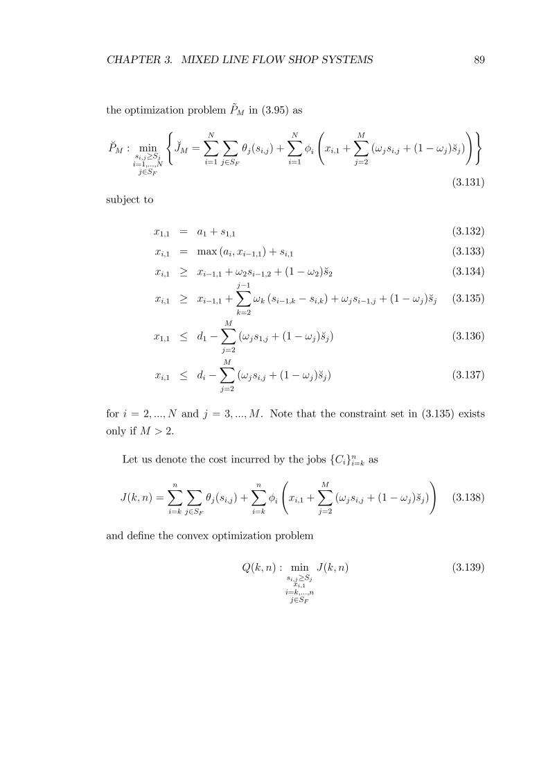
CHAPTER 3. MIXED LINE FLOW SHOP SYSTEMS 89
the optimization problem ~PM in (3.95) as
�PM : minsi;j�Sji=1;:::;Nj2SF
(�JM =
NXi=1
Xj2SF
�j(si;j) +
NXi=1
�i
xi;1 +
MXj=2
(!jsi;j + (1� !j)�sj)!)
(3.131)
subject to
x1;1 = a1 + s1;1 (3.132)
xi;1 = max (ai; xi�1;1) + si;1 (3.133)
xi;1 � xi�1;1 + !2si�1;2 + (1� !2)�s2 (3.134)
xi;1 � xi�1;1 +
j�1Xk=2
!k (si�1;k � si;k) + !jsi�1;j + (1� !j)�sj (3.135)
x1;1 � d1 �MXj=2
(!js1;j + (1� !j)�sj) (3.136)
xi;1 � di �MXj=2
(!jsi;j + (1� !j)�sj) (3.137)
for i = 2; :::; N and j = 3; :::;M . Note that the constraint set in (3.135) exists
only if M > 2.
Let us denote the cost incurred by the jobs fCigni=k as
J(k; n) =nXi=k
Xj2SF
�j(si;j) +nXi=k
�i
xi;1 +
MXj=2
(!jsi;j + (1� !j)�sj)!
(3.138)
and de�ne the convex optimization problem
Q(k; n) : minsi;j�Sjxi;1
i=k;:::;nj2SF
J(k; n) (3.139)
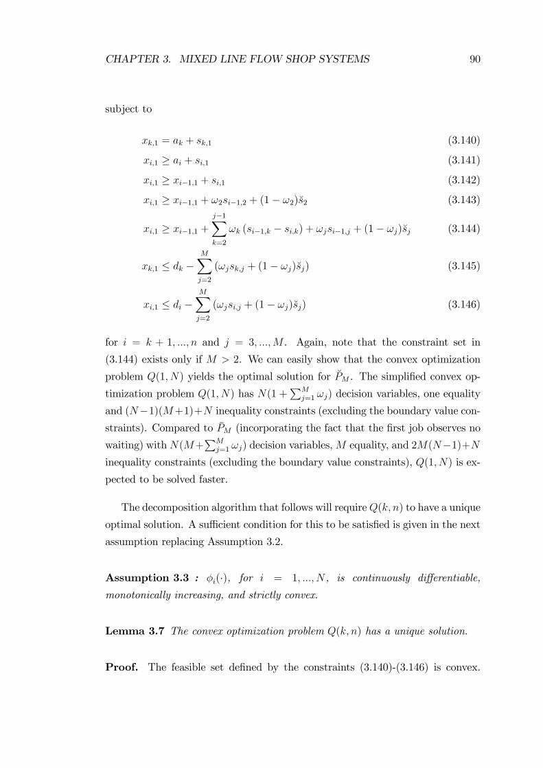
CHAPTER 3. MIXED LINE FLOW SHOP SYSTEMS 90
subject to
xk;1 = ak + sk;1 (3.140)
xi;1 � ai + si;1 (3.141)
xi;1 � xi�1;1 + si;1 (3.142)
xi;1 � xi�1;1 + !2si�1;2 + (1� !2)�s2 (3.143)
xi;1 � xi�1;1 +j�1Xk=2
!k (si�1;k � si;k) + !jsi�1;j + (1� !j)�sj (3.144)
xk;1 � dk �MXj=2
(!jsk;j + (1� !j)�sj) (3.145)
xi;1 � di �MXj=2
(!jsi;j + (1� !j)�sj) (3.146)
for i = k + 1; :::; n and j = 3; :::;M . Again, note that the constraint set in
(3.144) exists only if M > 2. We can easily show that the convex optimization
problem Q(1; N) yields the optimal solution for �PM . The simpli�ed convex op-
timization problem Q(1; N) has N(1 +PM
j=1 !j) decision variables, one equality
and (N�1)(M+1)+N inequality constraints (excluding the boundary value con-
straints). Compared to �PM (incorporating the fact that the �rst job observes no
waiting) withN(M+PM
j=1 !j) decision variables,M equality, and 2M(N�1)+Ninequality constraints (excluding the boundary value constraints), Q(1; N) is ex-
pected to be solved faster.
The decomposition algorithm that follows will requireQ(k; n) to have a unique
optimal solution. A su¢ cient condition for this to be satis�ed is given in the next
assumption replacing Assumption 3.2.
Assumption 3.3 : �i(�), for i = 1; :::; N , is continuously di¤erentiable,
monotonically increasing, and strictly convex.
Lemma 3.7 The convex optimization problem Q(k; n) has a unique solution.
Proof. The feasible set de�ned by the constraints (3.140)-(3.146) is convex.
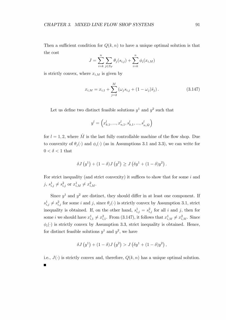
CHAPTER 3. MIXED LINE FLOW SHOP SYSTEMS 91
Then a su¢ cient condition for Q(k; n) to have a unique optimal solution is that
the cost
J =
nXi=k
Xj2SF
�j(si;j) +nXi=k
�i(xi;M)
is strictly convex, where xi;M is given by
xi;M = xi;1 +MXj=2
(!jsi;j + (1� !j)�sj) : (3.147)
Let us de�ne two distinct feasible solutions y1 and y2 such that
yl =�xlk;1; :::; x
ln;1; s
lk;1; :::; s
ln;M
�for l = 1; 2, where M is the last fully controllable machine of the �ow shop. Due
to convexity of �j(�) and �i(�) (as in Assumptions 3.1 and 3.3), we can write for0 < � < 1 that
�J�y1�+ (1� �)J
�y2�� J
��y1 + (1� �)y2
�:
For strict inequality (and strict convexity) it su¢ ces to show that for some i and
j, s1i;j 6= s2i;j or x1i;M 6= x2i;M .
Since y1 and y2 are distinct, they should di¤er in at least one component. If
s1i;j 6= s2i;j for some i and j, since �j(�) is strictly convex by Assumption 3.1, strictinequality is obtained. If, on the other hand, s1i;j = s
2i;j for all i and j, then for
some i we should have x1i;1 6= x2i;1. From (3.147), it follows that x1i;M 6= x2i;M . Since�i(�) is strictly convex by Assumption 3.3, strict inequality is obtained. Hence,for distinct feasible solutions y1 and y2, we have
�J�y1�+ (1� �)J
�y2�> J
��y1 + (1� �)y2
�;
i.e., J(�) is strictly convex and, therefore, Q(k; n) has a unique optimal solution.
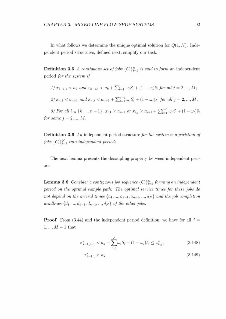
CHAPTER 3. MIXED LINE FLOW SHOP SYSTEMS 92
In what follows we determine the unique optimal solution for Q(1; N). Inde-
pendent period structures, de�ned next, simplify our task.
De�nition 3.5 A contiguous set of jobs fCigni=k is said to form an independent
period for the system if
1) xk�1;1 < ak and xk�1;j < ak +Pj�1
l=1 !lSl + (1� !l)�sl for all j = 2; :::;M ;
2) xn;1 < an+1 and xn;j < an+1 +Pj�1
l=1 !lSl + (1� !l)�sl for all j = 2; :::;M ;
3) For all i 2 fk; :::; n� 1g, xi;1 � ai+1 or xi;j � ai+1+Pj�1
l=1 !lSl+ (1�!l)�slfor some j = 2; :::;M .
De�nition 3.6 An independent period structure for the system is a partition of
jobs fCigNi=1 into independent periods.
The next lemma presents the decoupling property between independent peri-
ods.
Lemma 3.8 Consider a contiguous job sequence fCigni=k forming an independentperiod on the optimal sample path. The optimal service times for these jobs do
not depend on the arrival times fa1; :::; ak�1; an+1; :::; aNg and the job completiondeadlines fd1; :::; dk�1; dn+1; :::; dNg of the other jobs.
Proof. From (3.44) and the independent period de�nition, we have for all j =
1; :::;M � 1 that
x�k�1;j+1 < ak +
jXl=1
!lSl + (1� !l)�sl � x�k;j; (3.148)
x�k�1;1 < ak (3.149)
CHAPTER 3. MIXED LINE FLOW SHOP SYSTEMS 93
for k > 1 and
x�n;j+1 < an+1 +
jXl=1
!lSl + (1� !l)�sl � x�n+1;j; (3.150)
x�n;1 < an+1 (3.151)
for n < N . Note that the optimal departures satis�es (3.2)-(3.5); therefore from
(3.42), (3.49), (3.55), (3.150), and (3.151), we have for j = 1; :::;M � 1
��n;j + ��n;j = �
�n+1;j + �
�n;j+1 = �
�n;j+1
and
��n;M + ��n;M = �0n(x
�n;M) + �
�n+1;M +
�n = �
0n(x
�n;M) +
�n:
Hence, there is no dependence of ��n;j for j = 1; :::;M to jobs fCn+1; :::; CNg, i.e.,the information is not propagated in the backward direction between independent
periods. Note that if n = N then there is no need for checking the backward
information propagation.
Similarly, let us employ inequalities (3.148) and (3.149) in (3.2) and (3.3) to
observe that
x�k;j = max�x�k;j�1; x
�k�1;j
�+ !js
�k;j + (1� !j)�sj
= x�k;j�1 + !js�k;j + (1� !j)�sj:
Hence, there is no dependence of x�k;j for j = 1; :::;M to jobs fC1; :::; Ck�1g, i.e.,the information is not propagated in the forward direction between independent
periods. Note that if k = 1 then there is no need for checking the forward
information propagation.
Hence, independent periods are decoupled from each other.
Let us assume that the optimal independent period structure is given. Let B
be the number of independent periods in this structure, and let Ck(b) and Cn(b)denote the �rst and the last jobs of the bth independent period where b = 1; :::; B.
CHAPTER 3. MIXED LINE FLOW SHOP SYSTEMS 94
We can rewrite �PM as
�PM : minsi;j�Sji=1;:::;Nj2SF
(J =
BXb=1
J (k(b); n(b))
)
subject to (3.132)-(3.137). By the independent period de�nition, the constraints
(3.133)-(3.135) for i = k(b) can be reduced to xk(b);1 = ak(b) + sk(b);1 which is
satis�ed by the optimal solution. Along with the decoupling property shown in
Lemma 3.8, this allows for the decomposition of �PM into B smaller optimization
problems P (k(b); n(b)) de�ned as
P (k(b); n(b)) : minsi;j�Sj
i=k(b);:::;n(b)j2SF
J (k(b); n(b))
subject to
xk(b);1 = ak(b) + sk(b);1
xi;1 = max (ai; xi�1;1) + si;1
xi;1 � xi�1;1 + !2si�1;2 + (1� !2)�s2
xi;1 � xi�1;1 +j�1Xk=2
!k (si�1;k � si;k) + !jsi�1;j + (1� !j)�sj
xk(b);1 � dk(b) �MXj=2
�!jsk(b);j + (1� !j)�sj
�xi;1 � di �
MXj=2
(!jsi;j + (1� !j)�sj)
for i = k(b) + 1; :::; n(b) and j = 3; :::;M . Note that, similarly, Q(k(b); n(b)) can
easily be shown to have the same optimal solution as that of P (k(b); n(b)).
We denote the optimal solution of Q(k; n) as s�i;j(k; n) and x�i;1(k; n), and the
corresponding departure times as x�i;j(k; n) for i = k; :::; n and j = 1; :::;M . The
following corollary follows from Lemma 3.8 and relates the optimal solution of
Q(k; n) to the optimal solution of PM .
CHAPTER 3. MIXED LINE FLOW SHOP SYSTEMS 95
Corollary 3.1 If the job sequence fCigni=k forms an independent period on theoptimal sample path, then the optimal solution of Q(k; n) satis�es
s�i;j(k; n) = s�i;j;
x�i;1(k; n) = x�i;1
for i = k; :::; n and j = 1; :::;M .
This corollary forms the basis for our decomposition algorithm.
So far we have shown that if the optimal independent period structure can
be identi�ed, Q(1; N) can be decomposed into a set of smaller problems. The
following lemma provides necessary and su¢ cient conditions for identifying the
independent periods on the optimal sample path based on the solution of Q(k; n).
Lemma 3.9 Let Ck initiate an independent period on the optimal sample path.
The job Cn (k � n) ends the independent period if and only if the following
conditions are satis�ed:
1. x�n;1(k; n) < an+1 and x�n;j(k; n) < an+1 +Pj�1
l=1 !lSl + (1 � !l)�sl for allj = 2; :::;M ;
2. For all i 2 fk; :::; n�1g, x�i;1(k; n) � ai+1 or x�i;j(k; n) � ai+1+Pj�1
l=1 !lSl+
(1� !l)�sl for some j = 2; :::;M .
Proof. (Necessity) Since jobs fCigni=k form an independent period on the optimalsample path, and since x�i;j(k; n) = x
�i;j by Corollary 3.1, the result follows from
the independent period de�nition.
(Su¢ ciency) Assume that even though both conditions are satis�ed, Cn does
not end the independent period, i.e., for some n0 > n, jobs fCign0i=k form an
independent period on the optimal sample path.
CHAPTER 3. MIXED LINE FLOW SHOP SYSTEMS 96
Let us de�ne a solution for Q(k; n0) as
si;j =
8>><>>:s�i;j(k; n); i 2 fk; :::; ng and j 2 SF
s�i;j(k; n0) + � ; i = n+ 1; j = 1
s�i;j(k; n0); otherwise
(3.152)
and
xi;1 =
(x�i;1(k; n); i 2 fk; :::; ngx�i;1(k; n
0); i 2 fn+ 1; :::; n0g;(3.153)
where � � 0 is de�ned as
� = max�x�n;1(k; n
0)� an+1; 0�:
By the independent period de�nition, since Cn is not the last job of the inde-
pendent period, x�n;1(k; n0) � an+1 or x�n;j(k; n0) � an+1 +
Pj�1l=1 !lSl + (1 � !l)�sl
for some j = 2; :::;M . It follows from the �rst condition that
s�i;j(k; n) 6= s�i;j(k; n0) (3.154)
or
x�i;1(k; n) 6= x�i;1(k; n0) (3.155)
for some i = k; :::; n and j = 1; :::;M . Therefore, by Lemma 3.7, the solution
given in (3.152) and (3.153) is not optimal for Q(k; n0).
Let us check the feasibility of this non-optimal solution: Since si;j and xi;1 for
i = k; :::; n and j 2 SF are the solutions for the problem Q(k; n), they satisfy theconstraints (3.140)-(3.146) for i = k+ 1; :::; n and j = 3; :::;M . For i = n+ 1, we
CHAPTER 3. MIXED LINE FLOW SHOP SYSTEMS 97
have
xn+1;1 = x�n+1;1(k; n
0)
= max�x�n;1(k; n
0); an+1�+ s�n+1;1(k; n
0)
= an+1 + � + s�n+1;1(k; n
0)
= an+1 + sn+1;1
= max (an+1; xn;1) + sn+1;1
satisfying the constraints (3.141), (3.142), and (3.146). It follows from the �rst
condition and from sn+1;j � Sj for all j 2 SF that the constraints (3.143) and(3.144) are also satis�ed for i = n+1. Finally, since si;j and xi;1 for i = n+2; :::; n0
and j 2 SF are the solutions for Q(k; n0), the constraints (3.141)-(3.144), and(3.146) are satis�ed for i = n+2; :::; n0 and j = 3; :::;M . Hence, the non-optimal
solution is feasible for the Q(k; n0) problem.
Let us recall from Corollary 3.1 that
s�i;j = s�i;j(k; n
0);
x�i;1 = x�i;1(k; n
0)
for i = k; :::; n0 and j 2 SF , and consider the problem Q(k; n0). Its optimal cost
can be written as
J�(k; n0) = J�A(k; n0) + J�B(k; n
0); (3.156)
where
J�A(k; n0) =
nXi=k
Xj2SF
�j(s�i;j) +
nXi=k
�i
x�i;1 +
MXj=2
(!js�i;j + (1� !j)�sj)
!
and
J�B(k; n0) =
n0Xi=n+1
Xj2SF
�j(s�i;j) +
n0Xi=n+1
�i
x�i;1 +
MXj=2
(!js�i;j + (1� !j)�sj)
!:
The cost J(k; n0) due to applying the non-optimal solution in (3.152) and (3.153)
CHAPTER 3. MIXED LINE FLOW SHOP SYSTEMS 98
can be written as
J(k; n0) = J�(k; n) + JC ; (3.157)
where
JC = J�B(k; n
0) + �1�s�n+1;1(k; n
0) + ��� �1
�s�n+1;1(k; n
0)�:
Since the optimal solution of Q(k; n) is unique by Lemma 3.7, from (3.154) and
(3.155),
J�A(k; n0) > J�(k; n): (3.158)
Moreover, due to Assumption 3.1,
J�B(k; n0) � JC ; (3.159)
which also accounts for the case that � = 0. From (3.156), (3.157), (3.158), and
(3.159),
J�(k; n0) > J(k; n0);
in other words, the cost of the non-optimal solution is lower than the optimal
cost, which is a contradiction. Hence, the result follows.
Lemma 3.9 allows us to identify independent periods on the optimal sample
path. If Ck is the �rst job of an independent period, we can identify this inde-
pendent period by sequentially solving Q(k; n) and checking for all jobs fCigni=kto see if both conditions in Lemma 3.9 are satis�ed.
The next lemma indicates that checking only for job Cn to see if the �rst
condition in Lemma 3.9 is satis�ed su¢ ces to identify the independent period.
Lemma 3.10 Let Ck initiate an independent period on the optimal sample path.
For all i � k, if x�i;1(k; i) � ai+1 or x�i;j(k; i) � ai+1 +Pj�1
l=1 !lSl + (1 � !l)�sl forsome j = 2; :::;M , then for all n � i, x�i;1(k; n) � ai+1 or x�i;j(k; n) � ai+1 +Pj�1
l=1 !lSl + (1� !l)�sl for some j = 2; :::;M .
Proof. (By contradiction) Let us assume that there exists n > i such that
x�i;1(k; n) < ai+1 and x�i;j(k; n) < ai+1+
Pj�1l=1 !lSl+(1�!l)�sl for all j = 2; :::;M .
CHAPTER 3. MIXED LINE FLOW SHOP SYSTEMS 99
In that case job Ci ends an independent period (not necessarily the one that was
started by job Ck). From the decoupling property in Lemma 3.8 and Corollary
3.1, we should have
x�i;j(k; i) = x�i;j(k; n):
However, since x�i;1(k; i) � ai+1 or x�i;j(k; i) � ai+1 +Pj�1
l=1 !lSl + (1 � !l)�sl forsome j = 2; :::;M , a contradiction is observed. Hence the result follows.
Lemma 3.10 asserts that an independent period formed by jobs fCigni=k isidenti�ed as soon as the problem Q(k; n) is solved. This result is formalized in
the following theorem.
Theorem 3.2 Jobs fCigni=k form an independent period on the optimal sample
path if and only if the following conditions are satis�ed:
1) x�k�1;1 < ak and x�k�1;j < ak +
Pj�1l=1 !lSl + (1� !l)�sl for all j = 2; :::;M ;
2) For all i 2 fk; :::; n� 1g, x�i;1(k; i) � ai+1 or x�i;j(k; i) � ai+1+Pj�1
l=1 !lSl+
(1� !l)�sl for some j = 2; :::;M ;
3) x�n;1(k; n) < an+1 and x�n;j(k; n) < an+1 +Pj�1
l=1 !lSl + (1 � !l)�sl for allj = 2; :::;M .
Proof. It follows from Lemma 3.9, Lemma 3.10, and the independent period
de�nition.
Our forward decomposition algorithm is based on Theorem 3.2. While iden-
tifying the optimal independent period structure, this algorithm also determines
the optimal solution.
Algorithm 3.1 Step 1: (initialization) k = 1; n = 1; aN+1 =1:
while n � N do
Step 2: Solve subproblem Q(k; n):
CHAPTER 3. MIXED LINE FLOW SHOP SYSTEMS 100
Step 3: (identify independent periods)
If x�n;1(k; n) < an+1 and x�n;j(k; n) < an+1 +
Pj�1l=1 !lSl + (1 � !l)�sl
for all j = 2 to M , then
s�i;j = s�i;j(k; n) for i = k; :::; n and j 2 SF ;
k = n+ 1;
endif.
Step 4: (increment index n)
n = n+ 1:
Note that this decomposition algorithm requires only N iterations. However,
these iterations are not identical in complexity and depend on the arrival sequence
along with the cost parameters. The best case for this algorithm would be an
optimal sample path where each job forms an independent period of its own. In
this case, Q(i; i) for all i = 1; :::; N are solved. The worst case for this algorithm,
on the other hand, would be an optimal sample path where all jobs reside in the
same independent period and no decomposition is observed. In the worst case, we
solve Q(1; i) for all i = 1; :::; N . If the number of independent periods expected
is low, e.g. for the bulk arrivals case we have only one independent period, we
may choose to solve Q(1; N) directly.
3.5 Numerical Study
Let us consider an M -machine �ow shop system processing an identical set of N
jobs. The service cost �j(s) for job Ci at the fully controllable machine j is given
as
�j(si;j) =�jsi;j; (3.160)
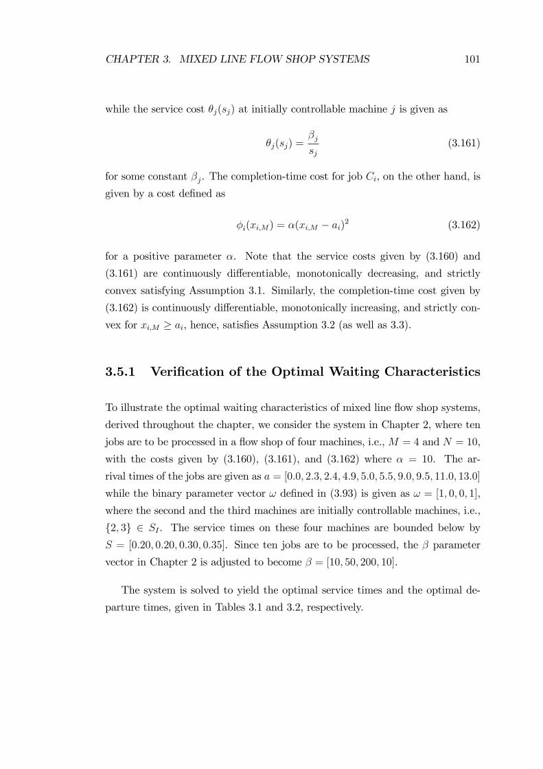
CHAPTER 3. MIXED LINE FLOW SHOP SYSTEMS 101
while the service cost �j(sj) at initially controllable machine j is given as
�j(sj) =�jsj
(3.161)
for some constant �j. The completion-time cost for job Ci, on the other hand, is
given by a cost de�ned as
�i(xi;M) = �(xi;M � ai)2 (3.162)
for a positive parameter �. Note that the service costs given by (3.160) and
(3.161) are continuously di¤erentiable, monotonically decreasing, and strictly
convex satisfying Assumption 3.1. Similarly, the completion-time cost given by
(3.162) is continuously di¤erentiable, monotonically increasing, and strictly con-
vex for xi;M � ai, hence, satis�es Assumption 3.2 (as well as 3.3).
3.5.1 Veri�cation of the Optimal Waiting Characteristics
To illustrate the optimal waiting characteristics of mixed line �ow shop systems,
derived throughout the chapter, we consider the system in Chapter 2, where ten
jobs are to be processed in a �ow shop of four machines, i.e., M = 4 and N = 10,
with the costs given by (3.160), (3.161), and (3.162) where � = 10. The ar-
rival times of the jobs are given as a = [0:0; 2:3; 2:4; 4:9; 5:0; 5:5; 9:0; 9:5; 11:0; 13:0]
while the binary parameter vector ! de�ned in (3.93) is given as ! = [1; 0; 0; 1],
where the second and the third machines are initially controllable machines, i.e.,
f2; 3g 2 SI . The service times on these four machines are bounded below by
S = [0:20; 0:20; 0:30; 0:35]. Since ten jobs are to be processed, the � parameter
vector in Chapter 2 is adjusted to become � = [10; 50; 200; 10].
The system is solved to yield the optimal service times and the optimal de-
parture times, given in Tables 3.1 and 3.2, respectively.
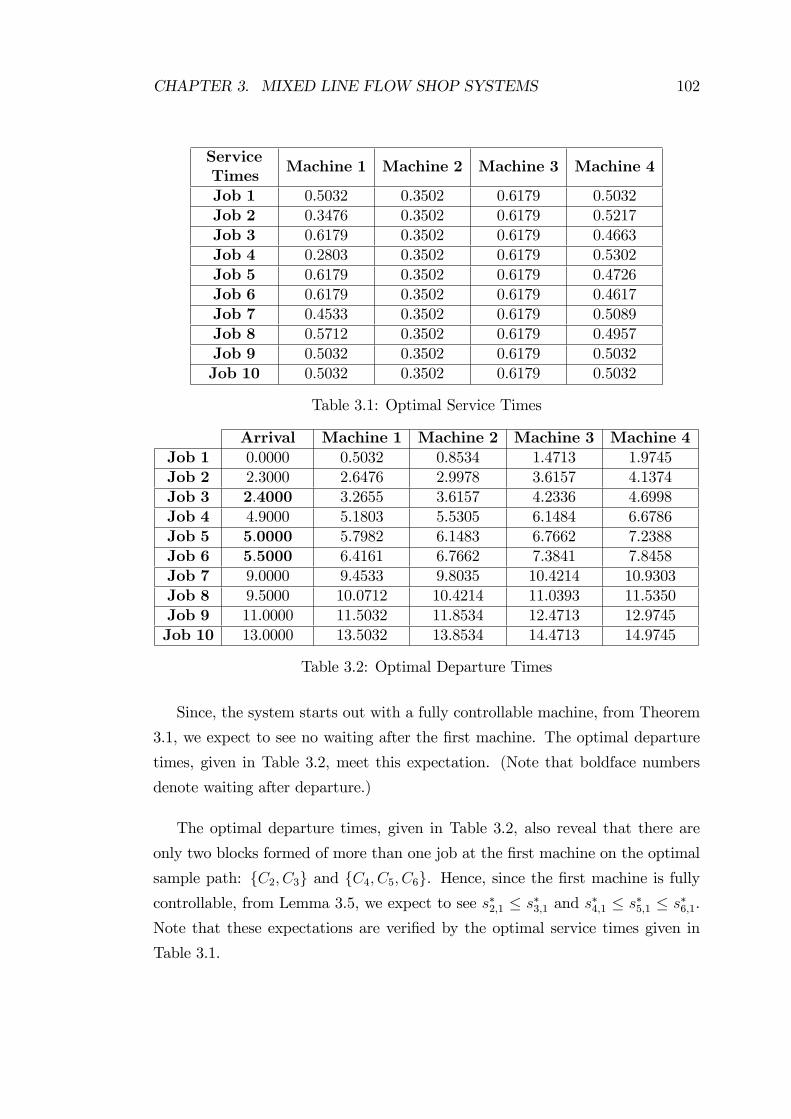
CHAPTER 3. MIXED LINE FLOW SHOP SYSTEMS 102
ServiceTimes
Machine 1 Machine 2 Machine 3 Machine 4
Job 1 0.5032 0.3502 0.6179 0.5032Job 2 0.3476 0.3502 0.6179 0.5217Job 3 0.6179 0.3502 0.6179 0.4663Job 4 0.2803 0.3502 0.6179 0.5302Job 5 0.6179 0.3502 0.6179 0.4726Job 6 0.6179 0.3502 0.6179 0.4617Job 7 0.4533 0.3502 0.6179 0.5089Job 8 0.5712 0.3502 0.6179 0.4957Job 9 0.5032 0.3502 0.6179 0.5032Job 10 0.5032 0.3502 0.6179 0.5032
Table 3.1: Optimal Service Times
Arrival Machine 1 Machine 2 Machine 3 Machine 4Job 1 0.0000 0.5032 0.8534 1.4713 1.9745Job 2 2.3000 2.6476 2.9978 3.6157 4.1374Job 3 2:4000 3.2655 3.6157 4.2336 4.6998Job 4 4.9000 5.1803 5.5305 6.1484 6.6786Job 5 5:0000 5.7982 6.1483 6.7662 7.2388Job 6 5:5000 6.4161 6.7662 7.3841 7.8458Job 7 9.0000 9.4533 9.8035 10.4214 10.9303Job 8 9.5000 10.0712 10.4214 11.0393 11.5350Job 9 11.0000 11.5032 11.8534 12.4713 12.9745Job 10 13.0000 13.5032 13.8534 14.4713 14.9745
Table 3.2: Optimal Departure Times
Since, the system starts out with a fully controllable machine, from Theorem
3.1, we expect to see no waiting after the �rst machine. The optimal departure
times, given in Table 3.2, meet this expectation. (Note that boldface numbers
denote waiting after departure.)
The optimal departure times, given in Table 3.2, also reveal that there are
only two blocks formed of more than one job at the �rst machine on the optimal
sample path: fC2; C3g and fC4; C5; C6g. Hence, since the �rst machine is fullycontrollable, from Lemma 3.5, we expect to see s�2;1 � s�3;1 and s�4;1 � s�5;1 � s�6;1.Note that these expectations are veri�ed by the optimal service times given in
Table 3.1.
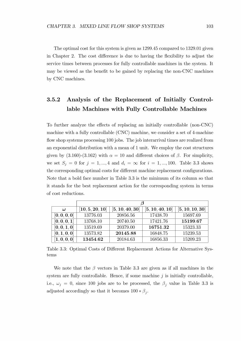
CHAPTER 3. MIXED LINE FLOW SHOP SYSTEMS 103
The optimal cost for this system is given as 1299:45 compared to 1329:01 given
in Chapter 2. The cost di¤erence is due to having the �exibility to adjust the
service times between processes for fully controllable machines in the system. It
may be viewed as the bene�t to be gained by replacing the non-CNC machines
by CNC machines.
3.5.2 Analysis of the Replacement of Initially Control-
lable Machines with Fully Controllable Machines
To further analyze the e¤ects of replacing an initially controllable (non-CNC)
machine with a fully controllable (CNC) machine, we consider a set of 4-machine
�ow shop systems processing 100 jobs. The job interarrival times are realized from
an exponential distribution with a mean of 1 unit. We employ the cost structures
given by (3.160)-(3.162) with � = 10 and di¤erent choices of �. For simplicity,
we set Sj = 0 for j = 1; :::; 4 and di = 1 for i = 1; :::; 100. Table 3.3 shows
the corresponding optimal costs for di¤erent machine replacement con�gurations.
Note that a bold face number in Table 3.3 is the minimum of its column so that
it stands for the best replacement action for the corresponding system in terms
of cost reductions.
�! [10;5;20;10] [5;10;40;30] [5;10;40;10] [5;10;10;30]
[0;0;0;0] 13776.03 20856.56 17438.70 15697.69[0;0;0;1] 13768.10 20740.50 17421.76 15199:67[0;0;1;0] 13519.69 20379.00 16751:32 15323.33[0;1;0;0] 13573.82 20145:88 16848.75 15239.53[1;0;0;0] 13454:62 20184.63 16856.33 15209.23
Table 3.3: Optimal Costs of Di¤erent Replacement Actions for Alternative Sys-tems
We note that the � vectors in Table 3.3 are given as if all machines in the
system are fully controllable. Hence, if some machine j is initially controllable,
i.e., !j = 0, since 100 jobs are to be processed, the �j value in Table 3.3 is
adjusted accordingly so that it becomes 100 � �j.
CHAPTER 3. MIXED LINE FLOW SHOP SYSTEMS 104
Due having �exibility to adjust the service times between processes for a
fully controllable machine, we expect cost reductions by replacing an initially
controllable machine with its fully controllable counterpart. Table 3.3 meets this
expectation: independent of its location and �j value, replacement action of any
initially controllable machine j always reduces the cost. The second question for
which we look an answer is the choice of the initially controllable machine to be
replaced for the highest cost reduction. Table 3.3 reveals that the location of the
initially controllable machine to be replaced for the highest cost reduction relies
on the machine con�gurations in the system: replacement of initially controllable
machines with four di¤erent locations turned out to be the best policy in terms of
cost reductions for four di¤erent system con�gurations. Hence, there is no simple
rule for the best replacement policy in terms of cost reductions.
3.5.3 Analysis of the E¤ects of the Locations of Fully Con-
trollable Machines
To analyze the e¤ects of the locations of fully controllable machines in the sys-
tem, we consider a 3-machine �ow shop system processing 100 jobs. The job
interarrival times are realized from an exponential distribution with a mean of
1 unit and the cost functions in (3.160)-(3.162) with � = 10 and � = [5; 10; 20]
are used. However, we should note that, for some initially controllable machine
j, we adjust its �j value accordingly so that it becomes 100 � �j. Finally, we setSj = 0 for j = 1; :::; 4 and di =1 for i = 1; :::; 100. Tables 3.4 and 3.5 represent
the optimal costs for each possible layout con�guration with at least one fully
controllable and one initially controllable machine for this system. We note that
��j indicates that machine j is fully controllable and the optimal cost of the cost
minimizing layout con�guration for the corresponding system is represented by a
bold face character in these tables.
When we examine the optimization problems ~PM in (3.95) and PM in (3.111)
presented in Section 3.3, a change in the order of the initially controllable ma-
chines within an initially controllable portion does not change the overall problem.
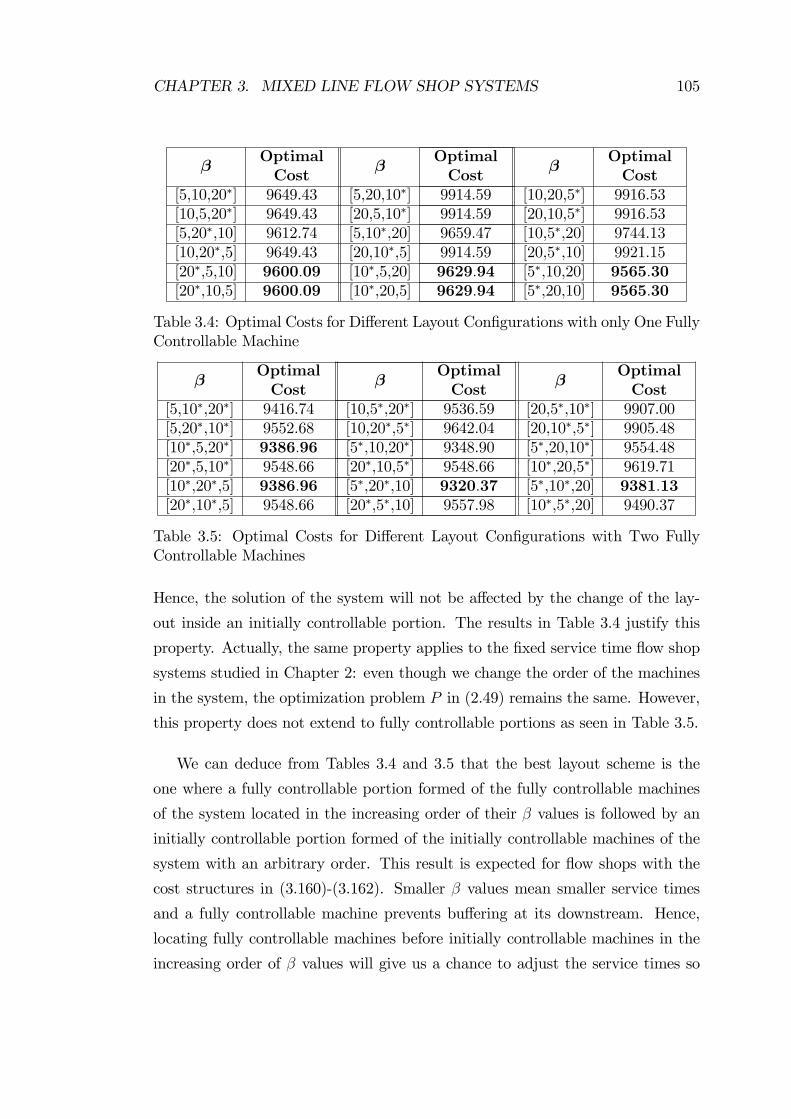
CHAPTER 3. MIXED LINE FLOW SHOP SYSTEMS 105
�OptimalCost
�OptimalCost
�OptimalCost
[5,10,20�] 9649.43 [5,20,10�] 9914.59 [10,20,5�] 9916.53[10,5,20�] 9649.43 [20,5,10�] 9914.59 [20,10,5�] 9916.53[5,20�,10] 9612.74 [5,10�,20] 9659.47 [10,5�,20] 9744.13[10,20�,5] 9649.43 [20,10�,5] 9914.59 [20,5�,10] 9921.15[20�,5,10] 9600:09 [10�,5,20] 9629:94 [5�,10,20] 9565:30[20�,10,5] 9600:09 [10�,20,5] 9629:94 [5�,20,10] 9565:30
Table 3.4: Optimal Costs for Di¤erent Layout Con�gurations with only One FullyControllable Machine
�OptimalCost
�OptimalCost
�OptimalCost
[5,10�,20�] 9416.74 [10,5�,20�] 9536.59 [20,5�,10�] 9907.00[5,20�,10�] 9552.68 [10,20�,5�] 9642.04 [20,10�,5�] 9905.48[10�,5,20�] 9386:96 [5�,10,20�] 9348.90 [5�,20,10�] 9554.48[20�,5,10�] 9548.66 [20�,10,5�] 9548.66 [10�,20,5�] 9619.71[10�,20�,5] 9386:96 [5�,20�,10] 9320:37 [5�,10�,20] 9381:13[20�,10�,5] 9548.66 [20�,5�,10] 9557.98 [10�,5�,20] 9490.37
Table 3.5: Optimal Costs for Di¤erent Layout Con�gurations with Two FullyControllable Machines
Hence, the solution of the system will not be a¤ected by the change of the lay-
out inside an initially controllable portion. The results in Table 3.4 justify this
property. Actually, the same property applies to the �xed service time �ow shop
systems studied in Chapter 2: even though we change the order of the machines
in the system, the optimization problem P in (2.49) remains the same. However,
this property does not extend to fully controllable portions as seen in Table 3.5.
We can deduce from Tables 3.4 and 3.5 that the best layout scheme is the
one where a fully controllable portion formed of the fully controllable machines
of the system located in the increasing order of their � values is followed by an
initially controllable portion formed of the initially controllable machines of the
system with an arbitrary order. This result is expected for �ow shops with the
cost structures in (3.160)-(3.162). Smaller � values mean smaller service times
and a fully controllable machine prevents bu¤ering at its downstream. Hence,
locating fully controllable machines before initially controllable machines in the
increasing order of � values will give us a chance to adjust the service times so
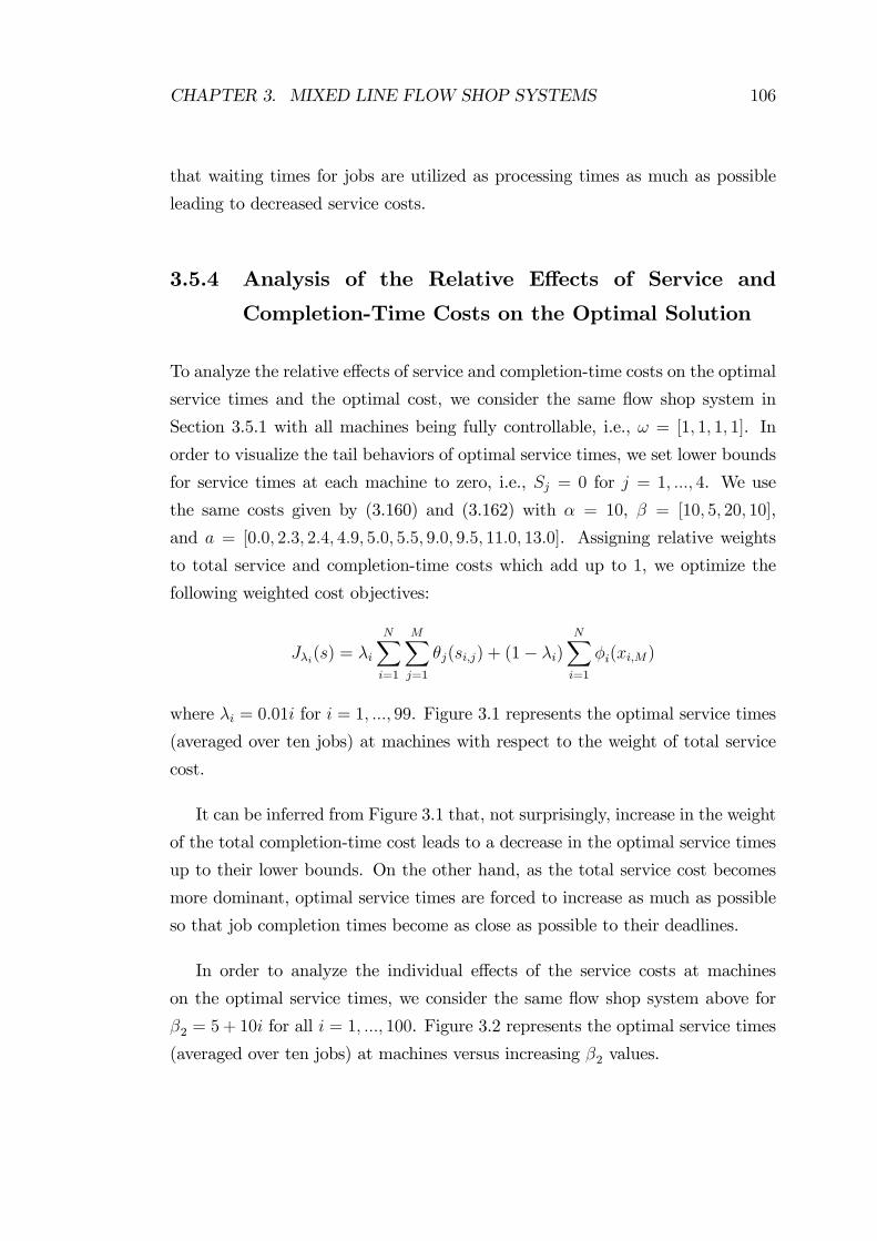
CHAPTER 3. MIXED LINE FLOW SHOP SYSTEMS 106
that waiting times for jobs are utilized as processing times as much as possible
leading to decreased service costs.
3.5.4 Analysis of the Relative E¤ects of Service and
Completion-Time Costs on the Optimal Solution
To analyze the relative e¤ects of service and completion-time costs on the optimal
service times and the optimal cost, we consider the same �ow shop system in
Section 3.5.1 with all machines being fully controllable, i.e., ! = [1; 1; 1; 1]. In
order to visualize the tail behaviors of optimal service times, we set lower bounds
for service times at each machine to zero, i.e., Sj = 0 for j = 1; :::; 4. We use
the same costs given by (3.160) and (3.162) with � = 10, � = [10; 5; 20; 10],
and a = [0:0; 2:3; 2:4; 4:9; 5:0; 5:5; 9:0; 9:5; 11:0; 13:0]. Assigning relative weights
to total service and completion-time costs which add up to 1, we optimize the
following weighted cost objectives:
J�i(s) = �i
NXi=1
MXj=1
�j(si;j) + (1� �i)NXi=1
�i(xi;M)
where �i = 0:01i for i = 1; :::; 99. Figure 3.1 represents the optimal service times
(averaged over ten jobs) at machines with respect to the weight of total service
cost.
It can be inferred from Figure 3.1 that, not surprisingly, increase in the weight
of the total completion-time cost leads to a decrease in the optimal service times
up to their lower bounds. On the other hand, as the total service cost becomes
more dominant, optimal service times are forced to increase as much as possible
so that job completion times become as close as possible to their deadlines.
In order to analyze the individual e¤ects of the service costs at machines
on the optimal service times, we consider the same �ow shop system above for
�2 = 5+ 10i for all i = 1; :::; 100. Figure 3.2 represents the optimal service times
(averaged over ten jobs) at machines versus increasing �2 values.
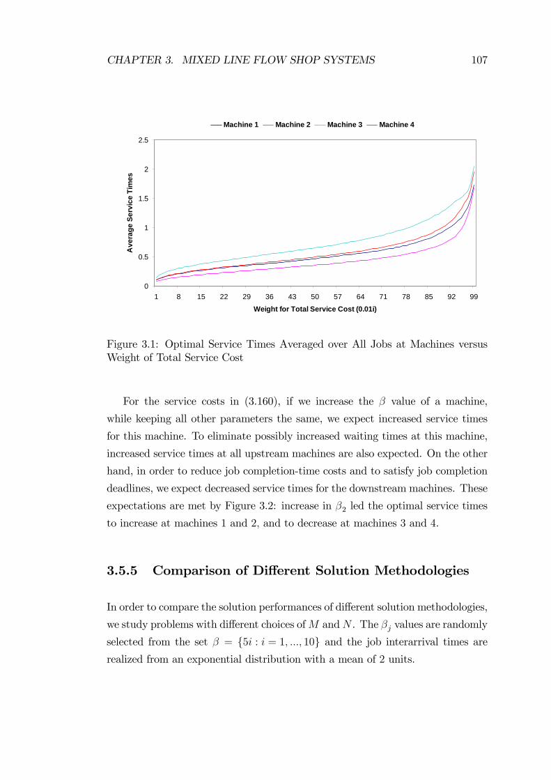
CHAPTER 3. MIXED LINE FLOW SHOP SYSTEMS 107
0
0.5
1
1.5
2
2.5
1 8 15 22 29 36 43 50 57 64 71 78 85 92 99
Weight for Total Service Cost (0.01i)
Ave
rage
Ser
vice
Tim
esMachine 1 Machine 2 Machine 3 Machine 4
Figure 3.1: Optimal Service Times Averaged over All Jobs at Machines versusWeight of Total Service Cost
For the service costs in (3.160), if we increase the � value of a machine,
while keeping all other parameters the same, we expect increased service times
for this machine. To eliminate possibly increased waiting times at this machine,
increased service times at all upstream machines are also expected. On the other
hand, in order to reduce job completion-time costs and to satisfy job completion
deadlines, we expect decreased service times for the downstream machines. These
expectations are met by Figure 3.2: increase in �2 led the optimal service times
to increase at machines 1 and 2; and to decrease at machines 3 and 4.
3.5.5 Comparison of Di¤erent Solution Methodologies
In order to compare the solution performances of di¤erent solution methodologies,
we study problems with di¤erent choices ofM andN . The �j values are randomly
selected from the set � = f5i : i = 1; :::; 10g and the job interarrival times arerealized from an exponential distribution with a mean of 2 units.
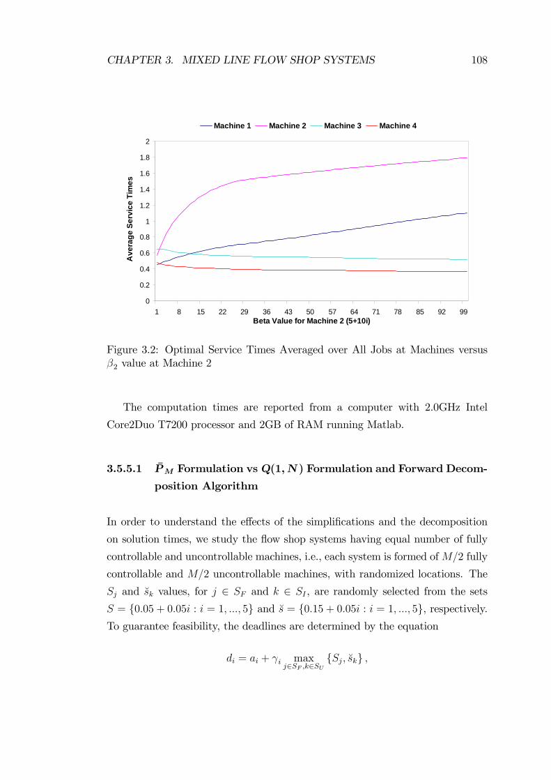
CHAPTER 3. MIXED LINE FLOW SHOP SYSTEMS 108
0
0.2
0.4
0.6
0.8
1
1.2
1.4
1.6
1.8
2
1 8 15 22 29 36 43 50 57 64 71 78 85 92 99Beta Value for Machine 2 (5+10i)
Ave
rage
Ser
vice
Tim
esMachine 1 Machine 2 Machine 3 Machine 4
Figure 3.2: Optimal Service Times Averaged over All Jobs at Machines versus�2 value at Machine 2
The computation times are reported from a computer with 2.0GHz Intel
Core2Duo T7200 processor and 2GB of RAM running Matlab.
3.5.5.1 �PM Formulation vsQ(1; N) Formulation and Forward Decom-
position Algorithm
In order to understand the e¤ects of the simpli�cations and the decomposition
on solution times, we study the �ow shop systems having equal number of fully
controllable and uncontrollable machines, i.e., each system is formed ofM=2 fully
controllable and M=2 uncontrollable machines, with randomized locations. The
Sj and �sk values, for j 2 SF and k 2 SI , are randomly selected from the sets
S = f0:05 + 0:05i : i = 1; :::; 5g and �s = f0:15 + 0:05i : i = 1; :::; 5g, respectively.To guarantee feasibility, the deadlines are determined by the equation
di = ai + i maxj2SF ;k2SU
fSj; �skg ;
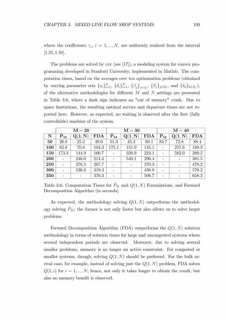
CHAPTER 3. MIXED LINE FLOW SHOP SYSTEMS 109
where the coe¢ cients i, i = 1; :::; N , are uniformly realized from the interval
[1:25; 1:50].
The problems are solved by cvx (see [17]), a modeling system for convex pro-
gramming developed in Stanford University, implemented in Matlab. The com-
putation times, based on the averages over ten optimization problems (obtained
by varying parameter sets faigNi=1, fdigNi=1, f�jgj2SF , fSjgj2SF , and f�skgk2SU ),of the alternative methodologies for di¤erent M and N settings are presented
in Table 3.6, where a dash sign indicates an "out of memory" crash. Due to
space limitations, the resulting optimal service and departure times are not re-
ported here. However, as expected, no waiting is observed after the �rst (fully
controllable) machine of the system.
M = 20 M = 30 M = 40N �PM Q(1;N) FDA �PM Q(1;N) FDA �PM Q(1;N) FDA50 26.8 25.2 49.0 51.3 45.3 68.1 83.7 72.8 88.4100 82.8 70.8 104.3 175.1 151.0 145.1 - 257.6 188.3150 173.3 144.9 160.7 - 328.9 224.1 - 582.0 289.2200 - 246.0 214.4 - 540.1 296.4 - - 381.5250 - 376.5 267.7 - - 370.3 - - 478.2300 - 536.6 319.3 - - 438.9 - - 570.2350 - - 370.3 - - 506.7 - - 658.3
Table 3.6: Computation Times for �PM and Q(1; N) Formulations, and ForwardDecomposition Algorithm (in seconds)
As expected, the methodology solving Q(1; N) outperforms the methodol-
ogy solving �PM ; the former is not only faster but also allows us to solve larger
problems.
Forward Decomposition Algorithm (FDA) outperforms the Q(1; N) solution
methodology in terms of solution times for large and uncongested systems where
several independent periods are observed. Moreover, due to solving several
smaller problems, memory is no longer an active constraint. For congested or
smaller systems, though, solving Q(1; N) should be preferred. For the bulk ar-
rival case, for example, instead of solving just the Q(1; N) problem, FDA solves
Q(1; i) for i = 1; :::; N ; hence, not only it takes longer to obtain the result, but
also no memory bene�t is observed.
CHAPTER 3. MIXED LINE FLOW SHOP SYSTEMS 110
3.5.5.2 Forward Decomposition Algorithm vs Virtual Deadline Algo-
rithm
We also compare the solution performance of Forward Decomposition Algorithm
(FDA) with recently developed Virtual Deadline Algorithm (VDA) by Mao and
Cassandras [31]. The main idea of this algorithm is to introduce virtual deadlines
at each machine except the last one so that the M -machine problem is replaced
by M single machine problems which can be solved very e¤ectively by existing
solution methodologies such as Critical Task Decomposition Algorithm (CTDA)
developed in [32]. However, determination of the appropriate virtual deadlines for
each machine requires the solution of additional N+M�1 simpleM -dimensionalconvex optimization problems. The sequence of solutions to simple single machine
problems with virtual deadlines updated through solving these M -dimensional
convex optimization problems at each step was shown to converge to the global
optimal solution of the original problem.
In particular, VDA is a solution procedure for �ow shop systems consisting
only of fully controllable machines where the job completion-time costs are not
included. To notice that, in our model, we may also have uncontrollable machines
in the system and we include job completion-time costs in the objective function.
However, VDA is also applicable for non-homogeneous service cost structures,
i.e., the service cost functions may be di¤erent both for each machine and each
job, while we assign the same service cost functions to all jobs at fully control-
lable machines, i.e., homogeneous service costs for all jobs at fully controllable
machines.
We study the �ow shop systems consisting only of fully controllable machines
by removing the job completion-time costs from the objective function so that
VDA becomes applicable. The deadlines are determined by the equation
di = ai +M � i;
where the coe¢ cients i, i = 1; :::; N , are uniformly realized from the interval
[0:25; 0:30]. We note that feasibility is guaranteed by these deadlines. Since the
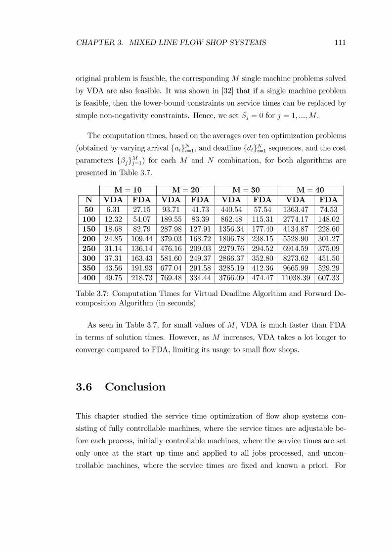
CHAPTER 3. MIXED LINE FLOW SHOP SYSTEMS 111
original problem is feasible, the correspondingM single machine problems solved
by VDA are also feasible. It was shown in [32] that if a single machine problem
is feasible, then the lower-bound constraints on service times can be replaced by
simple non-negativity constraints. Hence, we set Sj = 0 for j = 1; :::;M .
The computation times, based on the averages over ten optimization problems
(obtained by varying arrival faigNi=1, and deadline fdigNi=1 sequences, and the costparameters f�jgMj=1) for each M and N combination, for both algorithms are
presented in Table 3.7.
M = 10 M = 20 M = 30 M = 40N VDA FDA VDA FDA VDA FDA VDA FDA50 6.31 27.15 93.71 41.73 440.54 57.54 1363.47 74.53100 12.32 54.07 189.55 83.39 862.48 115.31 2774.17 148.02150 18.68 82.79 287.98 127.91 1356.34 177.40 4134.87 228.60200 24.85 109.44 379.03 168.72 1806.78 238.15 5528.90 301.27250 31.14 136.14 476.16 209.03 2279.76 294.52 6914.59 375.09300 37.31 163.43 581.60 249.37 2866.37 352.80 8273.62 451.50350 43.56 191.93 677.04 291.58 3285.19 412.36 9665.99 529.29400 49.75 218.73 769.48 334.44 3766.09 474.47 11038.39 607.33
Table 3.7: Computation Times for Virtual Deadline Algorithm and Forward De-composition Algorithm (in seconds)
As seen in Table 3.7, for small values of M , VDA is much faster than FDA
in terms of solution times. However, as M increases, VDA takes a lot longer to
converge compared to FDA, limiting its usage to small �ow shops.
3.6 Conclusion
This chapter studied the service time optimization of �ow shop systems con-
sisting of fully controllable machines, where the service times are adjustable be-
fore each process, initially controllable machines, where the service times are set
only once at the start up time and applied to all jobs processed, and uncon-
trollable machines, where the service times are �xed and known a priori. For
CHAPTER 3. MIXED LINE FLOW SHOP SYSTEMS 112
these systems with given arrival times and deadlines, a non-convex and non-
di¤erentiable optimization problem was formulated. The convex formulation de-
rived through linearizing the max constraints solves the formulated non-convex
and non-di¤erentiable optimization problem only for small systems due its huge
memory requirements. To solve larger systems with improved solution times,
a set of optimal waiting characteristics of the system was �rst derived and it
was shown that no waiting is observed on the optimal sample path after the
�rst fully controllable machine. Employing this result, simpli�ed convex opti-
mization formulations were then introduced through eliminating N variables and
N constraints from the convex formulation (obtained through linearization) at
each machine where no waiting is observed. A "forward in time" decomposition
algorithm was also developed to decompose the associated simpli�ed convex op-
timization problem into smaller convex optimization problems for the �ow shop
systems with no initially controllable machines. As shown by a numerical ex-
ample, the simpli�cations and the decomposition not only improved the solution
times considerably but also allowed us to solve larger problems by alleviating
memory constraints. A numerical example was also presented to compare the
forward decomposition algorithm against a competing virtual deadline algorithm
for �ow shop systems where both methods are applicable. The decomposition
algorithm turned out to be superior for �ow shop systems with large number of
machines, because the convergence speed of the virtual deadline algorithm de-
creased considerably as the number of machines in the system increased. Finally,
the e¤ects of replacing an initially controllable machine with a fully controllable
machine and the locations of fully controllable machines on the optimal cost, and
service and completion-time costs on the optimal service times were analyzed.
Chapter 4
Conclusion
In this chapter, we �rst summarize the work we did in this thesis in Section 4.1
and present some extensions in Section 4.2. Then, we conclude the thesis by
stating possible future research directions in Section 4.3.
4.1 Concluding Remarks
In this thesis, we have considered the service time optimization of deterministic
�ow shop systems processing identical jobs in the order they arrive. The reason
why we use the term "identical" for jobs is that homogeneous service cost func-
tions are employed for jobs at machines, i.e., the service cost functions may be
di¤erent for each machine but, since they have the same operational requirements,
the same service cost function is applied to all jobs at any machine. The arrival
times of these jobs and their associated deadlines were assumed to be known
in advance. We have assumed that service times can be reduced by increasing
additional resources such as facilities, funds, manpower, energy, etc. increasing
the service costs. However, these costs will be o¤set by savings incurred due
to the early job completions. Due to this trade-o¤ in setting service times, our
objective was to determine the service times minimizing the sum of service costs
at machines and regular completion-time costs for jobs.
113
CHAPTER 4. CONCLUSION 114
The �ow shop systems that we have considered consist of fully controllable
machines, where the service times can be adjusted between processes, initially
controllable machines, where the service times are initially set to a certain value
and applied to all jobs processed, and uncontrollable machines, where the service
times are pre-speci�ed �xed values. The ability to change the service times at
Computer Numerical Control (CNC) machines without setups allows us to classify
these machines as fully controllable machines. Unlike computer controlled (CNC)
machines, traditional (non-CNC) machines require a human operator to turn
several knobs for service time modi�cations. The mode of operation during mass
production is to set the service times initially to a good value so as not to have the
production line stop for frequent setups and to eliminate human errors. Hence,
these traditional machines are the examples of initially controllable machines.
Flow shops systems with controllable service times have been studied in
scheduling literature, where determination of the sequence of the jobs was the
primary concern. However, the job sequencing problems of �ow shops are still
known to be NP-hard even for �xed service times. Thus, the scheduling literature
on �ow shops systems with controllable service times could not go beyond heuris-
tics and approximate solution procedures. Since we have searched for e¢ cient
exact solution procedures, we have not dealt with the job sequencing problem.
Instead, we have assumed that the job sequence is given as done in the optimal
control literature
E¢ cient solution methodologies for single machine systems were presented
in the optimal control literature. However, coupling among the machines�dy-
namics prevents the extension of single machine results to �ow shop systems
complicating any solution methodologies signi�cantly. Moreover, the dimensions
of the problem increase drastically as the number of machines in the system in-
creases. Hence, optimization of the service times in �ow shop systems becomes
signi�cantly more di¢ cult. Basically, only one recent study [31] is known to be
conducted on service time optimization of multi-machine �ow shops in the opti-
mal control literature. Di¤erent from the system that we have addressed in this
thesis, job completion-time costs were removed from the objective function for
the �ow shops formed of only fully controllable machines processing nonidentical
CHAPTER 4. CONCLUSION 115
jobs in this study. Unfortunately, the structural properties yielding an e¢ cient
solution procedure for the system in [31], fail to hold when we integrate job
completion-time costs into the objective function, even in the absence of initially
controllable and uncontrollable machines, therefore completely di¤erent analysis
is required. For the systems that we have considered in this thesis, we have �rst
formulated an optimization problem which is non-convex and non-di¤erentiable
due to max-plus algebra used for the representation of departures of jobs from
machines. The convex formulation, derived through the replacement of equality
constraints including max function with two inequality constraints, is the stan-
dard way of solving this non-convex and non-di¤erentiable optimization problem.
However, large memory requirements due to increased dimensionality limit the
solution of derived convex formulation to small systems. Hence, motivated by
need for more e¢ cient solution methodologies yielding solutions for larger sys-
tems in shorter times, we have further dwelled on such �ow shops systems in this
thesis.
In Chapter 2, �xed service time �ow shop systems formed of initially control-
lable and uncontrollable machines have been studied. To overcome the limita-
tions on the solvable system sizes due to high memory requirements of the convex
formulation obtained by linearizing max equations and to improve the solution
times, independent of the objective function, a set of waiting and completion time
characteristics in �xed service time �ow shop systems were derived. Mainly, it was
shown that jobs do not wait after the machine with the highest service time and
jobs not waiting at this machine do not wait anywhere else in the system. These
results allowed for an alternative representation for the job completion times
which was then employed to introduce a simpler equivalent convex optimization
problem with lower memory requirements. The resulting simpli�ed convex op-
timization problem was shown to solve larger problems in shorter times due to
its less memory requirements. However, since that formulation required a con-
vex programming problem solver, which may be costly for small manufacturing
companies, and still run out of memory for large problems, an alternative convex
formulation along with a subgradient descent solution method was presented. For
this new formulation, further waiting and completion time characteristics of �xed
CHAPTER 4. CONCLUSION 116
service time �ow shop systems enabling another representation for job completion
times were exploited. The computational results showed that signi�cant improve-
ments in solution times and solvable system sizes were achieved by the subgradient
descent solution method. A speci�c nonlinear decreasing service cost structure
was also considered for such systems. This speci�c cost structure allowed us to
sort the optimal service times and to de�ne di¤erentiable subproblems leading to
a two-phase search algorithm. This search algorithm, which is guaranteed to �nd
the optimal service times in a �nite number of iterations, improved the solution
times drastically compared to the subgradient descent solution method.
In Chapter 3, building on the results for �xed service time �ow shop systems,
mixed line �ow shop systems formed of fully controllable, initially controllable
and uncontrollable machines have been considered. Introducing fully controllable
machines leaded to some optimality properties allowing for new solution method-
ologies di¤erent from the ones developed for �xed service time �op shop sys-
tems. Hence, we studied the mixed line �ow shops systems within a new chapter.
To relieve the memory bottleneck for the resulting convex formulation obtained
through linearizing max equations, some characteristics of the optimal service
times were derived and it was shown that, on the optimal sample path, jobs do
not observe waiting after the most upstream fully controllable machine. The no-
wait property eliminated N variables and N constraints from the resulting convex
optimization problem at each machine it is observed and allowed us to introduce
simpler equivalent convex optimization formulations. In the absence of initially
controllable machines in such �ow shop systems, strictly convex completion-time
costs resulted in unique optimal solution and enabled us to decompose the as-
sociated simpli�ed equivalent convex optimization problem into smaller convex
optimization problems. Through a numerical study, the simpli�cations and the
decomposition were shown to result in considerable improvements in solution
times and solvable system sizes by alleviating the memory requirements.
CHAPTER 4. CONCLUSION 117
4.2 Model Extensions
Our results can be extended to �ow shop systems with �xed setup and transfer
times known in advance. Let tj be the �xed transfer time from machine j � 1 tomachine j for j = 1; :::;M , where t1 is assumed to be zero. Let us also denote by
zj the �xed setup time at machine j for j = 1; :::;M . Note that we have assumed
that initially controllable machines are set up for once at the start-up time where
�xed service times of these machines are determined. Hence, setups for each job
at initially controllable and uncontrollable machines can simply be thought of
as compulsory load/unload operations of jobs at these machines. The departure
time xi;j of job Ci from machine j can then be given by the max-plus equations
xi;j = max (xi;j�1 + tj; xi�1;j) + zj + si;j;
where xi;0 = ai for i = 1; :::; N , x0;j = �1 for j = 1; :::;M , and si;j is
si;j =
8>><>>:si;j; j 2 SFsj; j 2 SI�sj; j 2 SU
(4.1)
for i = 1; :::; N and j = 1; :::;M . Then, by de�ning �si;j = zj + si;j and by
modifying the service costs as �j(si;j) = �j(�si;j � zj) for i = 1; :::; N and j =
1; :::;M , we adapt our model to these systems. Going along the same line of
arguments, we can easily show that all the results that we have derived for both
�xed service time and mixed line �ow shop systems in Chapters 2 and 3 are valid
for such systems, e.g. no-wait property still holds for mixed line �ow shop systems.
However, we should note that �xed transfer times tj�s are carefully included in the
model as constant values wherever necessary. Even though inclusion of non-zero
setup and transfer times does not a¤ect the waiting characteristics of the system
and the derived solution methodologies as well, resulting optimal solutions may
considerably deviate from the one for the original model, where these values are
set to zero.
There may be �ow shop systems where, in addition to controllable service
CHAPTER 4. CONCLUSION 118
times on machines, the arrival (release) times can also be controlled. As a second
extension of our results in this thesis, such systems can be modeled by adding a
dummy fully controllable machine to the system from the starting point, i.e., we
attach a new fully controllable dummy machine as the �rst machine of the new
�ow shop. We set the service cost of this dummy machine to zero and we assume
that all jobs are ready in front of this dummy machine at time zero. Then, this
new �ow shop system, which starts out with a fully controllable machine, can be
solved by the solution methodologies presented in Chapter 3 and optimal arrival
(release) times can be recovered from the optimal service times of the dummy
machine recursively, i.e., a�i =Pi
k=1 s�k;1.
4.3 Future Research Directions
We have already shown that controllable arrival (release) times can be integrated
to our model if the service times at machines are also controllable. However, if
the service times of the jobs at machines are known in advance, i.e., the service
times are no more decision variables, there seems no direct extension of our results
except the �ow shop systems formed of only uncontrollable machines with �xed
service times. To our knowledge, existing research on controllable arrival (release)
times with known service times is limited to single machine systems. The related
scheduling problems on single machine systems were studied in [20], [21], [23], [9],
[27], [28], [22], and [45]. On the other hand, there are only two related studies in
the optimal control literature. Gazarik and Wardi [12], identi�ed a necessary and
su¢ cient optimality condition and employed it to present a simple algorithm to
obtain optimal job arrival (release) times minimizing the discrepancy between job
completion times and desired due dates for a single machine system with known
job service times not necessarily equal. Moon and Wardi [35], considered the
system in [12] where the completed jobs wait in a �nite size output bu¤er until
their due dates, and presented an e¢ cient solution algorithm for this system with
blocking. Hence, optimization of �ow shop systems with known service times and
controllable arrival (release) times is an open question for future research.
CHAPTER 4. CONCLUSION 119
In this thesis, we have assumed that the arrival times of the jobs are known
a priori. Instead of having a fully known arrival schedule, we can focus on un-
certainty on the arrival sequence. For instance, we can deal with the case of
uncertainty where only some future arrival information is available within a time
window of length T . Under such uncertainties, studies (see e.g. [6]) on single
machine systems have introduced a receding horizon control scheme with several
properties enabling the use of a controller based on rough estimates of unknown
future arrivals with limited loss of optimality properties. However, to the best
of our knowledge, there is no research on �ow shop systems where the arrival
sequence is partially known. Hence, such systems deserve to be investigated fur-
ther. Through deriving and exploiting their structural properties, one can try to
develop e¢ cient solution procedures for these systems. Another future research
step can also be to investigate the possibility of the extension of the solution
procedures such as �Forward Decomposition Algorithm�derived in this thesis to
these �ow shop systems.
Throughout our study, we have assumed the same service cost functions at ma-
chines for all jobs, i.e., jobs are identical in terms of service costs at machines, and
built most of our results on this assumption. However, operational requirements
of jobs, due to their physical properties and/or quality speci�cations etc., may
di¤er at machines leading to di¤erent service cost structures. It�s worth noticing
that, throughout a numerical study, we have observed that no-wait property no
longer holds for the nonidentical jobs case; therefore, with no doubt, existence of
nonidentical jobs further complicates the problem. Recently, Mao and Cassan-
dras [31] considered the �ow shops with di¤ering service cost functions for jobs
at machines. However, in contrast to our model, Mao and Cassandras did not
include the job completion-time costs in the objective function. Removal of job
completion-time costs allowed them to develop an e¢ cient iterative algorithm for
�ow shop systems consisting only of fully controllable machines. Unfortunately,
due to job completion-time costs in the objective function, and initially control-
lable and uncontrollable machines in the system, the results and the solution
procedure derived in [31] fail to extend to our model. Hence, the assumption
of nonidentical jobs can be adapted to the �ow shop systems considered in this
CHAPTER 4. CONCLUSION 120
thesis leading to new challenging problems.
In this study, we have also assumed that a feasible solution exists under asso-
ciated job completion deadlines. Since this may not always be the case, we may
introduce an admission control scheme in which some jobs are removed with the
objective of maximizing the number of remaining jobs to guarantee feasibility.
Such an admission control scheme was recently introduced for a single machine
system and, through derivation of several optimality properties, a computation-
ally e¢ cient algorithm was developed for solving the resulting admission control
problem in [29]. However, there is no known study on admission control for �ow
shop systems. Hence, the admission control issues for �ow shop systems are open
to future research. The results in [29] for single machine environment may be
combined with the ones we have derived in this thesis to extend to �ow shop
systems. Moreover, we may still apply an admission control even in the existence
of a feasible solution. Admitting a job to the system will probably decrease the
service times incurring, therefore, extra service costs. Hence, we may associate
an award for admission of a job and try to maximize the objective of total awards
minus total cost. As a real life example of such model, a manufacturing company
may have an order that can not be accomplished within time limitations set by
the customer or even if it is possible to accomplish an order within its deadline,
the extra cost incurred for this order may o¤set the revenue gained. Hence, some-
times it is better to reject such orders and try to maximize the revenue for the
manufacturing company.
Note that we have required strictly convex objective function for the solution
uniqueness which formed the basis for the development of �Forward Decompo-
sition Algorithm�for mixed line �ow shops consisting only of fully controllable
and uncontrollable machines. In fact, the strict convexity of both the service and
completion-time costs does not su¢ ce to obtain a strictly convex objective func-
tion in service times. In particular, we have formed our objective function from
the service costs monotonically decreasing in service times and the completion-
time costs monotonically increasing in completion times. Since the sum of strictly
convex functions is again strictly convex, the sum of the service costs is strictly
convex. Thus, the strict convexity of the objective function in our model depends
CHAPTER 4. CONCLUSION 121
on whether the completion-time costs are convex in service times; this would be
ensured if the completion-time costs are non-decreasing. Since the job comple-
tion times are monotonically non-decreasing in service times, this condition is
satis�ed for the completion-time costs in our model, which were assumed to be
monotonically increasing in job completion times. Hence, the completion-time
costs are convex in service times. Since the sum of a strictly convex function
and a convex function is strictly convex, our objective function is also strictly
convex. In fact, strict convexity of the objective function is a su¢ cient condition
for solution uniqueness, but it is not a necessary condition. For instance, Cassan-
dras et al. [7], di¤erent from us, considered strictly convex but not monotonically
non-decreasing completion-time costs in a single machine environment and estab-
lished the uniqueness of the optimal solution despite the fact that the resulting
cost function involved was non-convex and non-di¤erentiable. Hence, the identi-
�cation of the cost structures satisfying unique solution property to eliminate the
need for strict convexity assumption can also be discussed as a future research
direction.
In this thesis, bu¤ers in front of the machines have been assumed to be of
in�nite sizes. In practice, there are many manufacturing environments, in which
the bu¤er capacities have to be taken into account, and there may be limits on
the capacities of bu¤ers between two consecutive machines. Flow shops with
�nite bu¤ers have also received attention in the scheduling literature (see [18] for
a survey). However, research on �ow shop scheduling problems with �nite bu¤ers
is limited to uncontrollable service times. The only study combining controllable
service times with �nite bu¤ers on �ow shops was carried out by Shabtay et
al. [43]. In this study, a two-machine zero-bu¤er �ow shop with the objective of
minimizing makespan was considered. Service times at machines were assumed to
be convex decreasing functions of the amount of limited resources allocated. By
reducing it to a special case of the travelling salesman problem, the problem was
shown to be strongly NP-hard. Shabtay et al. [43] also developed two heuristic
algorithms producing close-to-optimal solutions for the reduced problem. The
reason why we have included the study of Shabtay et al. [43] as an example of
�nite bu¤ers case is that the �nite bu¤er problems can be modeled as the zero
CHAPTER 4. CONCLUSION 122
bu¤er problems. This is because each unit of storage bu¤er may be modeled as
a machine at which each job has a service time of zero, i.e., zero service time
uncontrollable machine in our model. Thus, one may directly focus on the zero
bu¤er case and utilize the resulting solution methods to the �nite bu¤ers case.
On the other hand, the max-plus algebra used to represent the departure times
of jobs from machines changes: the departure time xi;j of job Ci from machine j
is given by the max-plus equation
xi;j = max(xi;j�1; xi�1;j; xi�bj+1�1;j+1) + si;j; (4.2)
where xi;0 = ai for i = 1; :::; N , x0;j = �1 for j = 1; :::;M , si;j is given by
(4.1), and bj is the capacity of the bu¤er in front of machine j. We note that
the last term xi�bj+1�1;j+1 of the max function in (4.2) stands for the blocking
after service completion at machine j and we have xi�bj+1�1;j+1 = �1 for i =
1; :::; bj + 1 and j = 1; :::;M . In fact, no waiting means no bu¤ering for the
machines downstream to the slowest machine of �xed service time �ow shops and
the �rst fully controllable machine of mixed line �ow shops. Hence, we expect
that the results, i.e., no-wait property, derived for in�nite bu¤ers case (both for
�xed service time and mixed line �ow shops) extend to �nite bu¤ers case. It�s
worth noticing that the results of the numerical study that we held support our
expectations: we have observed that no-wait property still holds for the �ow
shops with �nite bu¤ers. Hence, another future research direction is to extend
the results for in�nite bu¤ers case to �nite bu¤ers case which seems not to be a
simple task due to blocking issues. Moreover, in addition to service times, bu¤er
sizes can also be treated as decision variables in stead of being system parameters
by future researchers.
The optimal control literature together with the scheduling literature on con-
trollable service times assume setups as ignorable to simplify the overall analysis
(Literature on scheduling problems involving setup considerations completely re-
lies on uncontrollable service times even for single machine environments. A
comprehensive survey on scheduling problems with setup times for �ow shop sys-
tems can be found in [1] and [8]). This assumption may be justi�ed for CNC
machines which greatly reduce the in�uence of setup times. However, there are
CHAPTER 4. CONCLUSION 123
still many environments, i.e., traditional (manually controlled) machines, where
setup times are signi�cant. Therefore negligence of setups adversely a¤ects the
solution quality for these systems which require explicit treatment of setup times.
In fact, we have extended our model to �ow shop systems with �xed setup times
in the previous section with the assumption that machines need to be set up
before each process without a setup cost. However, in reality, a setup cost may
be incurred when a machine is set up. In addition, a¤ecting the job completion
times and therefore the associated job completion-time costs, setup times have
direct cost implications. On the other hand, we may lower the service costs by
infrequent setups due to increased �exibility on service time control. Hence, to
re�ect the reality, infrequent setups should also be included in the analysis. To
model the �ow shop systems with infrequent setups, we �rst associate a setup
cost Zjat machine j for each setup and de�ne binary variable ei;j representing
whether machine j is set up for job Ci or not as
ei;j =
(1; Machine j is set up for job Ci0; otherwise
(4.3)
for i = 1; :::; N and j 2 (SF [ SI). Then, by integrating the total setup costPj2SF[SI
PNi=1 ei;jZj
into the objective function and rewriting the departure time
xi;j of job Ci from machine j as
xi;j = max(xi;j�1; xi�1;j) + ei;jzj + si;j
with zj being the �xed setup time at machine j and si;j given by (4.1) for i =
1; :::; N and j 2 (SF [ SI) in our model, we come up with a mixed integerprogramming formulation where our decision variables are the service times at
fully and initially controllable machines and binary variables given by (4.3). It�s
obvious that introducing setups with associated costs complicates the analysis
signi�cantly and therefore �ow shop systems with infrequent setups need to be
further investigated.
In this thesis, we have studied the �ow shop systems in the context of optimal
control literature, where jobs are assumed to be processed in a given sequence at
CHAPTER 4. CONCLUSION 124
all machines. Flow shops systems with controllable service times have been stud-
ied in scheduling literature, where determination of the sequence of the jobs was
the primary concern. Due to the di¢ culties in reaching exact solutions caused by
nonlinear costs, most of the researchers have focused on linear or simple special
form of nonlinear convex costs. However, the job sequencing problems of �ow
shops are still known to be NP-hard even for �xed service times and the sim-
plest scheduling performance measures. Thus, the scheduling literature on �ow
shops systems with controllable service times could not go beyond heuristics and
approximate solution procedures. A survey of results on the controllable service
times in scheduling problems can be found in [36], [19], and [44]. Di¤erent from
the current scheduling literature, we work with more general form of nonlinear
convex costs and non-zero job arrival times. In fact, by �xing the sequence of
jobs at machines, the problem clearly becomes much simpler than the one where
sequencing is a part of the control variable. However, we have obtained very
e¢ cient solution methodologies yielding true optimal solutions for a given se-
quence. Motivated by the fact that an e¢ cient algorithm for determining the
optimal service times for a given sequence can be useful in an iterative technique
for determining the optimal schedule, as another future research direction, we
can further dwell on the sequencing problem for the �ow shops with more gen-
eral form of nonlinear convex costs and non-zero job arrival times studied in this
thesis.
Bibliography
[1] A. Allahverdi, J. N. D. Gupta, T. Aldowaisan. A review of scheduling re-
search involving setup considerations. Omega, The International Journal of
Management Science, 27(2):219�239, April 1999.
[2] D. P. Bertsekas. Nonlinear Programming. Athena Scienti�c, Belmont, Massa-
chusetts, 1995.
[3] C. Boyle. Using group technology for tool inventory control. Proceedings of
the 3rd Biennial International Machine Tool Technical Conference, strony
67�71, September 1986.
[4] C. G. Cassandras, S. Lafortune. Introduction to Discrete Event Systems.
Kluwer Academic Publishers, 1999.
[5] C. G. Cassandras, Q. Liu, D. L. Pepyne, K. Gokbayrak. Optimal control of
a two-stage hybrid manufacturing system model. Proceedings of 38th IEEE
Conference on Decision and Control, strony 450�455, 1999.
[6] C. G. Cassandras, R. Mookherjee. Properties of receding horizon controllers
for some hybrid systems with event uncertainties. Proceedings of 2003 IFAC
Conference on Analysis and Design of Hybrid Systems, strony 413�418, 2003.
[7] C. G. Cassandras, D. L. Pepyne, Y. Wardi. Optimal control of a class of
hybrid systems. IEEE Transactions on Automatic Control, 46(3):398�415,
2001.
125
BIBLIOGRAPHY 126
[8] T. C. E. Cheng, J. N. D. Gupta, G. Wang. A review of �owshop schedul-
ing research with setup times. Production and Operations Management,
9(3):262�282, 2000.
[9] T. C. E. Cheng, A. Janiak. Resource optimal control in some single-machine
scheduling problems. IEEE Transactions on Automatic Control, 39(6):1243�
1246, 1994.
[10] Y. C. Cho, C. G. Cassandras, D. L. Pepyne. Forward decomposition algo-
rithms for optimal control of a class of hybrid systems. International Journal
of Robust and Nonlinear Control, 11:497�513, 2001.
[11] A. R. Conn, N. I. M. Gould, P. L. Toint. Trust-Region Methods. Society for
Industrial Mathematics, 1987.
[12] M. Gazarik, Y. Wardi. Optimal release times in a single server: An optimal
control perspective. IEEE Transactions on Automatic Control, 43(7):998�
1002, 1998.
[13] K. Gökbayrak, Ö. Selvi. Optimal hybrid control of a two-stage manufacturing
system. Proceedings of 2006 American Control Conference, strony 3364�
3369, 2006.
[14] K. Gökbayrak, Ö. Selvi. Constrained optimal hybrid control of a �ow shop
system. IEEE Transactions on Automatic Control, 52(12):2270�2281, 2007.
[15] K. Gökbayrak, Ö. Selvi. A subgradient descent algorithm for optimization
of initially controllable �ow shop systems. Discrete Event Dynamic Systems:
Theory and Applications, submitted.
[16] K. Gökbayrak, Ö. Selvi. Optimization of a �ow shop system of initially
controllable machines. IEEE Transactions on Automatic Control, to appear.
[17] M. Grant, S. Boyd. CVX: Matlab software for disciplined convex program-
ming. http://stanford.edu/ boyd/cvx, 2007.
[18] N.G. Hall, C. Sriskandarajah. A survey of machine scheduling problems with
blocking and no-wait in process. Operations Research, 44:510�525, 1996.
BIBLIOGRAPHY 127
[19] H. Hoogeveen. Multicriteria scheduling. European Journal of Operational
Research, 167:592�623, 2005.
[20] A. Janiak. Scheduling independent one-processor tasks with linear mod-
els of release dates under a given maximum schedule length to minimize
resource consumption. Journal of System Analysis Modelling Simulation,
7(11-12):885�890, 1990.
[21] A. Janiak. Single machine scheduling problem with a common deadline and
resource dependent release dates. European Journal of Operational Research,
53:317�325, 1991.
[22] A. Janiak. Single machine sequencing with linear models of release dates.
Naval Research Logistics, 45:99�113, 1998.
[23] A. Janiak, C. L. Li. Scheduling to minimize the total weighted completion
time with a constraint on the release time resource consumption. Mathemat-
ical and Computer Modelling, 20:53�58, 1994.
[24] S. Kalpakjian, S. R. Schmid. Manufacturing Engineering and Technology.
Pearson Prentice Hall, 2006.
[25] D. E. Kirk. Optimal Control Theory. Prentice-Hall, 1970.
[26] A. E. Kuchinic, A. Seidman. Tool management in automated manufactur-
ing: Operational issues and mathematical models. International Industrial
Engineering Conference Proceedings, strony 379�382, 1988.
[27] C. L. Li. Scheduling to minimize the total resource consumption with a
constraint on the sum of completion times. European Journal of Operational
Research, 80:381�388, 1995.
[28] C. L. Li, E. C. Sewell, T. C. E. Cheng. Scheduling to minimize release-
time resource consumption and tardiness penalties. Naval Research Logistics,
42:949�966, 1995.
[29] J. Mao, C. G. Cassandras. Optimal admission control of discrete event
systems with real-time constraints. Proceedings of 46th IEEE Conference on
Decision and Control, strony 3005�3010, 2007.
BIBLIOGRAPHY 128
[30] J. Mao, C. G. Cassandras. Optimal control of two-stage discrete event sys-
tems with real-time constraints. Discrete Event Dynamic Systems, 17:505�
529, 2007.
[31] J. Mao, C. G. Cassandras. Optimal control of multi-stage discrete event sys-
tems with real-time constraints. IEEE Transactions on Automatic Control,
to appear.
[32] J. Mao, C. G. Cassandras, Q. Zhao. Optimal dynamic voltage scaling in
energy-limited nonpreemptive systems with real-time constraints. IEEE
Transactions on Mobile Computing, 6(6):678�688, June 2007.
[33] C. L. Monma, A. Schrijver, M. J. Todd, V. K. Wei. Convex resource alloca-
tion problems on directed acyclic graphs: Duality, complexity, special cases,
and extensions. Mathematics of Operations Research, 15(4):736�748, 1990.
[34] J. Moon, Y. Wardi. Optimal control of processing times in single-stage
discrete event dynamic systems with blocking. IEEE Transactions on Auto-
matic Control, 50(6):880�884, 2005.
[35] J. Moon, Y. Wardi. Optimal release times in a single-stage manufacturing
system with blocking: Optimal control perspective. Journal of Optimization
Theory and Applications, 125(3):653�672, 2005.
[36] E. Nowicki, S. Zdrzalka. A survey of results for sequencing problems with
controllable processing times. Discrete Applied Mathematics, 26:271 �287,
1990.
[37] D. L. Pepyne, C. G. Cassandras. Modeling, analysis, and optimal control
of a class of hybrid systems. Journal of Discrete Event Dynamic Systems:
Theory and Applications, 8(2):175�201, 1998.
[38] D. L. Pepyne, C. G. Cassandras. Optimal control of hybrid systems in
manufacturing. Proceedings of the IEEE, 88(7):1108�1123, 2000.
[39] M. Pinedo. Scheduling: Theory, Algorithms, and Systems. Prentice Hall,
2002.
BIBLIOGRAPHY 129
[40] M. J. D. Powell. A fortran subroutine for solving systems of nonlinear al-
gebraic equations. Numerical Methods for Nonlinear Algebraic Equations,
1970.
[41] Ö. Selvi, K. Gökbayrak. A search method for optimal control of a �ow shop
system of traditional machines. European Journal of Operational Research,
submitted.
[42] Ö. Selvi, K. Gökbayrak. Service time optimization of mixed line �ow shop
systems. IEEE Transactions on Automatic Control, submitted.
[43] D. Shabtay, M. Kaspi, G. Steiner. The no-wait two-machine �ow shop
scheduling problem with convex resource-dependent processing times. IIE
Transactions, 39:539�557, 2007.
[44] D. Shabtay, G. Steiner. A survey of scheduling with controllable processing
times. Discrete Applied Mathematics, 155:1643�1666, 2007.
[45] N. V. Shakhlevich, V. A. Strusevich. Single machine scheduling with
controllable release and processing times. Discrete Applied Mathematics,
154(15):2178�2199, 2006.
[46] P. Tomek. Tooling strategies related to FMS management. The FMS Mag-
azine, 5:102�107, 1986.
[47] Y. Wardi, C. G. Cassandras, D. L. Pepyne. A backward algorithm for com-
puting optimal controls for single-stage hybrid manufacturing systems. In-
ternational Journal of Production Research, 39(2):369�393, 2001.
[48] P. Zhang, C. G. Cassandras. An improved forward algorithm for optimal con-
trol of a class of hybrid systems. IEEE Transactions on Automatic Control,
47(10):1735�1739, 2002.