Operations Research Letters 42 (2014) 70–75

Contents lists available at ScienceDirect

Operations Research Letters

journal homepage: www.elsevier.com/locate/orl

Sequential resource allocation with constraints: Two-customer caseXin Geng ∗, Woonghee Tim Huh, Mahesh NagarajanSauder School of Business, University of British Columbia, 2052 Main Mall, Canada V6T 1Z2

a r t i c l e i n f o

Article history:Received 3 May 2013Received in revised form23 November 2013Accepted 6 December 2013Available online 12 December 2013

Keywords:Sequential resource allocationEquityStructural property

a b s t r a c t

We study a two-customer sequential resource allocation problem with equity constraint, which isreflected by a max–min objective. For finite discrete demand distribution, we give a sufficient andnecessary condition underwhich the optimal solution hasmonotonicity property. However, this propertynever holds with unbounded discrete distribution.

© 2013 Elsevier B.V. All rights reserved.

1. Introduction

The sequential resource allocation (SRA) problem has receivedmuch attention in the literature. In this problem, a supplier has alimited quantity of resource available for allocation. Independentrandom demands arrive sequentially from a number of customers(or agencies), and the supplier needs to sequentially allocate theresource for each customer at a time. When allocating resourceto a customer, the supplier sees the realization of the customer’sdemand, but does not know the remaining demands except fortheir distributions. Hence, the trade-off is whether to allocate thelimited resource to the current customer or save it for futuredemands.

Two types of objectives are commonly studied in this area. Thefirst type involves maximizing profit/revenue. The single resourcecapacity allocation problem in revenue management is a goodexample; see the first chapter of [18] for the detailed study on thetheoretical properties and useful heuristics.

The second type of objective in SRA problem does not explic-itly model monetary pay-off. When some non-profit organizationsact as the supplier, they often aim at enhancing the satisfactionlevel of the overall society rather than making profit. In fact, theSRA problem arises naturally in the contexts such as healthcareallocation and food distribution; see [6,16] for example. Further-more, Savas [15] argues that equity (fairness or impartiality of ser-vice), among other performance measures, deserves much moreattention. This is true especially for resource allocation problems;

∗ Correspondence to: 2329 WMall, Vancouver, Canada V6T 1Z4.E-mail addresses: xin.geng@sauder.ubc.ca (X. Geng), tim.huh@sauder.ubc.ca

(W.T. Huh), mahesh.nagarajan@sauder.ubc.ca (M. Nagarajan).

0167-6377/$ – see front matter© 2013 Elsevier B.V. All rights reserved.http://dx.doi.org/10.1016/j.orl.2013.12.004

Bertsimas et al. [5] study a class of efficiency–fairness objectivefunctions and indicate applications in allocating resources. How-ever, only few papers incorporate fairness into SRA problem. Werefer the readers to the doctoral thesis by Lien [9], which is closestto our work, and the references therein. In this paper, we focus ourattention to SRA problems with equity (fairness) as the objective,and we call our problem the equity based SRA problem.

As one may imagine, the term equity is amorphous and itsmeaning varies according to the context. Although no single cri-terion is universally accepted in every setting, Bertsimas et al. [5]discuss some general theories on justice and fairness that serve asthe basis of most equitymeasures. They are all related tomaximiz-ing the social welfare function (SWF) defined by (1). A general formof SWF that incorporates fairness measure is introduced in [2] andstudied in many classic textbooks [12]. Let U = (u1, . . . , un) be autility vector of n agents and ρ ≤ 1 be a real number, then thisSWF has the form

W (U) =

i

uρ

i

1/ρ

for ρ = 0, (1)

and

W (U) =

i

log ui for ρ = 0.

To see the relation between maximizing W (U) and fairness cri-teria, we take three special values of ρ for example. First, whenρ = 1,W (U) is simply the sum of all utilities. Maximizing W (U)is in the principle of utilitarianism. However, Young [19] has ar-gued that it fails to achieve fairness. Second, maximizing W (U)when ρ = 0 results in the Nash solution, proposed by Nash [13].The Nash solution is considered to be a fair allocation by many re-searchers (e.g., [8,4]). Finally, when ρ → −∞,W (U) equals the

X. Geng et al. / Operations Research Letters 42 (2014) 70–75 71

minimum utility. Then the objective is to make the minimum util-ity as large as possible, which is in the principle of Rawlsian justice(proposed by Rawls [14]). This max–min criterion has been widelyused in data network [3] and has initiated applications in band-width allocation problems [11] as well as general resource allo-cation problems [1,10]. In general, the parameter ρ indicates thelevel of inequity. The aversion to inequity increases as ρ decreasesto negative infinity [5,12]. Hence, Rawlsian justice retains themost fairness. Chevaleyre et al. [7] claim that the minimum utility‘‘offers a level of fairness and may be a suitable performance indi-cator when we have to satisfy the minimum needs of a large num-ber of customers’’ (p. 17). This fits to our setting of non-profit foodallocation very well. Consequently, we will use a max–min objec-tive which is in line with the commonly used Rawlsian justice. Al-though our objective function is based on (1) with ρ → −∞, theresult also holds for finite negative ρ values (see Section 3.1). How-ever, we will not consider the cases 0 ≤ ρ ≤ 1. Furthermore, wemodel the customer’s utility as the ratio of the allocated amountto the demand, which is named fill rate. Fill rate captures the pro-portion of demand satisfied for each customer, and customers tendto compare this measure with one another after allocation is com-pleted. Indeed, both [9,17] adopt this measurement in their mod-els, and we believe it is a suitable candidate.

Our work provides theoretical results concerning the basicstructure of the optimal solutions. The limitation of two-customerspecial case notwithstanding, our results serve as a reference forfurther theoretical studies and heuristic development. In addition,our contribution differs from that of the theoretical work on profit-based SRA (e.g. [18]); since the objective functions have differentforms and properties, their results or methods are not directlyapplicable to the equity based SRA.

2. Model formulation

A supplier needs to allocate to N customers with a fixedamount s of resource. The customers are sequentially ordered.Each customer’s demand is random and will be known to thesupplier only after all demands of the previous customers havebeen realized and allocation decisions to those customers havebeen made, but before the allocated amount to him is decided. Asdiscussed in the previous section, we aim tomaximize theminimalfill rate of all customers to achieve Rawlsian justice. Since thedemands are random, our objective is therefore to maximize theexpected minimum fill rate over all the customers. In this paper,we focus on the two-customer case only. Studying this special casesimplifies the problem while keeping the inherent challenges ofsequential decisionmaking. Besides, it is straightforward to extendsome of the main results to multiple customers. Hence, we aimat finding structural properties that help understanding the N-customer case.

Let xi (i = 1, 2) be the allocation to customer i. Since x2 =

s − x1, x1 is the only decision variable. Let Di (i = 1, 2) be therandom variable representing the demand from the customer anddi (i = 1, 2) be the realized demand. Throughout this paper we as-sume that the two demands are independent (but not necessarilyidentical), which is commonly assumed in the literature.Moreover,we assume that Di > 0 (i = 1, 2) almost surely. Then, the fill ratetakes the form of xi/Di (i = 1, 2).

Let a ∧ b represent min{a, b}. Given an initial supply s > 0 anda realized first demand d1, define

R(x1, d1) = ED2

x1d1

∧s − x1D2

(2)

to be the expectation of the minimum of the two fill rates, where0 ≤ x1 ≤ d1 and the expectation is taken with respect to D2. It is

straightforward to see that function R(x1, d1) is jointly concave inx1 and s. Further, let

v(d1) = max0≤x1≤min{s,d1}

R(x1, d1), (3)

then the optimal expected minimum fill rate is given by u =

ED1v(D1). Since x1 is decided after D1 is realized, we need only tofocus our attention on the random variable D2 and how it affectsthe structure of the optimal decision conditioned on the realizedvalue of the first demand d1.

Our interest, therefore, is in solving (3). Let x∗

1 = x∗

1(d1) be anoptimal solution to (3). Note that the constraint x1 ≤ d1 simplysays that there is no need to give the first customer more thandemanded. As a result, v(d1) cannot exceed1. Equivalently, one canremove the constraint x1 ≤ d1 and modify the objective functionas ED2

1 ∧

x1d1

∧s−x1D2

(see [9] for an example). Although they are

equivalent formulation, we will use the former objective function,which turns out to be easier to work with. To further simplify theproblem, we enlarge the feasible region for x1 in (3), and considerthe following relaxed problem.

v(d1) = max0≤x1≤s

R(x1, d1). (4)

Let φ(d1) be an optimal solution to (4). Comparing the twoproblems, the feasible region in (4) is not bounded by d1. Therefore,x∗

1(d1) is at most d1 while φ(d1) may exceed d1; similarly, v(d1) isbounded above by 1 while v(d1) may exceed 1. However, the twoproblems are closely related. In fact, if φ(d1) ≤ d1, then it is easy tosee that the relaxed problemhas an optimum that is feasible for theoriginal problem so x∗

1(d1) = φ(d1). Otherwise, if s ≥ φ(d1) > d1,then by concavity of R(x1, d1), the objective function is increasingin x1 on the interval [0, φ(d1)]. Hence it is also increasing on [0, d1],which implies that the optimumof the original problem is achievedat the boundary d1, i.e., x∗

1(d1) = d1. To summarize,we always havev(d1) ≤ v(d1) and

x∗

1(d1) = φ(d1) ∧ d1. (5)

For our SRA problem, we are primarily interested in the optimalallocation policy rather than the optimal value of the objectivefunction. To understand the structure of x∗

1(d1), it is convenientfor us to first study φ(d1) in the relaxed problem (4) since we canrecover the information about the optimal allocation through (5).To the best of our knowledge, this method of relaxation has notbeen used in such equity based SRA problem before. We ask thefollowing question: what happens to the optimal allocation as d1increases? In other words, if the realized demand d1 is higher, dowe always allocate more to the first customer? This is one of theresearch questions analysed in this paper, and is discussed in thenext section.

3. Structure of optimal solution

Preliminary intuition drives us to believe that the larger d1 is,the more we should allocate to it, resulting in larger x∗

1 . This isasserted to be true in [9] and later corrected in [10]. In this section,we give another example where this is not true and providesufficient conditions under which this assertion is true.

3.1. Example: non-monotonicity of x∗

1(d1) in d1

Suppose the second period demand D2 is such that D2 = 1 or4 with equal probability. Let the initial supply s = 1. We thencompute the optimal allocation for two cases, in which d1 = 3and d1 = 5, respectively. Using (2) and some algebra, we have

R(x1, 3) =12

x13

∧ (1 − x1)

+12

x13

∧1 − x1

4

.

72 X. Geng et al. / Operations Research Letters 42 (2014) 70–75

Maximizing R(x1, 3) over the interval [0, 1] gives x∗

1(3) = 3/4 =

0.75. Likewisewe canmaximizeR(x1, 5) andobtain x∗

1(5) = 5/9 ≈

0.56. Hence, x∗

1(5) < x∗

1(3). This shows that x∗

1(d1) may not beincreasing in d1. Interestingly, similar examples can be constructedto show the non-monotonicity using the general form of objectivefunction (1) with ρ < 0. These examples are available uponrequest.

The above example indicates that the relation between x∗

1and d1 may be counter-intuitive. This result depends on thedistribution of D2 and the amount of the initial supply. If theresource is limited in amount, then the supplier needs to make achoice between allocating to the first customer and saving for thelater demand. As a result, the supplier may increase x∗

1 as d1 getslarger but may also want to reserve more for the second customeras d1 increases to some level, leading to a decrease of x∗

1 . This trade-off is affected by the distribution of second demand. Sometimes itis better to increase x∗

1 whereas other times saving more for thesecond demand is optimal even when d1 is increasing. Generallyspeaking, for a distribution whose density function has several‘‘bumps’’, i.e. points with similarly large densities, it is likely thatx∗

1 is not overall monotonic in d1. In the above example, D2 followsa discrete distribution, which is an extreme case where densitiesbecomepointmasses. However,wewant to stress that the demandbeing discrete is not the inherent reason for non-monotonicity.Examples showing the non-monotonicity of x∗

1(d1) can also beconstructed using a continuous distribution for D2 by followinga similar intuition. Under discrete distributions the analysis iscleaner and we keep this assumption for the remainder of thissection. We will investigate conditions under which monotonicityholds.

3.2. Bounded discrete distribution

Throughout this subsection, wemake the following assumptionconcerning D2, which is satisfied by many commonly useddistributions such as discrete uniform and binomial.

Assumption 3.1. D2 has a discrete distribution with finitely manyrealizations.

Suppose that P(D2 = ak) = pk, for k = 1, 2, . . . , n, and

0 < a1 < a2 < · · · < an. (6)

Now,wewant towrite the objective function in an explicit way.If x1 has been allocated to the first customer, then theminimum fillrate conditioned on the realized value D2 = ak (k = 1, 2, . . . , n) isgiven by fk(x1, d1) =

x1d1

∧s−x1ak

. Hence, each fk is a piecewise linearconcave function of x1. In addition, the break point that connectsthe two pieces satisfies x1/d1 = (s − x1)/ak; therefore the breakpoint is given by

zk = zk(d1) =sd1

d1 + ak. (7)

Note that each zk is a function of d1, and is bounded above bys. Moreover, zk can be interpreted as the allocation amount thatequalizes the fill rates of both customers when D2 = ak. Now,having defined {zk}, we can write fk explicitly as

fk(x1, d1) =

x1d1

if 0 ≤ x1 ≤ zk

s − x1ak

if zk ≤ x1 ≤ s.(8)

Thus, fk increases on [0, zk] and decreases on [zk, s], and x1 = zkmaximizes fk(x1, d1) for each k.

We now proceed to the objective function in problem (4), byconsidering D2 as a random variable. Taking the expectation with

respect to D2, we obtain R(x1, d1) =n

k=1 pkfk(x1, d1). Recall thatthe value of d1 is realized before x1 is decided. Since every fk is apiecewise linear concave function of x1, their convex combinationR(x1, d1) is also a piecewise linear concave function in x1. More-over, the set of all the break points of R(x1, d1) is exactly {zk : k= 1, 2, . . . , n}. Since the sequence of ak’s is increasing in k, it fol-lows from (7) that the break points are strictly monotonic with

0 < zn < · · · < z1 < s. (9)

It is convenient to define z0 = s and zn+1 = 0. Then, we can derivethe analytic form of each linear piece by expanding (8) for everyk = 1, 2, . . . , n + 1:

R(x1, d1) =

k−1j=1

pj

1d1

−

nj=k

pjaj

x1 +

nj=k

saj

,

for zk ≤ x1 < zk−1. (10)

We are interested in how the optimal solution depends onthe value of d1. To examine the impact of d1 on the maximizerof R(x1, d1), we first find the optimal solution φ(d1) of problem(4). There may exist multiple optimal solutions, so we define thatφ(d1) = inf argmax0≤x1≤s R(x1, d1). Due to the concavity andpiecewise linearity of R(x1, d1), we know that the point whose leftderivative is positive and right derivative is non-positive is φ(d1).Furthermore, φ(d1) must be one of the n break points {zk}, i.e.,φ(d1) = zk(d1) for some k = 1, 2, . . . , n. Specifically, φ(d1) = zk∗if k∗ is the largest k such that the linear piece on [zk, zk−1) has non-positive slope. Note that k∗

= n+1 because the leftmost piece hasstrictly positive slope.

Hence, knowing how d1 affects zk directly helps us knowhow d1affectsφ(d1); and the choice of the optimal zk depends on the signsof the slopes of the linear pieces. From (10), we see that the slopesare closely related to d1. To reveal how the value of d1 determinesthe slopes, we introduce a sequence of thresholds for d1, each ofwhich sets the corresponding slope in (10) to zero. Define

θk =

k−1j=1

pj

nj=k

pj/aj, for k = 2, 3, . . . , n. (11)

It is straightforward to verify that if d1 < θk, then R(x1, d1) isincreasing in x1 on [zk, zk−1); if d1 > θk, then R(x1, d1) is decreasingin x1 on [zk, zk−1). If d1 = θk, then R(x1, d1) is constant for x1 in[zk, zk−1).

Note that these threshold points depend only on the distribu-tion of D2, and therefore are predetermined. Moreover, as we in-crease d1, the slope of R(x1, d1) in the interval [zk, zk−1) changesits sign as d1 crosses θk. This is significant in two ways: (i) a smallchange in d1, not crossing any of the θk thresholds, keeps the signof R(x1, d1)’s slope unchanged (either negative or positive) within[zk, zk−1) even though the value of zk and zk−1 changes; (ii) whenthe increasing d1 crosses θk, the sign of R(x1, d1)’s slope in theinterval [zk, zk−1) changes (from positive to negative), and themaximizer of R(x1, d1) shifts from zk−1 to zk. We formalize theseobservations below.

Define θ1 = 0 and θn+1 = ∞. It follows from (11) that

0 = θ1 < θ2 < · · · < θn < θn+1 = ∞. (12)

The following lemma characterizes φ(d1), the optimal solution to(4) as a function of the realized demand of the first customer. Thesigns ‘‘+’’ and ‘‘−’’ in the function expression mean the right andleft limits, respectively.

X. Geng et al. / Operations Research Letters 42 (2014) 70–75 73

(a) Case A: s = 10. (b) Case B: s = 5.

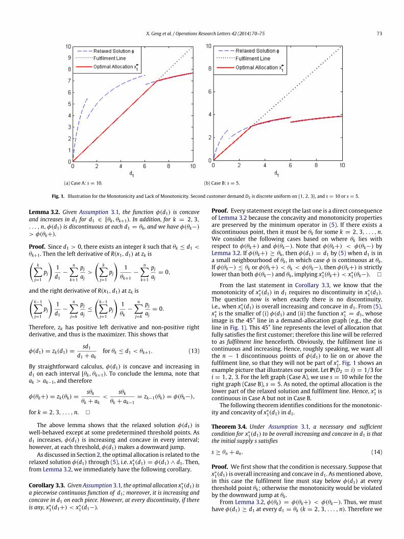
Fig. 1. Illustration for the Monotonicity and Lack of Monotonicity. Second customer demand D2 is discrete uniform on {1, 2, 3}, and s = 10 or s = 5.

Lemma 3.2. Given Assumption 3.1, the function φ(d1) is concaveand increases in d1 for d1 ∈ [θk, θk+1). In addition, for k = 2, 3,. . . , n, φ(d1) is discontinuous at each d1 = θk, and we have φ(θk−)

> φ(θk+).

Proof. Since d1 > 0, there exists an integer k such that θk ≤ d1 <θk+1. Then the left derivative of R(x1, d1) at zk is

kj=1

pj

1d1

−

nk+1

pjaj

>

k

j=1

pj

1

θk+1−

nk+1

pjaj

= 0,

and the right derivative of R(x1, d1) at zk isk−1j=1

pj

1d1

−

nj=k

pjaj

≤

k−1j=1

pj

1θk

−

nj=k

pjaj

= 0.

Therefore, zk has positive left derivative and non-positive rightderivative, and thus is the maximizer. This shows that

φ(d1) = zk(d1) =sd1

d1 + akfor θk ≤ d1 < θk+1. (13)

By straightforward calculus, φ(d1) is concave and increasing ind1 on each interval [θk, θk+1). To conclude the lemma, note thatak > ak−1, and therefore

φ(θk+) = zk(θk) =sθk

θk + ak<

sθkθk + ak−1

= zk−1(θk) = φ(θk−),

for k = 2, 3, . . . , n. �

The above lemma shows that the relaxed solution φ(d1) iswell-behaved except at some predetermined threshold points. Asd1 increases, φ(d1) is increasing and concave in every interval;however, at each threshold, φ(d1) makes a downward jump.

As discussed in Section 2, the optimal allocation is related to therelaxed solution φ(d1) through (5), i.e. x∗

1(d1) = φ(d1) ∧ d1. Then,from Lemma 3.2, we immediately have the following corollary.

Corollary 3.3. Given Assumption 3.1, the optimal allocation x∗

1(d1) isa piecewise continuous function of d1; moreover, it is increasing andconcave in d1 on each piece. However, at every discontinuity, if thereis any, x∗

1(d1+) < x∗

1(d1−).

Proof. Every statement except the last one is a direct consequenceof Lemma 3.2 because the concavity and monotonicity propertiesare preserved by the minimum operator in (5). If there exists adiscontinuous point, then it must be θk for some k = 2, 3, . . . , n.We consider the following cases based on where θk lies withrespect to φ(θk+) and φ(θk−). Note that φ(θk+) < φ(θk−) byLemma 3.2. If φ(θk+) ≥ θk, then φ(d1) = d1 by (5) when d1 is ina small neighbourhood of θk, in which case φ is continuous at θk.If φ(θk−) ≤ θk or φ(θk+) < θk < φ(θk−), then φ(θk+) is strictlylower than both φ(θk−) and θk, implying x∗

1(θk+) < x∗

1(θk−). �

From the last statement in Corollary 3.3, we know that themonotonicity of x∗

1(d1) in d1 requires no discontinuity in x∗

1(d1).The question now is when exactly there is no discontinuity,i.e., when x∗

1(d1) is overall increasing and concave in d1. From (5),x∗

1 is the smaller of (i) φ(d1) and (ii) the function x∗

1 = d1, whoseimage is the 45° line in a demand-allocation graph (e.g., the dotline in Fig. 1). This 45° line represents the level of allocation thatfully satisfies the first customer; therefore this line will be referredto as fulfilment line henceforth. Obviously, the fulfilment line iscontinuous and increasing. Hence, roughly speaking, we want allthe n − 1 discontinuous points of φ(d1) to lie on or above thefulfilment line, so that they will not be part of x∗

1 . Fig. 1 shows anexample picture that illustrates our point. Let P(D2 = i) = 1/3 fori = 1, 2, 3. For the left graph (Case A), we use s = 10 while for theright graph (Case B), s = 5. As noted, the optimal allocation is thelower part of the relaxed solution and fulfilment line. Hence, x∗

1 iscontinuous in Case A but not in Case B.

The following theorem identifies conditions for themonotonic-ity and concavity of x∗

1(d1) in d1.

Theorem 3.4. Under Assumption 3.1, a necessary and sufficientcondition for x∗

1(d1) to be overall increasing and concave in d1 is thatthe initial supply s satisfies

s ≥ θn + an. (14)

Proof. We first show that the condition is necessary. Suppose thatx∗

1(d1) is overall increasing and concave in d1. As mentioned above,in this case the fulfilment line must stay below φ(d1) at everythreshold point θk; otherwise the monotonicity would be violatedby the downward jump at θk.

From Lemma 3.2, φ(θk) = φ(θk+) < φ(θk−). Thus, we musthave φ(d1) ≥ d1 at every d1 = θk (k = 2, 3, . . . , n). Therefore we

74 X. Geng et al. / Operations Research Letters 42 (2014) 70–75

have the necessary conditionφ(θk) ≥ θk, for every k = 2, 3, . . . , n.Using Eq. (13), we can write it as sθk

θk+ak≥ θk, which reduces to

s ≥ ak + θk for every k = 2, 3, . . . , n. These inequalities areequivalent to the desired result s ≥ max2≤k≤n{ak + θk} = an + θn,where the last equality is due to the monotonicity of {ak} and {θk}

given in (6) and (12).Now we show the sufficiency. Suppose that the inequality

(14) holds. Then the deductions in the above proof are triviallyreversible from the last step up to the statement that φ(d1) ≥ d1at every d1 = θk (k = 2, 3, . . . , n). This means that the fulfilmentline is below the points (θk, φ(θk)), for each k = 2, 3, . . . , n.

We will conclude the proof by showing that x∗

1(d1) is overallincreasing and concave. Define θ = sup{d1 : φ(d1) ≥ d1}. Weclaim that φ(θ) = θ . If φ(θ) < θ , then by its definition, θ is apoint of discontinuity, which must be one of θk’s. This contradictsthe fact that φ(θk) ≥ θk. If φ(θ) > θ , then let δ = φ(θ) − θ > 0.Since by (13) φ(d1) is right continuous, we know that there existsan ϵ > 0, such that |φ(θ + ϵ) − φ(θ)| + ϵ ≤ δ. Hence, φ(θ + ϵ) ≥

φ(θ) + ϵ − δ = θ + ϵ, which contradicts the definition of θ .Therefore φ(θ) = θ , as claimed.

Now, since θ ≥ θk holds for every k = 2, 3, . . . , n, we haveθ ≥ θn. From Lemma 3.2, it follows that φ(θk−) > φ(θk) ≥ θk, fork = 2, 3, . . . , n. Hence, by the concavity of φ(d1) on each of theintervals [θk, θk+1) for k = 1, 2, . . . , n − 1, and [θn, θ ], we deducethat φ(d1) ≥ d1 for all 0 ≤ d1 ≤ θ . Therefore x∗

1(d1) = d1 on[0, θ ], which is increasing and linear. Besides, by the definition ofθ , φ(d1) < d1 for d1 > θ ; so x∗

1(d1) = φ(d1) when d1 > θ ≥ θn,which is increasing and concave according to Lemma 3.2. Finally,x∗

1(d1) is continuous at d1 = θ by noting that φ(θ) = θ . Moreover,since φ(d1) is below the fulfilment line after d1 = θ , we haveφ′(θ+) < 1 = φ′(θ−). Hence, x∗

1(d1) is overall increasing andconcave. �

This theorem shows that when the initial supply is sufficientlylarge, the optimal allocation is strictly increasing with the firstcustomer’s demand. Consider what would happen to the amountx1 allocated to customer 1 as the demand d1 increases. The supplierbalances the impact of two actions: (i) increase x1 to allocate moreto the first customer, and (ii) reservemore for the second customerby decreasing x1. (See our discussion following the definitions ofθk’s in (11).) Theorem 3.4 simply states that as long as the initialsupply is sufficient enough to meet the first demand up to θn (thehighest level of d1 for the supplier to consider the effect of (ii))and the second demand up to an (the largest realization of D2),respectively, the supplier can always allocate more to the firstcustomer as d1 increases. Conversely, the reasonwhy the allocationx1 could decrease even as d1 increases is that the initial supplyis limited — since the supplier’s action makes a more significantimpact on customer 2’s fill rate.

Alternately, using Eq. (11), the condition in Theorem 3.4 canbe written as s ≥

n−1j=1 pj/pn + 1

an. Let β =

n−1j=1 pj/pn +

1. Then, β is a constant that is completely determined by thedistribution of D2. Hence, the inequality s ≥ βan reveals theinterrelationship between the supply and the second distributionin affecting the structure of optimal allocation as a functionof the first demand. Furthermore, under many commonly seendistributions, the factor β is likely to be more than 2 because pnis generally smaller than 1 − pn. Therefore, if we let D1 and D2 beidentically distributed and β > 2, then the above condition meansthat the initial supply is sufficient enough to meet both customers’largest demands, which is why the supplier will not have to worryabout facing a large demand in the future while he increases x1.

In summary, Theorem 3.4 tells us sufficient initial supplyleads to an increasing optimal allocation function. Besides, thedistribution of D2 also plays a key role in that it determines bothθn and β . Note that condition (14) is possible to hold for some sbecause the realized demands are bounded; cf. Section 3.3.

Recall from (5) that x∗

1 is the minimum of two functions, φand the identity mapping. The condition in Theorem 3.4 ensuresthat the points of discontinuity in φ(d1) are not the points ofdiscontinuity in x∗

1(d1), and thus x∗

1(d1) is overall continuous.Meanwhile, we are interested to see when the function x∗

1(d1)would be determined by φ(d1) instead, i.e., x∗

1(d1) = φ(d1). In thiscase, x∗

1(d1) becomes discontinuous at every θk (k = 2, 3, . . . , n).Besides, the optimal allocation stays below the fulfilment line;i.e., the first customer is never fully satisfied. Intuitively, thiswouldhappen when the second period demand is much larger than theinitial supply. Because the second customer’s fill rate will neverreach 1, there is no need for the supplier to allocate to the firstcustomer the full demanded amount, regardless how small it is.The above intuition is verified in the following proposition.

Proposition 3.5. Suppose that Assumption 3.1 holds. If s ≤ a1, thenx∗

1(d1) = φ(d1) < d1 for d1 > 0.

Proof. For any d1 > 0, there is some k such that φ(d1) = zk(d1) by(13). Hence, if s ≤ a1, then by differentiating Eq. (13), φ′(d1+) =

sak/(d1 + ak)2 < sak/a2k < s/a1 ≤ 1, where the second inequalityfollows from (6). In particular,φ′(0+) = s/a1 ≤ 1. Besides,φ(0) =

0. Therefore, combining the result in Lemma 3.2, we conclude thatφ(d1) intersects with the fulfilment line only at d1 = 0; sinceφ(d1) < d1 holds for d1 > 0. By (5), we conclude the result. �

If the initial supply is neither too large nor too small comparedto the second demand (thus Theorem 3.4 and Proposition 3.5are inapplicable), we have to combine Eq. (5) and Lemma 3.2 tosee where x∗

1 is increasing in d1 and where the discontinuousdownward jump occurs.

3.3. Unbounded discrete distribution

In the earlier discussion, an (themaximumpossible value ofD2),has played an important role in characterizing the monotonicitycondition for the optimal allocation. In fact, an being finite isthe main reason why inequality (14) can hold for some s. Thissubsection focuses on the case where the second period demandis discrete but unbounded (e.g. Poisson distribution). We use thisassumption throughout this subsection.

Assumption 3.6. D2 is discretely distributed, and P(D2 > M) > 0for any M ≥ 0.

We will use the same notations as defined in the previoussubsection, with slight modifications to adapt to the unboundedcase. To be specific, instead of being finitely many, all sequences{ak}, {zk} and {θk} have infinitely many points. For instance, theprobability mass function of D2 becomes P(D2 = ak) = pk > 0 fork = 1, 2, . . . with {ak} strictly increasing to +∞. Besides, θk nowtakes the form that θk =

k−1j=1 pj

/

∞

j=k pj/aj. Note that θk

is well-defined because the series in the denominator converges.Moreover, it can be shown that each θk is finite, but {θk} is anincreasing and unbounded sequence of positive numbers.

Because of the infinitely many break points {zk} of the objectivefunction, the function φ(d1) now has infinitely many continuouspieces. Each of the piece is strictly increasing and concave in d1,and each discontinuous point sees a decrease in function value.In other words, Lemma 3.2 basically remains the same underAssumption 3.6, except that there are now infinitely many θk’s.

X. Geng et al. / Operations Research Letters 42 (2014) 70–75 75

In contrast, for the optimal allocation x∗

1 , there is an interestingdifference from Theorem 3.4. The condition (14) in the previouscase holds for some s, whereas it can never hold for any s in theunbounded case, simply because s can never be larger than the‘‘largest’’ demand realization. Therefore, the overall continuity cannever happen under Assumption 3.6. We present it as the nexttheorem.

Theorem 3.7. Under Assumption 3.6, given any initial supply s, thereexists d1 > 0 such that x∗

1(d1) is discontinuous at d1 = d1. Moreover,x∗

1(d1−) > x∗

1(d1).

Proof. Since ak and θk both strictly increase to infinity, we knowthat for any s > 0, there exists an integer k > 0 such that

s < ak−1 + θk. (15)

Then by Eq. (13), we have

φ(θk) = zk(θk) =sθk

θk + ak<

sθkθk + ak−1

= zk−1(θk−) = φ(θk−).

Apply inequality (15) to deduce φ(θk) < φ(θk−) = sθk/(θk +

ak−1) < θk. Hence by Eq. (5), x∗

1(θk) = φ(θk) ∧ θk = φ(θk) whilex∗

1(θk−) = φ(θk−) ∧ θk = φ(θk−). Since φ(θk) < φ(θk−), itfollows that x∗

1(d1) is discontinuous at d1 = θk. Letting d1 = θkproves the theorem. �

The above theorem shows that the unboundedness of D2 (As-sumption 3.6) plays an important role. Suppose that the incrementfrom ak−1 to ak remains constant for each k. Then, it can be seenfrom the proof of Theorem 3.7 that zk(θk) → s as d1 → +∞

for every k, we know that the discontinuity gaps of φ(d1) becomesmaller as d1 gets larger. However, because the distribution is dis-crete, there are always positive gaps. This leads to the inevitablediscontinuity of the optimal allocation. The discussion under The-orem 3.4 shows that if the optimal allocation is continuous in alld1 > 0, then the initial supply must be large enough compared tothe second demand. Hence, under unbounded assumption, it is ex-pected that condition (14) will never hold because the probabilityof D2 being very large is positive and s cannot exceed it.

Meanwhile, Proposition 3.5 continues to hold. This is becausethe result depends on the relationship between the initial supplyand the smallest realization of the second demand, a1. Since a1 is

a fixed finite number, unless a1 = 0, there exists some s > 0 suchthat s ≤ a1.

Acknowledgements

The authors acknowledge helpful comments from SridharSeshadri and the review team, as well as the support from NaturalSciences and Engineering Council of Canada.

References

[1] A. Alkan, G. Demange, D. Gale, Fair allocation of indivisible goods and criteriaof justice, Econometrica 59 (4) (1991) 1023–1039.

[2] A.B. Atkinson, On the measurement of inequality, J. Econom. Theory 2 (3)(1970) 244–263.

[3] D.P. Bertsekas, R.G. Gallager, P. Humblet, Data Networks, Vol. 2, Prentice-HallInternational, 1992.

[4] D. Bertsimas, V.F. Farias, N. Trichakis, The price of fairness, Oper. Res. 59 (1)(2011) 17–31.

[5] D. Bertsimas, V.F. Farias, N. Trichakis, On the efficiency-fairness trade-off,Manag. Sci. 58 (12) (2012) 2234–2250.

[6] A.M. Campbell, D. Vandenbussche, W. Hermann, Routing for relief efforts,Transp. Sci. 42 (2) (2008) 127–145.

[7] Y. Chevaleyre, P. Dunne, U. Endriss, J. Lang, M. Lemaitre, N.Maudet, J. Padget, S.Phelps, J. Rodriguez-Aguilar, P. Sousa, Issues inmultiagent resource allocation,Informatica 30 (1) (2006).

[8] F.P. Kelly, A.K. Maulloo, D.K. Tan, Rate control for communication networks:shadow prices, proportional fairness and stability, J. Oper. Res. Soc. 49 (3)(1998) 237–252.

[9] R.W. Lien, Design and control principles for distribution systems: studies incommercial & nonprofit operations, Ph.D. Thesis, Northwestern University,2008.

[10] R.W. Lien, S.M.R. Iravani, K.R. Smilowitz, Sequential resource allocation fornonprofit operations, Working paper, 2008.

[11] H. Luss, On equitable resource allocation problems: a lexicographic minimaxapproach, Oper. Res. 47 (3) (1999) 361–378.

[12] A. Mas-Collel, M.D. Whinston, J. Green, Microeconomic Theory, OxfordUniversity Press, Oxford, 1995.

[13] J.F. Nash, The bargaining problem, Econometrica (1950) 155–162.[14] J. Rawls, A Theory of Justice, Harvard University Press, Cambridge, MA, 1971.[15] E.S. Savas, On equity in providing public services, Manag. Sci. 24 (8) (1978)

800–808.[16] S. Solak, C. Scherrer, A. Ghoniem, The stop-and-drop problem in nonprofit food

distribution networks, Ann. Oper. Res. (2012) 1–20.[17] J.M. Swaminathan, Decision support for allocating scarce drugs, Interfaces 33

(2) (2003) 1–11.[18] K.T. Talluri, G. Van Ryzin, The Theory and Practice of Revenue Management,

Springer Verlag, 2005.[19] H.P. Young, Equity: In Theory and Practice, Princeton University Press,

Princeton, NJ, 1995.