sequential optimizing strategy in multi-dimensional bounded forecasting games

Stochastic Processes and their Applications 121 (2011) 155–183www.elsevier.com/locate/spa

Sequential optimizing strategy in multi-dimensionalbounded forecasting games

Masayuki Kumon, Akimichi Takemuraa,∗, Kei Takeuchib

a Graduate School of Information Science and Technology, University of Tokyo, 7-3-1 Hongo, Bunkyo-ku,Tokyo 113-8656, Japan

b Emeritus, Graduate School of Economics, University of Tokyo, Japan

Received 1 June 2010; received in revised form 25 August 2010; accepted 19 September 2010Available online 25 September 2010

Abstract

We propose a sequential optimizing betting strategy in the multi-dimensional bounded forecasting gamein the framework of game-theoretic probability of Shafer and Vovk (2001) [10]. By studying the asymptoticbehavior of its capital process, we prove a generalization of the strong law of large numbers, where theconvergence rate of the sample mean vector depends on the growth rate of the quadratic variation process.The growth rate of the quadratic variation process may be slower than the number of rounds or may evenbe zero. We also introduce an information criterion for selecting efficient betting items. These results arethen applied to multiple asset trading strategies in discrete-time and continuous-time games. In the case ofa continuous-time game we present a measure of the jaggedness of a vector-valued continuous process. Ourresults are examined by several numerical examples.c⃝ 2010 Elsevier B.V. All rights reserved.

Keywords: Game-theoretic probability; Holder exponent; Information criterion; Kullback–Leibler divergence; Quadraticvariation; Strong law of large numbers; Universal portfolio

1. Introduction

Since the advent of the game-theoretic probability and finance by Shafer and Vovk [10], thefield has been expanding rapidly. The present authors have been contributing to this emergingfield by showing the essential role of the Kullback–Leibler divergence for the strong law of large

∗ Corresponding author.E-mail addresses: masayuki [email protected] (M. Kumon), [email protected] (A. Takemura).

0304-4149/$ - see front matter c⃝ 2010 Elsevier B.V. All rights reserved.doi:10.1016/j.spa.2010.09.004

http://dx.doi.org/10.1016/j.spa.2010.09.004

http://www.elsevier.com/locate/spa

mailto:[email protected]

mailto:[email protected]

http://dx.doi.org/10.1016/j.spa.2010.09.004

156 M. Kumon et al. / Stochastic Processes and their Applications 121 (2011) 155–183

numbers (SLLN) [7,8] and by proposing a new approach to continuous-time games [13,14]. Ourapproach to continuous-time games has been further developed by Vovk [16–19]. By these worksit has now become clear that game-theoretic no-arbitrage condition implies many properties ofidealized continuous price paths without any probabilistic assumptions.

In this paper we propose a sequential optimizing betting strategy for the multi-dimensionalbounded forecasting game in discrete time and apply it as a high-frequency limit order typebetting strategy for vector-valued continuous price processes.

Our strategy is very flexible and the analysis of its asymptotic behavior allows us to generalizegame-theoretic statements of SLLN to a wide variety of cases. SLLN for the bounded forecastinggame is already established in Chapter 3 of [10]. In [7] we gave a simple strategy forcing SLLNwith the rate of O(

log n/n), where n is the number of rounds. However the convergence rate of

SLLN should depend on the growth rate of the quadratic variation process. For example, in viewof Kolmogorov’s three series theorem (e.g. Section IV.2 of [11]), the sum sn = x1+· · ·+xn ∈ R1

of centered independent measure-theoretic random variables converges a.s. if the sum of theirvariances converges (i.e.

∑n Var(xn) < ∞). Therefore in this case the sample average xn = sn/n

is of order O(1/n). By our sequential optimizing betting strategy, we can give a unified game-theoretic treatment on the asymptotic behavior of sn , which depends on the asymptotic behaviorof the observed sum of squares

∑ni=1 x2

i as n → ∞.The strength of our results can be seen when we interpret our results in the standard measure-

theoretic framework. By the generality of probability games (Chapter 8 of [10]), our game-theoretic result can be immediately translated into measure-theoretic statements. Let sn =

x1 + · · · + xn be a one-dimensional measure-theoretic martingale w.r.t. a filtration Fn withuniformly bounded differences |xn| ≤ 1, a.e. Let Vn = x2

1 + · · · + x2n . Then with probability one

the sequence |sn|/

max(1, Vn log Vn), n = 1, 2, . . . , is bounded. See Proposition 2.1 below.Note that in this statement no assumption is made on the growth rate of Vn . The rate itself maybe random. In the measure-theoretic framework the law of the iterated logarithm for martingaleswas proved by [12,15]. Our rate

Vn log Vn is weaker. However the measure-theoretic results

compare sn to the sum of conditional variances∑n

i=1 E(x2i |Fi−1), whereas in our result Vn is

the observed sum of squares. As far as we know, our result involving Vn is new also in themeasure-theoretic framework.

From a more practical viewpoint, our sequential betting strategy is very simple to implementeven for high dimensions and shows a very competitive performance when applied to variousprice processes. In Section 6 we compare the performance of our strategy with the well-knownuniversal portfolio strategy developed by Cover [3], Cover and Ordentlich [4], Ordentlich andCover [9] and Cover and Thomas [5]. The performance of our sequential betting strategyis competitive against the universal portfolio. Note that the numerical integration needed forimplementing the universal portfolio is computationally heavy for high dimensions.

When we can bet on a large number of price processes, it is not always best to form a portfoliocomprising all price processes, because estimating the best weight vector for the price processesmight take a long time. By approximating the capital process of our sequential optimizingstrategy, we will introduce an information criterion for selecting price processes in a portfolio.

The organization of this paper is as follows. In Section 2 we formulate the multi-dimensionalbounded forecasting game, introduce our sequential optimizing strategy and state our maintheoretical result. In Section 3 we give a proof of our result by analyzing the asymptotic behaviorof its capital process. We also introduce an information criterion for selecting efficient bettingitems. These results are then applied to multiple asset trading games in Section 4. In Section 4 we

M. Kumon et al. / Stochastic Processes and their Applications 121 (2011) 155–183 157

formulate the multiple asset trading game in continuous time and based on high-frequency limitorder type betting strategies we present a measure for the jaggedness of a path of a vector-valuedcontinuous process. In Section 5, to indicate the generality of our results, we provide a multi-dimensional Girsanov theorem for geometric Brownian motion and an argument concerning themutual information between betting games. In Section 6 we give numerical results for severalJapanese stock price processes. We conclude the paper with some discussions in Section 7.

2. A sequential optimizing strategy that forces a new strong law of large numbers

We treat the following type of discrete-time bounded forecasting game between Skeptic andReality. K0 is Skeptic’s initial capital, D is a compact region in Rd such that its convex hull coDcontains the origin in its interior, and · denotes the standard inner product of Rd .

DISCRETE-TIME BOUNDED FORECASTING GAME

Protocol:

K0 := 1.FOR n = 1, 2, . . .:Skeptic announces Mn ∈ Rd .Reality announces xn ∈ D.Kn = Kn−1 + Mn · xn .

END FOR

In this paper we regard d-dimensional vectors such as xn = (x1n , . . . , xd

n )t as column vectorswith t denoting the transpose. ‖x‖ =

√x tx =

√x · x denotes the Euclidean norm of x . Letting

αn = Mn/Kn−1, we can rewrite Skeptic’s capital as Kn = Kn−1(1 + αn · xn), αn ∈ Rd . In theprotocol, we require that Skeptic observes his collateral duty, in the sense that Kn ≥ 0 for all nirrespective of Reality’s moves x1, x2, . . . .

For constructing a strategy of Skeptic, assume that Skeptic himself generates ‘training data’x−n0+1, x−n0+2, . . . , x0 of size n0 ≥ d + 1. This operation is similar to a construction of aprior distribution in Bayesian statistics, where a prior distribution can be specified by a set ofprior observations. Throughout this paper we fix arbitrarily ϵ0 ∈ (0, 1) and choose the trainingdata x−n0+1, . . . , x0 in such a way that

1 + α · xn ≥ 0, n = −n0 + 1, . . . , 0 ⇒ 1 + α · x ≥ ϵ0, ∀x ∈ D. (1)

Let Pdn0,ϵ0

= α | 1 + α · xn ≥ 0, n = −n0 + 1, . . . , 0. Then (1) is equivalent to

Pdn0,ϵ0

⊂ −(1 − ϵ0)(co D)⊥,

where (co D)⊥ denotes the convex dual of co D. For example, for d = 1 and D = [−1, 1], wecan take x−1 = 1/(1 − ϵ0) and x0 = −1/(1 − ϵ0). Then α has to satisfy |α| ≤ 1 − ϵ0 and theright-hand side of (1) holds. For general D ⊂ Rd let δ = maxx∈D ‖x‖ and let c = δ

√d/(1−ϵ0).

Then we can take n0 = 2d training vectors as

(0, . . . , 0, ±c, 0, . . . , 0)t,

where c is in the i-th coordinate (1 ≤ i ≤ d). Then each element αi , 1 ≤ i ≤ d , ofα = (α1, . . . , αd)t has to satisfy |αi

| ≤ 1/c and ‖α‖ ≤ (1 − ϵ0)/δ. Hence the right-handside of (1) holds by Cauchy–Schwarz inequality. It should also be noted that (1) implies that thetraining vectors span the whole Rd .


The strategy with a constant vector αn ≡ α ∈ Rd is called a constant proportional bettingstrategy. For N ≥ 0 we define

Φ0,N (α) =

N−n=−n0+1

log(1 + α · xn), (2)

which is the log capital at round N under the constant proportional betting strategy, includingthe training data. We add ‘0’ to the subscript to indicate that the training data are included in asummation. Since the game starts at time 1, actually the log capital of the constant proportionalbetting strategy is Φ0,N (α) − Φ0,0(α) =

∑Nn=1 log(1 + α · xn).

Let us consider the maximization of Φ0,N (α) with respect to α ∈ Rd . The maximumcorresponds to the log capital at time N of a ‘hindsight’ constant proportional betting strategy.Note that Φ0,N (α) is a strictly concave function of α. The condition (1) ensures that the maximumof Φ0,N (α) is attained at the unique point α = α∗

N in the interior of Pdn0,ϵ0

so that

∂Φ0,N

∂α

α=α∗

N

=

N−n=−n0+1

xn

1 + α∗

N · xn= 0. (3)

From a numerical viewpoint we note that the maximization of Φ0,N (α) is straightforward evenin high dimensions.

We now define the sequential optimizing strategy (SOS) of Skeptic, which is a realizablestrategy unlike the hindsight strategy. It is given by

αn = α∗

n−1, n ≥ 1. (4)

The idea of SOS is very simple. We employ the empirically best constant proportion until theprevious round for betting at the current round. Note that SOS depends on the choice of thetraining data. Skeptic’s log capital log K∗

1,N at round N under SOS is written as

log K∗

1,N =

N−n=1

log(1 + α∗

n−1 · xn).

Let ξ = x1x2 · · · ∈ D∞ denote a path, which is an infinite sequence of Reality’s moves.The set Ω = D∞ of paths is called the sample space and any subset E of Ω is calledan event. ξn

= x1 . . . xn denotes a partial path of Reality until the round n. A strategy Pspecifies αn in terms of ξn−1, i.e. αn = P(ξn−1). The capital process under P is given asK P

1,N =∏N

n=1(1 + P(ξn−1) · xn). P is called prudent, if Skeptic observes his collateral duty

by P , i.e. K P1,N ≥ 0, ∀N ≥ 0, irrespective of Reality’s moves x1, x2, . . . . In this paper we only

consider prudent strategies for Skeptic. We say that Skeptic can weakly force an event E ⊂ Ωby a strategy P if lim supN K P

1,N = ∞ for every ξ ∈ E . As in Section 1 we write

sN = x1 + · · · + xN ∈ Rd , VN = x1x t1 + · · · + xN x t

N (: d × d). (5)

Then tr VN =∑N

n=1 ‖xn‖2. We are now ready to state our main theorem.

Theorem 2.1. The sequential optimizing strategy for Skeptic weakly forces

E : lim supN

‖sN ‖max(1, tr VN log(tr VN ))

< ∞. (6)


The maximum in the denominator is needed only for the case that supN tr VN ≤ 1, such aswhen 0 ∈ D and Reality always chooses xn ≡ 0. It is important to emphasize that E in (6) isweakly forced irrespective of the rate of growth of tr VN , including the zero-growth case, i.e. thecase that tr VN converges to a finite value. A measure-theoretic interpretation of our result showsits flexibility. When xn’s are measure-theoretic martingale differences, then the capital processunder SOS is a non-negative measure-theoretic martingale, which converges to a finite valuealmost surely. The method for deriving measure-theoretic from game-theoretic results explainedin Chapter 8 of [10] allows us to derive the following proposition from Theorem 2.1.

Proposition 2.1. Let sn = x1 + · · · + xn be a d-dimensional measure-theoretic martingalew.r.t. a filtration Fn. Assume that the differences xn ∈ D are uniformly bounded a.e. Thenwith probability one the sequence ‖sn‖/

max(1, tr Vn log(trVn)), n = 1, 2, . . . , is bounded.

Let λmax,N and λmin,N denote the maximum and the minimum eigenvalues of VN . Considerthe event

E ′: lim

N

log λmax,N

λmin,N= 0. (7)

Theorem 2.1 gives only the order of sN . If we condition the paths on the event E ′, then we canderive a more accurate numerical bound as follows.

Theorem 2.2. By the sequential optimizing strategy Skeptic can weakly force

E ′⇒ lim sup

N

stN V −1

N sN

log |VN |≤ 1.

This theorem follows from the fact that on E ′ Skeptic can weakly force α∗

N → 0, as shown inthe proof of this theorem in Section 3.4.

Note that λmin,N → ∞ on E ′. Note also that E in (6) holds if and only iflim supN ‖sN ‖/

max(1, λmax,N log λmax,N ) < ∞, because λmax,N ≤ tr VN ≤ dλmax,N . Hence

on E ′ we have

1 ≥ lim supN

stN V −1

N sN

log |VN |≥ lim sup

N

‖sN ‖2

dλmax,N log λmax,N.

Therefore, although we only have a conditional statement in Theorem 2.2, it gives a moreaccurate numerical bound than Theorem 2.1.

3. Proof of the theorem and some other results on sequential optimizing strategy

In this section we provide proofs of the above theorems and present other results on thesequential optimizing strategy.

3.1. Properties of α∗

N and the empirical risk neutral distribution

Let δx denote a unit point mass at x ∈ Rd and let gN =∑N

n=−n0+1 δxn /(N + n0) denotethe empirical distribution of the training data and Reality’s moves x1, . . . , xN up to round N . Inview of (3) we define the empirical risk neutral distribution g∗

N up to round N by

g∗

N =1

N + n0

N−n=−n0+1

δxn

1 + α∗

N · xn.


For notational simplicity we omit ‘0’ from the subscript of gN and g∗

N , although they involve thetraining data. g∗

N is indeed a probability measure, because by (3) we have

−xn

g∗

N (xn) =1

N + n0

N−n=−n0+1

11 + α∗

N · xn=

1N + n0

N−n=−n0+1

1 + α∗

N · xn

1 + α∗

N · xn= 1,

where the summation on the left-hand side is over distinct values of xn , n = −n0 + 1, . . . , N .By Eg∗

N[·] we denote the expected value under g∗

N . Then (3) is written as Eg∗N[x] = 0.

The log capital log K∗

0,N = Φ0,N (α∗

N ) of the constant hindsight strategy α∗

N up to round Nincluding the training data is expressed as

log K∗

0,N = Φ0,N (α∗

N ) = (N + n0)−xn

gN (xn) loggN (xn)

g∗

N (xn)

= (N + n0)D(gN ‖ g∗

N ), (8)

where D(gN ‖ g∗

N ) denotes the Kullback–Leibler divergence between two probabilitydistributions gN and g∗

N .Now note that log(1 + α∗

n−1 · xn) = Φ0,n(α∗

n−1) − Φ0,n−1(α∗

n−1). By summation by parts, thedifference log K∗

0,N − log K∗

1,N between the hindsight strategy and SOS can be expressed as

log K∗

0,N − log K∗

1,N =

N−n=1

1Φn + Φ0,0(α∗

0), (9)

where 1Φn = Φ0,n(α∗n) − Φ0,n(α∗

n−1) ≥ 0 and Φ0,0(α∗

0) is a constant depending only on thetraining data. We will analyze the behavior the log capital log K∗

1,N of SOS by analyzing log K∗

0,N

and∑N

n=0 1Φn .We call

V ∗

N =1

N + n0V ∗

0,N = Eg∗N[xx t

] =1

N + n0

N−n=−n0+1

xn x tn

1 + α∗

N · xn

the empirical risk neutral covariance matrix for Reality’s moves up to round N . Write

s0,N =

N−n=−n0+1

xn, x0,N =1

N + n0s0,N .

Noting gN (xn) = (1 + α∗

N · xn)g∗

N (xn), we have

x0,N = EgN [x] = Eg∗N[(1 + α∗

N · x)x] = Eg∗N[x] + Eg∗

N[xx t

]α∗

N = Eg∗N[xx t

]α∗

N .

Therefore α∗

N is expressed as

α∗

N = V ∗−1N x0,N = V ∗−1

0,N s0,N . (10)

Since V ∗

N itself contains α∗

N , (10) does not give an explicit expression of α∗

N . However it is a veryuseful exact relation for our analysis.

We now consider 1α∗n = α∗

n − α∗

n−1. In the following we use the notation

xn(α) =xn

1 + α · xn.


Taking the difference of the following two equalities

0 =

n−i=−n0+1

xi (α∗n), 0 =

n−1−i=−n0+1

xi (α∗

n−1)

we obtain

0 =

n−1−i=−n0+1

xi(α∗

n−1 − α∗n) · xi

(1 + α∗

n−1 · xi )(1 + α∗n · xi )

+ xn(α∗n).

Thereforen−1−

i=−n0+1

xi x ti

(1 + α∗

n−1 · xi )(1 + α∗n · xi )

(α∗

n − α∗

n−1) = xn(α∗n).

Note that the denominator on the left-hand side is a scalar and the matrix on the left-hand side ispositive definite. Then

1α∗n = V0,n−1(α

∗

n−1, α∗n)−1xn(α∗

n), (11)

where V0,n−1(α, β) =∑n−1

i=−n0+1 xi (α)xi (β)t.Concerning the behavior of 1α∗

n we state the following lemma, which will be used inSection 3.4.

Lemma 3.1. limn 1α∗n = 0 for every ξ ∈ D∞.

We give a proof of this lemma in Appendix.

3.2. Bounding the difference between the hindsight strategy and SOS from above

We now give a detailed analysis of∑N

n=1 1Φn on the right-hand side of (9) and bound it fromabove. We note the following simple fact on 1Φn :

1Φ,n = Φ0,n(α∗n) − Φ0,n(α∗

n−1) = Φ0,n−1(α∗n) − Φ0,n−1(α

∗

n−1) + log1 + α∗

n · xn

1 + α∗

n−1 · xn

≤ log1 + α∗

n · xn

1 + α∗

n−1 · xn= log

1 +

1α∗n · xn

1 + α∗

n−1 · xn

, (12)

where the inequality holds since α∗

n−1 maximizes Φn−1(α). Substituting (11) into the right-handside we obtain

1Φn ≤ log(1 + xn(α∗n)tV0,n−1(α

∗

n−1, α∗n)−1xn(α∗

n−1)). (13)

Note that we can also rewrite

1 + xn(α∗n)tV0,n−1(α

∗

n−1, α∗n)−1xn(α∗

n−1) =|V0,n(α∗

n−1, α∗n)|

|V0,n−1(α∗

n−1, α∗n)|

, (14)

where we used a well-known relation between determinants (e.g. Corollary A.3.1 of [1]).


Let

C1 = max

supα∈−(co D)⊥, x∈D

(1 + α · x), sup−n0+1≤n≤0

α∈Pdn0,ϵ0

(1 + α · xn)

, (15)

which is a constant depending only on the training data. The first argument C1,0 =

supα∈−(co D)⊥, x∈D(1 + α · x) on the right-hand side of (15) corresponds to the maximum one-step growth rate of Skeptic’s capital under the collateral duty and C1,0 equals 2 if D is symmetricw.r.t. the origin. C1,0 may be large if D is highly asymmetric w.r.t. the origin. For example, ford = 1 and D = [−0.1, 1], we have C1,0 = 11.

For two symmetric matrices A, B, let A ≥ B mean that A − B is non-negative definite. Then

V0,n−1(α∗

n−1, α∗n) ≥

1

C21

V0,n−1,

where V0,n−1 = V0,n−1(0, 0) =∑n

i=−n0+1 xi x ti . Note that V0,n−1 is positive definite because

of the training data, although Vn−1 in (5) may be singular. Note also that 1 + α∗m · xn ≥ ϵ0 for

m, n ≥ 1. Therefore

xn(α∗n)tV0,n−1(α

∗

n−1, α∗n)−1xn(α∗

n−1) ≤ C2x tn V −1

0,n−1xn, C2 =C2

1

ϵ20

.

Hence we can boundN−

n=1

1Φn ≤

N−n=1

log(1 + C2x tn V −1

0,n−1xn).

Write an = x tn V −1

0,n−1xn ≥ 0. Note that 1 + an = |V0,n|/|V0,n−1|. Also for c ≥ 1 and a ≥ 0 wehave 1 + ac ≤ (1 + a)c and hence

log(1 + ac) ≤ c log(1 + a).

ThereforeN−

n=1

log(1 + C2an) ≤ C2

N−n=1

log(1 + an) = C2 log|V0,N |

|V0,0|.

Now we have proved the following lemma.

Lemma 3.2. The difference∑N

n=1 1Φn on the right-hand side of (9) is bounded from above as

N−n=1

1Φn ≤ C2(log |V0,N | − log |V0,0|).

Since |V0,N | involves the training data, for simplicity in our statement we further boundit as follows. By the inequality between the geometric mean and arithmetic mean we have|V0,N |

1/d≤ tr V0,N /d. Hence

log |V0,N | ≤ d log tr V0,N − d log d = d log(tr VN + tr V0,0) − d log d

≤ d log(tr VN + tr V0,0).


If tr VN ≤ 1, then log(tr VN + tr V0,0) ≤ log(1+ trV0,0) ≤ tr V0,0. On the other hand if tr VN > 1,then

log(tr VN + tr V0,0) = log tr VN + log

1 +tr V0,0

tr VN

≤ log tr VN +

tr V0,0

tr VN

≤ log tr VN + tr V0,0.

Therefore for both cases log |V0,N | ≤ d max(0, log tr VN ) + dtr V0,0. Let C3 = C2(dtr V0,0 −

log |V0,0|). In summary we have the following bound.

Lemma 3.3. The difference∑N

n=1 1Φn on the right-hand side of (9) is bounded from above as

N−n=1

1Φn ≤ dC2 max(0, log tr VN ) + C3, (16)

where C2, C3 depend only on the training data.

Note that (16) is true even for the case that limN tr VN < ∞. Note also that log tr VN is oforder O(log N ) even for VN = O(N γ ), 0 < γ < 1. However for trVN = log N we havelog tr VN = log log N .

3.3. Bounding the hindsight strategy from below

In this subsection we bound the hindsight strategy from below and thus finish the proof ofTheorem 2.1.

Consider the function (1 + t) log(1 + t), t > −1. By the Taylor expansion we have

(1 + t) log(1 + t) = t +12

t2

1 + θ t, 0 < θ < 1.

By the definition of C1 in (15) we have

(1 + α∗

N · xn) log(1 + α∗

N · xn) ≥ α∗

N · xn +(α∗

N · xn)2

2C1,

∀N ≥ 1, − n0 + 1 ≤ ∀n ≤ N ,

and

Φ0,N (α∗

N ) =

N−n=−n0+1

(1 + α∗

N · xn) log(1 + α∗

N · xn)1

1 + α∗

N · xn

≥

N−n=−n0+1

α∗

N · xn

1 + α∗

N · xn+

12C1

N−n=−n0+1

(α∗

N · xn)2

1 + α∗

N · xn

=1

2C1

N−n=−n0+1

(α∗

N · xn)2

1 + α∗

N · xn, (17)

where we have used the fact Eg∗N[x] = 0. By (10) the summation on the right-hand side can be

written as

N−n=−n0+1

(α∗

N · xn)2

1 + α∗

N · xn= α∗ t

N V ∗

0,N α∗

N = α∗ tN s0,N = st

0,N V ∗−10,N s0,N . (18)


In analyzing the behavior of (18) we need to be careful about the following fact: 1 + α∗

N · xn ,n ≤ 0, may be arbitrarily close to zero for the training data x−n0+1, . . . , x0. In particular wemight have different behavior between eigenvalues of V ∗

0,N and and those of VN . To assess theeffect of training data let

AN =

0−n=−n0+1

11 + α∗

N · xn

and define the following event

E1 : lim supN

AN

max(1, log tr VN )< ∞.

Again max is needed only for the case that tr VN ≤ 1 for all N . We now show that Skepticcan weakly force E1. Fix an arbitrary ξ ∈ Ec

1, where Ec1 denotes the complement of E1. Then

lim supN AN / max(1, log tr VN ) = ∞ and hence there exists some n1 ≤ 0 such that

lim supN

1/(1 + α∗

N · xn1)

max(1, log tr VN )= ∞.

Then there exits a subsequence of rounds N1 < N2 < · · · such that

limk

1/(1 + α∗

Nk· xn1)

max(1, log tr VNk )= ∞.

Because α∗

Nk· xn1 → −1 we have

lim supN

(α∗N ·xn1 )2

1+α∗N ·xn1

max(1, log tr VN )= ∞.

If we compare this with the left-hand side of (18), we see that a single term xn1 of the trainingdata contributes arbitrary large gain to Skeptic in comparison to the right-hand side of (16). Thisimplies that lim supN log K∗

1,N = ∞. We have proved that by SOS Skeptic can weakly force E1.Therefore from now we only consider ξ ∈ E1.

At this point we distinguish two cases (1) E2 : limN tr VN < ∞ or (2) Ec2 : limN tr VN = ∞.

Consider the first case and fix an arbitrary ξ ∈ E2 ∩ E1. For such a ξ there exists δ(ξ) > 0 suchthat lim infN (1 + α∗

N · xn) ≥ δ(ξ) for all n < 0. Then

V ∗

0,N ≤1

max(ϵ0, δ(ξ))

N−n=−n0+1

xn x tn

and hence the maximum eigenvalue λmax,0,N of V ∗

0,N is bounded. Then

st0,N V ∗−1

0,N s0,N ≥‖s0,N ‖

2

λmax,0,N

and lim supN log K∗

1,N = ∞ if lim supN ‖s0,N ‖2

= ∞. Noting that lim supN ‖s0,N ‖2

= ∞ if

and only if lim supN ‖sN ‖2

= ∞, we have shown that by SOS Skeptic can weakly force

limN

tr VN < ∞ ⇒ lim supN

‖sN ‖2 < ∞.


Now consider the second case Ec2 ∩ E1. On Ec

2 ∩ E1

limN

log tr VN

tr VN= 0

always holds. Also on Ec2 ∩ E1

lim supN

tr V0,0(α∗

N )

log tr VN< ∞ where V0,0(α

∗

N ) =

0−n=−n0+1

xn x tn

1 + α∗

N · xn.

Therefore on Ec2 ∩ E1

limN

tr V0,0(α∗

N )

tr VN= 0.

Also

tr(V ∗

0,N − V0,0(α∗

N )) ≤1ϵ0

tr VN ,

and hence on Ec2 ∩ E1

lim supN

tr V ∗

0,N

tr VN= lim sup

N

tr V0,0(α∗

N ) + tr (V ∗

0,N − V0,0(α∗

N ))

tr VN≤

1ϵ0

.

Now on the right-hand side of (18), for every ξ ∈ Ec2 ∩ E1 there exists N0 = N0(ξ) such that

for all n ≥ N0

Φ0,N (α∗

N ) ≥1

2C1

‖s0,N ‖2

tr V ∗

0,N≥

ϵ0

4C1

‖s0,N ‖2

tr VN.

Hence if for this ξ

lim supN

‖s0,N ‖2

tr VN log tr VN= ∞

then lim sup log K∗

1,N = ∞ in view of Lemma 3.3. However on Ec2 the following two events are

equivalent:

lim supN

‖s0,N ‖2

tr VN log tr VN= ∞ ⇔ lim sup

N

‖sN ‖2

tr VN log tr VN= ∞.

This completes the proof of Theorem 2.1.

3.4. Better approximation to the capital process of SOS

Note that (13) is convenient because it gives an upper bound which always holds. Howeverbounding by Φ0,n(α∗

n) − Φ0,n(α∗

n−1) ≤ 0 in (12) is not very accurate. By expanding Φ0,n(α∗

n−1)

at α = α∗n and by noting ∂Φ0,n(α∗

n) = 0, we have

1Φn =121α∗t

n In(α∗n)1α∗

n , α∗n = θα∗

n−1 + (1 − θ)α∗n , 0 < θ < 1, (19)


where In(α) = V0,n(α, α) is a d × d positive-definite matrix given by

In(α) = −∂∂ tΦ0,n(α) =

n−i=−n0+1

xi (α)xi (α)t.

Comparing (19) with the right-hand side of (12), we see that the upper bound in (12) is abouttwice the actual value of 1Φn . Now by Lemma 3.1 and (14), we can approximate 1Φn as

1Φn ∼12

log|In(α∗

n)|

|In−1(α∗n)|

.

We add over n and approximate the sum as follows:

N−n=1

1Φn ∼12

N∑n=1

log |In(α∗n )|

|In−1(α∗n )|

=12 log [IN ], [IN ] =

N∏n=1

|In(α∗n )|

|In−1(α∗n )|

. (20)

Hence from (8), (9) and (20) we obtain

log K∗

1,N = log K∗

N −

N−n=1

1Φn − Φ0,0(α∗

0) ∼ N D(gN ‖ g∗

N ) −12

log [IN ].

The above result is summarized in the following theorem.

Theorem 3.1. The log capital of the sequential optimizing strategy log K∗

1,N is approximated as

log K∗

1,N ∼ N D(gN ‖ g∗

N ) −12

log [IN ], [IN ] =

N∏n=1

|In(α∗n)|

|In−1(α∗n)|

. (21)

Here we note that the quantity |In(α∗n)| also appeared in the evaluation of Cover’s universal

portfolio [3] under the name of sensitivity (curvature, volatility) index. Differently from the form[IN ] in SOS, only the last term |IN (α∗

N )| enters in the sensitivity index. This difference reflectsthe fact that SOS depends on the intermediate moves of Reality’s path ξ N

= x1 · · · xN , whereasthe universal portfolio is independent of them.

We found that the approximation (21) is extremely accurate in practice (cf. Section 6). Thuswe propose to use this approximation as an information criterion for selecting betting items. Letus denote the betting game with d items by Game(d), and suppose that there is a sequence ofnested betting games such that

Game(1) ⊂ Game(2) ⊂ · · · ⊂ Game(d).

We also write the main terms of (21) in Game(d) as

log K∗

1,N (d) ∼ N Dd(gN ‖ g∗

N ) −12

log [IN ]d .

As a function of d, Dd(gN ‖ g∗

N ) increases monotonically and log [IN ]d is also expectedto increase monotonically (cf. Section 6). Hence due to the trade-off between Dd(gN ‖ g∗

N )

and log [IN ]d with respect to d , we can expect that max1≤d≤d log K∗

1,N (d) provides the optimalnumber d∗ of betting items. The numerical examples in Section 6 will shed light on this point.

Finally we give a brief proof of Theorem 2.2. The point of the proof is to show that α∗

N → 0on E ′.


Proof of Theorem 2.2. E ′ in (7) holds only if λmin,N → ∞. Then by (17) and (18) we have

Φ0,N (α∗

N ) ≥1

C21

‖α∗

N ‖2λmin,N .

Note that log |VN | ≤ d log λmax,N . Therefore if lim sup ‖α∗

N ‖ > 0 then lim supN K∗

1,N = ∞.This shows that conditional on E ′ Skeptic can weakly force the event α∗

N → 0.However when α∗

N → 0, for all sufficiently large N we can approximate

Φ0,N (α∗

N ) ∼12

stN V −1

N sN ,

N−n=1

1Φn ∼12

log |VN |.

Since log |VN | → ∞ on E ′, if lim supN stN V −1

N sN / log |VN | > 1 then lim supN log K ∗

1,N =

∞. Therefore conditional on E ′, by SOS Skeptic can weakly force lim supN stN V −1

N sN /

log |VN | ≤ 1.

4. High-frequency limit order SOS in multiple asset trading games in continuous time

In this section we generalize the results of [13] to the multi-dimensional case and apply SOS asa high-frequency limit order type investing strategy to multiple asset trading games in continuoustime. We follow the notation and the definitions in [13]. For simplicity of statements we makeconvenient assumptions and only present salient aspects of SOS.

Let Ωd denote the set of d-dimensional (component-wise) positive continuous functions on[0, ∞). Market (Reality) chooses an element S(·) ∈ Ωd . Investor (Skeptic) enters the marketat time t = t0 = 0 with the initial capital of K(0) = 1 and he will buy or sell any amountof the assets S(t) = (S1(t), . . . , Sd(t))t at discrete time points 0 = t0 < t1 < t2 < · · ·,provided that his capital always remains non-negative. His trades up to time ti determineMi = (M1

i , . . . , Mdi )t

∈ Rd , where M ji denotes the amount of the asset S j (t) he holds for

the time interval [ti , ti+1). Let K(t) denote the capital of Investor at time t , which is written as

K(t) = K(ti ) + Mi · (S(t) − S(ti )) for ti ≤ t < ti+1, (22)

with K(0) = 1. By defining

αi = (α1i , . . . , αd

i )t, αji =

M ji S j (ti )

K(ti ),

we rewrite (22) as

K(t) = K(ti )

1 + αi ·

S(t) − S(ti )

S(ti )

for ti ≤ t < ti+1

in terms of the returns of the assets given by

S(t) − S(ti )

S(ti )=

S1(t) − S1(ti )

S1(ti ), . . . ,

Sd(t) − Sd(ti )

Sd(ti )

t

.

Investor takes some constant δ > 0 and decides the trading times t1, t2, . . . by the “limit order”type strategy as follows. After ti is determined, let ti+1 be the first time after ti when S(ti+1) − S(ti )

S(ti )

= δ (23)


happens. This process leads to a discrete time bounded forecasting game embedded into the assettrading game in the following manner. Let

xn = (x1n , . . . , xd

n )t∈ Cδ, x j

n =S j (tn+1) − S j (tn)

S j (tn),

where Cδ denotes the sphere of radius δ in Rd given by (23), and also write Kn = K(tn+1). Thenwe have the protocol of an embedded discrete-time bounded forecasting game.

EMBEDDED DISCRETE-TIME BOUNDED FORECASTING GAME

Protocol:

K0 := 1, δ > 0.FOR n = 1, 2, . . .:Investor announces αn ∈ Rd .Market announces xn ∈ Cδ .

Kn = Kn−1(1 + αn · xn).END FOR

We now fix T > 0, and Investor trades in the time interval [0, T ] by SOS in (4). For A > 0let

E A,0,T = S ∈ Ωd| | log S j (x) − log S j (y)| ≤ A, ∃ j ∈ 1, . . . , d, 0 ≤ ∀x < ∀y ≤ T .

The Market is assumed to choose S(·) ∈ EcA,0,T , which means that all d items are active in some

time interval in [0, T ]. We define N = N (T, δ, S(·)) by tN < T ≤ tN+1. Note that by taking δ

sufficiently small,

N (T, δ, S(·)) ≥A

δ

for every S(·) ∈ EcA,0,T , so that N → ∞ as δ → 0. The Investor’s capital Kδ(T ) at t = T is

written as

Kδ(T ) = K∗

1,N

1 + α∗

N−1 ·S(T ) − S(tN )

S(tN )

.

Since ‖S(T )−S(tN )

S(tN )‖ ≤ δ, we have from (21)

log Kδ(T ) = log K∗

1,N + O(1) ∼ N D(gN ‖ g∗

N ) −12

log [IN ]. (24)

The strategy (10) is written as α∗

N = α∗

N (T, δ, S(·)) = V ∗−10,N s0,N . We now assume

(cf. Theorem 2.2) that δα∗

N → 0 as δ → 0, i.e., Market chooses a path S(·) ∈ E ′

T , where

E ′

T = S(·) ∈ Ωd| lim

δ→0δα∗

N (T, δ, S(·)) = 0.

Then

α∗

N =

N−

n=−n0+1

xn x tn

−1 N−n=−n0+1

xn (1 + O(δ)) = V −10,N

L(T ) +

12v0,N

(1 + O(δ)),


where

V0,N =

N−n=−n0+1

xn x tn, v0,N =

N−

n=−n0+1

(x1n)2, . . . ,

N−n=−n0+1

(xdn )2

t

,

L(T ) = log S(T ) − log S(0).

We consider the first term N D(gN ‖ g∗

N ) in (24). As was indicated by (18),

N D(gN ‖ g∗

N ) =12α∗t

N V ∗

0,N α∗

N (1 + O(δ)) =12α∗t

N V0,N α∗

N (1 + O(δ))

=12

[L(T )tV −1

0,N L(T ) +12(L(T )tV −1

0,N v0,N + vt0,N V −1

0,N L(T ))

+14vt

0,N V −10,N v0,N

](1 + O(δ)). (25)

The middle term is dominated by the first term and the third term by Cauchy–Schwarz:

|L(T )tV −10,N v0,N + vt

0,N V −10,N L(T )| ≤ 2

L(T )tV −1

0,N L(T )

vt

0,N V −10,N v0,N .

Thus we consider the behavior of the first term and the third term. Because Cδ is the sphere ofradius δ we have

tr VN = tr DN = Nδ2,

where

VN =

N−n=1

xn x tn, DN = diag

N−

n=1

(x1n)2, . . . ,

N−n=1

(xdn )2

.

Also the training data are of order δ. Hence tr V0,N − tr VN = tr D0,N − tr DN = O(δ2).Let us decompose V0,N and v0,N as

V0,N = D1/20,N R0,N D1/2

0,N , v0,N = D0,N 1d , 1d = (1, . . . , 1)t,

D0,N = diag

N−

n=−n0+1

(x1n)2, . . . ,

N−n=−n0+1

(xdn )2

,

where R0,N is the correlation matrix in x1n , . . . , xd

n , n = −n0 + 1, . . . , N . Then

vt0,N V −1

0,N v0,N = 1td D1/2

0,N R−10,N D1/2

0,N 1d ≥1d

tr D0,N ,

because the maximum eigenvalue of R0,N is less than or equal to d.Suppose that the Holder exponent of S(·) is 0 < H < 1 in the sense that

S(·) ∈ EH,T =

S(·) | 0 < lim inf

δ→0

tr VN

δ(2−1H )

≤ lim supδ→0

tr VN

δ(2−1H )

< ∞

.

By combining the arguments so far, if S(·) ∈ EcA,0,T ∩E ′

T ∩EH,T then the following implicationshold:

H > 0.5 ⇒ tr DN → 0 ⇒ L(T )tV −10,N L(T ) → ∞,


H < 0.5 ⇒ tr DN → ∞ ⇒ vt0,N V −1

0,N v0,N → ∞.

Also it is easily shown that the second term 12 log[IN ] in (24) is of smaller order than N D(gN ‖

g∗

N ). We summarize our result as a theorem, which is a multi-dimensional generalization ofTheorem 3.1 in [13].

Theorem 4.1. By a high-frequency (δ → 0) limit order type sequential optimizing strategy inmultiple asset trading games in continuous time, Investor can essentially force H = 0.5 forS(·) ∈ Ec

A,0,T in the sense

S(·) ∈ EcA,0,T ∩ E ′

T ∩ EH,T and H = 0.5 ⇒ Kδ(T ) → ∞ as δ → 0.

5. Generality of high-frequency limit order SOS

In this section we show the generality of the high-frequency limit order SOS developed in theprevious section. It implies that when the asset price S(t) follows the vector-valued geometricBrownian motion, our strategy automatically incorporates the well-known constant proportionalbetting strategy originated with Kelly [6] and yields the likelihood ratio in Girsanov’s theoremfor geometric Brownian motion. The convergence results in this section are of measure-theoreticalmost everywhere convergence.

When S(t) is subject to the d-dimensional geometric Brownian motion with drift vector µ

and non-singular volatility matrix σ ,

L(T ) =

µ −

12σ 2

T + σ W (T ),

where W (·) denotes the d-dimensional standard Brownian motion, and σ 2 denotes the d-dimensional vector with the diagonal elements of σσ t. In this section we let T → ∞ and alsolet δ = δT → 0 in such a way that | log δT | = o(

√T ). We have

V0,N = (σσ t)T (1 + O(δT )),

and hence we can evaluate

α∗

N =

[(σσ t)−1µ +

(σ−1)tW (T )

T

](1 + O(δT )). (26)

The first term on the right-hand side of (26) is the constant vector, which is derived also from theso-called Kelly criterion of maximizing E[log K(T )].

Next consider N D(gN ‖ g∗

N ) in (24), which was also indicated by (25),

N D(gN ‖ g∗

N ) =12α∗t

N V0,N α∗

N (1 + O(δT ))

=

[T

2µt(σσ t)−1µ +

12((σ−1µ)tW (T ) + W (T )t(σ−1µ))

](1 + O(δT )).

The log capital (24) is then expressed as

log KδT (T ) =

[12((σ−1µ)tW (T ) + W (T )t(σ−1µ)) +

T

2µt(σσ t)−1µ

−12

log T + log δT

](1 + O(δT )) + O(1).


Hence the main terms on the right-hand side

− log K(T ) = −12((σ−1µ)tW (T ) + W (T )t(σ−1µ)) −

T

2µt(σσ t)−1µ + o(

√T )

provide the likelihood ratio of the unique martingale measure known as Girsanov’s theorem inthe multiple assets case, and we obtain

limT →∞

log K(T )

T=

12µt(σσ t)−1µ. (27)

Finally we discuss mutual information quantities among subgames of the multi-dimensionalbounded forecasting game. Let us denote the quadratic form on the right-hand side of (27)by

Q(S) = Q(S1, . . . , Sd) =12µt(σσ t)−1µ, (28)

which designates the optimal exponential growth rate of Investor’s capital process with d jointbetting items S = (S1, . . . , Sd). We partition S into the following form

S[1] = (S j1 , . . . , S jk1 ), S[2] = (S jk1+1 , . . . , S jk2 ), . . . , S[m] = (S jkm−1+1 , . . . , S jkm ),

and assume that Investor is allowed to trade the above m groups of joint sub-betting itemssuccessively during the one period of the d joint trading. Then the corresponding optimalexponential growth rate of Investor’s capital process becomes

Q(S[1]) + Q(S[2]) + · · · + Q(S[m]). (29)

Note that among (28) and (29) for all possible partitions there is no general dominance relationsand this argument leads to the notion of mutual information between betting games, which willbe treated in a forthcoming paper.

6. Numerical examples

In this section we give some numerical examples using stock price data from the Tokyo StockExchange. The data are daily closing prices from January 4, 2000 to March 31, 2006 for severalJapanese companies listed on the first section of the TSE. There are T = 1536 daily closingprices for each company.

From this data we construct a bounded forecasting game in the following manner. At first thedaily returns s j

t = (S jt+1 − S j

t )/S jt , t = 1, . . . , T − 1, j = 1, . . . , d of d items are transformed

to [−1, 1] by

z jt =

2s jt − s j

t − s jt

s jt − s j

t

∈ [−1, 1], s jt = max

1≤t≤T −1s j

t , s jt = min

1≤t≤T −1s j

t .

Next 2d training data zt = (±1, . . . ,±1)t, t = 1, . . . , 2d , and a forecasting time F = cT, 0 <

c < 1 are prepared, and forecasting value for the j-th component is

ρ j=

12d + F

2d−t=1

z jt +

F−t=1

z jt

, j = 1, . . . , d.


Then the bounded variables xn = (x1n , . . . , xd

n )t in the protocol are introduced as

x jn =

z j

n − ρ j , 1 ≤ n ≤ 2d

z jn−2d+F

− ρ j , 2d < n ≤ N = 2d+ T − 1 − F.

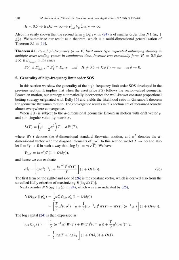
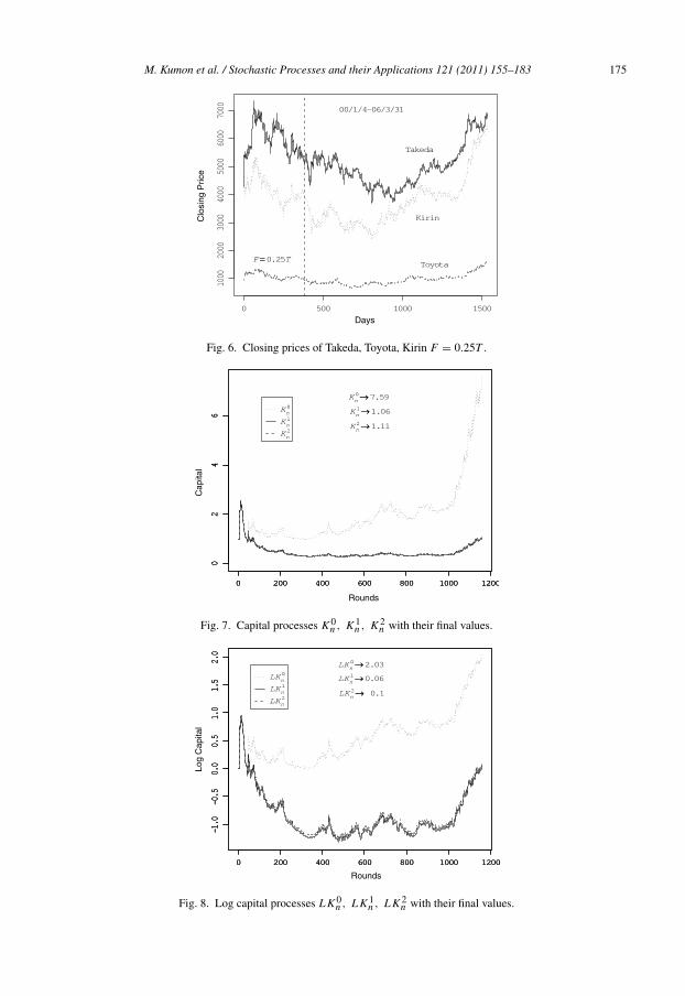
Figs. 1–5 and 6–10 exhibit the cases of three items Takeda, Toyota, Kirin with F = 0.17Tand F = 0.25T , respectively. The notations in the figures are as follows and their final values atthe end of round N are indicated in the figures.

K 0n = K∗

n = exp(nD(gn ‖ g∗n)), K 1

n = K∗n, K 2

n =K∗

n√

[In],

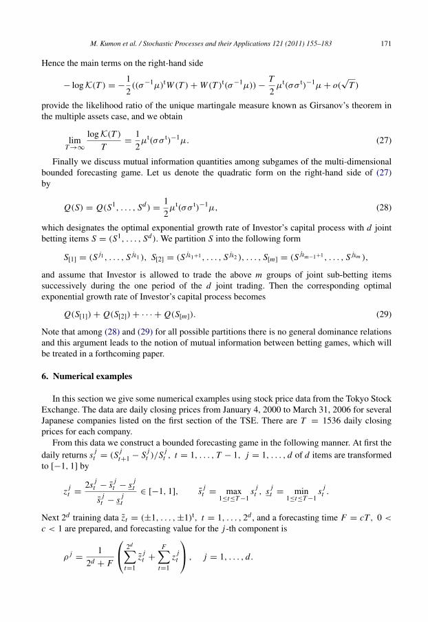
L K 0n = log K∗

n = nD(gn ‖ g∗n), L K 1

n = log K∗n,

L K 2n = nD(gn ‖ g∗

n) −12

log [In],

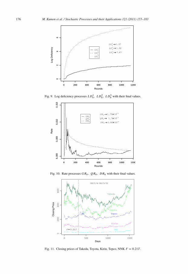
L D1n = log K∗

n − log K∗n, L D2

n =12

log [In], L D3n =

32

log n,

G Rn = D(gn ‖ g∗n), Q Rn =

12

x tn V ∗−1

n xn, DRn =log [In]

2n.

As suggested in Section 3.4, K 1n and K 2

n , L K 1n and L K 2

n , L D1n and L D2

n are almost overlaid inthe figures. We can also see that the actual log deficiency L D1

n or L D2n is far less than L D3 which

is the typical log deficiency in the case of finite items such as in the horse race game. FurthermoreFigs. 5, 10 show that the deficiency rate process DRn gives the precise convergence border ratefor the growth rate process G Rn or its approximated quadratic rate process Q Rn .

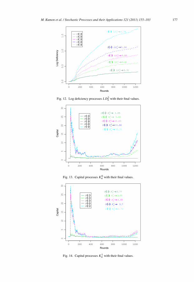
Figs. 11–16 illustrate the cases of composite games

Game(1) ⊂ Game(2) ⊂ Game(3) ⊂ Game(4) ⊂ Game(5)

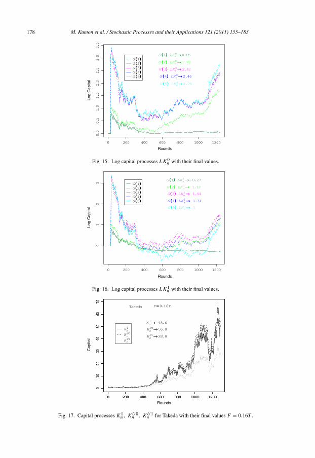
with five items 1. Takeda, 2. Toyota, 3. Kirin, 4. Tepco, 5. NNK in this order. As expected thefollowing trade-off can be seen in the figures.

L K 0n : G(1) < G(2) < G(3) < G(4) < G(5),

L D2n : G(1) < G(2) < G(3) < G(4) < G(5),

L K 1n : G(1) < G(5) < G(2) < G(4) < G(3).

Hence the choice of the three items 1. Takeda, 2. Toyota, 3. Kirin is the most profitable one inthe above composite games.

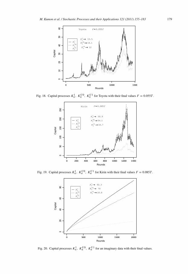
Figs. 17–20 compare the sequential optimizing strategy with the universal portfolio for oneitem Takeda, Toyota, Kirin, an imaginary data, respectively. The universal portfolio in its simplestform with one item can be performed in the following way.

Divide the closed interval A = α ∈ R | 1 + αx ≥ 0, ∀x ∈ D of prudent strategiesinto disjoint subintervals A1, . . . , AM . Then for the m-th account Am with the initial capitalK(m)

0 = 1/M , Skeptic continues the game with constant betting ratio αm ∈ Am, m = 1, . . . , M .

His capital at the end of round n is expressed as KUn =

∑Mm=1 K(m)

n . The figures are the caseswith M = 100 and the notations are

K U0n = KU

n without the training data −1, 1,

K U1n = KU

n with the training data −1, 1.


Clo

sing

Pric

e

Days

Fig. 1. Closing prices of Takeda, Toyota, Kirin F = 0.17T .

Cap

ital

Rounds

Fig. 2. Capital processes K 0n , K 1

n , K 2n with their final values.

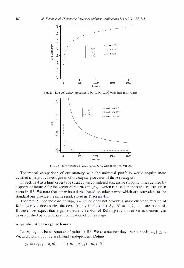
Figs. 20–22 show the case of an imaginary data given by

x−1 = −1, x0 = 1, xn =1

n + 1, n = 1, . . . , 2000.

In this case L K 1n ∼ a log n −c, 0 < a < 1, c > 0, which contrasts with the case of coin-tossing

game L K 1n ∼ nD(xn ‖ ρ) −

12 log n.

Figs. 17–20 suggest that there is no general superiority between the sequential optimizingstrategy and the universal portfolio.

7. Discussion

In this paper we proposed a sequential optimizing strategy in a multi-dimensional boundedforecasting game and showed that it is very flexible. From a theoretical viewpoint it allowed usto prove a generalized form of the strong law of large numbers. From a practical viewpoint thestrategy is easy to implement even in high dimensions and its performance is competitive againstthe universal portfolio.


Log

Cap

ital

Rounds

Fig. 3. Log capital processes L K 0n , L K 1

n , L K 2n with their final values.

Log

Def

icie

ncy

Rounds

Fig. 4. Log deficiency processes L D1n , L D2

n , L D3n with their final values.

Rat

e

Rounds

Fig. 5. Rate processes G Rn , Q Rn , DRn with their final values.


Clo

sing

Pric

e

Days

Fig. 6. Closing prices of Takeda, Toyota, Kirin F = 0.25T .

Cap

ital

Rounds

Fig. 7. Capital processes K 0n , K 1

n , K 2n with their final values.

Log

Cap

ital

Rounds

Fig. 8. Log capital processes L K 0n , L K 1

n , L K 2n with their final values.


Log

Def

icie

ncy

Rounds



Rat

e

Rounds


Clo

sing

Pric

e

Days

Fig. 11. Closing prices of Takeda, Toyota, Kirin, Tepco, NNK F = 0.21T .


Log

Def

icie

ncy

Rounds

Fig. 12. Log deficiency processes L D2n with their final values.

Cap

ital

Rounds

Fig. 13. Capital processes K 0n with their final values.

Cap

ital

Rounds

Fig. 14. Capital processes K 1n with their final values.


Log

Cap

ital

Rounds

Fig. 15. Log capital processes L K 0n with their final values.

Log

Cap

ital

Rounds

Fig. 16. Log capital processes L K 1n with their final values.

Cap

ital

Rounds

Fig. 17. Capital processes K 1n , K U0

n , K U1n for Takeda with their final values F = 0.16T .


Cap

ital

Rounds


n , K U1n for Toyota with their final values F = 0.055T .

Cap

ital

Rounds


n , K U1n for Kirin with their final values F = 0.085T .

Cap

ital

Rounds


n , K U1n for an imaginary data with their final values.


Log

Def

icie

ncy

Rounds



Rat

e

Rounds


Theoretical comparison of our strategy with the universal portfolio would require moredetailed asymptotic investigation of the capital processes of these strategies.

In Section 4 as a limit order type strategy we considered successive stopping times defined bya sphere of radius δ for the vector of returns (cf. (23)), which is based on the standard Euclideannorm in Rd . We note that other boundaries based on other norms which are equivalent to thestandard one provide the same result stated in Theorem 4.1.

Theorem 2.1 for the case of supN VN < ∞ does not provide a game-theoretic version ofKolmogorov’s three series theorem. It only implies that SN , N = 1, 2, . . . , are bounded.However we expect that a game-theoretic version of Kolmogorov’s three series theorem canbe established by appropriate modification of our strategy.

Appendix. A convergence lemma

Let u1, u2, . . . be a sequence of points in Rd . We assume that they are bounded: ‖un‖ ≤ 1,∀n, and that u1, . . . , ud are linearly independent. Define

yn = (u1ut1 + u2ut

2 + · · · + un−1utn−1)

−1un ∈ Rd .


Then we have the following lemma. It is trivial for d = 1, but for d > 1 we need a carefulargument.

Lemma A.1.

yn → 0, (n → ∞).

Proof. We first show that yn is bounded. Let λmin,d > 0 denote the minimum eigenvalue ofu1ut

1 + · · · + udutd . Then all the eigenvalues of u1ut

1 + · · · + unutn , n ≥ d, are greater than or

equal to λmin,d . Then all the eigenvalues of (u1ut1 +· · ·+unut

n)−2 are less than or equal to λ−2min,d .

Hence

‖yn‖2

≤ λ−2min,d‖un‖

2 (30)

and yn , n = 1, 2, . . . , are bounded.Now we argue by contradiction. Suppose that yn , n = 1, 2, . . . , do not converge to zero.

Then there exists a subsequence nk , k = 1, 2, . . . such that ynk → a = 0, (k → ∞). In view of(30), if unk → 0 then ynk → 0, which is a contradiction. Therefore unk , k = 1, 2, . . . , do notconverge to 0. Then there exists a further subsequence nk ⊂ nk such that unk → b = 0. Thenynk → a, unk → b. Consider

(u1ut1 + · · · + unk−1ut

nk−1)ynk = unk .

Then

(u1ut1 + · · · + unk−1ut

nk−1)ynk → b.

Multiplying by ytnk

from the left we have

ytnk

(u1ut1 + · · · + unk−1ut

nk−1)ynk = ytnk

unk → atb.

Now the left-hand side is written as

(ytnk

u1)2+ · · · + (yt

nkunk−1)

2.

Note that for sufficiently large k, k′, (ytnk

unk′)2 are all close to (bta)2. Since we have infinitely

many such terms, the left-hand side diverges to ∞ if bta = 0. This contradicts the fact that theright-hand side converges to a finite value. Therefore bta = 0. But then

lim inf(ytnk

u1)2+ · · · + (yt

nkunk−1)

2≥ (yt

nku1)

2+ · · · + (yt

nkud)2

→ (atu1)2+ · · · + (atud)2 > 0,

which is again a contradiction.

We also present the following corollary of the above lemma.

Corollary A.1. With the same notation and conditions as in Lemma 3.1

yn = (u1ut1 + u2ut

2 + · · · + un−1utn−1)

−1/2un → 0, (n → ∞).

This corollary follows easily from the fact that ‖yn‖2

= utn yn and un is bounded.

Based on the above corollary we give a proof of Lemma 3.1. Before going into the proof, wesummarize some facts on matrix inequalities. For a symmetric matrix A, let A > 0 mean thatA is positive definite. If A ≥ B > 0, then B−1

≥ A−1 > 0 (Lemma 4.2 of [2]). Note thatA ≥ B ≥ 0 does not imply A2

≥ B2 (e.g. Chapter 1 of [20]), which complicates our proof.


Proof of Lemma 3.1. By the definition of C1 in (15) we have

V0,n−1(α∗

n−1, α∗n) ≥

1

C21

V0,n−1(0, 0),

where V0,n−1(0, 0) =∑n

i=−n0+1 xi x ti is positive definite because of the training data. Write

1α∗n = V0,n−1(α

∗

n−1, α∗n)−1/2V0,n−1(α

∗

n−1, α∗n)−1/2xn(α∗

n−1).

Then

‖1α∗n‖

2≤

xn(α∗n)tV0,n−1(α

∗

n−1, α∗n)−1xn(α∗

n)

λmin,0,n−1(α∗

n−1, α∗n)

,

where λmin,0,n−1(α∗

n−1, α∗n) is the minimum eigenvalue of V0,n−1(α

∗

n−1, α∗n). Let λmin,0,0 denote

the minimum eigenvalue of V0,0. Then λmin,0,n−1(α∗

n−1, α∗n) ≥ λmin,0,0/C2

1 for all n ≥ 1 and

‖1α∗n‖

2≤

C21

λmin,0,0xn(α∗

n)tV0,n−1(α∗

n−1, α∗n)−1xn(α∗

n).

For n ≥ 1, 1 + α∗n · xn ≥ ϵ0. Hence

‖1α∗n‖

2≤

C21

ϵ20λmin,0,0

x tn V0,n−1(α

∗

n−1, α∗n)−1xn ≤

C41

ϵ20λmin,0,0

x tn V0,n−1(0, 0)−1xn .

The right-hand side converges to 0 by Corollary A.1.

References

[1] T.W. Anderson, An Introduction to Multivariate Statistical Analysis, 3rd ed., Wiley, Hoboken, New Jersey, 2003.[2] T.W. Anderson, A. Takemura, A new proof of admissibility of tests in the multivariate analysis of variance, Journal

of Multivariate Analysis 12 (1982) 457–478.[3] Thomas M. Cover, Universal portfolios, Mathematical Finance 1 (1) (1991) 1–29.[4] Thomas M. Cover, E. Ordentlich, Universal portfolios with side information, IEEE Transactions on Information

Theory IT-42 (1996) 348–363.[5] Thomas M. Cover, Joy A. Thomas, Elements of Information Theory, 2nd ed., Wiley, New York, 2006.[6] John L. Kelly, A new interpretation of information rate, Bell System Technical Journal 35 (1956) 917–26.[7] Masayuki Kumon, Akimichi Takemura, On a simple strategy weakly forcing the strong law of large numbers in the

bounded forecasting game, Annals of the Institute of Statistical Mathematics 60 (2008) 801–812.[8] Masayuki Kumon, Akimichi Takemura, Kei Takeuchi, Capital process and optimality properties of a Bayesian

Skeptic in coin-tossing games, Stochastic Analysis and Applications 26 (2008) 1161–1180.[9] E. Ordentlich, Thomas M. Cover, The cost of achieving the best portfolio in hindsight, Mathematics of Operations

Research 23 (4) (1998) 960–982.[10] Glenn Shafer, Vladimir Vovk, Probability and Finance: It’s Only a Game!, Wiley, New York, 2001.[11] Albert N. Shiryaev, Probability, second ed., Springer, New York, 1996.[12] William F. Stout, A martingale analog of Kolmogorov’s law of the iterated logarithm, Zeitschrift fur

Wahrscheinlichkeitstheorie und Verwandte Gebiete 15 (1970) 279–290.[13] Kei Takeuchi, Masayuki Kumon, Akimichi Takemura, A new formulation of asset trading games in continuous time

with essential forcing of variation exponent, Bernoulli 15 (2009) 1243–1258.[14] Kei Takeuchi, Masayuki Kumon, Akimichi Takemura, Multistep Bayesian strategy in coin-tossing games and its

application to asset trading games in continuous time, Stochastic Analysis and Applications 28 (2010) 842–861.[15] R.J. Tomkins, A law of the iterated logarithm for martingales, Zeitschrift fur Wahrscheinlichkeitstheorie und

Verwandte Gebiete 33 (1975) 65–68.[16] Vladimir Vovk, Continuous-time trading and the emergence of randomness, Stochastics 81 (2009) 455–466.[17] Vladimir Vovk, Continuous-time trading and the emergence of volatility, Electronic Communications in Probability

13 (2008) 319–324.


[18] Vladimir Vovk, Continuous-time trading and the emergence of probability. arXiv:0904.4364v1, 2009.[19] Vladimir Vovk, Rough paths in idealized financial markets. arXiv:1005.0279v1, 2010.[20] Xingzhi Zhan, Matrix Inequalities, Springer, Berlin, 2002.

http://arxiv.org/0904.4364v1

http://arxiv.org/1005.0279v1

sequential optimizing strategy in multi-dimensional bounded forecasting games

Documents