sequential innovation, patents, and imitation - home |...

RAND Journal of EconomicsVol. 40, No. 4, Winter 2009pp. 611–635

Sequential innovation, patents, and imitation

James Bessen∗and

Eric Maskin∗∗

We argue that when innovation is “sequential” (so that each successive invention builds inan essential way on its predecessors) and “complementary” (so that each potential innovatortakes a different research line), patent protection is not as useful for encouraging innovation asin a static setting. Indeed, society and even inventors themselves may be better off without suchprotection. Furthermore, an inventor’s prospective profit may actually be enhanced by competitionand imitation. Our sequential model of innovation appears to explain evidence from a naturalexperiment in the software industry.

1. Introduction

� The standard economic rationale for patents is to protect inventors from imitation andthereby give them the incentive to incur the cost of innovation. Conventional wisdom holds that,unless would-be competitors are restrained from imitating an invention, the inventor may not reapenough profit to cover that cost. Thus, even if the social benefit of invention exceeds the cost, thepotential innovator without patent protection may decide against innovating altogether.1

Yet interestingly, some of the most innovative industries of the last forty years—software,computers, and semiconductors—have historically had weak patent protection and have expe-rienced rapid imitation of their products.2 Defenders of patents may counter that, had stronger

∗Boston University School of Law and Research on Innovation; [email protected].∗∗Institute for Advanced Study and Princeton University; [email protected] thank Stefan Behringer, Lee Branstetter, Daniel Chen, Iain Cockburn, Partha Dasgupta, Nancy Gallini, AlfonsoGambardella, Bronwyn Hall, Adam Jaffe, Lawrence Lessig, David Levine, Suzanne Scotchmer, Jean Tirole, MichaelWhinston, two referees, the editor Joseph Harrington, and participants at many seminars and conferences for helpfulcomments. We gratefully acknowledge research support from the NSF.

1 This is not the only justification for patents. Indeed, we will emphasize a different, although related, rationalein Section 2. But, together with the spillover benefit that derives from the patent system’s disclosure requirements, itconstitutes the traditional justification.

2 Software was routinely excluded from patent protection in the United States until a series of court decisionsin the mid-1980s and 1990s. Semiconductor and computer patent enforcement was quite uneven until the organizationof the Federal Circuit Court in 1982. Both areas contend with substantial problems of prior art (Aharonian, 1992),and some experts argue that up to 90% of semiconductor patents are not truly novel and therefore invalid (Taylor andSilberston, 1973). These problems make consistent enforcement difficult and patents in these fields are much more likelyto be litigated (Bessen and Meurer, 2008). Surveys of managers in semiconductors and computers typically report thatpatents only weakly protect innovation. Levin et al. (1987) found that patents were rated weak at protecting the returns

Copyright C© 2009, RAND. 611

612 / THE RAND JOURNAL OF ECONOMICS

intellectual property rights been available, these industries would have been even more dynamic.But we will argue that there is reason to think otherwise.

In fact, the software industry in the United States was subjected to a revealing naturalexperiment in the 1980s and 1990s. Through a sequence of court decisions, patent protection forcomputer programs was significantly strengthened. Evidence suggests that, far from unleashinga flurry of new innovative activity, the firms that acquired most of these patents actually reducedtheir R&D spending relative to sales (Bessen and Hunt, 2004).3

We maintain, furthermore, that there is nothing paradoxical about this outcome. For industrieslike software or computers, theory suggests that imitation may promote innovation and thatstrong patents (long-lived patents of broad scope) might actually inhibit it. Society and even theinnovating firms themselves could well be served if intellectual property protection were morelimited in such industries. Moreover, these firms might genuinely welcome competition and theprospect of being imitated.4

This is, we argue, because these are industries in which innovation is both sequential andcomplementary. By “sequential,” we mean that each successive invention builds on the precedingone, in the way that the Lotus 1-2-3 spreadsheet built on VisiCalc, and Microsoft’s Excel built onLotus. And by “complementary,” we mean that each potential innovator takes a different researchline and thereby enhances the overall probability that a particular goal is reached within a giventime. Undoubtedly, the many different approaches taken to voice-recognition software hastenedthe availability of commercially viable packages.

Imitation of a discovery can be socially desirable in a world of sequential and complementaryinnovation because it helps the imitator develop further inventions. And because the imitator mayhave valuable ideas not available to the original discoverer, the overall pace of innovation maythereby be enhanced. In fact, in a sequential setting, the inventor himself could be better off ifothers imitate and compete against him. Although imitation reduces the profit from his currentdiscovery, it raises the probability of follow-on innovations, which improve his future profit. Ofcourse, some form of protection would be essential for promoting innovation, even in a sequentialsetting, if there were no cost to entry and no limit to how quickly imitation could take place: inthat case, imitators could immediately stream in whenever a new discovery was made, drivingthe inventor’s revenues to zero. Throughout the article, however, we assume that entry requiresinvestment in specialized capital, human or otherwise. Alternatively, we could assume that evenif setup costs do not deter would-be imitators from entering, entry does not occur instantly, andso the original innovator has at least a temporary first-mover advantage. The ability of firms togenerate positive (although possibly reduced) revenues when imitated accords well with empiricalevidence for high-technology industries.5

to innovation, far behind the protection gained from lead time and learning-curve advantages. Patents in electronicsindustries were estimated to increase initiation costs by only 7% (Mansfield, Schwartz, and Wagner, 1981) or 7–15%(Levin et al., 1987). Taylor and Silberston (1973) found that little R&D was undertaken to exploit patent rights. Asone might expect, diffusion and imitation are rampant in these industries. Tilton (1971) estimated the time from initialdiscovery to commercial imitation in Japanese semiconductors to be just over one year in the 1960s.

3 As Sakakibara and Branstetter (2001) show, a similar phenomenon occurred in Japan. Starting in the late 1980s,the Japanese patent system was significantly strengthened. However, Sakakibara and Branstetter argue that there was noconcomitant increase in R&D or innovation.

4 Here are some examples in which firms have appeared to encourage imitation: When IBM announced its firstpersonal computer in 1981, Apple Computer, then the industry leader, responded with full-page newspaper ads headed,“Welcome, IBM. Seriously.” Adobe put Postscript and PDF format in the public domain, inviting other firms to be directcompetitors for some Adobe products. Cisco (and other companies) regularly contribute patented technology to industrystandards bodies, allowing any entrant to produce competing products. Finally, IBM and several other firms have recentlydonated a number of patents for free use by open source developers. The stated reason for this donation was to build theoverall “ecosystem.” See also Keely (2005).

5 For example, consider that (1) the software industry is highly segmented (see Mowery, 1996), suggesting thatspecialized knowledge prevents a firm that is successful in one segment to move to another and (2) survey data from theelectronics and computer industries (see Levin et al., 1987) indicate that “lead-time advantage” and “moving down thelearning curve quickly” provide more effective protection than patents.

C© RAND 2009.

BESSEN AND MASKIN / 613

But whether or not an inventor without patent protection himself gains from being imitated,he is more likely (as we will show in one of our main results, Proposition 6) to be able to cover hiscost of innovation in a sequential than a static environment, provided that it is socially desirablefor him to incur this cost. This conclusion weakens the justification for intellectual propertyprotection, such as patents, in sequential settings. Indeed, as we establish in Proposition 7, patentsmay actually reduce welfare: by blocking imitation, they may interfere with further innovation.Of course, patent defenders have a counterargument to this criticism: if a patent threatens toimpede valuable follow-on innovative activity, the patent holder should have the incentive togrant licenses to those conducting the activity (thereby allowing innovation to occur). After all,if the follow-on R&D is worthwhile, she could share in its value by a suitably chosen licensingfee/royalty, thereby increasing her own profit (or so the argument goes).

A serious problem with this counterargument, however, is that it ignores the likely asymmetrybetween potential innovators in information about future profits. There is a large literature onpatent licensing, but to our knowledge it has not addressed this asymmetry.6 In our setting, ifa patent holder is not as well-informed about a rival’s potential future profits as the rival ishimself, she may have difficulty setting a mutually profitable license fee, and so, as Proposition 7shows, licensing may fail,7 thereby jeopardizing subsequent innovation (of course, informationalasymmetries about current profits, which we rule out for convenience, would only aggravate thisproblem).

In short, when innovation is sequential and complementary, standard conclusions aboutpatents and imitation may get turned on their heads. Imitation becomes a spur to innovation,whereas strong patents become an impediment.

Sequential innovation has also been studied by Scotchmer (1991, 1996), Scotchmer andGreen (1990), Green and Scotchmer (1996), and Chang (1995) for the case of a single follow-oninnovation. Hunt (2004), O’Donoghue (1998), and O’Donoghue, Scotchmer, and Thisse (1998)study a single invention with an infinite sequence of quality improvements. We depart from thisliterature primarily in our model of competition. In our analysis, different firms’ products at anygiven stage differ from one another.8 That is, imitators do not produce direct “knockoffs,” butrather differentiated products. This sort of differentiation is widely observed and is, of course,the subject of its own literature. But our main point here is that the different R&D paths behindthese products permit innovative complementarities. Imitation then increases the “biodiversity”of the technology (see footnote 4), improving prospects for future innovation.

We proceed as follows. In Section 2, we introduce a static (nonsequential) model that, weclaim, underlies the traditional justification for patents. We emphasize the point that, besideshelping an inventor to cover his costs, an important role of patents is to encourage innovativeactivity on the part of others who would otherwise be inclined merely to imitate. Analytically, weshow that (i) without patents, the equilibrium level of innovative activity is less than or equal to theoptimum, and (ii) with patents, the level is greater than or equal to the optimum (Proposition 1).Despite the potential welfare ambiguity this result suggests, we argue that, on balance, patentsare better than no patents: provided that the upper tail of the distribution of innovation valuesis sufficiently thick (which, we argue, is the empirically relevant case), expected welfare withpatent protection exceeds that without it (Proposition 2). Not surprisingly, inventors themselves

6 Some articles on patent licensing consider, as we do, the issue of licensing to one’s own competitiors, includingKatz and Shapiro (1985, 1986), Gallini (1984), and Gallini and Winter (1985). In these articles, however, the social lossfrom failure to license tends to derive from higher costs (because of decreasing returns to scale in monopoly production)and high consumer prices, rather than from reduced innovation.

7 Although this phenomenon does not appear to have been analyzed in the existing patents literature, a closelyrelated phenomenon has been examined in the literature on common pool resources such as oil reservoirs. As Wigginsand Libecap (1985) discuss, oil well owners can realize larger total profits if they contract to jointly manage production.But contract negotiations typically involve asymmetric information about future profits. The empirical evidence showsthat contracting over oil production typically fails, despite industry-specific regulation designed to encourage it. In onecase, only 12 out of 3,000 oil fields were completely covered by joint production agreements.

8 This feature also figures prominently in the models in Dasgupta and Maskin (1987) and Tandon (1983).

C© RAND 2009.


are also better off with patent protection (Proposition 3). We also note that, in this static model,competition unambiguously diminishes the payoff of a prospective inventor (Proposition 4).

In Section 3, we modify the model to accommodate a potentially infinite sequence ofinventions, each building on its predecessor. Because R&D now serves to raise the probability notonly of the current invention but of future ones too, the equilibrium level of R&D will generally behigher than in the static model. However we show that the equilibrium level of innovative activitywhen there is no patent protection is still generally less than the optimum (Proposition 5). Evenso, we establish that the gap between the equilibrium level and the optimal level is smaller thanin the static model. Thus, equilibrium without patents is more nearly optimal with sequentialthan with static innovation (Proposition 6), implying that the case for intellectual propertyprotection is correspondingly weaker. Indeed, under the same hypotheses for which we derivedthe opposite conclusion in the static model, the levels of social welfare and innovation whenthere is patent protection are actually lower on average than when there is not, (Proposition 7).Finally, we establish that, under somewhat more stringent assumptions, inventors themselvesbenefit from the absence of patent protection (Proposition 8) and may actually gain from beingimitated, whether or not there is patent protection (Proposition 9), again in contrast to the staticmodel. Most proofs are relegated to Appendix B.

2. The static model

� We consider an industry consisting of two (ex ante symmetric) firms.9 Each firmchooses whether or not to undertake R&D10 to discover and develop an invention with(social) value v,11 where v is known publicly and drawn ex ante from distribution withc.d.f . F(v). We suppose that a firm’s cost C of R&D is a random variable: with probabilityq, C = c, and with probability 1 − q, C = 0.12 A firm learns the realization of C before itdecides whether to undertake R&D, but this information is private. Realizations are (statistically)independent across the two firms.

If a single firm undertakes R&D, the probability of successful innovation is p1.13 If bothfirms do R&D, the probability that at least one of them will succeed is p2. We model the ideaof complementarity—that having different firms pursue the same technological goal raises theprobability that someone will succeed—by supposing that p2 > p1; each firm’s probability ofsuccess is only p1,14 but because their research strategies are not perfectly positively correlated,the overall probability of success is higher. Of course, we must also have p2 < 2p1, that is,

p1 < p2 < 2p1, (1)

because, at best, the two firms’ research strategies will be perfectly negatively correlated (inwhich case, p2 = 2p1).

We first consider the socially efficient R&D decisions for the two firms, that is, the decisionsthat a planner maximizing social welfare would direct them to take. Actually, because we

9 Limiting the model to two firms in particular is a matter only of expositional convenience; all our results extendto any other finite number of firms. However, by assuming the number of firms is finite, we are implicitly supposing thatthere is a limit on how many firms are able to imitate a given invention, implying that an innovator’s revenue need not bedriven to zero in equilibrium. As we note above (and in footnote 5), we could alternatively assume that imitation takestime. Either way, it is important for our argument that, even without patent protection, the inventor be able to obtain somerevenue from an invention.

10 Throughout this article, a firm’s R&D decision is a binary choice: to do it or not to do it. But all our resultsgeneralize to the case where the firm can vary the intensity of its R&D effort.

11 There is no additional social value that accrues if both firms discover the innovation.12 We have chosen the smaller realization to be zero merely for analytic convenience; all our results hold with a

positive lower cost.13 Our framework in this section is static, but if it were viewed as the reduced form of a dynamic setting, then p1

could alternatively be interpreted as the discount factor corresponding to the time lag to innovation.14 That is, we rule out externalities in which one firm’s R&D raises the other’s chance of success. Of course, such

spillovers are interesting and, in practice, important. But here they would serve only to strengthen our findings.

C© RAND 2009.


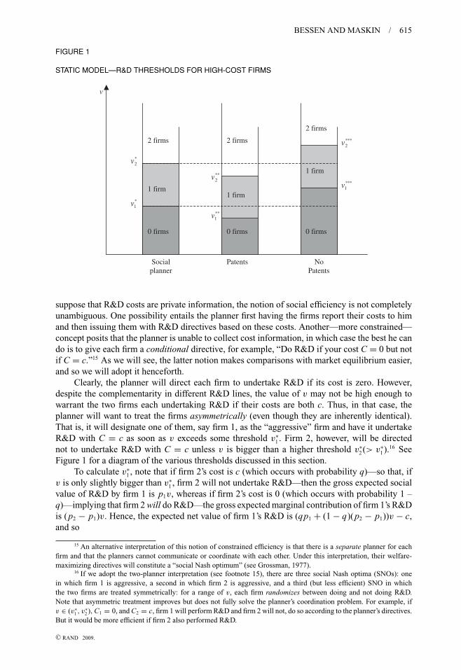
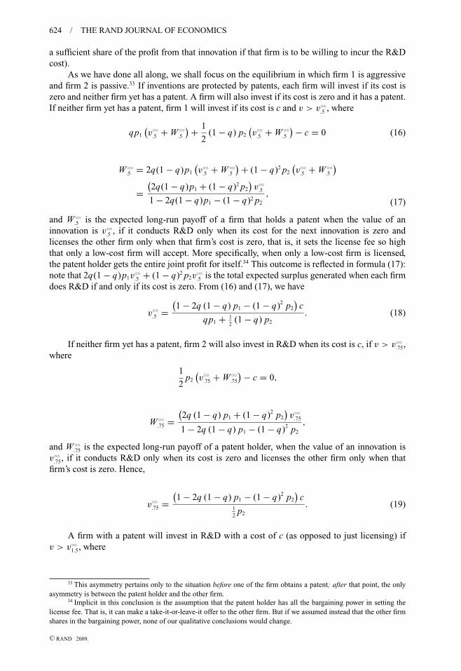
FIGURE 1

STATIC MODEL—R&D THRESHOLDS FOR HIGH-COST FIRMS

0 firms

1 firm

2 firms

0 firms

1 firm

2 firms

0 firms

1 firm

2 firms

Socialplanner

Patents NoPatents

∗1v

∗2v

∗∗1v

∗∗2v

∗∗∗1v

∗∗∗2v

v

suppose that R&D costs are private information, the notion of social efficiency is not completelyunambiguous. One possibility entails the planner first having the firms report their costs to himand then issuing them with R&D directives based on these costs. Another—more constrained—concept posits that the planner is unable to collect cost information, in which case the best he cando is to give each firm a conditional directive, for example, “Do R&D if your cost C = 0 but notif C = c.”15 As we will see, the latter notion makes comparisons with market equilibrium easier,and so we will adopt it henceforth.

Clearly, the planner will direct each firm to undertake R&D if its cost is zero. However,despite the complementarity in different R&D lines, the value of v may not be high enough towarrant the two firms each undertaking R&D if their costs are both c. Thus, in that case, theplanner will want to treat the firms asymmetrically (even though they are inherently identical).That is, it will designate one of them, say firm 1, as the “aggressive” firm and have it undertakeR&D with C = c as soon as v exceeds some threshold v∗

1 . Firm 2, however, will be directednot to undertake R&D with C = c unless v is bigger than a higher threshold v∗

2 (> v∗1 ).16 See

Figure 1 for a diagram of the various thresholds discussed in this section.To calculate v∗

1 , note that if firm 2’s cost is c (which occurs with probability q)—so that, ifv is only slightly bigger than v∗

1 , firm 2 will not undertake R&D—then the gross expected socialvalue of R&D by firm 1 is p1v, whereas if firm 2’s cost is 0 (which occurs with probability 1 –q)—implying that firm 2 will do R&D—the gross expected marginal contribution of firm 1’s R&Dis (p2 − p1)v. Hence, the expected net value of firm 1’s R&D is (qp1 + (1 − q)(p2 − p1))v − c,and so

15 An alternative interpretation of this notion of constrained efficiency is that there is a separate planner for eachfirm and that the planners cannot communicate or coordinate with each other. Under this interpretation, their welfare-maximizing directives will constitute a “social Nash optimum” (see Grossman, 1977).

16 If we adopt the two-planner interpretation (see footnote 15), there are three social Nash optima (SNOs): onein which firm 1 is aggressive, a second in which firm 2 is aggressive, and a third (but less efficient) SNO in whichthe two firms are treated symmetrically: for a range of v, each firm randomizes between doing and not doing R&D.Note that asymmetric treatment improves but does not fully solve the planner’s coordination problem. For example, ifv ∈ (v∗

1 , v∗2 ), C1 = 0, and C2 = c, firm 1 will perform R&D and firm 2 will not, do so according to the planner’s directives.

But it would be more efficient if firm 2 also performed R&D.

C© RAND 2009.


(qp1 + (1 − q) (p2 − p1)) v∗1 − c = 0,

that is,

v∗1 = c

qp1 + (1 − q) (p2 − p1). (2)

Similarly, we have

(p2 − p1) v∗2 − c = 0,

that is,

v∗2 = c

p2 − p1

. (3)

Turning from this normative analysis, we next examine the nature of equilibrium when theinvention in question can be patented. We suppose that a firm with a patent can capture the fullsocial benefit v of the invention.17 If both firms undertake R&D, each has a probability 1

2p2 of

getting the patent.18

Corresponding to the three possible social Nash optima of the efficiency analysis (seefootnote 16), there are three possible equilibria when the invention is patentable: (i) one in whichfirm 1 is aggressive and firm 2 is passive, (ii) the mirror image, in which the firms’ roles arereversed, and (iii) a symmetric equilibrium in which, for a range of values of v, the firms bothrandomize between doing and not doing R&D. For comparison with the planner’s problem, wewill focus on (i), which is strictly more efficient than (iii)—of course, we could just as easily haveconcentrated on (ii)

In equilibrium (i), each firm will undertake R&D if its cost is zero—it has nothing to lose bydoing so. If v is not too big, then, from firm 1’s point of view, the probability that the other firmdoes R&D is 1 − q and the probability that it does not is q. Hence, firm 1 will undertake R&Dwith C = c if its expected revenue (qp1 + 1

2(1 − q)p2)v exceeds its cost c, that is, if v > v∗∗

1 ,where (

qp1 + 1

2(1 − q) p2

)v∗∗

1 − c = 0,

or

v∗∗1 = c

qp1 + 1

2(1 − q) p2

. (4)

As for firm 2, it will not undertake R&D with C = c unless v is sufficiently high for it tomake a profit even when firm 1 does R&D too. That is, v must exceed v∗∗

2 , where

1

2p2v

∗∗2 − c = 0,

or

v∗∗2 = 2c

p2

. (5)

17 This, of course, is a strong assumption. However, the incentive failures and monopoly inefficiencies that arisewhen it is not imposed are already well understood. The assumption is a simple way to abstract from these familiardistortions. It also accords with our approach of making suppositions favorable to patenting in order to draw strongerconclusions about patents’ failures in Section 3.

18 The total probability of discovery is p2, and each firm has a one-half chance of making it first. This gets at theidea that patents have breadth (so that a patent holder can block the implementation of other firms’ discoveries that aresimilar, but not identical, to its own). That is, only one firm can get a patent.

C© RAND 2009.


Finally, we investigate the nature of equilibrium when there is no patent protection. Weassume that, without patents, if either firm is successful in making the discovery, the other canimitate costlessly19 and that competition then drives each firm’s gross revenue down to a fractions(0 < s ≤ 1

2) of the total value v.20

Once again, there are three possible equilibria, and, as before, we will concentrate on the onein which firm 1 is aggressive and firm 2 is passive. In this equilibrium, either firm will undertakeR&D if its cost is zero. Firm 1 will undertake R&D with C = c if v > v∗∗∗

1 , where

(qsp1 + (1 − q) s (p2 − p1)) v∗∗∗1 − c = 0,

that is,

v∗∗∗1 = c

qsp1 + (1 − q) s (p2 − p1). (6)

Comparing (2) with (6), we see that v∗1 < v∗∗∗

1 . This inequality corresponds to the classic incentivefailure that the patent system is meant to address. When v∗

1 < v < v∗∗∗1 , firm 1 cannot make a profit

on its R&D investment without protection from imitation, despite the fact that such investmentwould be socially beneficial. A patent solves this problem by proscribing imitation. From (1),12

p2 > p2 − p1, and so from (2) and (4), v∗∗1 < v∗

1 . Hence, with the prospect of patent protection,firm 1 will be willing to undertake R&D investment, provided this is socially worthwhile.

But even in a setting where v > v∗∗∗1 —so that R&D is profitable despite imitation—patents

may well serve a useful purpose. This is because they can encourage several firms to go after thesame innovation, which may be beneficial because of complementarity. In the absence of patentprotection, firm 2 will earn expected profit

sp2v − c, (7)

if it decides to undertake R&D like firm 1. If, instead, it sits back and waits to imitate firm 1’sinvention, it can expect profit

sp1v. (8)

Hence, in equilibrium, it will invest in R&D only if (7) exceeds (8), that is, if v > v∗∗∗2 , where

s (p2 − p1) v∗∗∗2 − c = 0,

or

v∗∗∗2 = c

s (p2 − p1). (9)

But v∗2 < v∗∗∗

2 , and so if v lies between v∗2 and v∗∗∗

2 , we again have an incentive failure:although firm 1 will undertake R&D, firm 2 will merely imitate, despite the net social benefitfrom its investing too.

Here again patents come to the rescue. With the prospect of patent protection, firm 2 willundertake R&D provided that v > v∗∗

2 . So, from (1), (2), and (5), v∗∗2 < v∗

2 , implying that it willundertake R&D if such investment is socially desirable.

19 In reality, even imitations that are complete knockoffs may involve substantial expenses, but our assumption getsat the idea that such expenses will typically be dwarfed by the innovating firm’s R&D costs. Of course, some inventionsare so difficult to reverse-engineer that trade secrecy adequately protects against imitation. But such inventions are notlikely to be patented anyway, even if they could be, because of the patent system’s disclosure requirements. To studypotential shortcomings of the patent system, our focus in this article is on innovations that inventors would choose topatent if offered the opportunity.

20 By assuming symmetry here, we simplify the computations a bit but, perhaps more importantly, we arestrengthening the case for patents (if instead the innovating firm got the lion’s share of the profit from the discovery, thensafeguarding intellectual property would not matter as much). This will bolster our argument in Section 3, where we pointout why patent protection may be socially undesirable.

C© RAND 2009.


Patents, therefore, accomplish more than merely protecting inventors from imitation; theyencourage would-be imitators to invest in innovation themselves. Indeed, they create a risk ofoverinvestment in R&D: notice that v∗∗

1 is strictly less than v∗1 , and v∗∗

2 is strictly less than v∗2 .21

Overinvestment can come about because when a firm decides to undertake R&D, it increasesthe probability that the discovery will be made, but also diminishes the other firm’s chances ofgetting a patent. Because it doesn’t take this negative externality into account, it is overly inclinedto undertake R&D.

We summarize these results with the following proposition (see Figure 1 for a graphicalsummary):

Proposition 1. In the static model, the equilibrium level of R&D investment without patents isless than or equal to the social optimum. By contrast, the equilibrium level of R&D investmentwith patent protection is greater than or equal to the social optimum.

Observe that the possible overinvestment in R&D induced by patents could, in principle,be avoided if there were no complementarities of research across firms. Specifically, one couldimagine awarding a firm an “ex ante patent,” for example, the right to research and develop avaccine against a particular disease.22 Such protection would, of course, serve to prevent additionalfirms from attempting to develop the invention in question. But this would be efficient, providedthat the firm with the patent had the greatest chance for success (which could be ensured, forexample, by awarding the patent through an auction) and that the other firms would not enhancethe probability or speed of development, that is, provided that they conferred no complementarity.

But even with the possibility of overinvestment, there is an important sense in which a regimewith patents may be superior to one without them—if patents serve to encourage R&D projectswith large returns, then the benefits from these projects can more than offset the welfare lossesfrom overinvestment in more marginal projects. That is, despite potential welfare ambiguities,the standard economic doctrine that patents are a “good thing” does follow once we suppose theprobability of high returns is not too much lower than that of low returns (indeed, this is morethan just a theoretical hypothesis; see the empirical discussion in footnote 23).

To make this claim precise, imagine that the social (gross) value of innovation v is drawnfrom a distribution with twice-differentiable c.d.f. F(v) and that, for some k > 0 and v̄ > 0, thefollowing condition holds:

Upper Tail Condition :d2 F(v)

dv2≥ −k for all v ∈

[c

p1

, v̄

].

For v̄ sufficiently big and k sufficiently small, this condition ensures that the upper tail ofthe distribution does not fall off too quickly (the lower bound c

p1is chosen low enough so that the

Condition applies in all the Propositions below where it is invoked). The Pareto and lognormaldistributions, which are commonly found to fit distributions of returns to inventions and patentvalues in empirical research,23 meet this requirement for appropriately chosen parameters.24

(In Section 3, we shall offer another reason for invoking the Upper Tail Condition.) Wecan now state a formal justification for the standard economic doctrine favoring the patentsystem:

21 The possibility that patents can give rise to excessive spending on R&D is well known from the patent-raceliterature; see Dasgupta and Stiglitz (1980) and Loury (1979).

22 Wright (1983) and Shavell and Ypersele (2001) explore similar schemes.23 Early survey evidence suggested that the distribution of returns on patented inventions was highly skewed

(Sanders, Rossman, and Harris, 1958). Using patent renewal data from Europe, Pakes and Schankerman (1984) foundthat the values of low-value patents could be fit with a Pareto distribution. More recent research has assessed the value ofinventions in the upper tail by a variety of means and concluded that the distribution is fit well with a Pareto distributionfunction or a truncated lognormal distribution (only the upper tail of the lognormal distribution is observed); see Schererand Harhoff, 2000 and Silverberg and Verspagen, 2004.

24 This is established in Appendix A.

C© RAND 2009.


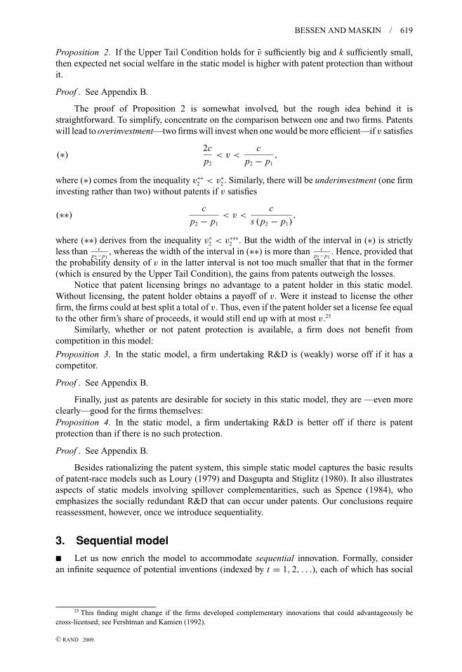
Proposition 2. If the Upper Tail Condition holds for v̄ sufficiently big and k sufficiently small,then expected net social welfare in the static model is higher with patent protection than withoutit.

Proof . See Appendix B.

The proof of Proposition 2 is somewhat involved, but the rough idea behind it isstraightforward. To simplify, concentrate on the comparison between one and two firms. Patentswill lead to overinvestment—two firms will invest when one would be more efficient—if v satisfies

(∗)2c

p2

< v <c

p2 − p1

,

where (∗) comes from the inequality v∗∗2 < v∗

2 . Similarly, there will be underinvestment (one firminvesting rather than two) without patents if v satisfies

(∗∗)c

p2 − p1

< v <c

s (p2 − p1),

where (∗∗) derives from the inequality v∗2 < v∗∗∗

2 . But the width of the interval in (∗) is strictlyless than c

p2−p1, whereas the width of the interval in (∗∗) is more than c

p2−p1. Hence, provided that

the probability density of v in the latter interval is not too much smaller that that in the former(which is ensured by the Upper Tail Condition), the gains from patents outweigh the losses.

Notice that patent licensing brings no advantage to a patent holder in this static model.Without licensing, the patent holder obtains a payoff of v. Were it instead to license the otherfirm, the firms could at best split a total of v. Thus, even if the patent holder set a license fee equalto the other firm’s share of proceeds, it would still end up with at most v.25

Similarly, whether or not patent protection is available, a firm does not benefit fromcompetition in this model:

Proposition 3. In the static model, a firm undertaking R&D is (weakly) worse off if it has acompetitor.


Finally, just as patents are desirable for society in this static model, they are —even moreclearly—good for the firms themselves:Proposition 4. In the static model, a firm undertaking R&D is better off if there is patentprotection than if there is no such protection.


Besides rationalizing the patent system, this simple static model captures the basic resultsof patent-race models such as Loury (1979) and Dasgupta and Stiglitz (1980). It also illustratesaspects of static models involving spillover complementarities, such as Spence (1984), whoemphasizes the socially redundant R&D that can occur under patents. Our conclusions requirereassessment, however, once we introduce sequentiality.

3. Sequential model

� Let us now enrich the model to accommodate sequential innovation. Formally, consideran infinite sequence of potential inventions (indexed by t = 1, 2, . . .), each of which has social

25 This finding might change if the firms developed complementary innovations that could advantageously becross-licensed; see Fershtman and Kamien (1992).

C© RAND 2009.


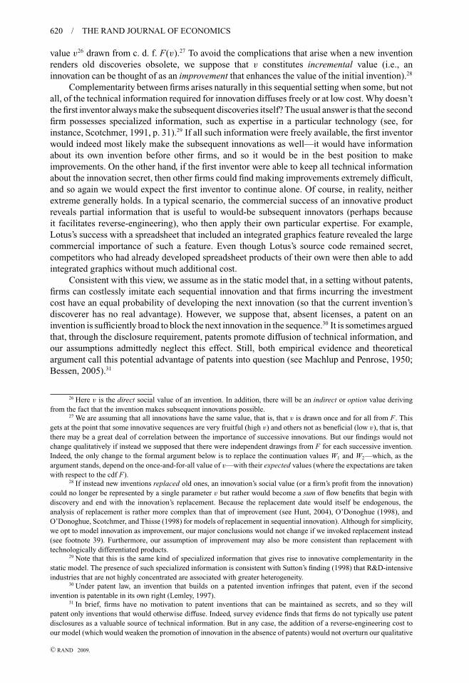
value v26 drawn from c. d. f. F(v).27 To avoid the complications that arise when a new inventionrenders old discoveries obsolete, we suppose that v constitutes incremental value (i.e., aninnovation can be thought of as an improvement that enhances the value of the initial invention).28

Complementarity between firms arises naturally in this sequential setting when some, but notall, of the technical information required for innovation diffuses freely or at low cost. Why doesn’tthe first inventor always make the subsequent discoveries itself? The usual answer is that the secondfirm possesses specialized information, such as expertise in a particular technology (see, forinstance, Scotchmer, 1991, p. 31).29 If all such information were freely available, the first inventorwould indeed most likely make the subsequent innovations as well—it would have informationabout its own invention before other firms, and so it would be in the best position to makeimprovements. On the other hand, if the first inventor were able to keep all technical informationabout the innovation secret, then other firms could find making improvements extremely difficult,and so again we would expect the first inventor to continue alone. Of course, in reality, neitherextreme generally holds. In a typical scenario, the commercial success of an innovative productreveals partial information that is useful to would-be subsequent innovators (perhaps becauseit facilitates reverse-engineering), who then apply their own particular expertise. For example,Lotus’s success with a spreadsheet that included an integrated graphics feature revealed the largecommercial importance of such a feature. Even though Lotus’s source code remained secret,competitors who had already developed spreadsheet products of their own were then able to addintegrated graphics without much additional cost.

Consistent with this view, we assume as in the static model that, in a setting without patents,firms can costlessly imitate each sequential innovation and that firms incurring the investmentcost have an equal probability of developing the next innovation (so that the current invention’sdiscoverer has no real advantage). However, we suppose that, absent licenses, a patent on aninvention is sufficiently broad to block the next innovation in the sequence.30 It is sometimes arguedthat, through the disclosure requirement, patents promote diffusion of technical information, andour assumptions admittedly neglect this effect. Still, both empirical evidence and theoreticalargument call this potential advantage of patents into question (see Machlup and Penrose, 1950;Bessen, 2005).31

26 Here v is the direct social value of an invention. In addition, there will be an indirect or option value derivingfrom the fact that the invention makes subsequent innovations possible.

27 We are assuming that all innovations have the same value, that is, that v is drawn once and for all from F. Thisgets at the point that some innovative sequences are very fruitful (high v) and others not as beneficial (low v), that is, thatthere may be a great deal of correlation between the importance of successive innovations. But our findings would notchange qualitatively if instead we supposed that there were independent drawings from F for each successive invention.Indeed, the only change to the formal argument below is to replace the continuation values W1 and W2—which, as theargument stands, depend on the once-and-for-all value of v—with their expected values (where the expectations are takenwith respect to the cdf F).

28 If instead new inventions replaced old ones, an innovation’s social value (or a firm’s profit from the innovation)could no longer be represented by a single parameter v but rather would become a sum of flow benefits that begin withdiscovery and end with the innovation’s replacement. Because the replacement date would itself be endogenous, theanalysis of replacement is rather more complex than that of improvement (see Hunt, 2004), O’Donoghue (1998), andO’Donoghue, Scotchmer, and Thisse (1998) for models of replacement in sequential innovation). Although for simplicity,we opt to model innovation as improvement, our major conclusions would not change if we invoked replacement instead(see footnote 39). Furthermore, our assumption of improvement may also be more consistent than replacement withtechnologically differentiated products.

29 Note that this is the same kind of specialized information that gives rise to innovative complementarity in thestatic model. The presence of such specialized information is consistent with Sutton’s finding (1998) that R&D-intensiveindustries that are not highly concentrated are associated with greater heterogeneity.

30 Under patent law, an invention that builds on a patented invention infringes that patent, even if the secondinvention is patentable in its own right (Lemley, 1997).

31 In brief, firms have no motivation to patent inventions that can be maintained as secrets, and so they willpatent only inventions that would otherwise diffuse. Indeed, survey evidence finds that firms do not typically use patentdisclosures as a valuable source of technical information. But in any case, the addition of a reverse-engineering cost toour model (which would weaken the promotion of innovation in the absence of patents) would not overturn our qualitative

C© RAND 2009.


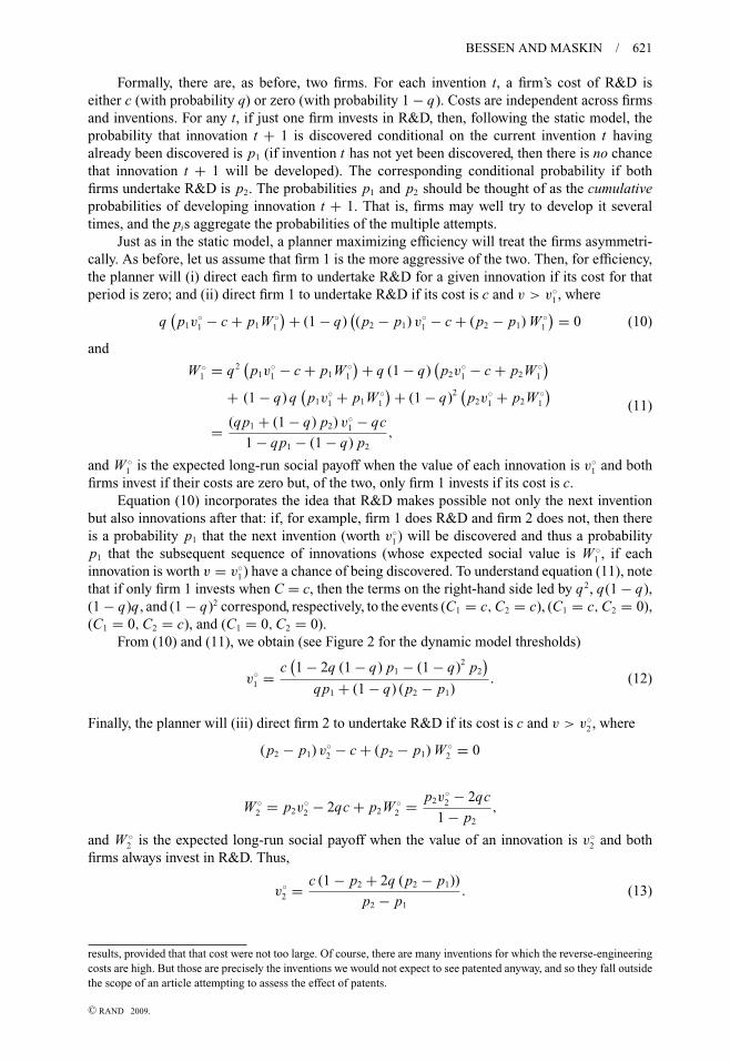
Formally, there are, as before, two firms. For each invention t, a firm’s cost of R&D iseither c (with probability q) or zero (with probability 1 − q). Costs are independent across firmsand inventions. For any t, if just one firm invests in R&D, then, following the static model, theprobability that innovation t + 1 is discovered conditional on the current invention t havingalready been discovered is p1 (if invention t has not yet been discovered, then there is no chancethat innovation t + 1 will be developed). The corresponding conditional probability if bothfirms undertake R&D is p2. The probabilities p1 and p2 should be thought of as the cumulativeprobabilities of developing innovation t + 1. That is, firms may well try to develop it severaltimes, and the pis aggregate the probabilities of the multiple attempts.

Just as in the static model, a planner maximizing efficiency will treat the firms asymmetri-cally. As before, let us assume that firm 1 is the more aggressive of the two. Then, for efficiency,the planner will (i) direct each firm to undertake R&D for a given innovation if its cost for thatperiod is zero; and (ii) direct firm 1 to undertake R&D if its cost is c and v > v◦

1 , where

q(

p1v◦1 − c + p1W ◦

1

) + (1 − q)((p2 − p1) v◦

1 − c + (p2 − p1) W ◦1

) = 0 (10)

and

W ◦1 = q2

(p1v

◦1 − c + p1W ◦

1

) + q (1 − q)(

p2v◦1 − c + p2W ◦

1

)+ (1 − q) q

(p1v

◦1 + p1W ◦

1

) + (1 − q)2(

p2v◦1 + p2W ◦

1

)= (qp1 + (1 − q) p2) v◦

1 − qc

1 − qp1 − (1 − q) p2

,

(11)

and W ◦1 is the expected long-run social payoff when the value of each innovation is v◦

1 and bothfirms invest if their costs are zero but, of the two, only firm 1 invests if its cost is c.

Equation (10) incorporates the idea that R&D makes possible not only the next inventionbut also innovations after that: if, for example, firm 1 does R&D and firm 2 does not, then thereis a probability p1 that the next invention (worth v◦

1) will be discovered and thus a probabilityp1 that the subsequent sequence of innovations (whose expected social value is W ◦

1 , if eachinnovation is worth v = v◦

1) have a chance of being discovered. To understand equation (11), notethat if only firm 1 invests when C = c, then the terms on the right-hand side led by q2, q(1 − q),(1 − q)q, and (1 − q)2 correspond, respectively, to the events (C1 = c, C2 = c), (C1 = c, C2 = 0),(C1 = 0, C2 = c), and (C1 = 0, C2 = 0).

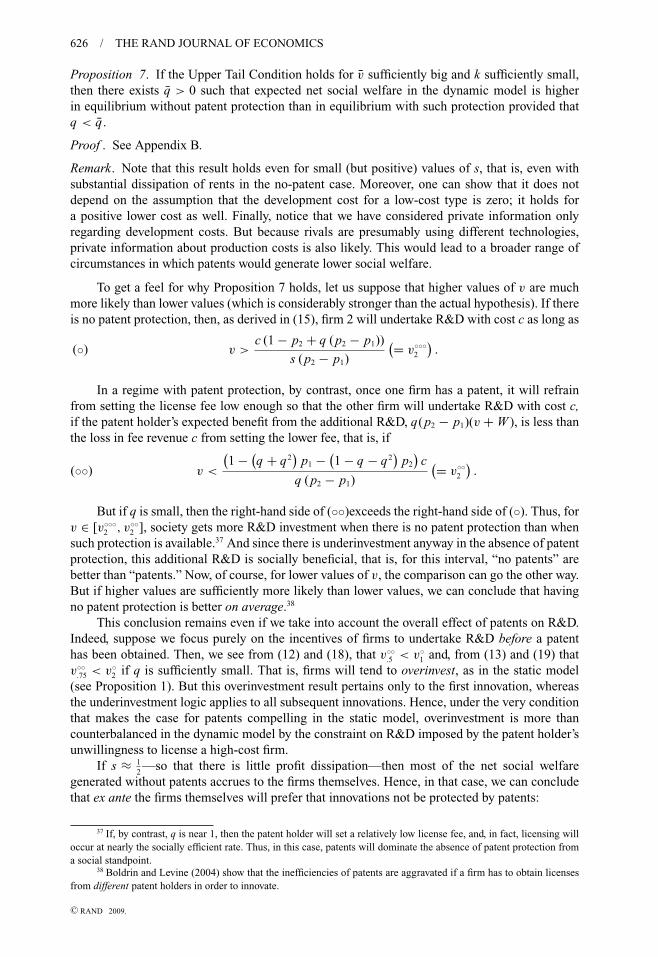
From (10) and (11), we obtain (see Figure 2 for the dynamic model thresholds)

v◦1 = c

(1 − 2q (1 − q) p1 − (1 − q)2 p2

)qp1 + (1 − q) (p2 − p1)

. (12)

Finally, the planner will (iii) direct firm 2 to undertake R&D if its cost is c and v > v◦2 , where

(p2 − p1) v◦2 − c + (p2 − p1) W ◦

2 = 0

W ◦2 = p2v

◦2 − 2qc + p2W ◦

2 = p2v◦2 − 2qc

1 − p2

,

and W ◦2 is the expected long-run social payoff when the value of an innovation is v◦

2 and bothfirms always invest in R&D. Thus,

v◦2 = c (1 − p2 + 2q (p2 − p1))

p2 − p1

. (13)

results, provided that that cost were not too large. Of course, there are many inventions for which the reverse-engineeringcosts are high. But those are precisely the inventions we would not expect to see patented anyway, and so they fall outsidethe scope of an article attempting to assess the effect of patents.

C© RAND 2009.


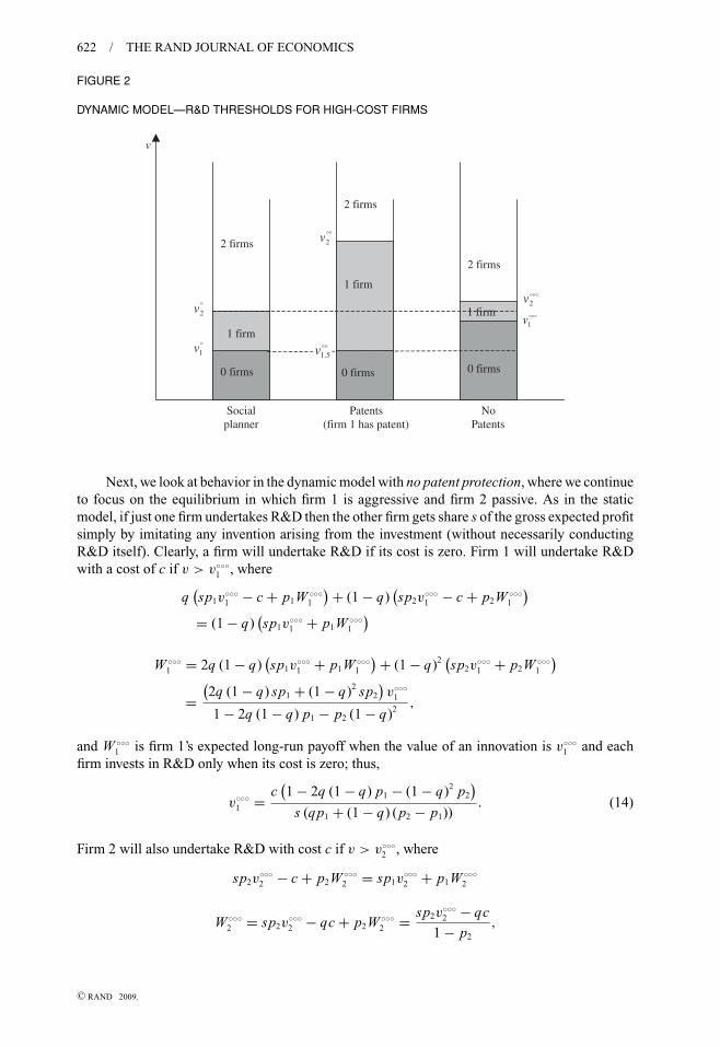
FIGURE 2

DYNAMIC MODEL—R&D THRESHOLDS FOR HIGH-COST FIRMS

1 firm

2 firms

1 firm

2 firms

0 firms

2 firms

Socialplanner

NoPatents

°1v

°2v

°°2v

°°°2v

v

1 firm°°°

1v

Patents(firm 1 has patent)

0 firms

°°5.1v

0 firms

Next, we look at behavior in the dynamic model with no patent protection, where we continueto focus on the equilibrium in which firm 1 is aggressive and firm 2 passive. As in the staticmodel, if just one firm undertakes R&D then the other firm gets share s of the gross expected profitsimply by imitating any invention arising from the investment (without necessarily conductingR&D itself). Clearly, a firm will undertake R&D if its cost is zero. Firm 1 will undertake R&Dwith a cost of c if v > v◦◦◦

1 , where

q(sp1v

◦◦◦1 − c + p1W ◦◦◦

1

) + (1 − q)(sp2v

◦◦◦1 − c + p2W ◦◦◦

1

)= (1 − q)

(sp1v

◦◦◦1 + p1W ◦◦◦

1

)W ◦◦◦

1 = 2q (1 − q)(sp1v

◦◦◦1 + p1W ◦◦◦

1

) + (1 − q)2(sp2v

◦◦◦1 + p2W ◦◦◦

1

)=

(2q (1 − q) sp1 + (1 − q)2 sp2

)v◦◦◦

1

1 − 2q (1 − q) p1 − p2 (1 − q)2 ,

and W ◦◦◦1 is firm 1’s expected long-run payoff when the value of an innovation is v◦◦◦

1 and eachfirm invests in R&D only when its cost is zero; thus,

v◦◦◦1 = c

(1 − 2q (1 − q) p1 − (1 − q)2 p2

)s (qp1 + (1 − q) (p2 − p1))

. (14)

Firm 2 will also undertake R&D with cost c if v > v◦◦◦2 , where

sp2v◦◦◦2 − c + p2W ◦◦◦

2 = sp1v◦◦◦2 + p1W ◦◦◦

2

W ◦◦◦2 = sp2v

◦◦◦2 − qc + p2W ◦◦◦

2 = sp2v◦◦◦2 − qc

1 − p2

,

C© RAND 2009.


and W ◦◦◦2 is firm 2’s expected long-run payoff when the value of each innovation is v◦◦◦

2 and bothfirms always invest in R&D32; thus,

v◦◦◦2 = c (1 − p2 + q (p2 − p1))

s (p2 − p1). (15)

From (12) and (14), we have v◦◦◦1 > v◦

1 . From (13) with (15) and because s < 12, we have

v◦◦◦2 > v◦

2 . Hence, we see that, as in the static model, there is too little R&D in equilibrium relativeto efficiency:

Proposition 5. In the sequential model, the equilibrium level of R&D investment in a regimewithout patents is less than or equal to the social optimum.

Although equilibrium without patents remains inefficient in the dynamic model, there isan important sense in which the inefficiency is smaller than that in the static model. To beginwith, notice, from (6) and (14), that v◦◦◦

1 < v∗∗∗1 and, from (9) and (15), that v◦◦◦

2 < v∗∗∗2 . That

is, the expected equilibrium levels of R&D in the dynamic model are higher than those in thestatic model (as we would anticipate since, in the sequential setting, investing in R&D raises theprobability not only of the next innovation but of subsequent innovation).

Still, the fact that there is more R&D in the dynamic model does not by itself settle the matterthat the dynamic equilibrium is more efficient. After all, efficiency also entails a higher expectedlevel of R&D in the sequential than the static model: from (2) and (12), v◦

1 < v∗1 , and, from (3)

and (13) v◦2 < v∗

2 . Nevertheless, under the same hypothesis invoked to show that patents are moreefficient than no patents in the static model (Proposition 2), we can show that equilibrium withoutpatents is more nearly efficient in the sequential than the static model:

Proposition 6. If the Upper Tail Condition holds for v̄ sufficiently big and k sufficiently small,then, for i = 1, 2, the likelihood that firm i behaves inefficiently in the sequential model withoutpatents is lower than that in the static model without patents.


To get a feel for why Proposition 6 holds, notice that the probability that firm 1’s behavioris inefficient in the static-model equilibrium without patents is the probability that v ∈ [v∗

1 , v∗∗∗1 ],

whereas the corresponding probability in the dynamic-model equilibrium without patents is theprobability that v ∈ [v◦

1, v◦◦◦1 ]. But the interval [v◦

1, v◦◦◦1 ] is smaller than [v∗

1 , v∗∗∗1 ], and the former

also lies below the latter. Hence if the density of F(v) does not drop off too rapidly as v increases,the probability that v ∈ [v◦

1, v◦◦◦1 ] is smaller than the probability that v ∈ [v∗

1 , v∗∗∗1 ]. The argument

is similar—although slightly more complicated—for firm 2.Equilibrium with patents is more complicated in the dynamic than the static model. To begin

with, when the model is dynamic, we must, distinguish between the R&D behavior of the twofirms before a patent is obtained on the first invention and their behavior after this patent isobtained (in the static model, by contrast, there is obviously no R&D after the patent is obtained).Furthermore, we have to consider the levels at which patent holders will set license fees, an issuethat also does not arise in the static model.

We suppose that a license gives a non-patent holder the possibility of developing the nextinnovation without infringing the patent. Moreover we assume that the license is written in sucha way that there is no dissipation of profit for the current innovation (because the license limitsthe total quantity sold). Finally, we suppose that the property rights to the next innovation accrueto the original patent holder (so that the licensing arrangement must award a non-patent holder

32 At v = v◦◦◦2 , firm 2 is indifferent between investing and not investing when its cost is c. Hence, we could

alternatively (and equivalently) have defined W ◦◦◦2 as 2’s expected long-run payoff when firm 1 always invests and firm 2

invests only if its cost is zero.

C© RAND 2009.


a sufficient share of the profit from that innovation if that firm is to be willing to incur the R&Dcost).

As we have done all along, we shall focus on the equilibrium in which firm 1 is aggressiveand firm 2 is passive.33 If inventions are protected by patents, each firm will invest if its cost iszero and neither firm yet has a patent. A firm will also invest if its cost is zero and it has a patent.If neither firm yet has a patent, firm 1 will invest if its cost is c and v > v◦◦

.5 , where

qp1

(v◦◦

.5 + W ◦◦.5

) + 1

2(1 − q) p2

(v◦◦

.5 + W ◦◦.5

) − c = 0 (16)

W ◦◦.5 = 2q(1 − q)p1

(v◦◦

.5 + W ◦◦.5

) + (1 − q)2 p2

(v◦◦

.5 + W ◦◦.5

)=

(2q(1 − q)p1 + (1 − q)2 p2

)v◦◦

.5

1 − 2q(1 − q)p1 − (1 − q)2 p2

,(17)

and W ◦◦.5 is the expected long-run payoff of a firm that holds a patent when the value of an

innovation is v◦◦.5 , if it conducts R&D only when its cost for the next innovation is zero and

licenses the other firm only when that firm’s cost is zero, that is, it sets the license fee so highthat only a low-cost firm will accept. More specifically, when only a low-cost firm is licensed,the patent holder gets the entire joint profit for itself.34 This outcome is reflected in formula (17):note that 2q(1 − q)p1v

◦◦.5 + (1 − q)2 p2v

◦◦.5 is the total expected surplus generated when each firm

does R&D if and only if its cost is zero. From (16) and (17), we have

v◦◦.5 =

(1 − 2q (1 − q) p1 − (1 − q)2 p2

)c

qp1 + 12

(1 − q) p2

. (18)

If neither firm yet has a patent, firm 2 will also invest in R&D when its cost is c, if v > v◦◦.75,

where

1

2p2

(v◦◦

.75 + W ◦◦.75

) − c = 0,

W ◦◦.75 =

(2q (1 − q) p1 + (1 − q)2 p2

)v◦◦

.75

1 − 2q (1 − q) p1 − (1 − q)2 p2

,

and W ◦◦.75 is the expected long-run payoff of a patent holder, when the value of an innovation is

v◦◦.75, if it conducts R&D only when its cost is zero and licenses the other firm only when that

firm’s cost is zero. Hence,

v◦◦.75 =

(1 − 2q (1 − q) p1 − (1 − q)2 p2

)c

12

p2

. (19)

A firm with a patent will invest in R&D with a cost of c (as opposed to just licensing) ifv > v◦◦

1.5, where

33 This asymmetry pertains only to the situation before one of the firm obtains a patent; after that point, the onlyasymmetry is between the patent holder and the other firm.

34 Implicit in this conclusion is the assumption that the patent holder has all the bargaining power in setting thelicense fee. That is, it can make a take-it-or-leave-it offer to the other firm. But if we assumed instead that the other firmshares in the bargaining power, none of our qualitative conclusions would change.

C© RAND 2009.


q p1

(v◦◦

1.5 + W ◦◦1.5

) + (1 − q)p2

(v◦◦

1.5 + W ◦◦1.5

) − c = (1 − q)p1

(v◦◦

1.5 + W ◦◦1.5

)W ◦◦

1.5 = q2(

p1

(v◦◦

1.5 + W ◦◦1.5

) − c) + q (1 − q)

(p2

(v◦◦

1.5 + W ◦◦1.5

) − c)

+ (1 − q) qp1

(v◦◦

1.5 + W ◦◦1.5

) + (1 − q)2 p2

(v◦◦

1.5 + W ◦◦1.5

)= (qp1 + (1 − q) p2) v◦◦

1.5 − qc

1 − qp1 − (1 − q) p2

,

and W ◦◦1.5 is the expected long-run payoff of a patent holder when the value of each innovation is

v◦◦1.5, if it invests when its cost is c and licenses the other firm only when that firm’s cost is zero.

Hence,

v◦◦1.5 =

(1 − 2q (1 − q) p1 − (1 − q)2 p2

)c

qp1 + (1 − q) (p2 − p1). (20)

Notice, from (19) and (20), that we have presumed that the v-threshold at which firm 2 withcost c does R&D when neither firm has a patent is less than that at which a firm with a patent doesR&D when its cost is c. However, it is readily verified that (19) is indeed less than (20) providedthat q is sufficiently small—and the latter is a hypothesis of the propositions we are coming to.

A firm with a patent will license the other firm (and perform R&D itself) even if that otherfirm’s cost is c provided that v > v◦◦

2 , where

p2

(v◦◦

2 + W ◦◦2

) − c = qp1

(v◦◦

2 + W ◦◦2

) + (1 − q)p2

(v◦◦

2 + W ◦◦2

), (21)

W ◦◦2 = p2

(v◦◦

2 + W ◦◦2

) − (1 + q) c = p2v◦◦2 − (1 + q) c

1 − p2

, (22)

and W ◦◦2 is the expected long-run payoff of a patent holder, when the value of each innovation

is v◦◦2 , if it always invests in R&D and always licenses the other firm. By licensing the other

firm even in the event that it has a high cost of R&D, the patent holder raises the probability ofdiscovery from p1 to p2 in that event, but must reduce its license fee by c (and, because costs areprivate information, it must do so even when the other firm’s cost is low35).36 From (21) and (22),we have

v◦◦2 =

(1 − (q + q2)p1 − (1 − q − q2)p2

)c

q (p2 − p1). (23)

Once again, we have presumed the ranking of threshold values: implicit in (20) and (23) is thepresumption that v◦◦

1.5 < v◦◦2 . That this is indeed the case is easily shown as long as q is sufficiently

small, which the following result assumes:

35 Thus, in this case, the other firm will earn a rent of c if its cost is low. Moreover, to ensure that the firm willactually undertake R&D when its cost is high, the patent holder must cede it some of the profit if the discovery is made(which the patent holder can take back in the form of a higher license fee).

36 We have been assuming that a firm wishing to build on a patented invention must first obtain a license from thepatent holder (see footnote 33). But let us imagine that the firm instead goes ahead and attempts to develop the nextinnovation without a license. If taking this next step entails first marketing some imitation of the patented item, then thefirm can expect to be sued for patent infringement and so presumably will not proceed in this way. But suppose that it canpotentially move to the next generation without direct market experience in the current generation. In that case, if it issuccessful, it can apply for a license ex post (see Scotchmer, 1996 and 2005, for treatments of ex post licensing). Notice,however, that the patent holder will then set a license fee that appropriates all of the firm’s profit from its invention.Furthermore, in contrast to ex ante licensing, the patent holder will not reduce this fee by c, even if that was the firm’sR&D cost, because this expenditure has already been sunk. Thus, a firm with R&D cost c will do worse by waiting forex post licensing (the analysis would be a bit more involved if the firm had some bargaining power in determining thelicense fee, but as footnote 34 points out, our qualitative conclusions would remain the same.)

C© RAND 2009.


Proposition 7. If the Upper Tail Condition holds for v̄ sufficiently big and k sufficiently small,then there exists q̄ > 0 such that expected net social welfare in the dynamic model is higherin equilibrium without patent protection than in equilibrium with such protection provided thatq < q̄ .


Remark. Note that this result holds even for small (but positive) values of s, that is, even withsubstantial dissipation of rents in the no-patent case. Moreover, one can show that it does notdepend on the assumption that the development cost for a low-cost type is zero; it holds fora positive lower cost as well. Finally, notice that we have considered private information onlyregarding development costs. But because rivals are presumably using different technologies,private information about production costs is also likely. This would lead to a broader range ofcircumstances in which patents would generate lower social welfare.

To get a feel for why Proposition 7 holds, let us suppose that higher values of v are muchmore likely than lower values (which is considerably stronger than the actual hypothesis). If thereis no patent protection, then, as derived in (15), firm 2 will undertake R&D with cost c as long as

(◦) v >c (1 − p2 + q (p2 − p1))

s (p2 − p1)

(= v◦◦◦2

).

In a regime with patent protection, by contrast, once one firm has a patent, it will refrainfrom setting the license fee low enough so that the other firm will undertake R&D with cost c,if the patent holder’s expected benefit from the additional R&D, q(p2 − p1)(v + W ), is less thanthe loss in fee revenue c from setting the lower fee, that is, if

(◦◦) v <

(1 − (

q + q2)

p1 − (1 − q − q2

)p2

)c

q (p2 − p1)

(= v◦◦2

).

But if q is small, then the right-hand side of (◦◦)exceeds the right-hand side of (◦). Thus, forv ∈ [v◦◦◦

2 , v◦◦2 ], society gets more R&D investment when there is no patent protection than when

such protection is available.37 And since there is underinvestment anyway in the absence of patentprotection, this additional R&D is socially beneficial, that is, for this interval, “no patents” arebetter than “patents.” Now, of course, for lower values of v, the comparison can go the other way.But if higher values are sufficiently more likely than lower values, we can conclude that havingno patent protection is better on average.38

This conclusion remains even if we take into account the overall effect of patents on R&D.Indeed, suppose we focus purely on the incentives of firms to undertake R&D before a patenthas been obtained. Then, we see from (12) and (18), that v◦◦

.5 < v◦1 and, from (13) and (19) that

v◦◦.75 < v◦

2 if q is sufficiently small. That is, firms will tend to overinvest, as in the static model(see Proposition 1). But this overinvestment result pertains only to the first innovation, whereasthe underinvestment logic applies to all subsequent innovations. Hence, under the very conditionthat makes the case for patents compelling in the static model, overinvestment is more thancounterbalanced in the dynamic model by the constraint on R&D imposed by the patent holder’sunwillingness to license a high-cost firm.

If s ≈ 12—so that there is little profit dissipation—then most of the net social welfare

generated without patents accrues to the firms themselves. Hence, in that case, we can concludethat ex ante the firms themselves will prefer that innovations not be protected by patents:

37 If, by contrast, q is near 1, then the patent holder will set a relatively low license fee, and, in fact, licensing willoccur at nearly the socially efficient rate. Thus, in this case, patents will dominate the absence of patent protection froma social standpoint.

38 Boldrin and Levine (2004) show that the inefficiencies of patents are aggravated if a firm has to obtain licensesfrom different patent holders in order to innovate.

C© RAND 2009.


Proposition 8. If the Upper Tail Condition holds for v̄ sufficiently big and k sufficiently small,then each firm’s ex ante expected profit in the dynamic model is higher in equilibrium withoutpatent protection than in equilibrium with protection, provided that q is sufficiently small and s isnear enough 1

2.


Remark. The conclusion of Proposition 8 depends critically on neither firm having a patent exante. It is evident that once a firm obtains such protection, it will definitely prefer to keep it andexercise monopoly power in licensing, even though this may reduce innovation and thereforetotal profit. But this observation prompts the question why, before any discovery has beenmade, the firms do not enter an agreement to ensure that licensing always occurs regardlessof which of them ends up getting the patent on the first discovery. Such an arrangement wouldbe desirable both for the firms and society. It would, however, require the two firms to knowof one another’s existence before the industry has even begun, which could be a very tall orderindeed.

Finally, we turn to a fourth important difference between the static and sequential models:whether or not an innovating firm itself benefits from competition and being imitated. InProposition 3, we showed that a firm undertaking R&D clearly loses from competition andimitation in the static model. By contrast, in the sequential model we have:

Proposition 9. Assume that the Upper Tail Condition holds for v̄ sufficiently big and k sufficientlysmall and that

p2 >2p1

1 + p1

. (24)

If s is near enough 12, then in the sequential model a firm gains from having a competitor and

being imitated, whether or not there is patent protection.


Remark 1. Proposition 9 is a formal justification for the dictum that “competition expands themarket” and explains Apple’s welcoming greeting to IBM (see footnote 4).

Remark 2. Condition (24) holds if, for example, p1 = p and p2 = 1 − (1 − p)2, that is, if thetwo firms’ chances of success are statistically independent.

Remark 3. Propositions 6–9 suggest another reason beyond empirical realism for invoking theUpper Tail Condition.39 As we noted in Section 2, the welfare comparison between the patentand no-patent regimes is ambiguous in the absence of any assumption about the distribution ofreturns: the absence of patents leads to underinvestment in R&D, but, in the static model, patentsinduce overinvestment. Because something like the Upper Tail Condition is needed to generatethe standard conclusion that, on balance, patents are desirable in a static setting, it is of interestto see that this same condition invoked in a sequential setting leads to quite different results:the no-patent regime is now closer to efficiency than in the static model; patents may generateless innovation than in the absence of patents; and imitation may be welcomed by inventorsthemselves.

Having a competitor may be advantageous to a would-be inventor because, for v big enough(which, given the Upper Tail Condition, is sufficiently likely), this other firm will undertake R&Dtoo and thereby raise the probability of discovery from p1 to p2, which improves the inventor’s

39 We have established these propositions under the hypothesis that new inventions enhance rather than replace oldinventions, but the qualitative contrast between the static and dynamic models—on which Proposition 6 turns—and theunwillingness of a patent holder to license high-cost competitors—on which Propositions 7–9 turn—do not depend onthis distinction. Hence, the propositions can be shown to hold for replacement.

C© RAND 2009.


future profit. Of course, there is also the drawback that the competitor obtains a share of thisprofit. But if s is not too small, this latter effect is outweighed by the former.

4. Conclusion

� Intellectual property appears to be an area in which results that seem secure in a static modelmay be overturned in a sequential setting. The prospect of being imitated inhibits inventors in astatic world; in a dynamic world, imitators can provide benefit to both the original inventor andto society more generally. Patents may be desirable to encourage innovation in a static world, butthey are less important in a sequential setting, where they may actually inhibit complementaryinnovation.

The static-sequential distinction is more than just a theoretical nicety. Indeed, it may helpresolve a puzzle emanating from the U.S. natural experiment in software patents. Strikingly,the firms that obtained the most software patents (largely firms in the computer and electronicshardware industries) actually reduced their R&D spending relative to sales after patent protectionwas strengthened (Bessen and Hunt, 2004). This behavior is difficult to reconcile with the staticmodel, in which the prospect of patents should encourage R&D, but is quite consistent with thesequential model and specifically Proposition 7.

Thus we would suggest a cautionary note about intellectual property protection. The reflexiveview that “stronger is better” could well be too extreme; rather, a balanced approach seems calledfor. The ideal patent policy limits “knockoff” imitation, but allows developers who make similar,but potentially valuable complementary contributions. In this sense, copyright protection forsoftware programs (which has gone through its own evolution over the last decade) may haveachieved a better balance than patent protection. In particular, industry participants complain thatsoftware patents have been too broad (and patented discoveries too obvious), leading to holdupproblems (USPTO 1994, Oz 1998). Systems that limit patent breadth, such as in the Japanesesystem before the late 1980s, may offer a better balance.40

Appendix A

� Proof that the Pareto distribution satisfies the Upper Tail Condition. The Pareto distribution is

F(v) = 1 −(

v0

v

)α

, v0 ≤ v, 0 < α,

so that

d2 F(v)

dv2= −α(1 + α)

vα0

v2+α.

Since limα→0d2 F(v)

dv2 = 0 ≥ −k, we see that, given k and v̄, the Pareto distribution satisfies the Upper Tail Conditionfor k and v̄ for all v in the defined domain, provided that α is small enough and v0 = c

p1.

� Proof that the lognormal distribution satisfies the Upper Tail Condition for values of v above the median. Forthe lognormal distribution with parameters μ and σ ,

d F

dv(v) = Exp[− (ln(v) − μ)2

/2σ 2]

σv√

2π

and the median value of v is eμ. Thus,

d2 F(v)

dv2= − Exp[(ln(v) − μ)2/2σ 2]

(ln(v) − μ + σ 2

)σ 3v2

√2π

.

40 In a review of the literature, Gallini and Scotchmer (2001) conclude, “Thus, with some caution, we can extractfrom the literature a case for broad (and short) patents. Broad patents can serve the public interest by preventing duplicationof R&D costs, facilitating the development of second generation products, and protecting early innovators who lay afoundation for later innovators. However, these benefits disappear if licensing fails.” Our model establishes that broadpatents may be especially harmful if licensing fails and that there is good reason to expect such a failure.

C© RAND 2009.


It is then straightforward to show that

d2 F(v)

dv2

∣∣∣∣v=eμ

= − e−2μ

σ√

2π≤ d2 F(v)

dv2, ∀v ∈ [eμ, ∞] .

Since, for any k > 0, limσ→∞ .d2 F(v)

dv2 |v=eμ = 0 ≥ −k, the lognormal distribution satisfies the Upper Tail Condition for allv above the median, given a large enough value of σ .

Appendix B

� Proofs of the Propositions

Proposition 2. If the Upper Tail Condition holds for v̄ sufficiently big and k sufficiently small, then expected net socialwelfare in the static model is higher with patent protection than without it.

Proof . The expected difference in welfare between having patents and not having patents as this relates to firm 1’sparticipation is:∫ v∗

1

v∗∗1

[q (1 − q) ((p2 − p1) v − c) + q2 (p1v − c)

]d F(v) +

∫ v∗∗∗1

v∗1

[q (1 − q) ((p2 − p1) v − c) + q2 (p1v − c)

]d F(v),

(B1)

where the first integral in (B1) is negative because of overinvestment under patent protection (the fact that v∗∗1 < v∗

1 ) andthe second integral is positive because of underinvestment without patent protection (the fact that v∗

1 < v∗∗∗1 ). Summing

the two integrals, we must show that for k small enough and v̄ big enough,∫ v∗∗∗1

v∗∗1

[av − c] d F(v) (B2)

is positive, where a = qp1 + (1 − q)(p2 − p1). We can rewrite (B2) as

(F

(v∗∗∗

1

) − F(v∗∗

1

)) ∫ v∗∗∗1

v∗∗1

(av − c) d F1 (v) (B3)

where F1(v) = F(v)−F(v∗∗1 )

F(v∗∗∗1 )−F(v∗∗

1 ) , so that

F1

(v∗∗

1

) = 0 and F1

(v∗∗∗

1

) = 1. (B4)

To show that (B2) is positive, it suffices, from (B3), to show that∫ v∗∗∗1

v∗∗1

(av − c) d F1 (v) > 0 (B5)

After integration by parts, the left-hand side of (B4) can be written as

av∗∗∗1 − c − a

∫ v∗∗∗1

v∗∗1

F1 (v) dv. (B6)

From the hypothesis of Proposition 2, we can choose k sufficiently small and v̄ sufficiently big that

F1 (v) ≤(

v

v∗∗∗1 − v∗∗

1

− v∗∗1

v∗∗∗1 − v∗∗

1

)+ v∗∗

1

2 (v∗∗∗1 − v∗∗

1 )for all v ∈ [

v∗∗1 , v∗∗∗

1

](B7)

From (B7), (B6) exceeds

av∗∗∗1 − c − 1

v∗∗∗1 − v∗∗

1

[a

2

((v∗∗∗

1

)2

− (v∗∗

1

)2)]

+ av∗∗1

2= av∗∗∗

1

2− c,

which is positive because a2v∗∗∗

1 − c = c2s

− c > 0.The expected difference in welfare between having patents and not having patents as this relates to firm 2’s

participation is

q

∫ v∗2

v∗∗2

((p2 − p1) v − c) d F (v) + q

∫ v∗∗∗2

v∗2

((p2 − p1) v − c) d F (v), (B8)

where the first integral in (B8) is negative because of overinvestment by firm 2 with patents (the fact that v∗∗2 < v∗

2 ) andthe second is positive because of underinvestment by firm 2 without patents (the fact that v∗

2 < v∗∗∗2 ). Summing the two

integrals and dividing by q, we must show that∫ v∗∗∗2

v∗∗2

((p2 − p1) v − c) d F (v) (B9)

C© RAND 2009.


is positive for k sufficiently small and v̄ sufficiently big. We can rewrite (B9) as

(F

(v∗∗∗

2

) − F(v∗∗

2

)) ∫ v∗∗∗2

v∗∗2

((p2 − p1) v − c) d F2 (v) (B10)

where F2(v) = F(v)−F(v∗∗2 )

F(v∗∗∗2 )−F(v∗∗

2 ) , so that

F2

(v∗∗

2

) = 0 and F2

(v∗∗∗

2

) = 1. (B11)

To show that (B9) is positive, it suffices, from (B10), to show that∫ v∗∗∗2

v∗∗2

((p2 − p1) v − c) d F2 (v) > 0. (B12)

After integration by parts, the left-hand side of (B12) can be written as

(p2 − p1) v∗∗∗2 − c − (p2 − p1)

∫ v∗∗∗2

v∗∗2

F2 (v) dv. (B13)

From hypothesis, we can choose k sufficiently small and v̄ sufficiently big so that

F2 (v) ≤(

v

v∗∗∗2 − v∗∗

2

− v∗∗2

v∗∗∗2 − v∗∗

2

)+ v∗∗

2

2(v∗∗

2 − v∗∗∗2

) (B14)

From (B14), (B13) exceeds

(p2 − p1) v∗∗∗2 − c − (p2 − p1)

⎛⎝(

v∗∗∗2

)2 − (v∗∗

2

)2

2(v∗∗∗

2 − v∗∗2

) − v∗∗2

2

⎞⎠

= (p2 − p1) v∗∗∗2

2− c

= c

2s− c,

which is positive because c2s

− c > 0. Q.E.D.

Proposition 3. In the static model, a firm undertaking R&D is (weakly) worse off if it has a competitor.

Proof . When the firm has no competitor, its expected payoff is, depending on its cost,

p1v or p1v − c, (B15)

If there is no patent protection and the firm faces a competitor, its payoff is

sp1v or sp1v − c when the other firm simply imitates

or

sp2v or sp2v − c when the other firm also invests,

all of which are less than their counterparts in (B15). If instead there is patent protection, then the firm’s payoff is (B15)when the other firm does not invest and

1

2p2v or

1

2p2v − c when the other firm invests, (B16)

which is each less than its counterpart in (B15). Q.E.D.

Proposition 4. In the static model, a firm undertaking R&D is better off if there is patent protection than if there is nosuch protection.

Proof . If there is patent protection, then a firm that undertakes R&D with cost c has payoff either(qp1 + 1

2(1 − q) p2

)v − c or

1

2p2v − c,

depending on whether or not the other firm does too. If instead there is no protection, the payoffs are

(sqp1 + s (1 − q) p2) v − c or sp2v − c.

C© RAND 2009.


But

(sqp1 + s (1 − q) p2) v < sp2v <1

2p2v <

(qp1 + 1

2(1 − q) p2

)v,

and so the firm is better off with patent protection. Q.E.D.

Proposition 6. If the Upper Tail Condition holds for v̄ sufficiently big and k sufficiently small, then, for i = 1, 2, thelikelihood that firm i behaves inefficiently in the sequential model without patents is lower than that in the static modelwithout patents.

Proof . For i = 1, 2 the probability of inefficiency for firm i without patent protection in the static model is

F(v∗∗∗

i

) − F(v∗

i

), (B17)

whereas that in the dynamic model is

F(v◦◦◦

i

) − F(v◦

i

). (B18)

Now, from (2), (6), (12) and (14),(v∗

1 , v∗∗∗1

)= 1

1 − 2q(1 − q)p1 − (1 − q)2 p2

(v◦

1 , v◦◦◦1

)(B19)

If v̄ is sufficiently big and k sufficiently small, the Upper Tail Condition implies that F(xv◦◦◦1 ) − F(xv◦

1 ) is increasing inx, for x ∈ [1, 1

1−2q(1−q)p1−(1−q)2 p2]. Hence, we conclude from (B19) that

F(v∗∗∗

1

) − F(v∗

1

)> F

(v◦◦◦

1

) − F(v◦

1

). (B20)

Similarly, we have

(v∗

2 , v∗∗∗2

) = 1

1 − p2 + 2q (p2 − p1)

(v◦

2 ,c (1 − p2 + 2q(p2 − p1))

s(p2 − p1)

),

And so, from the Upper Tail Condition, we obtain

F(v∗∗∗

2

) − F(v∗

2

)> F

(c (1 − p2 + 2q(p2 − p1))

s(p2 − p1)

)− F

(v◦

2

)> F

(v◦◦◦

2

) − F(v◦

2

). (B21)

Hence from (B20) and (B21), (B17) is bigger than (B18). Q.E.D.

Proposition 7. If the Upper Tail Condition holds for v̄ sufficiently big and k sufficiently small, then there exists q̄ > 0such that, expected net social welfare in the dynamic model is higher in equilibrium without patent protection than inequilibrium with such protection provided that q < q̄.

Proof . For q near enough 0, we have, from (12)–(15), (18)–(20), and (23)

v◦◦.5 < v◦◦

.75 < v◦◦1.5 = v◦

1 < v◦2 < v◦◦◦

1 < v◦◦◦2 < v◦◦

2 .

Hence, the expected difference in welfare between having patents and not having them is∫ v◦◦.75

v◦◦.5

[(qp1 + (1 − q) p2) v

1 − 2q (1 − q) p1 − (1 − q)2 p2

− qc −(2q (1 − q) p1 + (1 − q)2 p2

)v

1 − 2q (1 − q) p1 − (1 − q)2 p2

]dF (v)

+∫ v◦◦

1.5

v◦◦.75

[p2v

1 − 2q (1 − q) p1 − (1 − q)2 p2

− 2qc −(2q (1 − q) p1 + (1 − q)2 p2

)v

1 − 2q (1 − q) p1 − (1 − q)2 p2

]dF (v)

+∫ v◦◦◦

1

v◦◦1.5

[p2 (v − qc)

1 − qp1 − (1 − q) p2

− 2qc −(2q (1 − q) p1 + (1 − q)2 p2

)v

1 − 2q (1 − q) p1 − (1 − q)2 p2

]dF (v)

+∫ v◦◦◦

2

v◦◦◦1

[p2 (v − qc)

1 − qp1 − (1 − q) p2

− 2qc − (qp1 + (1 − q) p2) v − qc

1 − qp1 − (1 − q) p2

]dF (v)

+∫ v◦◦

2

v◦◦◦2

[p2 (v − qc)

1 − qp1 − (1 − q) p2

− 2qc − p2v − 2qc

1 − p2

]dF (v). (B22)

It will suffice to show that there exists A > 0 such that, for q sufficiently near 0, (B22) is less than −A.As q → 0, the integrands of the first four integrals of (B22) tend to zero. Furthermore, v◦◦

.5 , v◦◦.75, v◦◦

1.5, v◦◦◦1 , and v◦◦◦

2

all tend to finite limits. Hence, the first four integrals all tend to zero as q → 0. To understand the fifth integrand, notethat the social payoff from having patents is

p2v − 2qc + p2W ◦◦1.5 = p2 (v − qc)

1 − qp1 − (1 − q) p2

− 2qc,

C© RAND 2009.


whereas the social payoff when there is no patent protection is

p2v − 2qc

1 − p2

.

Now, the fifth integral can be written as

(F

(v◦◦

2

) − F(v◦◦◦

2

)) ∫ v◦◦2

v◦◦◦2

(a◦v + b) dF∗ (v) + F(v◦◦◦

2

) ∫ v◦◦2

v◦◦◦2

(a◦v + b) dv,

where

F∗ (v) = F (v) − F(v◦◦◦

2

)F (v◦◦

2 )

a◦ = qp2 (p1 − p2)

(1 − qp1 − (1 − q) p2) (1 − p2)

and

b = q(

p2 − p22 − 2qp1 p2 + 2qp2

2

)c

(1 − qp1 − (1 − q) p2) (1 − p2).

Hence, it suffices to show that there exist D > 0 and E > 0 such that∫ v◦◦2

v◦◦◦2

(a◦v + b) dv < −D (B23)

∫ v◦◦2

v◦◦◦2

(a◦v + b) dF∗ (v) < −E (B24)

for q near enough 0. The left-hand side of (B23) can be rewritten as

a◦

2

[(v◦◦

2

)2 − (v◦◦◦

2

)2]

+ b(v◦◦

2 − v◦◦◦2

). (B25)

Because

v◦◦2 ≈ (1 − p2) c

q (p2 − p1), a◦ ≈ qp2 (p1 − p2)

(1 − p2)2

b ≈ q(

p2 − p22

)c

(1 − p2)2 for q ≈ 0, (B26)

the limit of (B25) as q → 0 is −∞, and so (B23) holds. The left-hand side of (B24) can be rewritten as

a◦v◦◦2 + b − a◦

∫ v◦◦2

v◦◦◦2

F∗ (v) dv. (B27)

For k small enough and v̄ big enough, the Upper Tail Condition ensures that

F∗ (v) ≤(

v

v◦◦2 − v◦◦◦

2

− v◦◦◦2

v◦◦2 − v◦◦◦

2

)+ v◦◦◦

2

2 (v◦◦2 − v◦◦◦

2 ). (B28)

From (B28), (B27) is no greater than

a◦v◦◦2 + b − a

2

(v◦◦

2 + v◦◦◦2

) + a◦v◦◦◦2

2= a◦

2v◦◦

2 + b, (B29)

and from (B26), the limit of the right-hand side of (B29) as q → 0 is

−p2c

2 (1 − p2),

and so (B24) holds. Q.E.D.

Proposition 8. If the Upper Tail Condition holds for v̄ sufficiently big and k sufficiently small, than each firm’s exante expected profit in the dynamic model is higher in equilibrium without patent protection than in equilibrium withprotection, provided that q is sufficiently small and s is near enough 1

2.

C© RAND 2009.


Proof . Following the argument in the proof of Proposition 7, we can express the difference in firm 1’s payoff betweenequilibrium with and without patents, assuming q is sufficiently small, as∫ v◦◦

1.5

v◦◦.5

[ (qp1 + (1 − q) 1

2p2

)v

1 − 2q (1 − q) p1 − (1 − q)2 p2

− qc − s(2q (1 − q) p1 + (1 − q)2 p2

)v

1 − 2q (1 − q) p1 − (1 − q)2 p2

]dF (v)

+∫ v◦◦

1.5

v◦◦.5

[12

p2

1 − 2q (1 − q) p1 − (1 − q)2 p2

− qc − s(2q (1 − q) p1 + (1 − q)2 p2

)v

1 − 2q (1 − q) p1 − (1 − q)2 p2

]dF (v)

+∫ v◦◦◦

1

v◦◦.5

[12

p2 (v − qc)

1 − qp1 − (1 − q) p2

− qc − s(2q (1 − q) p1 + (1 − q)2 p2

)v

1 − 2q (1 − q) p1 − (1 − q)2 p2

]dF (v)

+∫ v◦◦◦

2

v◦◦◦1

[12

p2 (v − qc)

1 − qp1 − (1 − q) p2

− qc − s (qp1 + (1 − q) p2) v − qc

1 − qp1 − (1 − q) p2

]dF (v)

+∫ v◦◦

2

v◦◦◦2

[12

p2 (v − qc)

1 − qp1 − (1 − q) p2

− qc − sp2v − qc

1 − p2

]dF (v) .

(B30)

As q → 0, the integrands of the first four integrals of (B30) tend to zero and v◦◦.5 , v◦◦

.75, v◦◦1.5, v◦◦◦

1 , and v◦◦◦2 tend to

finite limits, as in the proof of Proposition 7. Hence, as in that proof, the first four integrals all tend to zero as q → 0.Furthermore, for s near 1

2, the fifth integral is about half that of its counterpart in (B22). Hence, by the same logic as in

the previous proof, (B30) is negative, given the hypotheses. Q.E.D.

Proposition 9. Assume that the Upper Tail Condition holds for v̄ sufficiently big and k sufficiently small and that

p2 >2p1

1 + p1

. (24)

If s is near enough 12, then in the sequential model a firm gains from having a competitor and being imitated, whether or

not there is patent protection.

Proof . If a firm has no competitor, its payoff for v big enough is

p1v − qc

1 − p1

. (B31)

By contrast in two-firm equilibria with and without patents, a firm’s payoffs, for v big enough, are, respectively,12

(p2v − 2qc)

1 − p2

(B32)

andsp2v − qc

1 − p2

. (B33)

Now, because (24) holds, sp2

1−p2> p1v

1−p2for s near 1

2. Hence, for v big enough, (B32) and (B33) are bigger than (B31).

We conclude that for k small enough and v̄ big enough, a firm’s equilibrium payoff with competition is bigger than thatwithout competition. Q.E.D.

References

AHARONIAN, G. Patent News Service, 1995.BESSEN, J. “Patents and the Diffusion of Technical Information.” Economics Letters, Vol. 86, (2005), pp. 121–

128.—— AND HUNT, R. “An Empirical Look at Software Patents.” Federal Reserve Bank of Philadelphia Working Paper no.

03-17, 2004.—— AND MEURER, M. Patent Failure: How Judges, Bureaucrats and Lawyers Put Innovators at Risk. Princeton, N.J.:

Princeton University Press, 2008.BOLDRIN, M. AND LEVINE, D. “The Economics of Ideas and Intellectual Property.” Proceedings of the National Academy

of Sciences, Vol. 102 (2004), pp. 1252–1256.CHANG, H. “Patent Scope, Antitrust Policy and Cumulative Innovation.” RAND Journal of Economics, Vol. 26 (1995),

p. 34.DASGUPTA, P. AND MASKIN, E. “The Simple Economics of Research Portfolios.” The Economic Journal, Vol. 97 (1987),

p. 581.

C© RAND 2009.


—— AND STIGLITZ, J. “Uncertainty, Industrial Structure, and the Speed of R&D.” Bell Journal of Economics, Vol. 11(1980), p. 1.

FERSHTMAN, C. AND KAMIEN, M. “Cross Licensing of Complementary Technologies.” International Journal of IndustrialOrganization, Vol. 10 (1992), p. 329.

GALLINI, N. “Deterrence through Market Sharing: A Strategic Incentive for Licensing.” American Economic Review,Vol. 74 (1984), pp. 931–941.

—— AND SCOTCHMER, S. “Intellectual Property: When Is It the Best Incentive System?” In A. Jaffe, J. Lerner and S.Stern, eds., Innovation Policy and the Economy, Volume 2. Cambridge, Mass.: MIT Press, 2001.

—— AND WINTER, R. “Licensing in the Theory of Innovation.” RAND Journal of Economics, Vol. 16 (1985), pp. 237–252.GREEN, J. AND SCOTCHMER, S. “On the Division of Profit in Sequential Innovation.” RAND Journal of Economics, Vol. 26

(1995), p. 20.GROSSMAN, S. “A Characterization of the Optimality of Equilibrium in Incomplete Markets.” Journal of Economic Theory,

Vol. 15 (1977), pp. 1–15.HUNT, R. “Patentability, Industry Structure, and Innovation.” Journal of Industrial Economics, Vol. 52 (2004),

pp. 401–425.KATZ, M. AND SHAPIRO, C. “On the Licensing of Innovation.” RAND Journal of Economics, Vol. 16 (1985), pp. 504–520.—— AND ——. “How To License Intangible Property.” Quarterly Journal of Economics, Vol. 101 (1986), pp. 567–589.KEELY, L. 2005. “Choosing to Exchange Research Ideas.” Unpublished.LEMLEY, M. “The Economics of Improvement in Intellectual Property Law.” Texas Law Review, Vol. 75 (1997),

pp. 989–1084.LEVIN, R., KLEVORICK, A., NELSON, R., AND WINTER, S. “Appropriating the Returns from Industrial Research and

Development.” Brookings Papers on Economic Activity, Vol. 3 (1987), p. 783.LOURY, G. “Market Structure and Innovation.” Quarterly Journal of Economic, Vol. 93 (1979), p. 395.MACHLUP, F. AND PENROSE, E. “The Patent Controversy in the Nineteenth Century.” The Journal of Economic History,

Vol. 10 (1950), pp. 1–29.MANSFIELD, E., SCHWARTZ, M., AND WAGNER, S. “Imitation Costs and Patents: An Empirical Study.” Economic Journal,

Vol. 91 (1981), p. 907.MOWERY, D. “Introduction.” In D. Mowery, ed., The International Computer Software Industry: A Comparative Study of

Industry Evolution and Structure. Oxford: Oxford University Press, 1996.O’DONOGHUE, T. “A Patentability Requirement for Sequential Innovation.” RAND Journal of Economics, Vol. 29 (1998),

pp. 654–679.——, SCOTCHMER, S., AND THISSE, J. “Patent Breadth, Patent Life and the Pace of Technological Progress.” Journal of

Economics and Management Strategy, Vol. 7 (1998), pp. 1–32.OZ, E. “Acceptable Protection of Software Intellectual Property: A Survey of Software Developers and Lawyers.”

Information & Management, Vol. 34 (1998), pp. 161–173.PAKES, A., AND SCHANKERMAN, M. “The Rate of Obsolescence of Patents, Research Gestation Lags, and the Private Rate

of Return to Research Resources.” In Z. Griliches, ed., R&D, Patents and Productivity. Cambridge, Mass.: NBER,1984.

SAKAKIBARA, M. AND BRANSTETTER, L. “Do Stronger Patents Induce More Innovation? Evidence from the 1998 JapanesePatent Law Reforms.” Rand Journal of Economics, Vol. 32 (2001), pp. 77–100.

SANDERS, B., ROSSMAN, J., AND HARRIS, L. “The Economic Impact of Patents.” Patent, Trademark and Copyright Journalof Research and Education, Vol. 2 (1958), p. 355.

SCHERER, F. AND HARHOFF, D. “Technology Policy for a World of Skew-Distributed Outcomes.” Research Policy, Vol. 29(2000), pp. 559–566.

SCOTCHMER, S. “Standing on the Shoulders of Giants: Cumulative Research and the Patent Law.” Journal of EconomicPerspectives, Vol. 5 (1991), pp. 29–41.

——. “Protecting Early Innovators: Should Second-Generation Products be Patentable?” RAND Journal of Economics,Vol. 27 (1996), p. 322.

——. Innovation and Incentives. Cambridge, Mass.: MIT Press, 2005.—— AND GREEN, J. “Novelty and Disclosure in Patent Law.” RAND Journal of Economics, Vol. 21 (1990), pp. 131–146.SHAVELL, S. AND YPERSELE, T. “Rewards vs. Intellectual Property Rights.” Journal of Law and Economics, Vol. 44 (2001),

pp. 525–548.SILVERBERG, G. AND VERSPAGEN, B. “The Size Distribution of Innovations Revisited: An Application of Extreme Value

Statistics to Citation and Value Measures of Patent Significance.” MERIT-Infonomics Research Memorandum no.2004-021, 2004.

SPENCE, M. “Cost Reduction, Competition, and Industry Performance.” Econometrica, Vol. 52 (1984), p. 101.SUTTON, J. Technology and Market Structure. Cambridge, Mass.: MIT Press, 1998.TANDON, P. “Rivalry and the Excessive Allocation of Resources to Research.” Bell Journal of Economics, Vol. 14 (1983),

pp. 152–165.TAYLOR, C. T. AND SILBERSTON, Z. A. The Economic Impact of the Patent System: A Study of the British Experience.

Cambridge, UK: Cambridge University, p. 294, 1973.

C© RAND 2009.


TILTON, J. International Diffusion of Technology: The Case of Semiconductors. Washington, D.C.: Brookings Institution,1971.

USPTO. “Hearings on Software Patent Protection.” United States Patent and Trademark Office, January–February 1994.WIGGINS, S. AND LIBECAP, G. “Oil Field Unitization: Contractual Failure in the Presence of Imperfect Information.”

American Economic Review, Vol. 75 (1985), pp. 368–385.WRIGHT, B. “The Economics of Invention Incentives: Patents, Prizes, and Research Contracts.” American Economic

Review, Vol. 73 (1983), pp. 691–707.

C© RAND 2009.

sequential innovation, patents, and imitation - home |...

Documents