separación de fuentes de descargas parciales y ruido ... · 3.4.2.3 identificación de pds en gis...

UNIVERSIDAD CARLOS III DE MADRID Escuela Politécnica Superior

Departamento de Ingeniería Eléctrica

TESIS DOCTORAL

“Separación de fuentes de descargas parciales y ruido eléctrico mediante análisis de potencia

espectral en alta frecuencia”

Autor: Jorge Alfredo Ardila Rey

Director: Dr. D. Juan Manuel Martínez Tarifa

Leganés (Madrid), Mayo 2014

III

TESIS DOCTORAL

“Separación de fuentes de descargas parciales y ruido eléctrico mediante análisis de potencia

espectral en alta frecuencia”

Autor: Jorge Alfredo Ardila Rey

Director: Dr. D. Juan Manuel Martínez Tarifa

Firma del Tribunal Calificador

Firma

Presidente: (Nombre y apellidos) Vocal: (Nombre y apellidos) Secretario: (Nombre y apellidos) Calificación:

Leganés, de de

V

“De rodillas ante Dios, para estar de pie ante los hombres.”

NÉSTOR CHAMORRO PESANTES.

“No fracasé, sólo descubrí 10.000 maneras de cómo no hacer una bombilla.”

THOMAS ALVA EDISON.

VII

Contenido

Contenido VII Lista de figuras XI Lista de tablas XVII Agradecimientos XIX Resumen XXI Abstract XXIII 1. Introducción

1.1. Motivación de la Tesis .................................................................................... 1 1.2. Finalidad y objetivos de la Tesis ..................................................................... 4 1.3. Estructura de la Tesis ...................................................................................... 5 Bibliografia ............................................................................................................ 6

2. Estado del arte

2.1. Introducción a las descargas parciales: descripción y fundamentos físicos ... 7 2.2. Tipos de descargas parciales ......................................................................... 11

2.2.1. PDs Internas. ......................................................................................... 11 2.2.2. PDs Superficiales.. ................................................................................ 14 2.2.3. PDs Corona ........................................................................................... 15 2.2.4. Identificación avanzada de fuentes de descargas parciales en

equipamiento eléctrico. ................................................................................... 16 2.3. Medición de descargas parciales ................................................................... 16

2.3.1. Técnicas ópticas .................................................................................... 17 2.3.2. Técnicas de emisión acústica ................................................................ 17 2.3.3. Técnicas químicas. DGA (“Disolved Gas Analysis”) ........................... 18 2.3.4. Técnicas RF (Radio Frequency) ............................................................ 18 2.3.5. Técnicas eléctricas ................................................................................ 19 2.3.6. Sensores inductivos para la detección de PDs ...................................... 20 2.3.6.1 HFCT ................................................................................................. 23 2.3.6.2 RC ...................................................................................................... 23 2.3.6.3 ILS ..................................................................................................... 23

2.4. Caracterización estadística de las PDs .......................................................... 24 2.4.1. Análisis estadístico de distribuciones de fase. ...................................... 25 2.4.2. Tratamiento estadístico de amplitudes y tasa de repetición de descargas

parciales. .......................................................................................................... 25 2.4.3. Identificación automática de patrones PRPD. ....................................... 27 2.4.3.1 Identificación de fuentes de PDs con algoritmos basados en lógica

fuzzy (lógica difusa) ..................................................................................... 27 2.4.3.2 Identificación de fuentes de PDs con redes neuronales:. .................. 28

Bibliografia .......................................................................................................... 28 3. Métodos de separación e identificación de fuentes de PDs y ruido en sistemas de detección

3.1. Separación de PDs y ruido en el dominio del tiempo ................................... 35 3.2. Separación de fuentes de PDs y ruido a través de descomposición Wavelet 36 3.3. Separación de fuentes de descargas parciales y ruido a través de Mapas T-F

............................................................................................................................. 39 3.4. Identificación de fuentes de PDs y ruido a través de Máquina de Vectores

Soporte (“Support Vector Machine”, SVM) ........................................................ 42 3.4.1. Método de Kernel .................................................................................. 45 3.4.2. Identificación de fuentes de PDs con SVM .......................................... 46 3.4.2.1 Mejora de la sensibilidad de un sistema de monitorización de PDs

utilizando SVM ............................................................................................. 47 3.4.2.2 Mejora de la sensibilidad de un sistema de monitorización de PDs

utilizando SVM ............................................................................................. 48 3.4.2.3 Identificación de PDs en GIS (Gas Insulated Substation) utilizando

SVM Multi-Clase .......................................................................................... 49 Bibliografia .......................................................................................................... 51

4. Desarrollo del sistema de adquisición, separación de fuentes y procesamiento de descargas parciales

4.1. Desarrollo del Sistema de adquisición y pre-procesamiento, PD_LINEALT 53 4.1.1. Software del sistema ............................................................................. 54 4.1.1.1 Adquisición ....................................................................................... 55 4.1.1.2 Detección de picos ............................................................................ 56 4.1.1.3 Visualización y almacenamiento ....................................................... 58 4.1.1.3.1 Visualización de patrones PRPD .................................................. 59 4.1.1.3.2 Forma de onda de un pulso de PD ................................................ 60 4.1.1.3.3 Espectro de frecuencia de un pulso de PD ................................... 60 4.1.1.3.4 Mapa PRH-PRL ........................................................................... 61

4.1.1.4 Pre-procesamiento ............................................................................. 63 4.1.2. Resultado final del sistema de adquisición ........................................... 63

4.2. Sistema de separación y procesamiento off-line ........................................... 65 4.2.1. Ventana “CARGAR DATOS” .............................................................. 66 4.2.2. Ventana “FILTRAR” ............................................................................ 67 4.2.3. Ventana “PRPD FILTRADO” .............................................................. 69

Bibliografía .......................................................................................................... 70 5. Partial Discharge and Noise Separation by Means of Spectral-power Clustering Techniques

5.1. Abstract ......................................................................................................... 71 5.2. Introduction ................................................................................................... 71 5.3. Spectral power analysis and processing technique ....................................... 73 5.4. Experimental setup ....................................................................................... 74 5.5. Design of the partial discharge sources ........................................................ 75

5.5.1. Surface discharges ................................................................................. 75 5.5.2. Internal discharges ................................................................................ 75 5.5.3. Corona discharges ................................................................................. 76

5.6. Experimental measurements for PD sources identification .......................... 78

IX

5.6.1. Surface discharges: experiment #1........................................................ 78 5.6.2. Internal discharges: experiment #2 ....................................................... 79 5.6.3. Corona discharges: experiment #3 ........................................................ 81

5.7. Summary ....................................................................................................... 82 5.8. Discussion ..................................................................................................... 83 References ............................................................................................................ 83

6. Partial Discharge Source Recognition by Means of Spectral Power Ratios Clustering

6.1. Abstract ......................................................................................................... 85 6.2. Introduction ................................................................................................... 85 6.3. The power ratios map ................................................................................... 87 6.4. Experimental setup ....................................................................................... 88 6.5. Partial discharge source separation in the designed test objects ................... 90

6.5.1. Internal and corona discharges .............................................................. 90 6.5.2. Internal and surface discharges ............................................................. 92

6.6. Partial discharge detection in an insulated power cable ............................... 95 6.7. Discussion ..................................................................................................... 98 References ............................................................................................................ 98

7. Inductive Sensor Performance in Partial Discharges and Noise Separation by Means of Spectral Power Ratios

7.1. Abstract ....................................................................................................... 101 7.2. Introduction ................................................................................................. 102 7.3. Experimental Setup ..................................................................................... 102 7.4. Inductive Sensors for PD Detection ............................................................ 104

7.4.1. HFCT................................................................................................... 106 7.4.2 Inductive Loop Sensor ......................................................................... 106

7.5. The Power Ratio Map ................................................................................. 107 7.6. Processing the PD Data............................................................................... 109

7.6.1. K-means Clustering ............................................................................. 109 7.6.2. Euclidean Distance .............................................................................. 110 7.6.3. Mahalanobis Distance ......................................................................... 110

7.7. Experimental Results .................................................................................. 110 7.7.1. Corona Discharges .............................................................................. 111 7.7.2. Surface Discharges .............................................................................. 112 7.7.3. Internal Discharges .............................................................................. 113 7.7.4. Separation Capability of PD Sources and Noise ................................. 113

7.8 Conclusions .................................................................................................. 117 References .......................................................................................................... 117

8. Automatic selection of frequency bands for the power ratios separation technique in partial discharge measurements

8.1. Abstract ....................................................................................................... 119 8.2. Introduction ................................................................................................. 120 8.3. The power ratios as a separation technique ................................................ 121 8.4. Quantification of the PR maps separation capability .................................. 122 8.5. The strategy for frequency selection ........................................................... 123 8.6. Experimental setup ..................................................................................... 126 8.7. Results for PD and noise separation in simple test objects ......................... 127

8.7.1. Review of previous results using user-selected intervals .................... 127 8.7.2. Automatic selection of frequency intervals ......................................... 128 8.7.2.1. Corona discharges and noise .......................................................... 129 8.7.2.2. Internal discharges and noise ......................................................... 131 8.7.2.3. Surface discharges and noise .......................................................... 133

8.8. Results for PD source separation ................................................................ 134 8.8.1. Internal and corona discharges ............................................................ 134 8.8.2. Internal and surface discharges ........................................................... 137

8.9. Application in an insulated power cable ..................................................... 140 8.9.1. PD and noise detection in the cable .................................................... 140 8.9.2. Separation of simultaneous discharges from the power cable and corona

source ............................................................................................................ 141 8.10. Discussion ................................................................................................. 143 References .......................................................................................................... 144

9. Conclusiones, aportaciones y trabajos futuros

9.1. Conclusiones ............................................................................................... 145 9.2. Aportaciones ............................................................................................... 146 9.3. Publicaciones .............................................................................................. 147

9.3.1. Resultados directos.............................................................................. 147 9.3.2. Resultados indirectos. ......................................................................... 148

9.4. Trabajos futuros .......................................................................................... 149

XI

Lista de Figuras

Figura 1.1. Curva de envejecimiento de activos eléctricos .................................... 2 Figura 1.2. Densidad de probabilidad (teórica) de fallos en líneas (1), cables (2),

transformadores (3), e interruptores (4) del sistema distribución .......................... 2 Figura 2.1. Curvas de Paschen ............................................................................... 8 Figura 2.2. Descargas parciales en una cavidad sometida a tensión alterna. ........ 9 Figura 2.3. Ejemplo de una representación de un patrón PRPD obtenido con un

equipo comercial. ................................................................................................ 10 Figura 2.4. Ejemplo de varios tipos de descarga parcial interna con su patrón

típico. ................................................................................................................... 11 Figura 2.5. Descargas parciales producidas en una cavidad de un dieléctrico

consecuencia de la superposición del campo inducido por la carga Eq y del campo aplicado por la tensión alterna Ei ............................................................ 12

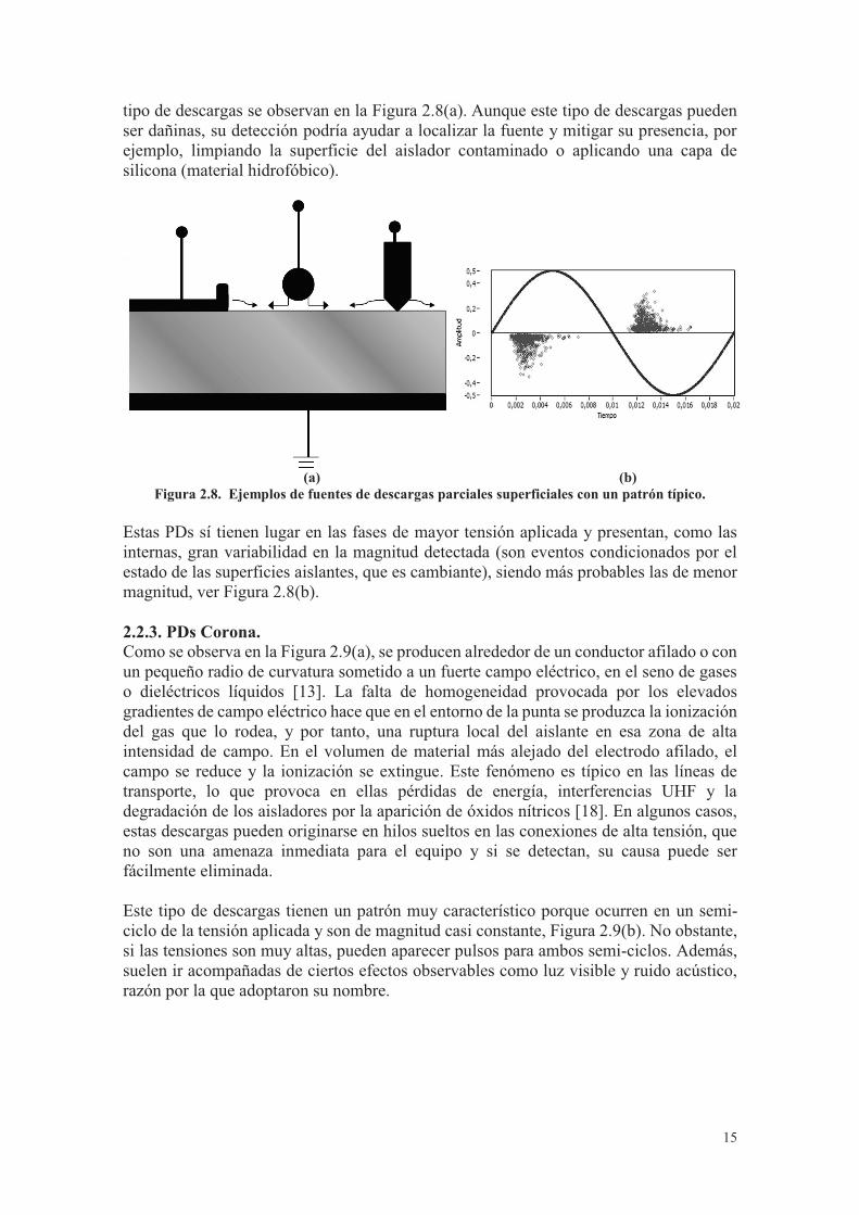
Figura 2.6. Circuito equivalente para el aislante afectado por PDs ..................... 13 Figura 2.7. Inclusión cilíndrica dieléctrica en el seno de otro dieléctrico sólido 14 Figura 2.8. Ejemplos de fuentes de descargas parciales superficiales con un

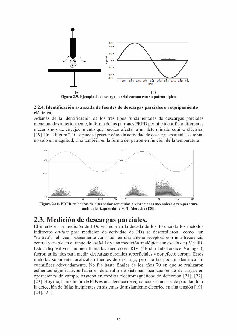
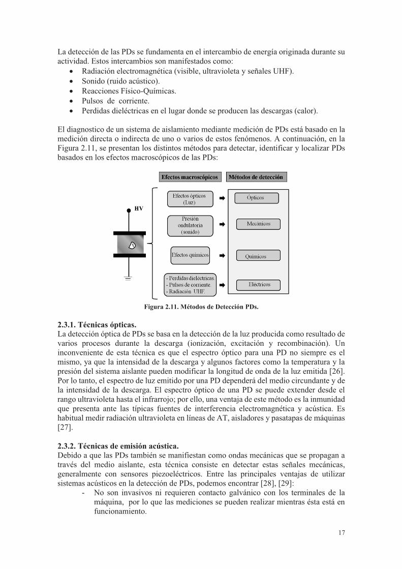
patrón típico ......................................................................................................... 15 Figura 2.9. Ejemplo de descarga parcial corona con su patrón típico ................. 16 Figura 2.10. PRPD en barras de alternador sometidas a vibraciones mecánicas a

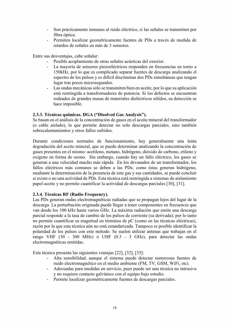
temperatura ambiente (izquierda) y 80ºC (derecha) ........................................... 16 Figura 2.11. Métodos de Detección PDs ............................................................. 17 Figura 2.12. Esquema general de un sistema de medida RF ............................... 19 Figura 2.13. Circuitos básicos de medición ......................................................... 19 Figura 2.14. Circuito Eléctrico de un sensor inductivo ....................................... 22 Figura 2.15. Función de transferencia de un sensor inductivo ............................ 22 Figura 2.16. Transformador de alta frecuencia comercial ................................... 23 Figura 2.17. Esquema de una RC experimental ................................................... 23 Figura 2.18. Sensor ILS: Esquema general .......................................................... 24 Figura 2.19. Sensor ILS: Prototipo experimental ................................................ 24 Figura 3.1. Patrones PRPD con múltiples fuentes de PDs y ruido ...................... 34 Figura 3.2. Ubicación de los condensadores por fase para separar PDs del ruido

eléctrico ................................................................................................................ 35 Figura 3.3. Filtros de descomposición ................................................................. 36 Figura 3.4. Proceso de descomposición iterativo ................................................ 37 Figura 3.5. Patrón PRPD detectado en las barras Roebel conectadas al estator, en

una configuración para generar múltiples fuentes de PDs ................................... 37 Figura 3.6. Mapa 3D que se obtiene al representar los componentes principales

de energía de los coeficientes wavelet ................................................................. 38 Figura 3.7. Sub-patrones y señales representativas para los tres clusters de la

Figura 3.6: (a), (c) y (e) sub-patrones PRPD de los clusters #1, #2 y #3 respectivamente; (b), (d) y (f) señales representativas de cada clúster ................ 39

Figura 3.8. Ejemplo de separación de fuentes usando mapas T-F ....................... 40 Figura 3.9. Datos obtenidos en un transformador de alta tensión ....................... 41 Figura 3.10(a), (b) y (c): Patrones PRPD obtenidos después de la separación de

las fuentes presentes en la Figura 3.9 ................................................................. 41 Figura 3.11. Mapa T-F para un ensayo realizado a un hidro-generador .............. 42 Figura 3.12. Componentes del modelo SVM. ..................................................... 44

Figura 3.13: Hiperplanos. (a) Rango de posibles hiperplanos, (b) Único hiperplano óptimo y su margen ........................................................................... 44

Figura 3.14. Mapeo de las muestras de entrenamiento desde el espacio de entrada al espacio característico ....................................................................................... 46

Figura 3.15. Diagrama esquemático del circuito de medición de PDs ................ 48 Figura 3.16. Objetos de ensayo utilizados para generar PDs ............................... 50 Figura 4.1. Esquema del circuito indirecto de detección de PDs utilizado ......... 54 Figura 4.2. Diagrama esquemático del sistema de adquisición ........................... 55 Figura 4.3. Programación y configuración de la etapa de adquisición ................ 56 Figura 4.4. Forma de onda típica de PD .............................................................. 57 Figura 4.5. Esquema general del algoritmo utilizado en la detección de amplitud,

polaridad y fase de los pulsos de PDs .................................................................. 57 Figura 4.6. Ejemplo de identificación de picos máximos y mínimos en un pulso

de PD .................................................................................................................... 58 Figura 4.7. Descripción de las pantallas graficas del panel principal del software.

............................................................................................................................. 59 Figura 4.8. Visualización de patrones PRPD. ...................................................... 59 Figura 4.9. Forma de onda de un pulso de PD. .................................................... 60 Figura 4.10. Espectro en frecuencia de un pulso de PD ...................................... 61 Figura 4.11. (a) Ejemplo de mapa PRH-PRL, (b) Ejemplo de selección de

intervalos de frecuencia en el espectro de las señales ......................................... 62 Figura 4.12. Visualización de parámetros estadísticos de la adquisición. ........... 63 Figura 4.13. Interfaz de usuario del sistema de adquisición de PDs ................... 64 Figura 4.14. Interfaz de usuario del software de procesamiento de PDs. Ventana

“CARGAR DATOS” .......................................................................................... 66 Figura 4.15. Interfaz de usuario del software de procesamiento de PDs. Ventana

“FILTRAR” ........................................................................................................ 67 Figura 4.16. Visualización del mapa PR, patrón PRPD y parámetros estadísticos

de las nubes de puntos asociadas a PDs corona tras filtrado de ruido ................. 69 Figura 4.17. Visualización del mapa PR, patrón PRPD y parámetros estadísticos

de la nube de puntos asociada ruido eléctrico tras filtrado de las descargas ....... 69 Figura 4.18. Interfaz de usuario del software de procesamiento de PDs. Ventana

“PRPD FILTRADO” .......................................................................................... 70 Figure 5.1. Power-ratio map regions ................................................................... 74 Figure 5.2. Experimental Setup ........................................................................... 75 Figure 5.3. Surface PDs source. Contaminated ceramic bushing (Experiment # 1)

............................................................................................................................. 76 Figure 5.4. Internal PDs source. Insulating sheets immersed in mineral oil

(experiment # 2) .................................................................................................. 77 Figure 5.5. Corona PDs source. Point-plane experimental specimen (experiment

# 3) ...................................................................................................................... 77 Figure 5.6. Surface PDs. PRPD patterns (left) and power ratio maps (right) ...... 78 Figure 5.7. Power ratio map for internal PDs. Low trigger level (800 V). Sheet

configuration 3+5+3 ............................................................................................ 80 Figure 5.8. Power ratio maps for internal PDs with different void heights. High

trigger level (10 kV) ........................................................................................... 80 Figure 5.9. Power ratio maps for internal PDs with different void heights. Low

trigger level (10 kV) ........................................................................................... 81 Figure 5.10. Corona PDs. PRPD pattern (left) and power ratio map (right). Low

trigger level (3.2 kV) .......................................................................................... 81

XIII

Figure 5.11. Summary of the power ratio maps for the different types of PDs and noise ..................................................................................................................... 82

Figure 6.1. Power ratio representation ................................................................ 88 Figure 6.2. Experimental Setup ........................................................................... 89 Figure 6.3. Test objects for corona PD ................................................................ 89 Figure 6.4. PRPD pattern (a) and PR map (b) for corona discharges .................. 90 Figure 6.5. PRPD pattern (a) and PR map (b) for internal discharges ................ 91 Figure 6.6. PRPD pattern for simultaneous internal and corona discharges.

Arrows point to PD pulses incompatible with internal PD .................................. 91 Figure 6.7. PR map for simultaneous internal and corona discharges ................. 92 Figure 6.8. PRPD pattern (a) and PR map (b) for surface discharges ................. 92 Figure 6.9. PRPD pattern (a) and PR map (b) for internal discharges ................ 93 Figure 6.10. PRPD pattern (a) and PR map (b) for simultaneous internal and

surface discharges ................................................................................................ 93 Figure 6.11. Typical frequency domain (FFT magnitude versus frequency) of

detected pulses for simultaneous internal and surface discharges ....................... 94 Figure 6.12. PR maps for internal discharges (a) and surface discharges (b).

Frequency intervals for the power ratios calculations: f1L=0 MHz, f2L= 5 MHz, f1H =25 MHz, and f2H= 29 MHz ................................................................................ 94

Figure 6.13. PR map for simultaneous internal and surface PD activity. Frequency intervals for the power ratios calculations: f1L=0 MHz, f2L= 5 MHz, f1H =25 MHz, and f2H= 29 MHz ................................................................................ 95

Figure 6.14. PRPD pattern (a) and PR map (b) for a 12/20 kV power cable ...... 95 Figure 6.15. PRPD pattern (a) and PR map (b) for corona discharges at 12 kV . 96 Figure 6.16. PRPD pattern (a) and PR map (b) for simultaneous discharges from

the power cable and corona source ...................................................................... 96 Figure 6.17. Typical frequency-domain (FFT magnitude versus frequency) of the

detected pulses for the power cable connected to the corona source setup ......... 97 Figure 6.18. PRPD pattern (a) and PR map (b) for simultaneous discharges from

the power cable and corona source. Frequency intervals for the power ratios calculations: f1L=0 MHz, f2L= 7 MHz, f1H =15 MHz, and f2H= 28 MHz .............. 97

Figure 6.19. PRPD pattern (a) and PR map (b) for simultaneous discharges from the power cable and corona source. Frequency intervals for the power ratio calculations: f1L=5 MHz, f2L= 15 MHz, f1H =10 MHz, and f2H= 25 MHz ............ 98

Figure 7.1. Experimental setup for PD measurements ...................................... 103 Figure 7.2. Devices under test: (a) Point-plane experimental specimen (b)

Contaminated ceramic bushing, (c) Pierced insulating sheets ........................... 103 Figure 7.3. Two inductive sensors. (a) HFCT and (b) ILS ................................ 105 Figure 7.4. Equivalent circuit of inductive sensors ........................................... 105 Figure 7.5. Experimental setups to obtain the frequency response of the sensors:

HFCT and ILS ................................................................................................... 106 Figure 7.6. Experimental frequency response of the HFCT .............................. 106 Figure 7.7. ILS schematic and ........................................................................... 106 Figure 7.8. Experimental frequency and derivative response of the ILS .......... 107 Figure 7.9. Power ratio representation ............................................................... 108 Figure 7.10. Schematic diagram of the procedure ............................................. 109 Figure 7.11. Corona PD. (a) PR map of the signals measured with the HFCT, (b)

Normalized average spectral power of the signals measured with the HFCT, (c) PR map of the signals measured with the ILS, (d) Normalized average spectral power of the signals measured with the ILS ...................................................... 111

Figure 7.12. Surface PD. (a) PR map of the signals measured with the HFCT, (b) Normalized average spectral power of the signals measured with the HFCT, (c) PR map of the signals measured with the ILS, (d) Normalized average spectral power of the signals measured with the ILS ...................................................... 112

Figure 7.13. Internal PD. (a) PR map of the signals measured with the HFCT, (b) Normalized average spectral power of the signals measured with the HFCT, (c) PR map of the signals measured with the ILS, (d) Normalized average spectral power of the signals measured with the ILS ...................................................... 113

Figure 7.14. PR maps for PD (cluster 1) and noise (cluster 2) obtained with both sensors ................................................................................................................ 114

Figure 7.15. Complete PRPD pattern (Left), PR map (Center) and filtered PRPD pattern (Right) obtained with the ILS sensor for (a) corona discharges and (b) internal discharges ............................................................................................. 115

Figure 8.1. Example of PR map for two pulse sources (PD and noise) ............ 121 Figure 8.2. Diagram for calculation of distances between clusters ................... 123 Figure 8.3. Frequency bands movement along BW to calculate PR (up) and

example of PR=PR(fcn,i) (down) for four detected pulses ................................ 124 Figure 8.4. Selection of the frequencies for PRH and PRL calculation for band n

........................................................................................................................... 125 Figure 8.5. Flowchart for the presented algorithm ............................................ 126 Figure 8.6. Experimental Setup ......................................................................... 127 Figure 8.7. PR maps for PD (cluster 1) and noise (cluster 2) obtained for corona

source using intervals option 1 (up), 2 (center) and 3 (down) .......................... 128 Figure 8.8. PRPD for corona PD and noise acquisition..................................... 129 Figure 8.9. Standard deviation of the power ratios for corona PD and noise when

n=7 ..................................................................................................................... 130 Figure 8.10. Power ratio map for corona and noise when the maximum MD is

obtained (left). PRPD for pulses of cluster 1 (right) ......................................... 130 Figure 8.11. Average spectra for corona PD (grey) and noise (black) pulses

measured independently .................................................................................... 131 Figure 8.12. PRPD for internal PD and noise acquisition ................................. 131 Figure 8.13. Standard deviation of the power ratios for internal PD and noise

when n=9............................................................................................................ 132 Figure 8.14. Power ratio map for internal PD and noise when the maximum MD

is obtained (left). PRPD for pulses of cluster 1 (right) ...................................... 132 Figure 8.15. Average spectra for internal PD (grey) and noise (black) pulses

measured independently .................................................................................... 133 Figure 8.16. Standard deviation of the power ratios for surface PD and noise

when n=6............................................................................................................ 133 Figure 8.17. Power ratio map for surface PD and noise when the maximum MD

is obtained (left). PRPD for pulses of cluster 1 (right) ..................................... 134 Figure 8.18. Average spectra for surface PD (grey) and noise (black) pulses

measured independently .................................................................................... 134 Figure 8.19. PRPD patterns for corona PD (left) and internal PD (right) for

independent experiments. Applied voltage, 4.7 kV ........................................... 135 Figure 8.20. PRPD pattern for simultaneous corona and internal PD. Applied

voltage, 4.7 kV ................................................................................................... 135 Figure 8.21. Standard deviation of the power ratios for corona and internal PD

when n=5............................................................................................................ 136

XV

Figure 8.22. PR maps for intervals option 3 (left) and those selected from the algorithm (right) ................................................................................................ 136

Figure 8.23. PRPD patterns for corona PD (left) and internal PD (right) filtered after cluster selection (algorithm). Simultaneous applied voltage for both objects, 4.7kV .................................................................................................................. 136

Figure 8.24. Average spectra for corona PD (black) and internal PD (grey) pulses measured independently .................................................................................... 137

Figure 8.25. PRPD patterns for surface PD (left) and internal PD (right) for independent experiments. Applied voltage, 10 kV ............................................ 137

Figure 8.26. PRPD pattern for simultaneous surface and internal PD. Applied voltage, 10 kV. .................................................................................................. 138

Figure 8.27. Standard deviation of the power ratios for surface and internal PD when n=3............................................................................................................ 138

Figure 8.28. PR maps for intervals option 2 (left) and those selected from the algorithm (right) ................................................................................................ 139

Figure 8.29. PRPD patterns for internal PD (left) and surface PD (right) filtered after cluster selection (algorithm). Simultaneous applied voltage for both objects, 10 kV .................................................................................................................. 139

Figure 8.30. Average spectra for internal PD (grey) and surface PD (black) pulses measured independently .................................................................................... 139

Figure 8.31. PRPD pattern for discharges in the power cable and noise acquisition .......................................................................................................... 140

Figure 8.32. Average spectra for PD (grey) and noise (black) pulses measured independently ..................................................................................................... 141

Figure 8.33. Power ratio map for PD and noise in the power cable when the maximum MD is obtained (left). PRPD for pulses of cluster 1 (right) ............. 141

Figure 8.34. PRPD patterns for corona PD (left) and partial discharges measured in the power cable (right) for independent experiments. Applied voltage, 9 kV141

Figure 8.35. PRPD pattern for discharges from power cable and corona source acquisition .......................................................................................................... 142

Figure 8.36. Power ratio map for discharges from power cable (cluster 1) and corona source (cluster 2) in a simultaneous acquisition. n=8 ............................ 142

Figure 8.37. PRPD patterns for corona PD (left) and discharges from power cable (right) filtered after cluster selection (algorithm). Simultaneous applied voltage for both objects, 9 kV ........................................................................................ 143

Figure 8.38. Average spectra for discharges from power cable (grey) and corona PD (black) pulses measured independently ....................................................... 143

XVII

Lista de Tablas

Tabla 4.1. Rendimiento del sistema (%) basado en una SVM Multi-Clase para diferentes niveles de presión de gas. Fuente ..................................................... 50

Table 7.1. Trigger and voltage levels to characterize noise, PD and PD + noise ........................................................................................................................ 104

Table 7.2. Parameters of the used ILS ............................................................ 107 Table 7.3. MD and ED between clusters obtained with the two sensors for the

intervals PRL [10, 30] MHz and PRH [30, 50] MHz ..................................... 116 Table 7.4. MD and ED between clusters obtained with the two sensors for the

intervals. PRL [0, 20] MHz and PRH [20, 40] MHz ...................................... 116 Table 7.5. MD and between clusters obtained with the two sensors for the

intervals. PRL [20, 40] MHz and PRH [40, 60] MHz .................................... 117 Table 8.1. Mahalanobis distance between clusters in simultaneous acquisition

of PD and noise ............................................................................................... 128 Table 8.2. Selected frequencies by the algorithm for corona and noise data . 129 Table 8.3. Mahalanobis distance between clusters in simultaneous acquisition

of corona and internal PD ............................................................................... 135 Table 8.4. Mahalanobis distance between clusters in simultaneous acquisition

of surface and internal PD .............................................................................. 138 Table 8.5. Mahalanobis distance between clusters in simultaneous acquisition

of PD and noise in the insulated power cable ................................................. 140 Table 8.6. Mahalanobis distance between clusters in simultaneous acquisition

of PD in the insulated power cable and corona .............................................. 142

XIX

Agradecimientos A Dios, por permitir el cumplimiento de este sueño. A Paula mi amada esposa, por su comprensión, amor y apoyo incondicional. A David mi hijo y más preciado tesoro, por alegrarme la vida y hacerme el padre más feliz del mundo. A mi madre y hermanas, porque nunca se han cansado de darme una mano en los momentos difíciles. A Juan Manuel, por darme la oportunidad desde el primer momento, por su infinita paciencia e incansable dedicación. A Guillermo, Ángel y Emilio por sus valiosos aportes y concejos en todo momento. Y finalmente, a todas aquellas personas que tengo el honor de llamar “amigos”… ellos saben quiénes son.

XXI

Resumen

En entornos industriales o incluso en ambientes controlados como laboratorios de alta tensión, los impulsos procedentes de múltiples fuentes de Descargas Parciales (PDs) y ruido eléctrico se pueden superponer llegando modificar y alterar los resultados de las mediciones de PDs conduciendo finalmente a interpretaciones erróneas. Asimismo, algunos tipos de descargas, como es el caso de las tipo corona o superficiales, no suelen influir algunas veces en la expectativa de vida en los sistemas aislantes, al contrario de lo que ocurre con las internas, que sí pueden llegar a causar la ruptura en un corto tiempo. Por estos motivos, la separación e identificación de fuentes de PDs y ruido se ha convertido en un requisito fundamental a la hora de obtener un diagnóstico efectivo del aislamiento y evitar así evaluaciones erróneas en equipos como máquinas eléctricas y cables aislados. El propósito de esta Tesis es la presentación de un nuevo método de separación y clasificación de fuentes de PDs y ruido basado en el análisis de la potencia espectral de los pulsos de PDs para determinadas bandas de frecuencia. Este método permite separar en un mapa 2D las diferentes fuentes que puedan estar presentes durante la adquisición, a través de nubes de puntos clusters que se ubican en diferentes partes del mapa de acuerdo a su naturaleza. Conjuntamente se presenta el desarrollo de un algoritmo que permite seleccionar de forma automática las bandas de frecuencia de mayor interés con el fin de mejorar la separación de los clusters en el mapa. Adicionalmente, una serie de experimentos realizados en varios objetos de ensayo y equipos reales son presentados, con el fin de validar el comportamiento del método de separación y del algoritmo de selección automática propuestos en este documento.

XXIII

Abstract

Both at industrial environments and even controlled facilities as high voltage laboratories the onset and overlap of Partial Discharges (PDs) and electromagnetic noise is possible which may lead to disturbances on the measurements made and entailing misleading results. Furthermore, some specific types of discharges as corona and surface PDs do not usually affect the expected lifetime of insulation systems such as occur in the case of internal discharges which frequently leads to the breakdown of the insulation in a short period of time. On those grounds the accurate identification of the PDs and its differentiation from other signals like electric noise have become a basic requirement when an effective insulation diagnosis is required avoiding erroneous results and a wrong diagnosis of electrical machines and power cables. The purpose of this thesis is to present a new method for separating and classifying PDs and noise sources by means of the analysis of the spectral power from the detected pulses for certain frequency bands. This method allows the separation in a 2D map of different sources that may be present during acquisition, through clouds of clusters that are located in different parts of the map according to their nature. In addition it has been developed an algorithm for the automatic selection of the frequency bands of interest in order to improve the separation of the clusters on the map. Additionally, a series of experiments conducted on various test objects and real high voltage equipment are presented, in order to validate the performance of the separation method and the algorithm for the automatic selection of frequency intervals that is proposed in this document.

1

Capítulo 1 Introducción

Contenidos 1.1. Motivación de la Tesis ............................................................................................... 1 1.2. Finalidad y objetivos de la Tesis ............................................................................... 4 1.3. Estructura de la Tesis ................................................................................................. 5 Bibliografia ....................................................................................................................... 6

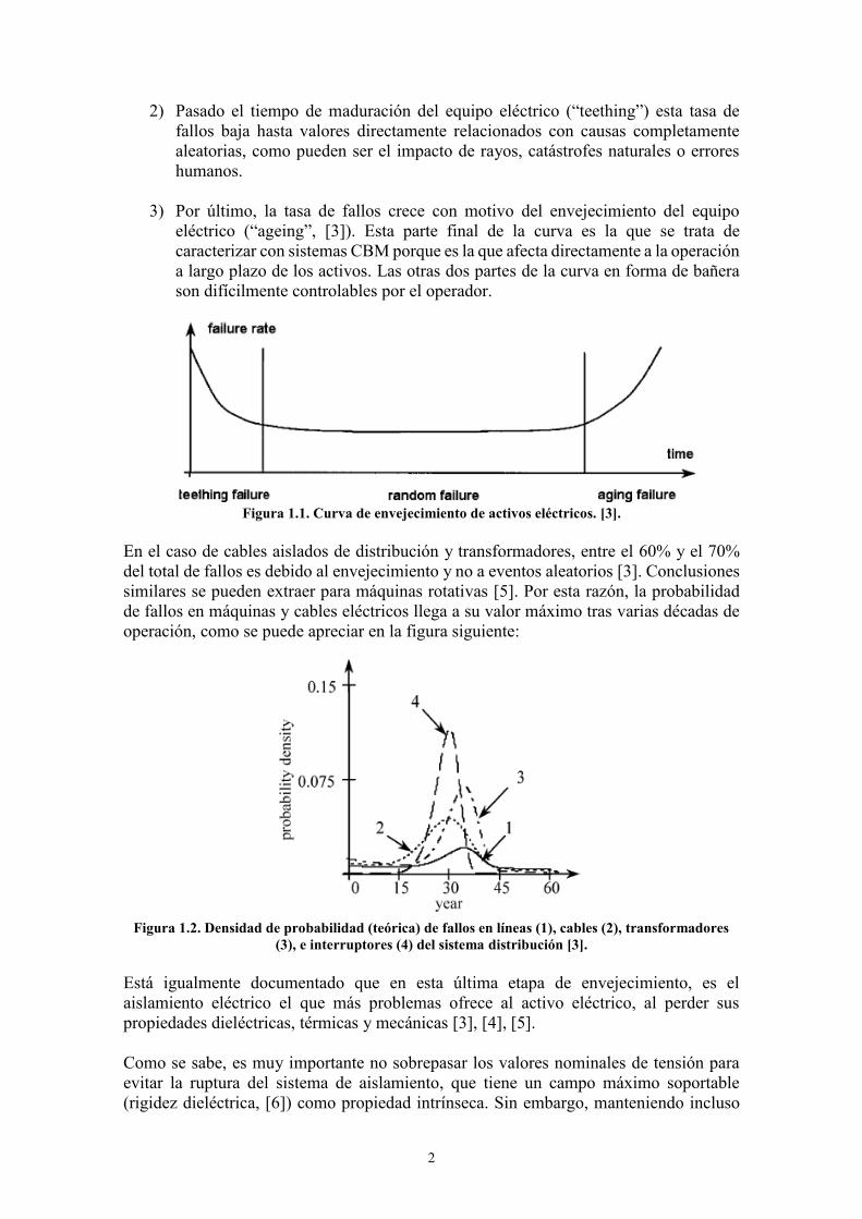
1.1. Motivación de la Tesis. Las infraestructuras eléctricas de generación, transporte e incluso distribución requieren de grandes inversiones económicas, por lo que su rentabilidad a largo plazo debe ser optimizada. En este contexto, ha crecido el interés, por un lado, en reducir los periodos de mantenimiento de máquinas y cables eléctricos cuando se encuentren muy envejecidos, y por otro, en planificar adecuadamente su reemplazo cuando su operación no es fiable [1]. En muchas empresas dedicadas al transporte y la distribución, se da por hecho que los equipos eléctricos deben ser reemplazados cada cierto tiempo (en torno a 30-40 años, [2], [3]), y que los periodos de mantenimiento deben estar fijados de antemano (mantenimiento preventivo). No obstante, los avances obtenidos de la investigación básica respecto al aislamiento eléctrico y el incremento de los datos accesibles sobre históricos de fallos permiten apostar por nuevas estrategias en las que el conocimiento de las condiciones de operación del activo eléctrico, y las medidas en servicio (on-line) que se puedan hacer en el mismo, permitirían alargar tanto la esperanza de vida del equipo, como sus periodos de mantenimiento programado [4]. De esta forma, la falta de inversión que suele ser necesaria en el reemplazo de equipos [3] podría ser compensada con cierto margen de seguridad ofrecido por este mantenimiento basado en condición (“Condition-Based Maintenance”, CBM). La experiencia en el estudio de probabilidades de fallo de máquinas y cables aislados, apunta a un comportamiento con “forma de bañera” durante su vida útil. Tal y como se ve en la Figura 1.1, esta tasa de fallos decrece hasta llegar a un valor estable en la “madurez” del activo, para luego incrementarse de nuevo [3]. Los fallos en cada etapa se asocian a diversos fenómenos:

1) En los primeros años de vida del activo, los fallos se deben a errores de fabricación o instalación del equipo. No deberían ser muy significativos y en algunos casos, pueden quedar cubiertos por garantías de fabricante.

2

2) Pasado el tiempo de maduración del equipo eléctrico (“teething”) esta tasa de fallos baja hasta valores directamente relacionados con causas completamente aleatorias, como pueden ser el impacto de rayos, catástrofes naturales o errores humanos.

3) Por último, la tasa de fallos crece con motivo del envejecimiento del equipo

eléctrico (“ageing”, [3]). Esta parte final de la curva es la que se trata de caracterizar con sistemas CBM porque es la que afecta directamente a la operación a largo plazo de los activos. Las otras dos partes de la curva en forma de bañera son difícilmente controlables por el operador.

Figura 1.1. Curva de envejecimiento de activos eléctricos. [3].

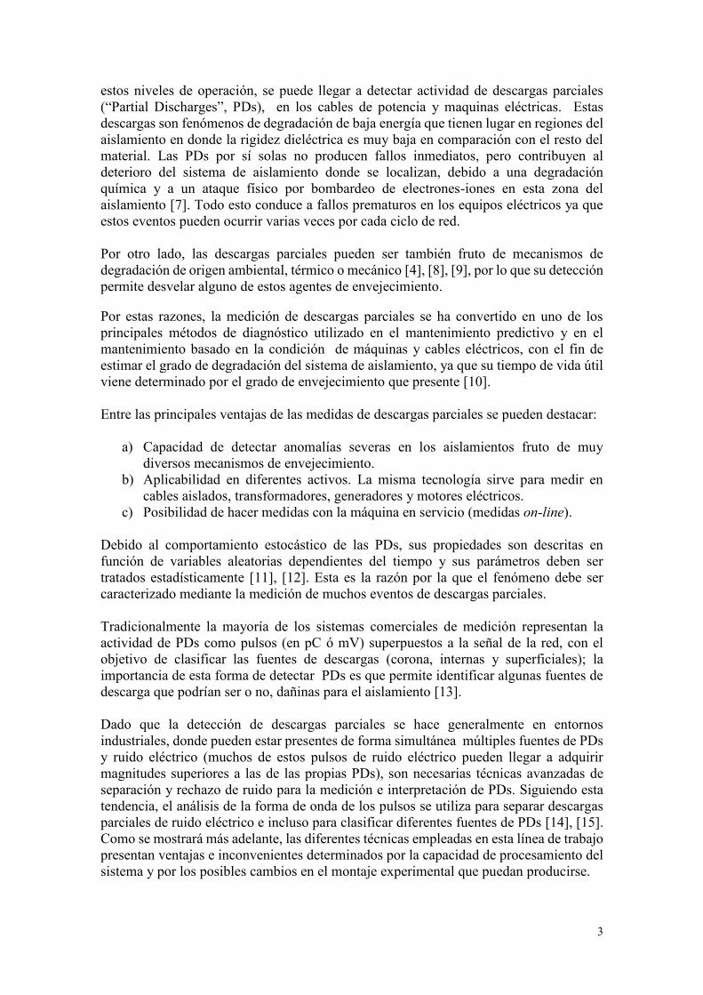
En el caso de cables aislados de distribución y transformadores, entre el 60% y el 70% del total de fallos es debido al envejecimiento y no a eventos aleatorios [3]. Conclusiones similares se pueden extraer para máquinas rotativas [5]. Por esta razón, la probabilidad de fallos en máquinas y cables eléctricos llega a su valor máximo tras varias décadas de operación, como se puede apreciar en la figura siguiente:

Figura 1.2. Densidad de probabilidad (teórica) de fallos en líneas (1), cables (2), transformadores

(3), e interruptores (4) del sistema distribución [3]. Está igualmente documentado que en esta última etapa de envejecimiento, es el aislamiento eléctrico el que más problemas ofrece al activo eléctrico, al perder sus propiedades dieléctricas, térmicas y mecánicas [3], [4], [5]. Como se sabe, es muy importante no sobrepasar los valores nominales de tensión para evitar la ruptura del sistema de aislamiento, que tiene un campo máximo soportable (rigidez dieléctrica, [6]) como propiedad intrínseca. Sin embargo, manteniendo incluso

3

estos niveles de operación, se puede llegar a detectar actividad de descargas parciales (“Partial Discharges”, PDs), en los cables de potencia y maquinas eléctricas. Estas descargas son fenómenos de degradación de baja energía que tienen lugar en regiones del aislamiento en donde la rigidez dieléctrica es muy baja en comparación con el resto del material. Las PDs por sí solas no producen fallos inmediatos, pero contribuyen al deterioro del sistema de aislamiento donde se localizan, debido a una degradación química y a un ataque físico por bombardeo de electrones-iones en esta zona del aislamiento [7]. Todo esto conduce a fallos prematuros en los equipos eléctricos ya que estos eventos pueden ocurrir varias veces por cada ciclo de red. Por otro lado, las descargas parciales pueden ser también fruto de mecanismos de degradación de origen ambiental, térmico o mecánico [4], [8], [9], por lo que su detección permite desvelar alguno de estos agentes de envejecimiento. Por estas razones, la medición de descargas parciales se ha convertido en uno de los principales métodos de diagnóstico utilizado en el mantenimiento predictivo y en el mantenimiento basado en la condición de máquinas y cables eléctricos, con el fin de estimar el grado de degradación del sistema de aislamiento, ya que su tiempo de vida útil viene determinado por el grado de envejecimiento que presente [10]. Entre las principales ventajas de las medidas de descargas parciales se pueden destacar:

a) Capacidad de detectar anomalías severas en los aislamientos fruto de muy diversos mecanismos de envejecimiento.

b) Aplicabilidad en diferentes activos. La misma tecnología sirve para medir en cables aislados, transformadores, generadores y motores eléctricos.

c) Posibilidad de hacer medidas con la máquina en servicio (medidas on-line). Debido al comportamiento estocástico de las PDs, sus propiedades son descritas en función de variables aleatorias dependientes del tiempo y sus parámetros deben ser tratados estadísticamente [11], [12]. Esta es la razón por la que el fenómeno debe ser caracterizado mediante la medición de muchos eventos de descargas parciales. Tradicionalmente la mayoría de los sistemas comerciales de medición representan la actividad de PDs como pulsos (en pC ó mV) superpuestos a la señal de la red, con el objetivo de clasificar las fuentes de descargas (corona, internas y superficiales); la importancia de esta forma de detectar PDs es que permite identificar algunas fuentes de descarga que podrían ser o no, dañinas para el aislamiento [13]. Dado que la detección de descargas parciales se hace generalmente en entornos industriales, donde pueden estar presentes de forma simultánea múltiples fuentes de PDs y ruido eléctrico (muchos de estos pulsos de ruido eléctrico pueden llegar a adquirir magnitudes superiores a las de las propias PDs), son necesarias técnicas avanzadas de separación y rechazo de ruido para la medición e interpretación de PDs. Siguiendo esta tendencia, el análisis de la forma de onda de los pulsos se utiliza para separar descargas parciales de ruido eléctrico e incluso para clasificar diferentes fuentes de PDs [14], [15]. Como se mostrará más adelante, las diferentes técnicas empleadas en esta línea de trabajo presentan ventajas e inconvenientes determinados por la capacidad de procesamiento del sistema y por los posibles cambios en el montaje experimental que puedan producirse.

4

Siguiendo con esta línea de investigación, esta Tesis tiene como motivación el desarrollo de un nuevo método de separación de fuentes de PDs y ruido basado en el cálculo de la relación de potencia espectral en alta y baja frecuencia de cada uno de los pulsos detectados. La representación de la potencia espectral relativa de estos dos intervalos de frecuencia en un mapa bidimensional permite identificar claramente agrupaciones diferenciadas de cada uno de los efectos de PDs y ruido, lo que facilita su análisis por separado. Posteriormente, mediante los diagramas clásicos fase-amplitud, se puede identificar cada una de esas agrupaciones (clusters) y así evaluar su situación, lo que permite diagnosticar el estado de deterioro del aislamiento. Por otro lado, las bandas de frecuencia analizadas se pueden variar de acuerdo a lo que el usuario esté observando durante la adquisición. Esto hace que la técnica sea más flexible que la utilizada por otros sistemas a la hora de separar agrupaciones en un mapa de clasificación. Además, con la implementación de un algoritmo de selección automática de intervalos (también presentada en esta Tesis), se garantiza que el sistema aporte intervalos adecuados para una buena separación. 1.2. Finalidad y objetivos de la Tesis. La finalidad de esta Tesis es implementar un novedoso método de separación y clasificación de fuentes de PDs y ruido, basado en el análisis de las relaciones de potencia espectral para bandas de frecuencia (altas y bajas) en cada pulso de PD. Estas bandas de frecuencia pueden ser seleccionadas manualmente de acuerdo a lo observado en el espectro de cada señal y sus correspondientes potencias relativas representadas en un mapa bidimensional (en 2D). Este nuevo método de separación deberá ser implementado en un sistema de detección y probado en varios objetos de ensayo y equipos reales; igualmente, debe ser compatible con diversos sensores. Adicionalmente se plantea el desarrollo de un algoritmo para la selección automática de las bandas de frecuencia con el fin de obtener mejores resultados (en términos de separación), que los obtenidos al seleccionar las bandas de forma manual. Para llevar a cabo lo descrito anteriormente, se definen los siguientes objetivos específicos:

Revisión del estado del arte sobre técnicas de separación e identificación de descargas parciales y ruido eléctrico.

Implementar en un sistema de adquisición de descargas parciales la técnica de agrupación propuesta en esta Tesis, que permita separar y filtrar los cluster asociados a descargas parciales y ruido. Este sistema se programará para identificar fuentes off-line tras grabación previa de datos y con Alta Tensión aplicada on-line.

Cuantificar la capacidad de separación de fuentes de Descarga Parcial y Ruido

entre diferentes sensores inductivos a través de medidas realizadas a diferentes objetos de ensayo.

Implementar un algoritmo que permita aumentar automáticamente las distancias

entre los clusters en función de los intervalos de frecuencia evaluados.

5

1.3. Estructura de la Tesis. El desarrollo del documento comienza en el Capítulo 1 con una descripción general del contenido de la Tesis. En el Capítulo 2, se hace una introducción al fenómeno de las descargas parciales, sus causas y consecuencias sobre el envejecimiento del sistema de aislamiento. A continuación se definen los tipos de PDs según su origen y los métodos de medición utilizados de acuerdo a los efectos macroscópicos de las mismas. Por último se describen los diferentes parámetros estadísticos usados en la identificación de fuentes de PDs y su implementación en sistemas expertos con el fin de realizar de manera automática una identificación del tipo de fuente de PD. En el Capítulo 3 se hace una profunda revisión del estado del arte de los más importantes métodos de separación de fuentes de PDs y ruido que se han implementado de manera experimental e industrial. En el Capítulo 4 se describe el sistema de adquisición y pre-procesamiento PD_LINEALT y el software off-line de procesamiento LINEALT_PROCESSING, los cuales se han desarrollado a lo largo de esta Tesis con el fin de implementar e integrar la técnica de separación propuesta. El Capítulo 5 se inicia con la presentación y descripción de la técnica de separación propuesta, la cual se basa en el análisis de la potencia espectral de los pulsos de PDs para bandas de frecuencia altas y bajas. Seguidamente se presentan los resultados obtenidos con esta nueva técnica a la hora de separar diversas fuentes de descargas parciales de ruido eléctrico superpuesto. En el Capítulo 6 se analiza la capacidad de separación de la técnica propuesta, modificando las bandas de frecuencia, con el fin de mejorar la separación de las nubes de puntos que se obtienen cuando están activas simultáneamente múltiples fuentes de PDs. En el Capítulo 7 se presentan los resultados de la separación de clusters asociados a fuentes de PDs y ruido utilizando la técnica de separación propuesta para dos sensores inductivos diferentes. Adicionalmente la capacidad de separación para estos dos sensores es medida a través de dos métricas diferentes: distancia Euclídea y distancia Mahalanobis. Finalmente, en el Capítulo 8 se presenta el desarrollo de un algoritmo que permite obtener de forma automática las bandas de frecuencia de mayor interés, en función de la dispersión estadística de la potencia espectral relativa de las señales bajo análisis. Los resultados del algoritmo son comparados con los resultados que se obtienen al seleccionar las bandas de frecuencia manualmente, además de aplicarse a un ensayo con un equipo real. Hay que señalar al lector de este documento, que los Capítulos 5, 6, 7 y 8 pueden ser leídos independientemente ya que cada uno corresponde a los resultados obtenidos secuencialmente en el desarrollo de esta Tesis. Éstos han sido escritos como artículos y se han publicado en diferentes revistas indexadas en el Journal Citations Report de Thomson-Reuters. El Capítulo 8 aún se encuentra en etapa de revisión por parte de la revista.

6

Las conclusiones, aportaciones y publicaciones realizadas se encuentran en el Capítulo 9. Bibliografía.

1. Willis H., R. R. Schrieber.; “Aging power delivery infrastructures”; 2nd edition; CRC Press, 2013.

2. R. Gorur, W. Jewell; “A Novel Approach for Prioritizing Maintenance of Underground Cables”; Power Systems Engineering Research Center, PSERC Publication 06-40; 2006.

3. Zhang X., Gockenbach E., Wasserberg V., Borsi H.; “Estimation of the Lifetime of the Electrical Components in Distribution networks”; IEEE Transactions on Power Delivery; Vol. 22, nº1, pp 515-522; 2007.

4. James R. E, Su G; “Condition assessment of High Voltage Insulation in Power System Equipment”; The Institution of Engineering and Technology, 2008.

5. Stone G, Boutler E.A, Culbert I, Dhirani H; "Electrical Insulation for Rotating Machines: Design, Evaluation, Aging, Testing and Repair"; IEEE Press Series on Power Engineering, Wiley Interscience; 2004.

6. Kuffel E, Zaengl W.S, and Kuffel J; “High Voltage Engineering: Fundamentals”, 2nd ed.; Butterworth-Heinemann; 2000.

7. P. Morshuis, “Degradation of Solid Dielectrics due to internal partial discharge: Some thoughts on progress made and where to go now”, IEEE Trans. Dielectr. Electr. Insul., Vol. 12, pp. 905-913, 2005.

8. Kreuger F. H; “Partial Discharge Detection in High-Voltage Equipment”; Butterworths, Londres, 1989.

9. Stone G.C; “The statistics of aging models and practical reality”; Electrical Insulation, IEEE Transactions on, vol 28, pp. 716-728, Oct 1993.

10. IEC 60270; “High Voltage Test Techniques. Partial Discharge Measurements”; 3a edition, 2000.

11. Krivda A; “Recognition of Discharges Discrimination and Classification”; Delft Press, 1995.

12. Lapp A, Kranz H. G; “The use of the CIGRE data format for PD diagnosis applications”; Dielectrics and Electrical Insulation, IEEE Transactions on, vol.7, pp.102-112, Feb 2000.

13. CIGRE; “Recognition of Discharges”; Electra, 1969. 14. Okubo, H, Hayakawa N; “A novel technique for partial discharge and breakdown

investigation based on current pulse waveform analysis”; Dielectrics and Electrical Insulation, IEEE Transactions on, vol.12, pp. 736- 744, Aug. 2005.

15. Cavallini A, Montanari G, Contin A, Pulletti F; “A new approach to the diagnosis of solid insulation systems based on PD signal inference”; IEEE Electrical Insulation Magazine, vol. 19, pp. 22–30, Mar-Apr 2003.

7

Capítulo 2 Estado del arte

Contenidos 2.1. Introducción a las descargas parciales: descripción y fundamentos físicos .............. 1 2.2. Tipos de descargas parciales.................................................................................... 11 2.2.1. PDs Internas ........................................................................................................ 11 2.2.2. PDs Superficiales ................................................................................................ 14 2.2.3. PDs Corona ......................................................................................................... 15 2.2.4. Identificación avanzada de fuentes de descargas parciales en equipamiento eléctrico......................................................................................................................... 16

2.3. Medición de descargas parciales ............................................................................. 16 2.3.1. Técnicas ópticas .................................................................................................. 17 2.3.2. Técnicas de emisión acústica .............................................................................. 17 2.3.3. Técnicas químicas. DGA (“Disolved Gas Analysis”) ........................................ 18 2.3.4. Técnicas RF (Radio Frequency) ......................................................................... 18 2.3.5. Técnicas eléctricas .............................................................................................. 19 2.3.6. Sensores inductivos para la detección de PDs .................................................... 20 2.3.6.1 HFCT .............................................................................................................. 23 2.3.6.2 RC ................................................................................................................... 23 2.3.6.3 ILS .................................................................................................................. 23

2.4. Caracterización estadística de las PDs..................................................................... 24 2.4.1. Análisis estadístico de distribuciones de fase. .................................................... 25 2.4.2. Tratamiento estadístico de amplitudes y tasa de repetición de descargas parciales. ....................................................................................................................... 25 2.4.3. Identificación automática de patrones PRPD. .................................................... 27 2.4.3.1 Identificación de fuentes de PDs con algoritmos basados en lógica fuzzy (lógica difusa) ............................................................................................................. 27 2.4.3.2 Identificación de fuentes de PDs con redes neuronales:. ................................ 28

Bibliografia ..................................................................................................................... 28

2.1. Introducción a las descargas parciales: descripción y fundamentos físicos. En condiciones normales de funcionamiento, los sistemas de aislamiento de máquinas eléctricas y cables aislados pueden llegar a sufrir fallos inesperados asociados a continuos esfuerzos mecánicos, térmicos, eléctricos y ambientales [1], [2], [3]. Estos esfuerzos, con el tiempo, tienden envejecer y a degradar el aislamiento llevándolo a la pérdida definitiva de sus propiedades aislantes y por lo tanto a la ruptura total del mismo. En las etapas anteriores al fallo, es habitual detectar procesos de ionización de baja energía, (por ejemplo en el interior de pequeñas vacuolas atrapadas en el seno del material aislante o en la superficie de un dieléctrico contaminado) en donde están presentes campos eléctricos altamente divergentes; estos procesos son llamados Descargas

8

Parciales (“Partial Discharges”, PDs) y pueden considerarse como un indicador relevante del estado general del sistema de aislamiento [4], [5]. Una descarga parcial es un fenómeno de ruptura eléctrica de baja energía limitado a una región del medio aislante, entre dos conductores que se encuentran a diferente potencial [6]. La localización de la descarga es consecuencia de un incremento de campo eléctrico en una región que es relativamente pequeña comparada con las dimensiones del medio aislante total o bien por la presencia de un medio de inferior rigidez dieléctrica en el sistema de aislamiento, aunque ambas circunstancias pueden darse simultáneamente. Esta región debe estar completa o parcialmente en fase gaseosa y puede corresponder, por ejemplo, a oclusiones en aislamientos sólidos, burbujas formadas por la vaporización de un líquido o gases que rodean puntas conductoras con radios de curvatura pequeños. Por tanto, los gases (aire, H2, O2, CO2, entre otros) pueden considerarse como los ambientes propicios donde pueden originarse PDs [6]. El fenómeno de las descargas parciales se basa en procesos de disrupción de un dieléctrico gaseoso, cuyas teorías están ya muy consolidadas [7]. De su estudio se puede concluir que para que haya actividad de PDs en un sistema de aislamiento es necesario que se cumplan simultáneamente dos condiciones:

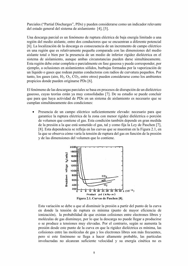
Presencia de un campo eléctrico suficientemente elevado: necesario para que garantice la ruptura eléctrica de la zona con menor rigidez dieléctrica o porción de volumen que contiene el gas. Esta condición también depende en gran medida de la presión a la que está sometido el gas, tal y como fija la Ley de Paschen [7], [8]. Esta dependencia se refleja en las curvas que se muestran en la Figura 2.1, en la que se observa cómo varía la tensión de ruptura del gas en función de la presión y de las dimensiones del volumen que lo contiene.

Figura 2.1. Curvas de Paschen [8].

Esta variación se debe a que al disminuir la presión a partir del punto de la curva en donde la tensión de ruptura es mínima (punto de mayor eficiencia de ionización), la probabilidad de que existan colisiones entre electrones libres y moléculas de gas disminuye, por lo que la descarga no puede llegar a producirse o se produce a tensiones muy elevadas. Por el contrario, según se aumenta la presión desde este punto de la curva en que la rigidez dieléctrica es mínima, las colisiones entre las moléculas de gas y los electrones libres son más frecuentes, pero si este fenómeno se llega a hacer altamente probable, las partículas involucradas no alcanzan suficiente velocidad y su energía cinética no es

10

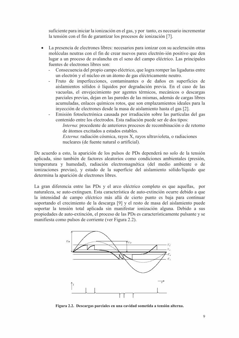
En la Figura 2.2, se representa la tensión (Ua) aplicada al conjunto del sistema de aislamiento y la tensión que cae en la zona de mayor divergencia del campo eléctrico (Uc) y menor rigidez dieléctrica. Cuando la tensión (Uc) alcanza la tensión de ignición Ui

+

(“Discharge Inception Voltage”, DIV) en el volumen eléctricamente más débil, se produce una descarga e inmediatamente la tensión Uc cae bruscamente hasta un valor (Ue) llamado tensión de extinción de descargas parciales (“Discharge Extinction Voltage”, DEV) formándose así una corriente transitoria. Tras la descarga, el aislamiento en la cavidad se ve sometido a la tensión creciente de la fuente que aumenta progresivamente intentando seguirla. El aumento de la tensión provoca otra descarga cuando se alcanza nuevamente el nivel de la tensión de ignición Ui

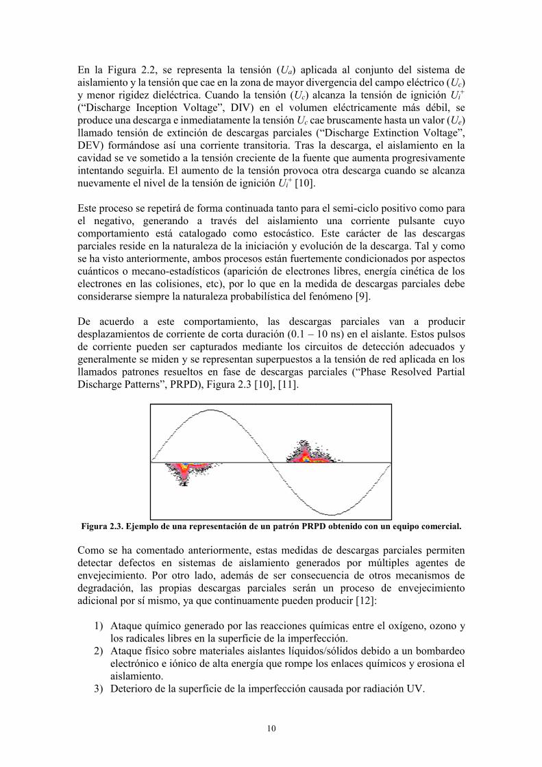
+ [10]. Este proceso se repetirá de forma continuada tanto para el semi-ciclo positivo como para el negativo, generando a través del aislamiento una corriente pulsante cuyo comportamiento está catalogado como estocástico. Este carácter de las descargas parciales reside en la naturaleza de la iniciación y evolución de la descarga. Tal y como se ha visto anteriormente, ambos procesos están fuertemente condicionados por aspectos cuánticos o mecano-estadísticos (aparición de electrones libres, energía cinética de los electrones en las colisiones, etc), por lo que en la medida de descargas parciales debe considerarse siempre la naturaleza probabilística del fenómeno [9]. De acuerdo a este comportamiento, las descargas parciales van a producir desplazamientos de corriente de corta duración (0.1 – 10 ns) en el aislante. Estos pulsos de corriente pueden ser capturados mediante los circuitos de detección adecuados y generalmente se miden y se representan superpuestos a la tensión de red aplicada en los llamados patrones resueltos en fase de descargas parciales (“Phase Resolved Partial Discharge Patterns”, PRPD), Figura 2.3 [10], [11].

Figura 2.3. Ejemplo de una representación de un patrón PRPD obtenido con un equipo comercial.

Como se ha comentado anteriormente, estas medidas de descargas parciales permiten detectar defectos en sistemas de aislamiento generados por múltiples agentes de envejecimiento. Por otro lado, además de ser consecuencia de otros mecanismos de degradación, las propias descargas parciales serán un proceso de envejecimiento adicional por sí mismo, ya que continuamente pueden producir [12]:

1) Ataque químico generado por las reacciones químicas entre el oxígeno, ozono y los radicales libres en la superficie de la imperfección.

2) Ataque físico sobre materiales aislantes líquidos/sólidos debido a un bombardeo electrónico e iónico de alta energía que rompe los enlaces químicos y erosiona el aislamiento.

3) Deterioro de la superficie de la imperfección causada por radiación UV.

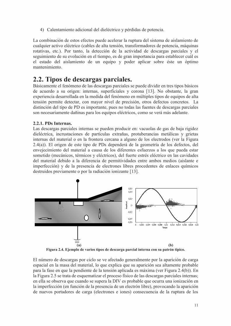
12

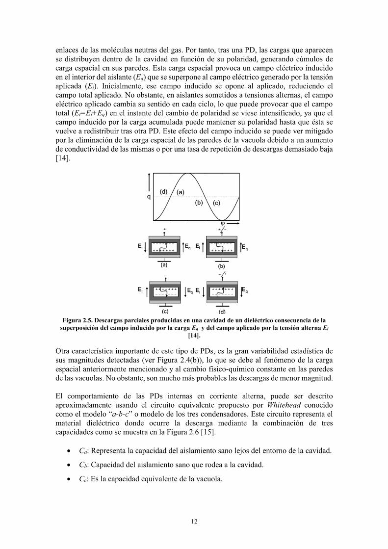
enlaces de las moléculas neutras del gas. Por tanto, tras una PD, las cargas que aparecen se distribuyen dentro de la cavidad en función de su polaridad, generando cúmulos de carga espacial en sus paredes. Esta carga espacial provoca un campo eléctrico inducido en el interior del aislante (Eq) que se superpone al campo eléctrico generado por la tensión aplicada (Ei). Inicialmente, ese campo inducido se opone al aplicado, reduciendo el campo total aplicado. No obstante, en aislantes sometidos a tensiones alternas, el campo eléctrico aplicado cambia su sentido en cada ciclo, lo que puede provocar que el campo total (Et=Ei+Eq) en el instante del cambio de polaridad se viese intensificado, ya que el campo inducido por la carga acumulada puede mantener su polaridad hasta que ésta se vuelve a redistribuir tras otra PD. Este efecto del campo inducido se puede ver mitigado por la eliminación de la carga espacial de las paredes de la vacuola debido a un aumento de conductividad de las mismas o por una tasa de repetición de descargas demasiado baja [14].

Figura 2.5. Descargas parciales producidas en una cavidad de un dieléctrico consecuencia de la

superposición del campo inducido por la carga Eq y del campo aplicado por la tensión alterna Ei [14].

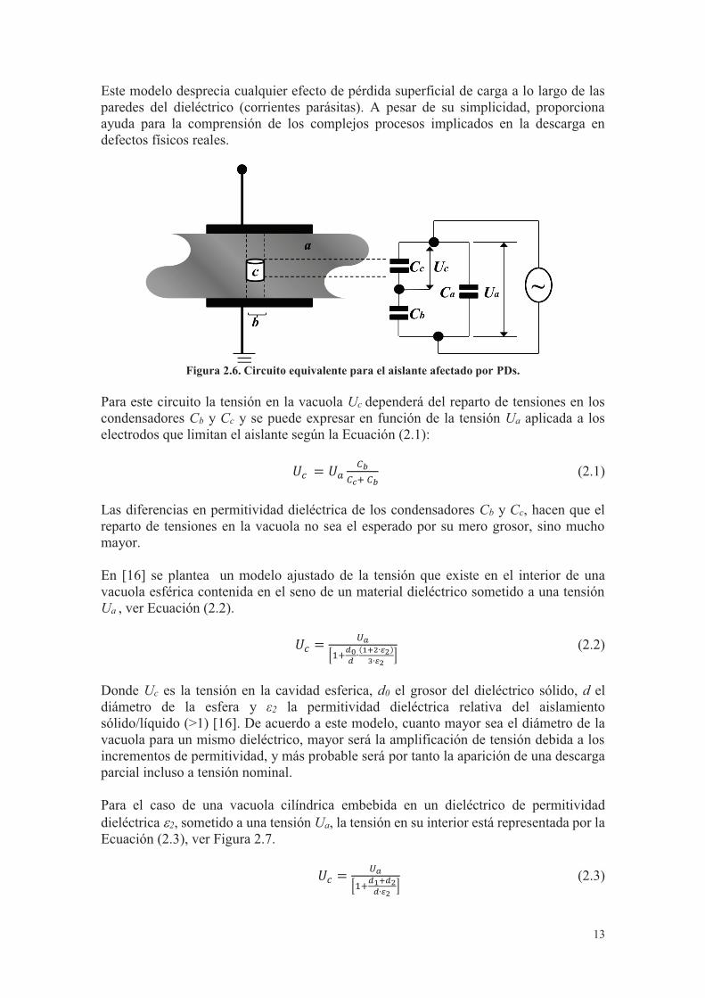
Otra característica importante de este tipo de PDs, es la gran variabilidad estadística de sus magnitudes detectadas (ver Figura 2.4(b)), lo que se debe al fenómeno de la carga espacial anteriormente mencionado y al cambio físico-químico constante en las paredes de las vacuolas. No obstante, son mucho más probables las descargas de menor magnitud. El comportamiento de las PDs internas en corriente alterna, puede ser descrito aproximadamente usando el circuito equivalente propuesto por Whitehead conocido como el modelo “a-b-c” o modelo de los tres condensadores. Este circuito representa el material dieléctrico donde ocurre la descarga mediante la combinación de tres capacidades como se muestra en la Figura 2.6 [15].

Ca: Representa la capacidad del aislamiento sano lejos del entorno de la cavidad.

Cb: Capacidad del aislamiento sano que rodea a la cavidad.

Cc: Es la capacidad equivalente de la vacuola.

14

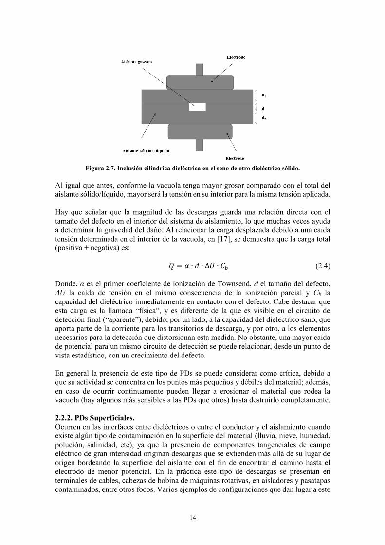
Figura 2.7. Inclusión cilíndrica dieléctrica en el seno de otro dieléctrico sólido.

Al igual que antes, conforme la vacuola tenga mayor grosor comparado con el total del aislante sólido/líquido, mayor será la tensión en su interior para la misma tensión aplicada. Hay que señalar que la magnitud de las descargas guarda una relación directa con el tamaño del defecto en el interior del sistema de aislamiento, lo que muchas veces ayuda a determinar la gravedad del daño. Al relacionar la carga desplazada debido a una caída tensión determinada en el interior de la vacuola, en [17], se demuestra que la carga total (positiva + negativa) es:

𝑄 = 𝛼 ∙ 𝑑 ∙ ∆𝑈 ∙ 𝐶𝑏 (2.4) Donde, α es el primer coeficiente de ionización de Townsend, d el tamaño del defecto, ΔU la caída de tensión en el mismo consecuencia de la ionización parcial y Cb la capacidad del dieléctrico inmediatamente en contacto con el defecto. Cabe destacar que esta carga es la llamada “física”, y es diferente de la que es visible en el circuito de detección final (“aparente”), debido, por un lado, a la capacidad del dieléctrico sano, que aporta parte de la corriente para los transitorios de descarga, y por otro, a los elementos necesarios para la detección que distorsionan esta medida. No obstante, una mayor caída de potencial para un mismo circuito de detección se puede relacionar, desde un punto de vista estadístico, con un crecimiento del defecto. En general la presencia de este tipo de PDs se puede considerar como crítica, debido a que su actividad se concentra en los puntos más pequeños y débiles del material; además, en caso de ocurrir continuamente pueden llegar a erosionar el material que rodea la vacuola (hay algunos más sensibles a las PDs que otros) hasta destruirlo completamente. 2.2.2. PDs Superficiales. Ocurren en las interfaces entre dieléctricos o entre el conductor y el aislamiento cuando existe algún tipo de contaminación en la superficie del material (lluvia, nieve, humedad, polución, salinidad, etc), ya que la presencia de componentes tangenciales de campo eléctrico de gran intensidad originan descargas que se extienden más allá de su lugar de origen bordeando la superficie del aislante con el fin de encontrar el camino hasta el electrodo de menor potencial. En la práctica este tipo de descargas se presentan en terminales de cables, cabezas de bobina de máquinas rotativas, en aisladores y pasatapas contaminados, entre otros focos. Varios ejemplos de configuraciones que dan lugar a este

18

- Son prácticamente inmunes al ruido eléctrico, si las señales se transmiten por fibra óptica.

- Permiten localizar geométricamente fuentes de PDs a través de medida de retardos de señales en más de 3 sensores.

Entre sus desventajas, cabe señalar:

- Posible acoplamiento de otras señales acústicas del exterior. - La mayoría de sensores piezoeléctricos responden en frecuencias en torno a

150kHz, por lo que es complicado separar fuentes de descarga analizando el espectro de los pulsos y es difícil discriminar dos PDs simultáneas que tengan lugar tras pocos microsegundos.

- Las ondas mecánicas sólo se transmiten bien en aceite, por lo que su aplicación está restringida a transformadores de potencia. Si los defectos se encuentran rodeados de grandes masas de materiales dieléctricos sólidos, su detección se hace imposible.

2.3.3. Técnicas químicas. DGA (“Disolved Gas Analysis”). Se basan en el análisis de la concentración de gases en el aceite mineral del transformador (o cable aislado), lo que permite detectar no solo descargas parciales, sino también sobrecalentamientos y otros fallos sufridos. Durante condiciones normales de funcionamiento, hay generalmente una lenta degradación del aceite mineral, que se puede determinar analizando la concentración de gases presentes en el mismo: acetileno, metano, hidrógeno, dióxido de carbono, etileno y oxígeno en forma de ozono. Sin embargo, cuando hay un fallo eléctrico, los gases se generan a una velocidad mucho más rápida. En los devanados de un transformador, los fallos eléctricos más comunes se deben a las PDs; como éstas generan hidrógeno, mediante la determinación de la presencia de este gas y sus cantidades, se puede concluir si existe o no una actividad de PDs. Esta técnica está restringida a sistemas de aislamiento papel-aceite y no permite cuantificar la actividad de descargas parciales [30], [31]. 2.3.4. Técnicas RF (Radio Frequency). Las PDs generan ondas electromagnéticas radiadas que se propagan lejos del lugar de la descarga. La perturbación originada puede llegar a tener componentes en frecuencia que van desde los 100 kHz hasta varios GHz. La máxima radiación que emite una descarga parcial responde a la tasa de cambio de los pulsos de corriente (su derivada); por lo tanto no permite cuantificar su magnitud en términos de pC (como en las técnicas eléctricas), razón por la que esta técnica aún no está estandarizada. Tampoco es posible identificar la polaridad de los pulsos con este método. Se suelen utilizar antenas que trabajan en el rango VHF (30 - 300 MHz) ó UHF (0.3 - 3 GHz), para detectar las ondas electromagnéticas emitidas. Esta técnica presenta las siguientes ventajas [22], [32], [33]:

- Alta sensibilidad, aunque el sistema puede detectar numerosas fuentes de ruido electromagnético en el medio ambiente (FM, TV, GSM, WiFi, etc).

- Adecuadas para medidas en servicio, pues puede ser una técnica no intrusiva y no requiere contacto galvánico con el equipo bajo estudio.

- Permite localizar geométricamente fuentes de descargas parciales.

19

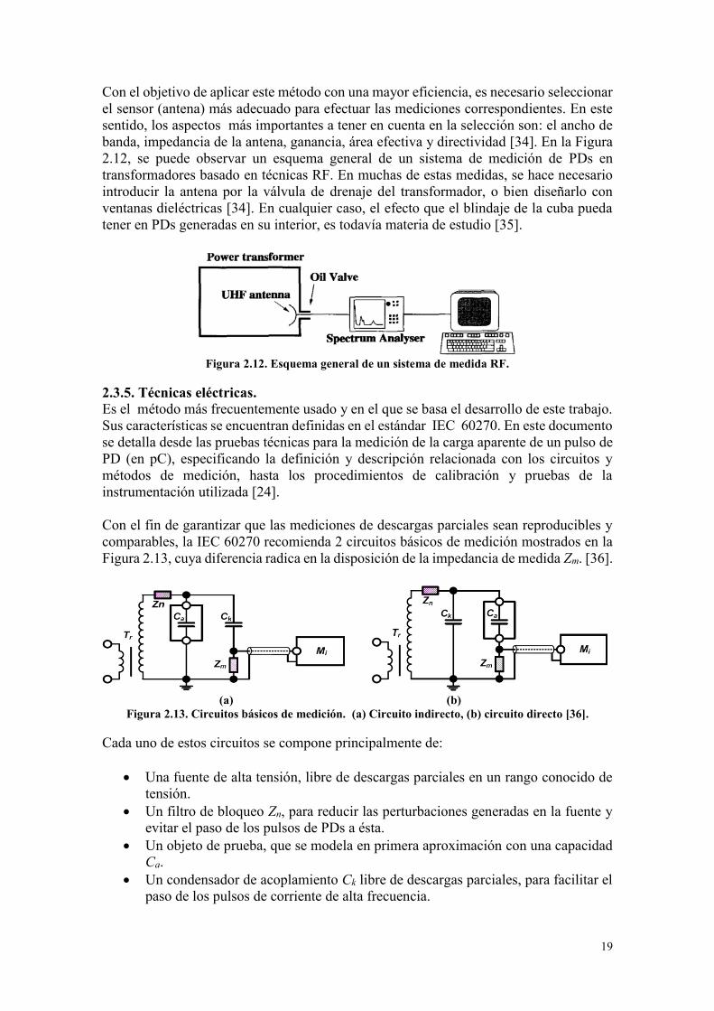
Con el objetivo de aplicar este método con una mayor eficiencia, es necesario seleccionar el sensor (antena) más adecuado para efectuar las mediciones correspondientes. En este sentido, los aspectos más importantes a tener en cuenta en la selección son: el ancho de banda, impedancia de la antena, ganancia, área efectiva y directividad [34]. En la Figura 2.12, se puede observar un esquema general de un sistema de medición de PDs en transformadores basado en técnicas RF. En muchas de estas medidas, se hace necesario introducir la antena por la válvula de drenaje del transformador, o bien diseñarlo con ventanas dieléctricas [34]. En cualquier caso, el efecto que el blindaje de la cuba pueda tener en PDs generadas en su interior, es todavía materia de estudio [35].

Figura 2.12. Esquema general de un sistema de medida RF.

2.3.5. Técnicas eléctricas. Es el método más frecuentemente usado y en el que se basa el desarrollo de este trabajo. Sus características se encuentran definidas en el estándar IEC 60270. En este documento se detalla desde las pruebas técnicas para la medición de la carga aparente de un pulso de PD (en pC), especificando la definición y descripción relacionada con los circuitos y métodos de medición, hasta los procedimientos de calibración y pruebas de la instrumentación utilizada [24]. Con el fin de garantizar que las mediciones de descargas parciales sean reproducibles y comparables, la IEC 60270 recomienda 2 circuitos básicos de medición mostrados en la Figura 2.13, cuya diferencia radica en la disposición de la impedancia de medida Zm. [36].

(a) (b)

Figura 2.13. Circuitos básicos de medición. (a) Circuito indirecto, (b) circuito directo [36].

Cada uno de estos circuitos se compone principalmente de:

Una fuente de alta tensión, libre de descargas parciales en un rango conocido de tensión.

Un filtro de bloqueo Zn, para reducir las perturbaciones generadas en la fuente y evitar el paso de los pulsos de PDs a ésta.

Un objeto de prueba, que se modela en primera aproximación con una capacidad Ca.

Un condensador de acoplamiento Ck libre de descargas parciales, para facilitar el paso de los pulsos de corriente de alta frecuencia.

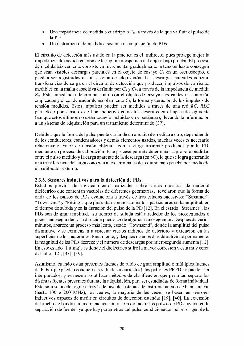
20

Una impedancia de medida o cuadripolo Zm, a través de la que va fluir el pulso de la PD.

Un instrumento de medida o sistema de adquisición de PDs. El circuito de detección más usado en la práctica es el indirecto, pues protege mejor la impedancia de medida en caso de la ruptura inesperada del objeto bajo prueba. El proceso de medida básicamente consiste en incrementar gradualmente la tensión hasta conseguir que sean visibles descargas parciales en el objeto de ensayo Ca en un osciloscopio, o puedan ser registrados en un sistema de adquisición. Las descargas parciales generan transferencias de carga en el circuito de detección que producen impulsos de corriente, medibles en la malla capacitiva definida por Ca y Ck, a través de la impedancia de medida Zm. Esta impedancia determina, junto con el objeto de ensayo, los cables de conexión empleados y el condensador de acoplamiento Ck, la forma y duración de los impulsos de tensión medidos. Estos impulsos pueden ser medidos a través de una red RC, RLC paralelo o por sensores de tipo inductivo como los descritos en el apartado siguiente (aunque estos últimos no están todavía incluidos en el estándar), llevando la información a un sistema de adquisición para un tratamiento determinado [37]. Debido a que la forma del pulso puede variar de un circuito de medida a otro, dependiendo de los conductores, condensadores y demás elementos usados, muchas veces es necesario relacionar el valor de tensión obtenida con la carga aparente producida por la PD, mediante un proceso de calibración. Este proceso permite determinar la proporcionalidad entre el pulso medido y la carga aparente de la descarga (en pC), lo que se logra generando una transferencia de carga conocida a los terminales del equipo bajo prueba por medio de un calibrador externo. 2.3.6. Sensores inductivos para la detección de PDs. Estudios previos de envejecimiento realizados sobre varias muestras de material dieléctrico que contenían vacuolas de diferentes geometrías, revelaron que la forma de onda de los pulsos de PDs evoluciona a través de tres estados sucesivos: “Streamer”, “Townsend” y “Pitting”, que presentan comportamientos particulares en la amplitud, en el tiempo de subida y en la duración del pulso de la PD [12]. En el estado “Streamer”, las PDs son de gran amplitud, su tiempo de subida está alrededor de los picosegundos o pocos nanosegundos y su duración puede ser de algunos nanosegundos. Después de varios minutos, aparece un proceso más lento, estado “Townsend”, donde la amplitud del pulso disminuye y se comienzan a apreciar ciertos indicios de deterioro y oxidación en las superficies de los materiales. Finalmente, y después de unos días de actividad permanente, la magnitud de las PDs decrece y el número de descargas por microsegundo aumenta [12]. En este estado “Pitting”, es donde el dieléctrico sufre la mayor corrosión y está muy cerca del fallo [12], [38], [39]. Asimismo, cuando están presentes fuentes de ruido de gran amplitud o múltiples fuentes de PDs (que pueden conducir a resultados incorrectos), los patrones PRPD no pueden ser interpretados, y es necesario utilizar métodos de clasificación que permitan separar las distintas fuentes presentes durante la adquisición, para ser estudiadas de forma individual. Esto solo se puede lograr a través del uso de sistemas de instrumentación de banda ancha (hasta 100 o 200 MHz), los cuales, la mayoría de las veces, se basan en sensores inductivos capaces de medir en circuitos de detección estándar [19], [40]. La extensión del ancho de banda a altas frecuencias a la hora de medir los pulsos de PDs, ayuda en la separación de fuentes ya que hay parámetros del pulso condicionados por el origen de la

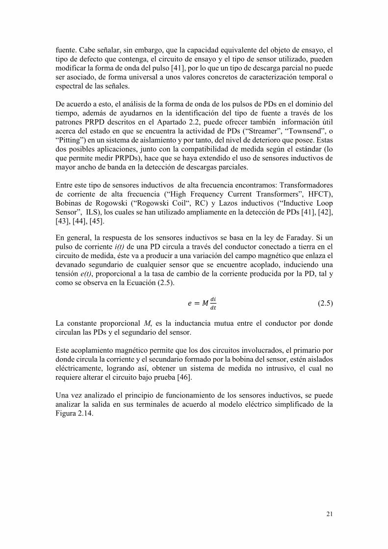
21

fuente. Cabe señalar, sin embargo, que la capacidad equivalente del objeto de ensayo, el tipo de defecto que contenga, el circuito de ensayo y el tipo de sensor utilizado, pueden modificar la forma de onda del pulso [41], por lo que un tipo de descarga parcial no puede ser asociado, de forma universal a unos valores concretos de caracterización temporal o espectral de las señales. De acuerdo a esto, el análisis de la forma de onda de los pulsos de PDs en el dominio del tiempo, además de ayudarnos en la identificación del tipo de fuente a través de los patrones PRPD descritos en el Apartado 2.2, puede ofrecer también información útil acerca del estado en que se encuentra la actividad de PDs (“Streamer”, “Townsend”, o “Pitting”) en un sistema de aislamiento y por tanto, del nivel de deterioro que posee. Estas dos posibles aplicaciones, junto con la compatibilidad de medida según el estándar (lo que permite medir PRPDs), hace que se haya extendido el uso de sensores inductivos de mayor ancho de banda en la detección de descargas parciales. Entre este tipo de sensores inductivos de alta frecuencia encontramos: Transformadores de corriente de alta frecuencia (“High Frequency Current Transformers”, HFCT), Bobinas de Rogowski (“Rogowski Coil“, RC) y Lazos inductivos (“Inductive Loop Sensor”, ILS), los cuales se han utilizado ampliamente en la detección de PDs [41], [42], [43], [44], [45]. En general, la respuesta de los sensores inductivos se basa en la ley de Faraday. Si un pulso de corriente i(t) de una PD circula a través del conductor conectado a tierra en el circuito de medida, éste va a producir a una variación del campo magnético que enlaza el devanado segundario de cualquier sensor que se encuentre acoplado, induciendo una tensión e(t), proporcional a la tasa de cambio de la corriente producida por la PD, tal y como se observa en la Ecuación (2.5).

𝑒 = 𝑀𝑑𝑖

𝑑𝑡 (2.5)

La constante proporcional M, es la inductancia mutua entre el conductor por donde circulan las PDs y el segundario del sensor. Este acoplamiento magnético permite que los dos circuitos involucrados, el primario por donde circula la corriente y el secundario formado por la bobina del sensor, estén aislados eléctricamente, logrando así, obtener un sistema de medida no intrusivo, el cual no requiere alterar el circuito bajo prueba [46]. Una vez analizado el principio de funcionamiento de los sensores inductivos, se puede analizar la salida en sus terminales de acuerdo al modelo eléctrico simplificado de la Figura 2.14.

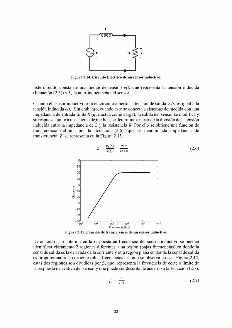
22

Figura 2.14. Circuito Eléctrico de un sensor inductivo.

Este circuito consta de una fuente de tensión e(t) que representa la tensión inducida (Ecuación (2.5)) y L, la auto-inductancia del sensor. Cuando el sensor inductivo está en circuito abierto su tensión de salida vo(t) es igual a la tensión inducida e(t). Sin embargo, cuando éste se conecta a sistemas de medida con una impedancia de entrada finita R (que actúa como carga), la salida del sensor se modifica y su respuesta junto a un sistema de medida, se determina a partir de la división de la tensión inducida entre la impedancia de L y la resistencia R. Por ello se obtiene una función de transferencia definida por la Ecuación (2.6), que se denominada impedancia de transferencia, Z. se representa en la Figura 2.15.

𝑍 =𝑉𝑜(𝑠)

𝐼(𝑠)=

𝑅𝑀𝑠

𝐿𝑠+𝑅 (2.6)

Figura 2.15. Función de transferencia de un sensor inductivo.

De acuerdo a lo anterior, en la respuesta en frecuencia del sensor inductivo se pueden identificar claramente 2 regiones diferentes: una región (bajas frecuencias) en donde la señal de salida es la derivada de la corriente y otra región plana en donde la señal de salida es proporcional a la corriente (altas frecuencias). Como se observa en esta Figura 2.15, estas dos regiones son divididas por fc, que representa la frecuencia de corte o límite de la respuesta derivativa del sensor y que puede ser descrita de acuerdo a la Ecuación (2.7).

𝑓𝑐 =𝑅

2𝜋𝐿 (2.7)

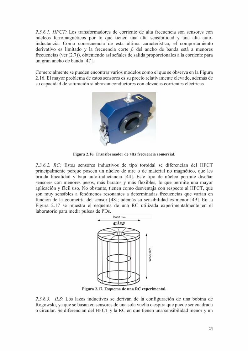
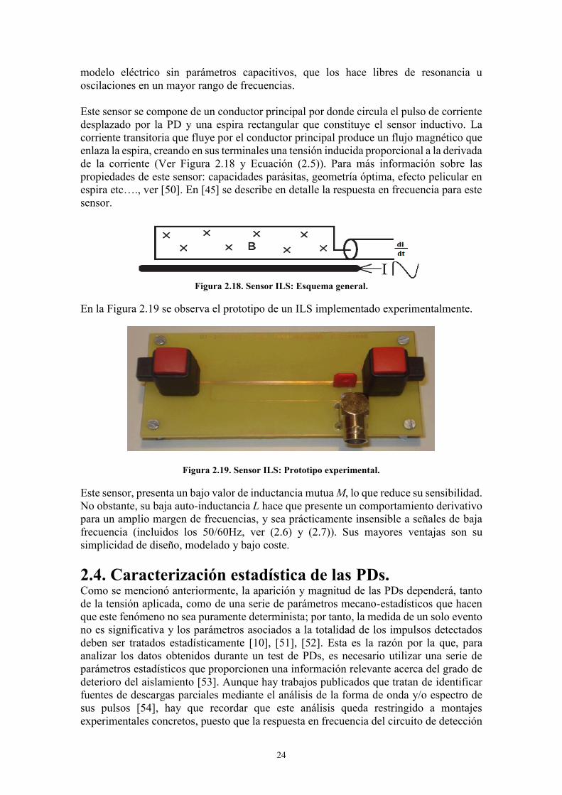
24

modelo eléctrico sin parámetros capacitivos, que los hace libres de resonancia u oscilaciones en un mayor rango de frecuencias. Este sensor se compone de un conductor principal por donde circula el pulso de corriente desplazado por la PD y una espira rectangular que constituye el sensor inductivo. La corriente transitoria que fluye por el conductor principal produce un flujo magnético que enlaza la espira, creando en sus terminales una tensión inducida proporcional a la derivada de la corriente (Ver Figura 2.18 y Ecuación (2.5)). Para más información sobre las propiedades de este sensor: capacidades parásitas, geometría óptima, efecto pelicular en espira etc…., ver [50]. En [45] se describe en detalle la respuesta en frecuencia para este sensor.

Figura 2.18. Sensor ILS: Esquema general.

En la Figura 2.19 se observa el prototipo de un ILS implementado experimentalmente.

Figura 2.19. Sensor ILS: Prototipo experimental. Este sensor, presenta un bajo valor de inductancia mutua M, lo que reduce su sensibilidad. No obstante, su baja auto-inductancia L hace que presente un comportamiento derivativo para un amplio margen de frecuencias, y sea prácticamente insensible a señales de baja frecuencia (incluidos los 50/60Hz, ver (2.6) y (2.7)). Sus mayores ventajas son su simplicidad de diseño, modelado y bajo coste. 2.4. Caracterización estadística de las PDs. Como se mencionó anteriormente, la aparición y magnitud de las PDs dependerá, tanto de la tensión aplicada, como de una serie de parámetros mecano-estadísticos que hacen que este fenómeno no sea puramente determinista; por tanto, la medida de un solo evento no es significativa y los parámetros asociados a la totalidad de los impulsos detectados deben ser tratados estadísticamente [10], [51], [52]. Esta es la razón por la que, para analizar los datos obtenidos durante un test de PDs, es necesario utilizar una serie de parámetros estadísticos que proporcionen una información relevante acerca del grado de deterioro del aislamiento [53]. Aunque hay trabajos publicados que tratan de identificar fuentes de descargas parciales mediante el análisis de la forma de onda y/o espectro de sus pulsos [54], hay que recordar que este análisis queda restringido a montajes experimentales concretos, puesto que la respuesta en frecuencia del circuito de detección

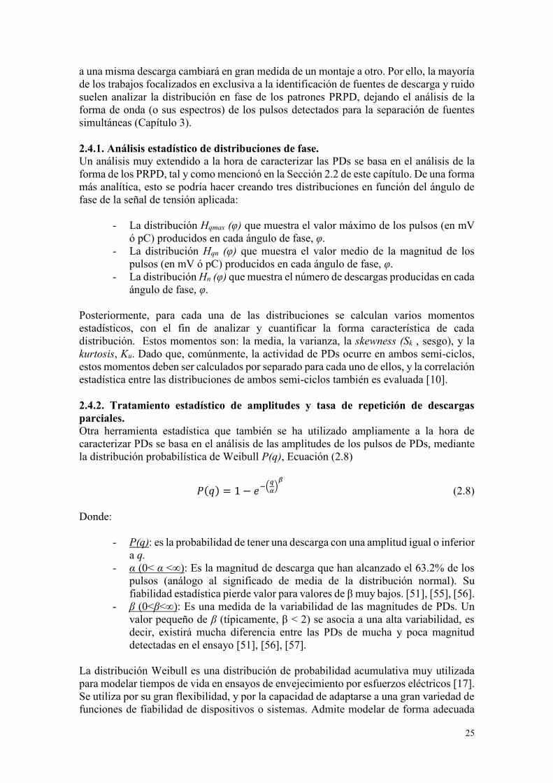
25

a una misma descarga cambiará en gran medida de un montaje a otro. Por ello, la mayoría de los trabajos focalizados en exclusiva a la identificación de fuentes de descarga y ruido suelen analizar la distribución en fase de los patrones PRPD, dejando el análisis de la forma de onda (o sus espectros) de los pulsos detectados para la separación de fuentes simultáneas (Capítulo 3). 2.4.1. Análisis estadístico de distribuciones de fase. Un análisis muy extendido a la hora de caracterizar las PDs se basa en el análisis de la forma de los PRPD, tal y como mencionó en la Sección 2.2 de este capítulo. De una forma más analítica, esto se podría hacer creando tres distribuciones en función del ángulo de fase de la señal de tensión aplicada:

- La distribución Hqmax (φ) que muestra el valor máximo de los pulsos (en mV ó pC) producidos en cada ángulo de fase, φ.

- La distribución Hqn (φ) que muestra el valor medio de la magnitud de los pulsos (en mV ó pC) producidos en cada ángulo de fase, φ.

- La distribución Hn (φ) que muestra el número de descargas producidas en cada ángulo de fase, φ.

Posteriormente, para cada una de las distribuciones se calculan varios momentos estadísticos, con el fin de analizar y cuantificar la forma característica de cada distribución. Estos momentos son: la media, la varianza, la skewness (Sk , sesgo), y la kurtosis, Ku. Dado que, comúnmente, la actividad de PDs ocurre en ambos semi-ciclos, estos momentos deben ser calculados por separado para cada uno de ellos, y la correlación estadística entre las distribuciones de ambos semi-ciclos también es evaluada [10]. 2.4.2. Tratamiento estadístico de amplitudes y tasa de repetición de descargas parciales. Otra herramienta estadística que también se ha utilizado ampliamente a la hora de caracterizar PDs se basa en el análisis de las amplitudes de los pulsos de PDs, mediante la distribución probabilística de Weibull P(q), Ecuación (2.8)

𝑃(𝑞) = 1 − 𝑒−(𝑞

𝛼)

𝛽

(2.8) Donde:

- P(q): es la probabilidad de tener una descarga con una amplitud igual o inferior a q.

- α (0< α <∞): Es la magnitud de descarga que han alcanzado el 63.2% de los pulsos (análogo al significado de media de la distribución normal). Su fiabilidad estadística pierde valor para valores de β muy bajos. [51], [55], [56].

- β (0<β<∞): Es una medida de la variabilidad de las magnitudes de PDs. Un valor pequeño de β (típicamente, β < 2) se asocia a una alta variabilidad, es decir, existirá mucha diferencia entre las PDs de mucha y poca magnitud detectadas en el ensayo [51], [56], [57].

La distribución Weibull es una distribución de probabilidad acumulativa muy utilizada para modelar tiempos de vida en ensayos de envejecimiento por esfuerzos eléctricos [17]. Se utiliza por su gran flexibilidad, y por la capacidad de adaptarse a una gran variedad de funciones de fiabilidad de dispositivos o sistemas. Admite modelar de forma adecuada

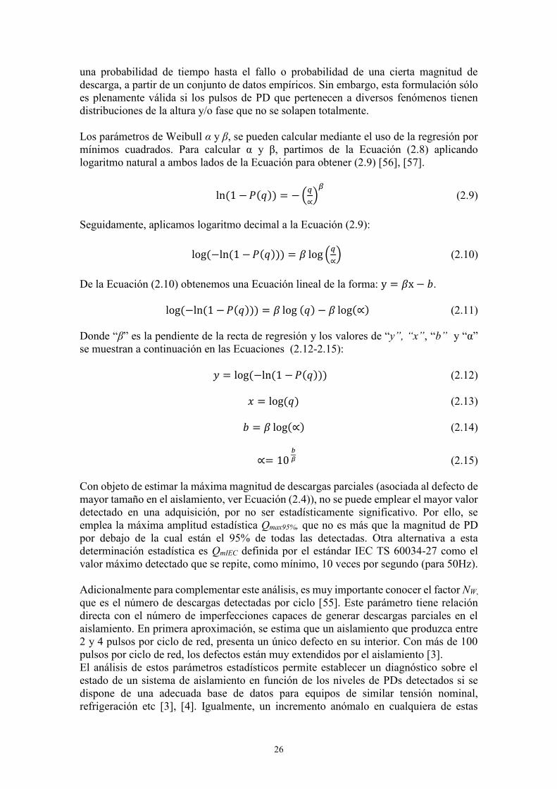
26

una probabilidad de tiempo hasta el fallo o probabilidad de una cierta magnitud de descarga, a partir de un conjunto de datos empíricos. Sin embargo, esta formulación sólo es plenamente válida si los pulsos de PD que pertenecen a diversos fenómenos tienen distribuciones de la altura y/o fase que no se solapen totalmente. Los parámetros de Weibull α y β, se pueden calcular mediante el uso de la regresión por mínimos cuadrados. Para calcular α y β, partimos de la Ecuación (2.8) aplicando logaritmo natural a ambos lados de la Ecuación para obtener (2.9) [56], [57].

ln(1 − 𝑃(𝑞)) = − (𝑞

∝)

𝛽

(2.9) Seguidamente, aplicamos logaritmo decimal a la Ecuación (2.9):

log(−ln(1 − 𝑃(𝑞))) = 𝛽 log (𝑞

∝) (2.10)

De la Ecuación (2.10) obtenemos una Ecuación lineal de la forma: y = 𝛽x − 𝑏.

log(−ln(1 − 𝑃(𝑞))) = 𝛽 log (𝑞) − 𝛽 log(∝) (2.11) Donde “β” es la pendiente de la recta de regresión y los valores de “y”, “x”, “b” y “α” se muestran a continuación en las Ecuaciones (2.12-2.15):

𝑦 = log(−ln(1 − 𝑃(𝑞))) (2.12)

𝑥 = log(𝑞) (2.13)

𝑏 = 𝛽 log(∝) (2.14)

∝= 10 𝑏

𝛽 (2.15)

Con objeto de estimar la máxima magnitud de descargas parciales (asociada al defecto de mayor tamaño en el aislamiento, ver Ecuación (2.4)), no se puede emplear el mayor valor detectado en una adquisición, por no ser estadísticamente significativo. Por ello, se emplea la máxima amplitud estadística Qmax95%, que no es más que la magnitud de PD por debajo de la cual están el 95% de todas las detectadas. Otra alternativa a esta determinación estadística es QmIEC definida por el estándar IEC TS 60034-27 como el valor máximo detectado que se repite, como mínimo, 10 veces por segundo (para 50Hz). Adicionalmente para complementar este análisis, es muy importante conocer el factor NW, que es el número de descargas detectadas por ciclo [55]. Este parámetro tiene relación directa con el número de imperfecciones capaces de generar descargas parciales en el aislamiento. En primera aproximación, se estima que un aislamiento que produzca entre 2 y 4 pulsos por ciclo de red, presenta un único defecto en su interior. Con más de 100 pulsos por ciclo de red, los defectos están muy extendidos por el aislamiento [3]. El análisis de estos parámetros estadísticos permite establecer un diagnóstico sobre el estado de un sistema de aislamiento en función de los niveles de PDs detectados si se dispone de una adecuada base de datos para equipos de similar tensión nominal, refrigeración etc [3], [4]. Igualmente, un incremento anómalo en cualquiera de estas

27

variables estadísticas puede revelar mecanismos de degradación cuya presencia puede ser destructiva para el aislamiento [3], [4], [58]. 2.4.3. Identificación automática de patrones PRPD. En los últimos años, el proceso de identificación se ha intentado realizar de manera automática a través de métodos de inteligencia artificial. Estas aplicaciones lo que buscan en cierta forma es minimizar la intervención humana (que puede realizar una mala interpretación en caso de no tener la experiencia o el conocimiento adecuado a la hora de identificar una determinada fuente) y realizar una identificación basada en parámetros característicos de cada fuente [59], [60]. La efectividad de estos métodos dependerá también, de una etapa previa de separación la cual permitirá evaluar de forma individual la presencia de una u otra fuente. Esto significa que además de las limitaciones propias de cada método, una mala separación entre las diferentes fuentes que puedan estar presentes durante una adquisición (múltiples fuentes de PDs y/o fuentes de ruido), conducirá a obtener resultados erróneos por parte del algoritmo implementado. Esta es la razón de que la separación de fuentes de descargas parciales y ruido se haya convertido en una línea de investigación de gran trascendencia en el ámbito de la gestión de activos eléctricos de alta tensión. Por ello, en el Capítulo 3 se abordará más a fondo esta temática. Dos de los métodos más utilizados en la identificación de fuentes de PDs se describen a continuación: 2.4.3.1. Identificación de fuentes de PDs con algoritmos basados en lógica fuzzy (lógica difusa): La lógica difusa se basa en la observación y en la asignación de valores no concretos a una determinada característica, lo que permite construir una serie de reglas heurísticas que no son ni completamente ciertas ni completamente falsas. De esta forma, los algoritmos basados en lógica fuzzy combinan variables de entrada, definidas en términos de valores difusos, por medio de reglas que producen uno o varios valores de salida. Un ejemplo de aplicación de lógica fuzzy en la identificación de PDs se presenta en [61]. En este trabajo se implementa un algoritmo de clasificación fuzzy para la identificación de fuentes de PDs, que utiliza como elementos de decisión tres tipos diferentes de parámetros [59] propios de las descargas:

Parámetros estándar: tales como DIV, DEV, i (fase de inicio de PDs), e (fase de extinción de PDs), (intervalo o ancho de fases), Smin-Smax (máxima y mínima amplitud detectada), Nw y E (energía media de la PD) entre otros.

Parámetros basados en el análisis de las distribuciones estadísticas Hn(), Hqn() y Hqmax() como m (fase media de la distribución), Sk (Skewness) y Ku (kurtosis), mencionados en el Apartado 2.4.1.

Parámetros basados en el análisis de la amplitud (α y β), tomados de la función probabilística de Weibull descrita en el Apartado 2.4.2.

Tras realizar un estudio sobre el comportamiento de todas estas variables en múltiples experimentos, los autores consideraron que solamente cuatro variables tienen verdadero interés para identificar, mediante las reglas heurísticas adecuadas, las fuentes de descargas y el ruido eléctrico [59]: β, i, m y Sk (para la distribución de amplitudes P(q)).

28

2.4.3.2. Identificación de fuentes de PDs con redes neuronales: Las redes neuronales artificiales (“Neural Networks”, NN) se pueden considerar como un método de aprendizaje y procesamiento que trata de emular el comportamiento del cerebro humano de forma artificial. Se basan en un sistema de interconexión de neuronas que colaboran entre sí para producir un estímulo de salida. Una NN está formada por 3 tipos de neuronas: las neuronas de entrada que reciben las señales desde el entorno, las neuronas de salida que entrega los resultados una vez que se han evaluado y las neuronas ocultas que son las encargadas de realizar el procesamiento. Numerosos trabajos sobre identificación de fuentes de PDs y ruido con redes neuronales se han realizado basándose en el análisis de las distribuciones estadísticas Hn(), Hqn() y Hqmax() (descritas en el Apartado 2.4.1), que se obtienen de la forma de los patrones PRPD asociados a los tres tipos básicos de PDs (corona, internas y superficiales) [62], [63]. Las tipologías más utilizadas para este tipo de aplicaciones han sido: la red de Retro-propagación, la red de auto-organización de Kohonen y la red de aprendizaje de cuantificación vectorial, obteniéndose mejores resultados con la red de Retro-propagación, la cual posee un aprendizaje más rápido y una mejor tasa de reconocimiento [63]. En general, los resultados obtenidos con este tipo de técnicas no han sido del todo buenos, ya que la tasa de éxito en muchos de estos estudios no ha superado el 80% de acierto a la hora de realizar el reconocimiento del tipo de fuente [63]. Entre los principales problemas encontrados al utilizar esta técnica se puede destacar:

La baja tasa de convergencia de la red a la hora identificar correctamente el tipo de fuente.

La dificultad para seleccionar la estructura de la red más adecuada, que en algunos casos varía dependiendo del tipo de fuente que se vaya a detectar.

Los elevados tiempos de entrenamiento y testeo, que varían en función de la estructura de la red que se esté utilizando, y del número de muestras utilizadas para el entrenamiento y testeo de la red.

Debido a esta serie de limitaciones, las NN se han comenzado a combinar con otras técnicas de procesamiento con el fin de minimizar este tipo de falencias, como es el caso del trabajo que se presenta en [64], donde los autores proponen un algoritmo que combina las redes neuronales con un análisis wavelet (ver Capítulo 3), lográndose de esta manera mejorar la convergencia en la identificación del tipo de fuente. Bibliografía.

1. Gill P; “Electrical Power Equipment Maintenance and Testing”; Marcel Dekker; 1998.

2. Wang L., Cavallini A, Montanari G.C, and Testa L; “Evolution of pd patterns in polyethylene insulation cavities under ac voltage”; Dielectrics and Electrical Insulation, IEEE Transactions on, 19(2):533-542, 2012.

3. Stone G, Boutler E.A, Culbert I, Dhirani H; “Electrical Insulation for Rotating Machines: Design, Evaluation, Aging, Testing and Repair”; IEEE Press Series on Power Engineering, Wiley Interscience; 2004.

4. Stone G.C, Warren V; “Effect of Manufacturer, Winding Age and Insulation Type on Stator Winding Partial Discharge Levels”; IEEE Electrical Insulation Magazine; September/October 2004, Vol. 20, No. 5.

29

5. Okabe S, Ueta G, Wada H, and Okubo H; “Partial discharge-induced degradation characteristics of insulating structure constituting oil-immersed power transformers”; Dielectrics and Electrical Insulation, IEEE Transactions on, 17, Vol 5, 1649-1656, 2010.

6. Van Brunt R.J; “Physics and chemistry of partial discharge and corona. Recent advances and future challenges”; Dielectrics and Electrical Insulation, IEEE Transactions on, vol.1, no.5, pp.761,784, Oct 1994.

7. Kuffel E, Zaengl W.S, and Kuffel J; “High Voltage Engineering: Fundamentals”, 2nd ed.; Butterworth-Heinemann; 2000.

8. Khalifa M; “High Voltage Engineering (Theory and Practice)”; 1990. 9. Van Brunt, R.J; “Stochastic properties of partial-discharge phenomena”;

Electrical Insulation, IEEE Transactions, vol.26, no.5, pp.902-948, Oct 1991. 10. Krivda A; “Recognition of Discharges Discrimination and Classification”; Delft

Press; 1995. 11. CIGRE; “Recognition of Discharges”; Electra, 1969. 12. Morshuis P; “Partial Discharge Mechanisms”; Tesis Doctoral, Delft University

Press, The Netherlands, 1993. 13. Kreuger F.H; “Partial Discharge Detection in High-Voltage Equipment”;

Butterworths, London, 1989. 14. Cavallini A, Montanari G. C; “Effect of supply voltage frequency on testing of

insulation system”; Dielectrics and Electrical Insulation, IEEE Transactions on, vol.13, pp. 111- 121, Feb. 2006.

15. Whitehead; “Dielectric Breakdown in solids”; Clarendon Press Oxford 1951. 16. Bartnikas, McMahon; “Engineering Dielectrics, Volume I. Corona Measurements

and Interpretation”; ASTM, Philadelphia, 1979. 17. Dissado L, Fothergill J. C; “Electrical Degradation and Breakdown in Polymers”;

London, IEE Materials and Devices Series, pp 319-339, 1992. 18. Mason J. H; “Enhancing the significance of PD measurements”; Dielectrics and

Electrical Insulation, IEEE Transactions on, vol.2, no.5, pp.876-888, Oct 1995. 19. IEC TS 60034-27-2; “Rotating electrical machines - Part 27-2: On-line partial

discharge measurements on the stator winding insulation of rotating electrical machines”; 2012.

20. Hudon C, Bélec M, Lévesque M; “Study of Slot Partial Discharges in Air-cooled Generators”; Dielectrics and Electrical Insulation, IEEE Transactions on, Vol. 15, No. 6; pp 1675-1690, December 2008.

21. Golinski J, Malewski R, Train D; “Measurements of RIV on Large EHV Apparatus in High Voltage Laboratory”; Power Apparatus and Systems, IEEE Transactions on, vol.PAS-98, pp.817-824, May 1979.

22. Reid A.J, Judd M.D, Fouracre R.A, Stewart B. G, Hepburn D. M; “Simultaneous measurement of partial discharges using IEC60270 and radio-frequency techniques”; Dielectrics and Electrical Insulation, IEEE Transactions on, vol.18, pp.444-455, April 2011.

23. Torres D; “Sistema de Localización de Descargas Parciales en Línea”; Tesis de Maestría, Instituto politécnico nacional, pp. 115, México, 2010.

24. IEC 60270; “High Voltage Test Techniques. Partial Discharge Measurements”; 3a edition, 2000.

25. Norma española UNE 211006. “Ensayos previos a la puesta en servicio de sistemas de cables eléctricos de alta tensión en corriente alterna”. AENOR, 2010.

30

26. Schwarz R, Muhr M; “Modern technologies in optical partial discharge detection”; Electrical Insulation and Dielectric Phenomena, 2007. CEIDP 2007. Annual Report- Conference on, pp.163-166, 14-17 Oct. 2007.

27. Xiaodong Wang, Baoqing Li, Roman H. T, Russo Onofrio L, Chin K, Farmer Kenneth R; “Acousto-optical PD detection for transformers”; Power Delivery, IEEE Transactions on , vol.21, no.3, pp.1068-1073, July 2006.

28. Markalous S, Tenbohlen S, Feser K; “Detection and location of partial discharges in power transformers using acoustic and electromagnetic signals”; Dielectrics and Electrical Insulation, IEEE Transactions on, vol.15, pp.1576-1583, December 2008.

29. Kundu P, Kishore N.K, Sinha A.K; “Identification and Localization of Multi-source Partial Discharges by Acoustic Measurements in Oil-pressboard Insulation System”; Electrical Insulation and Dielectric Phenomena, CEIDP 2008. Annual Report Conference on, pp.383-386, 26-29 Oct. 2008.

30. Ghani A.B.A, Zarim Z.A.A, Majeed J.A, Osman H; “Diagnostic criteria based on the correlation of the measurement of DGA, moisture contents with PD & tan δ in MV oil-filled underground cable”; Dielectric Liquids (ICDL), 2011 IEEE International Conference on, pp.1-4, 26-30 June 2011.

31. “IEEE Guide for the interpretation of gases generated in oil-immersed transformers”, IEEE Std C57.104-2008 (Revision of IEEE Std C57.104-1991), pp. C1-27, 2009.

32. Coenen S, Tenbohlen S, Markalous S.M, Strehl T; “Sensitivity of UHF PD measurements in power transformers”; Dielectrics and Electrical Insulation, IEEE Transactions on, vol.15, pp.1553-1558, December 2008.

33. Muhr M, Schwarz R; “Partial discharge measurement as a Diagnostic Tool for HV-Equipments”; Properties and applications of Dielectric Materials, 2006, 8th International Conference on, pp.195-198, June 2006.

34. Lopez-Roldan J, Tang, T, Gaskin M; “Optimization of a sensor for onsite detection of partial discharges in power transformers by the UHF method”; Dielectrics and Electrical Insulation, IEEE Transactions on, vol.15, pp.1634-1639, December 2008.

35. Robles G, Albarracín R, Martínez-Tarifa J. M; “Shielding effect of power transformers tanks in the ultra-high-frequency detection of partial discharges”; Dielectrics and Electrical Insulation, IEEE Transactions on, Vol. 20, Issue 2, pp: 678-684; April 2013.

36. Lemke E; “Guide for Electrical Partial Discharge measurements in compliance to IEC 60270”; Electra, tomo 241: 61-67, Dic 2008.

37. Ardila-Rey J.A, Martinez-Tarifa J.M, Robles G, Rojas-Moreno M, Albarracin R; “A Partial Discharges acquisition and statistical analysis software”; IEEE, Instrumentation and Measurement Technology Conf. (I2MTC), pp.1670-1675, 2012.

38. Gamez-Garcia M, Bartnikas R, Wertheimer M.R; “Synthesis Reactions Involving XLPE Subjected to partial Discharges”; Electrical Insulation, IEEE Transactions on, vol.EI-22, no.2, pp.199-205, April 1987.

39. Tanaka, T.; “Internal Partial Discharge and Material Degradation”; Electrical Insulation, IEEE Transactions on, vol.EI-21, no.6, pp.899-905, Dec. 1986.

40. IEEE Std 1415-2006; “IEEE Guide for Induction Machinery Maintenance Testing and Failure Analysis”; 2006.

31

41. Cavallini A, Montanari G, Contin A, Pulletti F; “A new approach to the diagnosis of solid insulation systems based on PD signal inference”; IEEE Electrical Insulation Magazine, vol. 19, pp. 22–30, Mar-Apr 2003.

42. Ardila-Rey J.A, Martínez-Tarifa J.M, Robles G, Rojas-Moreno M.V; “Partial Discharge and Noise Separation by Means of Spectral-power Clustering Techniques”; Dielectrics and Electrical Insulation, IEEE Transactions on, Vol. 20, Issue 4, pp: 1436-1443, August 2013.

43. Argüeso M, Robles G, Sanz J; “Implementation of a rogowski coil for the measurement of partial discharges”; Review of Scientic Instruments, Vol, 76 pp. 65107-65107, May 2005.

44. Robles G, Martínez J. M, Sanz J, Tellini B, Zappacosta C, Rojas M; “Designing and tuning an air-cored current transformer for partial discharges pulses measurements”; IEEE Instrumentation and Measurement Technology Conference; Vancouver (Canada); 2008.

45. Rojas-Moreno M. V, Robles G, Tellini B, Zappacosta V, Martínez-Tarifa J. M, Sanz-Feito J; “Study of an Inductive Sensor for Measuring High Frequency Current Pulses”; Instrumentation and Measurements, IEEE Transactions on, Vol 60, nº5, pp 1893-1900, 2011.

46. Nigim K. “Electrical Transformer Testing Handbook”; vol. 4. The Electricity Forum, Ontario, 2007.

47. Gottlieb I; “Practical Transformer Handbook”; Newness, Oxford, 1998. 48. Dubickas V, Edin Hans; "High-Frequency Model of the Rogowski Coil With a

Small Number of Turns"; Instrumentation and Measurement, IEEE Transactions on , vol.56, no.6, pp.2284-2288, Dec. 2007.

49. Ward D, Exon J; “Using Rogowski coils for transient current measurements”; Engineering Science and Education Journal, Vol. 2, pp.105-113, 1993.

50. Robles G, Martínez J. M, Rojas M, Sanz J; “Inductive Sensor for Measuring High Frequency Partial Discharges within Electrical Insulation”; Instrumentation and Measurements, IEEE Transactions on, nº11, 58, pp 3907-39013, Nov 2009.

51. Stone G.C; “The statistics of aging models and practical reality”; Electrical Insulation, IEEE Transactions on, vol.28, pp.716-728, Oct 1993.

52. Lapp A, Kranz H.-G; “The use of the CIGRE data format for PD diagnosis applications”; Dielectrics and Electrical Insulation, IEEE Transactions on, vol.7, pp.102-112, Feb 2000.

53. Contin A, Montanari G.C, Ferraro C; “PD source recognition by Weibull processing of pulse height distributions”; Dielectrics and Electrical Insulation, IEEE Transactions on, vol.7, no.1, pp.48-58, Feb 2000.

54. Ambikairajah, R.; Bao Toan Phung; Ravishankar, J.; Blackburn, T., "Spectral features for the classification of partial discharge signals from selected insulation defect models," Science, Measurement & Technology, IET , vol.7, no.2, pp.104,111, March 2013

55. Cacciari M, Contin A, Rabach G, Montanari G.C, “An approach to partial-discharge investigation by height-distribution analysis”; Science, Measurement and Technology, IEE Proceedings, vol.142, pp.102-108, Jan 1995.

56. Contin A, Contessotto G, Montanari G.C, Cacciari M; “Comparing different stochastic models for the identification and separation of concurrent partial discharge phenomena”; Dielectric Materials, Measurements and Applications,. Eighth International Conference on (IEE Conf. Publ. No. 473), pp.374-379, 2000.

32

57. Cacciari M, Contin A, Montanari G.C; “Use of a mixed-Weibull distribution for the identification of PD phenomena”; Dielectrics and Electrical Insulation, IEEE Transactions on, vol.2, pp.1166-1179, Dec 1995.

58. Tozzi M, Cavallini A, Montanari G.C; “Monitoring Off-line and On-line PD under Impulsive Voltage on Induction Motors – Part 2: Testing”; IEEE Electrical Insulation Magazine, January/February 2011, Vol. 27, No. 1, pp 14-21.

59. Cavallini A, Conti M, Contin A, Montanari G.C; “Advanced PD inference in on-field measurements. II. Identification of defects in solid insulation systems”; Dielectrics and Electrical Insulation, IEEE Transactions on, vol.10, no.3, pp.528-538, June 2003.

60. Sahoo N, Salama M, Bartnikas R; “Trends in partial discharge pattern classification: a survey”; Dielectrics and Electrical Insulation, IEEE Transactions on, Vol. 12(2): 248-264, 2005.

61. Cavallini A, Montanari G.C, Puletti, F, Contin A; “A new methodology for the identification of PD in electrical apparatus: properties and applications”; Dielectrics and Electrical Insulation, IEEE Transactions on, vol.12, pp. 203-215, April 2005.

62. Gulski, E; Krivda A; “Neural networks as a tool for recognition of partial discharges”; Electrical Insulation, IEEE Transactions on, vol.28, no.6, pp.984-1001, Dec 1993.

63. Tao Hong, Fang M. T C; “Detection and classification of partial discharge using a feature decomposition-based modular neural network"; Instrumentation and Measurement, IEEE Transactions on, vol.50, no.5, pp.1349-1354, Oct 2001.

64. Dian-chun Zheng, Chun-xi Zhang, Guo-qing Yang, Xue-yong Sun; “An experiment study of partial discharge pattern recognition method based on wavelet neural networks”; Electrical Insulation, 2006 Conference Record of the 2006 IEEE International Symposium on, pp.230-233, 11-14 June 2006.

33

Capítulo 3

Métodos de separación e identificación de fuentes de PDs y ruido en sistemas de

detección Contenidos 3.1. Separación de PDs y ruido en el dominio del tiempo.............................................. 35 3.2. Separación de fuentes de PDs y ruido a través de descomposición Wavelet .......... 36 3.3. Separación de fuentes de descargas parciales y ruido a través de Mapas T-F ....... 39 3.4. Identificación de fuentes de PDs y ruido a través de Máquina de Vectores Soporte (“Support Vector Machine”, SVM) ................................................................................ 42 3.4.1. Método de Kernel ............................................................................................... 45 3.4.2. Identificación de fuentes de PDs con SVM ........................................................ 46 3.4.2.1 Mejora de la sensibilidad de un sistema de monitorización de PDs utilizando SVM ............................................................................................................................ 47 3.4.2.2 Mejora de la sensibilidad de un sistema de monitorización de PDs utilizando SVM ............................................................................................................................ 48 3.4.2.3 Identificación de PDs en GIS (Gas Insulated Substation) utilizando SVM Multi-Clase ................................................................................................................. 49

Bibliografia ..................................................................................................................... 51

En medidas hechas en entornos industriales reales, los pulsos que tienen como origen descargas parciales y ruido eléctrico se adquieren de forma simultanea dando lugar a complejos patrones PRPD (ver Figura 3.1). En algunos casos las señales de ruido pueden llegar a adquirir magnitudes superiores a las de las propias PDs, por lo que la separación elevando el nivel de disparo de los sistemas de adquisición no es una técnica válida. Este problema está cada vez más extendido por la creciente implantación de convertidores electrónicos de potencia en sistemas eléctricos (variadores de frecuencia, fuentes de alimentación conmutadas, rectificadores, inversores, etc), y por la creciente tendencia a implantar sistemas de medición con los equipos eléctricos en servicio (on-line). Además, algunos tipos de descargas como es el caso de las PDs corona, muchas veces no suelen influir en la expectativa de vida en los sistemas de aislamiento. Algo similar ocurre con algunas fuentes de descargas superficiales (por ejemplo aquellas que se originan en aisladores contaminados), que aunque pudieran ser dañinas, una vez identificadas, muchas de ellas pueden ser mitigadas fácilmente.

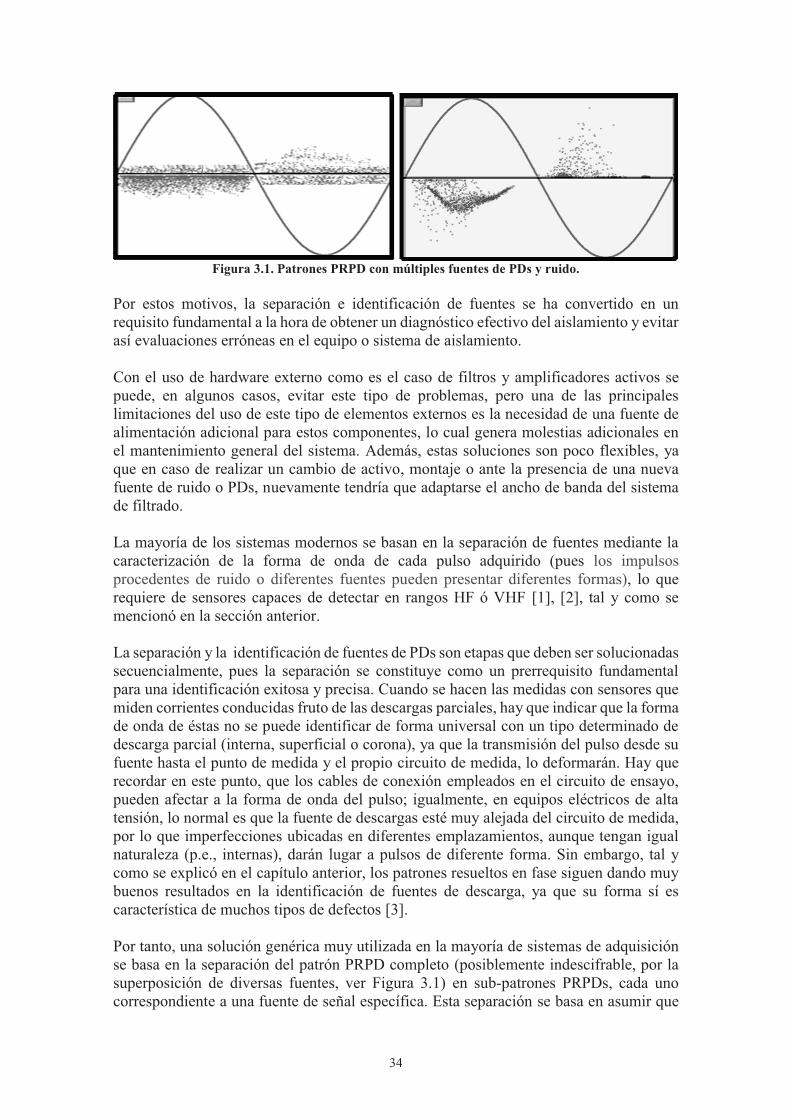
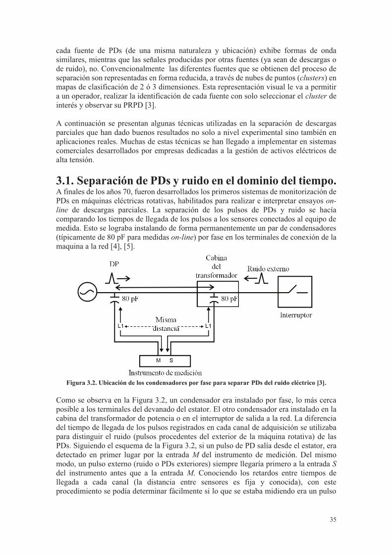
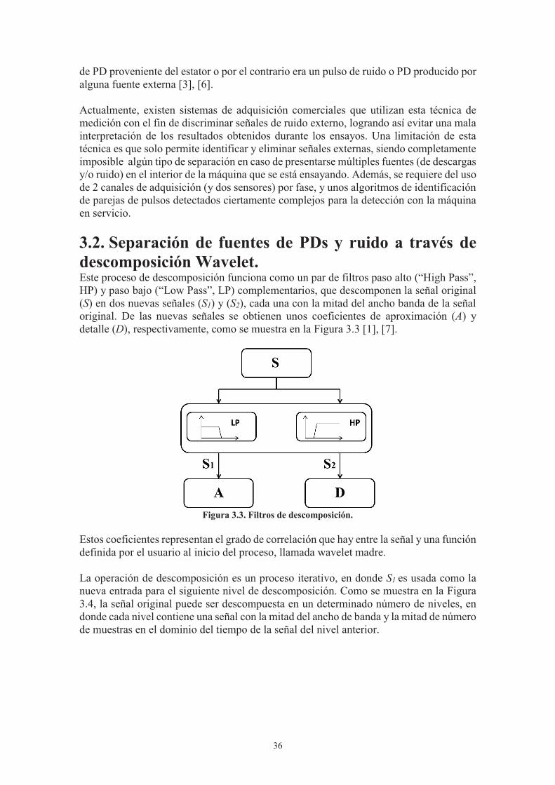
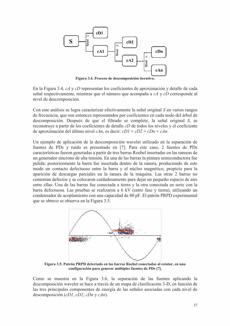
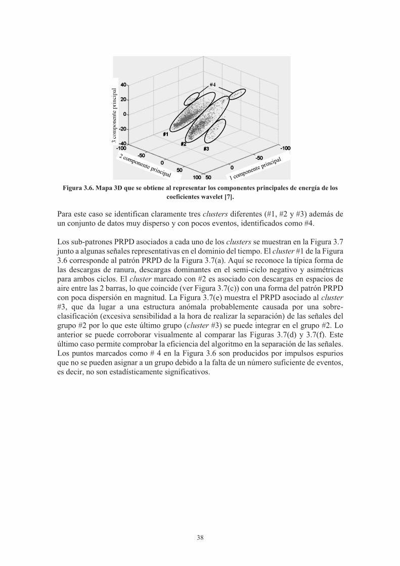
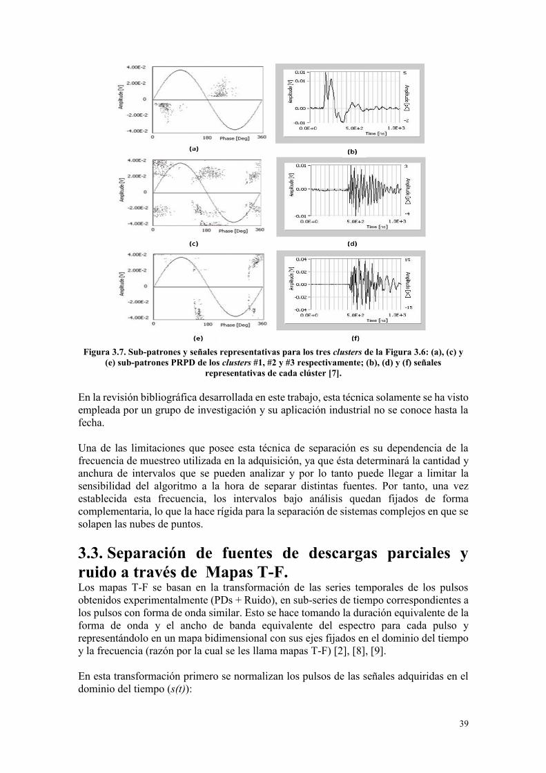
39

Figura 3.7. Sub-patrones y señales representativas para los tres clusters de la Figura 3.6: (a), (c) y

(e) sub-patrones PRPD de los clusters #1, #2 y #3 respectivamente; (b), (d) y (f) señales representativas de cada clúster [7].

En la revisión bibliográfica desarrollada en este trabajo, esta técnica solamente se ha visto empleada por un grupo de investigación y su aplicación industrial no se conoce hasta la fecha. Una de las limitaciones que posee esta técnica de separación es su dependencia de la frecuencia de muestreo utilizada en la adquisición, ya que ésta determinará la cantidad y anchura de intervalos que se pueden analizar y por lo tanto puede llegar a limitar la sensibilidad del algoritmo a la hora de separar distintas fuentes. Por tanto, una vez establecida esta frecuencia, los intervalos bajo análisis quedan fijados de forma complementaria, lo que la hace rígida para la separación de sistemas complejos en que se solapen las nubes de puntos. 3.3. Separación de fuentes de descargas parciales y ruido a través de Mapas T-F. Los mapas T-F se basan en la transformación de las series temporales de los pulsos obtenidos experimentalmente (PDs + Ruido), en sub-series de tiempo correspondientes a los pulsos con forma de onda similar. Esto se hace tomando la duración equivalente de la forma de onda y el ancho de banda equivalente del espectro para cada pulso y representándolo en un mapa bidimensional con sus ejes fijados en el dominio del tiempo y la frecuencia (razón por la cual se les llama mapas T-F) [2], [8], [9]. En esta transformación primero se normalizan los pulsos de las señales adquiridas en el dominio del tiempo (s(t)):

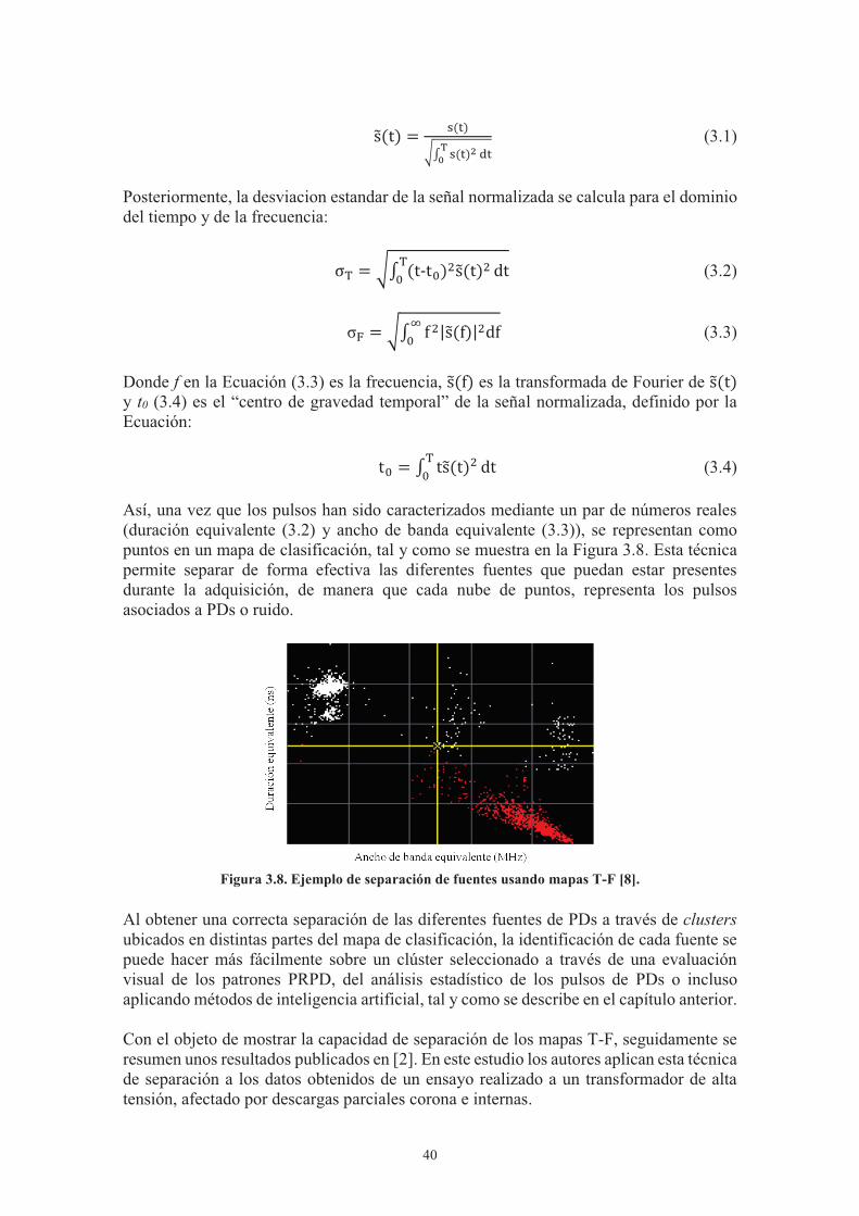
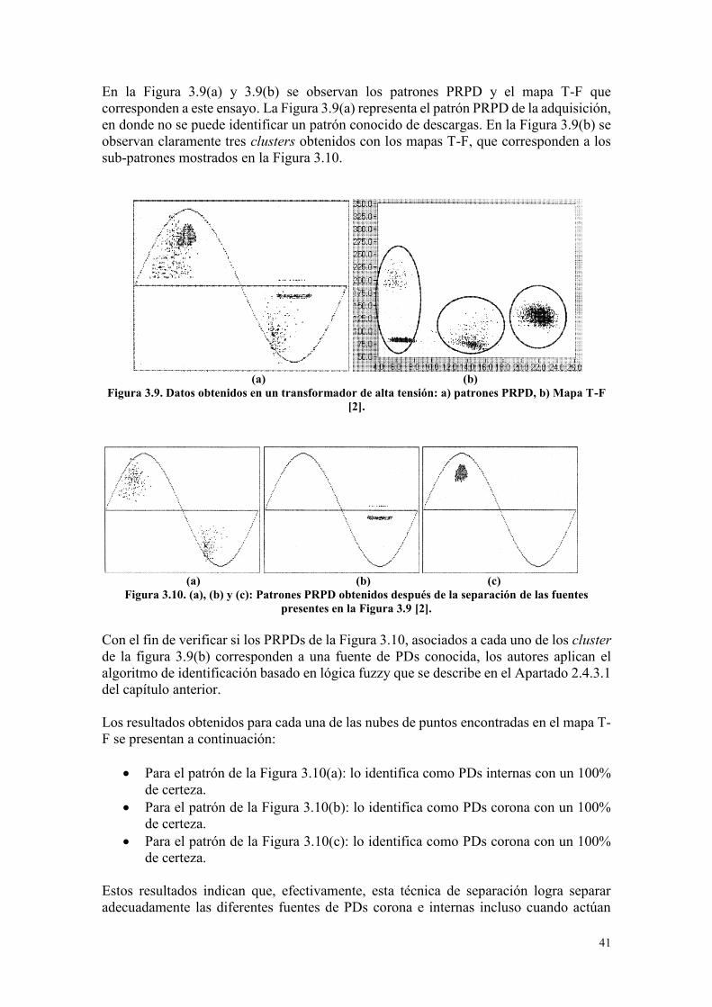
41

En la Figura 3.9(a) y 3.9(b) se observan los patrones PRPD y el mapa T-F que corresponden a este ensayo. La Figura 3.9(a) representa el patrón PRPD de la adquisición, en donde no se puede identificar un patrón conocido de descargas. En la Figura 3.9(b) se observan claramente tres clusters obtenidos con los mapas T-F, que corresponden a los sub-patrones mostrados en la Figura 3.10.

(a) (b) Figura 3.9. Datos obtenidos en un transformador de alta tensión: a) patrones PRPD, b) Mapa T-F

[2].

(a) (b) (c)

Figura 3.10. (a), (b) y (c): Patrones PRPD obtenidos después de la separación de las fuentes presentes en la Figura 3.9 [2].

Con el fin de verificar si los PRPDs de la Figura 3.10, asociados a cada uno de los cluster de la figura 3.9(b) corresponden a una fuente de PDs conocida, los autores aplican el algoritmo de identificación basado en lógica fuzzy que se describe en el Apartado 2.4.3.1 del capítulo anterior. Los resultados obtenidos para cada una de las nubes de puntos encontradas en el mapa T-F se presentan a continuación:

Para el patrón de la Figura 3.10(a): lo identifica como PDs internas con un 100% de certeza.

Para el patrón de la Figura 3.10(b): lo identifica como PDs corona con un 100% de certeza.

Para el patrón de la Figura 3.10(c): lo identifica como PDs corona con un 100% de certeza.

Estos resultados indican que, efectivamente, esta técnica de separación logra separar adecuadamente las diferentes fuentes de PDs corona e internas incluso cuando actúan

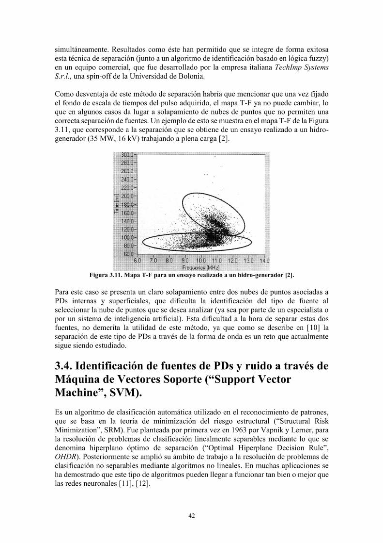
42

simultáneamente. Resultados como éste han permitido que se integre de forma exitosa esta técnica de separación (junto a un algoritmo de identificación basado en lógica fuzzy) en un equipo comercial, que fue desarrollado por la empresa italiana TechImp Systems S.r.l., una spin-off de la Universidad de Bolonia. Como desventaja de este método de separación habría que mencionar que una vez fijado el fondo de escala de tiempos del pulso adquirido, el mapa T-F ya no puede cambiar, lo que en algunos casos da lugar a solapamiento de nubes de puntos que no permiten una correcta separación de fuentes. Un ejemplo de esto se muestra en el mapa T-F de la Figura 3.11, que corresponde a la separación que se obtiene de un ensayo realizado a un hidro-generador (35 MW, 16 kV) trabajando a plena carga [2].

Figura 3.11. Mapa T-F para un ensayo realizado a un hidro-generador [2].

Para este caso se presenta un claro solapamiento entre dos nubes de puntos asociadas a PDs internas y superficiales, que dificulta la identificación del tipo de fuente al seleccionar la nube de puntos que se desea analizar (ya sea por parte de un especialista o por un sistema de inteligencia artificial). Esta dificultad a la hora de separar estas dos fuentes, no demerita la utilidad de este método, ya que como se describe en [10] la separación de este tipo de PDs a través de la forma de onda es un reto que actualmente sigue siendo estudiado. 3.4. Identificación de fuentes de PDs y ruido a través de Máquina de Vectores Soporte (“Support Vector Machine”, SVM). Es un algoritmo de clasificación automática utilizado en el reconocimiento de patrones, que se basa en la teoría de minimización del riesgo estructural (“Structural Risk Minimization”, SRM). Fue planteada por primera vez en 1963 por Vapnik y Lerner, para la resolución de problemas de clasificación linealmente separables mediante lo que se denomina hiperplano óptimo de separación (“Optimal Hiperplane Decision Rule”, OHDR). Posteriormente se amplió su ámbito de trabajo a la resolución de problemas de clasificación no separables mediante algoritmos no lineales. En muchas aplicaciones se ha demostrado que este tipo de algoritmos pueden llegar a funcionar tan bien o mejor que las redes neuronales [11], [12].

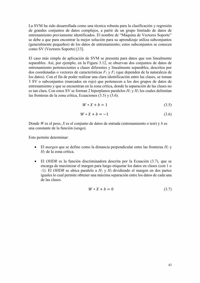
43

La SVM ha sido desarrollada como una técnica robusta para la clasificación y regresión de grandes conjuntos de datos complejos, a partir de un grupo limitado de datos de entrenamiento previamente identificados. El nombre de “Máquina de Vectores Soporte” se debe a que para encontrar la mejor solución para su aprendizaje utiliza subconjuntos (generalmente pequeños) de los datos de entrenamiento; estos subconjuntos se conocen como SV (Vectores Soporte) [13]. El caso más simple de aplicación de SVM se presenta para datos que son linealmente separables. Así, por ejemplo, en la Figura 3.12, se observan dos conjuntos de datos de entrenamiento pertenecientes a clases diferentes y linealmente separables, descritos por dos coordenadas o vectores de características F1 y F2 (que dependen de la naturaleza de los datos). Con el fin de poder realizar una clara identificación entre las clases, se toman 3 SV o subconjuntos (marcados en rojo) que pertenecen a los dos grupos de datos de entrenamiento y que se encuentran en la zona crítica, donde la separación de las clases no es tan clara. Con estos SV se forman 2 hiperplanos paralelos H1 y H2 los cuales delimitan las fronteras de la zona crítica, Ecuaciones (3.5) y (3.6).

𝑊 ∗ 𝑋 + 𝑏 = 1 (3.5)

𝑊 ∗ 𝑋 + 𝑏 = −1 (3.6) Donde W es el peso, X es el conjunto de datos de entrada (entrenamiento o test) y b es una constante de la función (sesgo). Esto permite determinar:

El margen que se define como la distancia perpendicular entre las fronteras H1 y H2 de la zona crítica.

El OHDR es la función discriminadora descrita por la Ecuación (3.7), que se

encarga de maximizar el margen para luego etiquetar los datos en clases (con 1 o -1). El OHDR se ubica paralelo a H1 y H2 dividiendo el margen en dos partes iguales lo cual permite obtener una máxima separación entre los datos de cada una de las clases.

𝑊 ∗ 𝑋 + 𝑏 = 0 (3.7)

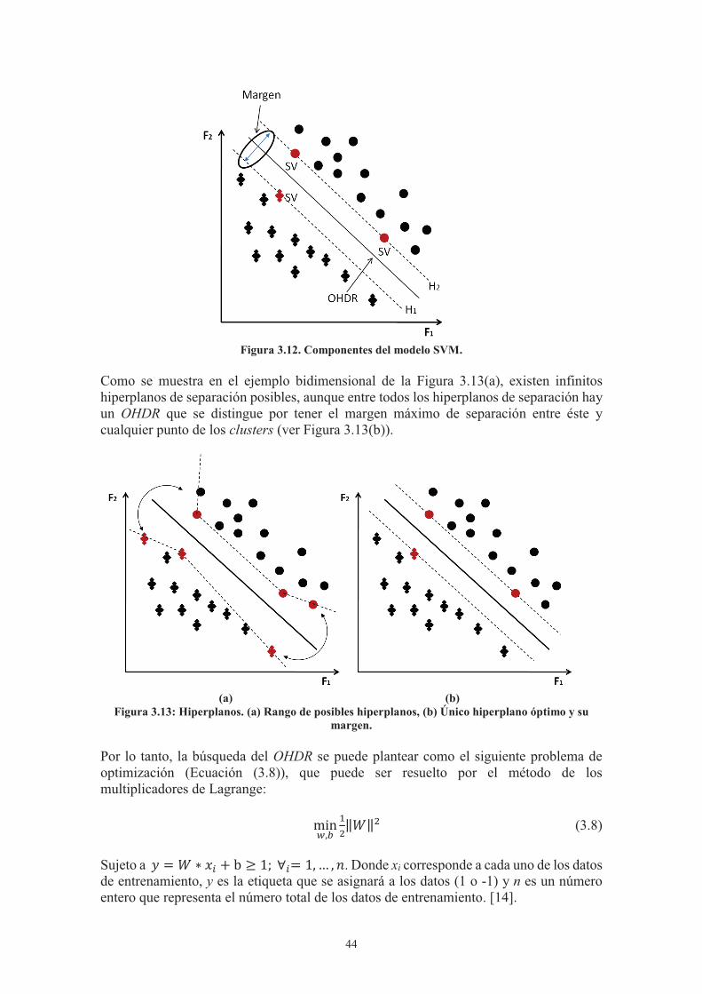
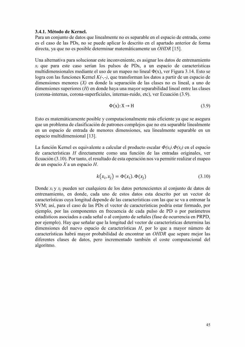
45

3.4.1. Método de Kernel. Para un conjunto de datos que linealmente no es separable en el espacio de entrada, como es el caso de las PDs, no se puede aplicar lo descrito en el apartado anterior de forma directa, ya que no es posible determinar matemáticamente un OHDR [15]. Una alternativa para solucionar este inconveniente, es asignar los datos de entrenamiento xi que para este caso serían los pulsos de PDs, a un espacio de características multidimensionales mediante el uso de un mapeo no lineal Φ(x), ver Figura 3.14. Esto se logra con las funciones Kernel K(-,-), que transforman los datos a partir de un espacio de dimensiones menores (X) en donde la separación de las clases no es lineal, a uno de dimensiones superiores (H) en donde haya una mayor separabilidad lineal entre las clases (corona-internas, corona-superficiales, internas-ruido, etc), ver Ecuación (3.9).

Φ(x): X

→ H (3.9) Esto es matemáticamente posible y computacionalmente más eficiente ya que se asegura que un problema de clasificación de patrones complejos que no era separable linealmente en un espacio de entrada de menores dimensiones, sea linealmente separable en un espacio multidimensional [13]. La función Kernel es equivalente a calcular el producto escalar Φ(xi).Φ(xj) en el espacio de características H directamente como una función de las entradas originales, ver Ecuación (3.10). Por tanto, el resultado de esta operación nos va permitir realizar el mapeo de un espacio X a un espacio H.

𝑘(𝑥𝑖 , 𝑥𝑗) = Φ(𝑥𝑖). Φ(𝑥𝑗) (3.10)

Donde xi y xj pueden ser cualquiera de los datos pertenecientes al conjunto de datos de entrenamiento, en donde, cada uno de estos datos esta descrito por un vector de características cuya longitud depende de las características con las que se va a entrenar la SVM; así, para el caso de las PDs el vector de características podría estar formado, por ejemplo, por las componentes en frecuencia de cada pulso de PD o por parámetros estadísticos asociados a cada señal o al conjunto de señales (fase de ocurrencia en PRPD, por ejemplo). Hay que señalar que la longitud del vector de características determina las dimensiones del nuevo espacio de características H, por lo que a mayor número de características habrá mayor probabilidad de encontrar un OHDR que separe mejor las diferentes clases de datos, pero incrementado también el coste computacional del algoritmo.

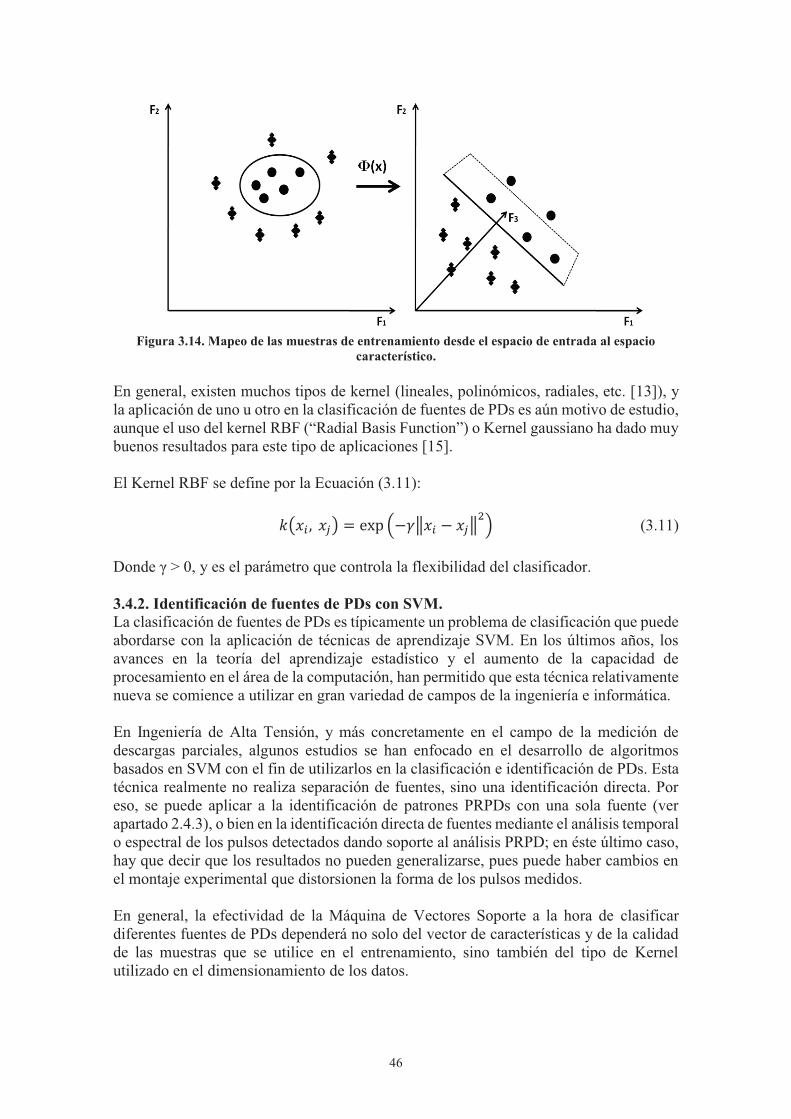
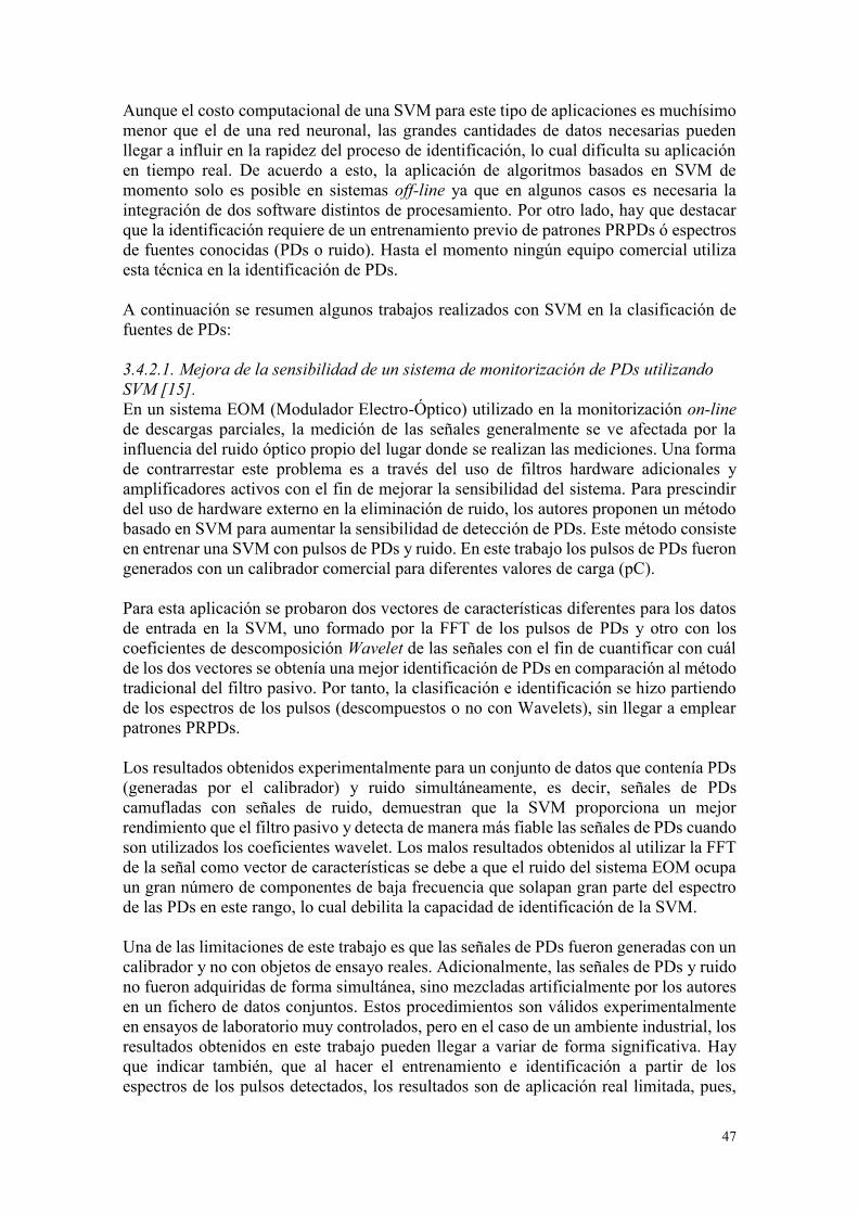
47

Aunque el costo computacional de una SVM para este tipo de aplicaciones es muchísimo menor que el de una red neuronal, las grandes cantidades de datos necesarias pueden llegar a influir en la rapidez del proceso de identificación, lo cual dificulta su aplicación en tiempo real. De acuerdo a esto, la aplicación de algoritmos basados en SVM de momento solo es posible en sistemas off-line ya que en algunos casos es necesaria la integración de dos software distintos de procesamiento. Por otro lado, hay que destacar que la identificación requiere de un entrenamiento previo de patrones PRPDs ó espectros de fuentes conocidas (PDs o ruido). Hasta el momento ningún equipo comercial utiliza esta técnica en la identificación de PDs. A continuación se resumen algunos trabajos realizados con SVM en la clasificación de fuentes de PDs: 3.4.2.1. Mejora de la sensibilidad de un sistema de monitorización de PDs utilizando SVM [15]. En un sistema EOM (Modulador Electro-Óptico) utilizado en la monitorización on-line de descargas parciales, la medición de las señales generalmente se ve afectada por la influencia del ruido óptico propio del lugar donde se realizan las mediciones. Una forma de contrarrestar este problema es a través del uso de filtros hardware adicionales y amplificadores activos con el fin de mejorar la sensibilidad del sistema. Para prescindir del uso de hardware externo en la eliminación de ruido, los autores proponen un método basado en SVM para aumentar la sensibilidad de detección de PDs. Este método consiste en entrenar una SVM con pulsos de PDs y ruido. En este trabajo los pulsos de PDs fueron generados con un calibrador comercial para diferentes valores de carga (pC). Para esta aplicación se probaron dos vectores de características diferentes para los datos de entrada en la SVM, uno formado por la FFT de los pulsos de PDs y otro con los coeficientes de descomposición Wavelet de las señales con el fin de cuantificar con cuál de los dos vectores se obtenía una mejor identificación de PDs en comparación al método tradicional del filtro pasivo. Por tanto, la clasificación e identificación se hizo partiendo de los espectros de los pulsos (descompuestos o no con Wavelets), sin llegar a emplear patrones PRPDs. Los resultados obtenidos experimentalmente para un conjunto de datos que contenía PDs (generadas por el calibrador) y ruido simultáneamente, es decir, señales de PDs camufladas con señales de ruido, demuestran que la SVM proporciona un mejor rendimiento que el filtro pasivo y detecta de manera más fiable las señales de PDs cuando son utilizados los coeficientes wavelet. Los malos resultados obtenidos al utilizar la FFT de la señal como vector de características se debe a que el ruido del sistema EOM ocupa un gran número de componentes de baja frecuencia que solapan gran parte del espectro de las PDs en este rango, lo cual debilita la capacidad de identificación de la SVM. Una de las limitaciones de este trabajo es que las señales de PDs fueron generadas con un calibrador y no con objetos de ensayo reales. Adicionalmente, las señales de PDs y ruido no fueron adquiridas de forma simultánea, sino mezcladas artificialmente por los autores en un fichero de datos conjuntos. Estos procedimientos son válidos experimentalmente en ensayos de laboratorio muy controlados, pero en el caso de un ambiente industrial, los resultados obtenidos en este trabajo pueden llegar a variar de forma significativa. Hay que indicar también, que al hacer el entrenamiento e identificación a partir de los espectros de los pulsos detectados, los resultados son de aplicación real limitada, pues,

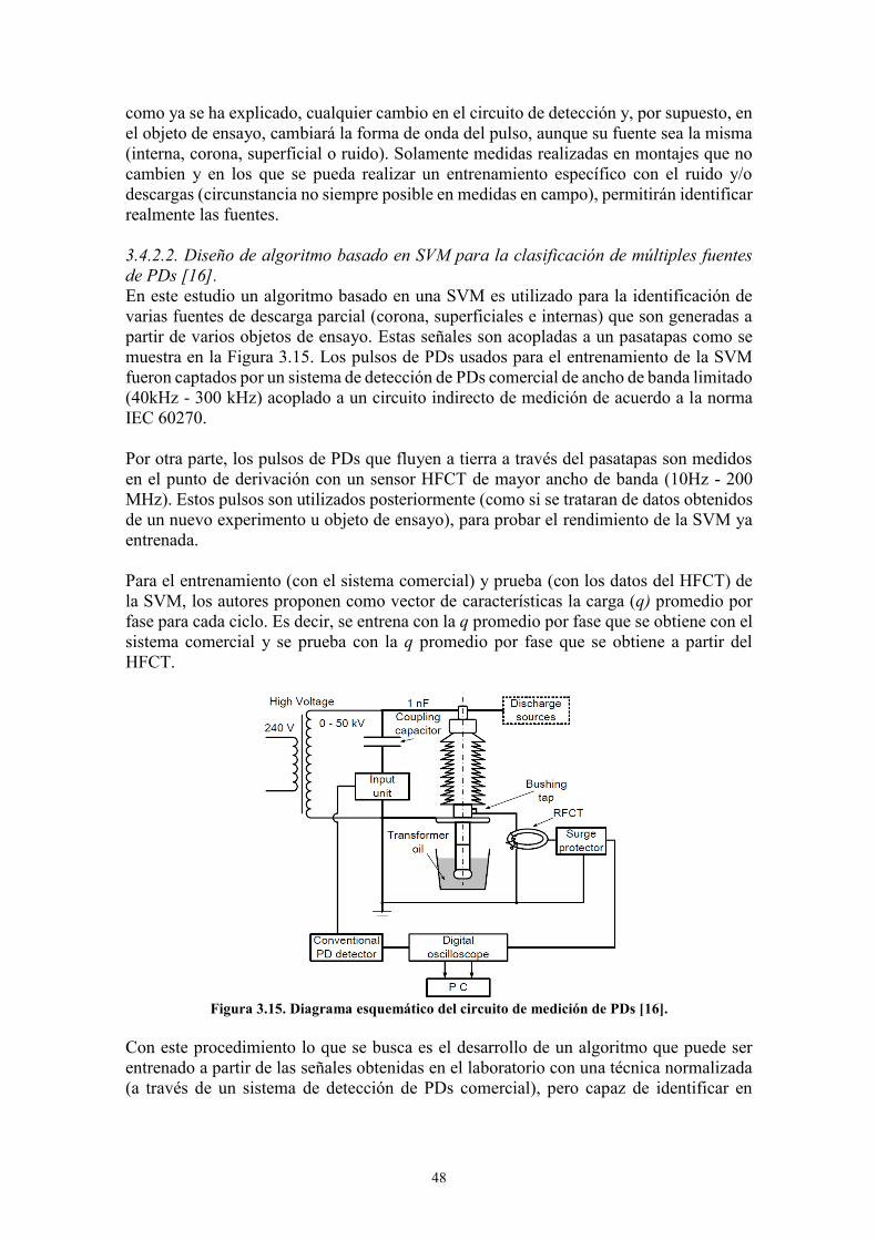
48

como ya se ha explicado, cualquier cambio en el circuito de detección y, por supuesto, en el objeto de ensayo, cambiará la forma de onda del pulso, aunque su fuente sea la misma (interna, corona, superficial o ruido). Solamente medidas realizadas en montajes que no cambien y en los que se pueda realizar un entrenamiento específico con el ruido y/o descargas (circunstancia no siempre posible en medidas en campo), permitirán identificar realmente las fuentes. 3.4.2.2. Diseño de algoritmo basado en SVM para la clasificación de múltiples fuentes de PDs [16]. En este estudio un algoritmo basado en una SVM es utilizado para la identificación de varias fuentes de descarga parcial (corona, superficiales e internas) que son generadas a partir de varios objetos de ensayo. Estas señales son acopladas a un pasatapas como se muestra en la Figura 3.15. Los pulsos de PDs usados para el entrenamiento de la SVM fueron captados por un sistema de detección de PDs comercial de ancho de banda limitado (40kHz - 300 kHz) acoplado a un circuito indirecto de medición de acuerdo a la norma IEC 60270. Por otra parte, los pulsos de PDs que fluyen a tierra a través del pasatapas son medidos en el punto de derivación con un sensor HFCT de mayor ancho de banda (10Hz - 200 MHz). Estos pulsos son utilizados posteriormente (como si se trataran de datos obtenidos de un nuevo experimento u objeto de ensayo), para probar el rendimiento de la SVM ya entrenada.

Para el entrenamiento (con el sistema comercial) y prueba (con los datos del HFCT) de la SVM, los autores proponen como vector de características la carga (q) promedio por fase para cada ciclo. Es decir, se entrena con la q promedio por fase que se obtiene con el sistema comercial y se prueba con la q promedio por fase que se obtiene a partir del HFCT.

Figura 3.15. Diagrama esquemático del circuito de medición de PDs [16].

Con este procedimiento lo que se busca es el desarrollo de un algoritmo que puede ser entrenado a partir de las señales obtenidas en el laboratorio con una técnica normalizada (a través de un sistema de detección de PDs comercial), pero capaz de identificar en

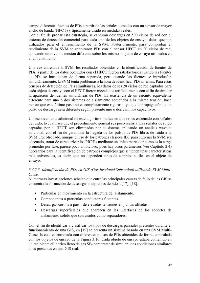
49

campo diferentes fuentes de PDs a partir de las señales tomadas con un sensor de mayor ancho de banda (HFCT) y típicamente usado en medidas reales. Con el fin de probar esta estrategia, se capturan descargas en 500 ciclos de red con el sistema de detección comercial para cada uno de los objetos de ensayo, datos que son utilizados para el entrenamiento de la SVM. Posteriormente, para comprobar el rendimiento de la SVM se capturaron PDs con el sensor HFCT en 20 ciclos de red, aplicando un nivel de tensión diferente sobre los mismos objetos de ensayo utilizados en el entrenamiento. Una vez entrenada la SVM, los resultados obtenidos en la identificación de fuentes de PDs, a partir de los datos obtenidos con el HFCT fueron satisfactorios cuando las fuentes de PDs se introducían de forma separada, pero cuando las fuentes se introducían simultáneamente, la SVM tenía problemas a la hora de identificar PDs internas. Para estas pruebas de detección de PDs simultáneas, los datos de los 20 ciclos de red captados para cada objeto de ensayo con el HFCT fueron mezclados artificialmente con el fin de simular la aparición de fuentes simultáneas de PDs. La existencia de un circuito equivalente diferente para uno o dos sistemas de aislamiento sometidos a la misma tensión, hace pensar que este último paso no es completamente riguroso, ya que la propagación de un pulso de descarga será diferente según presente uno o dos caminos capacitivos. Un inconveniente adicional de este algoritmo radica en que no es entrenado con señales de ruido, lo cual hace que el procedimiento general sea poco realista. Las señales de ruido captadas por el HFCT son eliminadas por el sistema aplicando un análisis wavelet adicional, con el fin de garantizar la llegada de los pulsos de PDs libres de ruido a la SVM. Por otro lado, aunque el uso de los patrones clásicos IEC para entrenar la SVM sea adecuado, tratar de caracterizar los PRPDs mediante un único marcador como es la carga promedio por fase, parece poco ambicioso, pues hay otros parámetros (ver Capítulo 2.4) necesarios para la identificación de patrones complejos que sí tienen unas características más universales, es decir, que no dependen tanto de cambios sutiles en el objeto de ensayo. 3.4.2.3. Identificación de PDs en GIS (Gas Insulated Substation) utilizando SVM Multi-Clase. Numerosas investigaciones señalan que entre las principales causas de fallo de las GIS se encuentra la formación de descargas incipientes debido a [17], [18]:

Partículas en movimiento en la estructura del aislamiento. Componentes o partículas conductoras flotantes. Descargas corona a partir de elevadas tensiones en puntas afiladas. Descargas superficiales que aparecen en las interfaces de los soportes de

aislamiento solido que son usados como separadores. Con el fin de identificar y clasificar los tipos de descargas parciales presentes durante el funcionamiento de una GIS, en [19] se presenta un sistema basado en una SVM Multi-Clase, la cual es entrenada con diferentes pulsos de PDs obtenidos de forma controlada con los objetos de ensayo de la Figura 3.16. Cada objeto de ensayo estaba contenido en un recipiente cilíndrico lleno de gas SF6 para tratar de simular unas condiciones similares a las presentes en una GIS real.

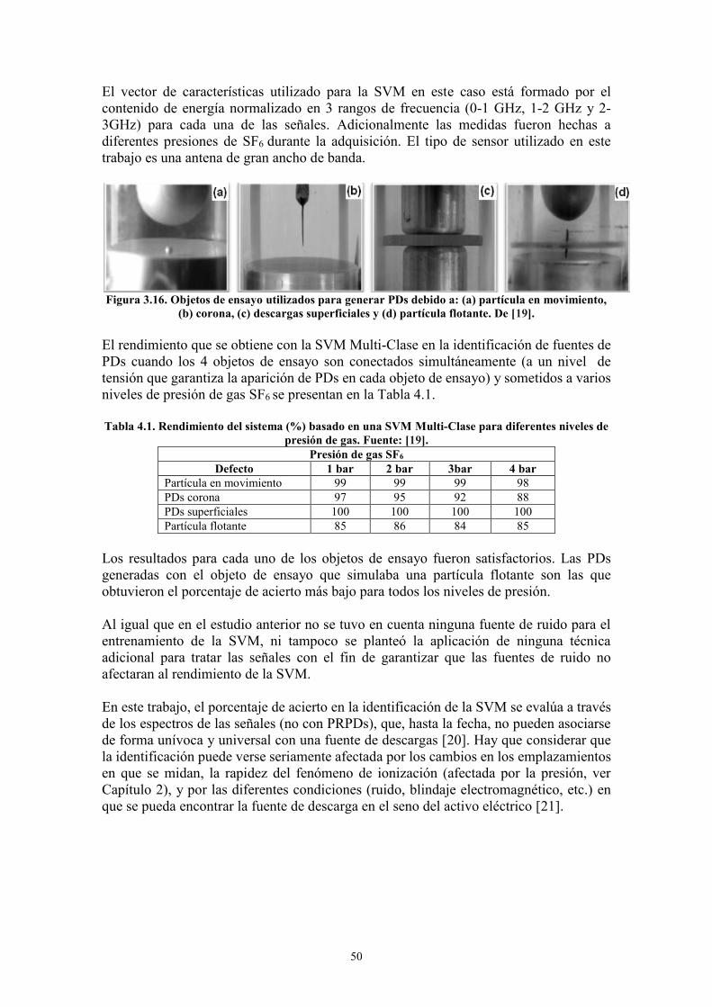
50

El vector de características utilizado para la SVM en este caso está formado por el contenido de energía normalizado en 3 rangos de frecuencia (0-1 GHz, 1-2 GHz y 2-3GHz) para cada una de las señales. Adicionalmente las medidas fueron hechas a diferentes presiones de SF6 durante la adquisición. El tipo de sensor utilizado en este trabajo es una antena de gran ancho de banda.

Figura 3.16. Objetos de ensayo utilizados para generar PDs debido a: (a) partícula en movimiento,

(b) corona, (c) descargas superficiales y (d) partícula flotante. De [19].

El rendimiento que se obtiene con la SVM Multi-Clase en la identificación de fuentes de PDs cuando los 4 objetos de ensayo son conectados simultáneamente (a un nivel de tensión que garantiza la aparición de PDs en cada objeto de ensayo) y sometidos a varios niveles de presión de gas SF6 se presentan en la Tabla 4.1. Tabla 4.1. Rendimiento del sistema (%) basado en una SVM Multi-Clase para diferentes niveles de

presión de gas. Fuente: [19]. Presión de gas SF6

Defecto 1 bar 2 bar 3bar 4 bar Partícula en movimiento 99 99 99 98 PDs corona 97 95 92 88 PDs superficiales 100 100 100 100 Partícula flotante 85 86 84 85

Los resultados para cada uno de los objetos de ensayo fueron satisfactorios. Las PDs generadas con el objeto de ensayo que simulaba una partícula flotante son las que obtuvieron el porcentaje de acierto más bajo para todos los niveles de presión. Al igual que en el estudio anterior no se tuvo en cuenta ninguna fuente de ruido para el entrenamiento de la SVM, ni tampoco se planteó la aplicación de ninguna técnica adicional para tratar las señales con el fin de garantizar que las fuentes de ruido no afectaran al rendimiento de la SVM. En este trabajo, el porcentaje de acierto en la identificación de la SVM se evalúa a través de los espectros de las señales (no con PRPDs), que, hasta la fecha, no pueden asociarse de forma unívoca y universal con una fuente de descargas [20]. Hay que considerar que la identificación puede verse seriamente afectada por los cambios en los emplazamientos en que se midan, la rapidez del fenómeno de ionización (afectada por la presión, ver Capítulo 2), y por las diferentes condiciones (ruido, blindaje electromagnético, etc.) en que se pueda encontrar la fuente de descarga en el seno del activo eléctrico [21].

51

Bibliografía. 1. Sahoo N, Salama M, Bartnikas R; “Trends in partial discharge pattern classification:

a survey”; Dielectrics and Electrical Insulation, IEEE Transactions on, Vol. 12(2): 248-264, 2005.

2. Cavallini A, Montanari, G.C, Puletti F, Contin A; “A new methodology for the identification of PD in electrical apparatus: properties and applications”; Dielectrics and Electrical Insulation, IEEE Transactions on, vol.12, pp. 203- 215, April 2005.

3. IEC/TS 60034-27-2; “Rotating electrical machines- Part 27-2: On-line partial discharge measurements on the stator winding insulation of rotating electrical machines”; Ed. 1.0, 2012.

4. Stone G, Boutler E.A, Culbert I, Dhirani H; “Electrical Insulation for Rotating Machines: Design, Evaluation, Aging, Testing and Repair”; IEEE Press Series on Power Engineering, Wiley Interscience, pp 295-307, 2004.

5. Campbell, S.R.; Stone, G.C.; Sedding, H.G., "Characteristics of partial discharge pulses from operating rotating machines," Electrical Insulation, 1994., Conference Record of the 1994 IEEE International Symposium on , vol., no., pp.229,232, 5-8 Jun 1994.

6. Campbell S. R. et al., “Practical On-Line Partial Discharge Test for Turbine Generators and Motors” IEEE Trans. Energy Conversion, 281–287, June 1994.

7. Hao L, Lewin P.L, Hunter J.A, Swaffield D.J, Contin, A, Walton C, Michel M; “Discrimination of multiple PD sources using wavelet decomposition and principal component analysis”; Dielectrics and Electrical Insulation, IEEE Transactions on, vol.18, pp.1702-1711, October 2011.

8. Cavallini A, Montanari G.C, Contin A, Pulletti F; “A new approach to the diagnosis of solid insulation systems based on PD signal inference”; Electrical Insulation Magazine, IEEE, vol.19, pp.23-30, March-April 2003.

9. Contin A, Cavallini A, Montanari G.C, Pasini, G.; Puletti, F; “Digital detection and fuzzy classification of partial discharge signals”; Dielectrics and Electrical Insulation, IEEE Transactions on , vol.9, no.3, pp.335,348, Jun 2002.

10. Cavallini A, Montanari G.C, Tozzi M, Chen X; “Diagnostic of HVDC systems using partial discharges”; Dielectrics and Electrical Insulation, IEEE Transactions, Vol.18, pp.275-284, 2011.

11. Boser B.E, Guyon I.M, Vapnik, V.N; “A Training Algorithm for Optimal Margin Classifiers”; Proceedings of the fifth Annual Workshop on Computational Learning Theory, pp. 144-152, ACM Press, Nueva York, USA, 1992.

12. Vapnik V.N, Lerner A; “Pattern recognition using generalized portrait method”; Automation and Remote Control, 24(6), pp. 774-780, 1963.

13. Hastie T, Tibshirani R; “Classification by Pairwise Coupling”; The Annals of Statistics, 26(2), pp. 451-471, 1998.

14. Hastie T, Tibshirani R, Friedman J; “The elements of statistical learning”; 2nd ed, Springer series in statistics, 2009.

15. Hao L, Lewin P.L, Dodd S.J; “Improving detection sensitivity for partial discharge monitoring of high voltage equipment”; Mea. Sci. and Tech., Vol. 19. 055707:1-055707:10. ISSN 0957-0233, 2008.

16. Hao L, Lewin P.L; “Partial discharge source discrimination using support vector machine”; IEEE Trans. Dielectr. Electr. Insul, Vol. 17, pp. 189- 197, 2010.

17. IEEE Substations Committee Working Group K4 (GIS diagnostic methods); “Partial discharge testing of gas insulated substations”; IEEE Trans. Power Delivery, Vol. 7, No. 2, pp. 499–506, April 1992.

52

18. CIGRE Working Group D1-11; “Knowledge rules for partial discharge diagnosis in service”; Electra, Vol. 207, No. 8, pp. 63–66, 2003.

19. Umamaheswari R, Sarathi R; “Identification of Partial Discharges in Gas-insulated Switchgear by Ultra-high-frequency Technique and Classification by Adopting Multi-class Support Vector Machines”; Electric Power Components and Systems, 39(14), 1577-1595 2011.

20. Raja K, Devaux F, Lelaidier S; “Recognition of discharge sources using UHF PD signatures”; Electrical Insulation Magazine, IEEE, vol. 18(5), pp. 8-14, 2002.

21. Robles G, Albarracin R, Martinez-Tarifa J.M; “Shielding effect of power transformers tanks in the ultra-high-frequency detection of partial discharges”; Dielectrics and Electrical Insulation, IEEE Transactions on , vol.20, no.2, pp.678,684, April 2013.

53

Capítulo 4

Desarrollo del sistema de adquisición, separación de fuentes y procesamiento de

descargas parciales Contenidos 4.1. Desarrollo del Sistema de adquisición y pre-procesamiento, PD_LINEALT ......... 53 4.1.1. Software del sistema ........................................................................................... 54 4.1.1.1 Adquisición ..................................................................................................... 55 4.1.1.2 Detección de picos .......................................................................................... 56 4.1.1.3 Visualización y almacenamiento .................................................................... 58 4.1.1.3.1 Visualización de patrones PRPD ............................................................... 59 4.1.1.3.2 Forma de onda de un pulso de PD ............................................................. 60 4.1.1.3.3 Espectro de frecuencia de un pulso de PD ................................................. 60 4.1.1.3.4 Mapa PRH-PRL ......................................................................................... 61

4.1.1.4 Pre-procesamiento .......................................................................................... 63 4.1.2. Resultado final del sistema de adquisición ......................................................... 63

4.2. Sistema de separación y procesamiento off-line ..................................................... 65 4.2.1. Ventana “CARGAR DATOS” ........................................................................... 66 4.2.2. Ventana “FILTRAR” .......................................................................................... 67 4.2.3. Ventana “PRPD FILTRADO” ............................................................................ 69

Bibliografía ..................................................................................................................... 70

4.1. Desarrollo del Sistema de adquisición y pre-procesamiento, PD_LINEALT. En la Figura 4.1, se observa el circuito de detección utilizado para el sistema de adquisición de PDs PD_LINEALT, que se presenta en este trabajo. Se basa en la norma IEC 60270 y corresponde al circuito indirecto de detección descrito en el Capítulo 2. Todas las medidas realizadas en los resultados de esta Tesis se basan en el uso de este circuito.

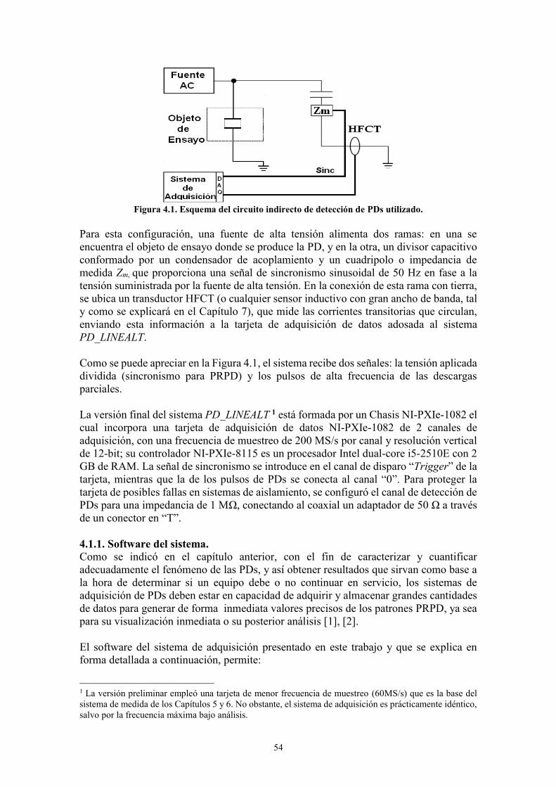
54

Figura 4.1. Esquema del circuito indirecto de detección de PDs utilizado.

Para esta configuración, una fuente de alta tensión alimenta dos ramas: en una se encuentra el objeto de ensayo donde se produce la PD, y en la otra, un divisor capacitivo conformado por un condensador de acoplamiento y un cuadripolo o impedancia de medida Zm, que proporciona una señal de sincronismo sinusoidal de 50 Hz en fase a la tensión suministrada por la fuente de alta tensión. En la conexión de esta rama con tierra, se ubica un transductor HFCT (o cualquier sensor inductivo con gran ancho de banda, tal y como se explicará en el Capítulo 7), que mide las corrientes transitorias que circulan, enviando esta información a la tarjeta de adquisición de datos adosada al sistema PD_LINEALT. Como se puede apreciar en la Figura 4.1, el sistema recibe dos señales: la tensión aplicada dividida (sincronismo para PRPD) y los pulsos de alta frecuencia de las descargas parciales. La versión final del sistema PD_LINEALT 1 está formada por un Chasis NI-PXIe-1082 el cual incorpora una tarjeta de adquisición de datos NI-PXIe-1082 de 2 canales de adquisición, con una frecuencia de muestreo de 200 MS/s por canal y resolución vertical de 12-bit; su controlador NI-PXIe-8115 es un procesador Intel dual-core i5-2510E con 2 GB de RAM. La señal de sincronismo se introduce en el canal de disparo “Trigger” de la tarjeta, mientras que la de los pulsos de PDs se conecta al canal “0”. Para proteger la tarjeta de posibles fallas en sistemas de aislamiento, se configuró el canal de detección de PDs para una impedancia de 1 MΩ, conectando al coaxial un adaptador de 50 Ω a través de un conector en “T”. 4.1.1. Software del sistema. Como se indicó en el capítulo anterior, con el fin de caracterizar y cuantificar adecuadamente el fenómeno de las PDs, y así obtener resultados que sirvan como base a la hora de determinar si un equipo debe o no continuar en servicio, los sistemas de adquisición de PDs deben estar en capacidad de adquirir y almacenar grandes cantidades de datos para generar de forma inmediata valores precisos de los patrones PRPD, ya sea para su visualización inmediata o su posterior análisis [1], [2]. El software del sistema de adquisición presentado en este trabajo y que se explica en forma detallada a continuación, permite:

1 La versión preliminar empleó una tarjeta de menor frecuencia de muestreo (60MS/s) que es la base del sistema de medida de los Capítulos 5 y 6. No obstante, el sistema de adquisición es prácticamente idéntico, salvo por la frecuencia máxima bajo análisis.

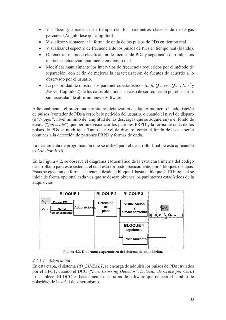
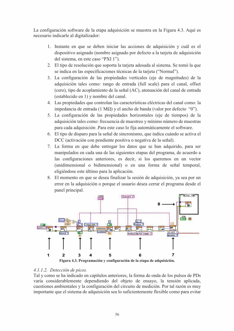
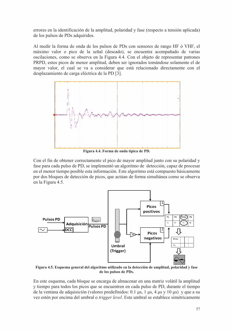
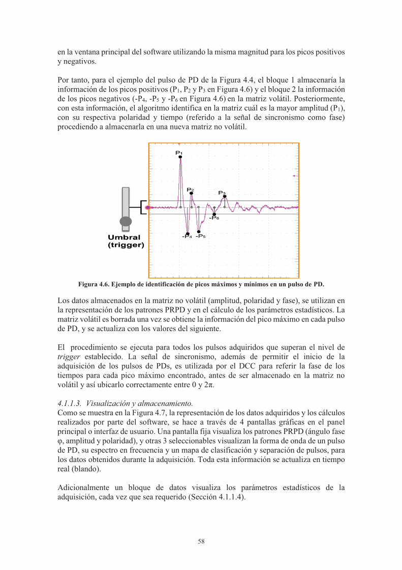
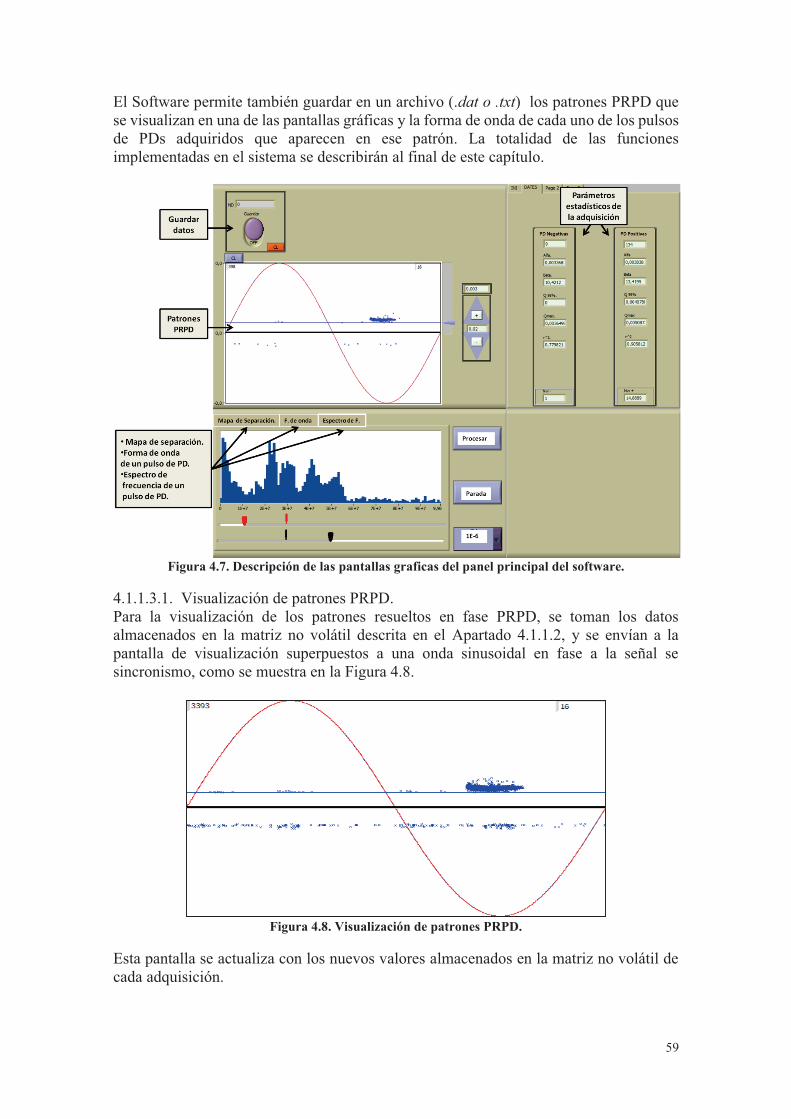
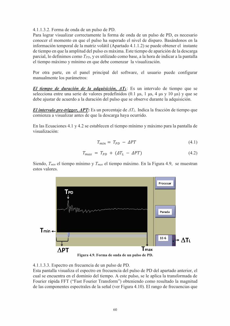
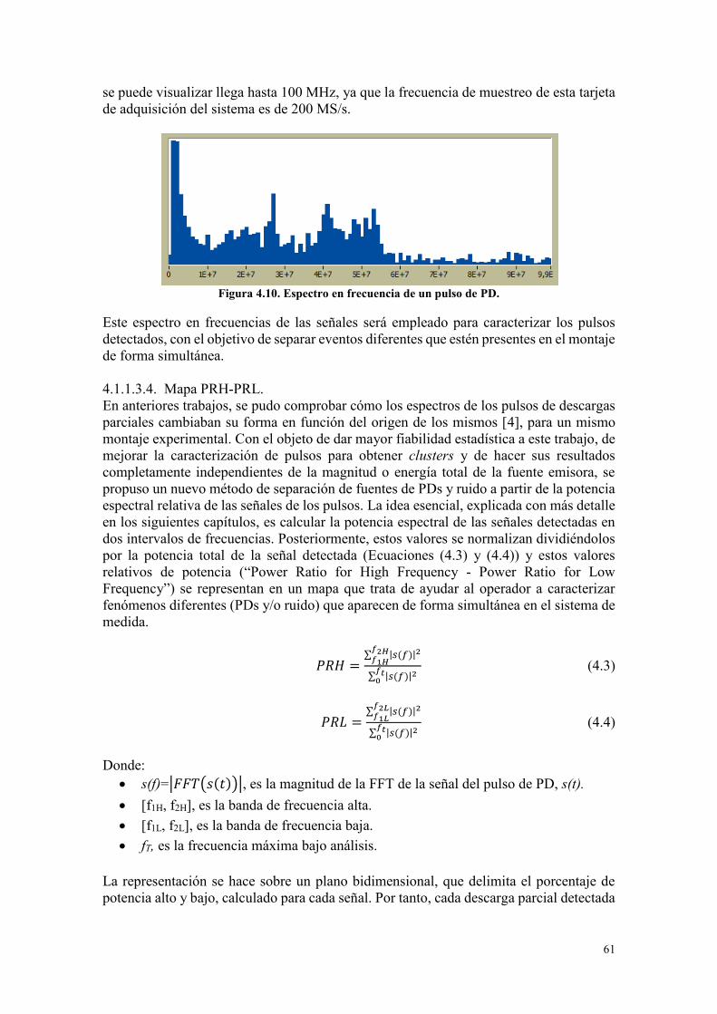
61

se puede visualizar llega hasta 100 MHz, ya que la frecuencia de muestreo de esta tarjeta de adquisición del sistema es de 200 MS/s.

Figura 4.10. Espectro en frecuencia de un pulso de PD.

Este espectro en frecuencias de las señales será empleado para caracterizar los pulsos detectados, con el objetivo de separar eventos diferentes que estén presentes en el montaje de forma simultánea. 4.1.1.3.4. Mapa PRH-PRL. En anteriores trabajos, se pudo comprobar cómo los espectros de los pulsos de descargas parciales cambiaban su forma en función del origen de los mismos [4], para un mismo montaje experimental. Con el objeto de dar mayor fiabilidad estadística a este trabajo, de mejorar la caracterización de pulsos para obtener clusters y de hacer sus resultados completamente independientes de la magnitud o energía total de la fuente emisora, se propuso un nuevo método de separación de fuentes de PDs y ruido a partir de la potencia espectral relativa de las señales de los pulsos. La idea esencial, explicada con más detalle en los siguientes capítulos, es calcular la potencia espectral de las señales detectadas en dos intervalos de frecuencias. Posteriormente, estos valores se normalizan dividiéndolos por la potencia total de la señal detectada (Ecuaciones (4.3) y (4.4)) y estos valores relativos de potencia (“Power Ratio for High Frequency - Power Ratio for Low Frequency”) se representan en un mapa que trata de ayudar al operador a caracterizar fenómenos diferentes (PDs y/o ruido) que aparecen de forma simultánea en el sistema de medida.

𝑃𝑅𝐻 =∑ |𝑠(𝑓)|2𝑓2𝐻

𝑓1𝐻

∑ |𝑠(𝑓)|2𝑓𝑡0

(4.3)

𝑃𝑅𝐿 =∑ |𝑠(𝑓)|2𝑓2𝐿

𝑓1𝐿

∑ |𝑠(𝑓)|2𝑓𝑡0

(4.4)

Donde:

s(f)=|𝐹𝐹𝑇(𝑠(𝑡))|, es la magnitud de la FFT de la señal del pulso de PD, s(t). [f1H, f2H], es la banda de frecuencia alta. [f1L, f2L], es la banda de frecuencia baja. fT, es la frecuencia máxima bajo análisis.

La representación se hace sobre un plano bidimensional, que delimita el porcentaje de potencia alto y bajo, calculado para cada señal. Por tanto, cada descarga parcial detectada

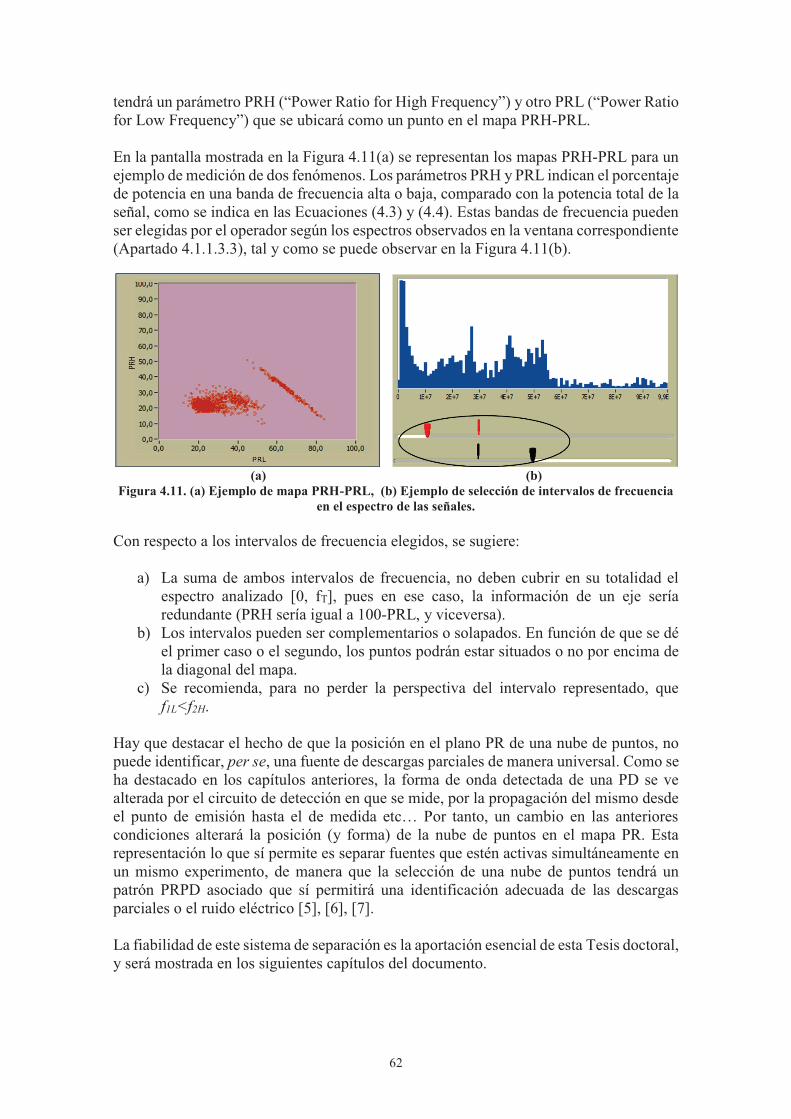
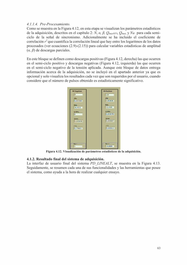
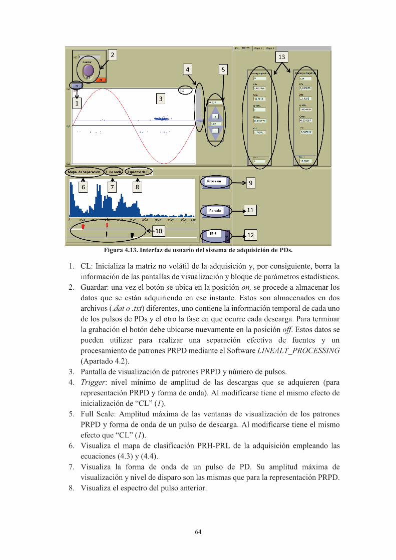
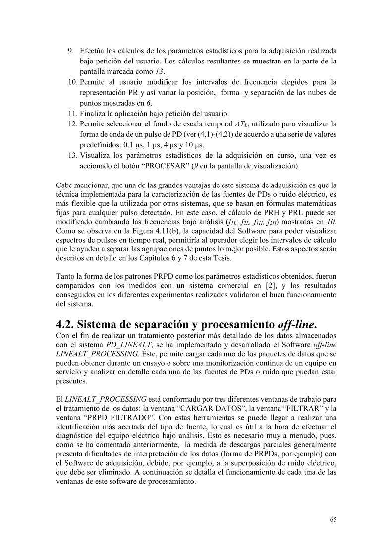
65

9. Efectúa los cálculos de los parámetros estadísticos para la adquisición realizada bajo petición del usuario. Los cálculos resultantes se muestran en la parte de la pantalla marcada como 13.

10. Permite al usuario modificar los intervalos de frecuencia elegidos para la representación PR y así variar la posición, forma y separación de las nubes de puntos mostradas en 6.

11. Finaliza la aplicación bajo petición del usuario. 12. Permite seleccionar el fondo de escala temporal ΔTL, utilizado para visualizar la

forma de onda de un pulso de PD (ver (4.1)-(4.2)) de acuerdo a una serie de valores predefinidos: 0.1 μs, 1 μs, 4 μs y 10 μs.

13. Visualiza los parámetros estadísticos de la adquisición en curso, una vez es accionado el botón “PROCESAR” (9 en la pantalla de visualización).

Cabe mencionar, que una de las grandes ventajas de este sistema de adquisición es que la técnica implementada para la caracterización de las fuentes de PDs o ruido eléctrico, es más flexible que la utilizada por otros sistemas, que se basan en fórmulas matemáticas fijas para cualquier pulso detectado. En este caso, el cálculo de PRH y PRL puede ser modificado cambiando las frecuencias bajo análisis (f1L, f2L, f1H, f2H) mostradas en 10. Como se observa en la Figura 4.11(b), la capacidad del Software para poder visualizar espectros de pulsos en tiempo real, permitiría al operador elegir los intervalos de cálculo que le ayuden a separar las agrupaciones de puntos lo mejor posible. Estos aspectos serán descritos en detalle en los Capítulos 6 y 7 de esta Tesis. Tanto la forma de los patrones PRPD como los parámetros estadísticos obtenidos, fueron comparados con los medidos con un sistema comercial en [2], y los resultados conseguidos en los diferentes experimentos realizados validaron el buen funcionamiento del sistema. 4.2. Sistema de separación y procesamiento off-line. Con el fin de realizar un tratamiento posterior más detallado de los datos almacenados con el sistema PD_LINEALT, se ha implementado y desarrollado el Software off-line LINEALT_PROCESSING. Éste, permite cargar cada uno de los paquetes de datos que se pueden obtener durante un ensayo o sobre una monitorización continua de un equipo en servicio y analizar en detalle cada una de las fuentes de PDs o ruido que puedan estar presentes. El LINEALT_PROCESSING está conformado por tres diferentes ventanas de trabajo para el tratamiento de los datos: la ventana “CARGAR DATOS”, la ventana “FILTRAR” y la ventana “PRPD FILTRADO”. Con estas herramientas se puede llegar a realizar una identificación más acertada del tipo de fuente, lo cual es útil a la hora de efectuar el diagnóstico del equipo eléctrico bajo análisis. Esto es necesario muy a menudo, pues, como se ha comentado anteriormente, la medida de descargas parciales generalmente presenta dificultades de interpretación de los datos (forma de PRPDs, por ejemplo) con el Software de adquisición, debido, por ejemplo, a la superposición de ruido eléctrico, que debe ser eliminado. A continuación se detalla el funcionamiento de cada una de las ventanas de este software de procesamiento.

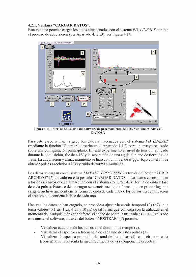
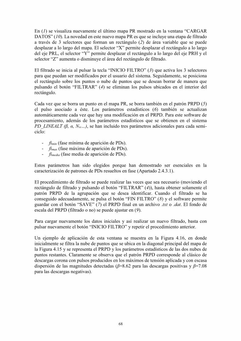
68

En (1) se visualiza nuevamente el último mapa PR mostrado en la ventana “CARGAR DATOS” (10). La novedad en este nuevo mapa PR es que se incluye una etapa de filtrado a través de 3 selectores que forman un rectángulo (2) de área variable que se puede desplazar a lo largo del mapa. El selector “X” permite desplazar el rectángulo a lo largo del eje PRL, el selector “Y” permite desplazar el rectángulo a lo largo del eje PRH y el selector “Z” aumenta o disminuye el área del rectángulo de filtrado. El filtrado se inicia al pulsar la tecla “INICIO FILTRO” (3) que activa los 3 selectores para que puedan ser modificados por el usuario del sistema. Seguidamente, se posiciona el rectángulo sobre los puntos o nube de puntos que se desean borrar de manera que pulsando el botón “FILTRAR” (4) se eliminan los pulsos ubicados en el interior del rectángulo. Cada vez que se borra un punto en el mapa PR, se borra también en el patrón PRPD (5) el pulso asociado a éste. Los parámetros estadísticos (6) también se actualizan automáticamente cada vez que hay una modificación en el PRPD. Para este software de procesamiento, además de los parámetros estadísticos que se obtienen en el sistema PD_LINEALT (β, α, Nw…), se han incluido tres parámetros adicionales para cada semi-ciclo:

- fimin (fase mínima de aparición de PDs). - fimax (fase máxima de aparición de PDs). - fimedia (fase media de aparición de PDs).

Estos parámetros han sido elegidos porque han demostrado ser esenciales en la caracterización de patrones de PDs resueltos en fase (Apartado 2.4.3.1). El procedimiento de filtrado se puede realizar las veces que sea necesario (moviendo el rectángulo de filtrado y pulsando el botón “FILTRAR” (4)), hasta obtener solamente el patrón PRPD de la agrupación que se desea identificar. Cuando el filtrado se ha conseguido adecuadamente, se pulsa el botón “FIN FILTRO” (8) y el software permite guardar con el botón “SAVE” (7) el PRPD final en un archivo .txt o .dat. El fondo de escala del PRPD (filtrado o no) se puede ajustar en (9). Para cargar nuevamente los datos iniciales y así realizar un nuevo filtrado, basta con pulsar nuevamente el botón “INICIO FILTRO” y repetir el procedimiento anterior. Un ejemplo de aplicación de esta ventana se muestra en la Figura 4.16, en donde inicialmente se filtra la nube de puntos que se ubica en la diagonal principal del mapa de la Figura 4.15 y se representa el PRPD y los parámetros estadísticos de las dos nubes de puntos restantes. Claramente se observa que el patrón PRPD corresponde al clásico de descargas corona con pulsos producidos en los máximos de tensión aplicada y con escasa dispersión de las magnitudes detectadas (β=8.62 para las descargas positivas y β=7.08 para las descargas negativas).

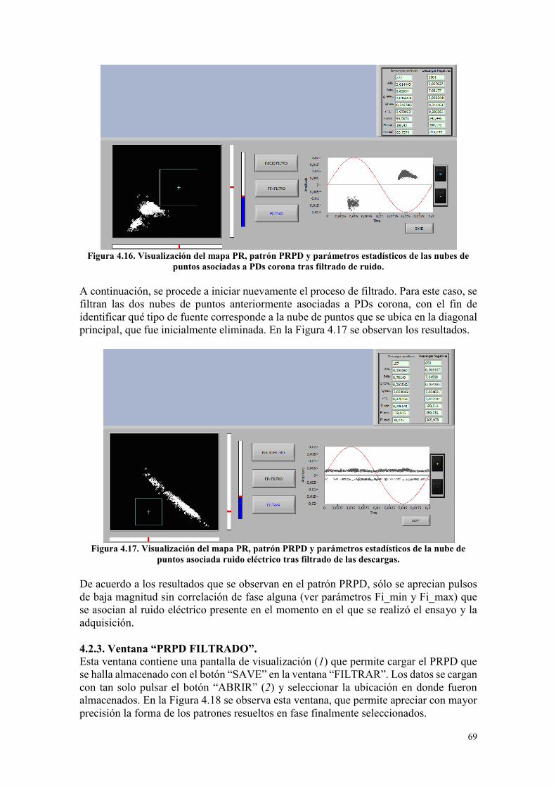
69

Figura 4.16. Visualización del mapa PR, patrón PRPD y parámetros estadísticos de las nubes de

puntos asociadas a PDs corona tras filtrado de ruido. A continuación, se procede a iniciar nuevamente el proceso de filtrado. Para este caso, se filtran las dos nubes de puntos anteriormente asociadas a PDs corona, con el fin de identificar qué tipo de fuente corresponde a la nube de puntos que se ubica en la diagonal principal, que fue inicialmente eliminada. En la Figura 4.17 se observan los resultados.

Figura 4.17. Visualización del mapa PR, patrón PRPD y parámetros estadísticos de la nube de

puntos asociada ruido eléctrico tras filtrado de las descargas. De acuerdo a los resultados que se observan en el patrón PRPD, sólo se aprecian pulsos de baja magnitud sin correlación de fase alguna (ver parámetros Fi_min y Fi_max) que se asocian al ruido eléctrico presente en el momento en el que se realizó el ensayo y la adquisición. 4.2.3. Ventana “PRPD FILTRADO”. Esta ventana contiene una pantalla de visualización (1) que permite cargar el PRPD que se halla almacenado con el botón “SAVE” en la ventana “FILTRAR”. Los datos se cargan con tan solo pulsar el botón “ABRIR” (2) y seleccionar la ubicación en donde fueron almacenados. En la Figura 4.18 se observa esta ventana, que permite apreciar con mayor precisión la forma de los patrones resueltos en fase finalmente seleccionados.

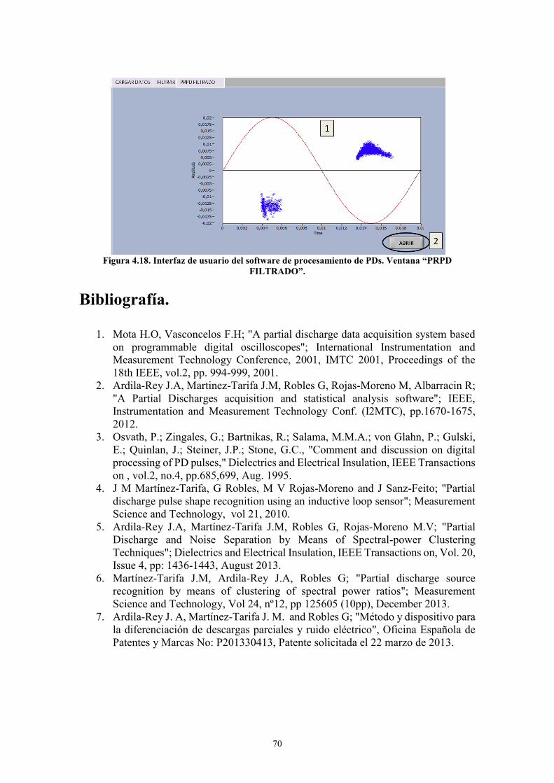
70

Figura 4.18. Interfaz de usuario del software de procesamiento de PDs. Ventana “PRPD

FILTRADO”. Bibliografía.

1. Mota H.O, Vasconcelos F.H; "A partial discharge data acquisition system based on programmable digital oscilloscopes"; International Instrumentation and Measurement Technology Conference, 2001, IMTC 2001, Proceedings of the 18th IEEE, vol.2, pp. 994-999, 2001.

2. Ardila-Rey J.A, Martinez-Tarifa J.M, Robles G, Rojas-Moreno M, Albarracin R; "A Partial Discharges acquisition and statistical analysis software"; IEEE, Instrumentation and Measurement Technology Conf. (I2MTC), pp.1670-1675, 2012.

3. Osvath, P.; Zingales, G.; Bartnikas, R.; Salama, M.M.A.; von Glahn, P.; Gulski, E.; Quinlan, J.; Steiner, J.P.; Stone, G.C., "Comment and discussion on digital processing of PD pulses," Dielectrics and Electrical Insulation, IEEE Transactions on , vol.2, no.4, pp.685,699, Aug. 1995.

4. J M Martínez-Tarifa, G Robles, M V Rojas-Moreno and J Sanz-Feito; "Partial discharge pulse shape recognition using an inductive loop sensor"; Measurement Science and Technology, vol 21, 2010.

5. Ardila-Rey J.A, Martínez-Tarifa J.M, Robles G, Rojas-Moreno M.V; "Partial Discharge and Noise Separation by Means of Spectral-power Clustering Techniques"; Dielectrics and Electrical Insulation, IEEE Transactions on, Vol. 20, Issue 4, pp: 1436-1443, August 2013.

6. Martínez-Tarifa J.M, Ardila-Rey J.A, Robles G; "Partial discharge source recognition by means of clustering of spectral power ratios"; Measurement Science and Technology, Vol 24, nº12, pp 125605 (10pp), December 2013.

7. Ardila-Rey J. A, Martínez-Tarifa J. M. and Robles G; "Método y dispositivo para la diferenciación de descargas parciales y ruido eléctrico", Oficina Española de Patentes y Marcas No: P201330413, Patente solicitada el 22 marzo de 2013.

Chapter 5

Partial Discharge and Noise Separation by Means of Spectral-power Clustering

Techniques

Contents 5.1. Abstract .................................................................................................................... 71 5.2. Introduction ............................................................................................................. 71 5.3. Spectral power analysis and processing technique .................................................. 73 5.4. Experimental setup .................................................................................................. 74 5.5. Design of the partial discharge sources ................................................................... 75 5.5.1. Surface discharges .............................................................................................. 75 5.5.2. Internal discharges .............................................................................................. 75 5.5.3. Corona discharges ............................................................................................... 76

5.6. Experimental measurements for PD sources identification ..................................... 78 5.6.1. Surface discharges: experiment #1 ..................................................................... 78 5.6.2. Internal discharges: experiment #2 ..................................................................... 79 5.6.3. Corona discharges: experiment #3...................................................................... 81

5.7. Summary .................................................................................................................. 82 5.8. Discussion ................................................................................................................ 83 References ...................................................................................................................... 83

5.1. Abstract. Partial Discharges (PDs) are one of the most important classes of ageing processes that occur within electrical insulation. The measurement of PDs is useful in the diagnosis of electrical equipment because PDs activity is related to different ageing mechanisms. Classical Phase-Resolved Partial Discharge (PRPD) patterns are able to identify PD sources when they are related to a clear degradation process and when the noise level is low compared to the amplitudes of the PDs. However, real insulation systems usually exhibit several PD sources and the noise level is high, especially if measurements are performed on-line. High-frequency (HF) sensors and advanced signal processing techniques have been successfully applied to identify these phenomena in real insulation systems. In this paper, spectral power analyses of PD pulses and the spectral power ratios at different frequencies were calculated to classify PD sources and noise by means of a graphical representation in a plane. This technique is a flexible tool for noise identification and will be useful for pulse characterization.

5.2. Introduction. The failure of electrical insulation is one of the most important causes of power equipment outages. Classical causes of faults in power systems are related to mechanical, thermal or

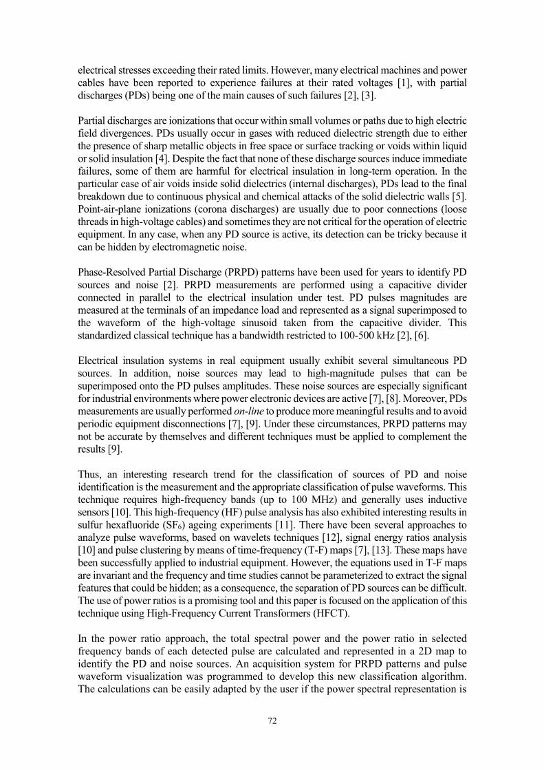
72

electrical stresses exceeding their rated limits. However, many electrical machines and power cables have been reported to experience failures at their rated voltages [1], with partial discharges (PDs) being one of the main causes of such failures [2], [3]. Partial discharges are ionizations that occur within small volumes or paths due to high electric field divergences. PDs usually occur in gases with reduced dielectric strength due to either the presence of sharp metallic objects in free space or surface tracking or voids within liquid or solid insulation [4]. Despite the fact that none of these discharge sources induce immediate failures, some of them are harmful for electrical insulation in long-term operation. In the particular case of air voids inside solid dielectrics (internal discharges), PDs lead to the final breakdown due to continuous physical and chemical attacks of the solid dielectric walls [5]. Point-air-plane ionizations (corona discharges) are usually due to poor connections (loose threads in high-voltage cables) and sometimes they are not critical for the operation of electric equipment. In any case, when any PD source is active, its detection can be tricky because it can be hidden by electromagnetic noise. Phase-Resolved Partial Discharge (PRPD) patterns have been used for years to identify PD sources and noise [2]. PRPD measurements are performed using a capacitive divider connected in parallel to the electrical insulation under test. PD pulses magnitudes are measured at the terminals of an impedance load and represented as a signal superimposed to the waveform of the high-voltage sinusoid taken from the capacitive divider. This standardized classical technique has a bandwidth restricted to 100-500 kHz [2], [6]. Electrical insulation systems in real equipment usually exhibit several simultaneous PD sources. In addition, noise sources may lead to high-magnitude pulses that can be superimposed onto the PD pulses amplitudes. These noise sources are especially significant for industrial environments where power electronic devices are active [7], [8]. Moreover, PDs measurements are usually performed on-line to produce more meaningful results and to avoid periodic equipment disconnections [7], [9]. Under these circumstances, PRPD patterns may not be accurate by themselves and different techniques must be applied to complement the results [9]. Thus, an interesting research trend for the classification of sources of PD and noise identification is the measurement and the appropriate classification of pulse waveforms. This technique requires high-frequency bands (up to 100 MHz) and generally uses inductive sensors [10]. This high-frequency (HF) pulse analysis has also exhibited interesting results in sulfur hexafluoride (SF6) ageing experiments [11]. There have been several approaches to analyze pulse waveforms, based on wavelets techniques [12], signal energy ratios analysis [10] and pulse clustering by means of time-frequency (T-F) maps [7], [13]. These maps have been successfully applied to industrial equipment. However, the equations used in T-F maps are invariant and the frequency and time studies cannot be parameterized to extract the signal features that could be hidden; as a consequence, the separation of PD sources can be difficult. The use of power ratios is a promising tool and this paper is focused on the application of this technique using High-Frequency Current Transformers (HFCT). In the power ratio approach, the total spectral power and the power ratio in selected frequency bands of each detected pulse are calculated and represented in a 2D map to identify the PD and noise sources. An acquisition system for PRPD patterns and pulse waveform visualization was programmed to develop this new classification algorithm. The calculations can be easily adapted by the user if the power spectral representation is

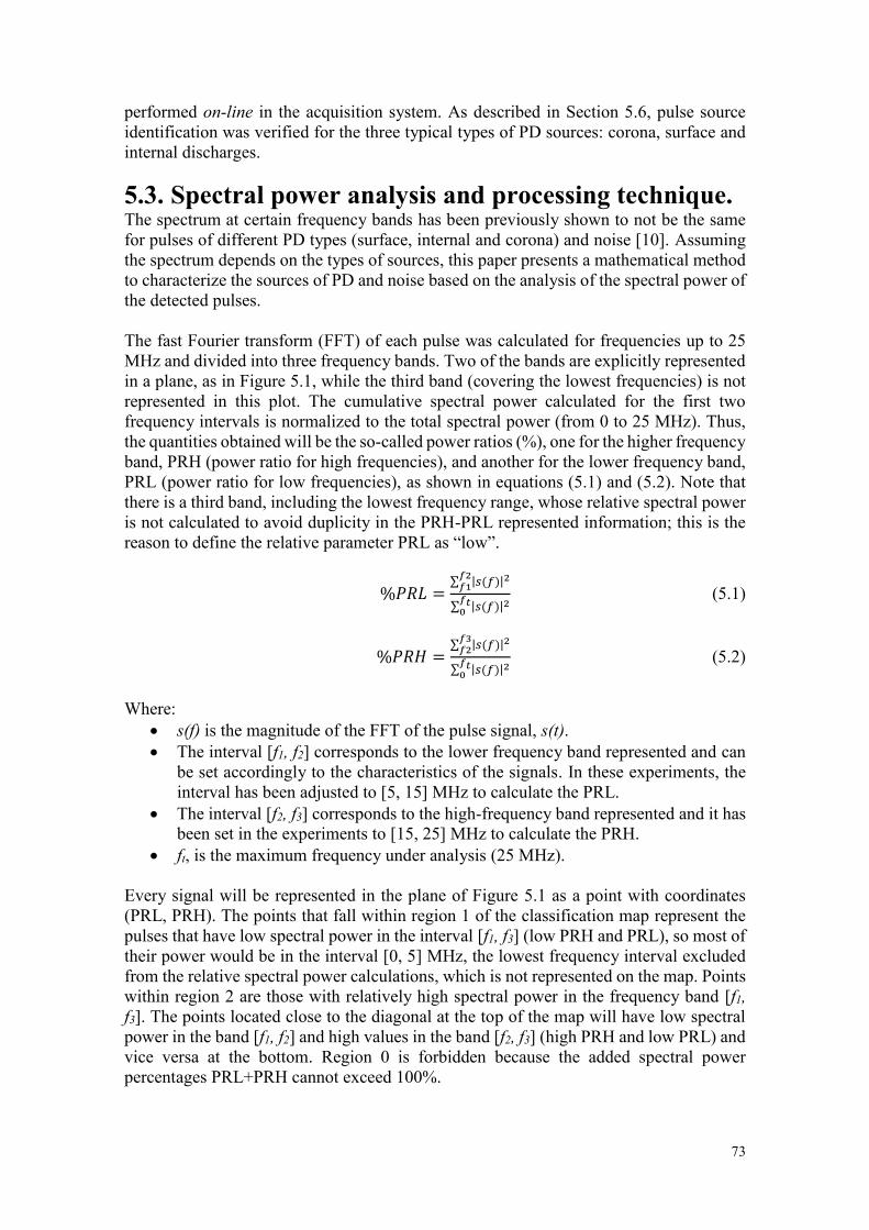
73

performed on-line in the acquisition system. As described in Section 5.6, pulse source identification was verified for the three typical types of PD sources: corona, surface and internal discharges.

5.3. Spectral power analysis and processing technique. The spectrum at certain frequency bands has been previously shown to not be the same for pulses of different PD types (surface, internal and corona) and noise [10]. Assuming the spectrum depends on the types of sources, this paper presents a mathematical method to characterize the sources of PD and noise based on the analysis of the spectral power of the detected pulses. The fast Fourier transform (FFT) of each pulse was calculated for frequencies up to 25 MHz and divided into three frequency bands. Two of the bands are explicitly represented in a plane, as in Figure 5.1, while the third band (covering the lowest frequencies) is not represented in this plot. The cumulative spectral power calculated for the first two frequency intervals is normalized to the total spectral power (from 0 to 25 MHz). Thus, the quantities obtained will be the so-called power ratios (%), one for the higher frequency band, PRH (power ratio for high frequencies), and another for the lower frequency band, PRL (power ratio for low frequencies), as shown in equations (5.1) and (5.2). Note that there is a third band, including the lowest frequency range, whose relative spectral power is not calculated to avoid duplicity in the PRH-PRL represented information; this is the reason to define the relative parameter PRL as “low”.

%𝑃𝑅𝐿 =∑ |𝑠(𝑓)|2𝑓2

𝑓1

∑ |𝑠(𝑓)|2𝑓𝑡0

(5.1)

%𝑃𝑅𝐻 =∑ |𝑠(𝑓)|2𝑓3

𝑓2

∑ |𝑠(𝑓)|2𝑓𝑡0

(5.2)

Where:

s(f) is the magnitude of the FFT of the pulse signal, s(t). The interval [f1, f2] corresponds to the lower frequency band represented and can

be set accordingly to the characteristics of the signals. In these experiments, the interval has been adjusted to [5, 15] MHz to calculate the PRL.

The interval [f2, f3] corresponds to the high-frequency band represented and it has been set in the experiments to [15, 25] MHz to calculate the PRH.

ft, is the maximum frequency under analysis (25 MHz).

Every signal will be represented in the plane of Figure 5.1 as a point with coordinates (PRL, PRH). The points that fall within region 1 of the classification map represent the pulses that have low spectral power in the interval [f1, f3] (low PRH and PRL), so most of their power would be in the interval [0, 5] MHz, the lowest frequency interval excluded from the relative spectral power calculations, which is not represented on the map. Points within region 2 are those with relatively high spectral power in the frequency band [f1, f3]. The points located close to the diagonal at the top of the map will have low spectral power in the band [f1, f2] and high values in the band [f2, f3] (high PRH and low PRL) and vice versa at the bottom. Region 0 is forbidden because the added spectral power percentages PRL+PRH cannot exceed 100%.

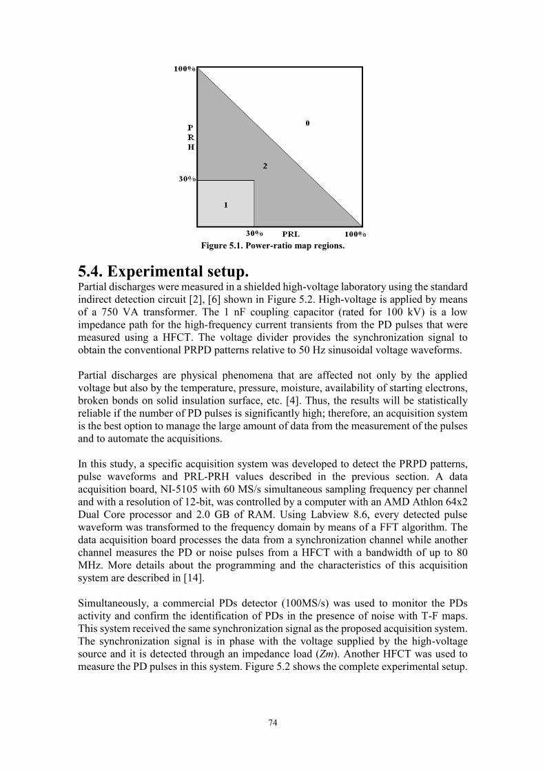
74

Figure 5.1. Power-ratio map regions.

5.4. Experimental setup. Partial discharges were measured in a shielded high-voltage laboratory using the standard indirect detection circuit [2], [6] shown in Figure 5.2. High-voltage is applied by means of a 750 VA transformer. The 1 nF coupling capacitor (rated for 100 kV) is a low impedance path for the high-frequency current transients from the PD pulses that were measured using a HFCT. The voltage divider provides the synchronization signal to obtain the conventional PRPD patterns relative to 50 Hz sinusoidal voltage waveforms. Partial discharges are physical phenomena that are affected not only by the applied voltage but also by the temperature, pressure, moisture, availability of starting electrons, broken bonds on solid insulation surface, etc. [4]. Thus, the results will be statistically reliable if the number of PD pulses is significantly high; therefore, an acquisition system is the best option to manage the large amount of data from the measurement of the pulses and to automate the acquisitions. In this study, a specific acquisition system was developed to detect the PRPD patterns, pulse waveforms and PRL-PRH values described in the previous section. A data acquisition board, NI-5105 with 60 MS/s simultaneous sampling frequency per channel and with a resolution of 12-bit, was controlled by a computer with an AMD Athlon 64x2 Dual Core processor and 2.0 GB of RAM. Using Labview 8.6, every detected pulse waveform was transformed to the frequency domain by means of a FFT algorithm. The data acquisition board processes the data from a synchronization channel while another channel measures the PD or noise pulses from a HFCT with a bandwidth of up to 80 MHz. More details about the programming and the characteristics of this acquisition system are described in [14]. Simultaneously, a commercial PDs detector (100MS/s) was used to monitor the PDs activity and confirm the identification of PDs in the presence of noise with T-F maps. This system received the same synchronization signal as the proposed acquisition system. The synchronization signal is in phase with the voltage supplied by the high-voltage source and it is detected through an impedance load (Zm). Another HFCT was used to measure the PD pulses in this system. Figure 5.2 shows the complete experimental setup.

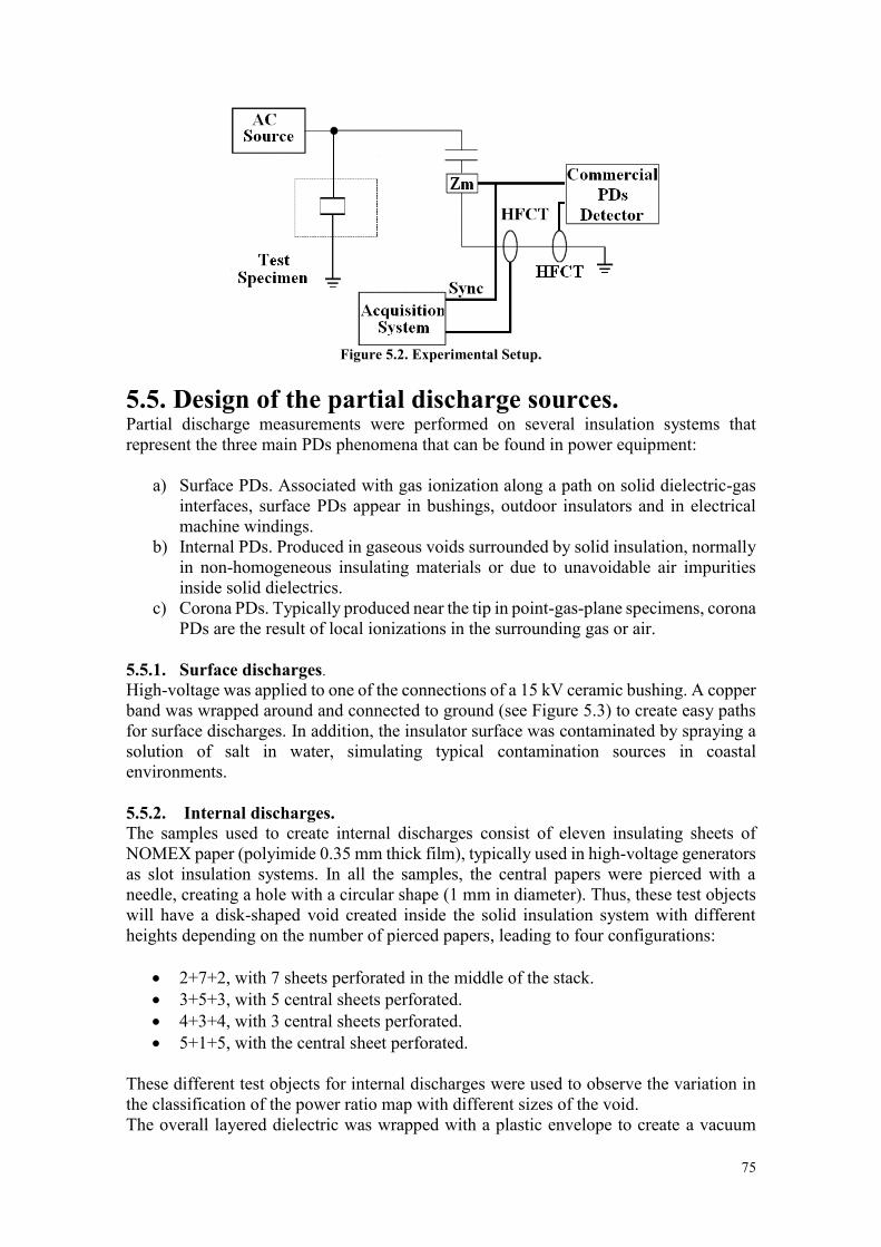
75

Figure 5.2. Experimental Setup.

5.5. Design of the partial discharge sources. Partial discharge measurements were performed on several insulation systems that represent the three main PDs phenomena that can be found in power equipment:

a) Surface PDs. Associated with gas ionization along a path on solid dielectric-gas

interfaces, surface PDs appear in bushings, outdoor insulators and in electrical machine windings.

b) Internal PDs. Produced in gaseous voids surrounded by solid insulation, normally in non-homogeneous insulating materials or due to unavoidable air impurities inside solid dielectrics.

c) Corona PDs. Typically produced near the tip in point-gas-plane specimens, corona PDs are the result of local ionizations in the surrounding gas or air.

5.5.1. Surface discharges. High-voltage was applied to one of the connections of a 15 kV ceramic bushing. A copper band was wrapped around and connected to ground (see Figure 5.3) to create easy paths for surface discharges. In addition, the insulator surface was contaminated by spraying a solution of salt in water, simulating typical contamination sources in coastal environments. 5.5.2. Internal discharges. The samples used to create internal discharges consist of eleven insulating sheets of NOMEX paper (polyimide 0.35 mm thick film), typically used in high-voltage generators as slot insulation systems. In all the samples, the central papers were pierced with a needle, creating a hole with a circular shape (1 mm in diameter). Thus, these test objects will have a disk-shaped void created inside the solid insulation system with different heights depending on the number of pierced papers, leading to four configurations:

2+7+2, with 7 sheets perforated in the middle of the stack. 3+5+3, with 5 central sheets perforated. 4+3+4, with 3 central sheets perforated. 5+1+5, with the central sheet perforated.

These different test objects for internal discharges were used to observe the variation in the classification of the power ratio map with different sizes of the void. The overall layered dielectric was wrapped with a plastic envelope to create a vacuum

76

inside and the entire system was immersed in mineral oil to avoid surface discharges at low voltages. Specimens of this type will guarantee the generation of internal PDs (see Figure 5.4).

5.5.3. Corona discharges. In the corona-discharge specimens, a needle was placed above a wide metallic ground plane. The relative distance between the needle and the plane is adjusted with a screw. The mechanical support is made with Teflon (see Figure 5.5).

Figure 5.3. Surface PDs source. Contaminated ceramic bushing (Experiment # 1).

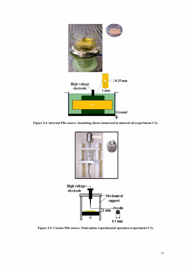
77

Figure 5.4. Internal PDs source. Insulating sheets immersed in mineral oil (experiment # 2).

Figure 5.5. Corona PDs source. Point-plane experimental specimen (experiment # 3).

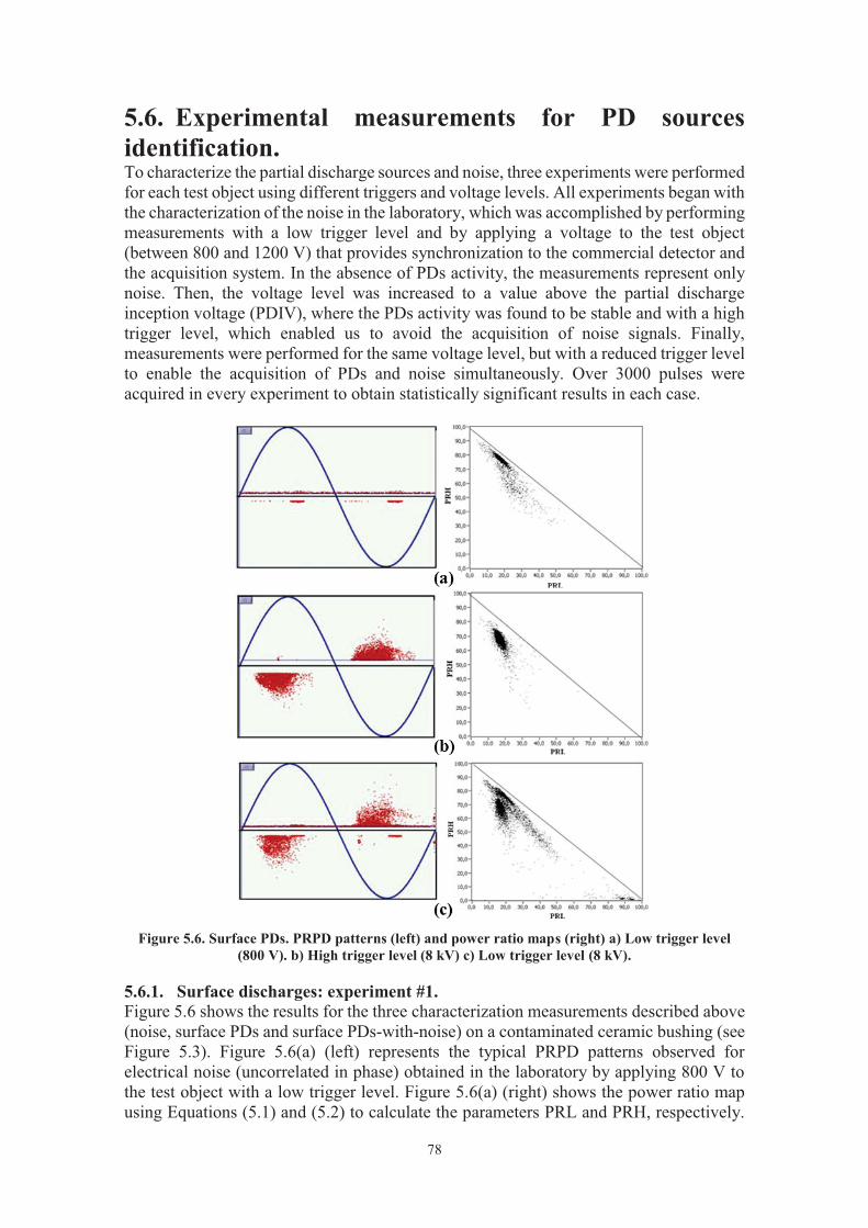
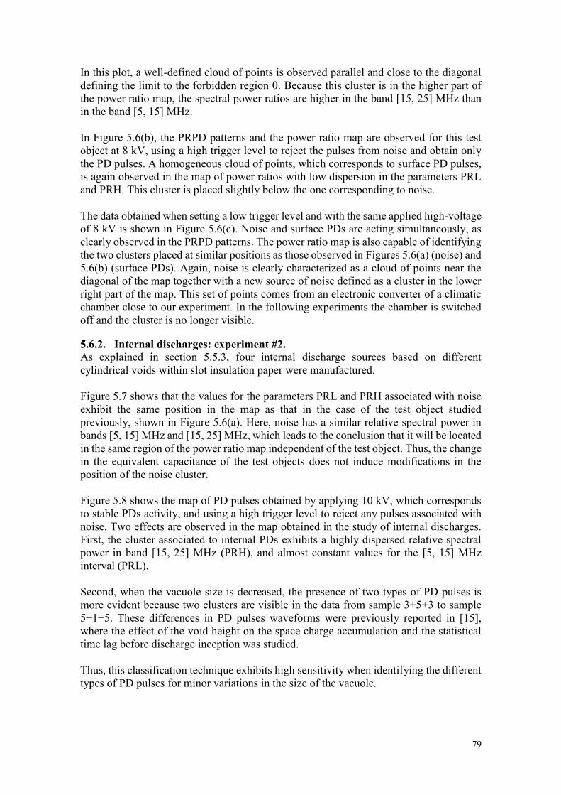
79

In this plot, a well-defined cloud of points is observed parallel and close to the diagonal defining the limit to the forbidden region 0. Because this cluster is in the higher part of the power ratio map, the spectral power ratios are higher in the band [15, 25] MHz than in the band [5, 15] MHz. In Figure 5.6(b), the PRPD patterns and the power ratio map are observed for this test object at 8 kV, using a high trigger level to reject the pulses from noise and obtain only the PD pulses. A homogeneous cloud of points, which corresponds to surface PD pulses, is again observed in the map of power ratios with low dispersion in the parameters PRL and PRH. This cluster is placed slightly below the one corresponding to noise. The data obtained when setting a low trigger level and with the same applied high-voltage of 8 kV is shown in Figure 5.6(c). Noise and surface PDs are acting simultaneously, as clearly observed in the PRPD patterns. The power ratio map is also capable of identifying the two clusters placed at similar positions as those observed in Figures 5.6(a) (noise) and 5.6(b) (surface PDs). Again, noise is clearly characterized as a cloud of points near the diagonal of the map together with a new source of noise defined as a cluster in the lower right part of the map. This set of points comes from an electronic converter of a climatic chamber close to our experiment. In the following experiments the chamber is switched off and the cluster is no longer visible.

5.6.2. Internal discharges: experiment #2. As explained in section 5.5.3, four internal discharge sources based on different cylindrical voids within slot insulation paper were manufactured. Figure 5.7 shows that the values for the parameters PRL and PRH associated with noise exhibit the same position in the map as that in the case of the test object studied previously, shown in Figure 5.6(a). Here, noise has a similar relative spectral power in bands [5, 15] MHz and [15, 25] MHz, which leads to the conclusion that it will be located in the same region of the power ratio map independent of the test object. Thus, the change in the equivalent capacitance of the test objects does not induce modifications in the position of the noise cluster. Figure 5.8 shows the map of PD pulses obtained by applying 10 kV, which corresponds to stable PDs activity, and using a high trigger level to reject any pulses associated with noise. Two effects are observed in the map obtained in the study of internal discharges. First, the cluster associated to internal PDs exhibits a highly dispersed relative spectral power in band [15, 25] MHz (PRH), and almost constant values for the [5, 15] MHz interval (PRL). Second, when the vacuole size is decreased, the presence of two types of PD pulses is more evident because two clusters are visible in the data from sample 3+5+3 to sample 5+1+5. These differences in PD pulses waveforms were previously reported in [15], where the effect of the void height on the space charge accumulation and the statistical time lag before discharge inception was studied. Thus, this classification technique exhibits high sensitivity when identifying the different types of PD pulses for minor variations in the size of the vacuole.

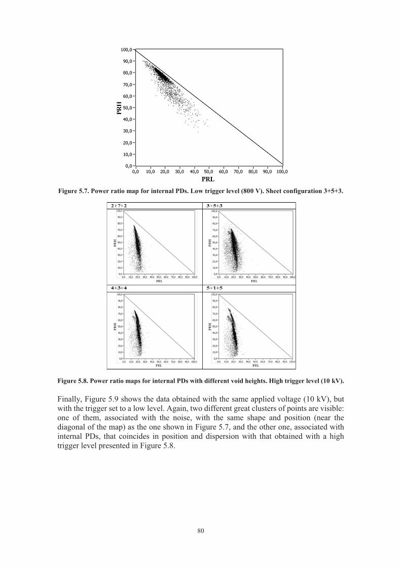
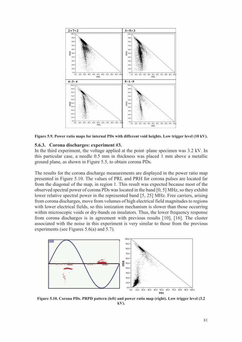
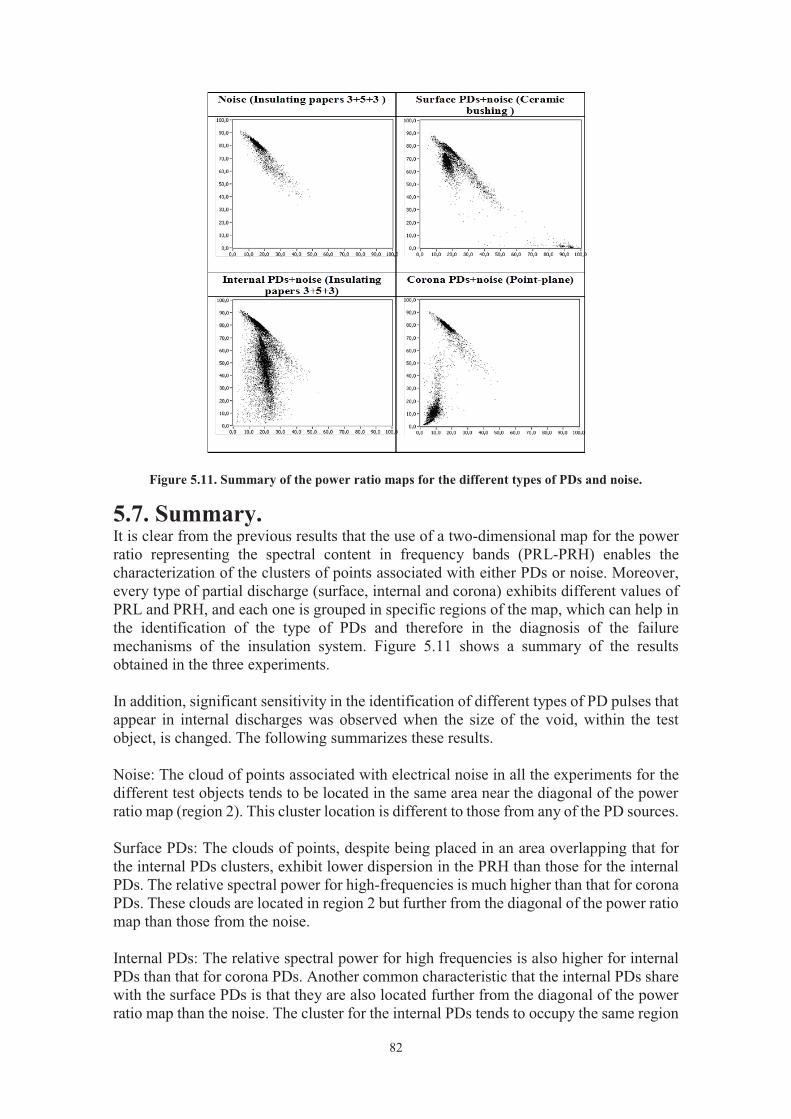
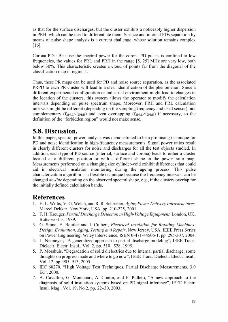
83

as that for the surface discharges, but the cluster exhibits a noticeably higher dispersion in PRH, which can be used to differentiate them. Surface and internal PDs separation by means of pulse shape analysis is a current challenge, whose solution remains complex [16]. Corona PDs: Because the spectral power for the corona PD pulses is confined to low frequencies, the values for PRL and PRH in the range [5, 25] MHz are very low, both below 30%. This characteristic creates a cloud of points far from the diagonal of the classification map in region 1. Thus, these PR maps can be used for PD and noise source separation, as the associated PRPD to each PR cluster will lead to a clear identification of the phenomenon. Since a different experimental configuration or industrial environment might lead to changes in the location of the clusters, this system allows the operator to modify the calculation intervals depending on pulse spectrum shape. Moreover, PRH and PRL calculation intervals might be different (depending on the sampling frequency and used sensor), not complementary (f2PRL<f2PRH) and even overlapping (f2PRL>f2PRH) if necessary, so the definition of the “forbidden region” would not make sense. 5.8. Discussion. In this paper, spectral power analysis was demonstrated to be a promising technique for PD and noise identification in high-frequency measurements. Signal power ratios result in clearly different clusters for noise and discharges for all the test objects studied. In addition, each type of PD source (internal, surface and corona) leads to either a cluster located at a different position or with a different shape in the power ratio map. Measurements performed on a changing size cylinder-void exhibit differences that could aid in electrical insulation monitoring during the ageing process. This pulse characterization algorithm is a flexible technique because the frequency intervals can be changed on-line depending on the observed spectral shape, e.g., if the clusters overlap for the initially defined calculation bands. References 1. H. L. Willis, V. G. Welch, and R. R. Schrieber, Aging Power Delivery Infrastructures,

Marcel Dekker, New York, USA, pp. 210-225, 2001. 2. F. H. Kreuger, Partial Discharge Detection in High-Voltage Equipment, London, UK,

Butterworths, 1989. 3. G. Stone, E. Boutler and I. Culbert, Electrical Insulation for Rotating Machines:

Design, Evaluation, Aging, Testing and Repair, New Jersey, USA, IEEE Press Series on Power Engineering, Wiley Interscience, ISBN 0-471-44506-1, pp. 295-307, 2004.

4. L. Niemeyer, “A generalized approach to partial discharge modeling”, IEEE Trans. Dielectr. Electr. Insul., Vol. 2, pp. 510 –528, 1995.

5. P. Morshuis, “Degradation of solid dielectrics due to internal partial discharge: some thoughts on progress made and where to go now”, IEEE Trans. Dielectr. Electr. Insul., Vol. 12, pp. 905–913, 2005.

6. IEC 60270, “High Voltage Test Techniques. Partial Discharge Measurements, 3.0 Ed”, 2000.

7. A. Cavallini, G. Montanari, A. Contin, and F. Pulletti, “A new approach to the diagnosis of solid insulation systems based on PD signal inference”, IEEE Electr. Insul. Mag., Vol. 19, No.2, pp. 22–30, 2003.

84

8. P. Bidan, T. Lebey and C. Neacsu, "Development of a new off-line test procedure for low voltage rotating machines fed by adjustable speed drives (ASD)", IEEE Trans. Dielectr. Electr. Insul., Vol. 10, pp. 168- 175, 2003.

9. IEC/TS 60034-27-2, “Rotating electrical machines- Part 27-2: On-line partial discharge measurements on the stator winding insulation of rotating electrical machines”, Ed. 1.0, 2012.

10. J. M. Martínez-Tarifa, G. Robles, M. V. Rojas-Moreno, and J. Sanz- Feito, “Partial discharge pulse shape recognition using an inductive loop sensor”, Measurement Sci. Techn., Vol. 21, p. 105706, 2010.

11. H. Okubo and N. Hayakawa, “A Novel Technique for Partial Discharge and Breakdown Investigation Based on Current Pulse Waveform Analysis”, IEEE Trans. Dielectr. Electr. Insul., Vol. 12, pp 736-744, 2005.

12. L. Hao, P.L. Lewin, J.A. Hunter, D.J. Swaffield, A. Contin, C. Walton, and M. Michel, "Discrimination of multiple PD sources using wavelet decomposition and principal component analysis," IEEE Trans. Dielectr. Electr. Insul., Vol. 18, pp.1702-1711, 2011.

13. A. Contin, A. Cavallini, G.C. Montanari, G. Pasini and F. Puletti, "Digital detection and fuzzy classification of partial discharge signals," IEEE Trans. Dielectr. Electr. Insul., Vol. 9, pp.335-348, 2002.

14. J.A. Ardila-Rey, J.M. Martinez-Tarifa, G. Robles, M. Rojas-Moreno, and R. Albarracin, "A Partial Discharges acquisition and statistical analysis software", IEEE Int’l. Instrumentation and Measurement Technology Conf. (MTC), pp.1670-1675, 2012.

15. P. Morshuis, Partial Discharge Mechanisms, Ph.D. degree thesis, Delft University Press, Netherlands, 1993.

16. A. Cavallini, G.C. Montanari, M. Tozzi and X. Chen, "Diagnostic of HVDC systems using partial discharges", IEEE Trans. Dielectr. Electr. Insul, Vol.18, pp.275-284, 2011.

85

Chapter 6

Partial Discharge Source Recognition by Means of Spectral Power Ratios

Clustering Contents 6.1. Abstract .................................................................................................................... 85 6.2. Introduction ............................................................................................................. 85 6.3. The power ratios map .............................................................................................. 87 6.4. Experimental setup .................................................................................................. 88 6.5. Partial discharge source separation in the designed test objects ............................. 90 6.5.1. Internal and corona discharges ........................................................................... 90 6.5.2. Internal and surface discharges ........................................................................... 92

6.6. Partial discharge detection in an insulated power cable .......................................... 95 6.7. Discussion ................................................................................................................ 98 References ...................................................................................................................... 98

6.1. Abstract. Partial discharge (PD) detection can give useful information for the diagnosis of electrical apparatuses, but data interpretation can be impossible if several sources are simultaneously active. Pulse characterization can be used to identify the source origin in PD measurements. The distribution of energy at different frequencies helps to distinguish between several types of discharges. The parameterization of pulses by means of spectral power ratios (PR) has been studied as a reliable technique to represent different characteristics in high-frequency current pulses in high-voltage tests. In this study, the separation of partial discharge sources by means of power ratios maps is proposed. This approach has proven to be effective in the identification of PD sources when two electrical insulation systems are simultaneously subjected to discharge activity in controlled experiments where internal, surface and corona discharges were occurring. The flexibility of the system to improve cluster separation is shown, and measurements are also made on a real insulated power cable, where two simultaneous PD sources were successfully identified.

6.2. Introduction. Several degradation mechanisms can lead to unexpected failures in the electrical insulation of electrical machines and power cables [1]. The power disruption and the replacement of expensive equipment that result from unexpected failures can represent high costs for utilities. Thus, predictive maintenance arises as an industrial strategic topic for the power grid. Among several techniques, partial discharge activity has been proven

86

to be an effective diagnosis tool to detect electrical, thermal, and mechanical stresses in all these power assets [2]. Partial discharges (PDs) are microscopic ionizations that take place within insulation volumes due to high electrical field divergences. This phenomenon involves low energy emissions, so it will not cause immediate failures; however, the repeated occurrence of PDs (several times per power cycle) may degrade solid or liquid insulation systems, leading to their ultimate breakdown [3], [4]. For all of these reasons, partial discharge detection has become an interesting issue for researchers and asset managers. The classical measurement systems represent PD pulse magnitudes on the applied voltage phase to identify the PD source by means of the partial discharge phase resolved (PRPD) pattern [5]. These detection systems are able to identify several types of PD sources in a limited bandwidth (100 – 500 kHz) with only capacitive dividers to detect PD pulses and a synchronization voltage [2], [4], [6], [7], [8] and [9]. However, if the signal-to-noise ratio (SNR) is very low or if several PD sources are simultaneously active, PD recognition by means of PRPD patterns may be impossible [10]. As PD monitoring is usually performed on-line, several stresses may lead to different PD active sites, which may overlap on the PRPD diagrams. Moreover, not all PD sources may be harmful for the insulation bulk, and a first PD classification must be taken into account [8]:

a) Internal PDs are the result of microscopic voids within solid or liquid insulation systems. As these voids are usually filled with materials of lower breakdown strengths and permittivity, the ionizations are limited to voids, whose surfaces will be degraded through physical and chemical attack. Thus, internal PDs are usually harmful for the insulation system or may indicate voids created by other thermal or mechanical stresses.

b) Surface PDs are ionizations that propagate perpendicularly to the applied field, usually in metal-air-solid insulation interfaces. They are typical in contaminated insulators or bushings and their detection could help to locate the source and mitigate their presence; for example, if they are found in an electrical machine, cleaning bushing surfaces may eliminate this PD activity.

c) Corona PDs are ionizations that occur as a consequence of sharp metallic electrodes. In some cases, these sources may come from loose threads in high-voltage connections, which are not an immediate threat to the equipment and, if detected, could be easily corrected.

There is a considerable amount of literature on identifying these PD sources by means of PRPD patterns [7], [8], [9], but, as stated before, their interpretation is sometimes impossible. To address this problem, PD pulse waveform analysis has been proposed to filter the pulse acquisitions. For this purpose, broadband detection (up to 100 MHz) by means of inductive devices [11] has been applied because they can make use of the PRPD patterns and the PD current waveform analysis in the standard detection circuits [10], [12]. Among the several technical approaches that have been applied to classify PD pulses, the Time-Frequency (T-F) maps have led to one of the most successful solutions ([10]), but the parameters used to classify PD pulses are fixed and cannot be changed by the user.

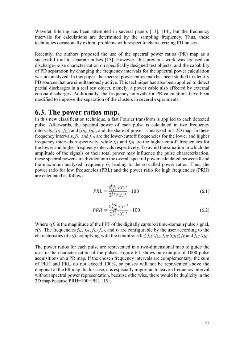
87

Wavelet filtering has been attempted in several papers [13], [14], but the frequency intervals for calculations are determined by the sampling frequency. Thus, these techniques occasionally exhibit problems with respect to characterizing PD pulses. Recently, the authors proposed the use of the spectral power ratios (PR) map as a successful tool to separate pulses [15]. However, this previous work was focused on discharge-noise characterization on specifically designed test objects, and the capability of PD separation by changing the frequency intervals for the spectral power calculation was not analyzed. In this paper, the spectral power ratios map has been studied to identify PD sources that are simultaneously active. This technique has also been applied to detect partial discharges in a real test object, namely, a power cable also affected by external corona discharges. Additionally, the frequency intervals for PR calculations have been modified to improve the separation of the clusters in several experiments.

6.3. The power ratios map. In this new classification technique, a fast Fourier transform is applied to each detected pulse. Afterwards, the spectral power of each pulse is calculated in two frequency intervals, [f1L, f2L] and [f1H, f2H], and the share of power is analyzed in a 2D map. In these frequency intervals, f1L and f1H are the lower-cuttoff frequencies for the lower and higher frequency intervals respectively, while f2L and f2H are the higher-cuttoff frequencies for the lower and higher frequency intervals respectively. To avoid the situation in which the amplitude of the signals or their total power may influence the pulse characterization, these spectral powers are divided into the overall spectral power calculated between 0 and the maximum analyzed frequency fT, leading to the so-called power ratios. Thus, the power ratio for low frequencies (PRL) and the power ratio for high frequencies (PRH) are calculated as follows:

𝑃𝑅𝐿 =∑ |𝑠(𝑓)|2f2L

𝑓1𝐿

∑ |𝑠(𝑓)|2𝑓𝑇0

· 100 (6.1)


𝑓1𝐻

∑ |𝑠(𝑓)|2𝑓𝑇0

· 100 (6.2)

Where s(f) is the magnitude of the FFT of the digitally captured time-domain pulse signal, s(t). The frequencies f1L, f2L, f1H, f2H, and fT are configurable by the user according to the characteristics of s(f), complying with the conditions 0 ≤ f1L<f2L, f1H<f2H ≤ fT, and f1L<f2H. The power ratios for each pulse are represented in a two-dimensional map to guide the user in the characterization of the pulses. Figure 6.1 shows an example of 1000 pulse acquisitions on a PR map. If the chosen frequency intervals are complementary, the sum of PRH and PRL do not exceed 100%, so pulses will not be represented above the diagonal of the PR map. In this case, it is especially important to leave a frequency interval without spectral power representation, because otherwise, there would be duplicity in the 2D map because PRH=100−PRL [15].

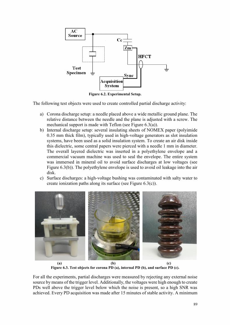
89


The following test objects were used to create controlled partial discharge activity:

a) Corona discharge setup: a needle placed above a wide metallic ground plane. The relative distance between the needle and the plane is adjusted with a screw. The mechanical support is made with Teflon (see Figure 6.3(a)).

b) Internal discharge setup: several insulating sheets of NOMEX paper (polyimide 0.35 mm thick film), typically used in high-voltage generators as slot insulation systems, have been used as a solid insulation system. To create an air disk inside this dielectric, some central papers were pierced with a needle 1 mm in diameter. The overall layered dielectric was inserted in a polyethylene envelope and a commercial vacuum machine was used to seal the envelope. The entire system was immersed in mineral oil to avoid surface discharges at low voltages (see Figure 6.3(b)). The polyethylene envelope is used to avoid oil leakage into the air disk.

c) Surface discharges: a high-voltage bushing was contaminated with salty water to create ionization paths along its surface (see Figure 6.3(c)).

(a) (b) (c)

Figure 6.3. Test objects for corona PD (a), internal PD (b), and surface PD (c).

For all the experiments, partial discharges were measured by rejecting any external noise source by means of the trigger level. Additionally, the voltages were high enough to create PDs well above the trigger level below which the noise is present, so a high SNR was achieved. Every PD acquisition was made after 15 minutes of stable activity. A minimum

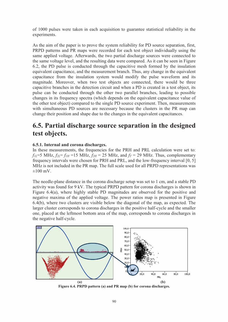
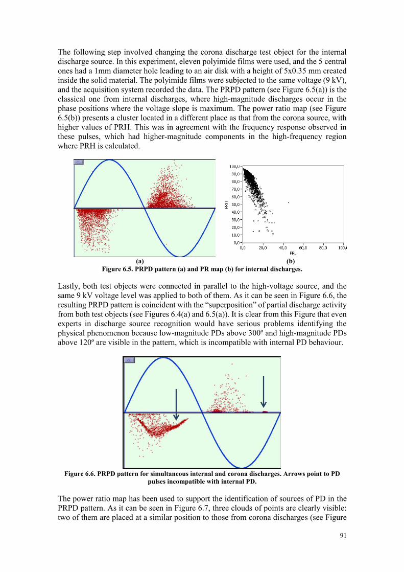
91

The following step involved changing the corona discharge test object for the internal discharge source. In this experiment, eleven polyimide films were used, and the 5 central ones had a 1mm diameter hole leading to an air disk with a height of 5x0.35 mm created inside the solid material. The polyimide films were subjected to the same voltage (9 kV), and the acquisition system recorded the data. The PRPD pattern (see Figure 6.5(a)) is the classical one from internal discharges, where high-magnitude discharges occur in the phase positions where the voltage slope is maximum. The power ratio map (see Figure 6.5(b)) presents a cluster located in a different place as that from the corona source, with higher values of PRH. This was in agreement with the frequency response observed in these pulses, which had higher-magnitude components in the high-frequency region where PRH is calculated.

(a) (b)

Figure 6.5. PRPD pattern (a) and PR map (b) for internal discharges. Lastly, both test objects were connected in parallel to the high-voltage source, and the same 9 kV voltage level was applied to both of them. As it can be seen in Figure 6.6, the resulting PRPD pattern is coincident with the “superposition” of partial discharge activity from both test objects (see Figures 6.4(a) and 6.5(a)). It is clear from this Figure that even experts in discharge source recognition would have serious problems identifying the physical phenomenon because low-magnitude PDs above 300º and high-magnitude PDs above 120º are visible in the pattern, which is incompatible with internal PD behaviour.

Figure 6.6. PRPD pattern for simultaneous internal and corona discharges. Arrows point to PD

pulses incompatible with internal PD. The power ratio map has been used to support the identification of sources of PD in the PRPD pattern. As it can be seen in Figure 6.7, three clouds of points are clearly visible: two of them are placed at a similar position to those from corona discharges (see Figure

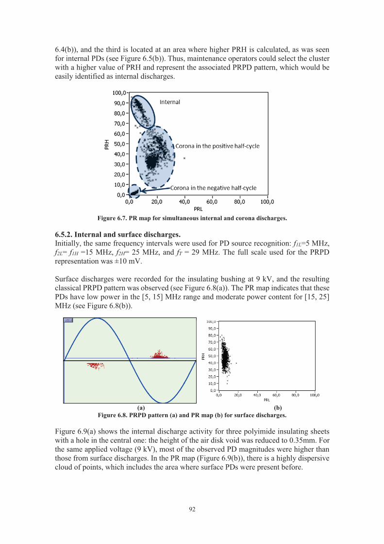
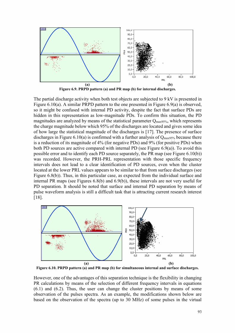
93

(a) (b)

Figure 6.9. PRPD pattern (a) and PR map (b) for internal discharges.

The partial discharge activity when both test objects are subjected to 9 kV is presented in Figure 6.10(a). A similar PRPD pattern to the one presented in Figure 6.9(a) is observed, so it might be confused with internal PD activity, despite the fact that surface PDs are hidden in this representation as low-magnitude PDs. To confirm this situation, the PD magnitudes are analyzed by means of the statistical parameter Qmax95%, which represents the charge magnitude below which 95% of the discharges are located and gives some idea of how large the statistical magnitude of the discharges is [17]. The presence of surface discharges in Figure 6.10(a) is confirmed with a further analysis of Qmax95% because there is a reduction of its magnitude of 4% (for negative PDs) and 9% (for positive PDs) when both PD sources are active compared with internal PD (see Figure 6.9(a)). To avoid this possible error and to identify each PD source separately, the PR map (see Figure 6.10(b)) was recorded. However, the PRH-PRL representation with those specific frequency intervals does not lead to a clear identification of PD sources, even when the cluster located at the lower PRL values appears to be similar to that from surface discharges (see Figure 6.8(b)). Thus, in this particular case, as expected from the individual surface and internal PR maps (see Figures 6.8(b) and 6.9(b)), these intervals are not very useful for PD separation. It should be noted that surface and internal PD separation by means of pulse waveform analysis is still a difficult task that is attracting current research interest [18].

(a) (b)

Figure 6.10. PRPD pattern (a) and PR map (b) for simultaneous internal and surface discharges. However, one of the advantages of this separation technique is the flexibility in changing PR calculations by means of the selection of different frequency intervals in equations (6.1) and (6.2). Thus, the user can change the cluster positions by means of some observation of the pulses spectra. As an example, the modifications shown below are based on the observation of the spectra (up to 30 MHz) of some pulses in the virtual

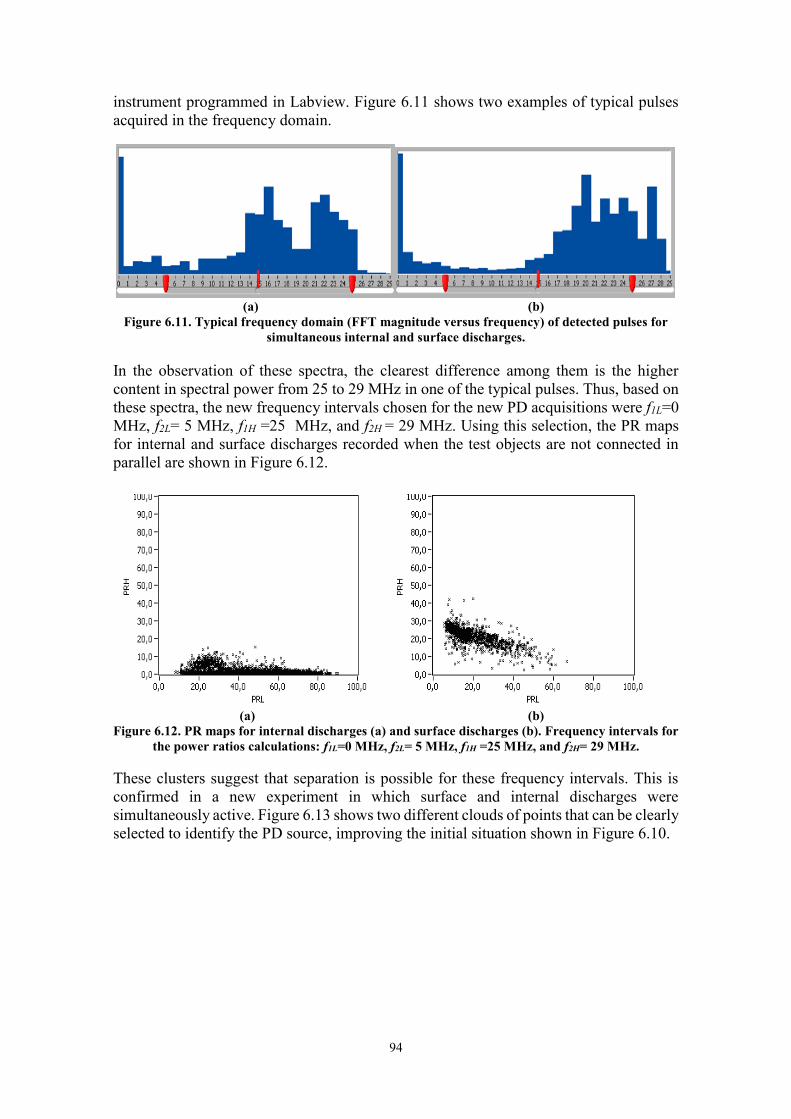
94

instrument programmed in Labview. Figure 6.11 shows two examples of typical pulses acquired in the frequency domain.

(a) (b)

Figure 6.11. Typical frequency domain (FFT magnitude versus frequency) of detected pulses for simultaneous internal and surface discharges.

In the observation of these spectra, the clearest difference among them is the higher content in spectral power from 25 to 29 MHz in one of the typical pulses. Thus, based on these spectra, the new frequency intervals chosen for the new PD acquisitions were f1L=0 MHz, f2L= 5 MHz, f1H =25 MHz, and f2H = 29 MHz. Using this selection, the PR maps for internal and surface discharges recorded when the test objects are not connected in parallel are shown in Figure 6.12.

(a) (b) Figure 6.12. PR maps for internal discharges (a) and surface discharges (b). Frequency intervals for

the power ratios calculations: f1L=0 MHz, f2L= 5 MHz, f1H =25 MHz, and f2H= 29 MHz.

These clusters suggest that separation is possible for these frequency intervals. This is confirmed in a new experiment in which surface and internal discharges were simultaneously active. Figure 6.13 shows two different clouds of points that can be clearly selected to identify the PD source, improving the initial situation shown in Figure 6.10.

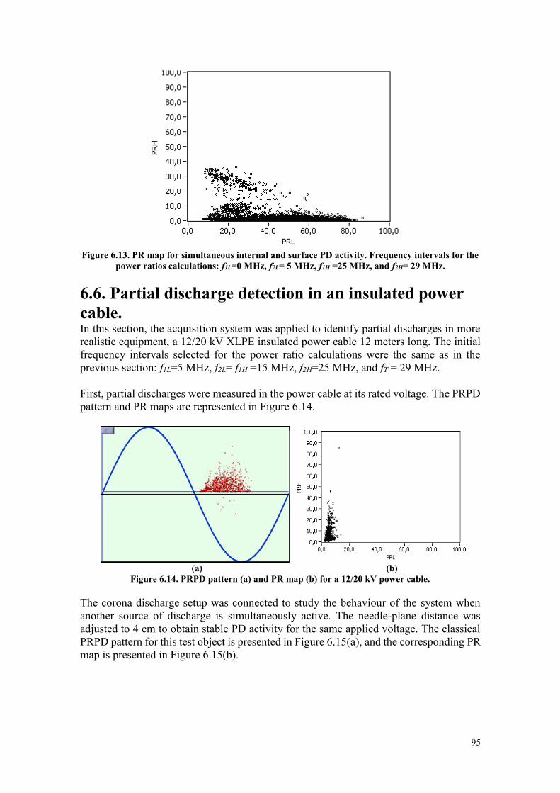
95

Figure 6.13. PR map for simultaneous internal and surface PD activity. Frequency intervals for the

power ratios calculations: f1L=0 MHz, f2L= 5 MHz, f1H =25 MHz, and f2H= 29 MHz.

6.6. Partial discharge detection in an insulated power cable. In this section, the acquisition system was applied to identify partial discharges in more realistic equipment, a 12/20 kV XLPE insulated power cable 12 meters long. The initial frequency intervals selected for the power ratio calculations were the same as in the previous section: f1L=5 MHz, f2L= f1H =15 MHz, f2H=25 MHz, and fT = 29 MHz. First, partial discharges were measured in the power cable at its rated voltage. The PRPD pattern and PR maps are represented in Figure 6.14.

(a) (b)

Figure 6.14. PRPD pattern (a) and PR map (b) for a 12/20 kV power cable. The corona discharge setup was connected to study the behaviour of the system when another source of discharge is simultaneously active. The needle-plane distance was adjusted to 4 cm to obtain stable PD activity for the same applied voltage. The classical PRPD pattern for this test object is presented in Figure 6.15(a), and the corresponding PR map is presented in Figure 6.15(b).

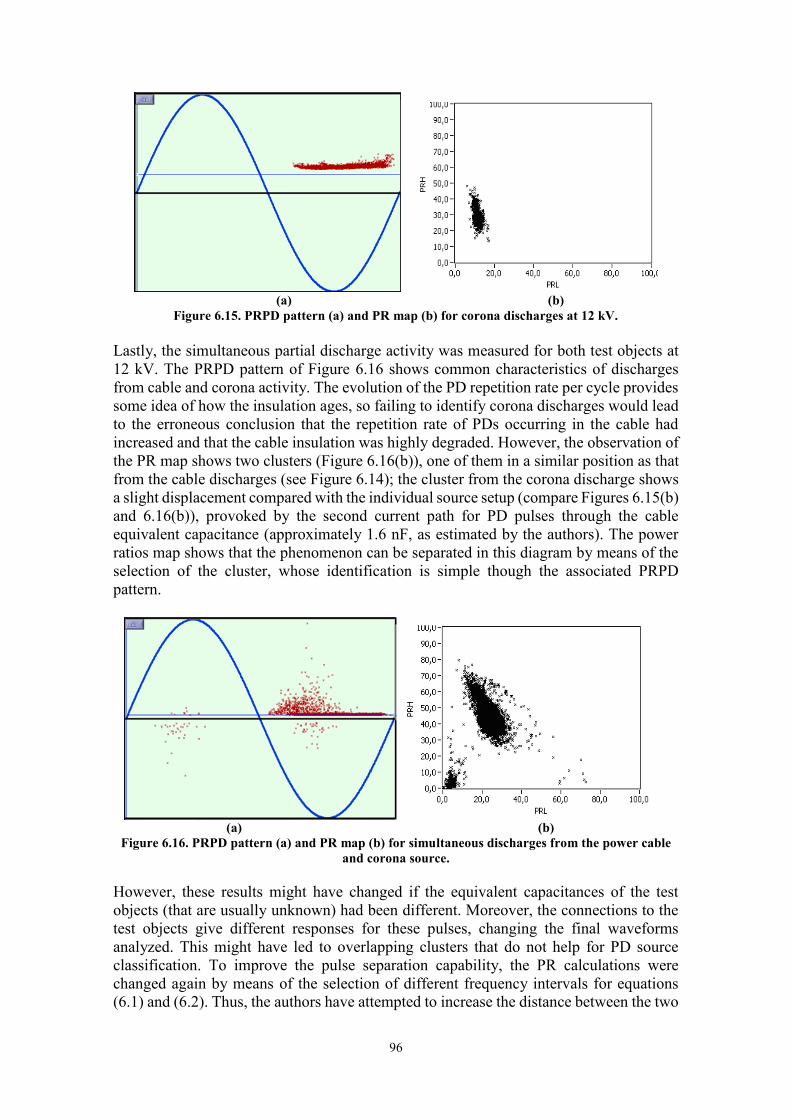
96

(a) (b)

Figure 6.15. PRPD pattern (a) and PR map (b) for corona discharges at 12 kV. Lastly, the simultaneous partial discharge activity was measured for both test objects at 12 kV. The PRPD pattern of Figure 6.16 shows common characteristics of discharges from cable and corona activity. The evolution of the PD repetition rate per cycle provides some idea of how the insulation ages, so failing to identify corona discharges would lead to the erroneous conclusion that the repetition rate of PDs occurring in the cable had increased and that the cable insulation was highly degraded. However, the observation of the PR map shows two clusters (Figure 6.16(b)), one of them in a similar position as that from the cable discharges (see Figure 6.14); the cluster from the corona discharge shows a slight displacement compared with the individual source setup (compare Figures 6.15(b) and 6.16(b)), provoked by the second current path for PD pulses through the cable equivalent capacitance (approximately 1.6 nF, as estimated by the authors). The power ratios map shows that the phenomenon can be separated in this diagram by means of the selection of the cluster, whose identification is simple though the associated PRPD pattern.

(a) (b)

Figure 6.16. PRPD pattern (a) and PR map (b) for simultaneous discharges from the power cable and corona source.

However, these results might have changed if the equivalent capacitances of the test objects (that are usually unknown) had been different. Moreover, the connections to the test objects give different responses for these pulses, changing the final waveforms analyzed. This might have led to overlapping clusters that do not help for PD source classification. To improve the pulse separation capability, the PR calculations were changed again by means of the selection of different frequency intervals for equations (6.1) and (6.2). Thus, the authors have attempted to increase the distance between the two

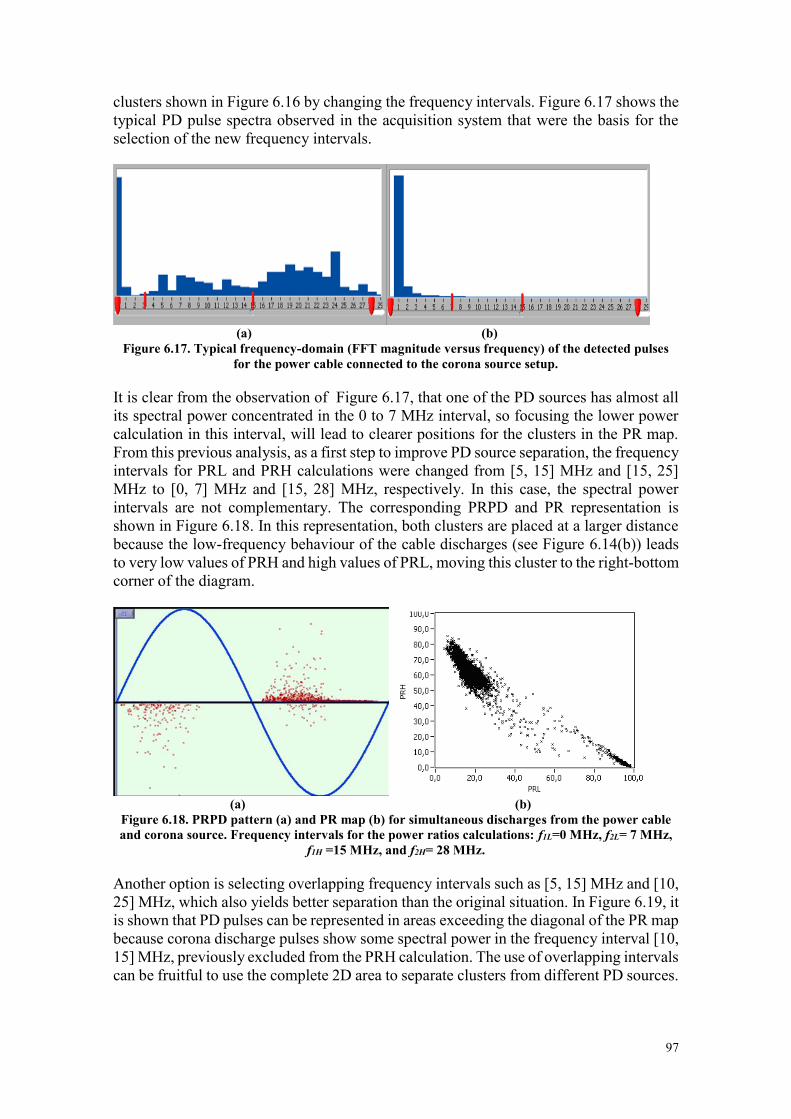
97

clusters shown in Figure 6.16 by changing the frequency intervals. Figure 6.17 shows the typical PD pulse spectra observed in the acquisition system that were the basis for the selection of the new frequency intervals.

(a) (b)

Figure 6.17. Typical frequency-domain (FFT magnitude versus frequency) of the detected pulses for the power cable connected to the corona source setup.

It is clear from the observation of Figure 6.17, that one of the PD sources has almost all its spectral power concentrated in the 0 to 7 MHz interval, so focusing the lower power calculation in this interval, will lead to clearer positions for the clusters in the PR map. From this previous analysis, as a first step to improve PD source separation, the frequency intervals for PRL and PRH calculations were changed from [5, 15] MHz and [15, 25] MHz to [0, 7] MHz and [15, 28] MHz, respectively. In this case, the spectral power intervals are not complementary. The corresponding PRPD and PR representation is shown in Figure 6.18. In this representation, both clusters are placed at a larger distance because the low-frequency behaviour of the cable discharges (see Figure 6.14(b)) leads to very low values of PRH and high values of PRL, moving this cluster to the right-bottom corner of the diagram.

(a) (b)

Figure 6.18. PRPD pattern (a) and PR map (b) for simultaneous discharges from the power cable and corona source. Frequency intervals for the power ratios calculations: f1L=0 MHz, f2L= 7 MHz,

f1H =15 MHz, and f2H= 28 MHz.

Another option is selecting overlapping frequency intervals such as [5, 15] MHz and [10, 25] MHz, which also yields better separation than the original situation. In Figure 6.19, it is shown that PD pulses can be represented in areas exceeding the diagonal of the PR map because corona discharge pulses show some spectral power in the frequency interval [10, 15] MHz, previously excluded from the PRH calculation. The use of overlapping intervals can be fruitful to use the complete 2D area to separate clusters from different PD sources.

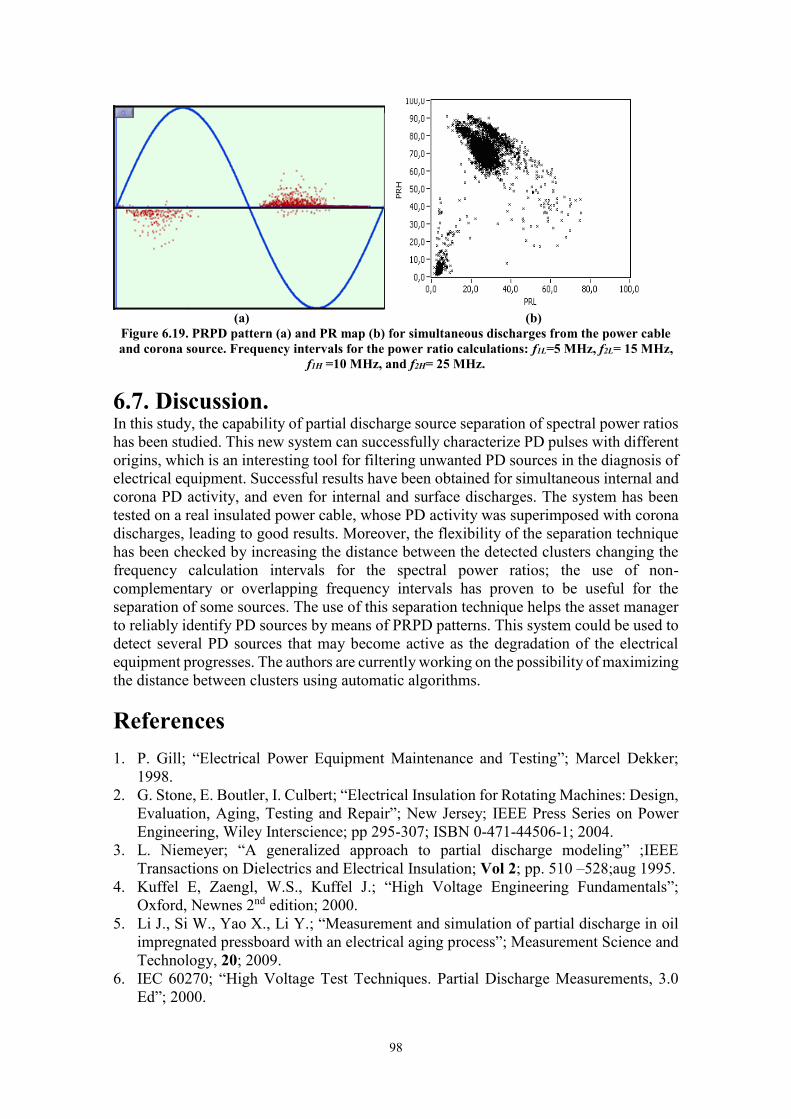
98

(a) (b)

Figure 6.19. PRPD pattern (a) and PR map (b) for simultaneous discharges from the power cable and corona source. Frequency intervals for the power ratio calculations: f1L=5 MHz, f2L= 15 MHz,

f1H =10 MHz, and f2H= 25 MHz.

6.7. Discussion. In this study, the capability of partial discharge source separation of spectral power ratios has been studied. This new system can successfully characterize PD pulses with different origins, which is an interesting tool for filtering unwanted PD sources in the diagnosis of electrical equipment. Successful results have been obtained for simultaneous internal and corona PD activity, and even for internal and surface discharges. The system has been tested on a real insulated power cable, whose PD activity was superimposed with corona discharges, leading to good results. Moreover, the flexibility of the separation technique has been checked by increasing the distance between the detected clusters changing the frequency calculation intervals for the spectral power ratios; the use of non-complementary or overlapping frequency intervals has proven to be useful for the separation of some sources. The use of this separation technique helps the asset manager to reliably identify PD sources by means of PRPD patterns. This system could be used to detect several PD sources that may become active as the degradation of the electrical equipment progresses. The authors are currently working on the possibility of maximizing the distance between clusters using automatic algorithms.

References 1. P. Gill; “Electrical Power Equipment Maintenance and Testing”; Marcel Dekker;

1998. 2. G. Stone, E. Boutler, I. Culbert; “Electrical Insulation for Rotating Machines: Design,

Evaluation, Aging, Testing and Repair”; New Jersey; IEEE Press Series on Power Engineering, Wiley Interscience; pp 295-307; ISBN 0-471-44506-1; 2004.

3. L. Niemeyer; “A generalized approach to partial discharge modeling” ;IEEE Transactions on Dielectrics and Electrical Insulation; Vol 2; pp. 510 –528;aug 1995.

4. Kuffel E, Zaengl, W.S., Kuffel J.; “High Voltage Engineering Fundamentals”; Oxford, Newnes 2nd edition; 2000.

5. Li J., Si W., Yao X., Li Y.; “Measurement and simulation of partial discharge in oil impregnated pressboard with an electrical aging process”; Measurement Science and Technology, 20; 2009.

6. IEC 60270; “High Voltage Test Techniques. Partial Discharge Measurements, 3.0 Ed”; 2000.

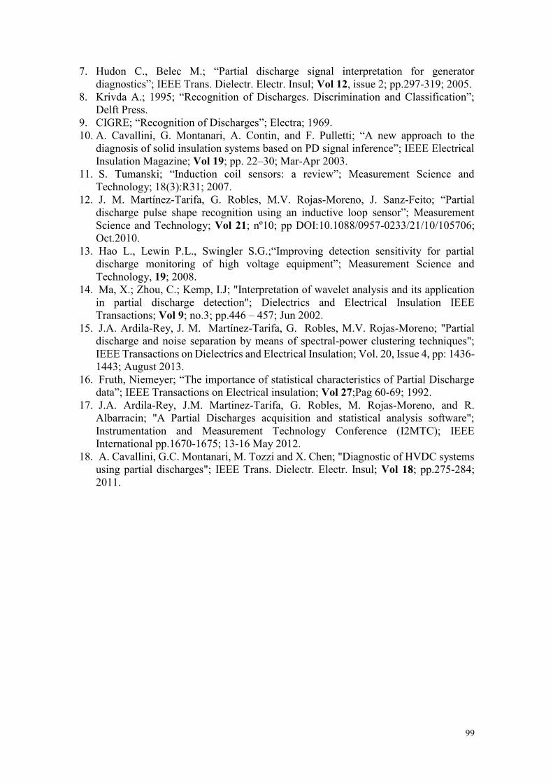
99

7. Hudon C., Belec M.; “Partial discharge signal interpretation for generator diagnostics”; IEEE Trans. Dielectr. Electr. Insul; Vol 12, issue 2; pp.297-319; 2005.

8. Krivda A.; 1995; “Recognition of Discharges. Discrimination and Classification”; Delft Press.

9. CIGRE; “Recognition of Discharges”; Electra; 1969. 10. A. Cavallini, G. Montanari, A. Contin, and F. Pulletti; “A new approach to the

diagnosis of solid insulation systems based on PD signal inference”; IEEE Electrical Insulation Magazine; Vol 19; pp. 22–30; Mar-Apr 2003.

11. S. Tumanski; “Induction coil sensors: a review”; Measurement Science and Technology; 18(3):R31; 2007.

12. J. M. Martínez-Tarifa, G. Robles, M.V. Rojas-Moreno, J. Sanz-Feito; “Partial discharge pulse shape recognition using an inductive loop sensor”; Measurement Science and Technology; Vol 21; nº10; pp DOI:10.1088/0957-0233/21/10/105706; Oct.2010.

13. Hao L., Lewin P.L., Swingler S.G.;“Improving detection sensitivity for partial discharge monitoring of high voltage equipment”; Measurement Science and Technology, 19; 2008.

14. Ma, X.; Zhou, C.; Kemp, I.J; "Interpretation of wavelet analysis and its application in partial discharge detection"; Dielectrics and Electrical Insulation IEEE Transactions; Vol 9; no.3; pp.446 – 457; Jun 2002.

15. J.A. Ardila-Rey, J. M. Martínez-Tarifa, G. Robles, M.V. Rojas-Moreno; "Partial discharge and noise separation by means of spectral-power clustering techniques"; IEEE Transactions on Dielectrics and Electrical Insulation; Vol. 20, Issue 4, pp: 1436-1443; August 2013.

16. Fruth, Niemeyer; “The importance of statistical characteristics of Partial Discharge data”; IEEE Transactions on Electrical insulation; Vol 27;Pag 60-69; 1992.

17. J.A. Ardila-Rey, J.M. Martinez-Tarifa, G. Robles, M. Rojas-Moreno, and R. Albarracin; "A Partial Discharges acquisition and statistical analysis software"; Instrumentation and Measurement Technology Conference (I2MTC); IEEE International pp.1670-1675; 13-16 May 2012.

18. A. Cavallini, G.C. Montanari, M. Tozzi and X. Chen; "Diagnostic of HVDC systems using partial discharges"; IEEE Trans. Dielectr. Electr. Insul; Vol 18; pp.275-284; 2011.

101

Chapter 7

Inductive Sensor Performance in Partial Discharges and Noise Separation by

Means of Spectral Power Ratios Contents 7.1. Abstract ................................................................................................................. 101 7.2. Introduction .......................................................................................................... 102 7.3. Experimental Setup ............................................................................................... 102 7.4. Inductive Sensors for PD Detection ..................................................................... 104 7.4.1. HFCT ............................................................................................................... 106 7.4.2 Inductive Loop Sensor ...................................................................................... 106

7.5. The Power Ratio Map ............................................................................................ 107 7.6. Processing the PD Data ......................................................................................... 109 7.6.1. K-means Clustering .......................................................................................... 109 7.6.2. Euclidean Distance ........................................................................................... 110 7.6.3. Mahalanobis Distance ...................................................................................... 110

7.7. Experimental Results ............................................................................................. 110 7.7.1. Corona Discharges ........................................................................................... 111 7.7.2. Surface Discharges ........................................................................................... 112 7.7.3. Internal Discharges .......................................................................................... 113 7.7.4. Separation Capability of PD Sources and Noise .............................................. 113

7.8 Conclusions ........................................................................................................... 117 References .................................................................................................................... 117

7.1. Abstract. Partial discharge (PD) detection is a standardized technique to qualify electrical insulation in machines and power cables. Several techniques that analyze the waveform of the pulses have been proposed to discriminate noise from PD activity. Among them, spectral power ratio representation shows great flexibility in the separation of the sources of PD. Mapping spectral power ratios in two-dimensional plots leads to clusters of points which group pulses with similar characteristics. The position in the map depends on the nature of the partial discharge, the experimental setup and the frequency response of the sensors. If these clusters are clearly separated, the subsequent task of identifying the source of the discharge is straightforward so the distance between clusters can be a figure of merit to suggest the best option for PD recognition. In this paper, two inductive sensors with different frequency responses to pulsed signals, a high frequency current transformer and an inductive loop sensor, are analyzed to test their performance in detecting and separating the sources of partial discharges.

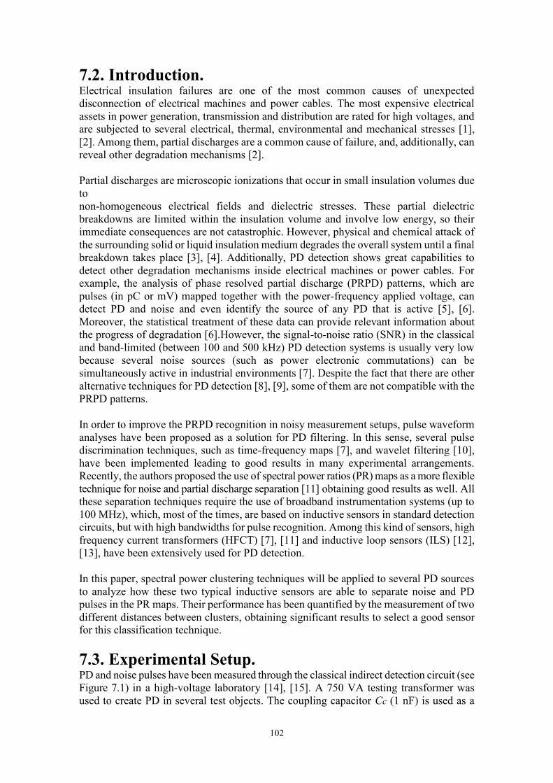
102

7.2. Introduction. Electrical insulation failures are one of the most common causes of unexpected disconnection of electrical machines and power cables. The most expensive electrical assets in power generation, transmission and distribution are rated for high voltages, and are subjected to several electrical, thermal, environmental and mechanical stresses [1], [2]. Among them, partial discharges are a common cause of failure, and, additionally, can reveal other degradation mechanisms [2]. Partial discharges are microscopic ionizations that occur in small insulation volumes due to non-homogeneous electrical fields and dielectric stresses. These partial dielectric breakdowns are limited within the insulation volume and involve low energy, so their immediate consequences are not catastrophic. However, physical and chemical attack of the surrounding solid or liquid insulation medium degrades the overall system until a final breakdown takes place [3], [4]. Additionally, PD detection shows great capabilities to detect other degradation mechanisms inside electrical machines or power cables. For example, the analysis of phase resolved partial discharge (PRPD) patterns, which are pulses (in pC or mV) mapped together with the power-frequency applied voltage, can detect PD and noise and even identify the source of any PD that is active [5], [6]. Moreover, the statistical treatment of these data can provide relevant information about the progress of degradation [6].However, the signal-to-noise ratio (SNR) in the classical and band-limited (between 100 and 500 kHz) PD detection systems is usually very low because several noise sources (such as power electronic commutations) can be simultaneously active in industrial environments [7]. Despite the fact that there are other alternative techniques for PD detection [8], [9], some of them are not compatible with the PRPD patterns. In order to improve the PRPD recognition in noisy measurement setups, pulse waveform analyses have been proposed as a solution for PD filtering. In this sense, several pulse discrimination techniques, such as time-frequency maps [7], and wavelet filtering [10], have been implemented leading to good results in many experimental arrangements. Recently, the authors proposed the use of spectral power ratios (PR) maps as a more flexible technique for noise and partial discharge separation [11] obtaining good results as well. All these separation techniques require the use of broadband instrumentation systems (up to 100 MHz), which, most of the times, are based on inductive sensors in standard detection circuits, but with high bandwidths for pulse recognition. Among this kind of sensors, high frequency current transformers (HFCT) [7], [11] and inductive loop sensors (ILS) [12], [13], have been extensively used for PD detection. In this paper, spectral power clustering techniques will be applied to several PD sources to analyze how these two typical inductive sensors are able to separate noise and PD pulses in the PR maps. Their performance has been quantified by the measurement of two different distances between clusters, obtaining significant results to select a good sensor for this classification technique. 7.3. Experimental Setup. PD and noise pulses have been measured through the classical indirect detection circuit (see Figure 7.1) in a high-voltage laboratory [14], [15]. A 750 VA testing transformer was used to create PD in several test objects. The coupling capacitor Cc (1 nF) is used as a

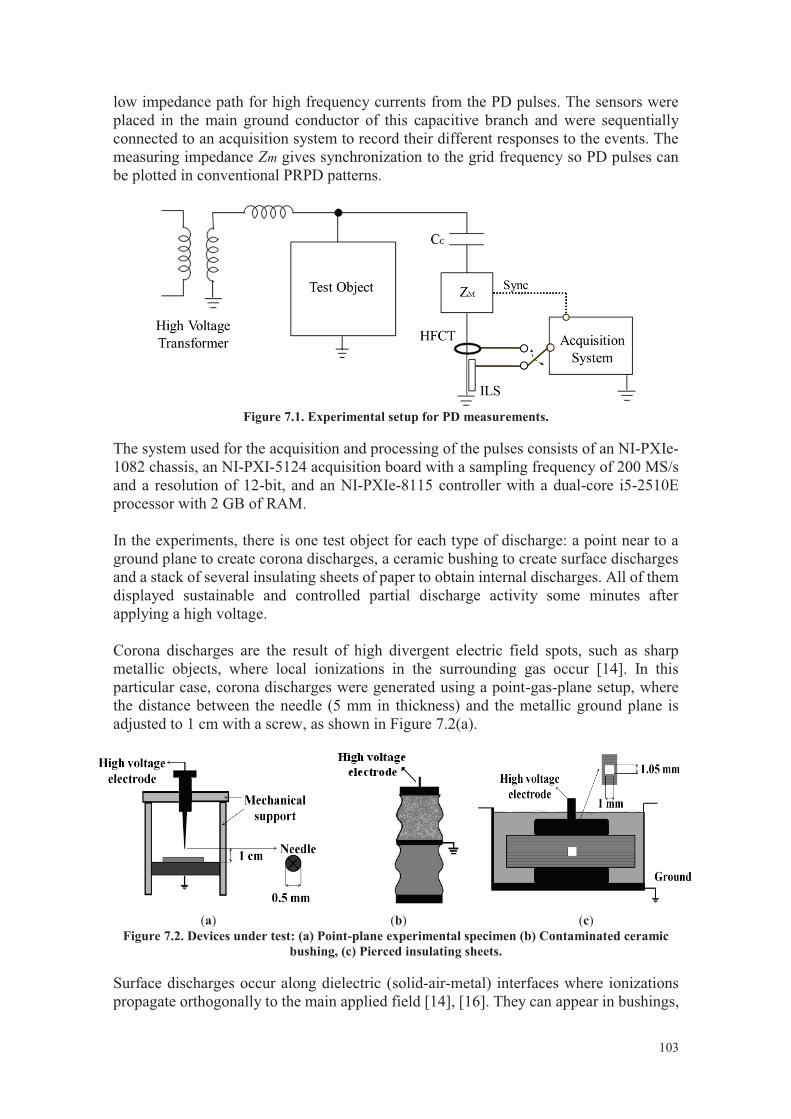
104

outdoor insulators and in electrical machine end-windings. In this experiment, high voltage was applied to one of the connections of a ceramic bushing, see Figure 7.2(b). Additionally, the insulator surface was contaminated with a saline solution, simulating a very common condition in coastal environments. A copper band was wrapped around and connected to ground in order to create shorter paths for surface discharges. Internal PD are discharges that occur inside small voids in non-homogeneous solid dielectrics, usually containing gas, due to the differences in permittivity and dielectric strength [14]. The setup to generate internal discharges consists of eleven insulating sheets of NOMEX paper (polyimide 0.35 mm thick film; typically used in high voltage generators as slot insulation systems). Three of the central papers were pierced with a needle, creating an air hole (1 mm in diameter) with a circular shape. The overall layered dielectric was wrapped with a plastic envelope to create vacuum inside and the whole system was immersed in mineral oil to avoid surface discharges at low voltages, guaranteeing the generation of internal PD within the cylindrical void at moderate voltage levels (see Figure 7.2(c)). For all test objects and with each sensor, noise, PD and the simultaneous acquisition of both phenomena are obtained following the procedure described in Table 7.1. The applied voltage is low when characterizing noise and high when acquiring PD. The differences in the applied voltage are determined by the partial discharge inception voltage (PDIV), which is different for each test object. The trigger level is low when capturing noise and high only when PD are acquired.

Table 7.1. Trigger and voltage levels to characterize noise, PD and PD + noise.

Characterization Applied Voltage Trigger Level Noise Low Low PD High High PD and noise High Low

To obtain statistically significant results in each experiment, 1,000 pulses were acquired with one source (PD or noise) and 3,000 pulses were acquired when two simultaneous sources were active (PD and noise). This procedure guarantees the reliability of the observed phenomenon, since PD are ionization processes governed by the laws of statistical mechanics [3], [4]. The procedure was repeated individually for each sensor, because their sensitivity is different (see Section 7.4) and the acquisition system only has two channels (one for the sensor and another for the synchronization signal) so the simultaneous acquisition of the same pulses with the two sensors is impossible with this setup. 7.4. Inductive Sensors for PD Detection. Inductive sensors are common measuring devices for rapidly varying currents, such as partial discharges [17]. In this paper, a high-frequency current transformer and an inductive loop will be validated for the proposed spectral power ratios separation technique (explained in Section 7.5), see Figure 7.3.

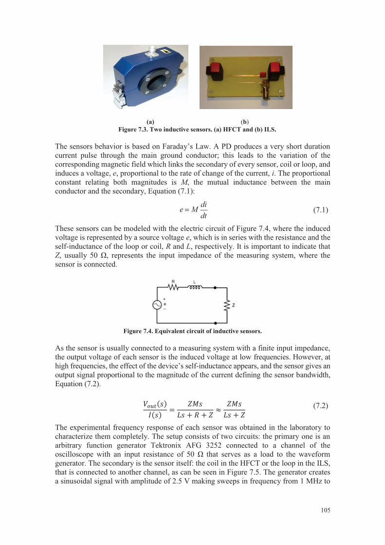
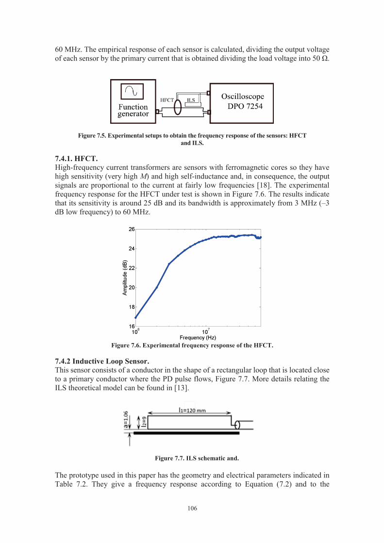
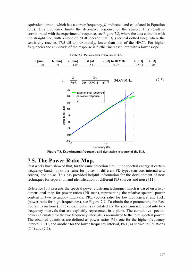
107

equivalent circuit, which has a corner frequency, fc, indicated and calculated in Equation (7.3). This frequency limits the derivative response of the sensor. This result is corroborated with the experimental response, see Figure 7.8, where the data coincide with the straight line, with a slope of 20 dB/decade, until fc, (vertical dotted line), where the sensitivity reaches 17.5 dB approximately, lower than that of the HFCT. For higher frequencies the amplitude of the response is further increased, but with a lower slope.

Table 7.2. Parameters of the used ILS.

l1 [mm] l2 [mm] a [mm] M [nH] R [Ω] to 10 MHz L [nH] Z [Ω] 120 9 1.06 54.9 0.22 229.4 50

𝑓𝑐 =𝑍

2𝜋𝐿=

50

2𝜋 ∙ 229.4 ∙ 10−9= 34.69 MHz (7.3)

Figure 7.8. Experimental frequency and derivative response of the ILS.

7.5. The Power Ratio Map. Past works have showed that, for the same detection circuit, the spectral energy at certain frequency bands is not the same for pulses of different PD types (surface, internal and corona) and noise. This has provided helpful information for the development of new techniques for separation and identification of different PD sources and noise [11]. Reference [11] presents the spectral power clustering technique, which is based on a two-dimensional map for power ratios (PR map), representing the relative spectral power content in two frequency intervals: PRL (power ratio for low frequencies) and PRH (power ratio for high frequencies), see Figure 7.9. To obtain these parameters, the Fast Fourier Transform (FFT) of each pulse is calculated and the spectrum is divided into two frequency intervals that are explicitly represented in a plane. The cumulative spectral power calculated for the two frequency intervals is normalized to the total spectral power. The obtained quantities are defined as power ratios (%), one for the higher frequency interval, PRH, and another for the lower frequency interval, PRL, as shown in Equations (7.4) and (7.5).

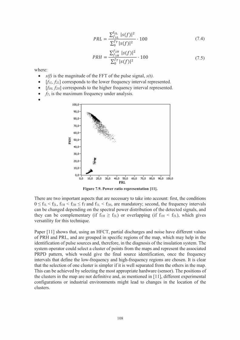
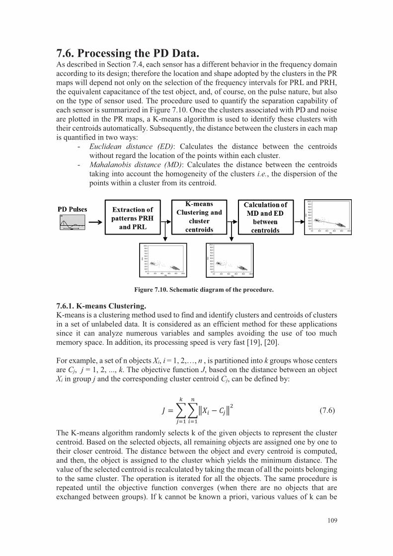
110

evaluated until the most suitable one is found. The effectiveness of this method, as well as of others, relies heavily on the objective function used in measuring the distance between objects [21], [22]. Concretely, the steps of the k-means algorithm can be summarized in:

1. Initialize the clusters centroids. 2. Group each data point into the nearest cluster based on distance calculation. 3. Recalculate each center using the mean of all the points in the same cluster. 4. Move some data points from one cluster to another to make J smaller, and

return to step 2 until the convergence condition is met.

7.6.2. Euclidean Distance. The most widely used distance is the ED. It is simple computationally, but this parameter does not consider the structure of the data [23], [24]. The Euclidean distance between any two clusters of data, A and B, is the distance between their centroids and is given by:

𝐸𝐷2 = (C𝐴 − C𝐵)T(C𝐴 − C𝐵) (7.7) where, CA and CB are centroids of the clusters A and B. In this particular case, (CA − CB) is a vector, since the representation of the points is done in two dimensions (PR maps). 7.6.3. Mahalanobis Distance. The ED is often invalid and generally undesirable in many practical applications since it ignores helpful parameters about the data, such as homogeneity or dispersion. Thus, the MD is better in this aspect because it includes the variances of the data as weights to modify the distance [23], [25]. The MD between two clusters of data, A and B, is given by:

𝑀𝐷2 = (C𝐴 − C𝐵)T(𝑉𝐴−1 − 𝑉𝐵

−1)(C𝐴 − C𝐵) (7.8)

where, VA and VB represent the covariance matrices computed from of A and B, Equations (7.9) and (7.10).

𝑉𝐴 =1

NA∗ ∑(𝐴𝑗 − C𝐴)

T(𝐴𝑗 − C𝐴)

NA

𝑗=1

(7.9)

𝑉𝐵 =1

NB∗ ∑(𝐵𝑗 − C𝐵)

T(𝐵𝑗 − C𝐵)

NB

𝑗=1

(7.10)

where, NA and NB are number of data within each cluster. 7.7. Experimental Results. This section presents the results quantifying the separation capability between clusters associated with PD sources and noise. These are obtained by applying the spectral power clustering technique to the signals measured in different test objects with the HFCT and ILS sensors. The PR maps and the normalized average spectral power (it is has been normalized in such a way that the maximum spectral peak is equal to 1) of the pulses captured by two sensors are described in all the test objects. Due to the fact that the HFCT

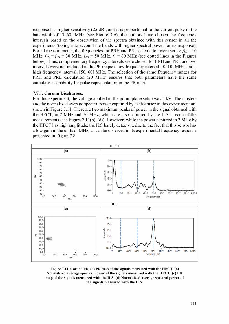
111

response has higher sensitivity (25 dB), and it is proportional to the current pulse in the bandwidth of [3–60] MHz (see Figure 7.6), the authors have chosen the frequency intervals based on the observation of the spectra obtained with this sensor in all the experiments (taking into account the bands with higher spectral power for its response). For all measurements, the frequencies for PRH and PRL calculation were set to: f1L = 10 MHz, f2L = f1H = 30 MHz, f2H = 50 MHz, fT = 60 MHz (see dotted lines in the Figures below). Thus, complementary frequency intervals were chosen for PRH and PRL and two intervals were not included in the PR maps: a low frequency interval, [0, 10] MHz, and a high frequency interval, [50, 60] MHz. The selection of the same frequency ranges for PRH and PRL calculation (20 MHz) ensures that both parameters have the same cumulative capability for pulse representation in the PR map. 7.7.1. Corona Discharges. For this experiment, the voltage applied to the point–plane setup was 5 kV. The clusters and the normalized average spectral power captured by each sensor in this experiment are shown in Figure 7.11. There are two maximum peaks of power in the signal obtained with the HFCT, in 2 MHz and 50 MHz, which are also captured by the ILS in each of the measurements (see Figure 7.11(b), (d)). However, while the power captured in 2 MHz by the HFCT has high amplitude, the ILS barely detects it, due to the fact that this sensor has a low gain in the units of MHz, as can be observed in its experimental frequency response presented in Figure 7.8.

HFCT (a) (b)

ILS

(c) (d)

Figure 7.11. Corona PD. (a) PR map of the signals measured with the HFCT, (b) Normalized average spectral power of the signals measured with the HFCT, (c) PR

map of the signals measured with the ILS, (d) Normalized average spectral power of the signals measured with the ILS.

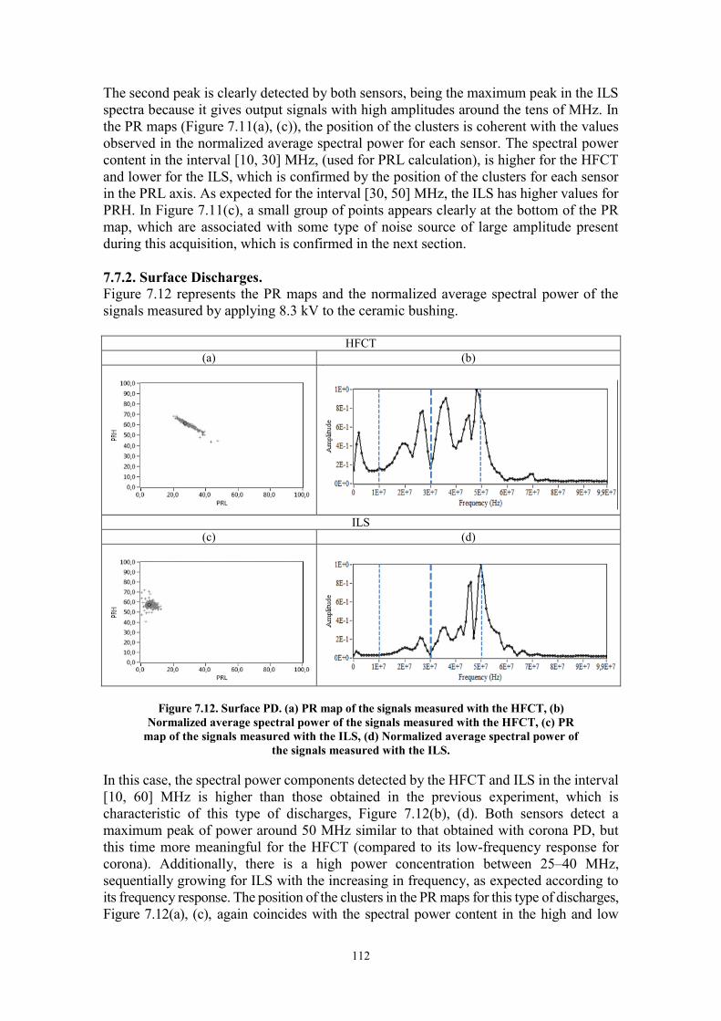
112

The second peak is clearly detected by both sensors, being the maximum peak in the ILS spectra because it gives output signals with high amplitudes around the tens of MHz. In the PR maps (Figure 7.11(a), (c)), the position of the clusters is coherent with the values observed in the normalized average spectral power for each sensor. The spectral power content in the interval [10, 30] MHz, (used for PRL calculation), is higher for the HFCT and lower for the ILS, which is confirmed by the position of the clusters for each sensor in the PRL axis. As expected for the interval [30, 50] MHz, the ILS has higher values for PRH. In Figure 7.11(c), a small group of points appears clearly at the bottom of the PR map, which are associated with some type of noise source of large amplitude present during this acquisition, which is confirmed in the next section.

7.7.2. Surface Discharges. Figure 7.12 represents the PR maps and the normalized average spectral power of the signals measured by applying 8.3 kV to the ceramic bushing.

HFCT (a) (b)

v

ILS

(c) (d)

Figure 7.12. Surface PD. (a) PR map of the signals measured with the HFCT, (b) Normalized average spectral power of the signals measured with the HFCT, (c) PR

map of the signals measured with the ILS, (d) Normalized average spectral power of the signals measured with the ILS.

In this case, the spectral power components detected by the HFCT and ILS in the interval [10, 60] MHz is higher than those obtained in the previous experiment, which is characteristic of this type of discharges, Figure 7.12(b), (d). Both sensors detect a maximum peak of power around 50 MHz similar to that obtained with corona PD, but this time more meaningful for the HFCT (compared to its low-frequency response for corona). Additionally, there is a high power concentration between 25–40 MHz, sequentially growing for ILS with the increasing in frequency, as expected according to its frequency response. The position of the clusters in the PR maps for this type of discharges, Figure 7.12(a), (c), again coincides with the spectral power content in the high and low

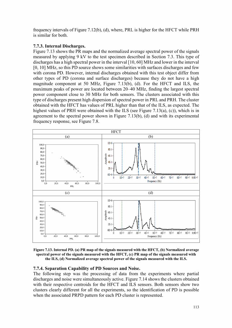
113

frequency intervals of Figure 7.12(b), (d), where, PRL is higher for the HFCT while PRH is similar for both. 7.7.3. Internal Discharges. Figure 7.13 shows the PR maps and the normalized average spectral power of the signals measured by applying 9 kV to the test specimen described in Section 7.3. This type of discharges has a high spectral power in the interval [10, 60] MHz and lower in the interval [0, 10] MHz, so this PD source shows some similarities with surfaces discharges and few with corona PD. However, internal discharges obtained with this test object differ from other types of PD (corona and surface discharges) because they do not have a high magnitude component at 50 MHz, Figure 7.13(b), (d). For the HFCT and ILS, the maximum peaks of power are located between 20–40 MHz, finding the largest spectral power component close to 30 MHz for both sensors. The clusters associated with this type of discharges present high dispersion of spectral power in PRL and PRH. The cluster obtained with the HFCT has values of PRL higher than that of the ILS, as expected. The highest values of PRH were obtained with the ILS (see Figure 7.13(a), (c)), which is in agreement to the spectral power shown in Figure 7.13(b), (d) and with its experimental frequency response, see Figure 7.8.

HFCT (a) (b)

(c) (d)

Figure 7.13. Internal PD. (a) PR map of the signals measured with the HFCT, (b) Normalized average spectral power of the signals measured with the HFCT, (c) PR map of the signals measured with

the ILS, (d) Normalized average spectral power of the signals measured with the ILS.

7.7.4. Separation Capability of PD Sources and Noise. The following step was the processing of data from the experiments where partial discharges and noise were simultaneously active. Figure 7.14 shows the clusters obtained with their respective centroids for the HFCT and ILS sensors. Both sensors show two clusters clearly different for all the experiments, so the identification of PD is possible when the associated PRPD pattern for each PD cluster is represented.

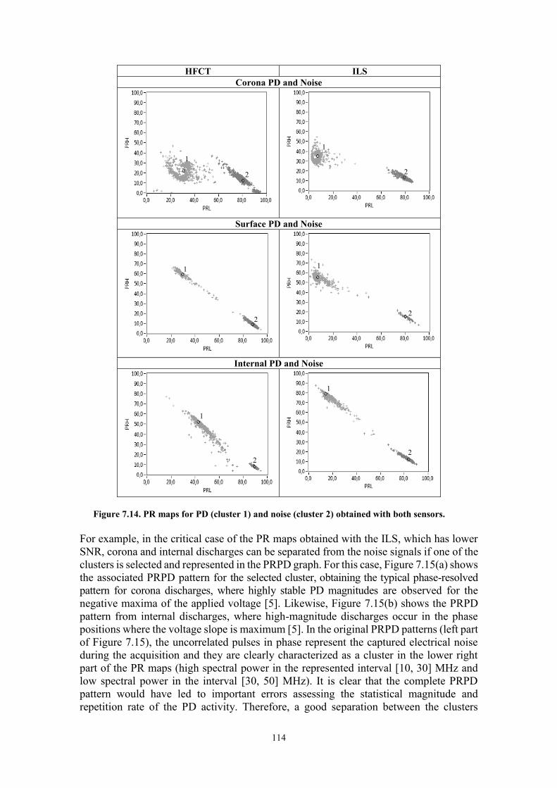
114

HFCT ILS Corona PD and Noise

Surface PD and Noise

Internal PD and Noise

Figure 7.14. PR maps for PD (cluster 1) and noise (cluster 2) obtained with both sensors. For example, in the critical case of the PR maps obtained with the ILS, which has lower SNR, corona and internal discharges can be separated from the noise signals if one of the clusters is selected and represented in the PRPD graph. For this case, Figure 7.15(a) shows the associated PRPD pattern for the selected cluster, obtaining the typical phase-resolved pattern for corona discharges, where highly stable PD magnitudes are observed for the negative maxima of the applied voltage [5]. Likewise, Figure 7.15(b) shows the PRPD pattern from internal discharges, where high-magnitude discharges occur in the phase positions where the voltage slope is maximum [5]. In the original PRPD patterns (left part of Figure 7.15), the uncorrelated pulses in phase represent the captured electrical noise during the acquisition and they are clearly characterized as a cluster in the lower right part of the PR maps (high spectral power in the represented interval [10, 30] MHz and low spectral power in the interval [30, 50] MHz). It is clear that the complete PRPD pattern would have led to important errors assessing the statistical magnitude and repetition rate of the PD activity. Therefore, a good separation between the clusters

1

2

1

2

1

2

1

2

1

2

1

2

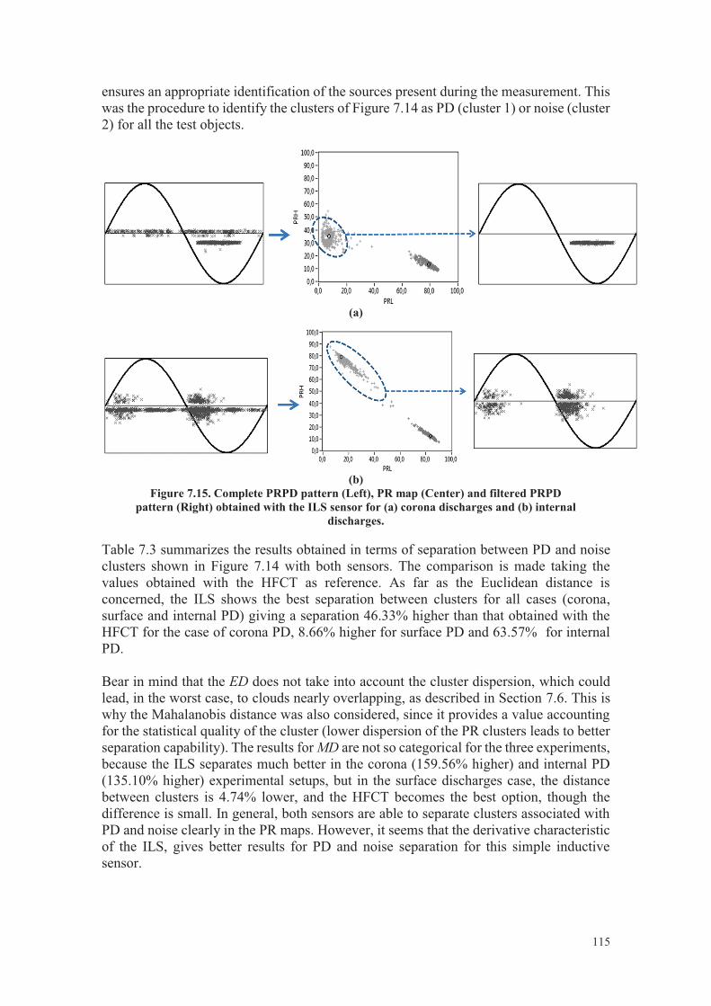
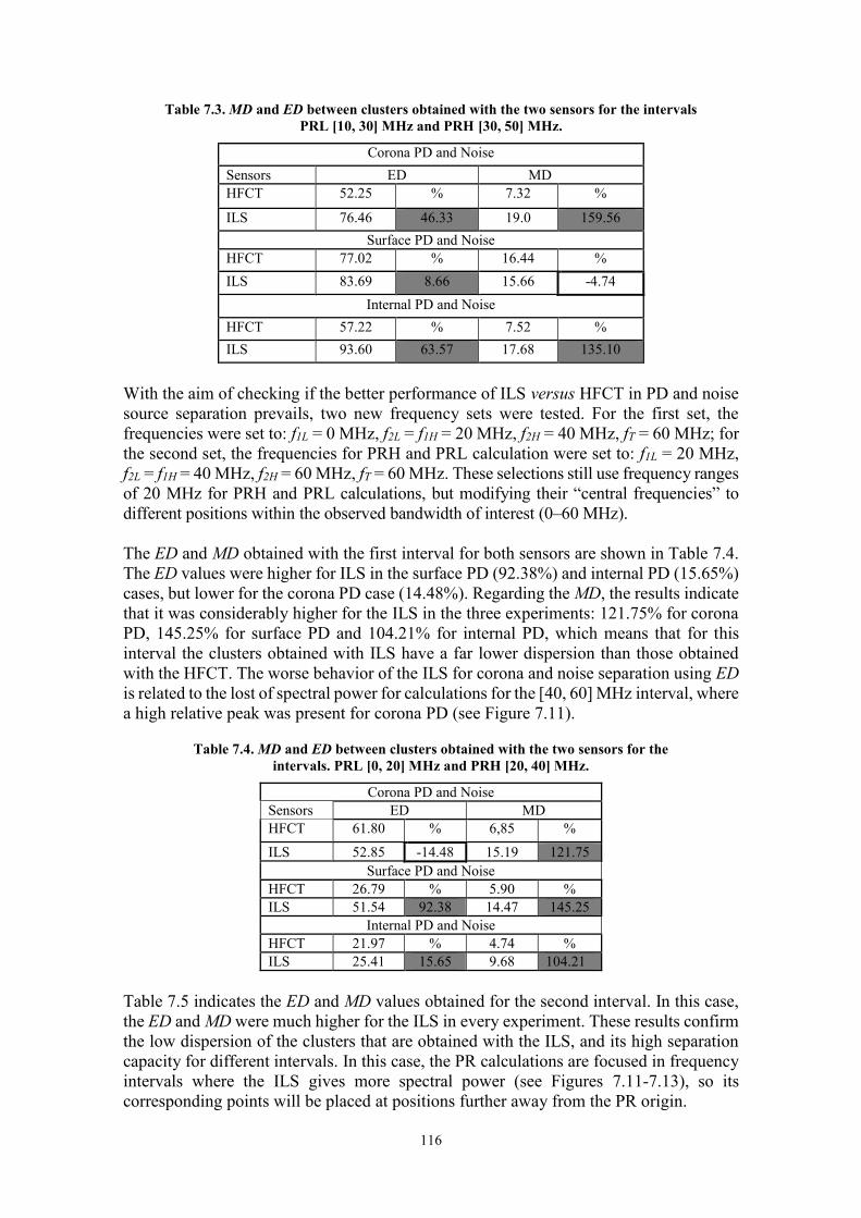
116

Table 7.3. MD and ED between clusters obtained with the two sensors for the intervals PRL [10, 30] MHz and PRH [30, 50] MHz.

Corona PD and Noise Sensors ED MD HFCT 52.25 % 7.32 %

ILS 76.46 46.33 19.0 159.56 Surface PD and Noise

HFCT 77.02 % 16.44 % ILS 83.69 8.66 15.66 -4.74

Internal PD and Noise HFCT 57.22 % 7.52 % ILS 93.60 63.57 17.68 135.10

With the aim of checking if the better performance of ILS versus HFCT in PD and noise source separation prevails, two new frequency sets were tested. For the first set, the frequencies were set to: f1L = 0 MHz, f2L = f1H = 20 MHz, f2H = 40 MHz, fT = 60 MHz; for the second set, the frequencies for PRH and PRL calculation were set to: f1L = 20 MHz, f2L = f1H = 40 MHz, f2H = 60 MHz, fT = 60 MHz. These selections still use frequency ranges of 20 MHz for PRH and PRL calculations, but modifying their “central frequencies” to different positions within the observed bandwidth of interest (0–60 MHz). The ED and MD obtained with the first interval for both sensors are shown in Table 7.4. The ED values were higher for ILS in the surface PD (92.38%) and internal PD (15.65%) cases, but lower for the corona PD case (14.48%). Regarding the MD, the results indicate that it was considerably higher for the ILS in the three experiments: 121.75% for corona PD, 145.25% for surface PD and 104.21% for internal PD, which means that for this interval the clusters obtained with ILS have a far lower dispersion than those obtained with the HFCT. The worse behavior of the ILS for corona and noise separation using ED is related to the lost of spectral power for calculations for the [40, 60] MHz interval, where a high relative peak was present for corona PD (see Figure 7.11).

Table 7.4. MD and ED between clusters obtained with the two sensors for the intervals. PRL [0, 20] MHz and PRH [20, 40] MHz.

Corona PD and Noise Sensors ED MD HFCT 61.80 % 6,85 %

ILS 52.85 -14.48 15.19 121.75 Surface PD and Noise

HFCT 26.79 % 5.90 % ILS 51.54 92.38 14.47 145.25


Table 7.5 indicates the ED and MD values obtained for the second interval. In this case, the ED and MD were much higher for the ILS in every experiment. These results confirm the low dispersion of the clusters that are obtained with the ILS, and its high separation capacity for different intervals. In this case, the PR calculations are focused in frequency intervals where the ILS gives more spectral power (see Figures 7.11-7.13), so its corresponding points will be placed at positions further away from the PR origin.

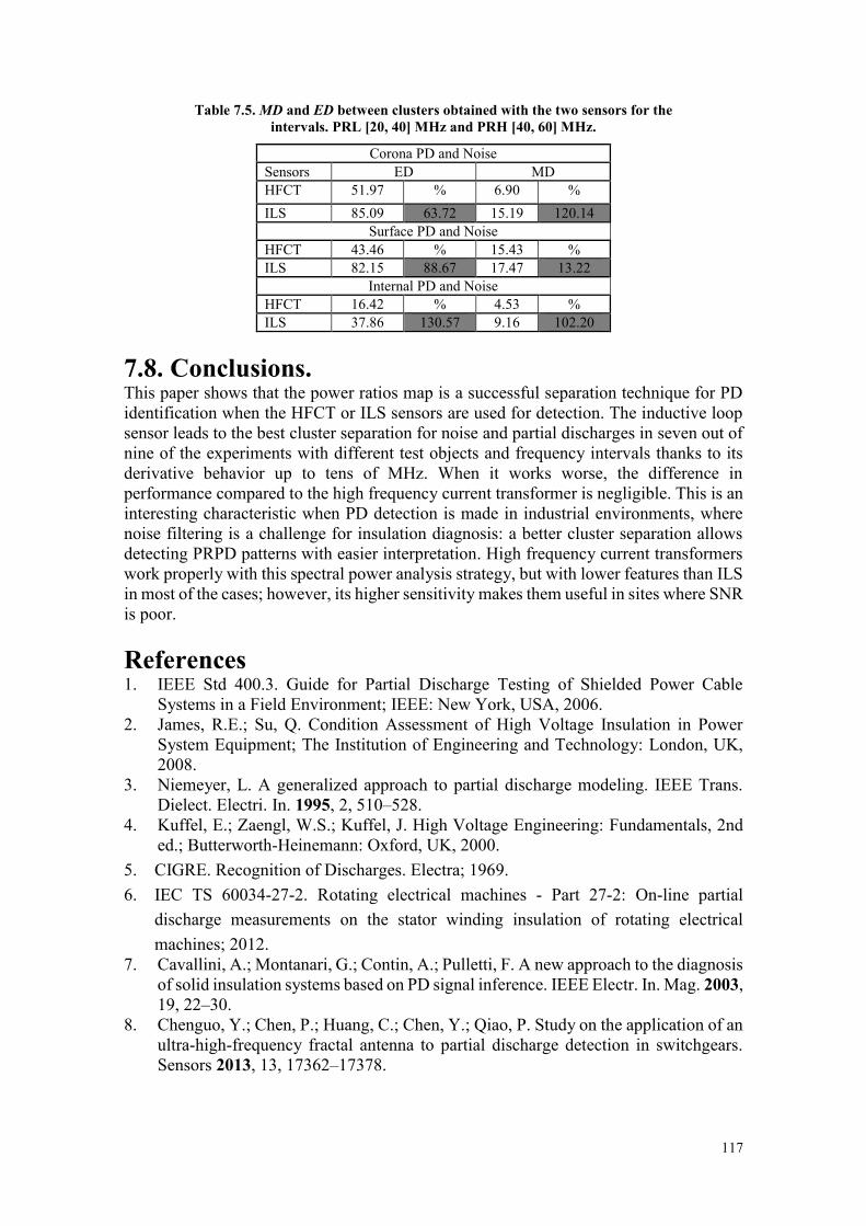
117

Table 7.5. MD and ED between clusters obtained with the two sensors for the intervals. PRL [20, 40] MHz and PRH [40, 60] MHz.

Corona PD and Noise Sensors ED MD HFCT 51.97 % 6.90 % ILS 85.09 63.72 15.19 120.14

Surface PD and Noise HFCT 43.46 % 15.43 % ILS 82.15 88.67 17.47 13.22


7.8. Conclusions. This paper shows that the power ratios map is a successful separation technique for PD identification when the HFCT or ILS sensors are used for detection. The inductive loop sensor leads to the best cluster separation for noise and partial discharges in seven out of nine of the experiments with different test objects and frequency intervals thanks to its derivative behavior up to tens of MHz. When it works worse, the difference in performance compared to the high frequency current transformer is negligible. This is an interesting characteristic when PD detection is made in industrial environments, where noise filtering is a challenge for insulation diagnosis: a better cluster separation allows detecting PRPD patterns with easier interpretation. High frequency current transformers work properly with this spectral power analysis strategy, but with lower features than ILS in most of the cases; however, its higher sensitivity makes them useful in sites where SNR is poor. References 1. IEEE Std 400.3. Guide for Partial Discharge Testing of Shielded Power Cable

Systems in a Field Environment; IEEE: New York, USA, 2006. 2. James, R.E.; Su, Q. Condition Assessment of High Voltage Insulation in Power

System Equipment; The Institution of Engineering and Technology: London, UK, 2008.

3. Niemeyer, L. A generalized approach to partial discharge modeling. IEEE Trans. Dielect. Electri. In. 1995, 2, 510–528.

4. Kuffel, E.; Zaengl, W.S.; Kuffel, J. High Voltage Engineering: Fundamentals, 2nd ed.; Butterworth-Heinemann: Oxford, UK, 2000.

5. CIGRE. Recognition of Discharges. Electra; 1969. 6. IEC TS 60034-27-2. Rotating electrical machines - Part 27-2: On-line partial

discharge measurements on the stator winding insulation of rotating electrical machines; 2012.

7. Cavallini, A.; Montanari, G.; Contin, A.; Pulletti, F. A new approach to the diagnosis of solid insulation systems based on PD signal inference. IEEE Electr. In. Mag. 2003, 19, 22–30.

8. Chenguo, Y.; Chen, P.; Huang, C.; Chen, Y.; Qiao, P. Study on the application of an ultra-high-frequency fractal antenna to partial discharge detection in switchgears. Sensors 2013, 13, 17362–17378.

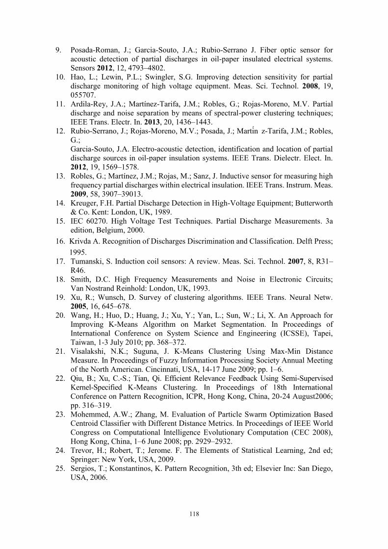
118

9. Posada-Roman, J.; Garcia-Souto, J.A.; Rubio-Serrano J. Fiber optic sensor for acoustic detection of partial discharges in oil-paper insulated electrical systems. Sensors 2012, 12, 4793–4802.

10. Hao, L.; Lewin, P.L.; Swingler, S.G. Improving detection sensitivity for partial discharge monitoring of high voltage equipment. Meas. Sci. Technol. 2008, 19, 055707.

11. Ardila-Rey, J.A.; Martínez-Tarifa, J.M.; Robles, G.; Rojas-Moreno, M.V. Partial discharge and noise separation by means of spectral-power clustering techniques; IEEE Trans. Electr. In. 2013, 20, 1436–1443.

12. Rubio-Serrano, J.; Rojas-Moreno, M.V.; Posada, J.; Martin z-Tarifa, J.M.; Robles, G.; Garcia-Souto, J.A. Electro-acoustic detection, identification and location of partial discharge sources in oil-paper insulation systems. IEEE Trans. Dielectr. Elect. In. 2012, 19, 1569–1578.

13. Robles, G.; Martínez, J.M.; Rojas, M.; Sanz, J. Inductive sensor for measuring high frequency partial discharges within electrical insulation. IEEE Trans. Instrum. Meas. 2009, 58, 3907–39013.

14. Kreuger, F.H. Partial Discharge Detection in High-Voltage Equipment; Butterworth & Co. Kent: London, UK, 1989.

15. IEC 60270. High Voltage Test Techniques. Partial Discharge Measurements. 3a edition, Belgium, 2000.

16. Krivda A. Recognition of Discharges Discrimination and Classification. Delft Press; 1995.

17. Tumanski, S. Induction coil sensors: A review. Meas. Sci. Technol. 2007, 8, R31–R46.

18. Smith, D.C. High Frequency Measurements and Noise in Electronic Circuits; Van Nostrand Reinhold: London, UK, 1993.

19. Xu, R.; Wunsch, D. Survey of clustering algorithms. IEEE Trans. Neural Netw. 2005, 16, 645–678.

20. Wang, H.; Huo, D.; Huang, J.; Xu, Y.; Yan, L.; Sun, W.; Li, X. An Approach for Improving K-Means Algorithm on Market Segmentation. In Proceedings of International Conference on System Science and Engineering (ICSSE), Tapei, Taiwan, 1-3 July 2010; pp. 368–372.

21. Visalakshi, N.K.; Suguna, J. K-Means Clustering Using Max-Min Distance Measure. In Proceedings of Fuzzy Information Processing Society Annual Meeting of the North American. Cincinnati, USA, 14-17 June 2009; pp. 1–6.

22. Qiu, B.; Xu, C.-S.; Tian, Qi. Efficient Relevance Feedback Using Semi-Supervised Kernel-Specified K-Means Clustering. In Proceedings of 18th International Conference on Pattern Recognition, ICPR, Hong Kong, China, 20-24 August2006; pp. 316–319.

23. Mohemmed, A.W.; Zhang, M. Evaluation of Particle Swarm Optimization Based Centroid Classifier with Different Distance Metrics. In Proceedings of IEEE World Congress on Computational Intelligence Evolutionary Computation (CEC 2008), Hong Kong, China, 1–6 June 2008; pp. 2929–2932.

24. Trevor, H.; Robert, T.; Jerome. F. The Elements of Statistical Learning, 2nd ed; Springer: New York, USA, 2009.

25. Sergios, T.; Konstantinos, K. Pattern Recognition, 3th ed; Elsevier Inc: San Diego, USA, 2006.

119

Chapter 8

Automatic selection of frequency bands for the power ratios separation technique

in partial discharge measurements Contents 8.1. Abstract ................................................................................................................. 119 8.2. Introduction ........................................................................................................... 120 8.3. The power ratios as a separation technique ........................................................... 121 8.4. Quantification of the PR maps separation capability ............................................ 122 8.5. The strategy for frequency selection ..................................................................... 123 8.6. Experimental setup ................................................................................................ 126 8.7. Results for PD and noise separation in simple test objects ................................... 127 8.7.1. Review of previous results using user-selected intervals ................................. 127 8.7.2. Automatic selection of frequency intervals ...................................................... 128 8.7.2.1. Corona discharges and noise ....................................................................... 129 8.7.2.2. Internal discharges and noise ....................................................................... 131 8.7.2.3. Surface discharges and noise ....................................................................... 133

8.8. Results for PD source separation ........................................................................... 134 8.8.1. Internal and corona discharges ......................................................................... 134 8.8.2. Internal and surface discharges ......................................................................... 137

8.9. Application in an insulated power cable................................................................ 140 8.9.1. PD and noise detection in the cable .................................................................. 140 8.9.2. Separation of simultaneous discharges from the power cable and corona source .................................................................................................................................... 141

8.10. Discussion ............................................................................................................ 143 References .................................................................................................................... 144

8.1. Abstract. Partial discharge (PD) measurements are important for the monitoring of the status of almost any type of high-voltage equipment. The use of this technique for on-line measurements involves several challenges related to noise rejection and PD source recognition. In order to face these issues, pulse shape analyses are made in high-frequency and very-high-frequency ranges. The authors proposed in a previous paper the so-called Power Ratios (PR) of the spectra as useful parameters for pulse source separation in a two-dimensional approach. This technique provides good results, but its reliability depends on the appropriate selection of two frequency intervals where these spectral power ratios are calculated. In order to improve this separation system, the authors propose an algorithm that provides very good separation results in several experimental setups. The simultaneous measurements of pulse sources (PD or noise) are complemented

120

with pulse characterization when only one single source is active in order to check that the selected frequency intervals are appropriate. In addition to simple test objects to create typical PD sources (corona, internal and surface), the authors show results for tests on two power cables. 8.2. Introduction. It is a well-known fact that electrical machines and power cables rated for high voltages show unexpected failures even when their rated stresses (thermal, mechanical, electrical…) are not exceeded [1], [2]. In order to prevent these failures, condition monitoring is a current topic of great interest for utilities and the users of these expensive assets [3], [4], [5]. Among several measurement techniques, partial discharge (PD) characterization seems to be one of the most versatile choices for several reasons [2], [6], [7]: it can be applied to any high voltage asset, it can be used on-line, and it can detect many degradation mechanisms. There is much information to detect many insulation defects by means of the magnitude-phase representation of PD signals in what is called Phase Resolved Partial Discharge (PRPD) patterns [7], [8], [9]. However, the tendency of using this technique in on-line applications leads to great problems to identify one PD source when the noise level is very high. In addition, it is quite common that several PD sources might be simultaneously active, so the PRPD recognition becomes impossible. Thus, pulse waveforms have been analyzed in several ways with the aim of separating several simultaneous pulse sources [10], [11], [12], so the selection of one type of pulse source can be made (usually in two or three dimensional maps) to identify its associated PRPD pattern. Following this research trend, the authors proposed in a previous paper another technique for pulse source separation [13], based in the so-called Power Ratios (PR). In this approach, each pulse is analyzed in the frequency domain, calculating its spectral power in two characteristic frequency intervals divided into their total spectral power. These two parameters were represented in a two dimensional map, where each pulse source showed a different cloud of points (clusters) with different positions. This separation technique shows great results for all the experiments made up to this time focused not only on PD-noise separation, but also on PD source identification [13], [14], [15]. One essential characteristic of this technique is its flexibility, since changing the analyzed frequency intervals can improve the cluster separation if the initially set up frequency intervals were not appropriate [14]. However, in some cases, the choice of these intervals can be tricky because the signals could have similar power spectra or the operator may not be experienced in selecting them. Under these circumstances it is important to provide an automated selection of intervals that give a good separation of noise and PD clusters in a PR map. In this paper, an algorithm for the automatic selection of the frequency intervals that increase the separation between clusters represented in a PR map is presented. It is based on the statistical dispersion of the share of power in different bands of frequency from experiments where simultaneous pulse sources are active. The distance between clusters to detect the appropriate selection was compared to previous experiments where several fixed intervals were used. The proposed technique is proven in several test objects

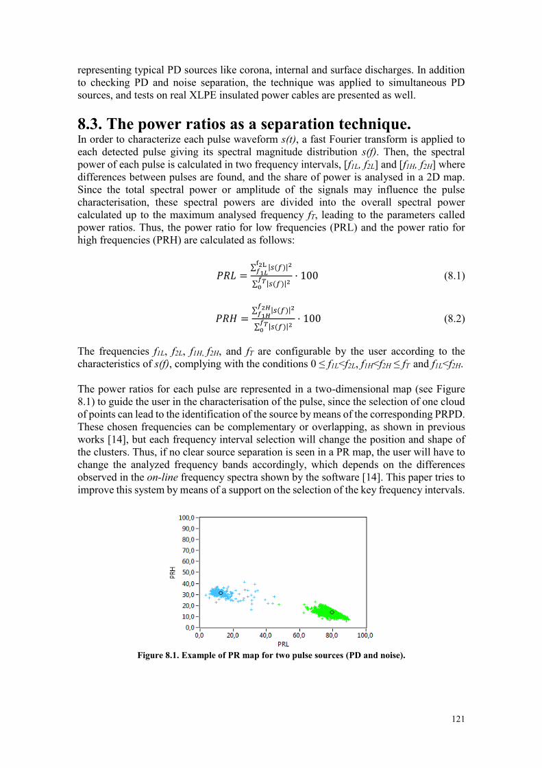
121

representing typical PD sources like corona, internal and surface discharges. In addition to checking PD and noise separation, the technique was applied to simultaneous PD sources, and tests on real XLPE insulated power cables are presented as well. 8.3. The power ratios as a separation technique. In order to characterize each pulse waveform s(t), a fast Fourier transform is applied to each detected pulse giving its spectral magnitude distribution s(f). Then, the spectral power of each pulse is calculated in two frequency intervals, [f1L, f2L] and [f1H, f2H] where differences between pulses are found, and the share of power is analysed in a 2D map. Since the total spectral power or amplitude of the signals may influence the pulse characterisation, these spectral powers are divided into the overall spectral power calculated up to the maximum analysed frequency fT, leading to the parameters called power ratios. Thus, the power ratio for low frequencies (PRL) and the power ratio for high frequencies (PRH) are calculated as follows:

𝑃𝑅𝐿 =∑ |𝑠(𝑓)|2f2L

𝑓1𝐿

∑ |𝑠(𝑓)|2𝑓𝑇0

· 100 (8.1)


𝑓1𝐻

∑ |𝑠(𝑓)|2𝑓𝑇0

· 100 (8.2)

The frequencies f1L, f2L, f1H, f2H, and fT are configurable by the user according to the characteristics of s(f), complying with the conditions 0 ≤ f1L<f2L, f1H<f2H ≤ fT and f1L<f2H. The power ratios for each pulse are represented in a two-dimensional map (see Figure 8.1) to guide the user in the characterisation of the pulse, since the selection of one cloud of points can lead to the identification of the source by means of the corresponding PRPD. These chosen frequencies can be complementary or overlapping, as shown in previous works [14], but each frequency interval selection will change the position and shape of the clusters. Thus, if no clear source separation is seen in a PR map, the user will have to change the analyzed frequency bands accordingly, which depends on the differences observed in the on-line frequency spectra shown by the software [14]. This paper tries to improve this system by means of a support on the selection of the key frequency intervals.

Figure 8.1. Example of PR map for two pulse sources (PD and noise).

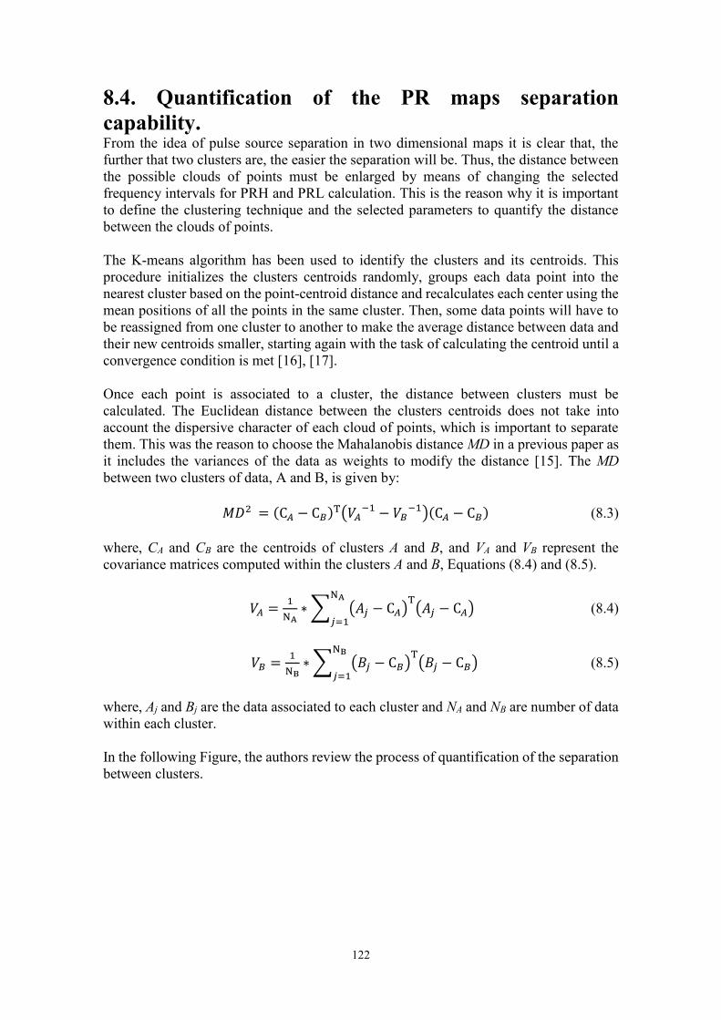
122

8.4. Quantification of the PR maps separation capability. From the idea of pulse source separation in two dimensional maps it is clear that, the further that two clusters are, the easier the separation will be. Thus, the distance between the possible clouds of points must be enlarged by means of changing the selected frequency intervals for PRH and PRL calculation. This is the reason why it is important to define the clustering technique and the selected parameters to quantify the distance between the clouds of points. The K-means algorithm has been used to identify the clusters and its centroids. This procedure initializes the clusters centroids randomly, groups each data point into the nearest cluster based on the point-centroid distance and recalculates each center using the mean positions of all the points in the same cluster. Then, some data points will have to be reassigned from one cluster to another to make the average distance between data and their new centroids smaller, starting again with the task of calculating the centroid until a convergence condition is met [16], [17]. Once each point is associated to a cluster, the distance between clusters must be calculated. The Euclidean distance between the clusters centroids does not take into account the dispersive character of each cloud of points, which is important to separate them. This was the reason to choose the Mahalanobis distance MD in a previous paper as it includes the variances of the data as weights to modify the distance [15]. The MD between two clusters of data, A and B, is given by:

𝑀𝐷2 = (C𝐴 − C𝐵)T(𝑉𝐴−1 − 𝑉𝐵

−1)(C𝐴 − C𝐵) (8.3) where, CA and CB are the centroids of clusters A and B, and VA and VB represent the covariance matrices computed within the clusters A and B, Equations (8.4) and (8.5).

𝑉𝐴 =1

NA∗ ∑ (𝐴𝑗 − C𝐴)

T(𝐴𝑗 − C𝐴)

NA

𝑗=1 (8.4)

𝑉𝐵 =1

NB∗ ∑ (𝐵𝑗 − C𝐵)

T(𝐵𝑗 − C𝐵)

NB

𝑗=1 (8.5)

where, Aj and Bj are the data associated to each cluster and NA and NB are number of data within each cluster. In the following Figure, the authors review the process of quantification of the separation between clusters.

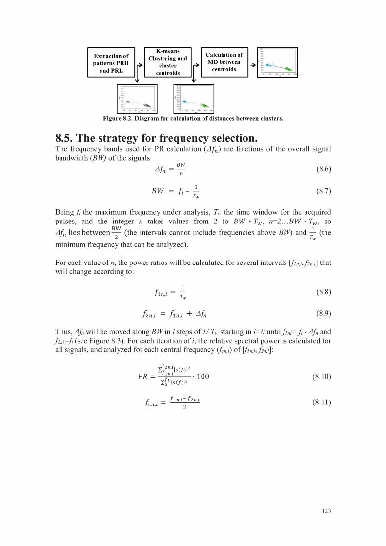
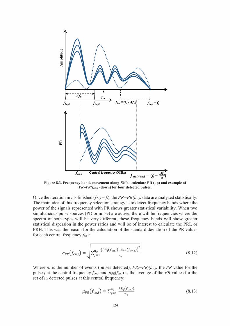
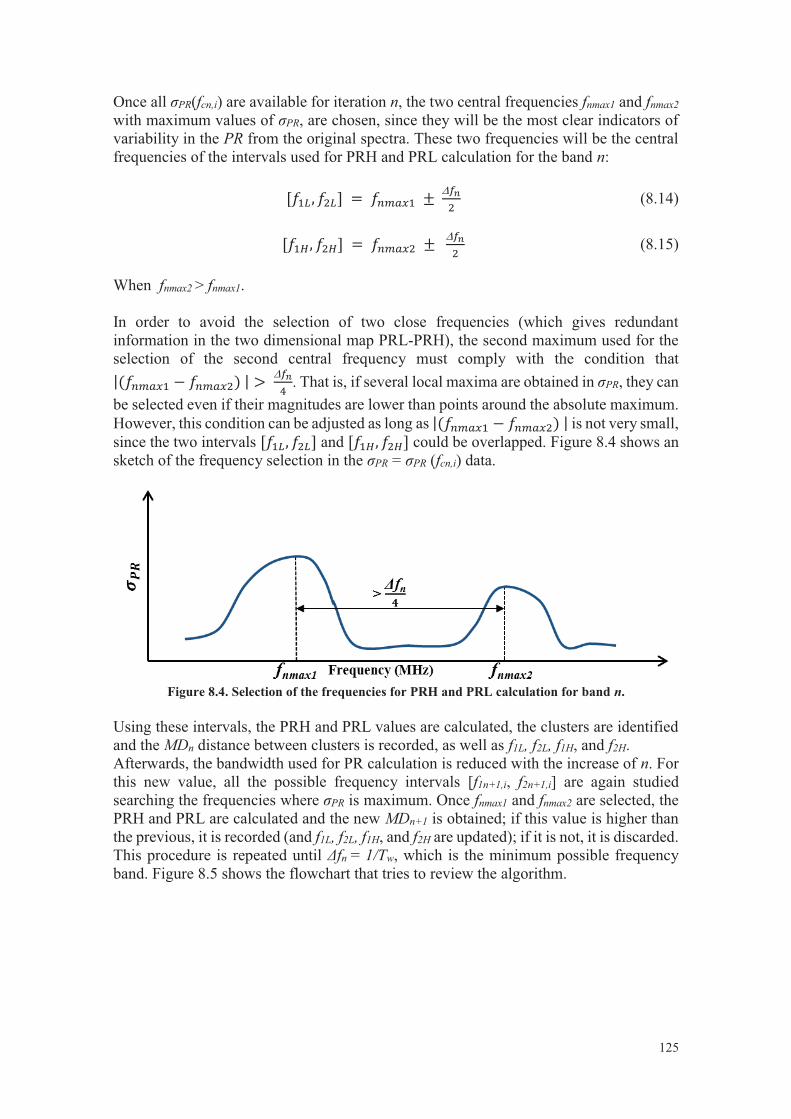
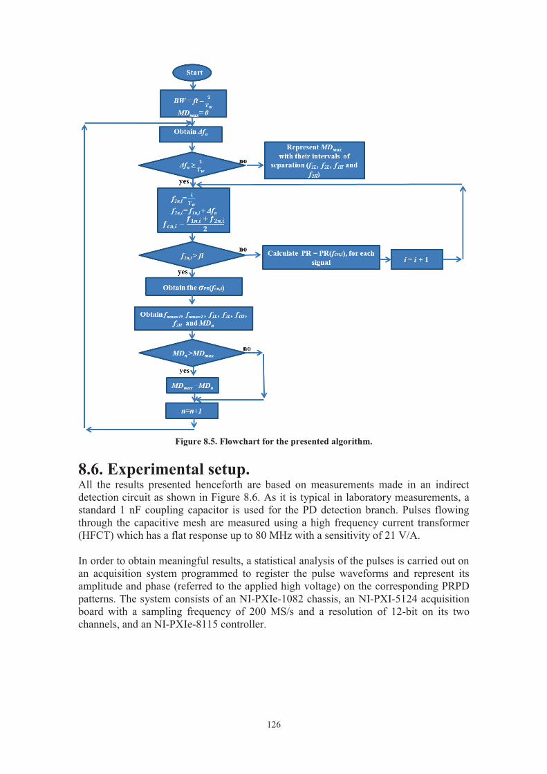
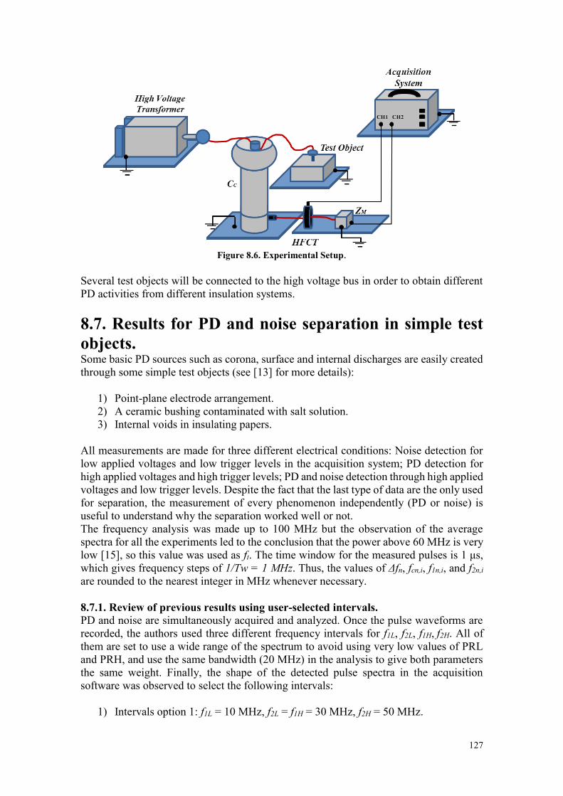
127


Several test objects will be connected to the high voltage bus in order to obtain different PD activities from different insulation systems. 8.7. Results for PD and noise separation in simple test objects. Some basic PD sources such as corona, surface and internal discharges are easily created through some simple test objects (see [13] for more details):

1) Point-plane electrode arrangement. 2) A ceramic bushing contaminated with salt solution. 3) Internal voids in insulating papers.

All measurements are made for three different electrical conditions: Noise detection for low applied voltages and low trigger levels in the acquisition system; PD detection for high applied voltages and high trigger levels; PD and noise detection through high applied voltages and low trigger levels. Despite the fact that the last type of data are the only used for separation, the measurement of every phenomenon independently (PD or noise) is useful to understand why the separation worked well or not. The frequency analysis was made up to 100 MHz but the observation of the average spectra for all the experiments led to the conclusion that the power above 60 MHz is very low [15], so this value was used as ft. The time window for the measured pulses is 1 μs, which gives frequency steps of 1/Tw = 1 MHz. Thus, the values of Δfn, fcn,i, f1n,i, and f2n,i are rounded to the nearest integer in MHz whenever necessary. 8.7.1. Review of previous results using user-selected intervals. PD and noise are simultaneously acquired and analyzed. Once the pulse waveforms are recorded, the authors used three different frequency intervals for f1L, f2L, f1H, f2H. All of them are set to use a wide range of the spectrum to avoid using very low values of PRL and PRH, and use the same bandwidth (20 MHz) in the analysis to give both parameters the same weight. Finally, the shape of the detected pulse spectra in the acquisition software was observed to select the following intervals:

1) Intervals option 1: f1L = 10 MHz, f2L = f1H = 30 MHz, f2H = 50 MHz.

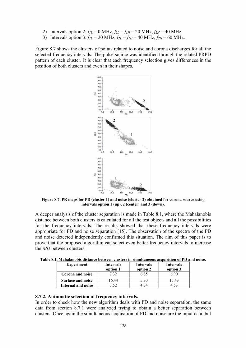
128

2) Intervals option 2: f1L = 0 MHz, f2L = f1H = 20 MHz, f2H = 40 MHz. 3) Intervals option 3: f1L = 20 MHz, f2L = f1H = 40 MHz, f2H = 60 MHz.

Figure 8.7 shows the clusters of points related to noise and corona discharges for all the selected frequency intervals. The pulse source was identified through the related PRPD pattern of each cluster. It is clear that each frequency selection gives differences in the position of both clusters and even in their shapes.

Figure 8.7. PR maps for PD (cluster 1) and noise (cluster 2) obtained for corona source using

intervals option 1 (up), 2 (center) and 3 (down).

A deeper analysis of the cluster separation is made in Table 8.1, where the Mahalanobis distance between both clusters is calculated for all the test objects and all the possibilities for the frequency intervals. The results showed that these frequency intervals were appropriate for PD and noise separation [15]. The observation of the spectra of the PD and noise detected independently confirmed this situation. The aim of this paper is to prove that the proposed algorithm can select even better frequency intervals to increase the MD between clusters.

Table 8.1. Mahalanobis distance between clusters in simultaneous acquisition of PD and noise. Experiment Intervals

option 1 Intervals option 2

Intervals option 3

Corona and noise 7.32 6.85 6.90 Surface and noise 16.44 5.90 15.43 Internal and noise 7.52 4.74 4.53

8.7.2. Automatic selection of frequency intervals. In order to check how the new algorithm deals with PD and noise separation, the same data from section 8.7.1 were analyzed trying to obtain a better separation between clusters. Once again the simultaneous acquisition of PD and noise are the input data, but

1

2

2

1

1

2

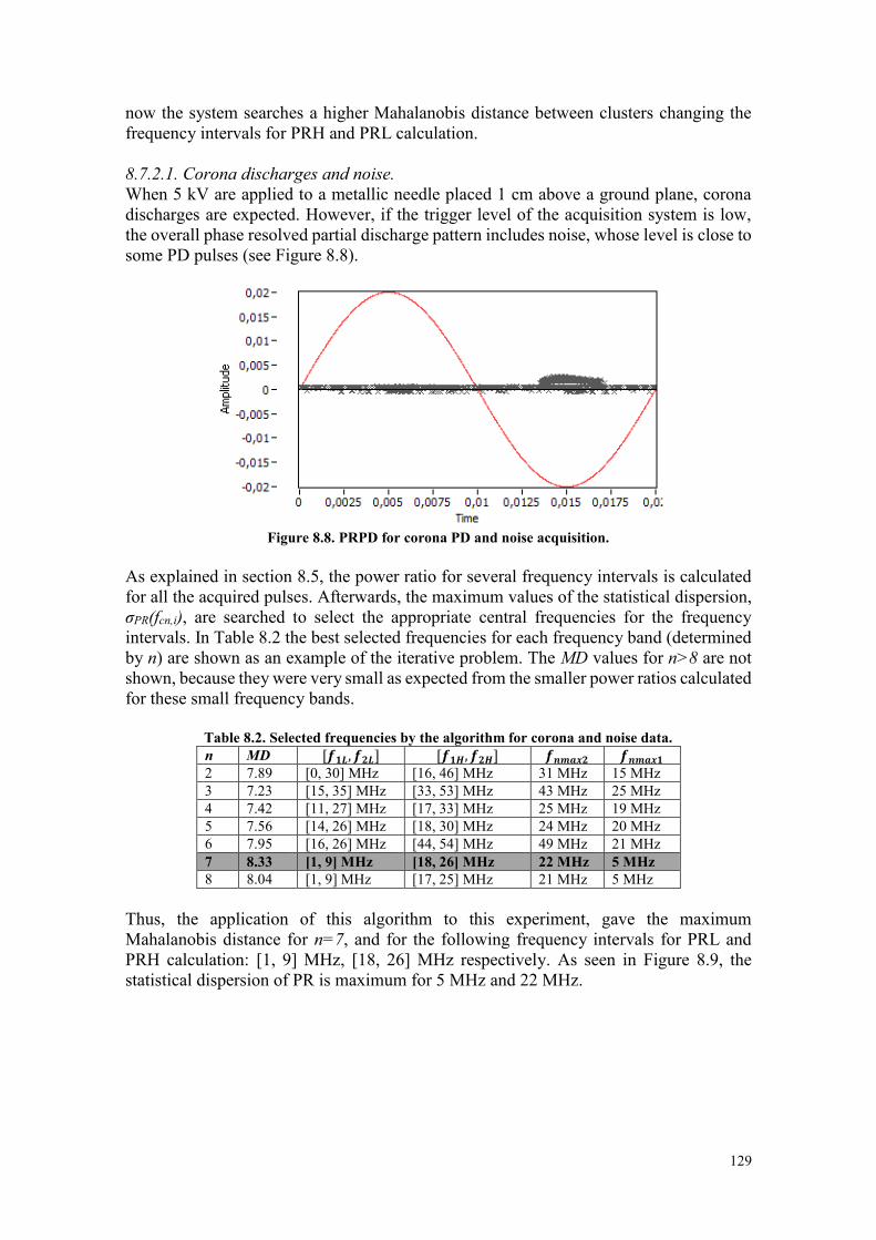
129

now the system searches a higher Mahalanobis distance between clusters changing the frequency intervals for PRH and PRL calculation. 8.7.2.1. Corona discharges and noise. When 5 kV are applied to a metallic needle placed 1 cm above a ground plane, corona discharges are expected. However, if the trigger level of the acquisition system is low, the overall phase resolved partial discharge pattern includes noise, whose level is close to some PD pulses (see Figure 8.8).

Figure 8.8. PRPD for corona PD and noise acquisition.

As explained in section 8.5, the power ratio for several frequency intervals is calculated for all the acquired pulses. Afterwards, the maximum values of the statistical dispersion, σPR(fcn,i), are searched to select the appropriate central frequencies for the frequency intervals. In Table 8.2 the best selected frequencies for each frequency band (determined by n) are shown as an example of the iterative problem. The MD values for n>8 are not shown, because they were very small as expected from the smaller power ratios calculated for these small frequency bands.

Table 8.2. Selected frequencies by the algorithm for corona and noise data. n MD [𝒇𝟏𝑳, 𝒇𝟐𝑳] [𝒇𝟏𝑯, 𝒇𝟐𝑯] 𝒇𝒏𝒎𝒂𝒙𝟐 𝒇𝒏𝒎𝒂𝒙𝟏 2 7.89 [0, 30] MHz [16, 46] MHz 31 MHz 15 MHz 3 7.23 [15, 35] MHz [33, 53] MHz 43 MHz 25 MHz 4 7.42 [11, 27] MHz [17, 33] MHz 25 MHz 19 MHz 5 7.56 [14, 26] MHz [18, 30] MHz 24 MHz 20 MHz 6 7.95 [16, 26] MHz [44, 54] MHz 49 MHz 21 MHz 7 8.33 [1, 9] MHz [18, 26] MHz 22 MHz 5 MHz 8 8.04 [1, 9] MHz [17, 25] MHz 21 MHz 5 MHz

Thus, the application of this algorithm to this experiment, gave the maximum Mahalanobis distance for n=7, and for the following frequency intervals for PRL and PRH calculation: [1, 9] MHz, [18, 26] MHz respectively. As seen in Figure 8.9, the statistical dispersion of PR is maximum for 5 MHz and 22 MHz.

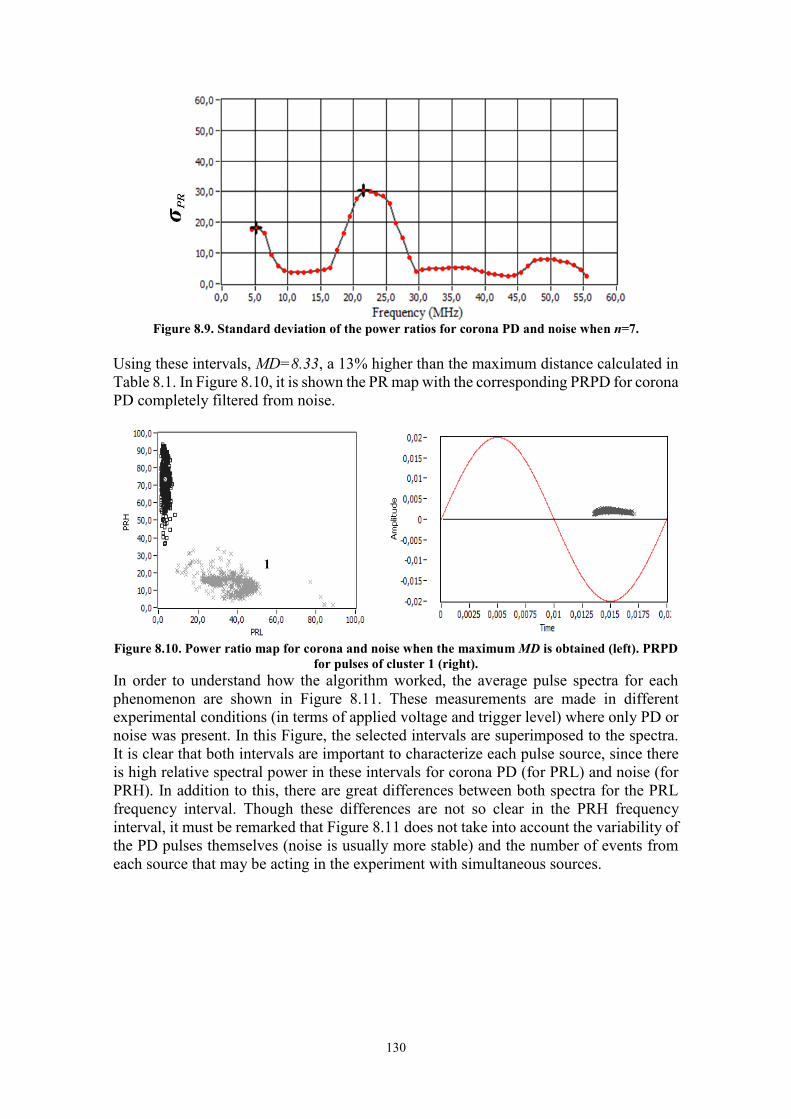
130

Figure 8.9. Standard deviation of the power ratios for corona PD and noise when n=7.

Using these intervals, MD=8.33, a 13% higher than the maximum distance calculated in Table 8.1. In Figure 8.10, it is shown the PR map with the corresponding PRPD for corona PD completely filtered from noise.

Figure 8.10. Power ratio map for corona and noise when the maximum MD is obtained (left). PRPD

for pulses of cluster 1 (right). In order to understand how the algorithm worked, the average pulse spectra for each phenomenon are shown in Figure 8.11. These measurements are made in different experimental conditions (in terms of applied voltage and trigger level) where only PD or noise was present. In this Figure, the selected intervals are superimposed to the spectra. It is clear that both intervals are important to characterize each pulse source, since there is high relative spectral power in these intervals for corona PD (for PRL) and noise (for PRH). In addition to this, there are great differences between both spectra for the PRL frequency interval. Though these differences are not so clear in the PRH frequency interval, it must be remarked that Figure 8.11 does not take into account the variability of the PD pulses themselves (noise is usually more stable) and the number of events from each source that may be acting in the experiment with simultaneous sources.

1

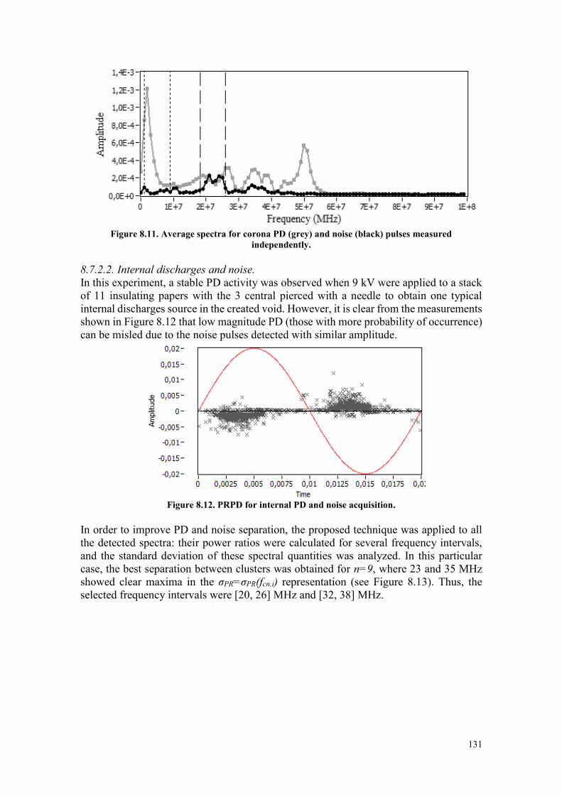
131

Figure 8.11. Average spectra for corona PD (grey) and noise (black) pulses measured

independently. 8.7.2.2. Internal discharges and noise. In this experiment, a stable PD activity was observed when 9 kV were applied to a stack of 11 insulating papers with the 3 central pierced with a needle to obtain one typical internal discharges source in the created void. However, it is clear from the measurements shown in Figure 8.12 that low magnitude PD (those with more probability of occurrence) can be misled due to the noise pulses detected with similar amplitude.

Figure 8.12. PRPD for internal PD and noise acquisition.

In order to improve PD and noise separation, the proposed technique was applied to all the detected spectra: their power ratios were calculated for several frequency intervals, and the standard deviation of these spectral quantities was analyzed. In this particular case, the best separation between clusters was obtained for n=9, where 23 and 35 MHz showed clear maxima in the σPR=σPR(fcn,i) representation (see Figure 8.13). Thus, the selected frequency intervals were [20, 26] MHz and [32, 38] MHz.

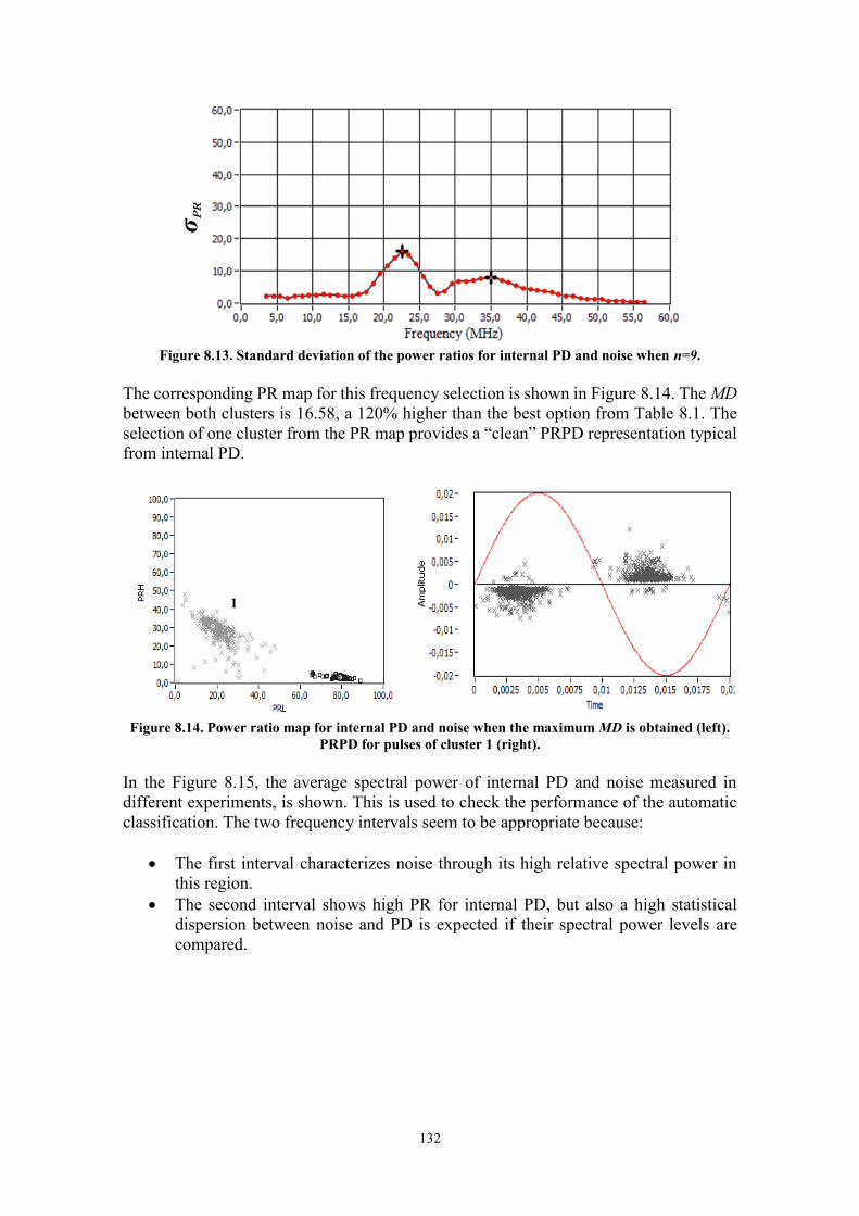
132

Figure 8.13. Standard deviation of the power ratios for internal PD and noise when n=9.

The corresponding PR map for this frequency selection is shown in Figure 8.14. The MD between both clusters is 16.58, a 120% higher than the best option from Table 8.1. The selection of one cluster from the PR map provides a “clean” PRPD representation typical from internal PD.

Figure 8.14. Power ratio map for internal PD and noise when the maximum MD is obtained (left).

PRPD for pulses of cluster 1 (right).

In the Figure 8.15, the average spectral power of internal PD and noise measured in different experiments, is shown. This is used to check the performance of the automatic classification. The two frequency intervals seem to be appropriate because:

The first interval characterizes noise through its high relative spectral power in this region.

The second interval shows high PR for internal PD, but also a high statistical dispersion between noise and PD is expected if their spectral power levels are compared.

1

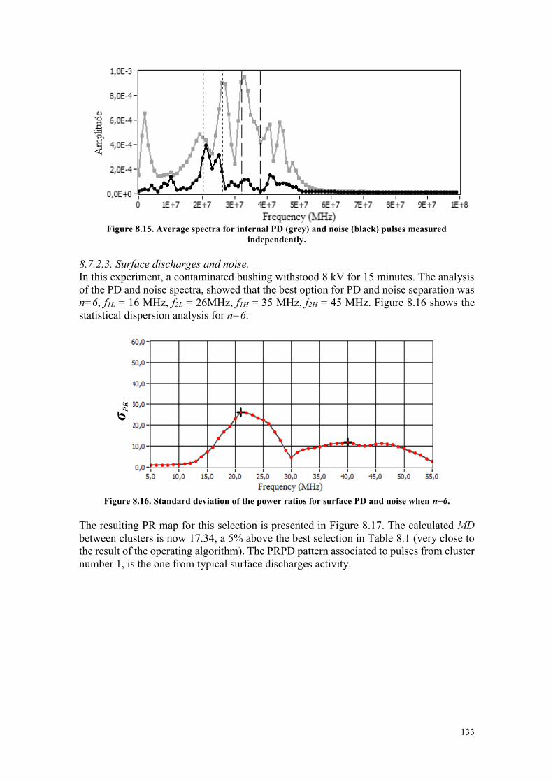
133

Figure 8.15. Average spectra for internal PD (grey) and noise (black) pulses measured

independently.

8.7.2.3. Surface discharges and noise. In this experiment, a contaminated bushing withstood 8 kV for 15 minutes. The analysis of the PD and noise spectra, showed that the best option for PD and noise separation was n=6, f1L = 16 MHz, f2L = 26MHz, f1H = 35 MHz, f2H = 45 MHz. Figure 8.16 shows the statistical dispersion analysis for n=6.

Figure 8.16. Standard deviation of the power ratios for surface PD and noise when n=6.

The resulting PR map for this selection is presented in Figure 8.17. The calculated MD between clusters is now 17.34, a 5% above the best selection in Table 8.1 (very close to the result of the operating algorithm). The PRPD pattern associated to pulses from cluster number 1, is the one from typical surface discharges activity.

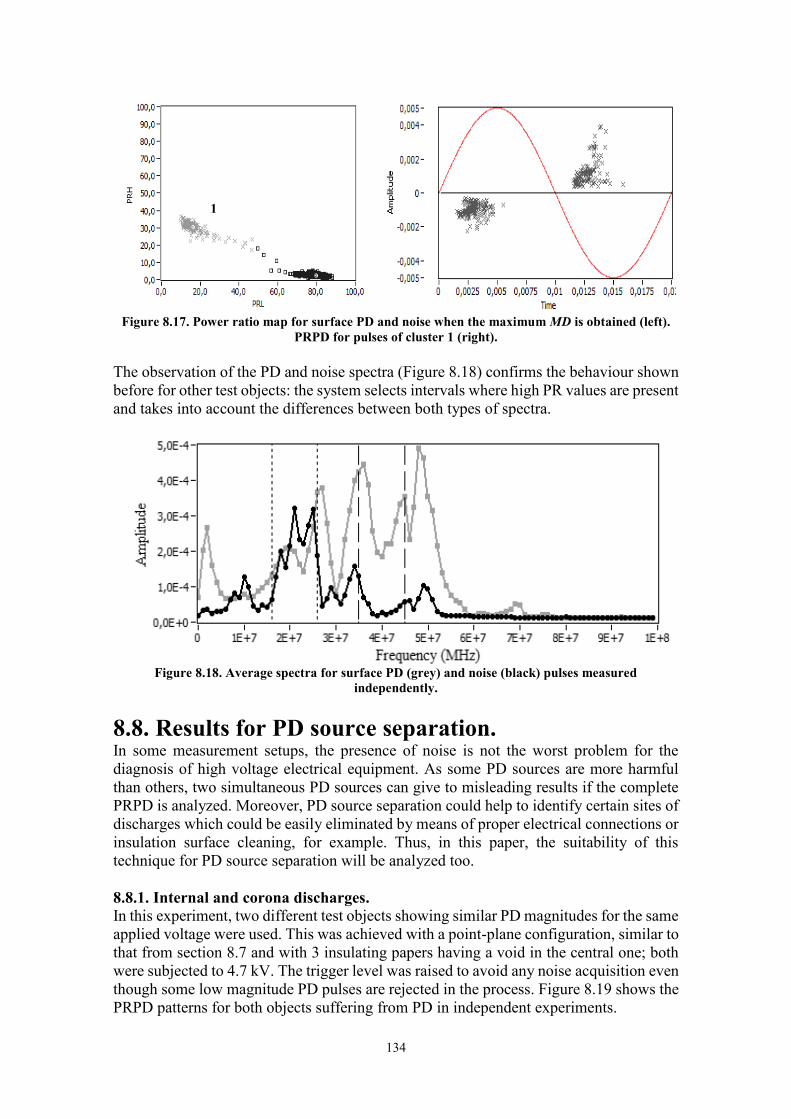
134

Figure 8.17. Power ratio map for surface PD and noise when the maximum MD is obtained (left).

PRPD for pulses of cluster 1 (right).

The observation of the PD and noise spectra (Figure 8.18) confirms the behaviour shown before for other test objects: the system selects intervals where high PR values are present and takes into account the differences between both types of spectra.

Figure 8.18. Average spectra for surface PD (grey) and noise (black) pulses measured

independently.

8.8. Results for PD source separation. In some measurement setups, the presence of noise is not the worst problem for the diagnosis of high voltage electrical equipment. As some PD sources are more harmful than others, two simultaneous PD sources can give to misleading results if the complete PRPD is analyzed. Moreover, PD source separation could help to identify certain sites of discharges which could be easily eliminated by means of proper electrical connections or insulation surface cleaning, for example. Thus, in this paper, the suitability of this technique for PD source separation will be analyzed too. 8.8.1. Internal and corona discharges. In this experiment, two different test objects showing similar PD magnitudes for the same applied voltage were used. This was achieved with a point-plane configuration, similar to that from section 8.7 and with 3 insulating papers having a void in the central one; both were subjected to 4.7 kV. The trigger level was raised to avoid any noise acquisition even though some low magnitude PD pulses are rejected in the process. Figure 8.19 shows the PRPD patterns for both objects suffering from PD in independent experiments.

1

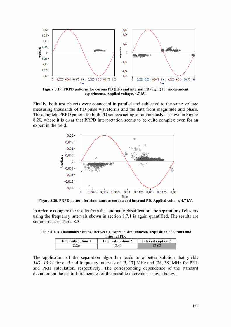
135

Figure 8.19. PRPD patterns for corona PD (left) and internal PD (right) for independent

experiments. Applied voltage, 4.7 kV.

Finally, both test objects were connected in parallel and subjected to the same voltage measuring thousands of PD pulse waveforms and the data from magnitude and phase. The complete PRPD pattern for both PD sources acting simultaneously is shown in Figure 8.20, where it is clear that PRPD interpretation seems to be quite complex even for an expert in the field.

Figure 8.20. PRPD pattern for simultaneous corona and internal PD. Applied voltage, 4.7 kV.

In order to compare the results from the automatic classification, the separation of clusters using the frequency intervals shown in section 8.7.1 is again quantified. The results are summarized in Table 8.3.

Table 8.3. Mahalanobis distance between clusters in simultaneous acquisition of corona and internal PD.

Intervals option 1 Intervals option 2 Intervals option 3 8.86 12.45 12.62

The application of the separation algorithm leads to a better solution that yields MD=13.91 for n=5 and frequency intervals of [5, 17] MHz and [26, 38] MHz for PRL and PRH calculation, respectively. The corresponding dependence of the standard deviation on the central frequencies of the possible intervals is shown below.

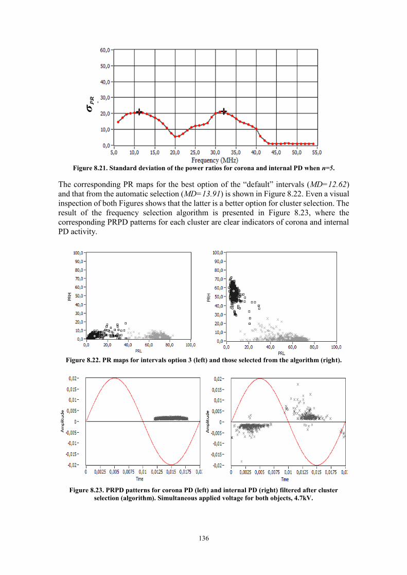
136

Figure 8.21. Standard deviation of the power ratios for corona and internal PD when n=5.

The corresponding PR maps for the best option of the “default” intervals (MD=12.62) and that from the automatic selection (MD=13.91) is shown in Figure 8.22. Even a visual inspection of both Figures shows that the latter is a better option for cluster selection. The result of the frequency selection algorithm is presented in Figure 8.23, where the corresponding PRPD patterns for each cluster are clear indicators of corona and internal PD activity.

Figure 8.22. PR maps for intervals option 3 (left) and those selected from the algorithm (right).

Figure 8.23. PRPD patterns for corona PD (left) and internal PD (right) filtered after cluster

selection (algorithm). Simultaneous applied voltage for both objects, 4.7kV.

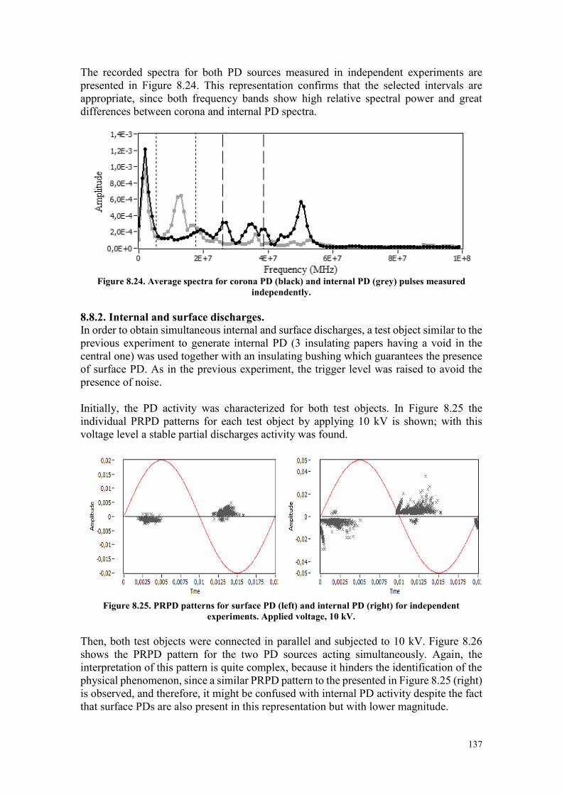
137

The recorded spectra for both PD sources measured in independent experiments are presented in Figure 8.24. This representation confirms that the selected intervals are appropriate, since both frequency bands show high relative spectral power and great differences between corona and internal PD spectra.

Figure 8.24. Average spectra for corona PD (black) and internal PD (grey) pulses measured

independently.

8.8.2. Internal and surface discharges. In order to obtain simultaneous internal and surface discharges, a test object similar to the previous experiment to generate internal PD (3 insulating papers having a void in the central one) was used together with an insulating bushing which guarantees the presence of surface PD. As in the previous experiment, the trigger level was raised to avoid the presence of noise. Initially, the PD activity was characterized for both test objects. In Figure 8.25 the individual PRPD patterns for each test object by applying 10 kV is shown; with this voltage level a stable partial discharges activity was found.

Figure 8.25. PRPD patterns for surface PD (left) and internal PD (right) for independent

experiments. Applied voltage, 10 kV.

Then, both test objects were connected in parallel and subjected to 10 kV. Figure 8.26 shows the PRPD pattern for the two PD sources acting simultaneously. Again, the interpretation of this pattern is quite complex, because it hinders the identification of the physical phenomenon, since a similar PRPD pattern to the presented in Figure 8.25 (right) is observed, and therefore, it might be confused with internal PD activity despite the fact that surface PDs are also present in this representation but with lower magnitude.

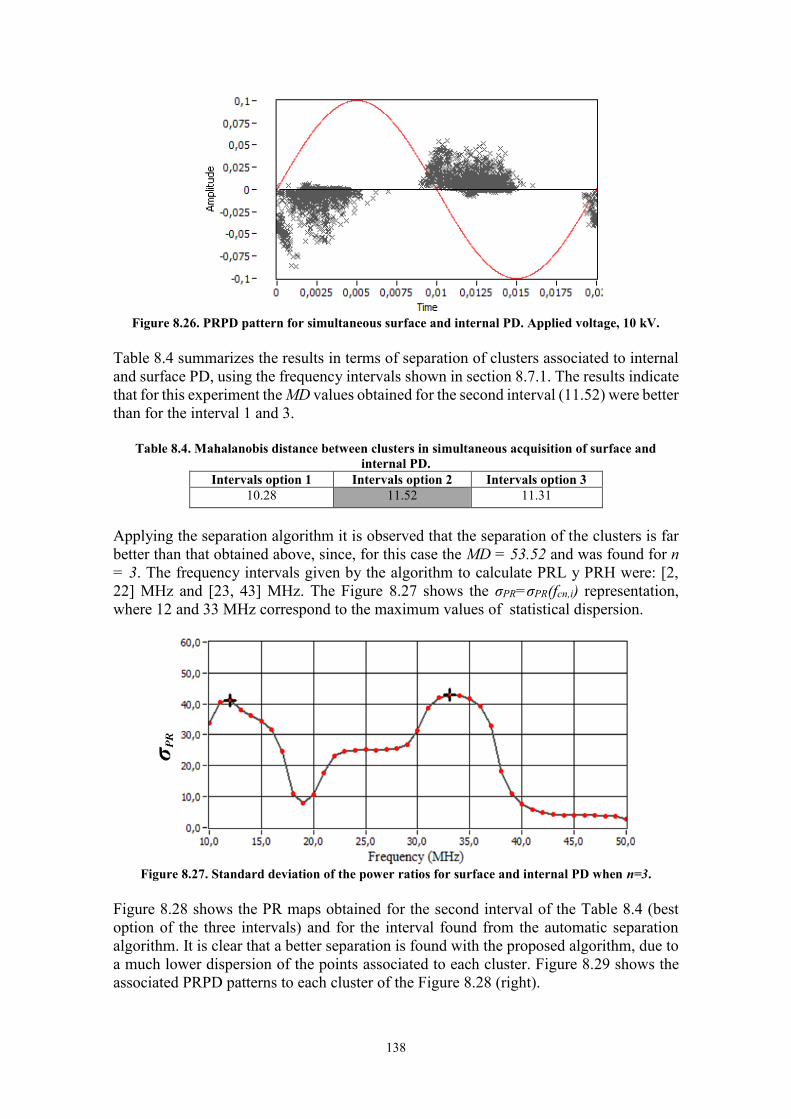
138

Figure 8.26. PRPD pattern for simultaneous surface and internal PD. Applied voltage, 10 kV.

Table 8.4 summarizes the results in terms of separation of clusters associated to internal and surface PD, using the frequency intervals shown in section 8.7.1. The results indicate that for this experiment the MD values obtained for the second interval (11.52) were better than for the interval 1 and 3.

Table 8.4. Mahalanobis distance between clusters in simultaneous acquisition of surface and internal PD.

Intervals option 1 Intervals option 2 Intervals option 3 10.28 11.52 11.31

Applying the separation algorithm it is observed that the separation of the clusters is far better than that obtained above, since, for this case the MD = 53.52 and was found for n = 3. The frequency intervals given by the algorithm to calculate PRL y PRH were: [2, 22] MHz and [23, 43] MHz. The Figure 8.27 shows the σPR=σPR(fcn,i) representation, where 12 and 33 MHz correspond to the maximum values of statistical dispersion.

Figure 8.27. Standard deviation of the power ratios for surface and internal PD when n=3.

Figure 8.28 shows the PR maps obtained for the second interval of the Table 8.4 (best option of the three intervals) and for the interval found from the automatic separation algorithm. It is clear that a better separation is found with the proposed algorithm, due to a much lower dispersion of the points associated to each cluster. Figure 8.29 shows the associated PRPD patterns to each cluster of the Figure 8.28 (right).

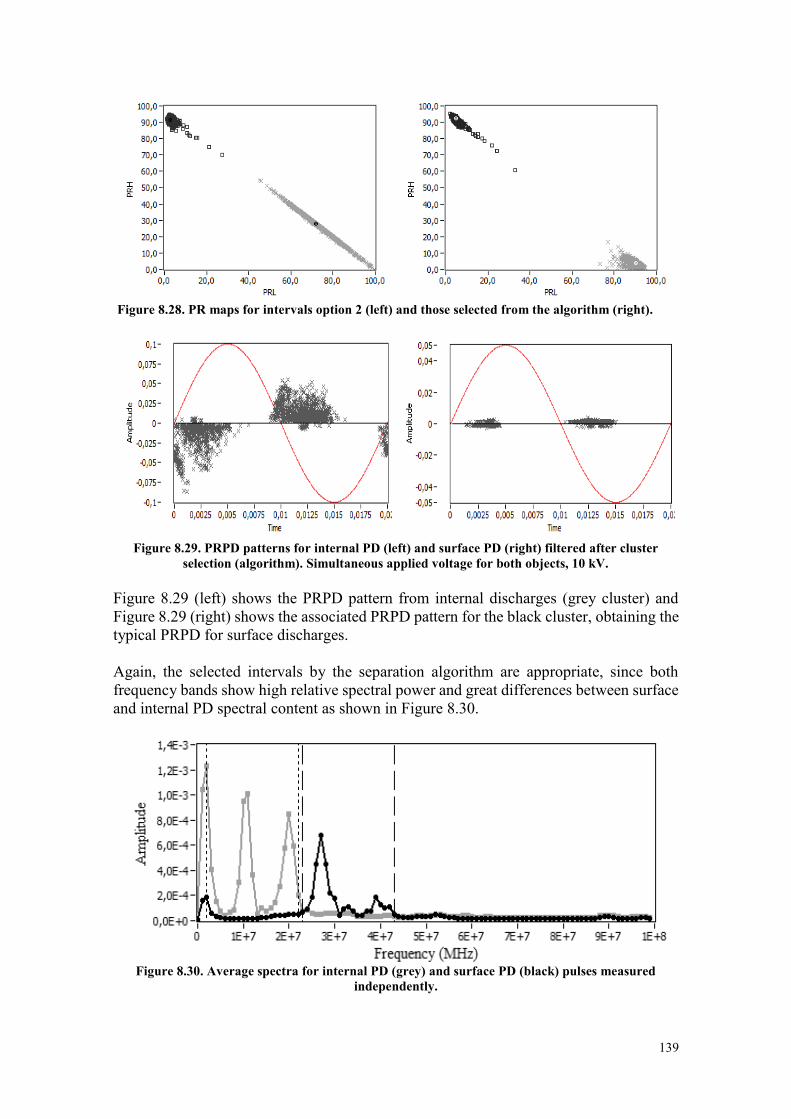
139

Figure 8.28. PR maps for intervals option 2 (left) and those selected from the algorithm (right).

Figure 8.29. PRPD patterns for internal PD (left) and surface PD (right) filtered after cluster

selection (algorithm). Simultaneous applied voltage for both objects, 10 kV.

Figure 8.29 (left) shows the PRPD pattern from internal discharges (grey cluster) and Figure 8.29 (right) shows the associated PRPD pattern for the black cluster, obtaining the typical PRPD for surface discharges. Again, the selected intervals by the separation algorithm are appropriate, since both frequency bands show high relative spectral power and great differences between surface and internal PD spectral content as shown in Figure 8.30.

Figure 8.30. Average spectra for internal PD (grey) and surface PD (black) pulses measured

independently.

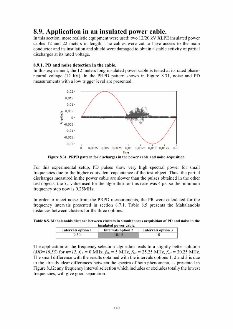
140

8.9. Application in an insulated power cable. In this section, more realistic equipment were used: two 12/20 kV XLPE insulated power cables 12 and 22 meters in length. The cables were cut to have access to the main conductor and its insulation and shield were damaged to obtain a stable activity of partial discharges at its rated voltage. 8.9.1. PD and noise detection in the cable. In this experiment, the 12 meters long insulated power cable is tested at its rated phase-neutral voltage (12 kV). In the PRPD pattern shown in Figure 8.31, noise and PD measurements with a low trigger level are presented.

Figure 8.31. PRPD pattern for discharges in the power cable and noise acquisition.

For this experimental setup, PD pulses show very high spectral power for small frequencies due to the higher equivalent capacitance of the test object. Thus, the partial discharges measured in the power cable are slower than the pulses obtained in the other test objects; the Tw value used for the algorithm for this case was 4 µs, so the minimum frequency step now is 0.25MHz. In order to reject noise from the PRPD measurements, the PR were calculated for the frequency intervals presented in section 8.7.1. Table 8.5 presents the Mahalanobis distances between clusters for the three options. Table 8.5. Mahalanobis distance between clusters in simultaneous acquisition of PD and noise in the

insulated power cable. Intervals option 1 Intervals option 2 Intervals option 3

9.50 10.15 10

The application of the frequency selection algorithm leads to a slightly better solution (MD=10.55) for n=12, f1L = 0 MHz, f2L = 5 MHz, f1H = 25.25 MHz, f2H = 30.25 MHz. The small difference with the results obtained with the intervals options 1, 2 and 3 is due to the already clear differences between the spectra of both phenomena, as presented in Figure 8.32: any frequency interval selection which includes or excludes totally the lowest frequencies, will give good separation.

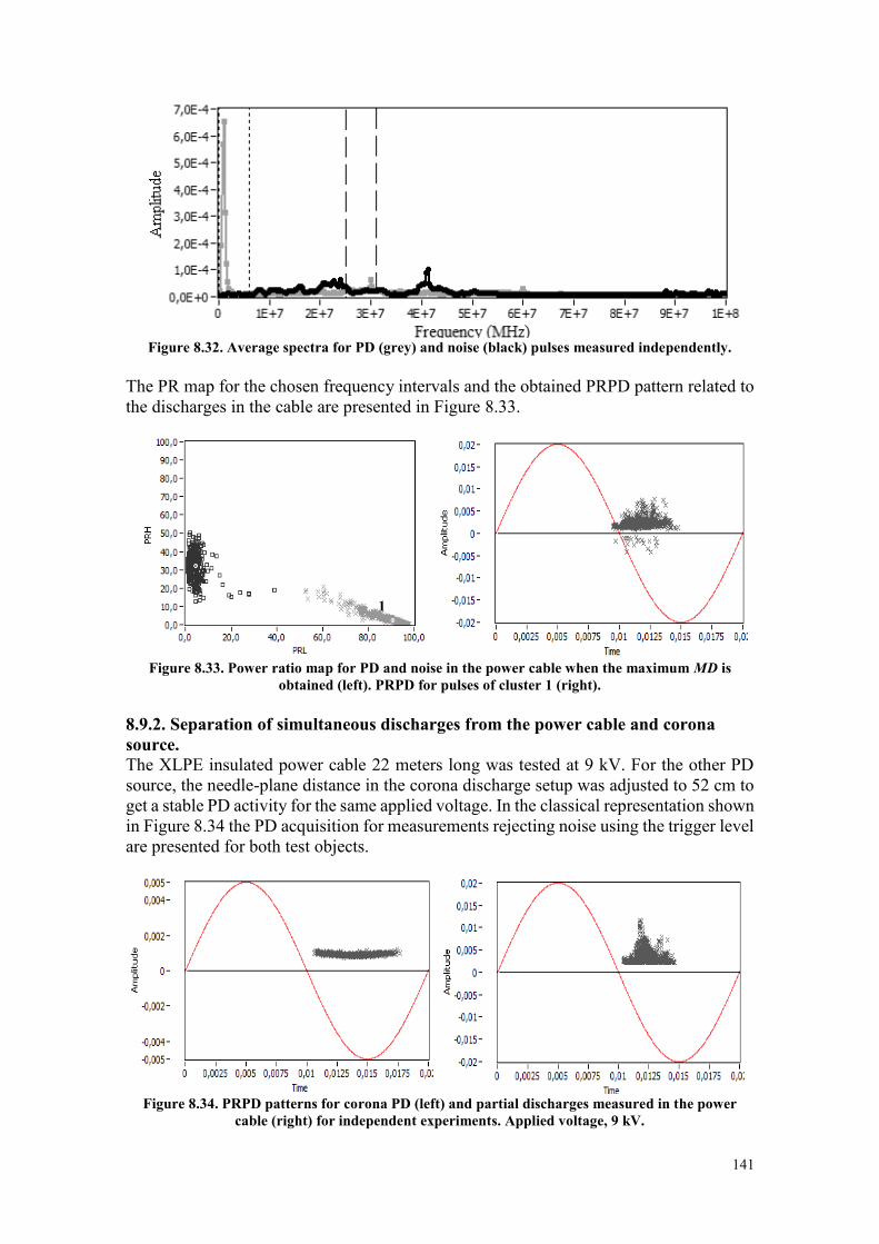
141

Figure 8.32. Average spectra for PD (grey) and noise (black) pulses measured independently.

The PR map for the chosen frequency intervals and the obtained PRPD pattern related to the discharges in the cable are presented in Figure 8.33.

Figure 8.33. Power ratio map for PD and noise in the power cable when the maximum MD is

obtained (left). PRPD for pulses of cluster 1 (right).

8.9.2. Separation of simultaneous discharges from the power cable and corona source. The XLPE insulated power cable 22 meters long was tested at 9 kV. For the other PD source, the needle-plane distance in the corona discharge setup was adjusted to 52 cm to get a stable PD activity for the same applied voltage. In the classical representation shown in Figure 8.34 the PD acquisition for measurements rejecting noise using the trigger level are presented for both test objects.

Figure 8.34. PRPD patterns for corona PD (left) and partial discharges measured in the power

cable (right) for independent experiments. Applied voltage, 9 kV.

1

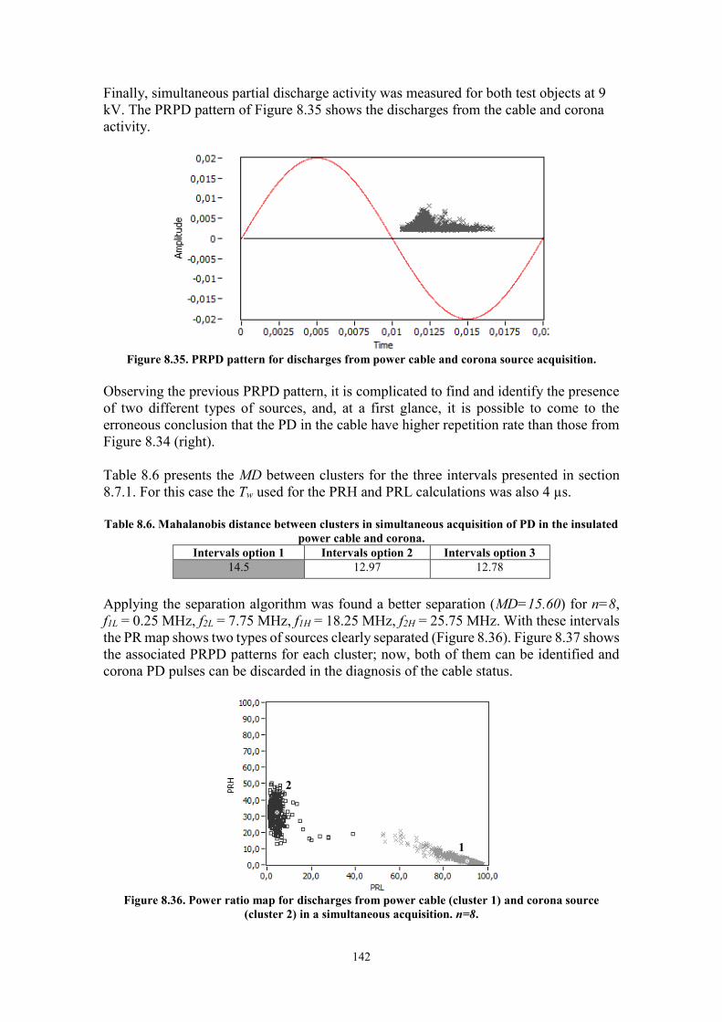
142

Finally, simultaneous partial discharge activity was measured for both test objects at 9 kV. The PRPD pattern of Figure 8.35 shows the discharges from the cable and corona activity.

Figure 8.35. PRPD pattern for discharges from power cable and corona source acquisition.

Observing the previous PRPD pattern, it is complicated to find and identify the presence of two different types of sources, and, at a first glance, it is possible to come to the erroneous conclusion that the PD in the cable have higher repetition rate than those from Figure 8.34 (right). Table 8.6 presents the MD between clusters for the three intervals presented in section 8.7.1. For this case the Tw used for the PRH and PRL calculations was also 4 µs. Table 8.6. Mahalanobis distance between clusters in simultaneous acquisition of PD in the insulated

power cable and corona. Intervals option 1 Intervals option 2 Intervals option 3

14.5 12.97 12.78

Applying the separation algorithm was found a better separation (MD=15.60) for n=8, f1L = 0.25 MHz, f2L = 7.75 MHz, f1H = 18.25 MHz, f2H = 25.75 MHz. With these intervals the PR map shows two types of sources clearly separated (Figure 8.36). Figure 8.37 shows the associated PRPD patterns for each cluster; now, both of them can be identified and corona PD pulses can be discarded in the diagnosis of the cable status.

Figure 8.36. Power ratio map for discharges from power cable (cluster 1) and corona source

(cluster 2) in a simultaneous acquisition. n=8.

1

2

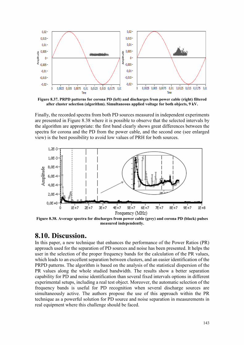
143

Figure 8.37. PRPD patterns for corona PD (left) and discharges from power cable (right) filtered

after cluster selection (algorithm). Simultaneous applied voltage for both objects, 9 kV.

Finally, the recorded spectra from both PD sources measured in independent experiments are presented in Figure 8.38 where it is possible to observe that the selected intervals by the algorithm are appropriate: the first band clearly shows great differences between the spectra for corona and the PD from the power cable, and the second one (see enlarged view) is the best possibility to avoid low values of PRH for both sources.

Figure 8.38. Average spectra for discharges from power cable (grey) and corona PD (black) pulses

measured independently.

8.10. Discussion. In this paper, a new technique that enhances the performance of the Power Ratios (PR) approach used for the separation of PD sources and noise has been presented. It helps the user in the selection of the proper frequency bands for the calculation of the PR values, which leads to an excellent separation between clusters, and an easier identification of the PRPD patterns. The algorithm is based on the analysis of the statistical dispersion of the PR values along the whole studied bandwidth. The results show a better separation capability for PD and noise identification than several fixed intervals options in different experimental setups, including a real test object. Moreover, the automatic selection of the frequency bands is useful for PD recognition when several discharge sources are simultaneously active. The authors propose the use of this approach within the PR technique as a powerful solution for PD source and noise separation in measurements in real equipment where this challenge should be faced.

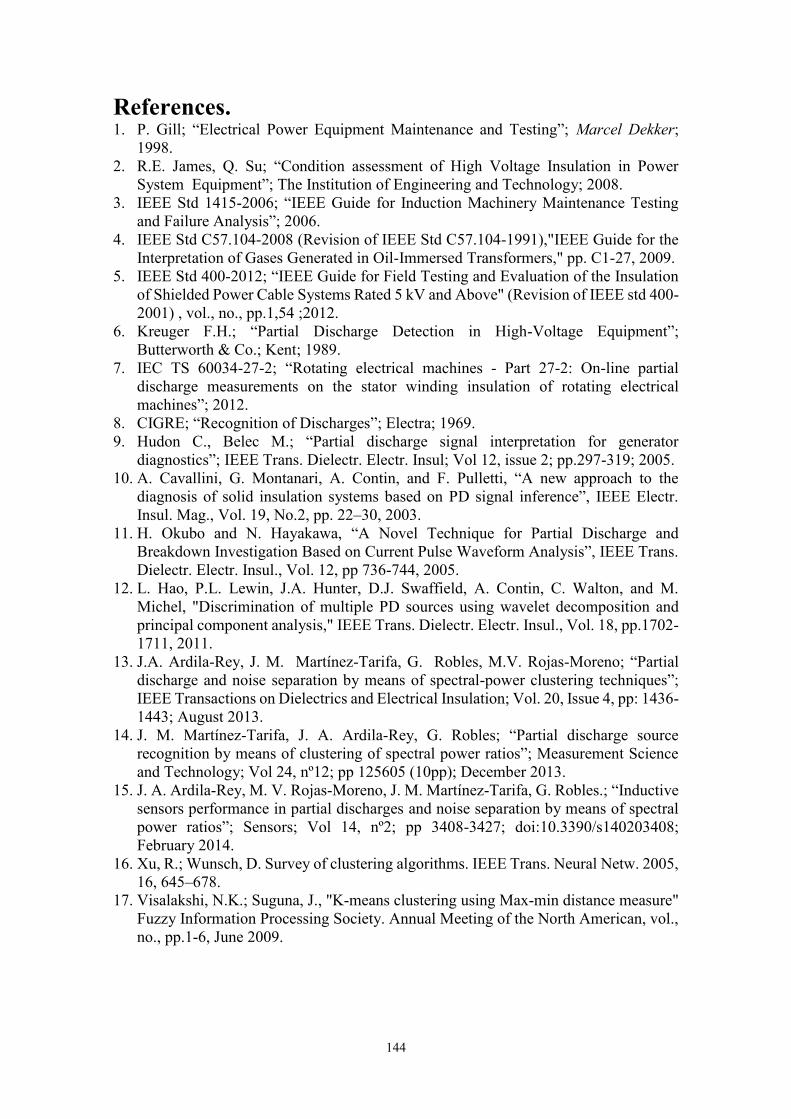
144

References. 1. P. Gill; “Electrical Power Equipment Maintenance and Testing”; Marcel Dekker;

1998. 2. R.E. James, Q. Su; “Condition assessment of High Voltage Insulation in Power

System Equipment”; The Institution of Engineering and Technology; 2008. 3. IEEE Std 1415-2006; “IEEE Guide for Induction Machinery Maintenance Testing

and Failure Analysis”; 2006. 4. IEEE Std C57.104-2008 (Revision of IEEE Std C57.104-1991),"IEEE Guide for the

Interpretation of Gases Generated in Oil-Immersed Transformers," pp. C1-27, 2009. 5. IEEE Std 400-2012; “IEEE Guide for Field Testing and Evaluation of the Insulation

of Shielded Power Cable Systems Rated 5 kV and Above" (Revision of IEEE std 400-2001) , vol., no., pp.1,54 ;2012.

6. Kreuger F.H.; “Partial Discharge Detection in High-Voltage Equipment”; Butterworth & Co.; Kent; 1989.

7. IEC TS 60034-27-2; “Rotating electrical machines - Part 27-2: On-line partial discharge measurements on the stator winding insulation of rotating electrical machines”; 2012.

8. CIGRE; “Recognition of Discharges”; Electra; 1969. 9. Hudon C., Belec M.; “Partial discharge signal interpretation for generator

diagnostics”; IEEE Trans. Dielectr. Electr. Insul; Vol 12, issue 2; pp.297-319; 2005. 10. A. Cavallini, G. Montanari, A. Contin, and F. Pulletti, “A new approach to the

diagnosis of solid insulation systems based on PD signal inference”, IEEE Electr. Insul. Mag., Vol. 19, No.2, pp. 22–30, 2003.

11. H. Okubo and N. Hayakawa, “A Novel Technique for Partial Discharge and Breakdown Investigation Based on Current Pulse Waveform Analysis”, IEEE Trans. Dielectr. Electr. Insul., Vol. 12, pp 736-744, 2005.

12. L. Hao, P.L. Lewin, J.A. Hunter, D.J. Swaffield, A. Contin, C. Walton, and M. Michel, "Discrimination of multiple PD sources using wavelet decomposition and principal component analysis," IEEE Trans. Dielectr. Electr. Insul., Vol. 18, pp.1702-1711, 2011.

13. J.A. Ardila-Rey, J. M. Martínez-Tarifa, G. Robles, M.V. Rojas-Moreno; “Partial discharge and noise separation by means of spectral-power clustering techniques”; IEEE Transactions on Dielectrics and Electrical Insulation; Vol. 20, Issue 4, pp: 1436-1443; August 2013.

14. J. M. Martínez-Tarifa, J. A. Ardila-Rey, G. Robles; “Partial discharge source recognition by means of clustering of spectral power ratios”; Measurement Science and Technology; Vol 24, nº12; pp 125605 (10pp); December 2013.

15. J. A. Ardila-Rey, M. V. Rojas-Moreno, J. M. Martínez-Tarifa, G. Robles.; “Inductive sensors performance in partial discharges and noise separation by means of spectral power ratios”; Sensors; Vol 14, nº2; pp 3408-3427; doi:10.3390/s140203408; February 2014.

16. Xu, R.; Wunsch, D. Survey of clustering algorithms. IEEE Trans. Neural Netw. 2005, 16, 645–678.

17. Visalakshi, N.K.; Suguna, J., "K-means clustering using Max-min distance measure" Fuzzy Information Processing Society. Annual Meeting of the North American, vol., no., pp.1-6, June 2009.

145

Capítulo 9 Conclusiones, aportaciones y trabajos

futuros

Contenidos 9.1. Conclusiones .......................................................................................................... 145 9.2. Aportaciones .......................................................................................................... 146 9.3. Publicaciones ......................................................................................................... 147 9.3.1. Resultados directos. .......................................................................................... 147 9.3.2. Resultados indirectos.. ...................................................................................... 148

9.4. Trabajos futuros ..................................................................................................... 149

9.1. Conclusiones. Desde hace varias décadas, la medida de PDs se ha catalogado como una herramienta útil en el diagnóstico de equipos eléctricos de alta tensión, ya que su actividad está directamente relacionada con diferentes mecanismos de envejecimiento. Tradicionalmente se han utilizado patrones de descarga parcial con resolución en fase (PRPD) para identificar fuentes de PDs y ruido eléctrico. Esta técnica clásica ya normalizada, permite la separación de PDs y ruido mediante la comparación de los valores de magnitud y fase de los pulsos de PDs. Sin embargo, estos patrones solo permiten la identificación de fuentes de PDs cuando están relacionadas con un proceso de degradación claro y cuando el nivel de ruido es bajo en comparación con las amplitudes de las descargas. Sin embargo, en un sistema de aislamiento real es habitual encontrar simultáneamente diversas fuentes de PDs y altos niveles de ruido, especialmente si las mediciones se realizan con el equipo en servicio. Por tal razón, es indispensable la aplicación de técnicas avanzadas de procesamiento de señales con el fin de separar adecuadamente cada una de las fuentes asociadas a PDs y ruido, permitiendo así realizar un diagnóstico más preciso de lo que está ocurriendo en el equipo bajo análisis. En este trabajo se presenta una nueva técnica de separación de fuentes de descargas parciales y ruido, basada en el análisis de las relaciones de potencia espectral PRL (“Power Ratio for Low frequencies”) y PRH (“Power Ratio for High frequencies”). Esta nueva técnica ha demostrado ser capaz de caracterizar con éxito pulsos de PDs y/o ruido de diferente origen, lo que la convierte en una herramienta muy útil a la hora de filtrar señales no deseadas en el diagnóstico de equipos eléctricos. Esta capacidad de caracterización se estudió en el Capítulo 5 de este documento, en donde a través de una serie de experimentos realizados sobre varios objetos de ensayo se demostró que el sistema implementado permite separar en distintas zonas de un mapa de clasificación las fuentes asociadas a PDs (corona, superficiales e internas) y ruido eléctrico. Hay que señalar que una de las grandes ventajas de esta técnica, tal y como se describe en el Capítulo 6, es que permite modificar los intervalos de frecuencia para el cálculo de PRH-PRL dependiendo del espectro observado para cada señal durante la adquisición; esta característica es muy importante, ya que una configuración experimental o entorno

146

industrial diferente puede generar cambios en la ubicación, forma y dispersión de las nubes de puntos representadas, lo que puede complicar la separación mediante otras técnicas con menor flexibilidad en los parámetros empleados. El análisis posterior de los patrones PRPD de las fuentes filtradas ha permitido identificar diferentes tipos de descargas parciales y/o ruido eléctrico. Por otra parte, la respuesta en frecuencia del sensor (que varía de acuerdo a su principio de funcionamiento) pueden llegar también a modificar la caracterización realizada en el mapa de clasificación, lo que se describe en el Capítulo 7 donde se estudió la capacidad de separación de esta técnica para dos sensores inductivos diferentes (transformador de alta frecuencia y lazo inductivo) teniendo en cuenta no solo la distancia o separación entre las nubes de puntos (cluster) sino también la calidad de las mismas, es decir, la dispersión de los puntos asociados a cada cluster. Los resultados obtenidos demuestran que ambos sensores permiten separar adecuadamente diversas fuentes de PDs del ruido eléctrico. El análisis detallado de las agrupaciones de puntos obtenidos para tres selecciones diferentes de intervalos de frecuencia demuestran que el ILS (“Inductive Loop Sensor”, cuyo comportamiento es derivativo hasta 35 MHz), da lugar a clusters que tenían menor dispersión en los ejes PRL y PRH que los obtenidos con el HFCT (“High Frequency Current Transformer”), lo cual permitió obtener para el lazo inductivo una mejor separación entre las nubes de puntos asociadas a cada fuente. Este resultado es de gran relevancia, pues uno de los puntos débiles del sensor ILS es su menor sensibilidad, lo que puede compensarse con su integración en un sistema de separación como éste, que permita detectar descargas parciales aunque tengan magnitudes similares a las del ruido. Adicionalmente, en el Capítulo 8 se presenta el desarrollo de un algoritmo que permite obtener de forma automática unos intervalos de frecuencia adecuados para la separación de las fuentes de descargas y ruido activas. Para ello, se analiza la dispersión estadística de la potencia espectral relativa de las señales bajo análisis. Los resultados obtenidos demuestran que los intervalos de frecuencia seleccionados permiten obtener una muy buena separación entre las nubes de puntos, para múltiples experimentos sobre objetos de ensayos simples e incluso sobre cables aislados de media tensión, tanto para separar ruido de descargas parciales, como para separar diferentes tipos de descargas parciales entre sí. Finalmente, hay que señalar que esta técnica de separación ha sido integrada con éxito en un sistema de adquisición de descargas parciales denominado “PD_LINEALT” y en un sistema de procesamiento off-line llamado “LINEALT_PROCESSING”, los cuales se describen en el Capítulo 4 de esta Tesis. Estos sistemas permiten realizar un procesamiento estadístico riguroso (en términos de magnitud, fase y tasa de repetición) de los patrones resueltos por fase de las fuentes de descargas parciales ya filtradas, lo que ayuda a abordar un diagnóstico adecuado del sistema de aislamiento. Actualmente, ambos sistemas constituyen un importante activo instrumental del Laboratorio de Investigación y Ensayos en Alta Tensión (LINEALT) de la Universidad Carlos III de Madrid. 9.2. Aportaciones. La principal aportación de esta Tesis es la aplicación de una nueva técnica de separación y clasificación de fuentes de PDs y ruido basado en el análisis de la potencia espectral de los pulsos detectados para dos bandas de frecuencia. Con esta técnica se ha logrado caracterizar en un mapa bidimensional las diferentes fuentes que pueden estar presentes durante la adquisición, a través de nubes de puntos (clusters) que se ubican en diferentes partes del mapa de acuerdo a su naturaleza. El sistema ha demostrado ser eficaz tanto en

147

la separación de descargas parciales de ruido eléctrico, como en la caracterización de fuentes simultáneas de descargas parciales. Igualmente, se ha mostrado la compatibilidad del sistema con diversos tipos de sensores inductivos de diferente respuesta en frecuencia. Otra aportación importante, ha sido la implementación de un algoritmo que permite seleccionar de forma automática las bandas de frecuencia de mayor interés con el fin de obtener una mejor separación de los clusters en el mapa de clasificación. Este resultado tiene gran importancia, pues permite ser un apoyo importante para el operador del sistema que pueda no ser un experto en tratamiento de señales o vea demasiada similitud entre los espectros de pulsos detectados. Por último, se ha diseñado e implementado un sistema de adquisición y pre-procesamiento on-line y otro de procesamiento off-line de descargas parciales en los que se ha integrado la técnica de separación propuesta, con el fin de filtrar los clusters asociados a descargas parciales y ruido eléctrico. Una vez seleccionada la fuente de descargas parciales, el software permite realizar estimaciones estadísticas fiables sobre magnitudes, fases y tasa de repetición de las PDs detectadas. 9.3. Publicaciones. Fruto de este trabajo de investigación, se han obtenido resultados que han sido divulgados en diversos foros. Algunas de las publicaciones desarrolladas están directamente relacionadas con esta Tesis doctoral, mientras que otras, aunque están también focalizadas en la detección, monitorización y análisis de descargas parciales mediante otras técnicas de medida, tienen una relación con este trabajo más indirecta. 9.3.1. Resultados directos. Revistas indexadas en el Journal Citation Report:

Ardila-Rey J, Martin z-Tarifa J, Robles G, Rojas-Moreno M; “Partial discharge and noise separation by means of spectral-power clustering techniques”; Dielectrics and Electrical Insulation, IEEE Transactions, vol.20, no.4, pp.1436-1443, August 2013.

Martínez-Tarifa J. M, Ardila-Rey J. A, Robles G; “Partial discharge source recognition by means of clustering of spectral power ratios”; Measurement Science and Technology, Vol 24, nº12; pp 125605 (10pp), December 2013.

Ardila-Rey J. A, Rojas-Moreno M. V, Martínez-Tarifa J. M, Robles G; “Inductive Sensor Performance in Partial Discharges and Noise Separation by Means of Spectral Power Ratios”; Sensors 14, no 2, pp 3408-3427, 2014.

Martínez-Tarifa J. M, Ardila-Rey J. A, Robles G; “Automatic selection of frequency bands for the power ratios separation technique in partial discharge measurements”; (Enviado a Dielectrics and Electrical Insulation, IEEE Transactions, en Junio de 2014).

148

Congresos Internacionales: Ardila-Rey J. A, Martinez-Tarifa J. M, Robles G, Rojas-Moreno M, Albarracin

R; “A Partial Discharges acquisition and statistical analysis software”; Instrumentation and Measurement Technology Conference (I2MTC), 2012 IEEE International, vol, pp.1670-1675, 13-16 May 2012.

Patente: Ardila-Rey J. A, Martinez-Tarifa J. M, Robles G; Oficina Española de Patentes y

Marcas; “Método y dispositivo para la diferenciación de descargas parciales y ruido eléctrico”; No: P201330413, 22 Marzo 2013 (Solicitud de PCT en Marzo de 2014).

Revistas y conferencias de ámbito nacional: Ardila-Rey J. A; Conferencia invitada para las Jornadas de Ingeniería organizadas

por “Laureate International Universities” y la Universidad Europea de Madrid. “Análisis y detección de descargas parciales”; 2012; España.

Ardila-Rey J. A, Martínez-Tarifa J. M, Robles G; “Desarrollo e implementación de un sistema de adquisición de descargas parciales”; Revista Tecnológica sobre diseño gráfico de sistemas, LabVIEW NI Days; Febrero 2013; Barcelona.

9.3.2. Resultados indirectos. Revistas indexadas en el Journal Citation Report:

Rojas M, Robles G, Albarracín R, Ardila-Rey J. A, Martínez-Tarifa, J.M; “Study of a Rogowski coil as a versatile sensor for measuring high frequency current pulses”; Electronics and Electrical Engineering (Enviado el 13 de Marzo de 2014).

Parrado-Hernandez E, Robles G, Ardila-Rey J.A, Martínez-Tarifa J.M; “Partial

discharge discrimination with support vector machines”; Electric Power Systems Research. (En revisión).

Congresos internacionales:

Robles G, Martinez-Tarifa J. M, Rojas-Moreno M. V, Albarracin R, Ardila-Rey J; “Antenna selection and frequency response study for UHF detection of partial discharges”; Instrumentation and Measurement Technology Conference (I2MTC), 2012 IEEE International , vol, pp.1496-1499, 13-16 May 2012.

Ardila-Rey J. A, Martinez-Tarifa J. M, Mejino M, Albarracin R, Rojas-Moreno

M. V, Robles G; “Chromatic classification of RF signals for partial discharges and noise characterization”; Solid Dielectrics (ICSD), 2013 IEEE International Conference on, pp 67-70, June 30 2013-July 4 2013.

Robles G, Albarracin R, Vazquez-Roy J. L, Rajo-Iglesias E, Martinez-Tarifa J. M, Rojas-Moreno M. V, Sanchez-Fernandez M, Ardila-Rey J; “On the use of

149

Vivaldi antennas in the detection of partial discharges”; Solid Dielectrics (ICSD), 2013 IEEE International Conference on, pp.302-305, June 30 2013-July 4 2013.

Revistas de ámbito nacional:

Ardila-Rey, J.A., Robles, G, Martínez-Tarifa, J.M; “Integración de una tarjeta NI PCI-5152 con una tarjeta ARDUINO MEGA 2560 para el desarrollo de una antena móvil aplicada en la adquisición y localización de fuentes de Descargas Parciales.”; Revista Tecnológica sobre diseño gráfico de sistemas; LabVIEW NI Days; Madrid; Marzo 2014.

9.4. Trabajos futuros.

Analizar la aplicabilidad de esta técnica en medidas de emisiones en radio frecuencia de descargas parciales.

Posibilitar el filtrado de clusters en el software de adquisición y pre-procesamiento on-line PD_LINEALT.

Desarrollar un módulo de monitorización (adquisiciones programadas) para la evaluación del envejecimiento de máquinas y cables eléctricos. Analizar posibles cambios en los mapas PR tras degradación de activos de alta tensión.

Integrar en el sistema de adquisición y pre-procesamiento on-line PD_LINEALT, el algoritmo de selección automática de bandas de frecuencia.

Estudiar la capacidad de separación del método propuesto cuando están presentes fuentes de PDs y diferentes niveles de ruido blanco.

Profundizar en el estudio de técnicas de inteligencia artificial de reconocimiento de patrones PRPD como es el caso de las Máquina de Vectores Soporte (SVM), con el fin de encontrar nuevas funciones Kernel o vectores de características que permitan mejorar la rapidez y el acierto a la hora de identificar diferentes fuentes.

Implementación del método de separación y del algoritmo de selección automática de bandas de frecuencia en un sistema electrónico (FPGA, DSP, ASIC entre otros) con el fin de desarrollar un equipo completamente portátil, que agilice la adquisición.

separación de fuentes de descargas parciales y ruido ... · 3.4.2.3 identificación de pds en gis...

Documents