17 July 2017, v2 | 1

Making remote-sensing data accessible since 1991

Sentinel-1 InSAR Processing using the Sentinel-1 Toolbox Adapted from coursework developed by Franz J Meyer, Ph.D., Alaska Satellite Facility

In this document you will find:

A. System requirements

B. Background Information

C. Materials List

D. Steps for InSAR Processing

E. InSAR Extended Reading List

A) Some Advice on System Requirements

Creating an interferogram using Sentinel-1 Toolbox (S1TBX) is a very computer resource intensive process and some steps can take a very long time to complete. Here are some hints to help speed things up and keep the program from freezing.

• Windows or Mac OS X

• Requires at least 16 GB memory (RAM)

• Close other applications

• Do not use the computer while a product is being processed

• Remove the previous product once a new product has been generated

B) Background

1) Introduction

Interferometric SAR processing exploits the difference between the phase signals of repeated SAR acquisitions to analyze the shape and deformation of the Earth surface. The principles and concepts of Interferometric SAR (InSAR) processing are not covered in this tutorial, but may be found in the literature listed in Appendix A.

The European Space Agency’s Sentinel-1A and Sentinel-1B C-band SAR sensors are delivering repeated SAR acquisitions with a predictable observation rate, providing an excellent basis for environmental analyses using InSAR techniques.

17 July 2017, v2 | 2

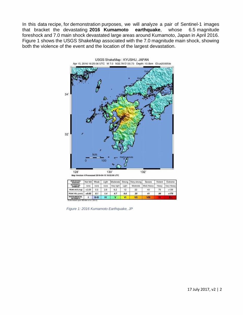
In this data recipe, for demonstration purposes, we will analyze a pair of Sentinel-1 images that bracket the devastating 2016 Kumamoto earthquake, whose 6.5 magnitude foreshock and 7.0 main shock devastated large areas around Kumamoto, Japan in April 2016. Figure 1 shows the USGS ShakeMap associated with the 7.0 magnitude main shock, showing both the violence of the event and the location of the largest devastation.

Figure 1: 2016 Kumamoto Earthquake, JP

17 July 2017, v2 | 3

2) A Word on Sentinel-1 Interferometric Wide Swath (IW) Data

The Interferometric Wide (IW) swath mode is the main acquisition mode over land for Sentinel-1. It acquires data with a 250km swath at 5m x 20m spatial resolution (single look). IW mode captures three sub-swaths using the Terrain Observation with Progressive Scans SAR (TOPSAR) acquisition principle.

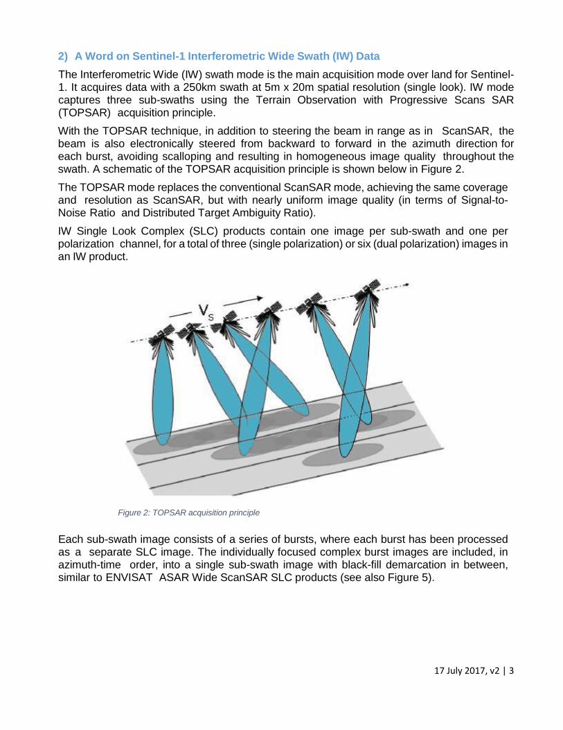
With the TOPSAR technique, in addition to steering the beam in range as in ScanSAR, the beam is also electronically steered from backward to forward in the azimuth direction for each burst, avoiding scalloping and resulting in homogeneous image quality throughout the swath. A schematic of the TOPSAR acquisition principle is shown below in Figure 2.

The TOPSAR mode replaces the conventional ScanSAR mode, achieving the same coverage and resolution as ScanSAR, but with nearly uniform image quality (in terms of Signal-to-Noise Ratio and Distributed Target Ambiguity Ratio).

IW Single Look Complex (SLC) products contain one image per sub-swath and one per polarization channel, for a total of three (single polarization) or six (dual polarization) images in an IW product.

Figure 2: TOPSAR acquisition principle

Each sub-swath image consists of a series of bursts, where each burst has been processed as a separate SLC image. The individually focused complex burst images are included, in azimuth-time order, into a single sub-swath image with black-fill demarcation in between, similar to ENVISAT ASAR Wide ScanSAR SLC products (see also Figure 5).

17 July 2017, v2 | 4

3) Sentinel-1 and the Kumamoto Earthquake

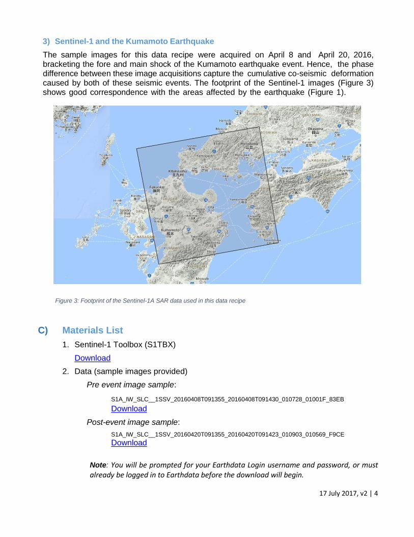
The sample images for this data recipe were acquired on April 8 and April 20, 2016, bracketing the fore and main shock of the Kumamoto earthquake event. Hence, the phase difference between these image acquisitions capture the cumulative co-seismic deformation caused by both of these seismic events. The footprint of the Sentinel-1 images (Figure 3) shows good correspondence with the areas affected by the earthquake (Figure 1).

Figure 3: Footprint of the Sentinel-1A SAR data used in this data recipe

C) Materials List

1. Sentinel-1 Toolbox (S1TBX)

Download

2. Data (sample images provided)

Pre event image sample:

S1A_IW_SLC__1SSV_20160408T091355_20160408T091430_010728_01001F_83EB

Download

Post-event image sample:

S1A_IW_SLC__1SSV_20160420T091355_20160420T091423_010903_010569_F9CE

Download

Note: You will be prompted for your Earthdata Login username and password, or must already be logged in to Earthdata before the download will begin.

17 July 2017, v2 | 5

D) Steps for InSAR Processing

Download software and data, and open data

Open data in S1TBX

Co-register the data

Interferogram formation and coherence

o Form the interferogram

o TOPS Deburst

o Topographic Phase Removal

o Multi-looking & Phase Filtering

o Geocoding & Export in a User-Defined Format

o Combine subswaths – optional Download Software & Data, and Open Data

1) Download materials

a. Download and install the S1TBX application (Select the correct version for your operating system)

b. Create a working folder for the Sentinel-1 sample images and intermediary

products created during processing

c. Download the sample images in Section C to the new working folder using ASF

Vertex, or use the download links provided

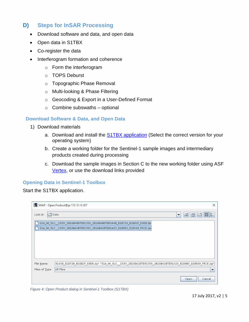
Opening Data in Sentinel-1 Toolbox

Start the S1TBX application.

Figure 4: Open Product dialog in Sentinel-1 Toolbox (S1TBX)

17 July 2017, v2 | 6

In order to perform interferometric processing, the input products should be two or more SLC products over the same area acquired at different times, such as the sample images provided in this tutorial.

1) Open the products – Step 1

Use the Open Product button in the top toolbar and browse for the location of the Sentinel-1 Interferometric Wide (IW) SLC products (Figure 4).

Note: Do not unzip the downloaded files.

Press and hold the <Ctrl> button and select the files. Click <Open> to load the files into S1TBX.

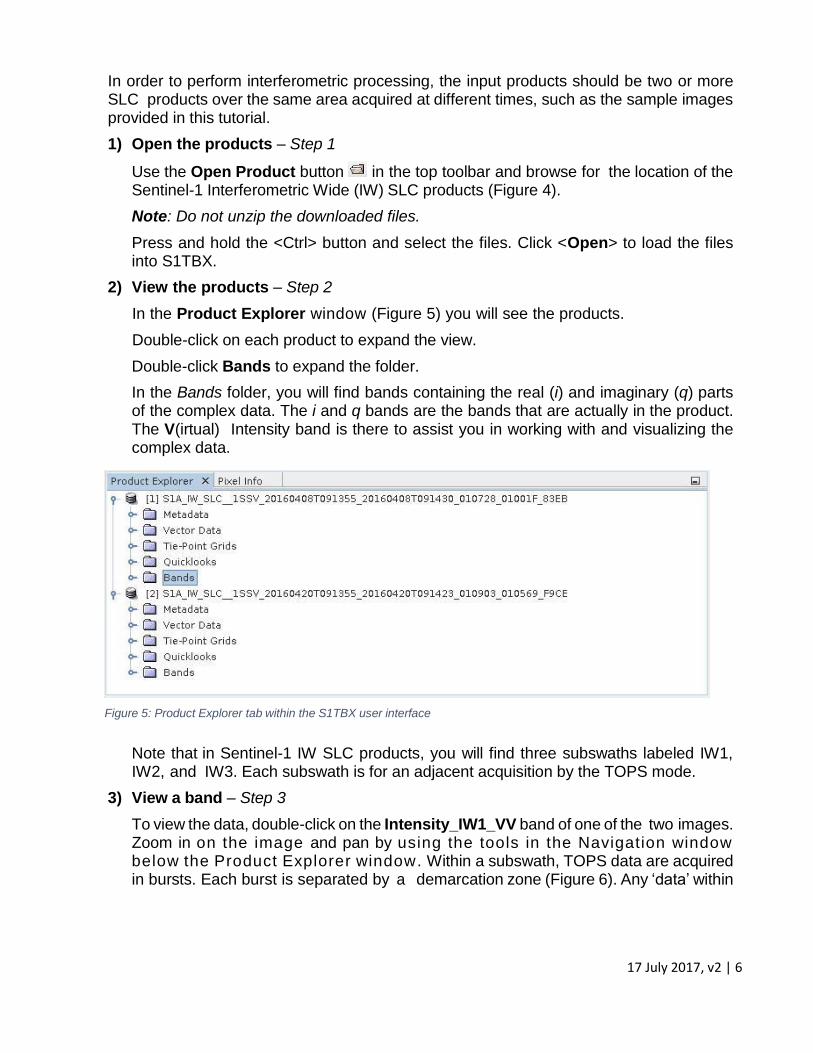
2) View the products – Step 2

In the Product Explorer window (Figure 5) you will see the products.

Double-click on each product to expand the view.

Double-click Bands to expand the folder.

In the Bands folder, you will find bands containing the real (i) and imaginary (q) parts of the complex data. The i and q bands are the bands that are actually in the product. The V(irtual) Intensity band is there to assist you in working with and visualizing the complex data.

Figure 5: Product Explorer tab within the S1TBX user interface

Note that in Sentinel-1 IW SLC products, you will find three subswaths labeled IW1, IW2, and IW3. Each subswath is for an adjacent acquisition by the TOPS mode.

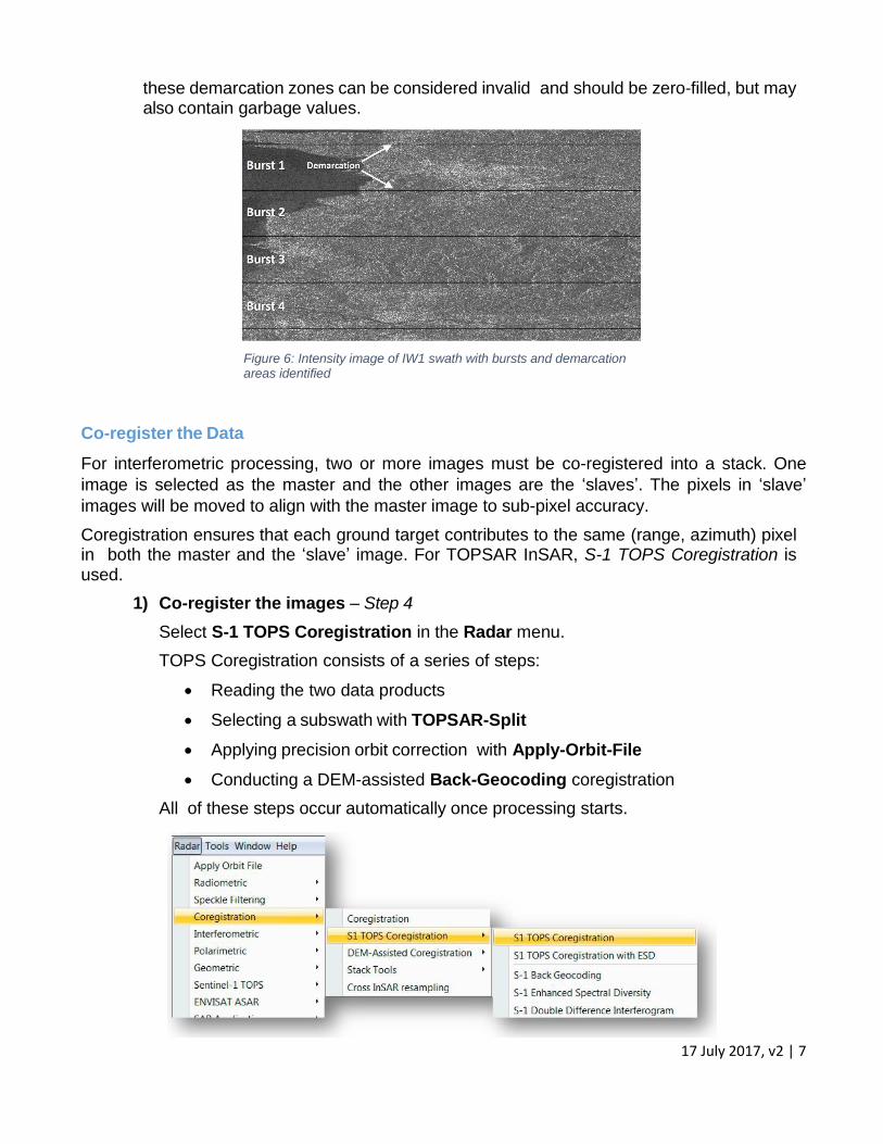
3) View a band – Step 3

To view the data, double-click on the Intensity_IW1_VV band of one of the two images. Zoom in on the image and pan by using the tools in the Navigation window below the Product Explorer window. Within a subswath, TOPS data are acquired in bursts. Each burst is separated by a demarcation zone (Figure 6). Any ‘data’ within

17 July 2017, v2 | 7

these demarcation zones can be considered invalid and should be zero-filled, but may also contain garbage values.

Figure 6: Intensity image of IW1 swath with bursts and demarcation areas identified

Co-register the Data

For interferometric processing, two or more images must be co-registered into a stack. One

image is selected as the master and the other images are the ‘slaves’. The pixels in ‘slave’

images will be moved to align with the master image to sub-pixel accuracy.

Coregistration ensures that each ground target contributes to the same (range, azimuth) pixel in both the master and the ‘slave’ image. For TOPSAR InSAR, S-1 TOPS Coregistration is used.

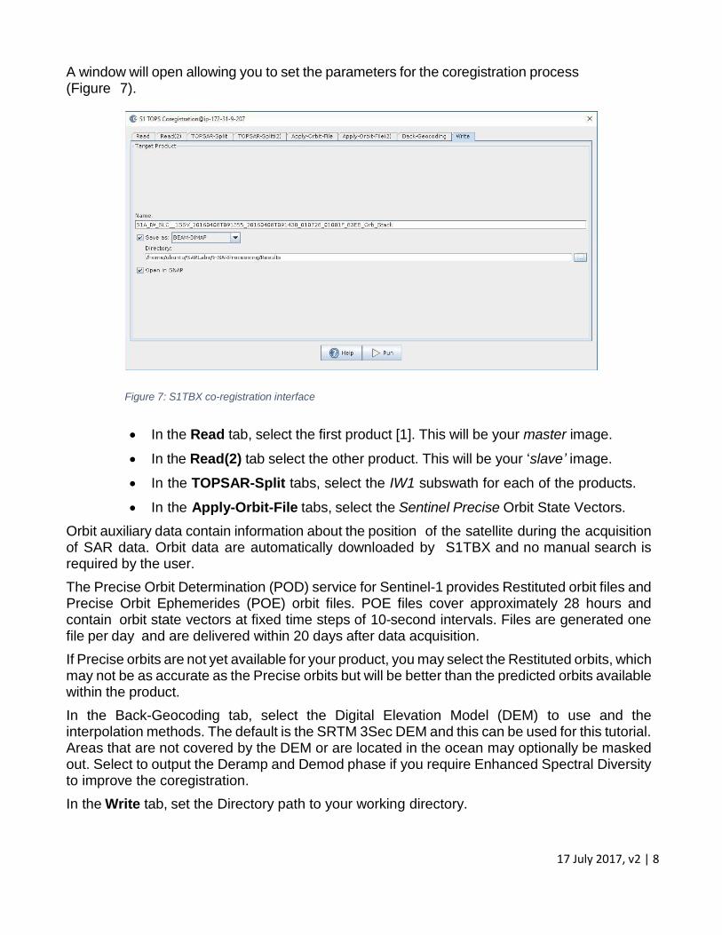
1) Co-register the images – Step 4

Select S-1 TOPS Coregistration in the Radar menu.

TOPS Coregistration consists of a series of steps:

Reading the two data products

Selecting a subswath with TOPSAR-Split

Applying precision orbit correction with Apply-Orbit-File

Conducting a DEM-assisted Back-Geocoding coregistration

All of these steps occur automatically once processing starts.

17 July 2017, v2 | 8

A window will open allowing you to set the parameters for the coregistration process (Figure 7).

Figure 7: S1TBX co-registration interface

In the Read tab, select the first product [1]. This will be your master image.

In the Read(2) tab select the other product. This will be your ‘slave’ image.

In the TOPSAR-Split tabs, select the IW1 subswath for each of the products.

In the Apply-Orbit-File tabs, select the Sentinel Precise Orbit State Vectors.

Orbit auxiliary data contain information about the position of the satellite during the acquisition of SAR data. Orbit data are automatically downloaded by S1TBX and no manual search is required by the user.

The Precise Orbit Determination (POD) service for Sentinel-1 provides Restituted orbit files and Precise Orbit Ephemerides (POE) orbit files. POE files cover approximately 28 hours and contain orbit state vectors at fixed time steps of 10-second intervals. Files are generated one file per day and are delivered within 20 days after data acquisition.

If Precise orbits are not yet available for your product, you may select the Restituted orbits, which may not be as accurate as the Precise orbits but will be better than the predicted orbits available within the product.

In the Back-Geocoding tab, select the Digital Elevation Model (DEM) to use and the interpolation methods. The default is the SRTM 3Sec DEM and this can be used for this tutorial. Areas that are not covered by the DEM or are located in the ocean may optionally be masked out. Select to output the Deramp and Demod phase if you require Enhanced Spectral Diversity to improve the coregistration.

In the Write tab, set the Directory path to your working directory.

17 July 2017, v2 | 9

Click <Run> to begin co-registering the data. The resulting coregistered stack product will appear in the Product Explorer window with the suffix Orb_Stack.

Interferogram Formation & Coherence Estimation

The interferogram is formed by cross-multiplying the master image with the complex conjugate of the ‘ slave’. The amplitude of both images is multiplied while their respective phases are differenced to form the interferogram.

The phase difference map, i.e., interferometric phase at each SAR image pixel depends only on the difference in the travel paths from each of the two SARs to the considered resolution cell.

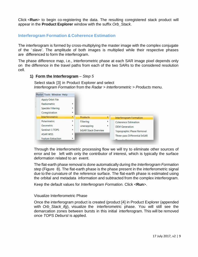
1) Form the Interferogram – Step 5

Select stack [3] in Product Explorer and select Interferogram Formation from the Radar > Interferometric > Products menu.

Through the interferometric processing flow we will try to eliminate other sources of error and be left with only the contributor of interest, which is typically the surface deformation related to an event.

The flat-earth phase removal is done automatically during the Interferogram Formation step (Figure 8). The flat-earth phase is the phase present in the interferometric signal due to the curvature of the reference surface. The flat-earth phase is estimated using the orbital and metadata information and subtracted from the complex interferogram.

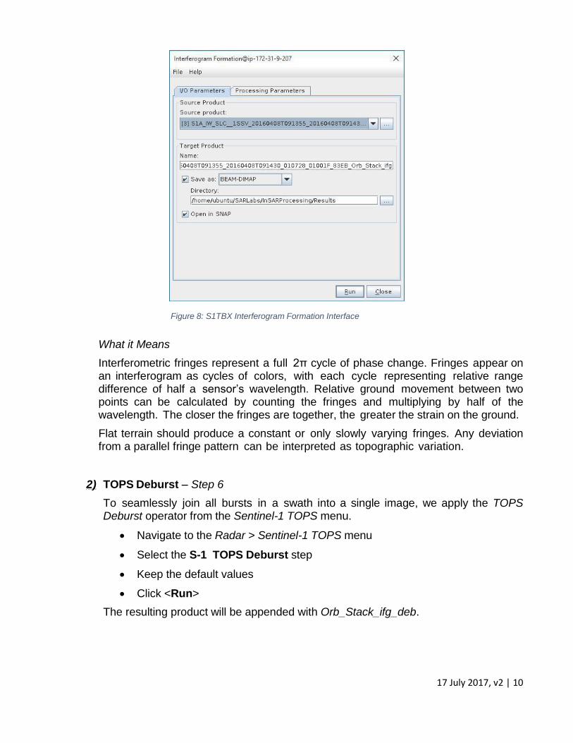
Keep the default values for Interferogram Formation. Click <Run>.

Visualize Interferometric Phase

Once the interferogram product is created (product [4] in Product Explorer (appended with Orb_Stack_ifg), visualize the interferometric phase. You will still see the demarcation zones between bursts in this initial interferogram. This will be removed once TOPS Deburst is applied.

17 July 2017, v2 | 10

Figure 8: S1TBX Interferogram Formation Interface

What it Means

Interferometric fringes represent a full 2π cycle of phase change. Fringes appear on an interferogram as cycles of colors, with each cycle representing relative range difference of half a sensor’s wavelength. Relative ground movement between two points can be calculated by counting the fringes and multiplying by half of the wavelength. The closer the fringes are together, the greater the strain on the ground.

Flat terrain should produce a constant or only slowly varying fringes. Any deviation from a parallel fringe pattern can be interpreted as topographic variation.

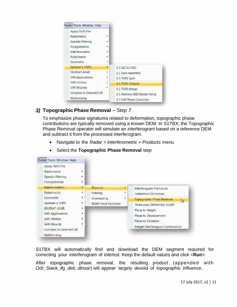
2) TOPS Deburst – Step 6

To seamlessly join all bursts in a swath into a single image, we apply the TOPS Deburst operator from the Sentinel-1 TOPS menu.

Navigate to the Radar > Sentinel-1 TOPS menu

Select the S-1 TOPS Deburst step

Keep the default values

Click <Run>

The resulting product will be appended with Orb_Stack_ifg_deb.

17 July 2017, v2 | 11

3) Topographic Phase Removal – Step 7

To emphasize phase signatures related to deformation, topographic phase contributions are typically removed using a known DEM. In S1TBX, the Topographic Phase Removal operator will simulate an interferogram based on a reference DEM and subtract it from the processed interferogram.

Navigate to the Radar > Interferometric > Products menu

Select the Topographic Phase Removal step

S1TBX will automatically find and download the DEM segment required for correcting your interferogram of interest. Keep the default values and click <Run>.

After topographic phase removal, the resulting product (appended with Orb_Stack_ifg_deb_dinsar) will appear largely devoid of topographic influence.

17 July 2017, v2 | 12

Multi-looking & Phase Filtering

You will see that up to this stage, your interferogram looks very noisy and fringe patterns are difficult to discern. Hence, we will apply two subsequent processing steps to reduce noise and enhance the appearance of the deformation fringes.

Interferometric phase can be corrupted by noise from:

Temporal decorrelation

Geometric decorrelation

Volume scattering

Processing error

To be able to properly analyze the phase signatures in the interferogram, the signal-to-noise ratio will be increased by applying multi-looking and phase filtering techniques:

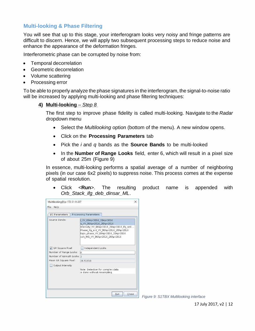
4) Multi-looking – Step 8

The first step to improve phase fidelity is called multi-looking. Navigate to the Radar dropdown menu

Select the Multilooking option (bottom of the menu). A new window opens.

Click on the Processing Parameters tab

Pick the i and q bands as the Source Bands to be multi-looked

In the Number of Range Looks field, enter 6, which will result in a pixel size of about 25m (Figure 9)

In essence, multi-looking performs a spatial average of a number of neighboring pixels (in our case 6x2 pixels) to suppress noise. This process comes at the expense of spatial resolution.

Click <Run>. The resulting product name is appended with Orb_Stack_ifg_deb_dinsar_ML.

Figure 9: S1TBX Multilooking interface

17 July 2017, v2 | 13

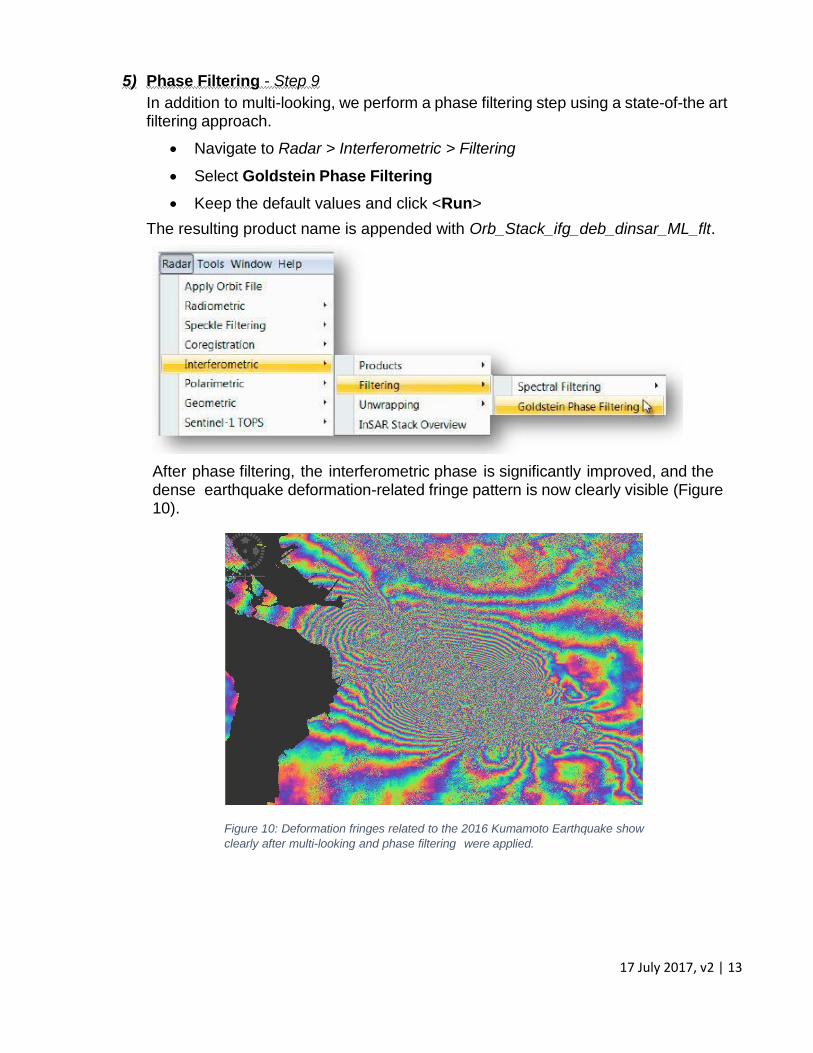
5) Phase Filtering - Step 9

In addition to multi-looking, we perform a phase filtering step using a state-of-the art filtering approach.

Navigate to Radar > Interferometric > Filtering

Select Goldstein Phase Filtering

Keep the default values and click <Run>

The resulting product name is appended with Orb_Stack_ifg_deb_dinsar_ML_flt.

After phase filtering, the interferometric phase is significantly improved, and the dense earthquake deformation-related fringe pattern is now clearly visible (Figure 10).

Figure 10: Deformation fringes related to the 2016 Kumamoto Earthquake show

clearly after multi-looking and phase filtering were applied.

17 July 2017, v2 | 14

Geocoding & Export in a User-defined Format

To make the data useful to geoscientists, the interferometric phase image needs to be projected into a geographic coordinate system using a DEM-assisted geocoding step.

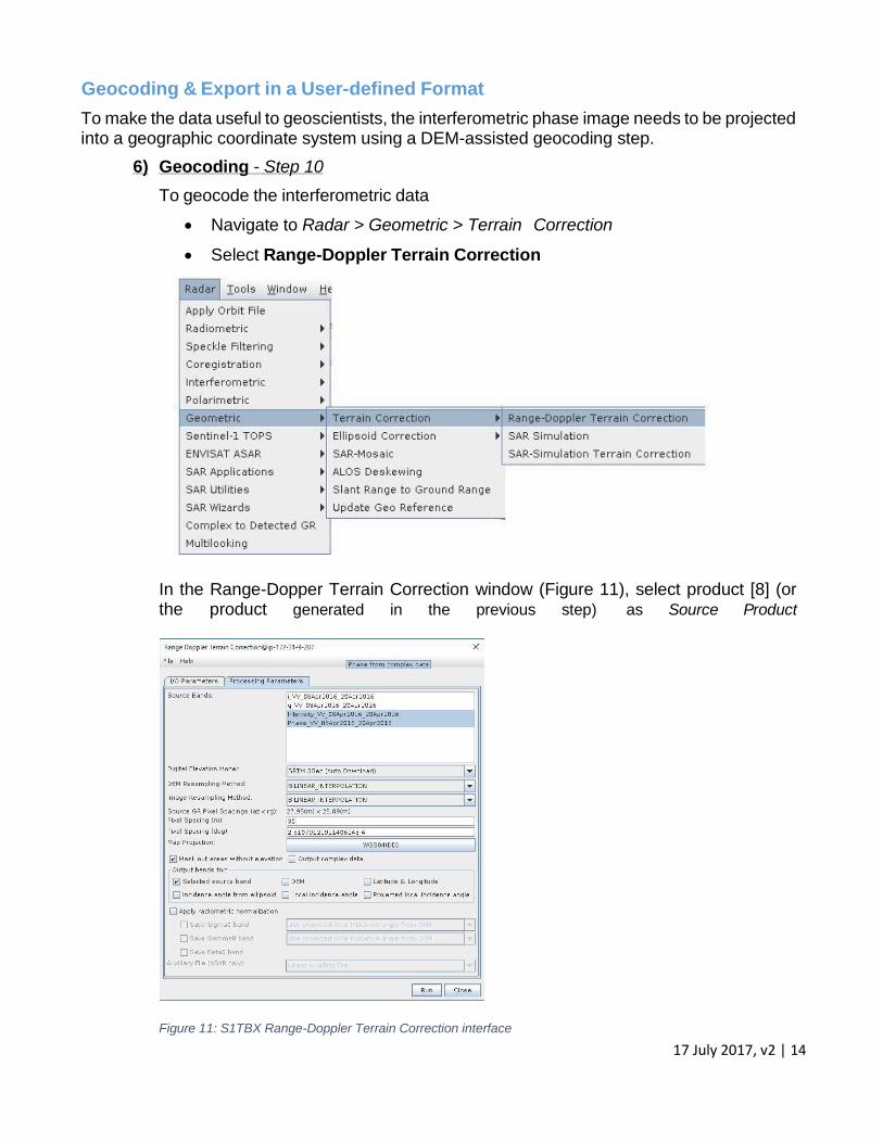
6) Geocoding - Step 10

To geocode the interferometric data

Navigate to Radar > Geometric > Terrain Correction

Select Range-Doppler Terrain Correction

In the Range-Dopper Terrain Correction window (Figure 11), select product [8] (or the product generated in the previous step) as Source Product

Figure 11: S1TBX Range-Doppler Terrain Correction interface

17 July 2017, v2 | 15

In Processing Parameters

Select the Intensity and Phase images as Source Bands to be geocoded

Adjust the pixel spacing if you want (e.g., 30m)

Click <Run>

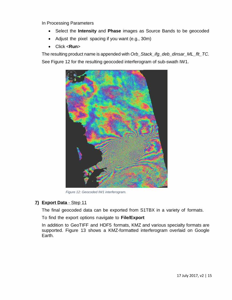
The resulting product name is appended with Orb_Stack_ifg_deb_dinsar_ML_flt_TC.

See Figure 12 for the resulting geocoded interferogram of sub-swath IW1.

Figure 12: Geocoded IW1 interferogram.

7) Export Data - Step 11

The final geocoded data can be exported from S1TBX in a variety of formats.

To find the export options navigate to File/Export

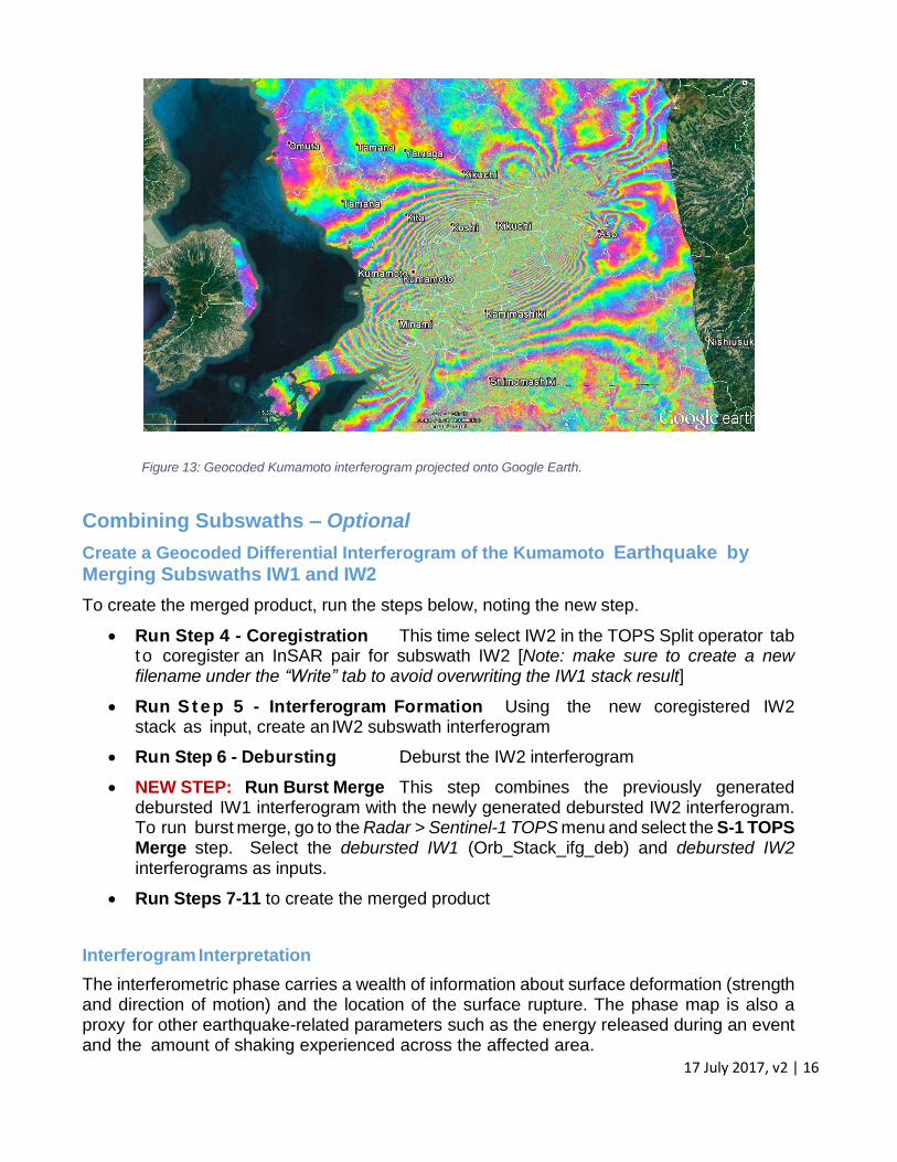
In addition to GeoTIFF and HDF5 formats, KMZ and various specialty formats are supported. Figure 13 shows a KMZ-formatted interferogram overlaid on Google Earth.

17 July 2017, v2 | 16

Figure 13: Geocoded Kumamoto interferogram projected onto Google Earth.

Combining Subswaths – Optional

Create a Geocoded Differential Interferogram of the Kumamoto Earthquake by Merging Subswaths IW1 and IW2

To create the merged product, run the steps below, noting the new step.

Ru n Step 4 - Cor egi stration This time select IW2 in the TOPS Split operator tab to coregister an InSAR pair for subswath IW2 [Note: make sure to create a new filename under the “Write” tab to avoid overwriting the IW1 stack result]

Ru n S t e p 5 - In ter f erogr am Fo r mati on Using the new coregistered IW2 stack as input, create an IW2 subswath interferogram

Ru n Step 6 - Deb ur stin g Deburst the IW2 interferogram

NEW STEP: Run Burst Merge This step combines the previously generated debursted IW1 interferogram with the newly generated debursted IW2 interferogram. To run burst merge, go to the Radar > Sentinel-1 TOPS menu and select the S-1 TOPS Merge step. Select the debursted IW1 (Orb_Stack_ifg_deb) and debursted IW2 interferograms as inputs.

Run Steps 7-11 to create the merged product

Interferogram Interpretation

The interferometric phase carries a wealth of information about surface deformation (strength and direction of motion) and the location of the surface rupture. The phase map is also a proxy for other earthquake-related parameters such as the energy released during an event and the amount of shaking experienced across the affected area.

17 July 2017, v2 | 17

E) InSAR Extended Reading List

Summary Articles about SAR:

Moreira, A., Prats-Iraola, P., Younis, M., Krieger, G., Hajnsek, I., & Papathanassiou, K. P. (2013). A tutorial on synthetic aperture radar. IEEE Geoscience and Remote Sensing Magazine, 1(1), 6-43.

Rosen, P. A., Hensley, S., Joughin, I. R., Li, F. K., Madsen, S. N., Rodriguez, E., & Goldstein, R. M. (2000). Synthetic aperture radar interferometry. Proceedings of the IEEE, 88(3), 333-382.

Bamler, R., & Hartl, P. (1998). Synthetic aperture radar interferometry. Inverse problems, 14(4), R1.

Bürgmann, R., Rosen, P. A., & Fielding, E. J. (2000). Synthetic aperture radar interferometry to measure Earth’s surface topography and its deformation. Annual review of earth and planetary sciences, 28(1), 169-209.

Simons, M., and P. A. Rosen (2007), Interferometric synthetic aperture radar geodesy, in Geodesy, Treatise on Geophysics, vol. 3, edited by T. Herring, pp. 391–446, Elsevier.

Interesting Articles by Topic:

InSAR Processing

Rosen, P. A., Hensley, S., Joughin, I. R., Li, F. K., Madsen, S. N., Rodriguez, E., & Goldstein, R. M. (2000). Synthetic aperture radar interferometry. Proceedings of the IEEE, 88(3), 333-382.

Bamler, R., & Hartl, P. (1998). Synthetic aperture radar interferometry. Inverse problems, 14(4), R1.

Bürgmann, R., Rosen, P. A., & Fielding, E. J. (2000). Synthetic aperture radar

interferometry to measure Earth’s surface topography and its deformation. Annual review of earth and planetary sciences, 28(1), 169-209.

Volcanic Source Modeling Using InSAR

Mogi, K. (1958), Relations between the eruptions of various volcanoes and the deformations of the ground surfaces around them, Bull. Earthquake Research Inst., 36, 99–134.

Lohman, R. B., & Simons, M. (2005). Some thoughts on the use of InSAR data to constrain models of surface deformation: Noise structure and data downsampling. Geochemistry, Geophysics, Geosystems, 6(1).

Lu, Z. (2007). InSAR imaging of volcanic deformation over cloud-prone areas–Aleutian Islands. Photogrammetric Engineering & Remote Sensing, 73(3), 245-257.

17 July 2017, v2 | 18

Lu, Z., & Dzurisin, D. (2010). Ground surface deformation patterns, magma supply, and magma storage at Okmok volcano, Alaska, from InSAR analysis: 2. Coeruptive deflation, July–August 2008. Journal of Geophysical Research: Solid Earth, 115(B5).

Lu, Z., Masterlark, T., & Dzurisin, D. (2005). Interferometric synthetic aperture radar study of Okmok volcano, Alaska, 1992–2003: Magma supply dynamics and postemplacement lava flow deformation. Journal of Geophysical Research: Solid Earth, 110(B2).

Baker, S., & Amelung, F. (2012). Top‐down inflation and deflation at the summit

of Kīlauea Volcano, Hawai ‘i observed with InSAR. Journal of Geophysical Research: Solid Earth, 117(B12).

Wright, T. J., Lu, Z., & Wicks, C. (2003). Source model for the Mw 6.7, 23 October 2002, Nenana Mountain Earthquake (Alaska) from InSAR. Geophysical Research Letters, 30(18). [Supplements]

InSAR Time Series Analysis

Ferretti, A., Prati, C., & Rocca, F. (2001). Permanent scatterers in SAR interferometry. IEEE Transactions on geoscience and remote sensing, 39(1), 8-20.

Berardino, P., Fornaro, G., Lanari, R., & Sansosti, E. (2002). A new algorithm for surface deformation monitoring based on small baseline differential SAR interferograms. IEEE Transactions on Geoscience and Remote Sensing, 40(11), 2375-2383.

Lanari, R., Mora, O., Manunta, M., Mallorquí, J. J., Berardino, P., & Sansosti, E. (2004). A small-baseline approach for investigating deformations on full-resolution differential SAR interferograms. IEEE Transactions on Geoscience and Remote Sensing, 42(7), 1377-1386.

Hooper, A., Segall, P., & Zebker, H. (2007). Persistent scatterer interferometric synthetic aperture radar for crustal deformation analysis, with application to Volcán Alcedo, Galápagos. Journal of Geophysical Research: Solid Earth, 112(B7).

Ferretti, A., Fumagalli, A., Novali, F., Prati, C., Rocca, F., & Rucci, A. (2011). A new algorithm for processing interferometric data-stacks: SqueeSAR. IEEE Transactions on Geoscience and Remote Sensing, 49(9), 3460-3470.