SENSOR STABILIZATION, LOCALIZATION, OBSTACLE DETECTION,

AND PATH PLANNING FOR AUTONOMOUS ROVERS:

A CASE STUDY

by

ANDREW AUBREY FAULKNER

KENNETH G. RICKS, COMMITTEE CHAIR

DAVID J. JACKSON

MONICA D. ANDERSON

A THESIS

Submitted in partial fulfillment of the requirements

for the degree of Master of Science

in the Department of Electrical and Computer Engineering

In the Graduate School of

The University of Alabama

TUSCALOOSA, ALABAMA

2015

Copyright Andrew Aubrey Faulkner 2015

ALL RIGHTS RESERVE

ii

ABSTRACT

Autonomous rovers are the next step in exploration of terrestrial planets. Current rovers

contain some forms of semi-autonomy, but many functions are still performed by remote human

operators. As the distance between Earth and the exploration target increases, communication

delays will make teleoperation of rover platforms increasingly difficult. Through the use of

autonomous systems, operators may give mission parameters to autonomous exploration rovers

and allow onboard systems to carry out the task. In addition, if future exploration requires a

repetitive task, such as resource gathering, autonomous rovers represent the best technology for

the job. Autonomous rovers face many challenges. Among them are sensor stabilization,

localization, obstacle detection, and path planning.

This thesis describes an approach for each of the above mentioned challenges. Sensor

stabilization was performed using an inertial measurement unit (IMU) and the reverse angle

method of stabilization. A 2D Light Detection and Ranging (LIDAR) sensor provided input data

for a landmark-based localization algorithm. The same LIDAR unit was actuated to perform 3D

scans used in an obstacle detection method based upon ground plane removal, via random

sample consensus (RANSAC), and Euclidean Clustering. A modified A* algorithm was used as

an occupancy grid-based path planner. The approaches were verified through implementation on

the University of Alabama Modular Autonomous Robotic Terrestrial Explorer (MARTE)

platform as part of the 2014 NASA Robotic Mining Competition.

iii

LIST OF ABBREVIATIONS AND SYMBOLS

AHRS Attitude and Heading Reference System

DCM Direct Cosine Matrix

GPS Global Positioning System

IMU Inertial Measurement Unit

IR Infrared

LIDAR Light Detection and Ranging

MARTE Modular Autonomous Robotic Terrestrial Explorer

MEMS Microelectromechanical Systems

NASA National Aeronautics and Space Administration

RANSAC Random Sample Consensus

RMC Robotic Mining Competition

SASS Sensor Active Stabilization System

SLAM Simultaneous Localization and Mapping

iv

ACKNOWLEDGEMENTS

I would like to thank the members of the University of Alabama Astrobotics team who

were instrumental in the implementation and testing of MARTE: Caleb Leslie as Team Lead,

Michael Carswell as Base Subsystem Lead, Kellen Schroeter as Module Subsystem Lead, David

Sandel as Software Team Co-lead, and the other members of the Astrobotics team. I would like

to give special mention to Derrill Koelz and Mitchell Spryn who were instrumental members of

the Software Team. I’d like to thank my committee members, Dr. Jackson and Dr. Anderson, for

their knowledge and support throughout my academic years. Finally, I would like to thank Dr.

Kenneth Ricks for his support through many years as an advisor, professor, supervisor, and

friend.

This paper is dedicated to my parents. Thank you for supporting me in all of my pursuits.

v

CONTENTS

ABSTRACT .................................................................................................................................... ii

LIST OF ABBREVIATIONS AND SYMBOLS .......................................................................... iii

ACKNOWLEDGEMENTS ........................................................................................................... iv

LIST OF TABLES ........................................................................................................................ vii

LIST OF FIGURES ..................................................................................................................... viii

1. PROBLEM STATEMENT ......................................................................................................... 1

1.1 Introduction .......................................................................................................................... 1

1.2 Case Study ............................................................................................................................ 2

2. SENSOR STABILIZATION ...................................................................................................... 6

2.1 Types of Sensor Stabilization ............................................................................................... 6

2.2 Frame Transforms ................................................................................................................ 8

2.3 Case Study Implementation ............................................................................................... 10

2.3.1 AHRS........................................................................................................................ 11

2.3.2 SASS ......................................................................................................................... 14

2.4 Active Stabilization Testing ............................................................................................... 14

3. LOCALIZATION ..................................................................................................................... 18

3.1 Localization Approaches .................................................................................................... 18

3.2 Case Study .......................................................................................................................... 21

3.3 Testing ................................................................................................................................ 26

4. OBSTACLE DETECTION ...................................................................................................... 28

4.1 Obstacle Detection Algorithms .......................................................................................... 28

vi

4.2 Case Study .......................................................................................................................... 29

4.3 Testing ................................................................................................................................ 34

5. PATH PLANNING .................................................................................................................. 36

5.1 Path Planning Algorithms .................................................................................................. 36

5.2 Case Study .......................................................................................................................... 37

6. SYSTEM TESTING ................................................................................................................. 47

7. CONCLUSIONS AND FUTURE WORK ............................................................................... 50

REFERENCES ............................................................................................................................. 52

vii

LIST OF TABLES

6.1 RMC Run Results ............................................................................................................................ 48

6.2 Execution Times for Individual Elements ................................................................................... 49

viii

LIST OF FIGURES

1.1 Autonomous Rover Navigation Challenges........................................................................... 2

1.2 RMC Operation Environment ................................................................................................ 4

1.3 SolidWorks Model of UA Entry ............................................................................................ 5

2.1 Example of the Need for Stabilization ................................................................................... 7

2.2 Frame Transforms .................................................................................................................. 9

2.3 Accuracy Requirement......................................................................................................... 15

2.4 Average Absolute Error Across All Runs ............................................................................ 16

2.5 Sample Run Error ................................................................................................................ 17

3.1 Trinagulation Illustration ..................................................................................................... 20

3.2 2D Scan of Environment Landmarks ................................................................................... 23

3.3 Line Extraction Performed on 2D Scan ............................................................................... 24

3.4 Possible Localization Transforms ........................................................................................ 25

3.5 Average Error for Localization Testing ............................................................................... 26

4.1 Example Obstacle Zone ....................................................................................................... 30

4.2 Pointcloud of Obstacle Zone with Obstacles Highlighted ................................................... 31

4.3 Data is Divided into Smaller Local Pointclouds .................................................................. 32

4.4 Occupancy Grid of Example Obstacle Zone ....................................................................... 34

4.5 Obstacle Detection Testing Results ..................................................................................... 35

5.1 A* Example Initial Conditions ............................................................................................ 39

5.2 Results of Iteration 1 ............................................................................................................ 40

ix

5.3 Results of Iteration 2 ............................................................................................................ 40

5.4 Results of Iteration 3 ............................................................................................................ 41

5.5 Results of Iteration 4 ............................................................................................................ 41

5.6 Results of Iteration 5 ............................................................................................................ 42

5.7 Forward Grid of Figure 4.4 .................................................................................................. 44

5.8 Full Path Returned by Modified A*..................................................................................... 45

5.9 Post-processing Produced Path ............................................................................................ 46

1

CHAPTER 1

PROBLEM STATEMENT

1.1 Introduction

With the increased focus placed on inter-planetary exploration for space agencies around

the world, the use of autonomous or semi-autonomous rover platforms has increased [1]. The

communication delay between Earth and Mars averages twenty minutes [2]. This makes human

piloted rovers inefficient and human resource dependent [3]. Any problems encountered by the

rover will not be discovered by the operating crew until after the communication time delay has

passed. Efficient exploration and navigation of the complex terrain found on terrestrial planets

requires autonomous navigation using onboard processing. Autonomous rovers can traverse

terrain at reduced speeds but with substantially decreased delays between movement commands

so long as the processing for the autonomous system is accomplished onsite. The goal of

autonomous terrestrial rovers is to process all information necessary for navigation onboard to

eliminate the possibility of communication interruption and to allow for efficient operation.

Autonomous rover navigation involves the ability of a platform to sense its environment,

plan operations to achieve goals within this environment, and safely carry out these operations. A

non-exhaustive list of the challenges faced by terrestrial rovers includes: sensor stabilization,

localization, obstacle detection, and path planning [3]. These problems are interrelated as

represented by the flowchart in Figure 1.1.

2

Figure 1.1: Autonomous Rover Navigation Challenges

Sensor stabilization involves the proper alignment of sensors with respect to either the

robot or its environment. This is the first challenge, and any errors made during this step

propagate to all other aspects of autonomous rover navigation that involve the sensors under

stabilization. Localization is the ability for the rover to know its location within its environment.

This localization information is often with reference to a known location within the environment

such as a landing or collection site. Obstacle detection involves the collection and interpretation

of data representing the rover’s operational environment. Objects or terrain that present

operational hazards to the rover are identified and marked as areas to be avoided if possible. Path

planning formulates the movement strategy from its current location to an operational goal.

Decisions are made with respect to the rover’s operational kinematics as well as the knowledge

of the environment provided by the obstacle detection [3], [4].

1.2 Case Study

The challenges presented above must be faced in many autonomous rover applications. In

order to provide operational details, each of the challenges mentioned is discussed with respect

to a case study undertaken at The University of Alabama for the purpose of competing in the

Fifth Annual NASA Robotic Mining Competition (RMC). The challenge presented to the teams

competing in the competition is to “design and build a mining robot that can traverse the

Sensor Stabilization

Localization

Obstacle Detection

Path Planning

3

simulated Martian chaotic terrain and excavate Martian regolith” [5]. Fifty universities presented

their designs to NASA and industry judges in May 2014 at the Kennedy Space Center in Cape

Canaveral, Florida. Teams consisted of combinations of graduate and undergraduate students.

Trials of each design are conducted within a simulated Martian environment provided by

NASA. A breakdown of the operational environment can be seen in Figure 1.2. At the beginning

of each competition run, NASA randomly selects the starting position within the marked starting

area. In addition, the orientation of the rover is randomly selected to be one of the four cardinal

directions. A series of obstacles consisting of rocks and craters is created within the central zone

of the environment. The last portion of the environment is the designated mining area. Regolith

may only be excavated from this area of the operational environment. Once the regolith is

collected, it must be transported back across the obstacle zone and deposited within a collection

bin outside the starting zone. Operators and observers for each team are stationed in a remote

command center away from the simulated environment. Teams are given two ten-minute runs

within the environment with differing starting poses and obstacle layouts. Points are awarded

based upon the amount of regolith deposited within the collection bin and for varying thresholds

of autonomous or semi-autonomous operation. Points are deducted for the mass of the rover and

any communication bandwidth used to correspond with operators or observers within the

command center.

4

Figure 1.2: RMC Operation Environment [5]

The rover constructed for entry into the RMC is a modular operational platform. The base

consisted of the drive train, drive electronics, central onboard communication, and power supply

for the platform. Upon this base can be placed any number of task specific modules that fit a

predesigned footprint and a specified electrical interface [6]. This allows for the same rover to

perform a variety of operational procedures based upon the operational module placed upon it.

The module in use is a bucket chain excavator designed to mine the regolith found in the

simulated Martian environment. A SolidWorks model of the platform can be seen in Figure 1.3.

In addition to physical modularity, the electronics for autonomous operation are housed in a

separate enclosure from the drive electronics. This allows for the quick and easy removal of the

autonomous system while leaving all electronics onboard necessary for manual control and

operation.

5

Figure 1.3: SolidWorks Model of UA Entry

Each of the challenges mentioned in Section 1.1 are addressed within the case study. An

active sensor stabilization platform is used to actuate a LIDAR. The LIDAR is multiplexed for

use in both localization and obstacle detection. Localization is accomplished through the use of

an a priori map and a 2D scan of the boundaries of the environment. The boundaries are treated

as landmarks and the pose of the rover is calculated. For obstacle detection, the LIDAR is

actuated to create a 3D pointcloud of the environment used in path planning. The pointcloud is

then interpreted using RANSAC and Euclidean Clustering to provide the location of both

concave and convex obstacles. All of this information is then input into a path planning

algorithm based upon the A* graph traversal algorithm which computes a safe operational path

for the rover to follow. All computation required by the autonomous navigation of the platform is

performed by the onboard electronics and a minimal amount of data necessary for observation is

transmitted to the operational command center.

6

CHAPTER 2

SENSOR STABILIZATION

2.1 Types of Sensor Stabilization

Sensor stabilization is the first challenge present in autonomous rover navigation and has

evolved much over the history of robotics [7]. The accuracy of the stabilization affects all further

use of the information from the stabilized sensor [8]. While sensor stabilization is important for

many types of sensors, it is extremely vital in the use of narrow field sensors such as LIDAR,

ultrasonic, and IR sensors. Since each of these sensors has a narrow beam width, they are more

prominently affected by changes in position. This effect is magnified at greater distances. An

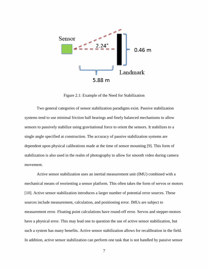
example of a narrow beam sensor can be visualized in Figure 2.1. In this example, a narrow

beam sensor is placed on a platform 5.88 m away from a landmark that is 0.46 m high. If the

sensor is placed 0.23 m above the ground and the terrain is entirely flat, then it will manage to

detect the landmark. However, if the same sensor is statically mounted to a rover frame that is

inclined a mere 2.24° then the sensor will miss the landmark. This increment of incline is

minimal compared to the incline generated when a platform encounters small craters, rocks, and

undulations in terrain, such as those found in the RMC. As is illustrated by the example,

statically mounting sensors to a rover chassis is not a viable solution in autonomous rover

navigation.

7

Figure 2.1: Example of the Need for Stabilization

Two general categories of sensor stabilization paradigms exist. Passive stabilization

systems tend to use minimal friction ball bearings and finely balanced mechanisms to allow

sensors to passively stabilize using gravitational force to orient the sensors. It stabilizes to a

single angle specified at construction. The accuracy of passive stabilization systems are

dependent upon physical calibrations made at the time of sensor mounting [9]. This form of

stabilization is also used in the realm of photography to allow for smooth video during camera

movement.

Active sensor stabilization uses an inertial measurement unit (IMU) combined with a

mechanical means of reorienting a sensor platform. This often takes the form of servos or motors

[10]. Active sensor stabilization introduces a larger number of potential error sources. These

sources include measurement, calculation, and positioning error. IMUs are subject to

measurement error. Floating point calculations have round-off error. Servos and stepper-motors

have a physical error. This may lead one to question the use of active sensor stabilization, but

such a system has many benefits. Active sensor stabilization allows for recalibration in the field.

In addition, active sensor stabilization can perform one task that is not handled by passive sensor

8

stabilization, the ability to dynamically determine the angle at which the sensor should be

stabilized at runtime. It also allows for multiplexing use of the sensor for purposes that require

different angles of inclination.

Previous work in the area of two axis sensor stabilization is immense. Inertial

stabilization has been implemented using a wide variety of technology ranging from the MEMS

gyroscope to the fiber optic gyroscope used in military grade applications [7]. The stabilization

system implemented in the case study uses an IMU that contains MEMS gyroscopes. This

technology is lightweight and relatively inexpensive making it perfect for hobby and prototype

grade implementations. Vehicle attitude can be interchangeably represented in a variety of

rotation matrices: quaternions, Euler angles, and direct cosine matrices [11]. The system is an

indirect line of sight stabilization system in that the IMU is mounted upon the robot frame

instead of the stabilization mechanism. This requires an additional coordinate transform to be

performed between the vehicle and stabilization mechanism coordinate frames [12]. The control

algorithm for the mechanical operation is the inverse angle control method, a computationally

efficient control method.

2.2 Frame Transforms

One of the key concepts involved in active sensor stabilization is frame transforms. The

IMU measures the roll, pitch, and yaw within the robot frame, or how it appears to the rover.

Often one wants to translate these angular offsets into the global frame to align them with an

absolute source like gravity. The global frame can be described using three orthonormal vectors

within the frame.

𝐼𝐺 = {1,0,0}𝑇 (1)

9

𝐽𝐺 = {0,1,0}𝑇 (2)

𝐾𝐺 = {0,0,1}𝑇 (3)

Likewise the robot frame can be described as three orthonormal vectors within its frame space,

as shown in Figure 2.2.

𝑖𝑅 = {1,0,0}𝑇 (4)

𝑗𝑅 = {0,1,0}𝑇 (5)

𝑘𝑅 = {0,0,1}𝑇 (6)

Figure 2.2: Frame Transforms [13]

The vectors that describe the robot frame can be described in terms of the global frame vectors.

This is done by determining the length of the projection of the robot frame vectors onto the

global coordinate frame.

𝑖𝐺 = {𝑖𝑥𝐺 , 𝑖𝑦

𝐺 , 𝑖𝑧𝐺}

𝑇 (7)

𝑗𝐺 = {𝑗𝑥𝐺 , 𝑗𝑦

𝐺 , 𝑗𝑧𝐺}

𝑇 (8)

𝑘𝐺 = {𝑘𝑥𝐺 , 𝑘𝑦

𝐺 , 𝑘𝑧𝐺}

𝑇 (9)

10

The individual components of the projections are calculated as shown in (10) where I,i is the

angle between the I vector in the global frame and the i vector in the robot frame.

𝑖𝑥𝐺 = cos(𝐼, 𝑖) = 𝐼.𝑖 (10)

Since both the I and i vectors are unit vectors, taking the cosine of the angle between them is

equivalent to computing the dot product of the two vectors. No superscript is found in the

equation because the angle between two vectors is the same regardless of which frame they are

in so long as they can be transformed into the same frame. Equation (7) can now be rewritten as

(11).

𝑖𝐺 = {𝐼.𝑖, 𝐽.𝑖, 𝐾 .𝑖}𝑇 (11)

i, j, and k can now be expressed in the global frame and organized into a matrix.

[𝑖𝐺 , 𝑗𝐺 , 𝑘𝐺] =

𝐼.𝑖 𝐼.𝑗 𝐼.𝑘𝐽.𝑖 𝐽.𝑗 𝐽.𝑘𝐾 .𝑖 𝐾 .𝑗 𝐾 .𝑘

(12)

Since each of the vectors present in the matrix is a unit vector, the dot product of any two vectors

is equivalent to the cosine of the angle between the two vectors. This matrix is known as a Direct

Cosine Matrix (DCM) since it consists of the cosines between all possible angle combinations

between the robot and global frames.

2.3 Case Study Implementation

Sensor stabilization is accomplished on the case study rover using active sensor

stabilization. The IMU used is a Phidgets 1044 IMU. The sensor platform is the SPT200TR two

axis sensor mount. The mount is actuated in two axis (roll and pitch) using two Hitec

HS5645MG servos. The software implementation is divided into two separate threads. Each

11

thread operates independent of the main autonomous controller thread. The Attitude and Heading

Reference System (AHRS) takes in the data provided by the IMU and calculates the frame

transforms presented in Section 2.2. The Sensor Active Stabilization System (SASS) updates the

positions of the servos controlling the sensor mounting platform to account for the roll and pitch

of the vehicle.

2.3.1 AHRS

The AHRS calculates the initial roll and pitch of the vehicle before the rover moves. The

algorithm is based on the sample code provided for the 1044 IMU by Phidgets [14]. Before the

rover begins operation, the gyroscopes on the IMU must be zeroed. During the three seconds

required to complete the zeroing operation, the accelerometer data provided by the IMU is

recorded and averaged to calculate a unit gravity vector Gr.

𝐺𝑟 = [𝑋𝐺𝑅 , 𝑌𝐺𝑅 , 𝑍𝐺𝑅] (13)

The Z axis corresponds to the direction in which the gravity vector is primarily expected during

rover operation and is chosen as the reference angle. The gravity vector provides no information

about the possible rotation about this axis (yaw). Roll and pitch can be calculated using the

gravitational unit vector as shown in (14) and (15).

Roll = 𝜓 = 𝑠𝑖𝑛−1(𝑌𝐺𝑅) (14)

Pitch = 𝛩 = 𝑠𝑖𝑛−1(𝑋𝐺𝑅) (15)

The initial roll and pitch are used to create the initial rotation matrices that represent the rotations

about each axis. Since no information can be obtained regarding the initial yaw via gravity, the

12

3x3 Identity Matrix, I3, is used for the rotational matrix about the Z axis. The three rotational

matrices are multiplied together to give the original DCM.

𝑥𝑅𝑜𝑡 =cos(𝛩) 0 −sin(𝛩)

0 1 0sin(𝛩) 0 cos(𝛩)

(16)

𝑦𝑅𝑜𝑡 =

1 0 00 cos(𝜓) sin(𝜓)0 −sin(𝜓) cos(𝜓)

(17)

𝑧𝑅𝑜𝑡 =1 0 00 1 00 0 1

(18)

𝐷𝐶𝑀 = 𝑦𝑅𝑜𝑡 ∗ 𝑥𝑅𝑜𝑡 ∗ 𝑧𝑅𝑜𝑡 (19)

Accelerometer data can be used to determine the original attitude of the rover. This data

cannot be used while the rover is in motion. Even if the rover were to maintain a constant speed,

the terrain over which it is intended to operate is not smooth. The original DCM created above is

modified during operation using gyroscopic data measuring the angular velocity of the rover

about each of the three orthogonal axes. The rectangular method of integration is used to

approximate the new DCM using the assumption that rotations about each axis are independent

of each other. This is true only for small changes in rotation. A new DCM is calculated upon

receiving angular velocity data from the IMU every 16 ms using Equations (20), (21) and (22).

𝐷𝐶𝑀(𝑡1) = 𝐷𝐶𝑀(𝑡0)(𝐼 +sin(𝜎)

𝜎𝐵 +

1−cos(𝜎)

𝜎2𝐵2) (20)

𝐵 =

0 −ωz𝑑𝑡 𝜔𝑦𝑑𝑡

𝜔𝑧𝑑𝑡 0 −𝜔𝑥𝑑𝑡−𝜔𝑦𝑑𝑡 𝜔𝑥𝑑𝑡 0

(21)

13

𝜎 = |[𝜔𝑥, 𝜔𝑦, 𝜔𝑧]𝑑𝑡| (22)

The pitch, yaw, and roll of the rover at any time are stored within the DCM, (23), and can be

extricated using (24), (25), and (26), respectively.

𝐷𝐶𝑀 =

cos(θ)cos(φ) cos(θ)sin(φ) −sin(𝜃)

sin(ψ)sin(𝜃) cos(𝜑) − cos(𝜓)sin(𝜑) sin(ψ)sin(θ) sin(φ) + cos(ψ)cos(φ) cos(𝜃)sin(𝜓)

cos(ψ)sin(𝜃) cos(𝜑) + sin(𝜓)sin(𝜑) cos(𝜓) sin(𝜃) sin(𝜑) − sin(𝜓)cos(𝜑) cos(𝜃)cos(𝜓) (23)

𝜃 = sin−1(−𝐷𝐶𝑀1,3) (24)

𝜑 = sin−1(𝐷𝐶𝑀1,2

cos(𝜃)) (25)

𝜓 = sin−1(𝐷𝐶𝑀2,3

cos(𝜃)) (26)

One problem with this approach is the amount of error introduced. Gyroscopes on the

1044 IMU have a manufacturer specified drift of 0.0042 °/s. In addition, the gyroscopes have a

white noise in their measurement of 0.095 °/s [15]. Since the attitude of the robot is computed

additively, the longer the system is in use, the greater the rate of change for the system becomes.

This compounding of error is inherent to every process using mathematical integration with error

involved in measurement and calculation. This compounding error can render the stabilization

system unusable within minutes if the error is not controlled. The error can be controlled using

two different methods. The error of the system can be characterized and adjusted for during

operation. Another method is to zero the gyroscope frequently and use the time allotted to

recalculate the gravity vector using the accelerometers. This approach, while not optimal, was

adopted due to the operational constraints of the rover and will be discussed in testing.

14

2.3.2 SASS

The SASS executes in parallel with the AHRS and the control thread of the autonomous

rover to provide near real-time correction for the stabilized sensor. The SASS is responsible for

driving the servos attached to the SPT200TR mounting platform to stabilize any sensor mounted

upon the platform to a specified roll and pitch. The system retrieves the roll and pitch of the

vehicle from the AHRS every 100 ms and updates each servo with a corresponding angle to

correct for the rover’s current attitude. The update period was chosen to allow for near real-time

performance while not causing undo vibration in the sensing platform which can occur if the

position of the servos is set at a higher frequency. In addition to its stabilization services, the

SASS also provides an interface for user specified roll and pitch offsets from the level position.

This allows for correct sensor manipulation even if the rover is rolled or pitched. The SASS

system was used in the case study to stabilize a Hokuyo UTM30-LX-EW LIDAR unit that was

used in both the localization and obstacle detection operations.

2.4 Active Stabilization Testing

The active stabilization system developed for the case study rover is required to maintain

an accuracy of 1.07° at all times. This requirement stems from the use of the walls of the

environment as landmarks. The rules of the competition specify that the height of these

landmarks is 0.46 m. Due to the multiplexed use of the LIDAR for both obstacle detection and

localization, a compromise in the mounting height of the LIDAR was necessary. The obstacle

detection gains benefit through a higher mounted sensor. Localization gains benefit from

mounting the LIDAR at half the height of the landmarks. This allows for a greater error in the

stabilization system for the detection of the landmarks. As shown in Figure 2.3, the LIDAR was

mounted at a height of 0.35 m. This allows for 1.07° of error in the stabilization system for the

15

sensor to detect the landmarks. If the error becomes greater than this threshold then the rover

may not be able to localize at certain positions within the specified operational environment.

Figure 2.3: Accuracy Requirement

Testing of the active stabilization system centers around the total system error found

within the AHRS. The system error of the AHRS is the combination of the drift, white noise, and

the estimation of integration errors. A second degree estimation of integration was used in the

calculation of the DCM. This introduces error into the system due to the discretization of analog

data. In addition, the white noise and drift errors from the gyroscopic data are being integrated

providing a source of compounding error.

Tests of the system error were conducted with the system held motionless. The system

operated for five minutes and the roll, pitch, and yaw were recorded every second during

operation. As seen in Figure 2.4, the average system error exceeds the system requirements after

85 seconds of constant uncorrected operation. The absolute error of the system as shown below

intimates that the error of the system can be quantified and corrected with a linear equation. This

is incorrect. The direction of the drift of the gyroscopes is inconsistent between times when the

16

gyroscopes are zeroed. No statistically significant conclusion could be found to predict which

direction a gyroscope would drift prior to monitoring the gyroscope after zeroing. In addition, the

drift is unstable during the first two minutes of operation after zeroing the gyroscopes as can be

seen in Figure 2.5. After two minutes of observation, the error can be quantified and corrected.

This strategy is deemed nonviable since the case study rover only uses ten minute operational

windows. An operational procedure was developed to zero the gyroscopes often during each

operation to minimize the compounded error.

Figure 2.4: Average Absolute Error Across All Runs

y = 0.0136x - 0.0859

0

1

2

3

4

5

0 50 100 150 200 250 300 350

De

gre

es

Seconds

Average Abs(Error) Across All Runs

Abs(Error) Linear (Abs(Error))

85

17

Figure 2.5: Sample Run Error

-1

-0.5

0

0.5

1

1.5

2

2.5

3

3.5

4

4.5

0 50 100 150 200 250 300

De

gre

es

Seconds

Sample Run Error

Error

18

CHAPTER 3

LOCALIZATION

3.1 Localization Approaches

Localization is the process through which an autonomous vehicle determines its position

and orientation with respect to its environment. Autonomous robotic localization is a mature

research field. Approaches to solving the challenge are varied. Most approaches can be classified

into four categories: dead reckoning, line following, GPS-like, and landmark-based localization.

Each form of localization has areas in which it excels [16].

Dead reckoning calculates the current position of the robot using a previously known

location that is transformed by combining estimated velocities with time to form subsequent

localizations. It was one of the first approaches in robot localization. Three common forms of

dead reckoning found in robotics are IMU-based [17], wheel encoder-based [18], and visual-

based [19] algorithms. IMU-based reckoning is subject to compounding error due to the use of

integration and the inability to confirm position using exterior sensing. If this method is used in a

robotics application without exterior localization data, positional error can increase

exponentially. Wheel encoder-based reckoning is subject to error due to wheel slippage and is

not suitable for robots utilizing skid steering. Visual-based reckoning is an open area of research

that focuses on determining movement through feature extraction on two sequential frames of

video. Optical Flow is a popular example of visual odometry. Due to the compounding error

inherent in the method, dead reckoning is rarely used as a main form of localization. Today it is

19

used to provide intermediary estimates of localization between computation and measurement

cycles of more accurate methods. Since the compounding error is eliminated every time the

outside method of localization succeeds, the error within the dead reckoning algorithm has little

time to compound outside of acceptable levels.

Line following algorithms are commonly used in robotic operations in which a structured

environment can be assured. These algorithms are based upon visual or electromagnetic linear

beacons that are placed throughout the operational environment. The algorithm interfaces to the

robot controller and guides the robot along the line. Line following is excellent for environments

which can be modified before robot operation [20]. In addition, it is necessary to know the

location and routes which the robot needs to take before operation can begin. Modifying robot

destinations requires a physical restructuring of the robot’s operational environment. If these

conditions can be met, then line following algorithms are reliable and efficient. Many

manufacturing environments can meet these qualifications and line following robots are in use in

manufacturing environments currently.

Similar to line following, GPS and GPS-like localization approaches also require the

structuring of the operational environment. However, GPS-like approaches do not require

physical restructuring when the need for a new destination or task within the environment arises.

GPS is a positioning system that consists of at least 24 satellites that orbit the Earth. A GPS

receiver must have communication with four satellites in order to calculate a position [21]. GPS-

like algorithms require a minimum of three beacons to be erected in the environment with known

locations. The rover can measure the distance from each beacon using one of several methods.

Once the distance to each beacon is known, circles of radii equal to the distances can be drawn

around each beacon [22]. These circles intersect at only one point representing the robot’s

20

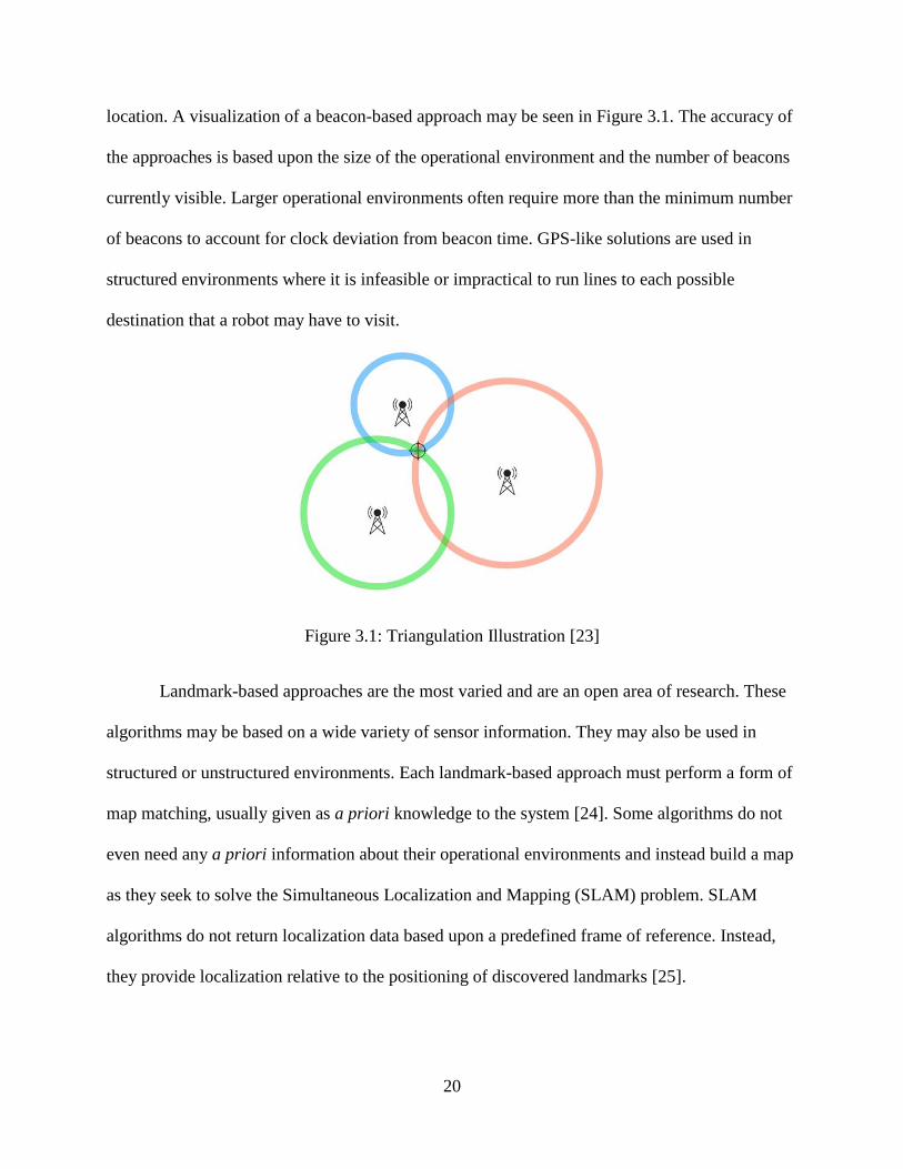
location. A visualization of a beacon-based approach may be seen in Figure 3.1. The accuracy of

the approaches is based upon the size of the operational environment and the number of beacons

currently visible. Larger operational environments often require more than the minimum number

of beacons to account for clock deviation from beacon time. GPS-like solutions are used in

structured environments where it is infeasible or impractical to run lines to each possible

destination that a robot may have to visit.

Figure 3.1: Triangulation Illustration [23]

Landmark-based approaches are the most varied and are an open area of research. These

algorithms may be based on a wide variety of sensor information. They may also be used in

structured or unstructured environments. Each landmark-based approach must perform a form of

map matching, usually given as a priori knowledge to the system [24]. Some algorithms do not

even need any a priori information about their operational environments and instead build a map

as they seek to solve the Simultaneous Localization and Mapping (SLAM) problem. SLAM

algorithms do not return localization data based upon a predefined frame of reference. Instead,

they provide localization relative to the positioning of discovered landmarks [25].

21

Landmarks are uniquely identifiable objects that serve a similar role to the beacons found

in GPS-like applications. The difference is that the landmarks can be naturally occurring or

artificial. Landmark-based approaches can use any uniquely identifiable object as a landmark

and are relatively unhindered by landmark placement and the size of the operational

environment. Landmark-based solutions are more computationally expensive than other methods

of localization. Their versatility makes them a necessity for any robotics platform operating in an

unstructured environment [26].

3.2 Case Study

The autonomous rover built for the RMC was tasked to operate in a semi-structured

environment. The environment was of known size and had global landmarks, walls, available for

use in localization. The environment was only semi-structured due to the unknown placement of

obstacles in the obstacle zone. The only modification allowed to the operational environment at

the RMC was the placement of a beacon on the collection bin. This restriction makes line

following a nonviable option. Ideally the beacons used in a GPS-like algorithm would be spaced

throughout the operational environment. With the RMC rules, all beacons would be located

within 1.6 m of each other creating an implementation that would be far from ideal. Dead

reckoning does not retain the accuracy needed for the task over the operational period due to

compounding error. Thus, a landmark-based approach is used.

The landmarks used are the walls of the operational environment. Since the size of the

operational environment is given within the specifications, a global map is created using this a

priori knowledge. A single 2D LIDAR scan is taken at a height so as to only detect the

landmarks used for localization. The lines which define the landmarks are extracted. In [26] and

[27] a 2D LIDAR scan is used to build a map and determine the location of a rover with respect

22

to the landmarks generated by walls of a room. This is performed using an angle histogram. The

algorithm presented in the case study takes advantage of the organization of the data coming

from the LIDAR, and removes the angle histogram. Since the data is ordered contiguously, it is

possible to treat the data as a single line. If a point deviates too far from the line, the data is

separated at that point and the process run recursively until each segment contains only those

points which represent a wall. The intersections of the walls are extrapolated and all possible

transforms for the data are calculated. Due to the symmetry of the operational environment and

the landmarks therein, this approach generates several possible transforms. This symmetry is

broken and the correct transform identified using two different methods. If the localization in

question is the initial localization, the symmetry of the operational environment is broken via the

a priori knowledge that the starting location must be within one portion of the environment. If

the localization is not the initial localization, the symmetry is broken through the yaw provided

by the AHRS. The possible transform with the yaw closest to that given by the AHRS is the

correct transform. This method allows for a substantial error in the yaw when selecting the

transform due to the symmetry of the operational environment only occurring in 45° increments.

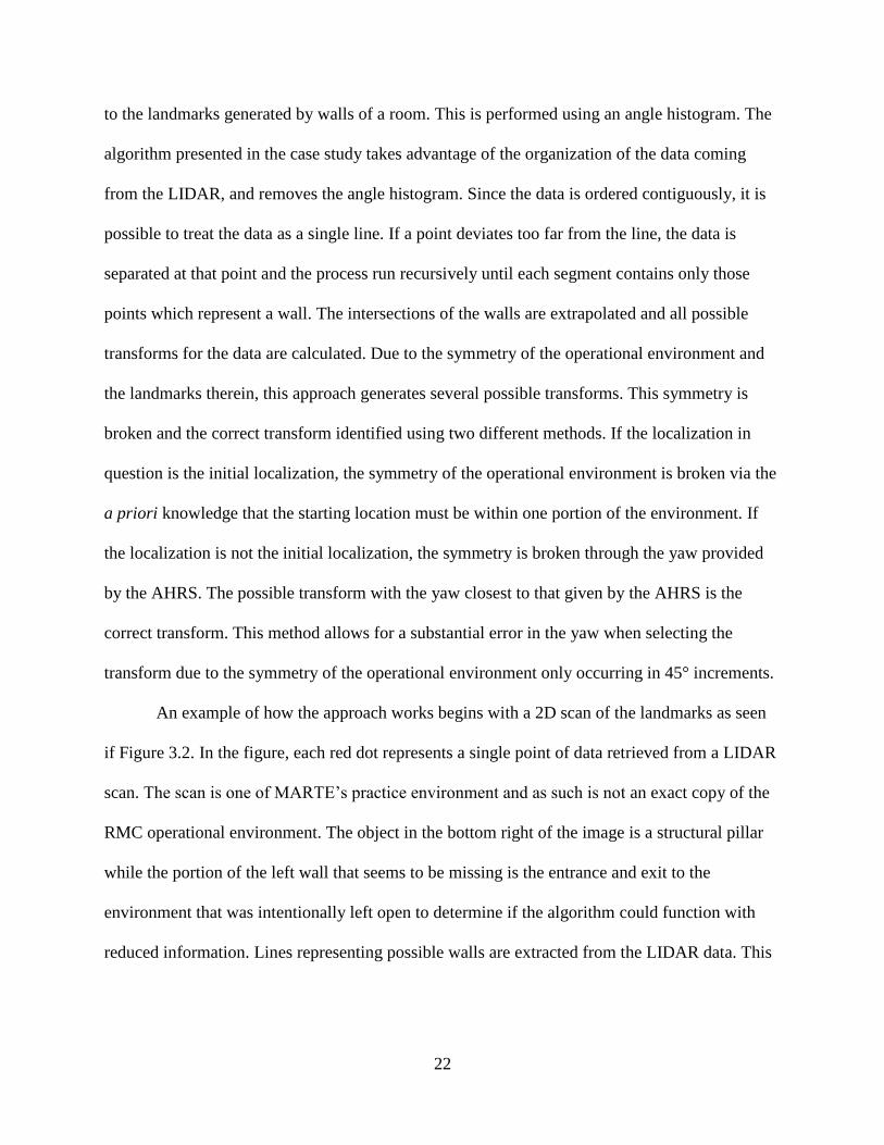
An example of how the approach works begins with a 2D scan of the landmarks as seen

if Figure 3.2. In the figure, each red dot represents a single point of data retrieved from a LIDAR

scan. The scan is one of MARTE’s practice environment and as such is not an exact copy of the

RMC operational environment. The object in the bottom right of the image is a structural pillar

while the portion of the left wall that seems to be missing is the entrance and exit to the

environment that was intentionally left open to determine if the algorithm could function with

reduced information. Lines representing possible walls are extracted from the LIDAR data. This

23

operation takes advantage of the ordering of the data as it is presented. The data returned from

the LIDAR is a continuous stream from left to right.

Figure 3.2: 2D Scan of Environment Landmarks

Each data point is ordered by its angle. The lines are extracted by attempting to draw a line

between the first and last data point of the set. If a single data point of the set has a perpendicular

distance to the line that is greater than an acceptable threshold, the data set is split into two

subsets. The subsets consist of the points before the pivot and those after the pivot. The pivot is

included in each of the subsets. The algorithm is then run recursively upon the two new data sets.

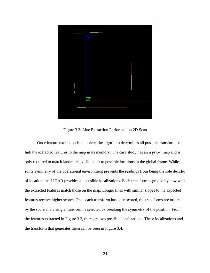
Once a line is found that matches a subset of data, it is recorded as a possible landmark as long

as it has a statistically significant number of data points. The possible landmarks generated from

the scan shown in Figure 3.2 can be seen in Figure 3.3.

24

Figure 3.3: Line Extraction Performed on 2D Scan

Once feature extraction is complete, the algorithm determines all possible transforms to

link the extracted features to the map in its memory. The case study has an a priori map and is

only required to match landmarks visible to it to possible locations in the global frame. While

some symmetry of the operational environment prevents the readings from being the sole decider

of location, the LIDAR provides all possible localizations. Each transform is graded by how well

the extracted features match those on the map. Longer lines with similar slopes to the expected

features receive higher scores. Once each transform has been scored, the transforms are ordered

by the score and a single transform is selected by breaking the symmetry of the position. From

the features extracted in Figure 3.3, there are two possible localizations. These localizations and

the transform that generates them can be seen in Figure 3.4.

25

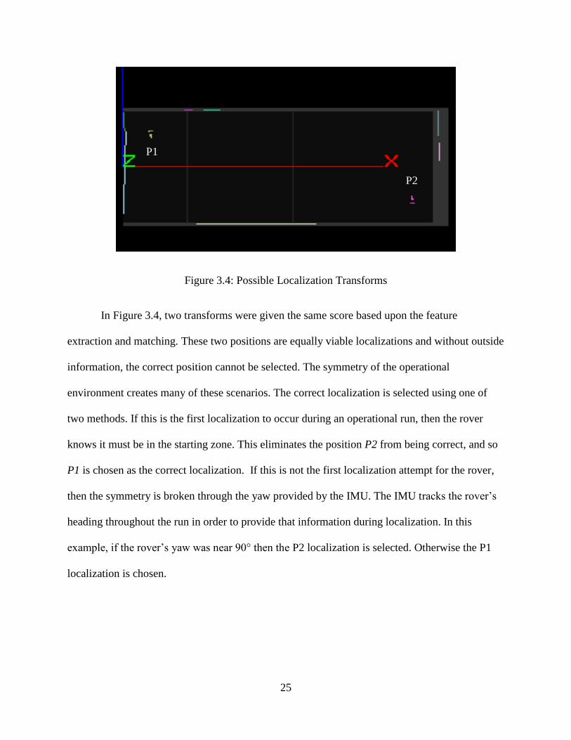
Figure 3.4: Possible Localization Transforms

In Figure 3.4, two transforms were given the same score based upon the feature

extraction and matching. These two positions are equally viable localizations and without outside

information, the correct position cannot be selected. The symmetry of the operational

environment creates many of these scenarios. The correct localization is selected using one of

two methods. If this is the first localization to occur during an operational run, then the rover

knows it must be in the starting zone. This eliminates the position P2 from being correct, and so

P1 is chosen as the correct localization. If this is not the first localization attempt for the rover,

then the symmetry is broken through the yaw provided by the IMU. The IMU tracks the rover’s

heading throughout the run in order to provide that information during localization. In this

example, if the rover’s yaw was near 90° then the P2 localization is selected. Otherwise the P1

localization is chosen.

P1

P2

26

3.3 Testing

The localization approach developed for MARTE was tested in a simulated competition

environment on the campus of The University of Alabama. The rover was placed in twenty

different position and orientation combinations throughout the environment. Each position was

tested with five separate LIDAR scans for repeatability. The location of the rover was measured

manually and the results were compared. Tests were considered successful if the localization was

within 75 mm of the measured value. This standard is based on the resolution of the occupancy

grid that is created by the obstacle detection algorithm described in Chapter 4. The results of

testing can be seen in Figure 3.5. Fifty percent of tests resulted in localizations that were within

25 mm of the measured value. Another 35% of localizations were within 50 mm. The

localization algorithm meets the aforementioned standard in 95% of test cases.

Figure 3.5: Average Error for Localization Testing

50%35%

10%

5%Avg Error of Tests at a Location

< 25 mm

25 - 50 mm

50 - 75 mm

75 - 100 mm

27

There are several possible explanations for the remaining 5% of cases that do not meet

the 75 mm requirement. The algorithm output is compared against manual measurements which

are subject to measurement error. All tests that failed to meet the standard were taken in a single

location. However, further testing at that specific location did not reveal the same failure of

localization.

28

CHAPTER 4

OBSTACLE DETECTION

4.1 Obstacle Detection Algorithms

Obstacle detection is an area of ongoing research in autonomous robotics. The sensors

used in obstacle detection are dependent upon the intended operational environment of the rover.

A non-exhaustive list of possible sensors include: infrared, vision, laser, and ultrasonic detection

[28]. Regardless of the sensor used to detect obstacles, algorithms for obstacle detection can be

broken into two categories. Reactive algorithms, often classified as obstacle avoidance, are

tightly integrated with the autonomous controller. These algorithms detect obstacles after the

rover has already set out on a course and are used to detect obstacles within the path in real-time.

The autonomous controller is interrupted and evasive action is taken if it is deemed necessary. In

contrast to reactive algorithms, proactive algorithms attempt to detect obstacles before operation

has begun. These algorithms provide input into path planning methods that precompute the

rover’s path to avoid obstacles before movement continues.

Reactive algorithms can be implemented with 1D, 2D, or 3D sensors. The most common

of these include IR, ultrasonic, and vision. As previously mentioned, reactive algorithms are

tightly coupled with the autonomous controller, including interrupting the controller during

normal operation. Since these methods occur during the traversal of an already determined path,

they are not used in path planning, but rather path alteration. Reactive obstacle detection is

generally paired with an appropriate avoidance algorithm. An example would be the pairing of

29

IR obstacle detection with a Bug algorithm [29]. Reactive algorithms can be paired with

proactive algorithms in order to provide any necessary alterations to an already planned path.

Proactive obstacle detection is generally implemented with 3D data, often a stereo

camera or LIDAR. Proactive algorithms are distinct from the autonomous controller and are

consulted before the rover sets off for the traversal of a path. Proactive obstacle detection is

paired with path planning algorithms to fulfill the sense, plan, and act paradigm of robotics. In

this paradigm, the operational environment is sensed before any actions are taken. The data is

processed and an operational plan is constructed which allows for the completion of the

autonomous system’s goals with the least exposure to danger. After the plan has been

determined, the autonomous controller acts based on the knowledge previously attained to fulfill

the operational plan.

4.2 Case Study

A proactive approach is used to provide obstacle detection on the case study rover. Many

IR sensors experience error in the direct sunlight to which the rover is exposed. The obstacles

and terrain are of the same material and dust is suspended during operation. For these reasons, a

vision-based detection system is considered difficult to implement. The approach that is used is

based upon the actuation of a 2D LIDAR. Scans are taken at regular angular intervals and unified

into a single 3D pointcloud. The pointcloud is downsampled, divided into 1 m2 sections. The

ground planes of each section are generated and removed. The remaining points left in the

pointcloud represent possible obstacles. The points are grouped using Euclidean Clustering and

if a cluster contains a number of points greater than a set threshold, it is marked as an obstacle.

Two types of obstacles are identified by the algorithm. Convex obstacles are those that extend

30

above ground such as rocks. In contrast, concave obstacles are ones that form from the removal

of portions of the ground plane. Craters are one example of concave obstacles.

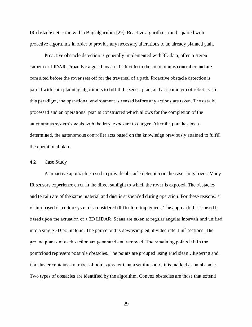
A possible obstacle zone configuration is shown in Figure 4.1. Placed within the zone are

three convex obstacles and two concave obstacles. The LIDAR is actuated by the active

stabilization system to form a 3D pointcloud image of the obstacle zone. The pointcloud

corresponding to Figure 4.1 may be seen in Figure 4.2. Each dot represents one point of data

returned from the LIDAR. The obstacles are highlighted in Figure 4.2. The convex obstacles are

within the red boxes with annotations: R1, R2, and R3. The concave obstacles can be found

within the blue boxes with annotations: C1 and C2. This scheme will be consistent throughout

this example.

Figure 4.1: Example Obstacle Zone

R1

R2

R3

C1

C2 N

31

Figure 4.2 Pointcloud of Obstacle Zone with Obstacles Highlighted

Once the pointcloud has been gathered, it is downsampled. In this case it is downsampled

so that there is no more than one point of data within 50 mm3. Places where multiple points fall

within the same cubic region are averaged and a new data point that represents the region as a

whole is used. The reduction serves multiple purposes. It reduces the size of the data set. This

allows for faster execution. Downsampling also reduces the impact of nonuniform data much

like an averaging filter on an image. Lastly, due to the way in which the data is collected, a

greater percentage of the data points are closer to the sensor. Downsampling helps alleviate the

biased distribution of data points to a manageable level.

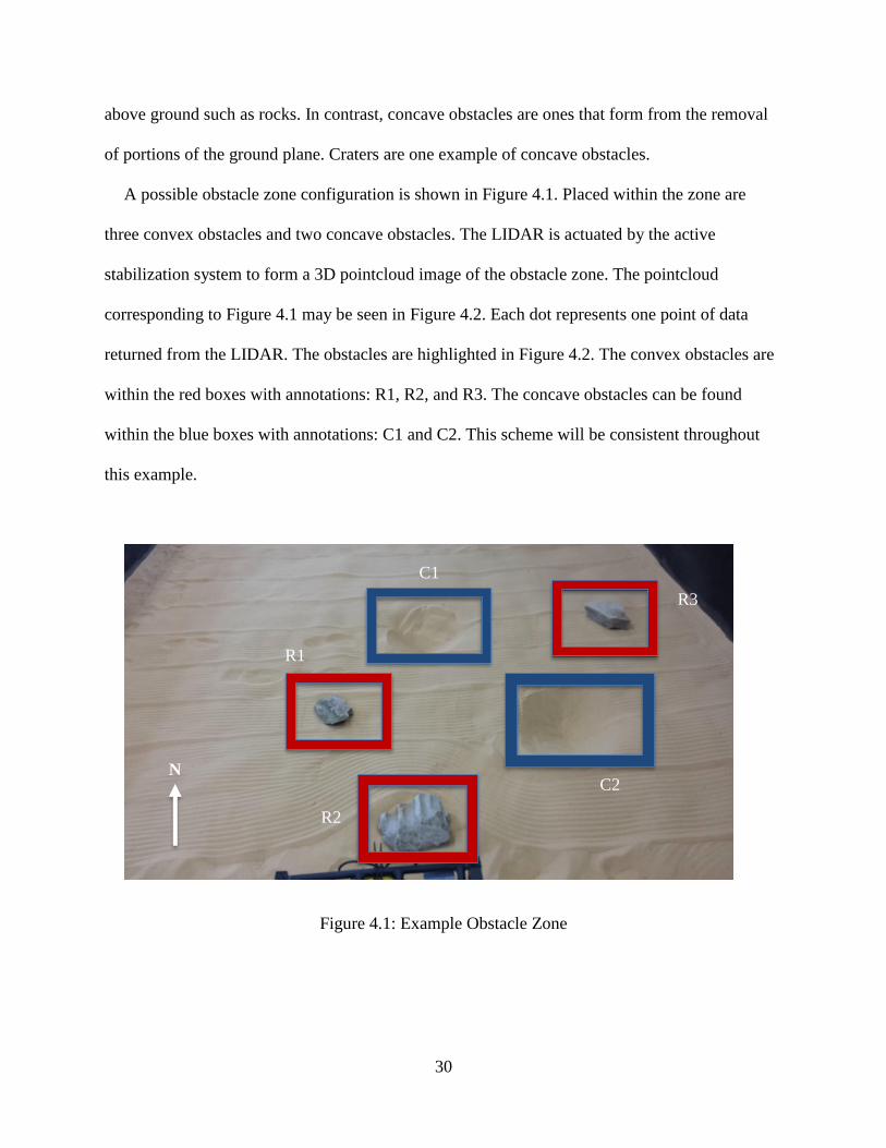
After the pointcloud has been downsampled, it is divided into overlapping pointclouds of

1 m3 as can be seen in Figure 4.3. The Random Consensus Method (RANSAC) [30] is run on

each individual pointcloud to determine the best plane of fit for its data. The best plane of fit is

the ground plane of the smaller pointcloud. RANSAC works by selecting a subset of the

pointcloud and defining them as inliers. It fits a plane to those inliers and checks every data point

against the created plane. The plane is scored based on its fit to the data points in the pointcloud.

R1

C1

R2 C2

R3

N

32

This process is repeated until either a plane receives an adequately high score or a certain

number of iterations have been attempted. Once a ground plane is determined, the data points

that constitute the ground plane are removed from the pointcloud. The points left in the point

cloud after the plane extraction represent possible obstacles.

Figure 4.3: Data is Divided into Smaller Local Pointclouds

Once each ground plane is removed, the remaining data points are reconstituted to form a

single pointcloud that holds all possible obstacle data points. Some of these points may be dust

or erroneous measurements due to environmental conditions. It is unlikely that several of these

data points would be congregated together. Euclidean Clustering [31] is used to determine

whether a possible obstacle data point is erroneous or correct. Euclidean Clustering is often used

to identify spatially similar data points. Each data point is clustered with any data points within a

Euclidean distance of 100 mm. This process is repeated on every point that enters the cluster

until no new points can be added. The new cluster is evaluated and if it contains enough

members it is considered an obstacle, otherwise it is discounted. Regardless of whether it is

R1

R2

C1

C2

R3

N

33

defined as an obstacle, the points that constitute the cluster are removed from the overall

pointcloud and the process is repeated until the pointcloud is empty.

The path planning algorithm discussed in the next chapter requires an occupancy grid on

which to operate. The clusters determined to be obstacles using Euclidean Clustering are

evaluated to determine whether they are concave or convex obstacles. This is determined by

comparing the data points with the local ground plane determined by RANSAC. Once the

obstacle has been categorized, its members are iterated through and translated into grid spaces on

the occupancy grid. The grid spaces used by the autonomous rover measure 50 mm x 50 mm.

The confines of the operational environment are predefined in the occupancy grid as convex

obstacles. The occupancy grid derived from the obstacle zone found in Figure 4.1 can be seen in

Figure 4.4. A similar visualization scheme is used wherein convex obstacles are shown in red

while concave obstacles are blue. One note to make is the inclusion of a fourth convex obstacle,

R4. The appearance of this obstacle is due to the division of ground planes occurring in the

middle of a concave obstacle. If this occurs it can result in the far rim of the obstacle to be

classified as a convex obstacle.

The algorithms that comprise MARTE’s obstacle detection algorithm are not unique. In

[32] a LIDAR was used to create a 3D pointcloud which was used for obstacle detection.

RANSAC is a common algorithm for the determination of plane generation based upon sampled

data [30]. Euclidean Clustering is often used to identify spatially similar data points [31]. While

case study implementations of these algorithms are not unique, MARTE combines them to form

an obstacle detection algorithm to be executed on embedded hardware. The implementation is

based upon the Pointcloud Library (PCL) [31].

34

Figure 4.4: Occupancy Grid of Example Obstacle Zone

4.3 Testing

The obstacle detection algorithm was tested by placing convex and concave obstacles at

0.5 m, 1.5 m, and 2.5 m from the lidar. The concave obstacles were craters measuring

approximately 475 mm in diameter and 150 mm deep. The convex obstacles were rocks of

varying sizes. The sizes of rocks used in ascending order are 85 mm, 115 mm, and 150 mm in

height. The results of the tests can be seen in Figure 4.5. At 0.5 m, the algorithm has no trouble

in detecting either type of obstacle. Once the obstacles are moved to 1.5 m, the 85 mm rock is

lost in 50% cases. These cases may occur since the threshold for an obstacle in the test is 75 mm.

One reason for the variability is the fact that RANSAC randomly chooses points for the ground

plane and as such the same ground plane will not necessarily be chosen even on the same data set

if run multiple times. In addition, since the height of the small obstacle is close to that of the

threshold, it is possible that ripples in the terrain and natural undulations may bring it closer to

that threshold when compared against a local ground plane.

R2

R1

R3

R4

C2

C1

N

35

The detection rate of the concave obstacles also suffers at greater distances. This is due to

the height of the LIDAR which is set at 0.35 m in these tests. Concave obstacles, by their very

definition, do not extend above the ground plane, but are recesses into it. Thus, to record data

points in the interior of the obstacle, the sensor must be able to see down into it. To achieve this,

the sensor should be placed as high as possible for optimal performance. However, the LIDAR

being used to perform obstacle detection is also multiplexed to perform localization, and the

compromise in position led to a decrease in the detection rate of concave obstacles. This is

deemed an acceptable compromise in the rover’s operational principles. The trend continues at

2.5 meters where the ability to detect both the small rock and the craters has been eliminated due

to the conditions mentioned above. The algorithm has no trouble detecting the medium and large

sized rocks at this distance; however there is a point where this ability will also diminish due to

the resolution of the sensor stabilization system.

Figure 4.5: Obstacle Detection Testing Results

0

20

40

60

80

100

0.5 1.5 2.5

Pe

rce

nta

ge o

f O

bst

acle

s Fo

un

d (

%)

Distance (m)

85 mm Convex

115 mm Convex

150 mm Convex

150 mm Concave

36

CHAPTER 5

PATH PLANNING

5.1 Path Planning Algorithms

Path planning is the formation of a collection of waypoints designed to guide a rover

from its current position to a goal state while exposing the rover to minimal danger. Path

planners are used in the Hierarchical Paradigm of the sense, plan, and act primitives of robot

operation [33]. The planning algorithms can be divided into two subtypes: motion planning and

discrete planning. Motion planning algorithms are based on mathematically modeling the rover

and its environment. These algorithms tend to be more accurate than their discrete counterparts,

however they involve a computational complexity that increases execution time. In contrast,

discrete planning algorithms operate on a graph or grid space. These algorithms tend to provide

less accurate results but are computationally simple.

Motion planning algorithms use a geometric representation of the rover and its

environment to determine the possible locations for rover placement. To help with this task, a

configuration space is used. This space describes all possible transforms that can be applied to

the robot during path execution. The topological space is often used as the configuration space.

Motion planners use algebraic representations of rover kinematics to plan the motion of the rover

during the path. This allows for accurate generation of maneuvers that are within the rover’s

capabilities. Motion planning algorithms can also be subdivided into two categories. Sampling-

based algorithms such as Probablistic Roadmaps take samples from across the possible paths for

37

the rover [34]. Much like the RANSAC algorithm used in the obstacle detection implementation

in the case study, sampling-based motion planners are not guaranteed to find the optimal

solution. Combinatorial motion planners such as Canny’s algorithm find optimal solutions to

path planning problems, but can have greater execution times than sampling-based motion

planners [35].

Discrete path planners are grid or tree-based in their implementations. Due to the

discretization of the rover, its environment, and the operation kinematics of the rover, discrete

path planners are suboptimal. In addition, they are subject to inherent error for the same reasons.

Discrete path planners are easy to implement and have the fastest execution time of all path

planners. Discrete path planners can be subdivided into two categories: unguided and guided

planners. Unguided planners such as Djikstra’s Algorithm, must perform an exhaustive search of

the problem space to guarantee an optimal solution [36]. The performance of unguided discrete

planners suffers significant degradation as the size of an operational environment becomes too

large or the required resolution of the problem space is too small. Guided discrete planners do

not need to evaluate the entire problem space to find an optimal solution. Guided planners, such

as A*, make use of a heuristic to determine the order in which they evaluate each node in the

graph [37]. These planners offer significant performance improvements over unguided searches

since they do not need to evaluate the entire problem space.

5.2 Case Study

A* has been used numerous times as the core path planning algorithm in robotics [38]. In

addition, Bresenham’s algorithm has also been used to alleviate certain cases caused by grid-

based pathing algorithms [39]. The case study implementation is a modified A* guided search

algorithm that is applied over an occupancy matrix problem space. The modifications allow

38

obstacle expansion to account for rover dimensions and the kinematics are simplified to zero

point turns and straight lines. Post-processing is performed on the A* results to reduce the path

to minimal waypoints. Bresenham’s algorithm is then used to check for unnecessary waypoints

due to grid angle limitations [39].

A* is an optimized form of Dijkstra’s Algorithm. Dijkstra’s Algorithm is transformed

into a heuristic driven guided search. A* is a best first search that is widely used in robotic path

planning implementations. The resulting algorithm is considered admissible, meaning it finds the

optimal solution to the problem, so long as the heuristic that is used to calculate the distance

between the current node and the goal node does not overestimate the distance between the two

nodes. The heuristic used in the case study is Chebyshev Distance. Chebyshev Distance is a

heuristic that is similar to Manhattan Distance on a grid [40]. Where Manhattan Distance does

not allow the search to travel in diagonals, Chebyshev Distance does. Chebyshev Distance has

been proven to be admissible and thus the entire A* algorithm is admissible, guaranteeing an

optimal solution to a presented data set.

During the search, A* defines two types of nodes. The nodes in the open set have yet to

be evaluated. The nodes in the closed set have already been evaluated. Initially, the closed set is

empty, and the open set contains the start node. The algorithm selects the node from the open set

that has the lowest distance to the goal node. Once the node has been selected, the distance from

the start node is determined. This distance does not need to be the same as that which computes

the search heuristic. Changes made to the scoring system do not affect the admissibility of the

algorithm, but rather change the operating parameters of what defines an optimal path. Once a

node has been scored, if it is not the goal node then each of its eight possible neighbors are added

to the open set so long as the expanded occupancy matrix does not have a neighbor marked as an

39

obstacle. Once this is completed, the current node is placed in the closed set so as to not be

evaluated again. The process then repeats with the algorithm selecting the node from the open set

with the shortest distance to the goal, until the goal is reached.

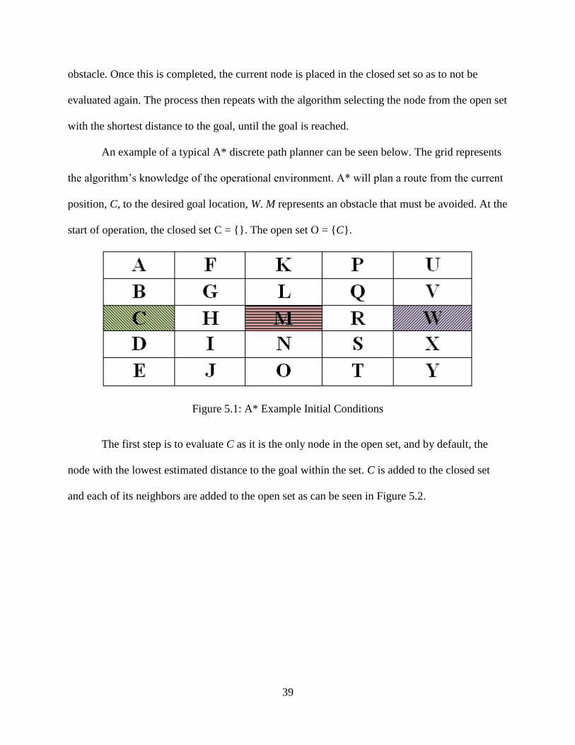
An example of a typical A* discrete path planner can be seen below. The grid represents

the algorithm’s knowledge of the operational environment. A* will plan a route from the current

position, C, to the desired goal location, W. M represents an obstacle that must be avoided. At the

start of operation, the closed set C = {}. The open set O = {C}.

Figure 5.1: A* Example Initial Conditions

The first step is to evaluate C as it is the only node in the open set, and by default, the

node with the lowest estimated distance to the goal within the set. C is added to the closed set

and each of its neighbors are added to the open set as can be seen in Figure 5.2.

40

Figure 5.2: Results of Iteration 1

At the end of the first iteration C = {C} and O = {B, D, G, H, I}. The second iteration

evaluates the nodes in the open set and finds that H is the closest to the goal. It is added to the

closed set and each of its neighbors is added to the open set. The exception is M which is

identified as an obstacle. As such, it will not be added to the open set. This is the manner in

which A* deals with obstacles or path obstructions. The result of the second iteration is a C =

{C, H} and an O = {B, D, G, I, L, N}. The results of the second iteration can be seen in Figure

5.3.

Figure 5.3: Results of Iteration 2

41

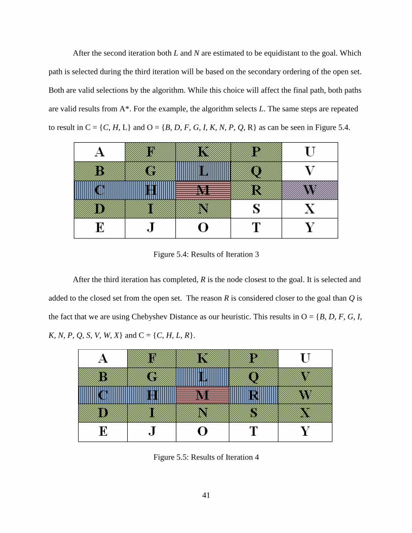
After the second iteration both L and N are estimated to be equidistant to the goal. Which

path is selected during the third iteration will be based on the secondary ordering of the open set.

Both are valid selections by the algorithm. While this choice will affect the final path, both paths

are valid results from A*. For the example, the algorithm selects L. The same steps are repeated

to result in C = {C, H, L} and O = {B, D, F, G, I, K, N, P, Q, R} as can be seen in Figure 5.4.

Figure 5.4: Results of Iteration 3

After the third iteration has completed, R is the node closest to the goal. It is selected and

added to the closed set from the open set. The reason R is considered closer to the goal than Q is

the fact that we are using Chebyshev Distance as our heuristic. This results in O = {B, D, F, G, I,

K, N, P, Q, S, V, W, X} and C = {C, H, L, R}.

Figure 5.5: Results of Iteration 4

42

At the end of the fourth iteration, the goal node (W), is added to the open set. Once this

occurs, it is guaranteed to be added to the closed set during the fifth iteration due to it being the

only node with a distance to goal of 0. The algorithm completes with C= {C, H, L, R, W} and O

= {B, D, F, G, I, K, N, P, Q, S, V, X} after the fifth iteration. The ending values of the open and

closed sets can be visualized in Figure 5.6. The closed set may contain nodes that do not belong

to the final path. This occurs when the algorithm follows a false trail before finding the correct

path. The nodes of the closed set include pointers to the parent nodes to allow for path

reconstruction since the closed set may contain misleading nodes.

Figure 5.6: Results of Iteration 5

Modifications were made to the standard A* algorithm to optimize it for the case study.

Graph algorithms treat the robot as if it is an infinitesimally small point. This is obviously not

true in real life. To accommodate for this assumption, the obstacles in the occupancy grid must

be expanded. This process involves marking every grid space within half the robot diameter as

an obstacle of the same type. This process works well for robots that have a length roughly equal

to their width. This is not true in the case study. MARTE’s wheelbase is significantly longer than

its axle track. A natural response to this would be to expand the obstacles in the grid by half the

longest dimension of the vehicle. This approach suffers as the difference in physical dimensions

43

increases. In the case study, this approach led to the elimination of many viable paths due to the

fact that the robot could not perform a zero point turn. To combat this, the A* algorithm is

modified to have two different obstacle expansion grids. The first grid is the expansion by half

the width of the vehicle. This grid is known as the Forward Grid. The second grid is the

expansion of the obstacles by half of the largest dimension of width and length. This grid

represents the places in which the robot can safely perform a zero point turn. This grid is known

as the Turn Grid. The algorithm is modified to not only look at the position of the grid space it is

evaluating, but also the direction of travel into that space. This causes a growth of the problem

space by a factor of eight, the number of ways to enter a grid space. The growth in problem

space is acceptable to attain proper planning and the detection of paths that are otherwise

unavailable to the algorithm.

The second major modification to A* was in the definition of the optimal path. The

scoring of each node, as it is placed into the closed set, is generally defined using the same

heuristic as is used in the node selection from the open set. This score is often the distance

between the node being placed into the closed set and the start node of the algorithm. This results

in the detection of the shortest possible path from the starting location to the goal. The shortest

path is not necessarily the best in every application. The shortest path often skirts the edges of

obstacles and often involves a large number of turns in a complicated environment. These

characteristics complicate the function of rover control and provide little room for error on the

parts of the obstacle detection, localization, and autonomous controller. To combat this, the

optimal path during the case study was defined as the path that consisted of the fewest turns

resulting in preferences towards long straight path segments. To achieve this goal, the score of

each node is equal to the distance traveled from the starting location, so long as the rover does

44

not have to change orientations between the last node and the current node. If the rover must

change direction to reach the node currently being evaluated, then the score of that node is

penalized heavily. This penalization of change of direction results in the desired path

prioritization while allowing for the generation of complex paths that may be needed in

complicated terrain.

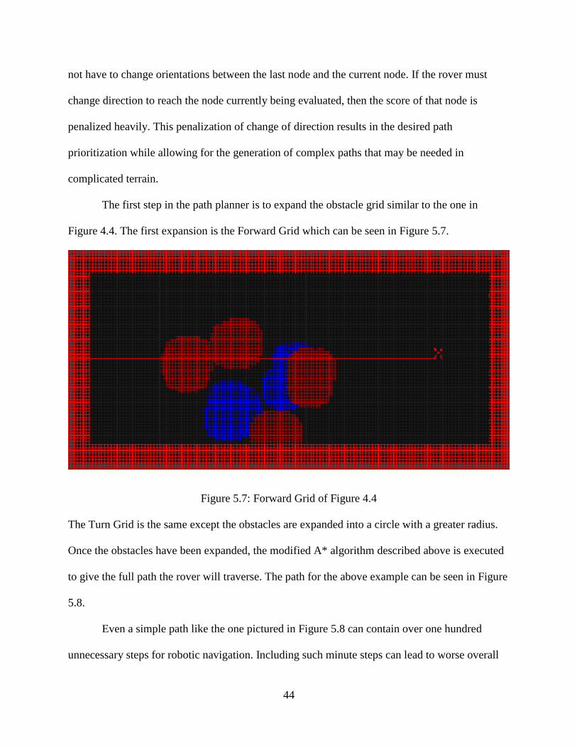
The first step in the path planner is to expand the obstacle grid similar to the one in

Figure 4.4. The first expansion is the Forward Grid which can be seen in Figure 5.7.

Figure 5.7: Forward Grid of Figure 4.4

The Turn Grid is the same except the obstacles are expanded into a circle with a greater radius.

Once the obstacles have been expanded, the modified A* algorithm described above is executed

to give the full path the rover will traverse. The path for the above example can be seen in Figure

5.8.

Even a simple path like the one pictured in Figure 5.8 can contain over one hundred

unnecessary steps for robotic navigation. Including such minute steps can lead to worse overall

45

performance of the system. To avoid this, post processing is performed on the path to eliminate

all nodes except where the rover should change direction. These critical points are known as

waypoints. The post processing of Figure 5.8 can be seen in Figure 5.9.

Figure 5.8: Full Path Returned by Modified A*

46

Figure 5.9: Post-processing Produced Path

After the waypoint reduction, a form of Bresenham’s Line Algorithm is performed to see

if any path exists between two unconnected waypoints. Bresenham’s Line Algorithm was

developed to draw straight lines on computer imaging screens, which are represented as grids.

The algorithm allows for the elimination of waypoints caused by the angle limitations imposed

by the use of grids. Since grid calculations only allow angles in 45° increments, Bresenham’s

Line Algorithm was developed to approximate lines with other angles on computer screens. The

same approach can be taken to determine straight lines through an occupancy matrix.

Bresenham’s algorithm is useful for eliminating step patterns that can occur due to the

restrictions on grid calculations. The elimination of this step pattern removes unnecessary

waypoints from the path. These unnecessary waypoints cost operation time since MARTE

performs overhead operations at each waypoint.

47

CHAPTER 6

SYSTEM TESTING

The rover constructed during the case study was entered into the 2014 NASA Robotic

Mining Competition. The results of each run in the competition environment can be seen in

Table 6.1. The first run resulted in a loss of localization due to accumulated error in the AHRS

and the relative vertical positioning of the LIDAR with relation to the landmarks. To correct

these problems, the LIDAR mount was physically lowered and additional recalibration points

were added to the rover’s operational procedure. The second run was a fully teleoperated run to

allow for updates to the autonomous system and to give the pilots practice time in the

competition environment. Runs 3, 5, and 6 were all completed successfully using fully

autonomous operation for the duration of the run. Run 4 experienced a hardware mounting error

when the mounting of the IMU shifted during operation, leading to invalid sensor stabilization.

MARTE was the only rover to actively detect and avoid obstacles. MARTE was awarded first

place from NASA at the competition.

48

Run Date Qualified? Operational Mode Notes

1 May 19,

2014

Yes Autonomous /

Teleoperation

Lidar mounting error;

AHRS compound error;

Fixed before Run 3

2 May 20,

2014

Yes Teleoperation

3 May 20,

2014

Yes Autonomous

4 May 21,

2014

Yes Autonomous /

Teleoperation

IMU mount shifted causing sensor

stabilization error

5 May 23,

2014

Yes Autonomous

6 May 23,

2014

Yes Autonomous

Table 6.1: RMC Run Results

The execution times of the component algorithms of MARTE’s autonomous software can

be found in Table 6.2. Execution time of the pathfinding algorithm in a best case scenario, when

a clear path exists between the current and goal locations, is ~475 ms. The execution time in

worst case scenarios is ~1,600 ms. A worst case scenario would consist of a complicated

obstacle structure that would lead to a goal that is completely surrounded by obstacles. This

would require A* to be executed three times with differing levels of obstacle traversal allowed.

Gimbal leveling time is a composite. The first portion is the execution time measured from the

acquisition of new data from the IMU until the update of the DCM. The second portion is the

execution time of the algorithm that updates the gimbal servos based upon MARTE’s

orientation. The composite of these times is less than 1 ms. The localization and gimbal leveling

algorithms can be run in real-time applications as presented. The Path Planning algorithm could

not be run in a real-time application due to its extended execution time. It could be run, as it was

with MARTE, as a planning or staging component of a real-time application. Obstacle detection

could be run in a real-time application so long as the algorithm could receive data to make

decisions for the next 200 ms of operation.

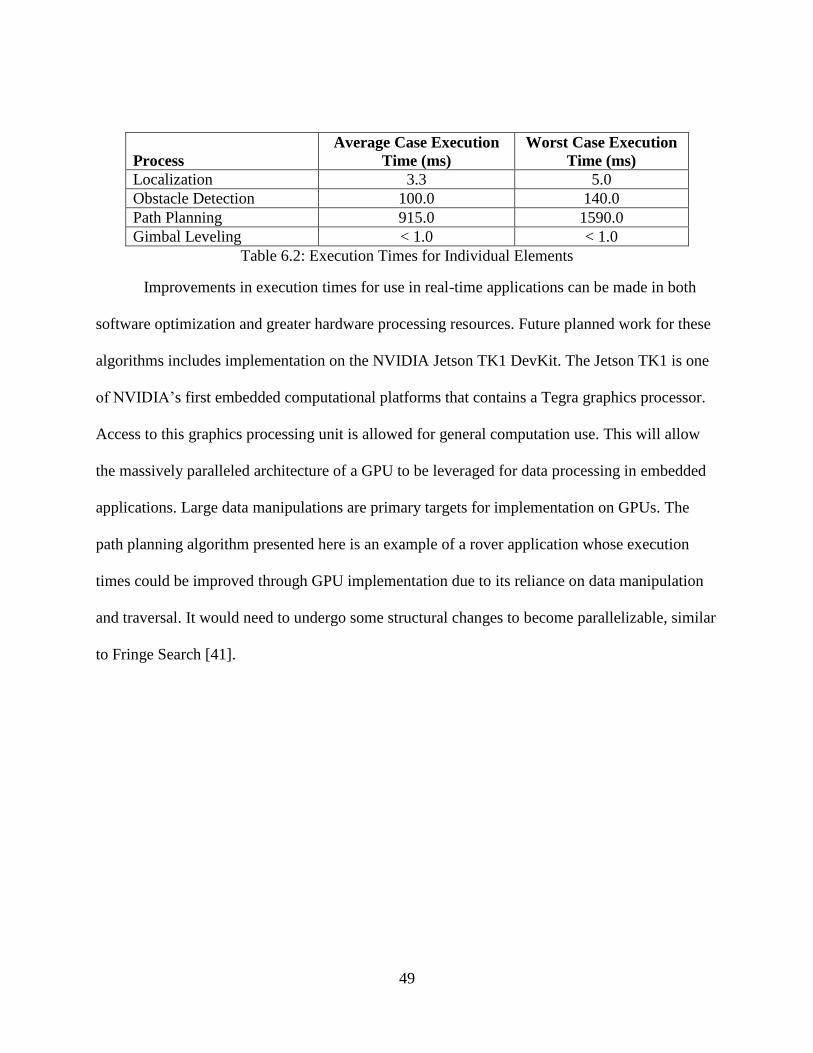
49

Process

Average Case Execution

Time (ms)

Worst Case Execution

Time (ms)

Localization 3.3 5.0

Obstacle Detection 100.0 140.0

Path Planning 915.0 1590.0

Gimbal Leveling < 1.0 < 1.0

Table 6.2: Execution Times for Individual Elements

Improvements in execution times for use in real-time applications can be made in both

software optimization and greater hardware processing resources. Future planned work for these

algorithms includes implementation on the NVIDIA Jetson TK1 DevKit. The Jetson TK1 is one

of NVIDIA’s first embedded computational platforms that contains a Tegra graphics processor.

Access to this graphics processing unit is allowed for general computation use. This will allow

the massively paralleled architecture of a GPU to be leveraged for data processing in embedded

applications. Large data manipulations are primary targets for implementation on GPUs. The

path planning algorithm presented here is an example of a rover application whose execution

times could be improved through GPU implementation due to its reliance on data manipulation

and traversal. It would need to undergo some structural changes to become parallelizable, similar

to Fringe Search [41].

50

CHAPTER 7

CONCLUSIONS AND FUTURE WORK

This paper has presented the basis for autonomous rover navigation in the form of sensor

stabilization, localization, obstacle detection, and path planning. These issues were also

addressed through the use of a case study involving an excavation rover that was entered into the

2014 NASA Robot Mining Competition. An active sensor stabilization system was developed to

stabilize a LIDAR. This LIDAR was time multiplexed to perform 2D scans used in localization

and 3D scans for obstacle detection. Localization was accomplished through a landmark-based

approach in a semi-structured environment. Obstacle detection used 3D pointclouds generated by

the LIDAR and performed RANSAC and Euclidean Clustering to generate an occupancy grid.

This occupancy grid was expanded and used as the problem space for a modified A* path

planning algorithm. All processing pertaining to the autonomous system was performed onboard

and in near-real time. The rover entry discussed in this paper was awarded first place by NASA

and industry judges.

Improvements can be made to the approaches taken in each area. The sensor stabilization

system can be improved in several areas. Stepper motors can be used to replace the servo motors

for greater resolution and feedback. In addition, the IMU could be upgraded to one with less

drift. A higher degree estimation of integration may also improve performance by reducing the

error inherent in the calculation. Finally, a Kalman Filter could be implemented with multiple

IMUs oriented along differing axes. Localization can be upgraded to a generalized approach that

51

would perform in situations outside of the given operational environment. Obstacle detection can

improve the detection rate of concave and small convex obstacles through the implementation of

a mesh or gradient-based algorithm. Path planning could be upgraded to an incremental heuristic

search approach which would allow the same system to perform as both a reactive and proactive

obstacle detection system.

Real-time operation of the presented changes would differ based upon implementation

details. The proposed changes to the sensor stabilization system should not interfere with real-

time operations. A more general feature approach to localization will increase the execution time

of the algorithm and may prevent real-time performance depending on implementation. This

same hindrance to real-time performance will be found in the obstacle detection algorithm.

Leveraging hardware that is capable of handling the data used in these algorithms may allow for

real-time operation. For this reason, embedded GPU technology should be leveraged for

increased performance. The execution time for the proposed path planning algorithm should

undergo a minimal increase during its initial execution and a decreased execution time during

subsequent calls. A rover’s reliance on data manipulation and interpretation presents a design

constraint upon its algorithms. Too much data and real-time operation is not possible. Too little

data and operations cannot be completed successfully. Embedded technologies which promote

the parallel processing of large data sets are a research area which can help alleviate this design

constraint. One such promising technology is the embedded GPU platform. Through the

leveraging of a GPU’s massive parallel architecture, data processing and manipulation

algorithms can experience a large performance increase similar to those seen in desktop

applications applying the same technology.

52

REFERENCES

[1] NASA, "NASA Strategic Plan 2014," NASA, Washington DC, 2014.

[2] NASA, "Mars Exploration Rover Mission: The Mission," [Online]. Available:

http://mars.nasa.gov/mer/mission/tl_surface_nav.html. [Accessed 31 March 2015].

[3] J. J. Biesdiadecki, P. C. Leger and M. W. Maimone, "Tradeoffs Between Directed and

Autonomous Driving on the Mars Exploration Rovers," Int. J. of Robotics Research, vol.

26, no. 1, pp. 91-104, 2007.

[4] Huntsberger, T.; Aghazarian, H.; Yang Cheng; Baumgartner, E.T.; Tunstel, E.; Leger, C.;

Trebi-Ollennu, A.; Schenker, P.S., "Rover autonomy for long range navigation and science

data acquisition on planetary surfaces," Robotics and Automation, 2002. Proceedings.

ICRA '02. IEEE International Conference on , vol.3, no., pp.3161,3168, 2002.

[5] NASA, "NASA's Fifth Annual Robotic Mining Competition Rules and Rubrics 2014,"

2014. [Online]. Available:

https://www.nasa.gov/sites/default/files/robotics_mining_competition_rules_2014.pdf.

[Accessed 2 December 2014].

[6] D. C. Sandel, "A Teleoperation and Autonomous Capable Modular Robot Archetecture and

Implementation," M.S. thesis, Dept. Elec. Comp. Eng., Univ. Alabama, Tuscaloosa, AL,

2015.

[7] A. King, "Inertial Navigation - Forty Years of Evolution," GEC Review, vol. 13, no. 3, pp.

140-149, 1998.

[8] Rue, A.K., "Stabilization of Precision Electrooptical Pointing and Tracking Systems,"

Aerospace and Electronic Systems, IEEE Transactions on , vol.AES-5, no.5, pp.805,819,

Sept. 1969

[9] Lobo, J.; Dias, J., "Vision and inertial sensor cooperation using gravity as a vertical

reference," Pattern Analysis and Machine Intelligence, IEEE Transactions on , vol.25,

no.12, pp.1597,1608, Dec. 2003

53

[10] Rue, A.K., "Precision Stabilization Systems," Aerospace and Electronic Systems, IEEE

Transactions on , vol.AES-10, no.1, pp.34,42, Jan. 1974

[11] T. F. Wiener, "Theoretical Analysis of Gimballess Inertial Reference Equipment Using

Delta-Modulated Instruments," Ph.D. dissertation, Massachusetts Inst. of Tech.,

Cambridge, MA, 1962.

[12] Kennedy, P.J.; Kennedy, R.L., "Direct versus indirect line of sight (LOS) stabilization,"

Control Systems Technology, IEEE Transactions on , vol.11, no.1, pp.3,15, Jan 2003

[13] Starlino Electronics, "DCM Tutorial - An Introduction to Orientation Kinematics," 2011.

[Online]. Available: http://www.starlino.com/dcm_tutorial.html. [Accessed 2 December

2014].

[14] Phidgets, "Programming Resources - Phidgets Support," [Online]. Available:

http://www.phidgets.com/docs/Programming_Resources. [Accessed 2 December 2014].

[15] Phidgets Inc, "Phidgets Inc. - 1044_0 - PhidgetSpatial Precision 3/3/3 High Resolution,"

2012. [Online]. Available: http://www.phidgets.com/products.php?product_id=1044.

[Accessed 2 December 2014].

[16] Johann Borenstein et al., "Mobile robot positioning-sensors and techniques," Journal of

Robotic Systems, vol. 14, no. 4, pp. 231-249, 1997.

[17] Barshan, B.; Durrant-Whyte, H.F., "Inertial navigation systems for mobile robots,"

Robotics and Automation, IEEE Transactions on , vol.11, no.3, pp.328,342, Jun 1995

[18] P. F. Muir and C. P. Neuman, "Kinematic Modeling of Wheeled Mobile Robots," Journal

of Robotic Systems, vol. 4, no. 2, pp. 281-340, 1987.

[19] Yang Cheng; Maimone, M.; Matthies, L., "Visual odometry on the Mars Exploration

Rovers," Systems, Man and Cybernetics, 2005 IEEE International Conference on , vol.1,

no., pp.903,910 Vol. 1, 10-12 Oct. 2005

[20] Ishikawa, S.; Kuwamoto, H.; Ozawa, S., "Visual navigation of an autonomous vehicle

using white line recognition," Pattern Analysis and Machine Intelligence, IEEE

Transactions on , vol.10, no.5, pp.743,749, Sept. 1988

[21] E. Kaplan and C. Hegarty, Understanding GPS: principles and applications, Artech house,

2005.

54

[22] C. J. Cohen and F. V. Koss, "Comprehensive study of three-object triangulation," in

Applications in Optical Science and Engineering, 1993.

[23] S. Nielson, "Mobile Network Geolocation," [Online]. Available:

http://www.neilson.co.za/mobile-network-geolocation-obtaining-the-cell-ids-the-signal-

strength-of-surrounding-towers-from-a-gsm-modem/. [Accessed 20 Febuary 2015].

[24] A. C. Kak, K. Andress, C. Lopez-Abadia, M. Carroll and J. Lewis, "Hierarchical evidence

accumulation in the PSEIKI system and experiments in model-driven mobile robot

navigation," arXiv preprint arXiv:1304.1513, 2013.

[25] Dissanayake, M.W.M.G.; Newman, P.; Clark, S.; Durrant-Whyte, H.F.; Csorba, M., "A

solution to the simultaneous localization and map building (SLAM) problem," Robotics

and Automation, IEEE Transactions on , vol.17, no.3, pp.229,241, Jun 2001

[26] R. Hinkel and T. Knieriemen, "Environment perception with a laser radar in a fast moving

robot," Robot Control 1988 (SYROCO'88): Selected Papers from the 2nd IFAC

Symposium, Karlsruhe, FRG, 5-7 October 1988, p. 271, 2014.

[27] Edlinger, T.; von Puttkamer, E., "Exploration of an indoor-environment by an autonomous

mobile robot," Intelligent Robots and Systems '94. 'Advanced Robotic Systems and the

Real World', IROS '94. Proceedings of the IEEE/RSJ/GI International Conference on ,

vol.2, no., pp.1278,1284 vol.2, 12-16 Sep 1994

[28] Discant, A.; Rogozan, A.; Rusu, C.; Bensrhair, A., "Sensors for Obstacle Detection - A

Survey," Electronics Technology, 30th International Spring Seminar on , vol., no.,

pp.100,105, 9-13 May 2007

[29] V. J. Lumelsky and A. A. Stepanov, “Path-planning strategies for a point mobile

automaton moving amidst obstacles of arbitrary shape,” Algorithmica, vol. 2, pp. 403–430,

1987.

[30] Fischler, Martin A., and Robert C. Bolles. "Random sample consensus: a paradigm for

model fitting with applications to image analysis and automated cartography."

Communications of the ACM 24.6 (1981): 381-395.

[31] R. B. Ruse, "Semantic 3D Object Maps for Everyday Manipulation in Human Living

Environments," Ph.D. dissertation, Dept. Comp. Science, Technischen Universität

München, Munich, Germany, 2009.

55

[32] Himmelsbach, M.; Luettel, T.; Wuensche, H., "Real-time object classification in 3D point

clouds using point feature histograms," Intelligent Robots and Systems, 2009. IROS 2009.

IEEE/RSJ International Conference on , vol., no., pp.994,1000, 10-15 Oct. 2009

[33] R. Murphy, Introduction to AI robotics, Cambridge: MIT press, 2000.

[34] Kavraki, L.E.; Kolountzakis, M.N.; Latombe, J.-C., "Analysis of probabilistic roadmaps for

path planning," Robotics and Automation, IEEE Transactions on , vol.14, no.1,

pp.166,171, Feb. 1998

[35] S. M. LaValle, Planning Algorithms, Cambridge: Cambridge University Press, 2006.

[36] E. W. Dijkstra, "A note on two problems inconnexion with graphs," Numerische

mathematik, vol. 1, no. 1, pp. 269-271, 1959.

[37] Hart, P.E.; Nilsson, N.J.; Raphael, B., "A Formal Basis for the Heuristic Determination of

Minimum Cost Paths," Systems Science and Cybernetics, IEEE Transactions on , vol.4,

no.2, pp.100,107, July 1968

[38] R. Siegwart et al., Introduction to Autonomous Mobile Robots, 2nd ed. Cambridge, MA:

The MIT Press, 2011.

[39] M. P. e. al, "HCTNav: A Path Planning Algorithm for Low-Cost," ISPRS Int. j. Geo.-Inf.,

vol. 2, pp. 729-748, 2013.

[40] A. Patel, "Heuristics," 2014. [Online]. Available:

http://theory.stanford.edu/~amitp/GameProgramming/Heuristics.html. [Accessed 2

December 2014].

[41] Björnsson, Yngvi, et al., "Fringe Search: Beating A* at Pathfinding on Game Maps," CIG

5, pp. 125-132, 2005.