senior project final report
TRANSCRIPT
GUst Alleviation and Controls - Senior Project Report System Characterization and Identification of a Blended Wing
Body Aircraft
Submitted By: Tuan Dinh Jr (Team Lead), Dwight Nava (Co-lead), Reginald
Guinto, George Paguio, Tanner Clark, Jason Kong, Dong Jin Ryoo, Bill Wogahn,
Arya Williams, Crystal Nunez, and Anahi Hernandez
Project Advisor: Professor Steven Dobbs
California Polytechnic University, Pomona Aerospace Engineering Department
ii
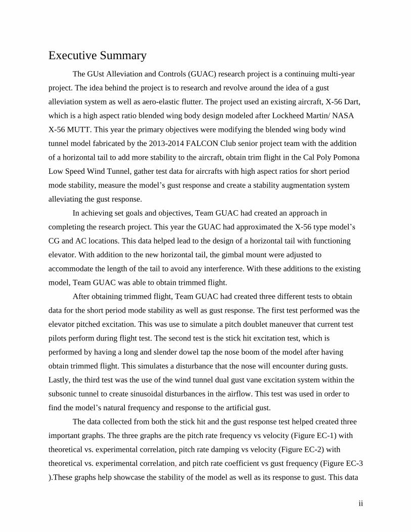
Executive Summary
The GUst Alleviation and Controls (GUAC) research project is a continuing multi-year
project. The idea behind the project is to research and revolve around the idea of a gust
alleviation system as well as aero-elastic flutter. The project used an existing aircraft, X-56 Dart,
which is a high aspect ratio blended wing body design modeled after Lockheed Martin/ NASA
X-56 MUTT. This year the primary objectives were modifying the blended wing body wind
tunnel model fabricated by the 2013-2014 FALCON Club senior project team with the addition
of a horizontal tail to add more stability to the aircraft, obtain trim flight in the Cal Poly Pomona
Low Speed Wind Tunnel, gather test data for aircrafts with high aspect ratios for short period
mode stability, measure the model’s gust response and create a stability augmentation system
alleviating the gust response.
In achieving set goals and objectives, Team GUAC had created an approach in
completing the research project. This year the GUAC had approximated the X-56 type model’s
CG and AC locations. This data helped lead to the design of a horizontal tail with functioning
elevator. With addition to the new horizontal tail, the gimbal mount were adjusted to
accommodate the length of the tail to avoid any interference. With these additions to the existing
model, Team GUAC was able to obtain trimmed flight.
After obtaining trimmed flight, Team GUAC had created three different tests to obtain
data for the short period mode stability as well as gust response. The first test performed was the
elevator pitched excitation. This was use to simulate a pitch doublet maneuver that current test
pilots perform during flight test. The second test is the stick hit excitation test, which is
performed by having a long and slender dowel tap the nose boom of the model after having
obtain trimmed flight. This simulates a disturbance that the nose will encounter during gusts.
Lastly, the third test was the use of the wind tunnel dual gust vane excitation system within the
subsonic tunnel to create sinusoidal disturbances in the airflow. This test was used in order to
find the model’s natural frequency and response to the artificial gust.
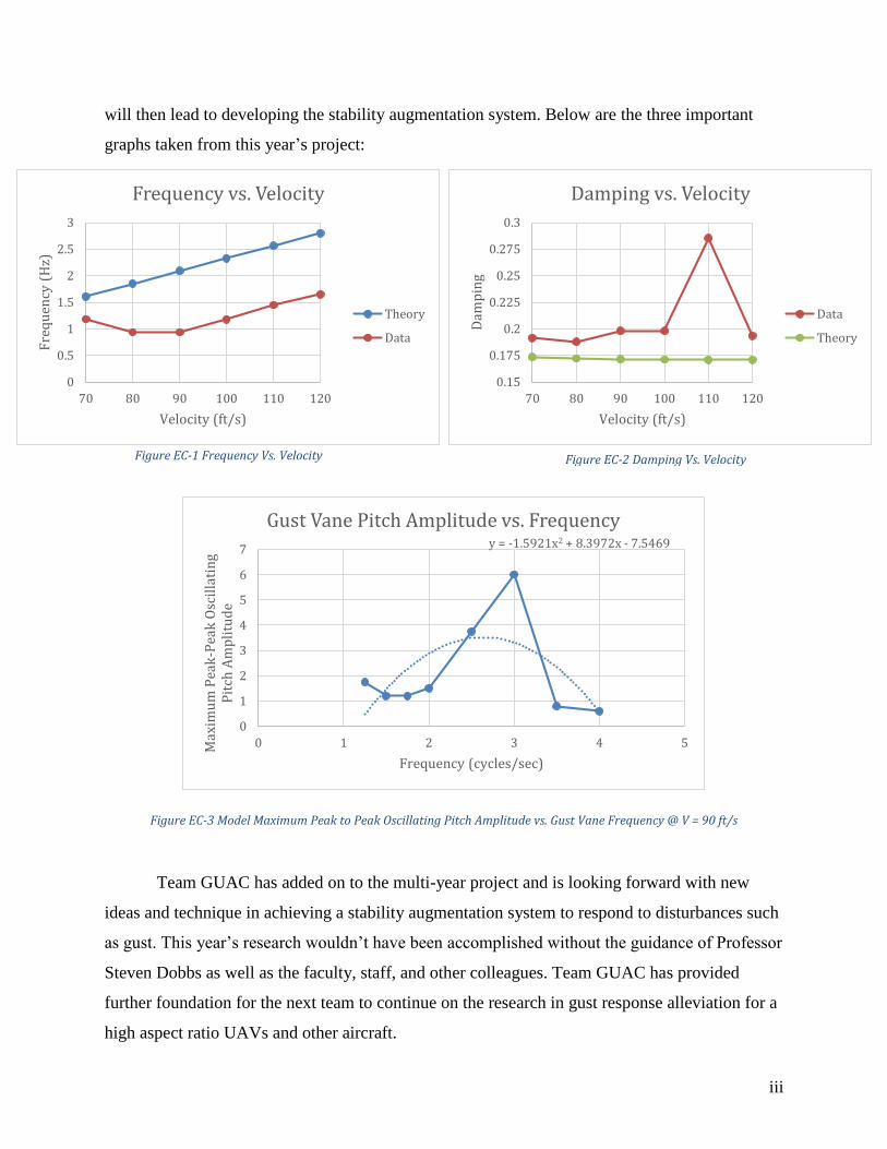
The data collected from both the stick hit and the gust response test helped created three
important graphs. The three graphs are the pitch rate frequency vs velocity (Figure EC-1) with
theoretical vs. experimental correlation, pitch rate damping vs velocity (Figure EC-2) with
theoretical vs. experimental correlation, and pitch rate coefficient vs gust frequency (Figure EC-3
).These graphs help showcase the stability of the model as well as its response to gust. This data
iii
will then lead to developing the stability augmentation system. Below are the three important
graphs taken from this year’s project:
Figure EC-3 Model Maximum Peak to Peak Oscillating Pitch Amplitude vs. Gust Vane Frequency @ V = 90 ft/s
Team GUAC has added on to the multi-year project and is looking forward with new
ideas and technique in achieving a stability augmentation system to respond to disturbances such
as gust. This year’s research wouldn’t have been accomplished without the guidance of Professor
Steven Dobbs as well as the faculty, staff, and other colleagues. Team GUAC has provided
further foundation for the next team to continue on the research in gust response alleviation for a
high aspect ratio UAVs and other aircraft.
y = -1.5921x2 + 8.3972x - 7.5469
0
1
2
3
4
5
6
7
0 1 2 3 4 5Max
imu
m P
eak
-Pea
k O
scil
lati
ng
Pit
ch A
mp
litu
de
Frequency (cycles/sec)
Gust Vane Pitch Amplitude vs. Frequency
0
0.5
1
1.5
2
2.5
3
70 80 90 100 110 120
Fre
qu
ency
(H
z)
Velocity (ft/s)
Frequency vs. Velocity
Theory
Data
0.15
0.175
0.2
0.225
0.25
0.275
0.3
70 80 90 100 110 120
Dam
pin
g
Velocity (ft/s)
Damping vs. Velocity
Data
Theory
Figure EC-1 Frequency Vs. Velocity Figure EC-2 Damping Vs. Velocity
iv
Table of Contents
1.0 Introduction ........................................................................................................................ 12
1.1 Needs Analysis and Problem Statement......................................................................... 12
1.2 Project Objectives .......................................................................................................... 13
1.3 Project Approach ............................................................................................................ 14
2.0 Systems Engineering .......................................................................................................... 15
2.1 Team Organization ......................................................................................................... 15
2.2 Needs .............................................................................................................................. 16
2.3 Program Objectives ........................................................................................................ 16
2.4 Schedule ......................................................................................................................... 17
2.5 Project Budget ................................................................................................................ 19
3.0 X-56 Type Design .............................................................................................................. 20
4.0 X-56 Type Fabrication and Assembly ............................................................................... 21
4.1 Fuselage .......................................................................................................................... 21
4.1.1 Material Used .......................................................................................................... 21
4.1.2 Fuselage Fabrication ............................................................................................... 21
4.1.3 X-56 Type Styrofoam Base Repair ......................................................................... 21
4.1.4 Nose Boom with Movable Weight (See Section 5.4) ............................................. 23
4.2 Horizontal Tail ............................................................................................................... 23
4.2.1 Horizontal Tail Fabrication ..................................................................................... 23
4.3 Gimbal and Sting ............................................................................................................ 26
4.3.1 Gimbal Fabrication and Modification ..................................................................... 26
4.3.2 Sting Modification .................................................................................................. 29
5.0 Testing And Preparation .................................................................................................... 30
5.1 X-56 Model Installation On Tunnel Sting With Gimbal Mount (See Reference) ......... 30
5.1.1 X-56 Model Installation Procedure ......................................................................... 30
5.1.2 Model Longitudinal Stability Test Procedures ....................................................... 30
v
5.1.2.1 Longitudinal Stability Frequency and Pitch Damping Test ............................ 30
5.1.2.1.1 Pulse Excitation Method Procedure ..................................................................... 30
5.1.2.1.2 Stick-Hit-Nose Boom Excitation Method Procedure ..................................... 31
5.1.3 Test Results (See Section 9.1.2) ............................................................................. 31
5.2 Gust Vane System Installation (See Reference) ............................................................ 32
5.2.1 Test Equipment (See Reference) ............................................................................ 32
5.2.2 Gust Vane Operation Procedure For Varying Vane Frequency and Oscillation
Angle Amplitude ................................................................................................................... 32
5.2.3 Test Plan (See Appendix) ....................................................................................... 32
5.2.4 Test Results (See Section 9) ................................................................................... 32
5.3 Aerodynamic Center Testing and Results ...................................................................... 33
5.3.1 Analysis Procedure ................................................................................................. 33
5.3.2 Test Results ............................................................................................................. 33
5.4 Center of Gravity Testing ............................................................................................... 36
5.4.1 Test Procedures ....................................................................................................... 36
5.4.2 Test Results ............................................................................................................. 38
................................................................................................................................................... 39
5.6 Static Wing Loading Test And Results .......................................................................... 40
5.6.1 Test Procedure ........................................................................................................ 40
5.6.2 Test Results ............................................................................................................. 43
6.0 Theory Predictions Using Athena Vortex Lattice (AVL) .................................................. 45
6.1 Theory Predictions of Models Aerodynamic Center Vs. Center Of Gravity Using
Athena Vortex Lattice (AVL) ................................................................................................... 45
6.3 Theory Predictions Of Model Stability Derivatives Using Athena Vortex Lattice (AVL)
47
7.0 Simulink Real-Time Control System: (See Reference) ..................................................... 49
7.1 Simulink Model Configuration: (See Reference)........................................................... 49
vi
7.2 The Real-Time Windows Target: (See Reference) ........................................................ 49
7.2.1 Advantages of the Real-Time Windows Target (See Reference) ........................... 49
7.2.2 Known Issues with the Real-Time Windows Target (See Reference) ................... 49
7.3 The X-56 DART Flight Controls Model: (See Reference) ............................................ 49
7.3.1 The ArduPilot Mega(APM) Interface Subsystem (See Reference) ........................ 49
7.3.2 Pilot Input Subsystem (See Reference) ................................................................... 49
7.3.3 The System Status Subsystem (See Reference) ...................................................... 49
7.3.4 The Wind Tunnel Data Recorder Subsystem (See Reference) ............................... 49
8.0 Wind Tunnel Data Acquisition and Analysis .................................................................... 50
8.1 Wind Tunnel Test Data Acquisition (See Reference) .................................................... 50
8.2 Wind Test Data Analysis Method (See Reference) ....................................................... 50
8.2.1 Longitudinal Stability Tests Example Calculations (See Reference) ..................... 50
8.2.2 Gust Response Test Example Calculations............................................................. 50
9.0 Wind Tunnel Test Results .................................................................................................. 51
9.1 Longitudinal Stability Frequency And Pitch Damping Test .......................................... 51
9.1.1 Elevator Pulse Excitation Method Results .............................................................. 51
9.1.2 Stick-Hit-Nose Boom Excitation Method Results .................................................. 51
9.2 Gust Response Magnitude vs. Gust Vane Deflection And Frequency Test- Gust
Response Magnitude vs. Vane Frequency At Various Tunnel Velocities ................................ 52
9.2.1 Test Results ............................................................................................................. 52
9.2.2 Finding Natural Frequency through Gust Response Analysis ................................ 55
9.3 Error and Problems......................................................................................................... 56
10.0 Conclusion ......................................................................................................................... 57
11.0 Recommendation ............................................................................................................... 58
12.0 Contributions and Acknowledgments ................................................................................ 59
13.0 References .......................................................................................................................... 60
13.1 Previous Senior Project Report (Team Falcon by Evan Johnson) ................................. 60
13.2 MATLAT Plots .............................................................................................................. 60
vii
13.2.1 Stick Excitation Test Plots ...................................................................................... 60
13.2.1.1 Velocity at 77 fps ............................................................................................................. 60
13.2.1.2 Velocity at 80 fps ............................................................................................................. 61
13.2.1.3 Velocity at 90 fps ............................................................................................................. 67
13.2.1.4 Velocity at 100 fps .......................................................................................................... 70
13.2.1.5 Velocity at 110 fps .......................................................................................................... 73
13.2.1.6 Velocity at 120 fps .......................................................................................................... 76
13.2.2 Frequency Excitation Plots ..................................................................................... 79
13.2.2.1 Velocity at 80 fps ............................................................................................................. 79
13.2.2.2 Velocity at 90 fps ............................................................................................................. 81
13.2.2.3 Velocity at 100 fps .......................................................................................................... 83
13.3 Excel Data Results ......................................................................................................... 86
13.3.1 Stick Excitation Test ............................................................................................... 86
13.3.1.1 Velocity at 77 fps ............................................................................................................. 86
13.3.1.2 Velocity at 80 fps ............................................................................................................. 86
13.3.1.3 Velocity at 90 fps ............................................................................................................. 86
13.3.1.4 Velocity at 100 fps .......................................................................................................... 87
13.3.1.5 Velocity at 110 fps .......................................................................................................... 87
13.3.1.6 Velocity at 120 fps .......................................................................................................... 87
13.4 Books .............................................................................................................................. 88
13.5 Other Documents............................................................................................................ 88
13.6 Poster Copy .................................................................................................................... 89
Appendix A-1: Code Listing ........................................................................................................ 90
A-1.1 Matlab Code for short period approximation .................................................................. 90
Appendix A-2: AVL Input Files .................................................................................................. 91
viii
A-2.1 Geometry File (.avl) ........................................................................................................ 91
A-2.2 Run Case File .................................................................................................................. 95
A-2.3 Airfoil Geometry File: Fuselage.dat ............................................................................... 96
A-2.4 Airfoil Geometry File: Wing.dat ..................................................................................... 99
Appendix A-3: Proposal ............................................................................................................. 102
Appendix A-4: Stick Excitation Test Plan .................................................................................. 110
ix
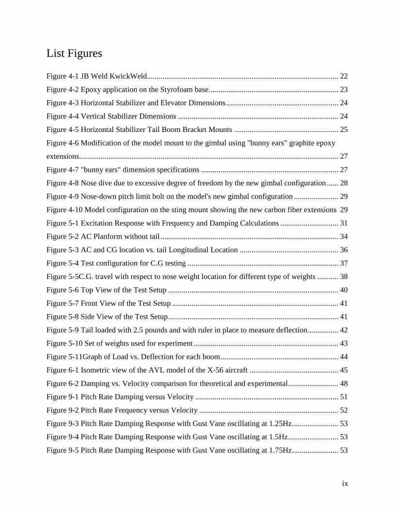
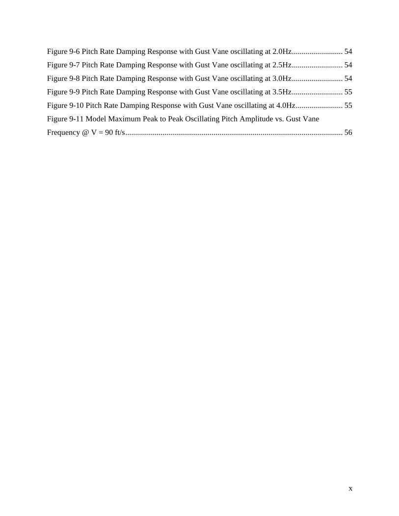
List Figures
Figure 4-1 JB Weld KwickWeld................................................................................................... 22
Figure 4-2 Epoxy application on the Styrofoam base. .................................................................. 23
Figure 4-3 Horizontal Stabilizer and Elevator Dimensions .......................................................... 24
Figure 4-4 Vertical Stabilizer Dimensions ................................................................................... 24
Figure 4-5 Horizontal Stabilizer Tail Boom Bracket Mounts ...................................................... 25
Figure 4-6 Modification of the model mount to the gimbal using "bunny ears" graphite epoxy
extensions ...................................................................................................................................... 27
Figure 4-7 "bunny ears" dimension specifications ....................................................................... 27
Figure 4-8 Nose dive due to excessive degree of freedom by the new gimbal configuration ...... 28
Figure 4-9 Nose-down pitch limit bolt on the model's new gimbal configuration ....................... 29
Figure 4-10 Model configuration on the sting mount showing the new carbon fiber extensions 29
Figure 5-1 Excitation Response with Frequency and Damping Calculations .............................. 31
Figure 5-2 AC Planform without tail ............................................................................................ 34
Figure 5-3 AC and CG location vs. tail Longitudinal Location ................................................... 36
Figure 5-4 Test configuration for C.G testing .............................................................................. 37
Figure 5-5C.G. travel with respect to nose weight location for different type of weights ........... 38
Figure 5-6 Top View of the Test Setup ........................................................................................ 40
Figure 5-7 Front View of the Test Setup ...................................................................................... 41
Figure 5-8 Side View of the Test Setup ........................................................................................ 41
Figure 5-9 Tail loaded with 2.5 pounds and with ruler in place to measure deflection ................ 42
Figure 5-10 Set of weights used for experiment ........................................................................... 43
Figure 5-11Graph of Load vs. Deflection for each boom ............................................................. 44
Figure 6-1 Isometric view of the AVL model of the X-56 aircraft .............................................. 45
Figure 6-2 Damping vs. Velocity comparison for theoretical and experimental .......................... 48
Figure 9-1 Pitch Rate Damping versus Velocity .......................................................................... 51
Figure 9-2 Pitch Rate Frequency versus Velocity ........................................................................ 52
Figure 9-3 Pitch Rate Damping Response with Gust Vane oscillating at 1.25Hz ........................ 53
Figure 9-4 Pitch Rate Damping Response with Gust Vane oscillating at 1.5Hz .......................... 53
Figure 9-5 Pitch Rate Damping Response with Gust Vane oscillating at 1.75Hz ........................ 53
x
Figure 9-6 Pitch Rate Damping Response with Gust Vane oscillating at 2.0Hz .......................... 54
Figure 9-7 Pitch Rate Damping Response with Gust Vane oscillating at 2.5Hz .......................... 54
Figure 9-8 Pitch Rate Damping Response with Gust Vane oscillating at 3.0Hz .......................... 54
Figure 9-9 Pitch Rate Damping Response with Gust Vane oscillating at 3.5Hz .......................... 55
Figure 9-10 Pitch Rate Damping Response with Gust Vane oscillating at 4.0Hz ........................ 55
Figure 9-11 Model Maximum Peak to Peak Oscillating Pitch Amplitude vs. Gust Vane
Frequency @ V = 90 ft/s ............................................................................................................... 56
xi
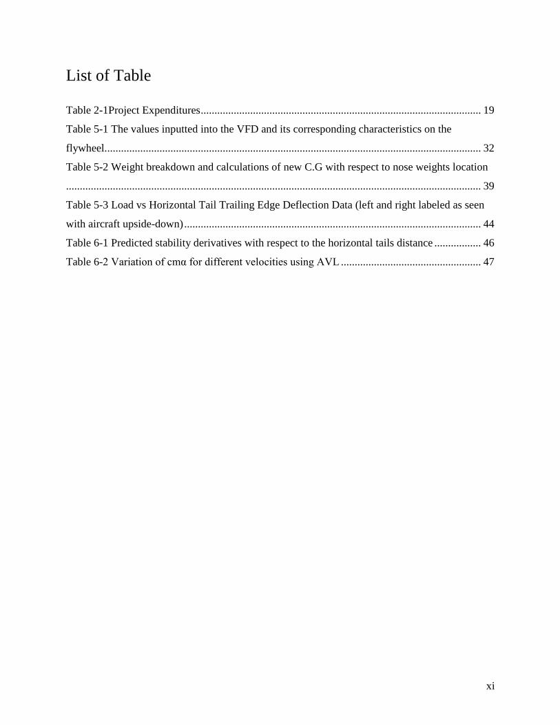
List of Table
Table 2-1Project Expenditures ...................................................................................................... 19
Table 5-1 The values inputted into the VFD and its corresponding characteristics on the
flywheel......................................................................................................................................... 32
Table 5-2 Weight breakdown and calculations of new C.G with respect to nose weights location
....................................................................................................................................................... 39
Table 5-3 Load vs Horizontal Tail Trailing Edge Deflection Data (left and right labeled as seen
with aircraft upside-down) ............................................................................................................ 44
Table 6-1 Predicted stability derivatives with respect to the horizontal tails distance ................. 46
Table 6-2 Variation of cmα for different velocities using AVL ................................................... 47
12
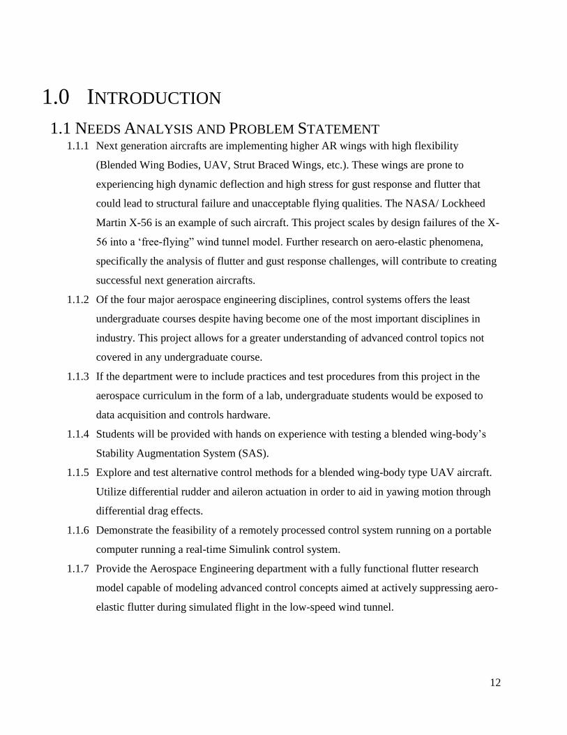
1.0 INTRODUCTION
1.1 NEEDS ANALYSIS AND PROBLEM STATEMENT 1.1.1 Next generation aircrafts are implementing higher AR wings with high flexibility
(Blended Wing Bodies, UAV, Strut Braced Wings, etc.). These wings are prone to
experiencing high dynamic deflection and high stress for gust response and flutter that
could lead to structural failure and unacceptable flying qualities. The NASA/ Lockheed
Martin X-56 is an example of such aircraft. This project scales by design failures of the X-
56 into a ‘free-flying” wind tunnel model. Further research on aero-elastic phenomena,
specifically the analysis of flutter and gust response challenges, will contribute to creating
successful next generation aircrafts.
1.1.2 Of the four major aerospace engineering disciplines, control systems offers the least
undergraduate courses despite having become one of the most important disciplines in
industry. This project allows for a greater understanding of advanced control topics not
covered in any undergraduate course.
1.1.3 If the department were to include practices and test procedures from this project in the
aerospace curriculum in the form of a lab, undergraduate students would be exposed to
data acquisition and controls hardware.
1.1.4 Students will be provided with hands on experience with testing a blended wing-body’s
Stability Augmentation System (SAS).
1.1.5 Explore and test alternative control methods for a blended wing-body type UAV aircraft.
Utilize differential rudder and aileron actuation in order to aid in yawing motion through
differential drag effects.
1.1.6 Demonstrate the feasibility of a remotely processed control system running on a portable
computer running a real-time Simulink control system.
1.1.7 Provide the Aerospace Engineering department with a fully functional flutter research
model capable of modeling advanced control concepts aimed at actively suppressing aero-
elastic flutter during simulated flight in the low-speed wind tunnel.
13
1.2 PROJECT OBJECTIVES 1.2.1 Modifying the blended wing body model fabricated by the 2013-2014 FALCON Club
senior project team. The modified scale model of the X-56 will have a relocated C.G by
the use of a nose boom weight in front of the model. The goal of this is to move the AC aft
of the C.G. for static and dynamic stability.
1.2.2 The FALCON (Flutter ALleviation and CONtrol) model will be tested in the subsonic
wind tunnel with two degrees of freedom for longitudinal stability testing in order to
develop an optimized longitudinal Stability Augmentation control system.
1.2.3 Demonstrate a longitudinal gust alleviation system capable of reacting to vertical gusts in
the subsonic wind tunnel. This test will utilize the gust generation system designed and
installed in the wind tunnel by the 2012-2013 Flutter Club team.
1.2.4 Expand stability augmentation system to include lateral-directional motion. Demonstrate
controllability and augmented static and dynamic stability of a blended wing-body aircraft
in five degree of freedom motion.
1.2.5 Super impose the stability augmentation system with gust alleviation system to reduce
flutter phenomena for a rigid wing structure.
1.2.6 Perform preliminary vibration and flutter analysis in NASTRAN for a composite-skinned
flexible wing optimized for span wise torsional bending. Determine optimal material,
wing structure, and mass distribution to obtain desired structural dynamic modes.
14
1.3 PROJECT APPROACH 1.3.1 Approximate X-56 type model CG and AC locations. Design tail that will move AC
further back while not affecting CG location. Use light material for tail
1.3.2 Create Horizontal Tail with RC controlled elevator for enhanced trim control and
longitudinal stability to add to Existing X-56 Model
1.3.3 Add functioning elevator to control pitch
1.3.4 Lock wingtip rudders
1.3.5 Use Cal Poly Low Speed Wind Tunnel to achieve stable flight
1.3.6 Attach model to gimbal mount, then attach model/gimbal mount apparatus to crescent
sting in order to simulate free flight in pitch and plunge.
1.3.7 Use Team Falcon’s Simulink model in order to control model with joystick
1.3.8 Use the on board gyros and accelerometer to measure pitch, pitch rate, and time
1.3.9 Simulate turbulent wind conditions by fluctuating the model in pitch. This can be
accomplished by performing an elevator pulse-doublet as well as by tapping the nose
boom with a rod.
1.3.10 Vary gust vanes frequency in the tunnel in order to find the model’s natural short period
frequency and maximum response amplitude for future use in designing a gust alleviation
system
15
2.0 SYSTEMS ENGINEERING
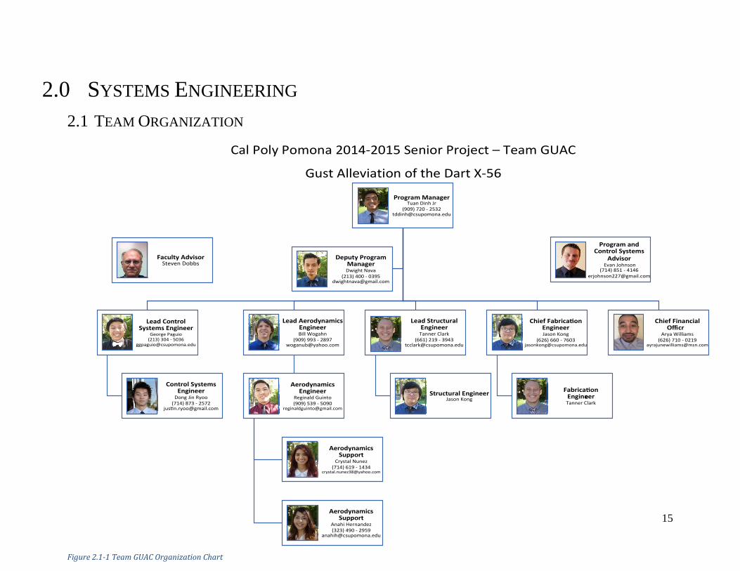
2.1 TEAM ORGANIZATION
ProgramManagerTuanDinhJr
(909)[email protected]
LeadControlSystemsEngineer
GeorgePaguio(213)304-5036
ControlSystemsEngineer
DongJinRyoo(714)873-2572
LeadAerodynamicsEngineerBillWogahn
(909)[email protected]
AerodynamicsEngineer
ReginaldGuinto(909)539-5090
AerodynamicsSupport
CrystalNunez(714)619-1434
AerodynamicsSupport
AnahiHernandez(323)490-2959
LeadStructuralEngineerTannerClark
(661)[email protected]
StructuralEngineerJasonKong
ChiefFabrica onEngineerJasonKong
(626)[email protected]
Fabrica onEngineerTannerClark
ChiefFinancialOffic
e
r
AryaWilliams(626)710-0219
DeputyProgramManagerDwightNava
(213)[email protected]
ProgramandControlSystems
AdvisorEvanJohnson(714)851-4146
FacultyAdvisorStevenDobbs
CalPolyPomona2014-2015SeniorProject–TeamGUAC
GustAlleviationoftheDartX-56
Figure 2.1-1 Team GUAC Organization Chart
16
2.2 NEEDS Research towards flutter alleviation of blended wing bodies is few and far between. The
study of gust alleviation and stability augmentation systems of blended wing bodies is to this day
one of the subjects being actively studied in industry today.
For the team, this projects provides team members with the opportunity to be exposed to the
systems engineering process. By integrating aerodynamic theory to application and applying the
manufacturing process, students are introduced through the design life cycle and manage the
entire program with the principles of system engineering.
2.3 PROGRAM OBJECTIVES This is a multi-year research opportunity exploring the control alleviation of gusts of
blended wing bodies. For the fourth year iteration of the project, the goal of the GUAC Team is
to make the aircraft Aerodynamically Stable. Previous year’s design had the center of gravity aft
the aerodynamic center which contributed to its stability issues. To correct these issues GUAC
will modify the design by incorporating a twin-boom tail, including a new elevator and two new
rudders to the aft section of the model. Thus correcting model’s stability issues.
By developing a stability as well as a gust alleviation system for a rigid wing model, this
provides a baseline to explore other autopilot and stability augmentation systems of flexible
systems for future teams to research. The mechanics to control the magnitude of the gust had
been set in place. However the capabilities of the gust-vane system had not been measured and
thus after the previous year had just finished constructing the gust-vane system and to pick up
from last year, the gust-vane system flow dynamics must be characterized.
17
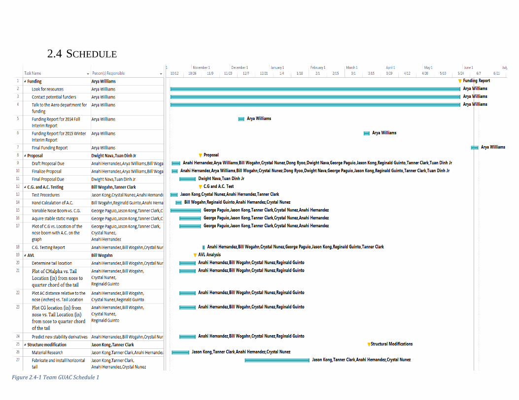
2.4 SCHEDULE
Figure 2.4-1 Team GUAC Schedule 1
18
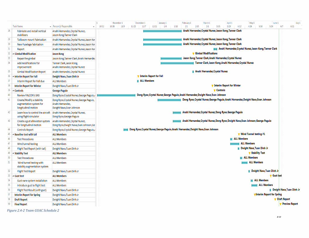
Figure 2.4-2 Team GUAC Schedule 2
19
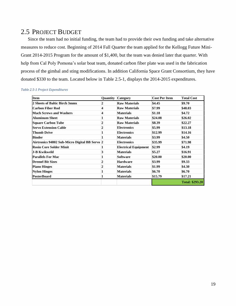
2.5 PROJECT BUDGET Since the team had no initial funding, the team had to provide their own funding and take alternative
measures to reduce cost. Beginning of 2014 Fall Quarter the team applied for the Kellogg Future Mini-
Grant 2014-2015 Program for the amount of $1,400, but the team was denied later that quarter. With
help from Cal Poly Pomona’s solar boat team, donated carbon fiber plate was used in the fabrication
process of the gimbal and sting modifications. In addition California Space Grant Consortium, they have
donated $330 to the team. Located below in Table 2.5-1, displays the 2014-2015 expenditures.
Table 2.5-1 Project Expenditures
Item Quantity Category Cost Per Item Total Cost
2 Sheets of Baltic Birch 3mmx 2 Raw Materials $4.45 $9.70
Carbon Fiber Rod 4 Raw Materials $7.99 $48.03
Mach Screws and Washers 4 Materials $1.18 $4.72
Aluminum Sheet 1 Raw Materials $24.08 $26.02
Square Carbon Tube 2 Raw Materials $8.39 $22.27
Servo Extension Cable 2 Electronics $5.99 $13.18
Thumb Drive 1 Electronics $12.99 $14.16
Binder 1 Materials $3.99 $4.50
Airtronics 94802 Sub-Micro Digital BB Servo 2 Electronics $35.99 $71.98
Rosin Core Solder Minit 1 Electrical Equipment $2.99 $4.19
J-B Kwikweld 3 Materials $5.27 $16.91
Parallels For Mac 1 Software $20.00 $20.00
Dremel Bit Sizes 2 Hardware $3.99 $9.33
Piano Hinges 2 Materials $1.99 $4.30
Nylon Hinges 1 Materials $6.70 $6.70
PosterBoard 1 Materials $15.79 $17.21
Total: $293.20
20
3.0 X-56 TYPE DESIGN After the center of gravity and the aerodynamic center of the X-56 were located, it was discovered
that the reason the model was unstable in previous wind tunnel tests was because of the location of the
aerodynamic center with respect to the center of gravity. The best way to correct this problem and move
the aerodynamic center was to install a horizontal tail using two booms, which would be installed to the
body of the aircraft. It was determined that the body of the model has to be modified in order to make
room for the two booms as well as the assembly to hold the booms. This modification is done by carving
out some of the foam in the shape of the aluminum “U” brackets on the interior of the bottom half of the
body using a Dremel Rotary Tool. The back of the body will also have to be carved out in order for the
booms to protrude from the back of the aircraft. After the body is shaped to attach the tail booms, all
rough edges will be sanded down in order to create a smooth surface for the air to flow over during the
wind tunnel testing.
While these modifications are being done to the fuselage, the CAD model of the fuselage will be
modified in order to create a new fuselage, which would allow for the tail booms. After the CAD model
is modified, a 3-D printer will be used to create a negative of the base. This negative will then be used to
create a mold of the body of the aircraft. Using this mold, a solid base can then be created using the
same material as the original body for consistency. After the mold is completed, the exterior will be
sanded down to create as smooth of a surface as possible for the air to flow over it. However, fabrication
of this new fuselage was not performed in this project.
21
4.0 X-56 TYPE FABRICATION AND ASSEMBLY
4.1 FUSELAGE For an aircraft to be aerodynamically stable, its aerodynamic center should be located behind the
center of gravity. However, in the X-56’s current design and configuration, the center of gravity is well
aft of the aerodynamic center by about 2.25”. In order for the aircraft to become aerodynamically stable,
the proposal is to incorporate a twin-boom tail, including a new elevator and two new rudders, to the aft
section of the aircraft. This in turn should help shift the aerodynamic center of the aircraft aft and help
with aircraft stability.
4.1.1 Material Used
2 Carbon fiber rods, minimum of 18” in length and 3/8” in diameter
1 medium-sized birch plywood board, 1/16” thick
2 Airtronics 94802 Sub-Micro Digital BB Servos
Actuators (2 rudders and 1 elevator)
4.1.2 Fuselage Fabrication Two carbon-fiber square rods have been purchased from Rockwest Composites, each stick
measuring 2 feet in length and 3/8th inches in diameter. A piece of birch plywood measuring 1/16” thick
was also purchased for crafting the new vertical and horizontal stabilizers and twin vertical tails. The
two booms will be internally mounted to the aircraft’s carbon fiber skeleton via four aluminum “u”
bracket mounts, two on either side of the aircraft. The booms will be able to slide along its mount to a
specified length based on performance, and can be held in place with a lock screw. Since there are new
protrusions coming out of the aircraft’s fuselage, the current Styrofoam base of the fuselage either needs
to be remade or modified to fit the new tail booms while maintaining the aircraft’s aerodynamics.
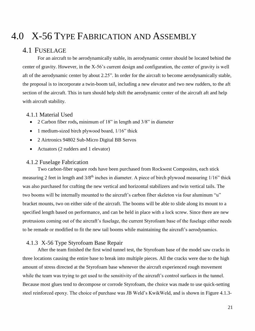
4.1.3 X-56 Type Styrofoam Base Repair After the team finished the first wind tunnel test, the Styrofoam base of the model saw cracks in
three locations causing the entire base to break into multiple pieces. All the cracks were due to the high
amount of stress directed at the Styrofoam base whenever the aircraft experienced rough movement
while the team was trying to get used to the sensitivity of the aircraft’s control surfaces in the tunnel.
Because most glues tend to decompose or corrode Styrofoam, the choice was made to use quick-setting
steel reinforced epoxy. The choice of purchase was JB Weld’s KwikWeld, and is shown in Figure 4.1.3-
22
1 below. The epoxy sets in about four minutes and cures in approximately 4 hours; with a listed shear
strength of 2424 psi.
Figure 4-1 JB Weld KwickWeld
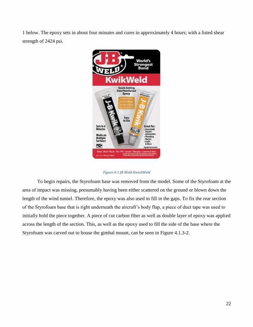
To begin repairs, the Styrofoam base was removed from the model. Some of the Styrofoam at the
area of impact was missing, presumably having been either scattered on the ground or blown down the
length of the wind tunnel. Therefore, the epoxy was also used to fill in the gaps. To fix the rear section
of the Styrofoam base that is right underneath the aircraft’s body flap, a piece of duct tape was used to
initially hold the piece together. A piece of cut carbon fiber as well as double layer of epoxy was applied
across the length of the section. This, as well as the epoxy used to fill the side of the base where the
Styrofoam was carved out to house the gimbal mount, can be seen in Figure 4.1.3-2.
23
Figure 4-2 Epoxy application on the Styrofoam base.
To ensure that the double layer of epoxy was fully set, the Styrofoam base was left untouched for 24
hours, and was then reattached to the model the following day. Tests were subsequently performed for
the rest of the week without incident, and no further stress cracks were noticed on the repaired base.
4.1.4 Nose Boom with Movable Weight (See Section 5.4)
4.2 HORIZONTAL TAIL
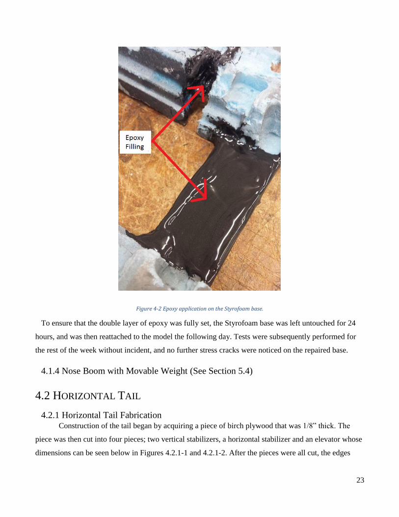
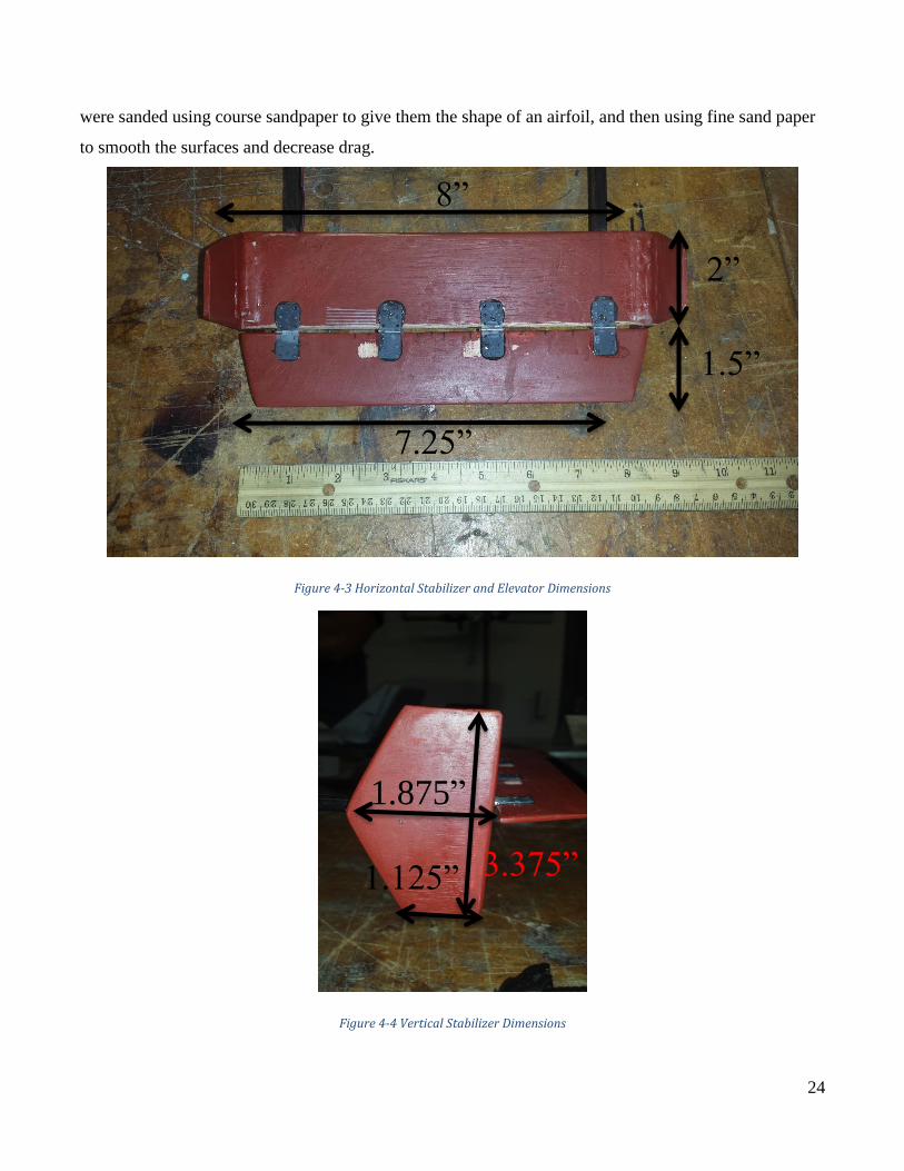
4.2.1 Horizontal Tail Fabrication Construction of the tail began by acquiring a piece of birch plywood that was 1/8” thick. The
piece was then cut into four pieces; two vertical stabilizers, a horizontal stabilizer and an elevator whose
dimensions can be seen below in Figures 4.2.1-1 and 4.2.1-2. After the pieces were all cut, the edges
24
were sanded using course sandpaper to give them the shape of an airfoil, and then using fine sand paper
to smooth the surfaces and decrease drag.
Figure 4-3 Horizontal Stabilizer and Elevator Dimensions
Figure 4-4 Vertical Stabilizer Dimensions
8”
7.25”
2”
1.5”
1.125”
1.875”
3.375”
25
The assembled tail was then coated with a wood primer and painted. After the paint dried, the
pieces were sanded again and repainted to make the surfaces as smooth as possible. While the tail was
drying for the final time, the tail booms were constructed. A piece of ¼” carbon square tubing was cut
into two 24” long pieces. From there, the two square carbon tubes were measured out so that the new tail
would not collide with the wind tunnel sting mount, but long enough to assist in shifting the
aerodynamic center back as well as providing a bigger moment arm for the control surfaces on the new
tail. To mount the booms, aluminum brackets were molded from strips of sheet aluminum. Holes were
drilled into the carbon-fiber skeleton of the model, and the aluminum brackets were mounted onto the
body. The carbon tubes were then inserted into the brackets and tightened by clamping the brackets with
two bolts on each bracket, one on each side. Two brackets were used for each square carbon tube.
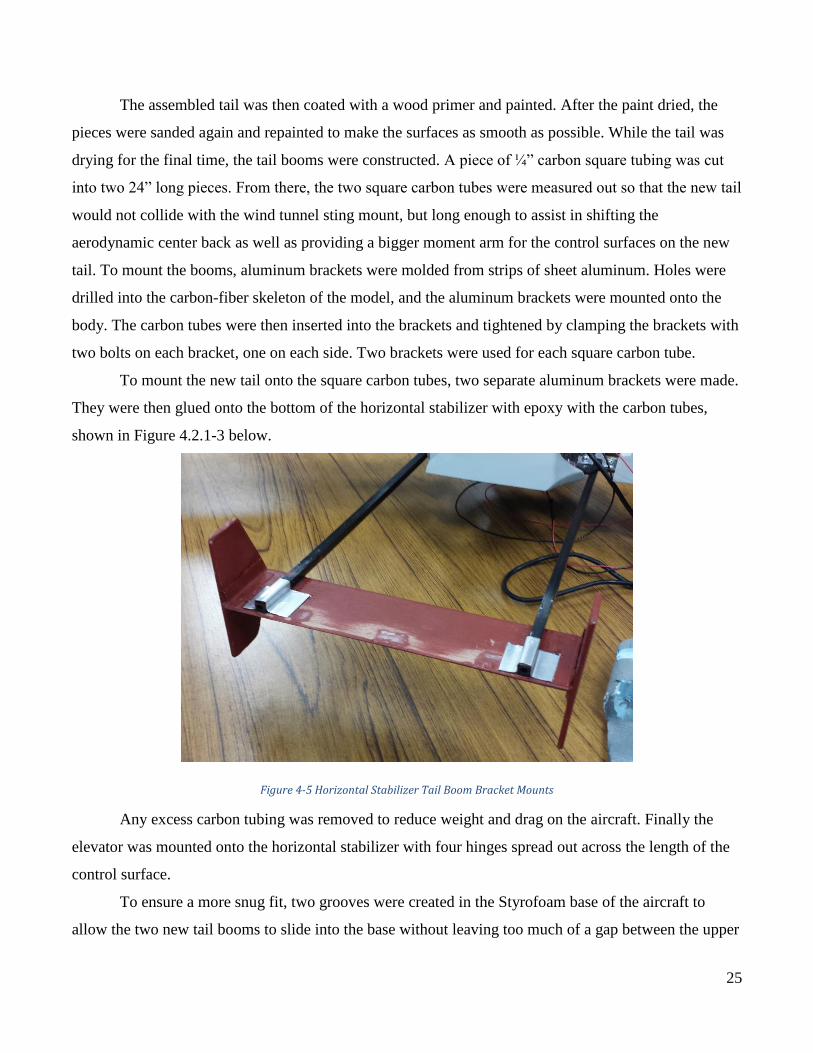
To mount the new tail onto the square carbon tubes, two separate aluminum brackets were made.
They were then glued onto the bottom of the horizontal stabilizer with epoxy with the carbon tubes,
shown in Figure 4.2.1-3 below.
Figure 4-5 Horizontal Stabilizer Tail Boom Bracket Mounts
Any excess carbon tubing was removed to reduce weight and drag on the aircraft. Finally the
elevator was mounted onto the horizontal stabilizer with four hinges spread out across the length of the
control surface.
To ensure a more snug fit, two grooves were created in the Styrofoam base of the aircraft to
allow the two new tail booms to slide into the base without leaving too much of a gap between the upper
26
and lower parts of the fuselage. Finally, a new servo and servo arm was attached to the bottom surface
of the horizontal stabilizer to connect to the new elevator. A small rounded foam mold was made to fit in
front of the servo to minimize drag. The original wire connecting the servo to the Ardupilot was not long
enough, so a 24-inch extension cable was purchased and used to complete the connection.
4.3 GIMBAL AND STING
4.3.1 Gimbal Fabrication and Modification After last year’s recommendation and visual inspection by our advisor this year, we decided that
the gimbal assembly needed to be modified. The gimbal was initially designed for the 3D model of team
prior to the senior project team last year (FALCON). FALCON reused the gimbal was due to time
constraint and machining experience. For this year, no one had machining experience nor found anyone
who could machine a new gimbal, therefore it was decided to just modify the current gimbal.
The first modification made was to find a way to properly mount the gimbal to the frame of the
model. Since the original design accounted for a variable location for the gimbal and we were not able to
reconfigure the model, there was an issue with gap being too far apart for the screws to fit both sides.
This was resolved by using a 4 inch bolt that goes the frame and the gimbal with collars and spacers in
between the two sides. This configuration can be seen in Figure 4.3.1-1. It was secured by putting in two
nuts at the end of the bolt because the vibration would unscrew the nut if it were just one bolt.
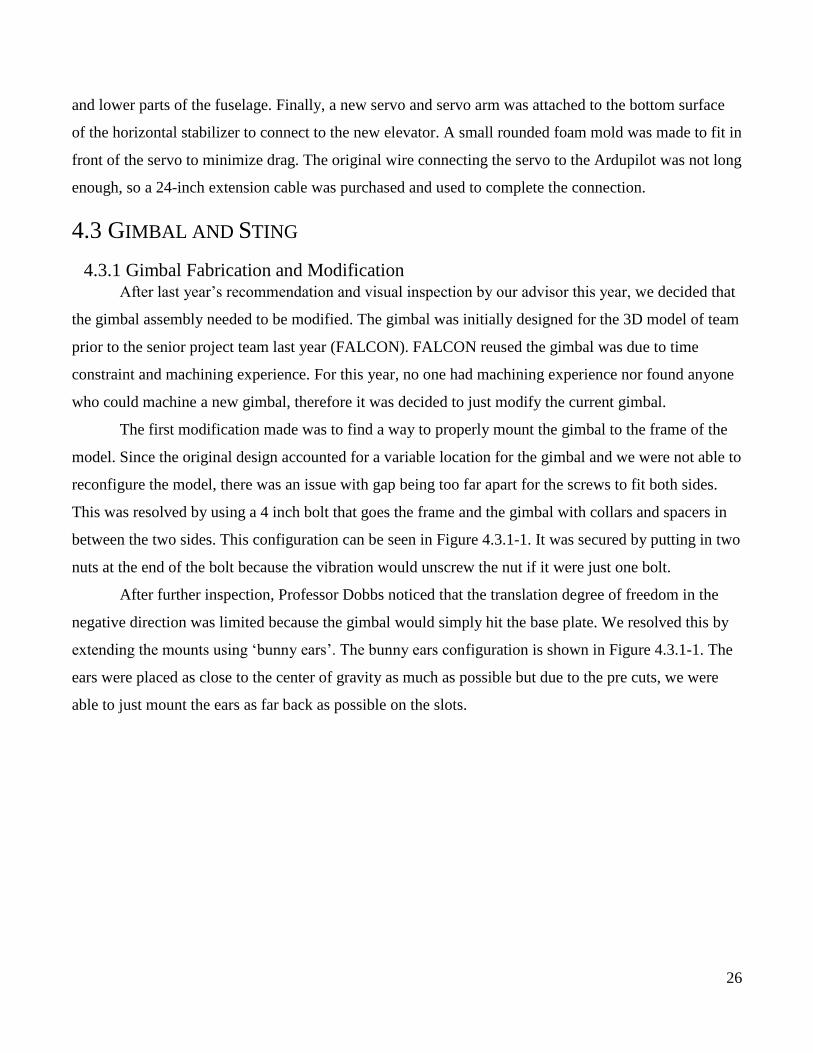
After further inspection, Professor Dobbs noticed that the translation degree of freedom in the
negative direction was limited because the gimbal would simply hit the base plate. We resolved this by
extending the mounts using ‘bunny ears’. The bunny ears configuration is shown in Figure 4.3.1-1. The
ears were placed as close to the center of gravity as much as possible but due to the pre cuts, we were
able to just mount the ears as far back as possible on the slots.
27
Figure 4-6 Modification of the model mount to the gimbal using "bunny ears" graphite epoxy extensions
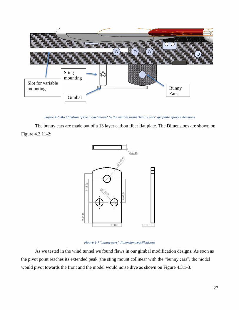
The bunny ears are made out of a 13 layer carbon fiber flat plate. The Dimensions are shown on
Figure 4.3.11-2:
Figure 4-7 "bunny ears" dimension specifications
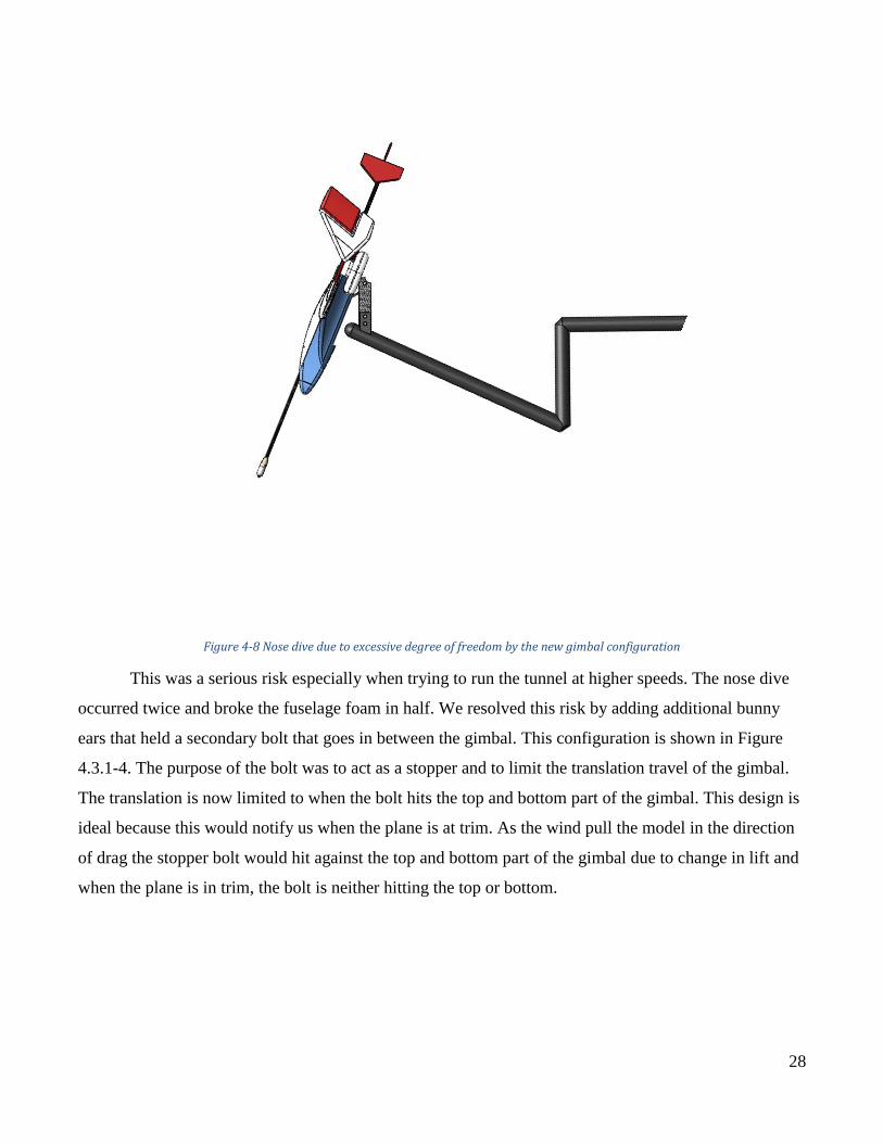
As we tested in the wind tunnel we found flaws in our gimbal modification designs. As soon as
the pivot point reaches its extended peak (the sting mount collinear with the “bunny ears”, the model
would pivot towards the front and the model would noise dive as shown on Figure 4.3.1-3.
Slot for variable
mounting
Gimbal
Sting
mounting
Bunny
Ears
28
Figure 4-8 Nose dive due to excessive degree of freedom by the new gimbal configuration
This was a serious risk especially when trying to run the tunnel at higher speeds. The nose dive
occurred twice and broke the fuselage foam in half. We resolved this risk by adding additional bunny
ears that held a secondary bolt that goes in between the gimbal. This configuration is shown in Figure
4.3.1-4. The purpose of the bolt was to act as a stopper and to limit the translation travel of the gimbal.
The translation is now limited to when the bolt hits the top and bottom part of the gimbal. This design is
ideal because this would notify us when the plane is at trim. As the wind pull the model in the direction
of drag the stopper bolt would hit against the top and bottom part of the gimbal due to change in lift and
when the plane is in trim, the bolt is neither hitting the top or bottom.
29
Figure 4-9 Nose-down pitch limit bolt on the model's new gimbal configuration
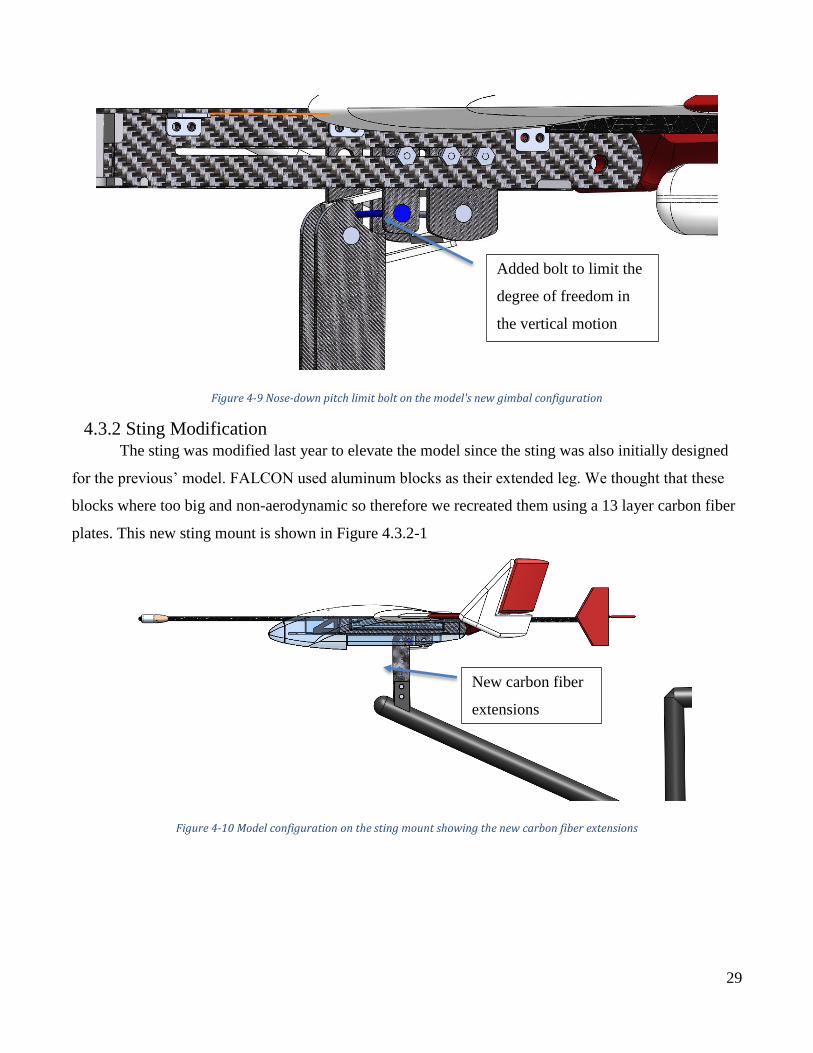
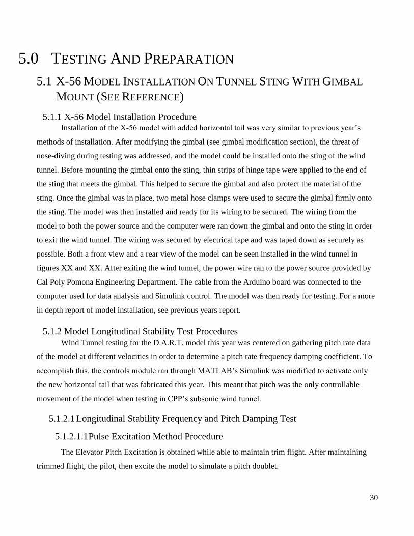
4.3.2 Sting Modification The sting was modified last year to elevate the model since the sting was also initially designed
for the previous’ model. FALCON used aluminum blocks as their extended leg. We thought that these
blocks where too big and non-aerodynamic so therefore we recreated them using a 13 layer carbon fiber
plates. This new sting mount is shown in Figure 4.3.2-1
Figure 4-10 Model configuration on the sting mount showing the new carbon fiber extensions
New carbon fiber
extensions
Added bolt to limit the
degree of freedom in
the vertical motion
30
5.0 TESTING AND PREPARATION
5.1 X-56 MODEL INSTALLATION ON TUNNEL STING WITH GIMBAL
MOUNT (SEE REFERENCE)
5.1.1 X-56 Model Installation Procedure Installation of the X-56 model with added horizontal tail was very similar to previous year’s
methods of installation. After modifying the gimbal (see gimbal modification section), the threat of
nose-diving during testing was addressed, and the model could be installed onto the sting of the wind
tunnel. Before mounting the gimbal onto the sting, thin strips of hinge tape were applied to the end of
the sting that meets the gimbal. This helped to secure the gimbal and also protect the material of the
sting. Once the gimbal was in place, two metal hose clamps were used to secure the gimbal firmly onto
the sting. The model was then installed and ready for its wiring to be secured. The wiring from the
model to both the power source and the computer were ran down the gimbal and onto the sting in order
to exit the wind tunnel. The wiring was secured by electrical tape and was taped down as securely as
possible. Both a front view and a rear view of the model can be seen installed in the wind tunnel in
figures XX and XX. After exiting the wind tunnel, the power wire ran to the power source provided by
Cal Poly Pomona Engineering Department. The cable from the Arduino board was connected to the
computer used for data analysis and Simulink control. The model was then ready for testing. For a more
in depth report of model installation, see previous years report.
5.1.2 Model Longitudinal Stability Test Procedures Wind Tunnel testing for the D.A.R.T. model this year was centered on gathering pitch rate data
of the model at different velocities in order to determine a pitch rate frequency damping coefficient. To
accomplish this, the controls module ran through MATLAB’s Simulink was modified to activate only
the new horizontal tail that was fabricated this year. This meant that pitch was the only controllable
movement of the model when testing in CPP’s subsonic wind tunnel.
5.1.2.1 Longitudinal Stability Frequency and Pitch Damping Test
5.1.2.1.1 Pulse Excitation Method Procedure
The Elevator Pitch Excitation is obtained while able to maintain trim flight. After maintaining
trimmed flight, the pilot, then excite the model to simulate a pitch doublet.
31
5.1.2.1.2 Stick-Hit-Nose Boom Excitation Method Procedure
During testing, the model was trimmed to simulate flight at different velocities. Once set at
stable trim, a pitch pulse was simulated by tapping the nose of the model with a thin and slender rod
through the top slit in the wind tunnel ceiling. This pitch pulse was simulated 6 times at each velocity,
and pitch rate versus time data was gathered through the Arduino board set in the model.
The damping coefficient was determined through Equation 5.1.2.1.2-1:
𝑔 = 1
𝑛𝜋𝐿𝑛(
𝐴𝑜
𝐴𝑛)
Equation 5.1.2.1.2-1
Where n is the number of amplitude cycles within the simulated pitch pulse and 𝐴𝑜 is the
magnitude of the initial amplitude and 𝐴𝑛 in the cycle amplitude at nth cycle this equation was applied
for each of the 6 simulated pitch pulses per velocity. The frequency was calculated by counting the
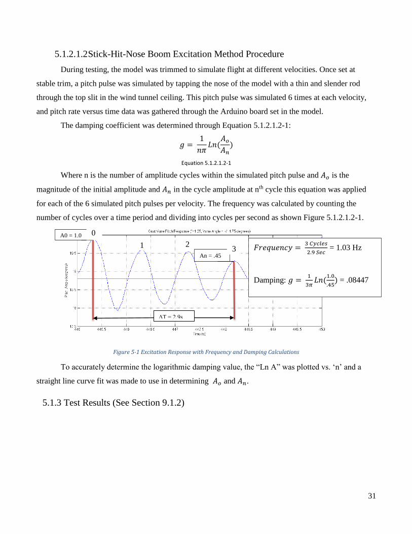
number of cycles over a time period and dividing into cycles per second as shown Figure 5.1.2.1.2-1.
Figure 5-1 Excitation Response with Frequency and Damping Calculations
To accurately determine the logarithmic damping value, the “Ln A” was plotted vs. ‘n’ and a
straight line curve fit was made to use in determining 𝐴𝑜 and 𝐴𝑛.
5.1.3 Test Results (See Section 9.1.2)
ΔT = 2.9s
2 1
An = .45
A0 = 1.0
3 𝐹𝑟𝑒𝑞𝑢𝑒𝑛𝑐𝑦 = 3 𝐶𝑦𝑐𝑙𝑒𝑠
2.9 𝑆𝑒𝑐 = 1.03 Hz
Damping: 𝑔 = 1
3𝜋𝐿𝑛(
1.0
.45) = .08447
0
32
5.2 GUST VANE SYSTEM INSTALLATION (SEE REFERENCE)
5.2.1 Test Equipment (See Reference)
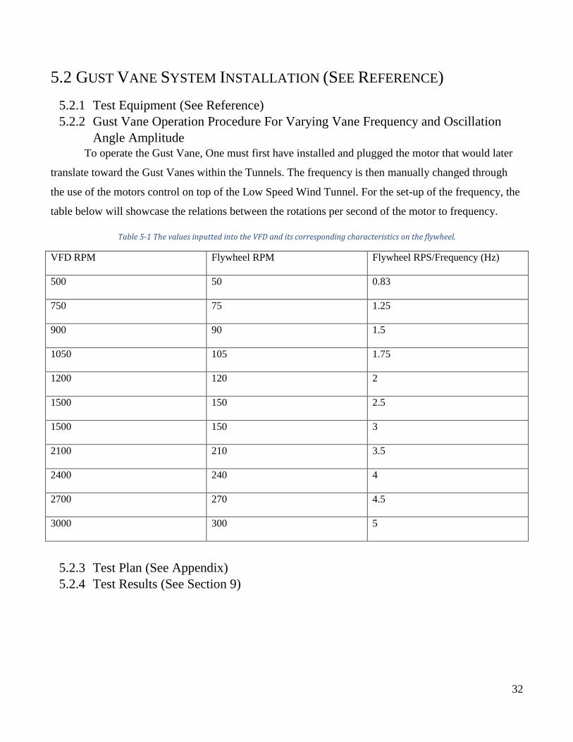
5.2.2 Gust Vane Operation Procedure For Varying Vane Frequency and Oscillation
Angle Amplitude To operate the Gust Vane, One must first have installed and plugged the motor that would later
translate toward the Gust Vanes within the Tunnels. The frequency is then manually changed through
the use of the motors control on top of the Low Speed Wind Tunnel. For the set-up of the frequency, the
table below will showcase the relations between the rotations per second of the motor to frequency.
Table 5-1 The values inputted into the VFD and its corresponding characteristics on the flywheel.
VFD RPM Flywheel RPM Flywheel RPS/Frequency (Hz)
500 50 0.83
750 75 1.25
900 90 1.5
1050 105 1.75
1200 120 2
1500 150 2.5
1500 150 3
2100 210 3.5
2400 240 4
2700 270 4.5
3000 300 5
5.2.3 Test Plan (See Appendix)
5.2.4 Test Results (See Section 9)
33
5.3 AERODYNAMIC CENTER TESTING AND RESULTS
5.3.1 Analysis Procedure The aerodynamic center is the point where pitching moment coefficient does not vary with lift
coefficient. This makes it the point where the lift acts on an airfoil or where the total lift acts on a whole
aircraft. Because of this, the total moment about the nose of the plane can be represented by
𝛴𝑀𝑜 = 𝐿𝑡𝑜𝑡 ⋅ 𝐴𝐶𝑡𝑜𝑡
where Ltot is the total lift of the plane and ACtot is the plane’s aerodynamic center measured from
the nose. The total moment can also be described as the sum of the products of lift and AC location for
each individual component of the plane, thus making the moment about the nose reference point:
𝛴𝑀𝑜 = 𝐿𝑡𝑜𝑡 ⋅ 𝐴𝐶𝑡𝑜𝑡 = ∑ [𝐿𝑖 ⋅ 𝐴𝐶𝑖]𝑛𝑖=1 ,
with n being the total number of components that change lift due to an angle of attack change.
From here, the lift variable can be represented by its definition,
𝐿 = 𝐶𝑙⍺ ⋅ ⍺ ⋅ 𝑞 ⋅ 𝐴,
where Cl⍺ is the coefficient of lift to angle of attack, ⍺ is the angle of attack, q is the dynamic
pressure, and A is the planform area. Once this is added to the original equation, it reads:
𝛴𝑀𝑜 = (𝐶𝑙⍺𝑡 ⋅ ⍺ ⋅ 𝑞 ⋅ 𝐴𝑡𝑜𝑡) ⋅ 𝐴𝐶𝑡𝑜𝑡 = ∑ [(𝐶𝑙⍺𝑖 ⋅ ⍺ ⋅ 𝑞 ⋅ 𝐴𝑖) ⋅ 𝐴𝐶𝑖]𝑛𝑖=1 .
Since angle of attack and dynamic pressure are assumed to be independent of component
location, they can be removed from the summation and canceled out through division on both sides of
the equation. By moving Cl⍺t and Atot to the other side of the equation, the final result for the calculation
of the aerodynamic center location can be shown as
𝐴𝐶𝑡𝑜𝑡 =∑ [(𝐶𝑙⍺𝑖 ⋅ 𝐴𝑖) ⋅ 𝐴𝐶𝑖]𝑛
𝑖=1
𝐶𝑙⍺𝑡 ⋅ 𝐴𝑡𝑜𝑡
5.3.2 Test Results After having solved for the aerodynamic center equation for the entire aircraft, the variables A,
Cl⍺, and AC for the individual components needed to be found. For simplicity, the plane was divided in
half along the center and then broken into 3 separate components: the fuselage, the inboard wing
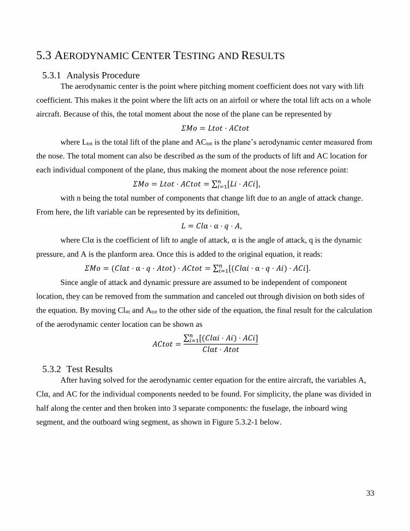
segment, and the outboard wing segment, as shown in Figure 5.3.2-1 below.
34
Figure 5-2 AC Planform without tail
For each of the segments’ areas, an approximated drawing of the plane’s planform (similar to the
one shown in Figure 5.3.2-1) was created in order to determine the areas graphically. Along with the
segment areas, the aerodynamic center locations could also be determined with a planform drawing by
finding the approximate Mean Aerodynamic Chord (MAC) location along the span of each segment and
then measuring the quarter chord distance along the MAC. This was accomplished by first measuring
the length of the tip and root chords on the plane and then drawing them to scale. The length of the root
chord was added once to each end of the tip chord and vise-versa. By connecting the diagonals of the
newly extended ends, the location of the mean aerodynamic chord (MAC) could be found by
pinpointing the intersection between the two diagonals. Since the AC is assumed to be located at a
quarter of the MAC length for subsonic aircraft, the aerodynamic centers for the first two segments were
able to be found by adding the vertical distance from the nose to the wing tip at the MAC to the quarter
chord of the MAC. For the outboard wing, it was found that the MAC was located at the midpoint of the
segment (in the spanwise direction) since the root and tip chords were equal to each other. By adding the
vertical distance from the nose, the AC for the third segment was found.
35
Once the individual areas and AC locations were found, the Cl⍺ for each component was solved
for. For most straight wings and airfoils, the Cl⍺ can be approximated as 2𝜋, however for the swept
segments of the plane, the Cl⍺ had to be found by multiplying the cosine of the sweep angle by 2𝜋.This
applied to the inboard and outboard wing segments, while the fuselage was merely approximated at 2𝜋.
Lastly, the Total area and the total aircraft Cl⍺t had to be found. The total area was determined by
adding up the individual areas and then multiplying by two since the model was split in half. The Cl⍺t
could not be calculated graphically or by assuming a value of 2𝜋. It needed to be found through testing
and analysis. For this, the aerodynamic performance program AVL was used in order to find the value
for Cl⍺t. Given all of the values, the AC could then be found by plugging everything in and multiplying
by 2 in order to account for both halves of the plane.
When the tail was considered, a fourth component had to be added to the aerodynamic center
equation that took into account the tail distance, area, and shape. First, a standard rectangular shaped tail
was selected that had a span of about 5.53 inches and a chord length of 4 inches. Being rectangular and
centered about the central axis of the plane, the Cl⍺ was assumed to be 2𝜋, the MAC was determined to
be directly in the middle of the span, and the aerodynamic center was assumed to be at the ¼ chord. The
actual AC distance from the nose of the plane was not yet decided, so several distances were tested,
ranging from 2 inches from the trailing edge of the plane to well over a foot away. Results for AC
location vs Tail were compiled and graphed along with current CG vs tail data to show tail distances that
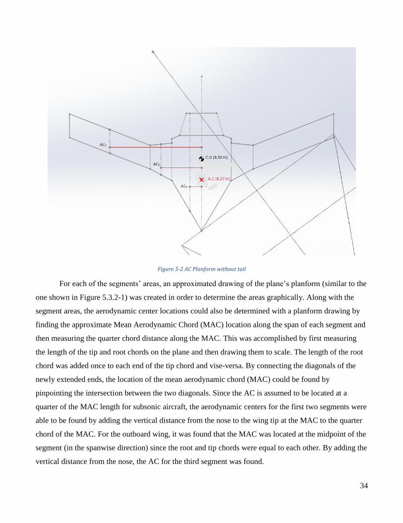
would produce stable results, as shown in Figure 5.3.2-2 below.
36
Figure 5-3 AC and CG location vs. tail Longitudinal Location
5.4 CENTER OF GRAVITY TESTING Knowing that the model experienced pitch unstable flight(static divergence) in the wind tunnel in
last year’s wind tunnel tests, the location of the center of gravity needed to be determined. This test for
the center of gravity allowed for a rough estimate for the C.G. location.
5.4.1 Test Procedures Due to the lack of equipment at the time, a makeshift C.G. locator was created using a plastic
soda bottle with curved cap. The curved top of the cap allowed the model to be balanced on a semi-fine
point.
To mark the location of the center of gravity on the model, hash marks were drawn onto the
fuselage of the model with each hash mark representing 1/4th of an inch. The zero marker was recorded
with a piece of tape on the nose.
The initial center of gravity without the attachment of the nose weight came out to be 9.5 inches
0
2
4
6
8
10
12
0 10 20 30 40
Lo
cati
on
Fro
m N
ose
(in
)
Tail Distance (in)
AC Location and CG Location vs. Tail Distance
AC Location
CG Location
37
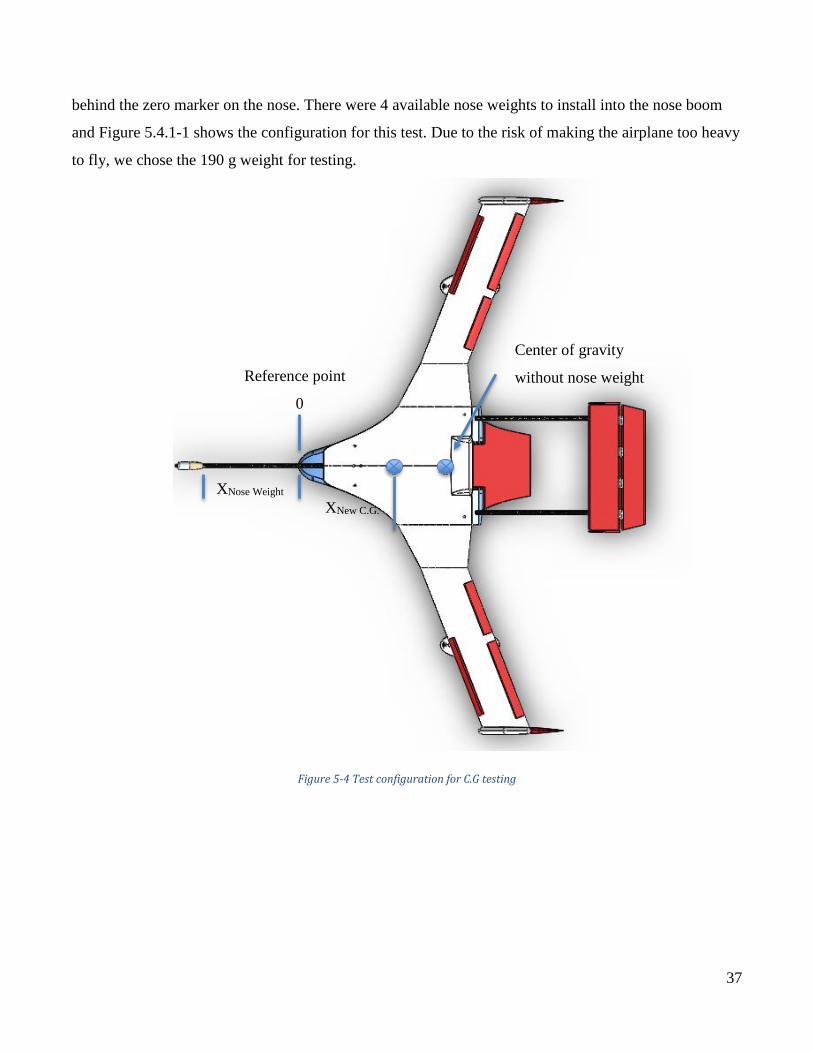
behind the zero marker on the nose. There were 4 available nose weights to install into the nose boom
and Figure 5.4.1-1 shows the configuration for this test. Due to the risk of making the airplane too heavy
to fly, we chose the 190 g weight for testing.
Figure 5-4 Test configuration for C.G testing
XNose Weight
Reference point
0
XNew C.G.
Center of gravity
without nose weight
38
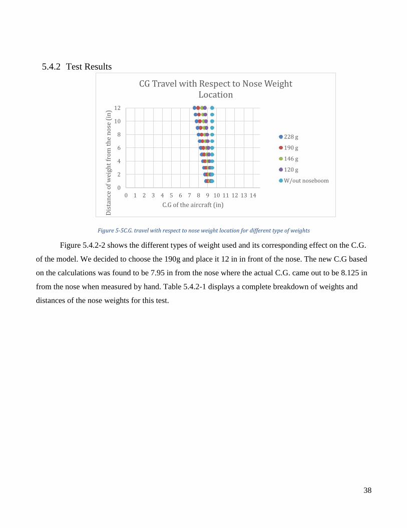
5.4.2 Test Results
Figure 5-5C.G. travel with respect to nose weight location for different type of weights
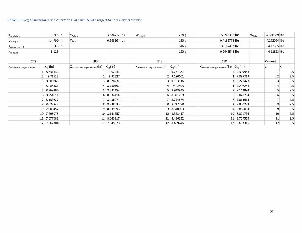
Figure 5.4.2-2 shows the different types of weight used and its corresponding effect on the C.G.
of the model. We decided to choose the 190g and place it 12 in in front of the nose. The new C.G based
on the calculations was found to be 7.95 in from the nose where the actual C.G. came out to be 8.125 in
from the nose when measured by hand. Table 5.4.2-1 displays a complete breakdown of weights and
distances of the nose weights for this test.
0
2
4
6
8
10
12
0 1 2 3 4 5 6 7 8 9 10 11 12 13 14
Dis
tan
ce o
f w
eigh
t fr
om
th
e n
ose
(in
)
C.G of the aircraft (in)
CG Travel with Respect to Nose Weight Location
228 g
190 g
146 g
120 g
W/out noseboom
39
Xcg of plane 9.5 in Wplane 3.584712 lbs Wweight 228 g 0.50265336 lbs Wtotal 4.356329 lbs
Lfuselage 14.796 in WH.T 0.268964 lbs 190 g 0.4188778 lbs 4.272554 lbs
Xdistance of H.T. 3.5 in 146 g 0.32187452 lbs 4.17555 lbs
Xcg actual 8.125 in 120 g 0.2645544 lbs 4.11823 lbs
Current
Xdistance of weight in boom (in) Xcg (in) Xdistance of weight in boom (in) Xcg (in) Xdistance of weight in boom (in) Xcg (in) Xdistance of weight in boom (in) Xcg (in) x x
1 8.831534 1 9.02431 1 9.257187 1 9.399953 1 9.5
2 8.71615 2 8.92627 2 9.180101 2 9.335713 2 9.5
3 8.600765 3 8.828231 3 9.103016 3 9.271473 3 9.5
4 8.485381 4 8.730192 4 9.02593 4 9.207233 4 9.5
5 8.369996 5 8.632153 5 8.948845 5 9.142994 5 9.5
6 8.254611 6 8.534114 6 8.871759 6 9.078754 6 9.5
7 8.139227 7 8.436074 7 8.794674 7 9.014514 7 9.5
8 8.023842 8 8.338035 8 8.717588 8 8.950274 8 9.5
9 7.908457 9 8.239996 9 8.640503 9 8.886034 9 9.5
10 7.793073 10 8.141957 10 8.563417 10 8.821794 10 9.5
11 7.677688 11 8.043917 11 8.486332 11 8.757555 11 9.5
12 7.562304 12 7.945878 12 8.409246 12 8.693315 12 9.5
228 190 146 120
Table 5-2 Weight breakdown and calculations of new C.G with respect to nose weights location
40
5.6 STATIC WING LOADING TEST AND RESULTS
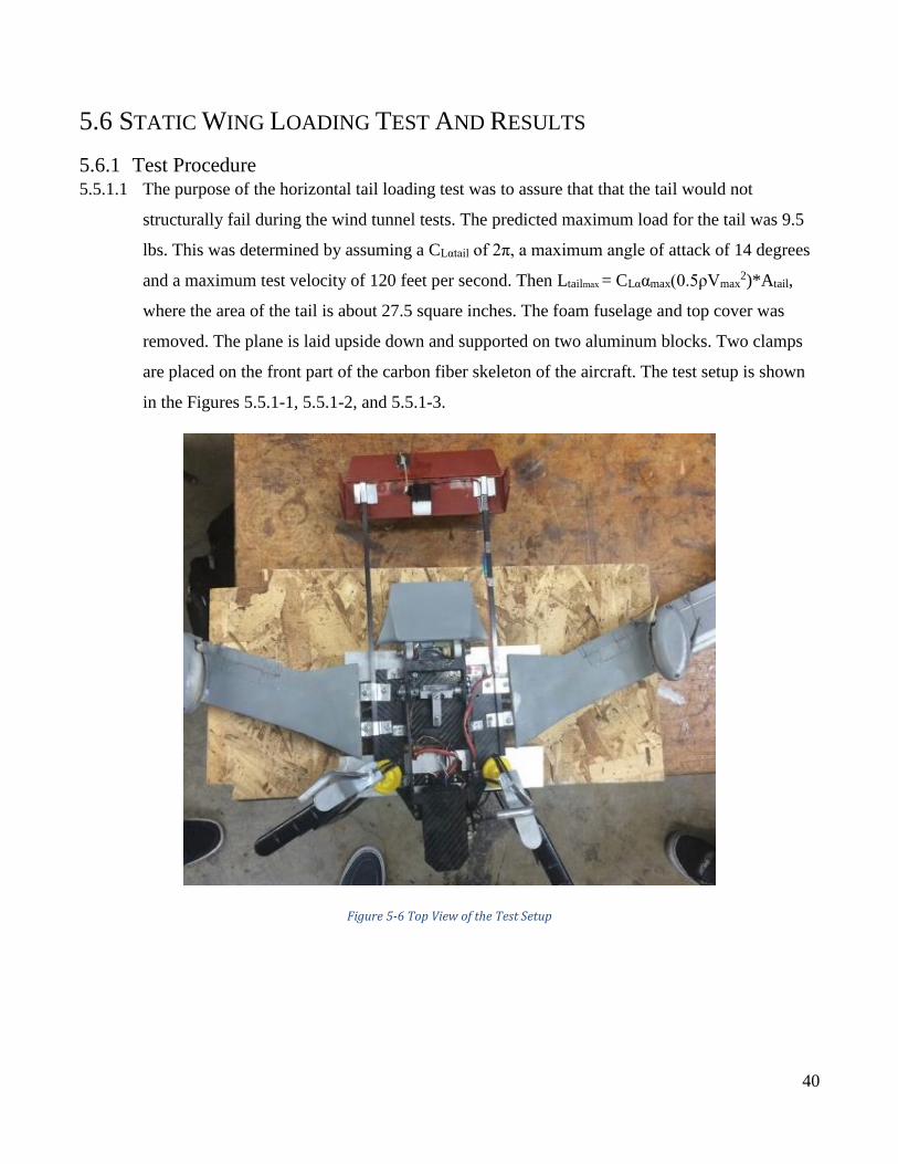
5.6.1 Test Procedure 5.5.1.1 The purpose of the horizontal tail loading test was to assure that that the tail would not
structurally fail during the wind tunnel tests. The predicted maximum load for the tail was 9.5
lbs. This was determined by assuming a CLαtail of 2π, a maximum angle of attack of 14 degrees
and a maximum test velocity of 120 feet per second. Then Ltailmax = CLααmax(0.5ρVmax2)*Atail,
where the area of the tail is about 27.5 square inches. The foam fuselage and top cover was
removed. The plane is laid upside down and supported on two aluminum blocks. Two clamps
are placed on the front part of the carbon fiber skeleton of the aircraft. The test setup is shown
in the Figures 5.5.1-1, 5.5.1-2, and 5.5.1-3.
Figure 5-6 Top View of the Test Setup
41
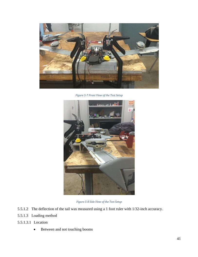
Figure 5-7 Front View of the Test Setup
Figure 5-8 Side View of the Test Setup
5.5.1.2 The deflection of the tail was measured using a 1 foot ruler with 1/32-inch accuracy.
5.5.1.3 Loading method
5.5.1.3.1 Location
Between and not touching booms
42
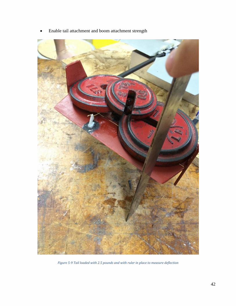
Enable tail attachment and boom attachment strength
Figure 5-9 Tail loaded with 2.5 pounds and with ruler in place to measure deflection
43
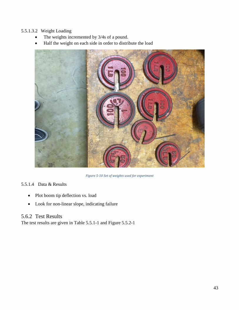
5.5.1.3.2 Weight Loading
The weights incremented by 3/4s of a pound.
Half the weight on each side in order to distribute the load
Figure 5-10 Set of weights used for experiment
5.5.1.4 Data & Results
Plot boom tip deflection vs. load
Look for non-linear slope, indicating failure
5.6.2 Test Results The test results are given in Table 5.5.1-1 and Figure 5.5.2-1
44
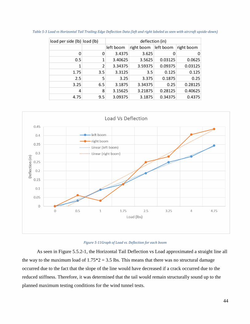
Table 5-3 Load vs Horizontal Tail Trailing Edge Deflection Data (left and right labeled as seen with aircraft upside-down)
Figure 5-11Graph of Load vs. Deflection for each boom
As seen in Figure 5.5.2-1, the Horizontal Tail Deflection vs Load approximated a straight line all
the way to the maximum load of 1.75*2 = 3.5 lbs. This means that there was no structural damage
occurred due to the fact that the slope of the line would have decreased if a crack occurred due to the
reduced stiffness. Therefore, it was determined that the tail would remain structurally sound up to the
planned maximum testing conditions for the wind tunnel tests.
load per side (lb) load (lb)
left boom right boom left boom right boom
0 0 3.4375 3.625 0 0
0.5 1 3.40625 3.5625 0.03125 0.0625
1 2 3.34375 3.59375 0.09375 0.03125
1.75 3.5 3.3125 3.5 0.125 0.125
2.5 5 3.25 3.375 0.1875 0.25
3.25 6.5 3.1875 3.34375 0.25 0.28125
4 8 3.15625 3.21875 0.28125 0.40625
4.75 9.5 3.09375 3.1875 0.34375 0.4375
deflection (in)
45
6.0 THEORY PREDICTIONS USING ATHENA VORTEX
LATTICE (AVL)
6.1 THEORY PREDICTIONS OF MODELS AERODYNAMIC CENTER VS.
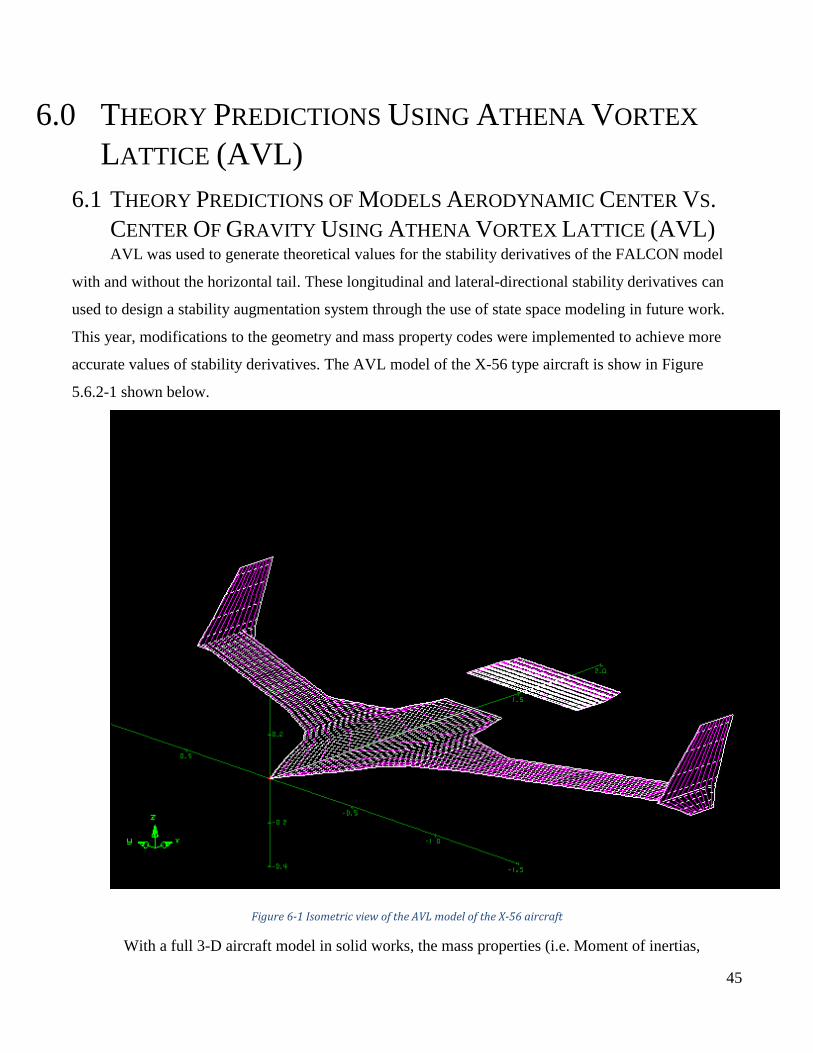
CENTER OF GRAVITY USING ATHENA VORTEX LATTICE (AVL) AVL was used to generate theoretical values for the stability derivatives of the FALCON model
with and without the horizontal tail. These longitudinal and lateral-directional stability derivatives can
used to design a stability augmentation system through the use of state space modeling in future work.
This year, modifications to the geometry and mass property codes were implemented to achieve more
accurate values of stability derivatives. The AVL model of the X-56 type aircraft is show in Figure
5.6.2-1 shown below.
Figure 6-1 Isometric view of the AVL model of the X-56 aircraft
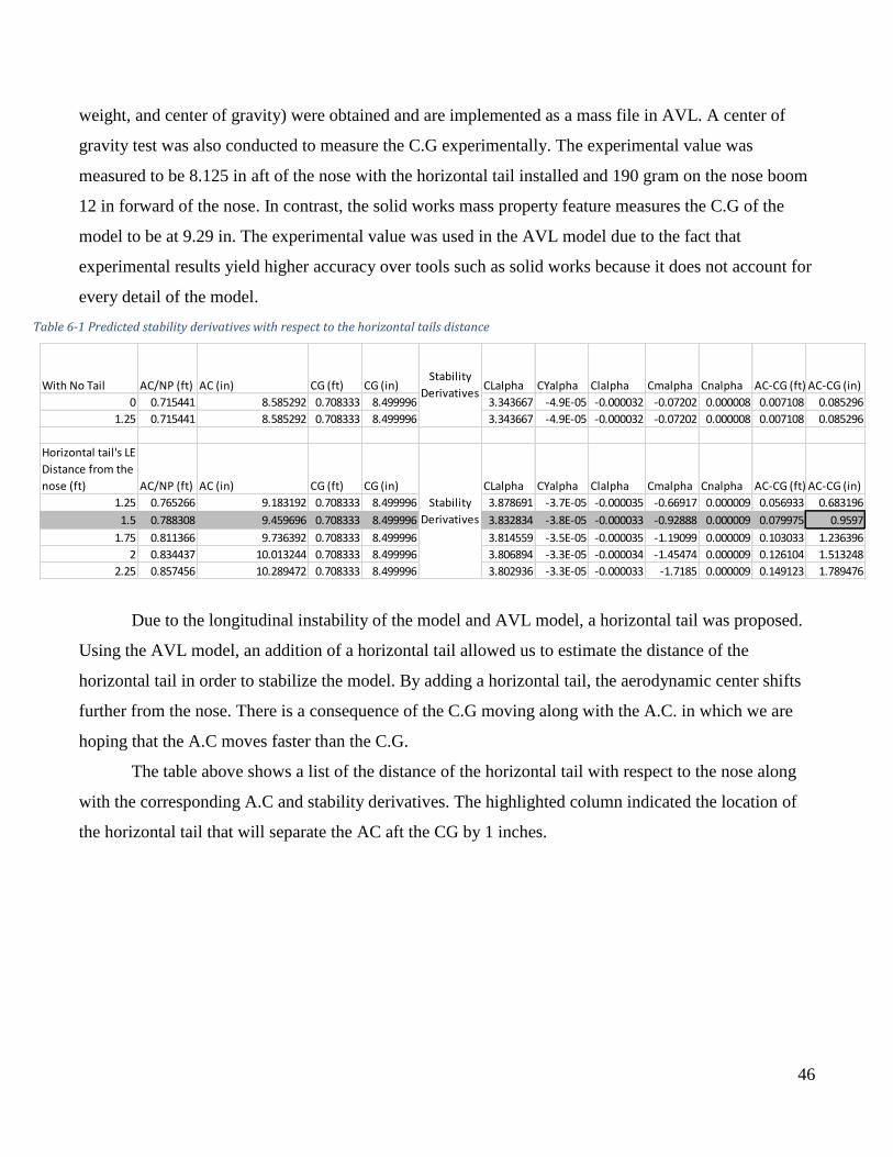
With a full 3-D aircraft model in solid works, the mass properties (i.e. Moment of inertias,
46
weight, and center of gravity) were obtained and are implemented as a mass file in AVL. A center of
gravity test was also conducted to measure the C.G experimentally. The experimental value was
measured to be 8.125 in aft of the nose with the horizontal tail installed and 190 gram on the nose boom
12 in forward of the nose. In contrast, the solid works mass property feature measures the C.G of the
model to be at 9.29 in. The experimental value was used in the AVL model due to the fact that
experimental results yield higher accuracy over tools such as solid works because it does not account for
every detail of the model.
Due to the longitudinal instability of the model and AVL model, a horizontal tail was proposed.
Using the AVL model, an addition of a horizontal tail allowed us to estimate the distance of the
horizontal tail in order to stabilize the model. By adding a horizontal tail, the aerodynamic center shifts
further from the nose. There is a consequence of the C.G moving along with the A.C. in which we are
hoping that the A.C moves faster than the C.G.
The table above shows a list of the distance of the horizontal tail with respect to the nose along
with the corresponding A.C and stability derivatives. The highlighted column indicated the location of
the horizontal tail that will separate the AC aft the CG by 1 inches.
With No Tail AC/NP (ft) AC (in) CG (ft) CG (in) CLalpha CYalpha Clalpha Cmalpha Cnalpha AC-CG (ft) AC-CG (in)
0 0.715441 8.585292 0.708333 8.499996 3.343667 -4.9E-05 -0.000032 -0.07202 0.000008 0.007108 0.085296
1.25 0.715441 8.585292 0.708333 8.499996 3.343667 -4.9E-05 -0.000032 -0.07202 0.000008 0.007108 0.085296
Horizontal tail's LE
Distance from the
nose (ft) AC/NP (ft) AC (in) CG (ft) CG (in) CLalpha CYalpha Clalpha Cmalpha Cnalpha AC-CG (ft) AC-CG (in)
1.25 0.765266 9.183192 0.708333 8.499996 3.878691 -3.7E-05 -0.000035 -0.66917 0.000009 0.056933 0.683196
1.5 0.788308 9.459696 0.708333 8.499996 3.832834 -3.8E-05 -0.000033 -0.92888 0.000009 0.079975 0.9597
1.75 0.811366 9.736392 0.708333 8.499996 3.814559 -3.5E-05 -0.000035 -1.19099 0.000009 0.103033 1.236396
2 0.834437 10.013244 0.708333 8.499996 3.806894 -3.3E-05 -0.000034 -1.45474 0.000009 0.126104 1.513248
2.25 0.857456 10.289472 0.708333 8.499996 3.802936 -3.3E-05 -0.000033 -1.7185 0.000009 0.149123 1.789476
Stability
Derivatives
Stability
Derivatives
Table 6-1 Predicted stability derivatives with respect to the horizontal tails distance
47
6.3 THEORY PREDICTIONS OF MODEL STABILITY DERIVATIVES USING
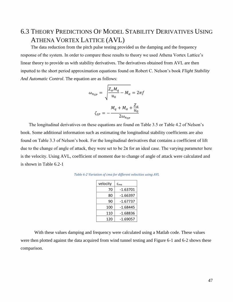
ATHENA VORTEX LATTICE (AVL) The data reduction from the pitch pulse testing provided us the damping and the frequency
response of the system. In order to compare these results to theory we used Athena Vortex Lattice’s
linear theory to provide us with stability derivatives. The derivatives obtained from AVL are then
inputted to the short period approximation equations found on Robert C. Nelson’s book Flight Stability
And Automatic Control. The equation are as follows:
𝜔𝑛𝑆𝑃= √
𝑍𝛼𝑀𝑞
𝑢0− 𝑀𝛼 = 2𝜋𝑓
𝜁𝑆𝑃 = −𝑀𝑞 + 𝑀�̇� +
𝑍𝛼
𝑢0
2𝜔𝑛𝑆𝑃
The longitudinal derivatives on these equations are found on Table 3.5 or Table 4.2 of Nelson’s
book. Some additional information such as estimating the longitudinal stability coefficients are also
found on Table 3.3 of Nelson’s book. For the longitudinal derivatives that contains a coefficient of lift
due to the change of angle of attack, they were set to be 2π for an ideal case. The varying parameter here
is the velocity. Using AVL, coefficient of moment due to change of angle of attack were calculated and
is shown in Table 6.2-1
Table 6-2 Variation of cmα for different velocities using AVL
velocity cmα
70 -1.63701
80 -1.66397
90 -1.67737
100 -1.68445
110 -1.68836
120 -1.69057
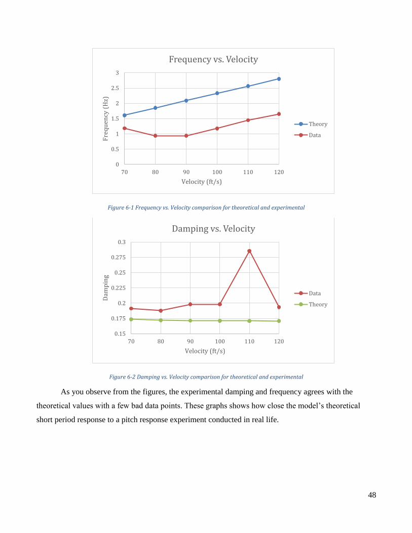
With these values damping and frequency were calculated using a Matlab code. These values
were then plotted against the data acquired from wind tunnel testing and Figure 6-1 and 6-2 shows these
comparison.
48
Figure 6-1 Frequency vs. Velocity comparison for theoretical and experimental
Figure 6-2 Damping vs. Velocity comparison for theoretical and experimental
As you observe from the figures, the experimental damping and frequency agrees with the
theoretical values with a few bad data points. These graphs shows how close the model’s theoretical
short period response to a pitch response experiment conducted in real life.
0
0.5
1
1.5
2
2.5
3
70 80 90 100 110 120
Fre
qu
ency
(H
z)
Velocity (ft/s)
Frequency vs. Velocity
Theory
Data
0.15
0.175
0.2
0.225
0.25
0.275
0.3
70 80 90 100 110 120
Dam
pin
g
Velocity (ft/s)
Damping vs. Velocity
Data
Theory
49
7.0 SIMULINK REAL-TIME CONTROL SYSTEM: (SEE
REFERENCE)
7.1 SIMULINK MODEL CONFIGURATION: (SEE REFERENCE)
7.2 THE REAL-TIME WINDOWS TARGET: (SEE REFERENCE)
7.2.1 Advantages of the Real-Time Windows Target (See Reference)
7.2.2 Known Issues with the Real-Time Windows Target (See Reference)
7.3 THE X-56 DART FLIGHT CONTROLS MODEL: (SEE REFERENCE)
7.3.1 The ArduPilot Mega(APM) Interface Subsystem (See Reference)
7.3.2 Pilot Input Subsystem (See Reference)
7.3.3 The System Status Subsystem (See Reference)
7.3.4 The Wind Tunnel Data Recorder Subsystem (See Reference)
50
8.0 WIND TUNNEL DATA ACQUISITION AND ANALYSIS
8.1 WIND TUNNEL TEST DATA ACQUISITION (SEE REFERENCE)
8.2 WIND TEST DATA ANALYSIS METHOD (SEE REFERENCE)
8.2.1 Longitudinal Stability Tests Example Calculations (See Reference)
8.2.2 Gust Response Test Example Calculations The Gust Response Analysis was use in order to find the X-56 Type natural frequency. It is done by
taking peak to peak amplitudes of the gust response data max was plotted vs. the frequency of the dual
gust vanes.
51
9.0 WIND TUNNEL TEST RESULTS
9.1 LONGITUDINAL STABILITY FREQUENCY AND PITCH DAMPING
TEST
9.1.1 Elevator Pulse Excitation Method Results The Elevator Pulse Excitation Method was to simulate a pitch doublet with the X-56 Type model
during trimmed flight within the low speed wind tunnel. The excitation test was use to create a
interference within the models flight to achieve a response. The result of the elevator pulse excitation
test was that the model was unable to reenact a pitch doublet therefore unable to acquire any feedback.
The lag time delay between the control of the joystick to the model and the speed of the servos were
unable to deliver the necessary result aim from this test.
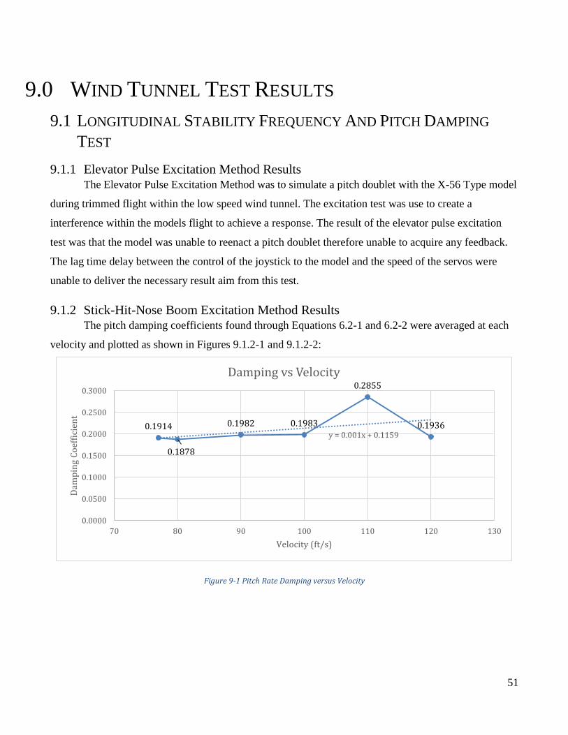
9.1.2 Stick-Hit-Nose Boom Excitation Method Results The pitch damping coefficients found through Equations 6.2-1 and 6.2-2 were averaged at each
velocity and plotted as shown in Figures 9.1.2-1 and 9.1.2-2:
Figure 9-1 Pitch Rate Damping versus Velocity
0.1914
0.1878
0.1982 0.1983
0.2855
0.1936y = 0.001x + 0.1159
0.0000
0.0500
0.1000
0.1500
0.2000
0.2500
0.3000
70 80 90 100 110 120 130
Dam
pin
g C
oef
fici
ent
Velocity (ft/s)
Damping vs Velocity
52
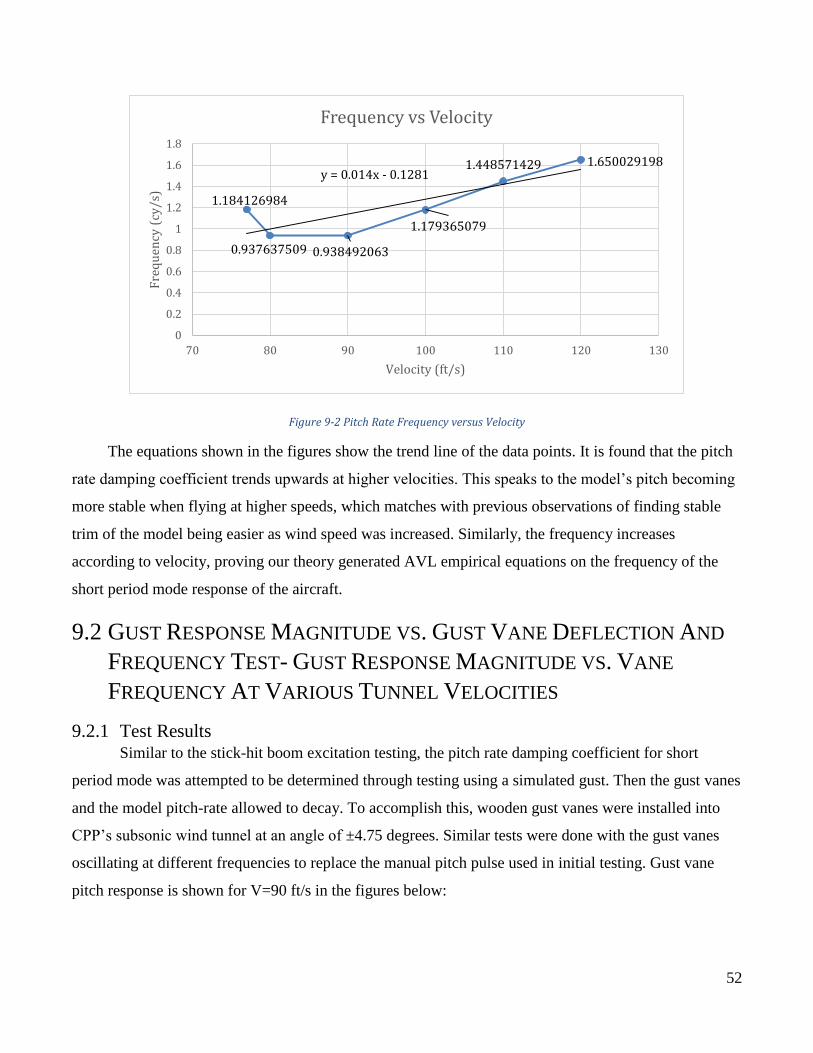
Figure 9-2 Pitch Rate Frequency versus Velocity
The equations shown in the figures show the trend line of the data points. It is found that the pitch
rate damping coefficient trends upwards at higher velocities. This speaks to the model’s pitch becoming
more stable when flying at higher speeds, which matches with previous observations of finding stable
trim of the model being easier as wind speed was increased. Similarly, the frequency increases
according to velocity, proving our theory generated AVL empirical equations on the frequency of the
short period mode response of the aircraft.
9.2 GUST RESPONSE MAGNITUDE VS. GUST VANE DEFLECTION AND
FREQUENCY TEST- GUST RESPONSE MAGNITUDE VS. VANE
FREQUENCY AT VARIOUS TUNNEL VELOCITIES
9.2.1 Test Results Similar to the stick-hit boom excitation testing, the pitch rate damping coefficient for short
period mode was attempted to be determined through testing using a simulated gust. Then the gust vanes
and the model pitch-rate allowed to decay. To accomplish this, wooden gust vanes were installed into
CPP’s subsonic wind tunnel at an angle of ±4.75 degrees. Similar tests were done with the gust vanes
oscillating at different frequencies to replace the manual pitch pulse used in initial testing. Gust vane
pitch response is shown for V=90 ft/s in the figures below:
1.184126984
0.937637509 0.938492063
1.179365079
1.448571429 1.650029198y = 0.014x - 0.1281
0
0.2
0.4
0.6
0.8
1
1.2
1.4
1.6
1.8
70 80 90 100 110 120 130
Fre
qu
ency
(cy
/s)
Velocity (ft/s)
Frequency vs Velocity
53
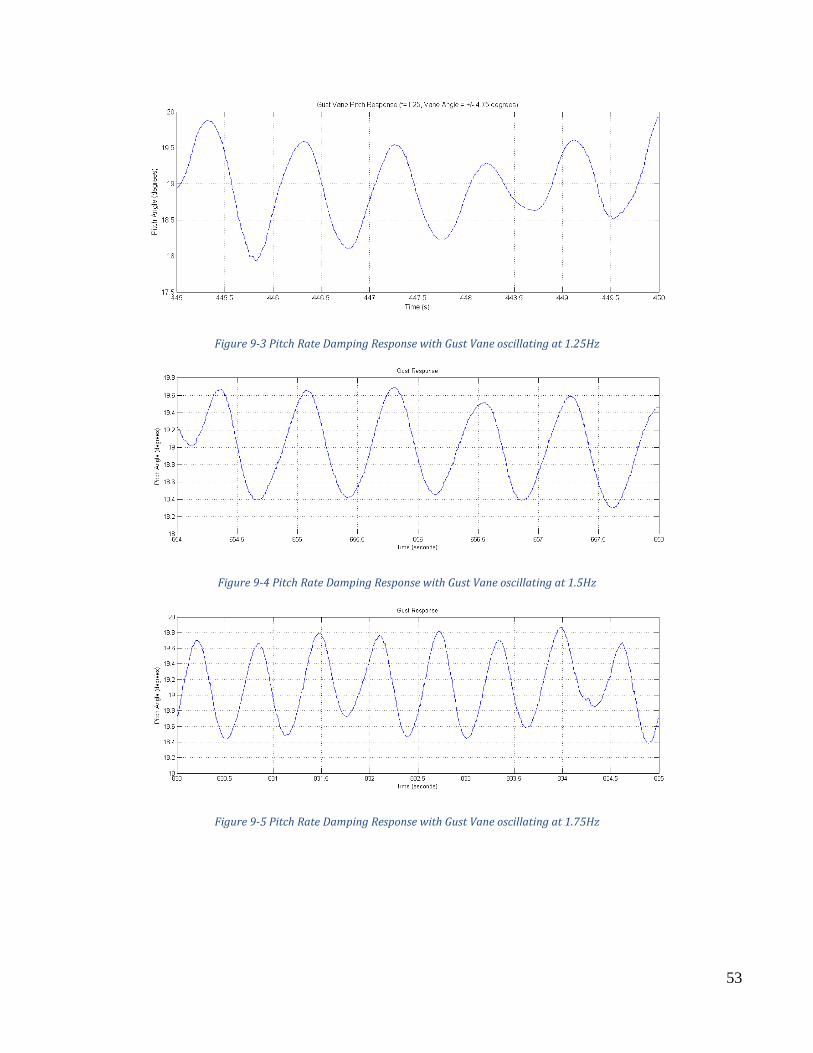
Figure 9-3 Pitch Rate Damping Response with Gust Vane oscillating at 1.25Hz
Figure 9-4 Pitch Rate Damping Response with Gust Vane oscillating at 1.5Hz
Figure 9-5 Pitch Rate Damping Response with Gust Vane oscillating at 1.75Hz
54
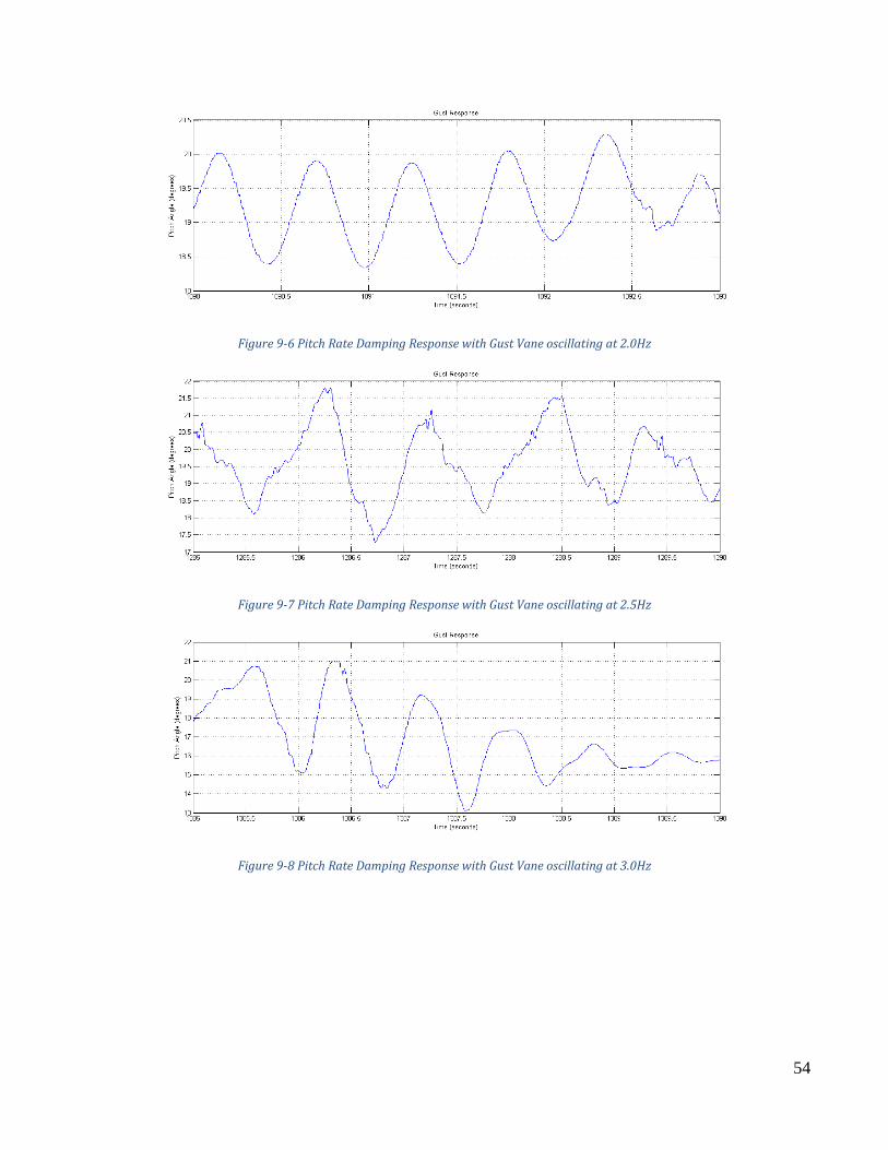
Figure 9-6 Pitch Rate Damping Response with Gust Vane oscillating at 2.0Hz
Figure 9-7 Pitch Rate Damping Response with Gust Vane oscillating at 2.5Hz
Figure 9-8 Pitch Rate Damping Response with Gust Vane oscillating at 3.0Hz
55
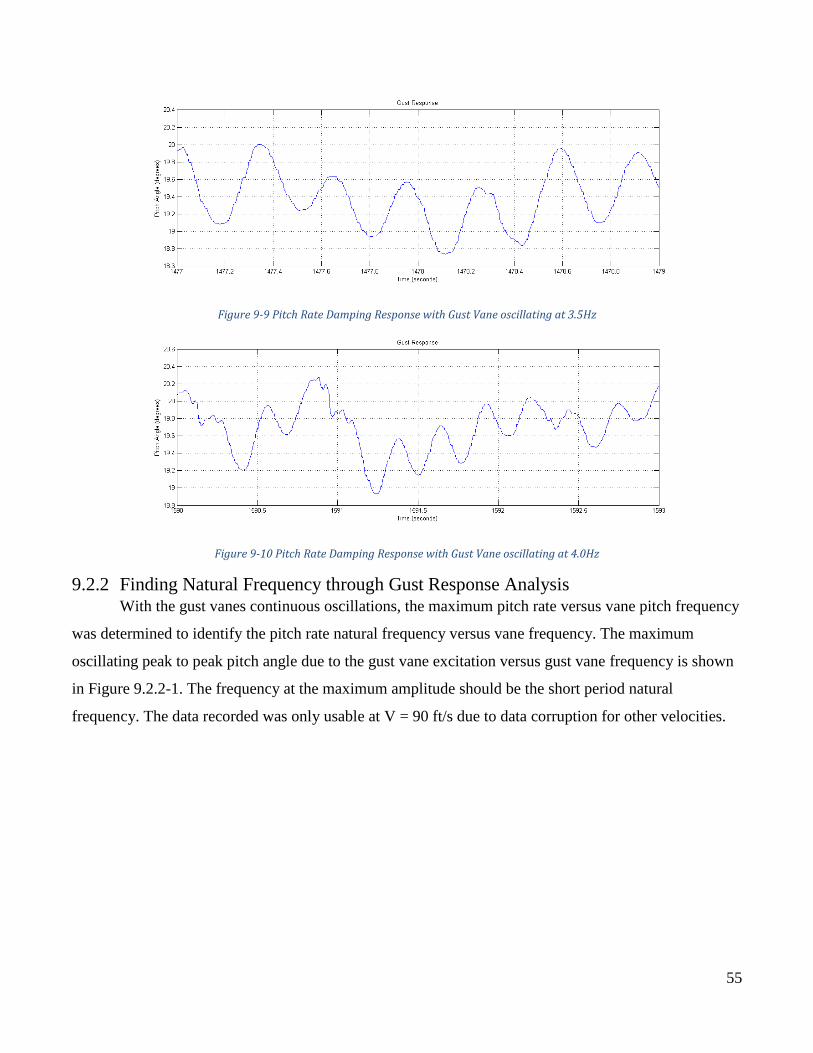
Figure 9-9 Pitch Rate Damping Response with Gust Vane oscillating at 3.5Hz
Figure 9-10 Pitch Rate Damping Response with Gust Vane oscillating at 4.0Hz
9.2.2 Finding Natural Frequency through Gust Response Analysis With the gust vanes continuous oscillations, the maximum pitch rate versus vane pitch frequency
was determined to identify the pitch rate natural frequency versus vane frequency. The maximum
oscillating peak to peak pitch angle due to the gust vane excitation versus gust vane frequency is shown
in Figure 9.2.2-1. The frequency at the maximum amplitude should be the short period natural
frequency. The data recorded was only usable at V = 90 ft/s due to data corruption for other velocities.
56
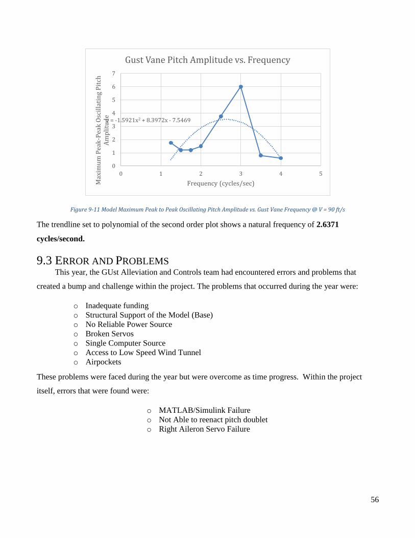
Figure 9-11 Model Maximum Peak to Peak Oscillating Pitch Amplitude vs. Gust Vane Frequency @ V = 90 ft/s
The trendline set to polynomial of the second order plot shows a natural frequency of 2.6371
cycles/second.
9.3 ERROR AND PROBLEMS This year, the GUst Alleviation and Controls team had encountered errors and problems that
created a bump and challenge within the project. The problems that occurred during the year were:
o Inadequate funding
o Structural Support of the Model (Base)
o No Reliable Power Source
o Broken Servos
o Single Computer Source
o Access to Low Speed Wind Tunnel
o Airpockets
These problems were faced during the year but were overcome as time progress. Within the project
itself, errors that were found were:
o MATLAB/Simulink Failure
o Not Able to reenact pitch doublet
o Right Aileron Servo Failure
y = -1.5921x2 + 8.3972x - 7.5469
0
1
2
3
4
5
6
7
0 1 2 3 4 5
Max
imu
m P
eak
-Pea
k O
scil
lati
ng
Pit
ch
Am
pli
tud
e
Frequency (cycles/sec)
Gust Vane Pitch Amplitude vs. Frequency
57
10.0 CONCLUSION By adding a tail and elevator to the X-56 type model mounted on a sting with a free- free flight
gimbal for pitch and plunge, trim flight was achieved in the Cal Poly Pomona Low Speed Wind Tunnel.
With trimmed flight, an elevator pulse was attempted in order to simulate a small gust disturbance to the
craft, however this gave no discernable results. The vertical excitation with an external rod hitting the
nose boom provided much clearer results and showed stable damping with short period mode, indicating
that the model was indeed capable of stable flight when disturbed or in turbulent flight conditions. The
hit- decay pitch angle and rate data was used to calculate the short period stability frequency and
damping the model. Testing the model in continuous sinusoidal gust field induced by the wind tunnel
oscillating dual gust vanes provided another way of finding the model’s natural frequency and response
magnitude in a gust environment. With all the data receive and testing, Team GUAC was able to
complete and meet various objectives that were set in the beginning of the project term. Future work that
would needed in continuing the research would be seen in Section 11.
58
11.0 RECOMMENDATION Recommendations
Below are the recommendations organized in each area of the X-56 Type Program. These
recommendations can be past down and used by future groups for the benefit of X-56 Type Program.
Structures/Fabrication
Use graphite epoxy for the tail, and elevator
Rebuild the fuselage with high density foam
Purchase a reliable power source of min 5V
Faster servo for the new tail
Replace rigid wings with flexible wings
Mass balance the flexible wings
Controls
Don’t have wires placed within the wings of the model
Color code wires
Re-label the input channels properly
Purchase a new Arduino board that has more input channels
Fix the body flap so the moment arm can be created only with the new elevator
Aerodynamics
Fix the broken servos so all the controls surfaces work on the blended wing model
Funding
Apply early for Cal Poly Grants
Look for additional sources of funding
Testing
Add Gust Alleviation Flight Control Law
Test Gust Alleviation Control Law at the same conditions of base line
59
12.0 CONTRIBUTIONS AND ACKNOWLEDGMENTS The GUst Alleviation and Controls Team (GUAC) for the X-56 Type would like take this
opportunity thank the following for the contribution and part with the project. We would like to thank
Cal Poly Pomona for the ability to use and run the Low Speed Wind Tunnel to conduct the various test
as well as the equipment used to help the project endeavors. We would also like to thank the following
people:
James Ceasari (Jim)
Dr. Ahmadi
Dr. Edberg
Amy Currier
Umbra
AIAA
Ramon (Previous Falcon member).
Brian Kelly
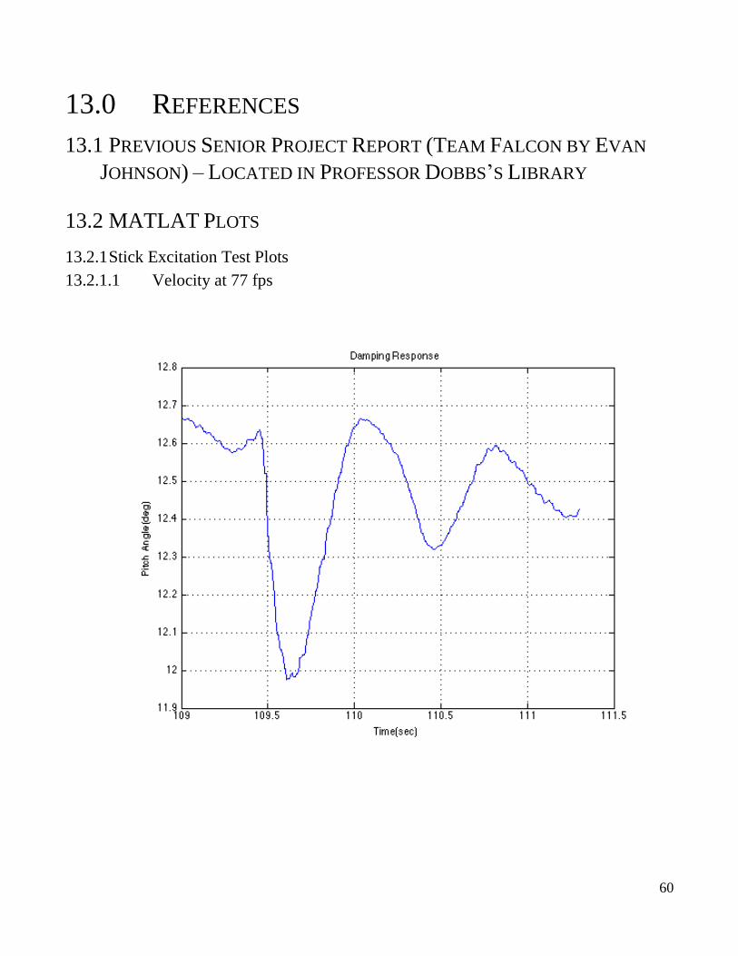
60
13.0 REFERENCES
13.1 PREVIOUS SENIOR PROJECT REPORT (TEAM FALCON BY EVAN
JOHNSON) – LOCATED IN PROFESSOR DOBBS’S LIBRARY
13.2 MATLAT PLOTS
13.2.1 Stick Excitation Test Plots
13.2.1.1 Velocity at 77 fps
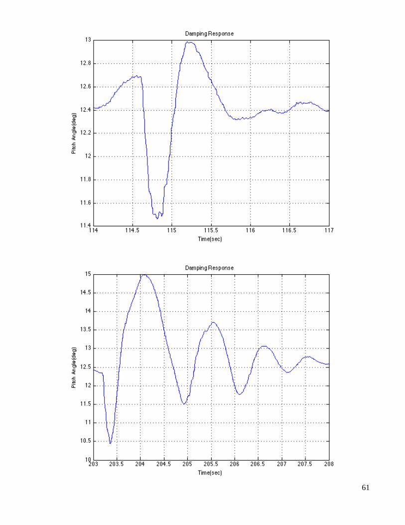
61
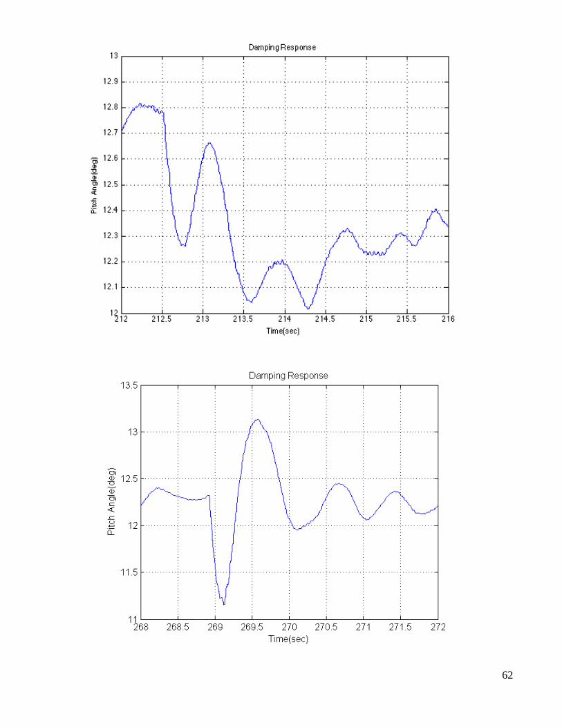
62
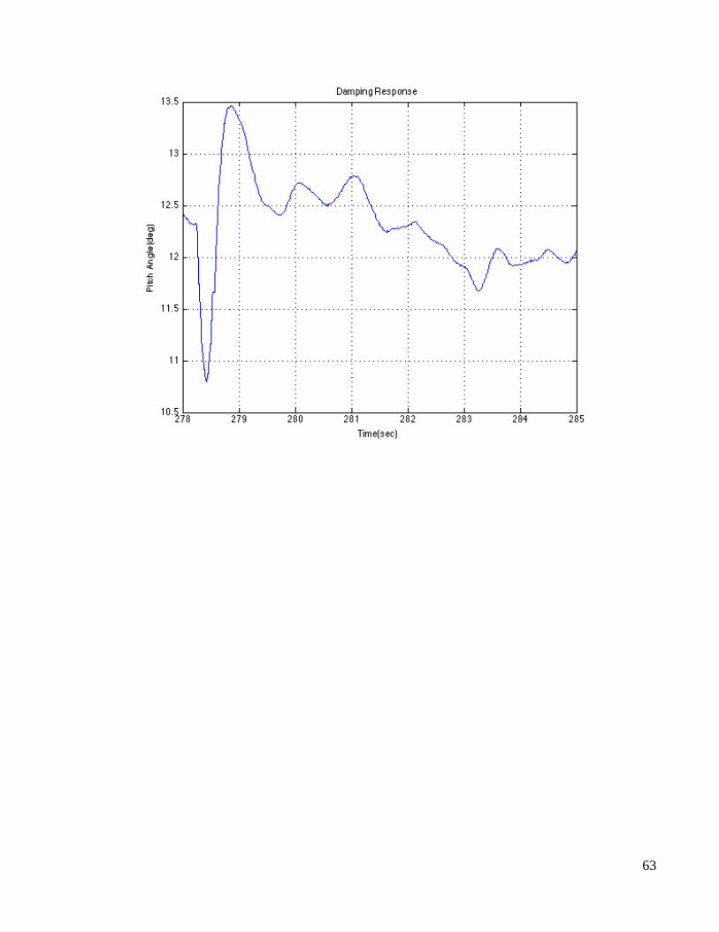
63
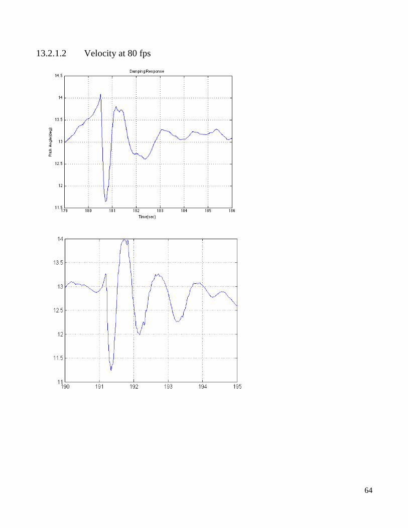
64
13.2.1.2 Velocity at 80 fps
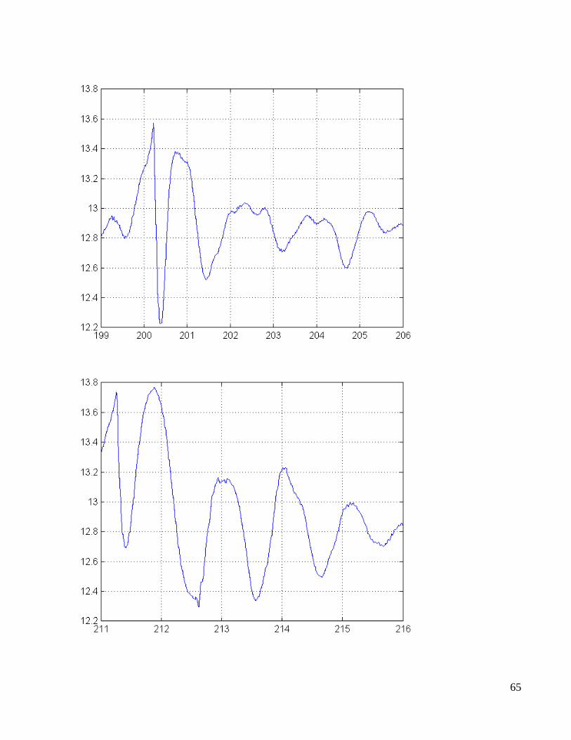
65
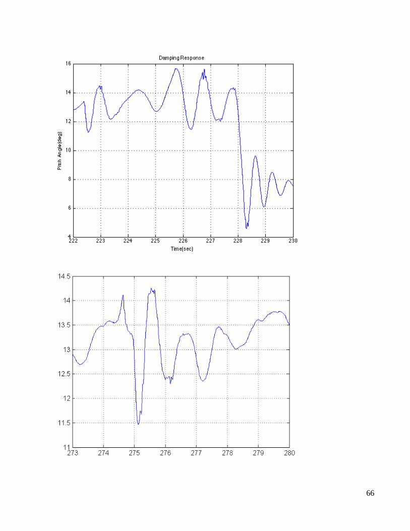
66
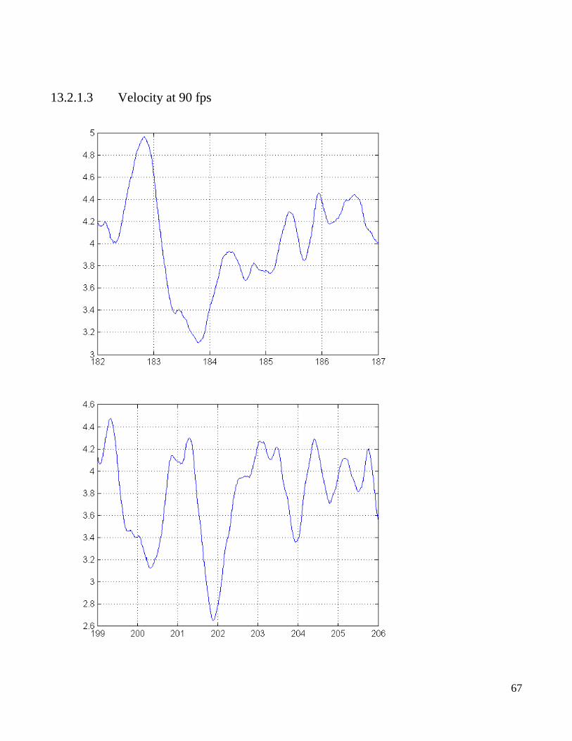
67
13.2.1.3 Velocity at 90 fps
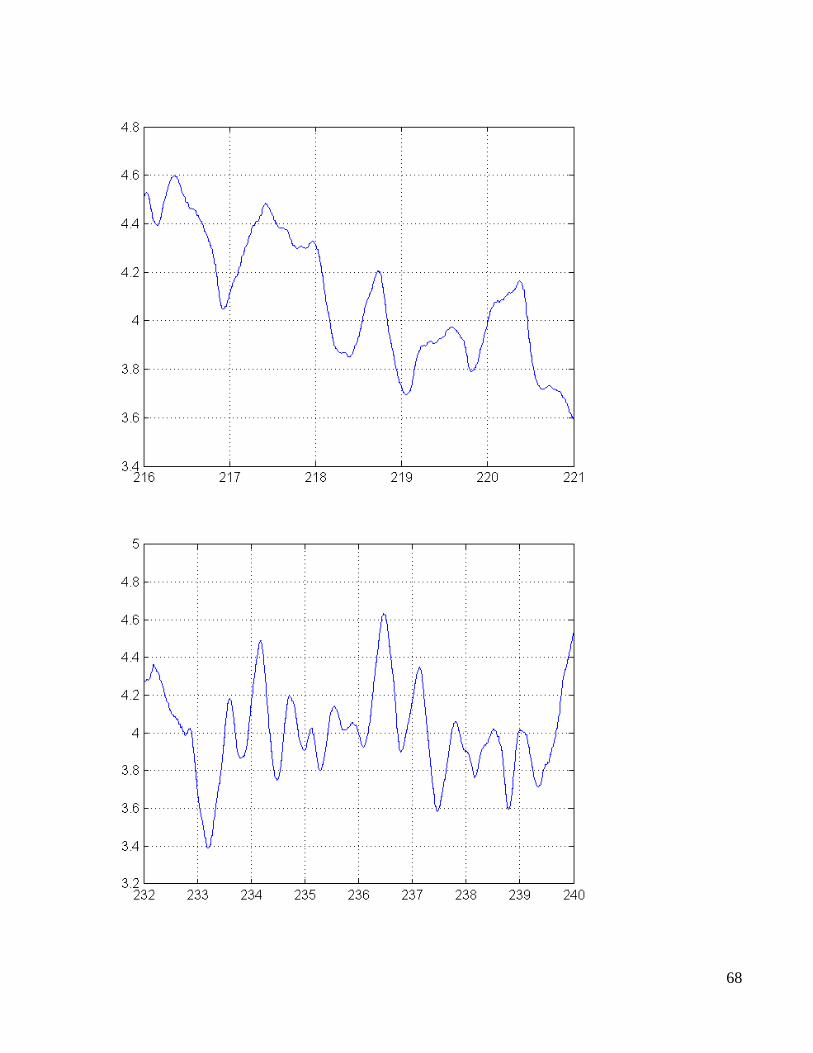
68
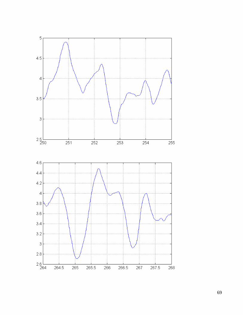
69
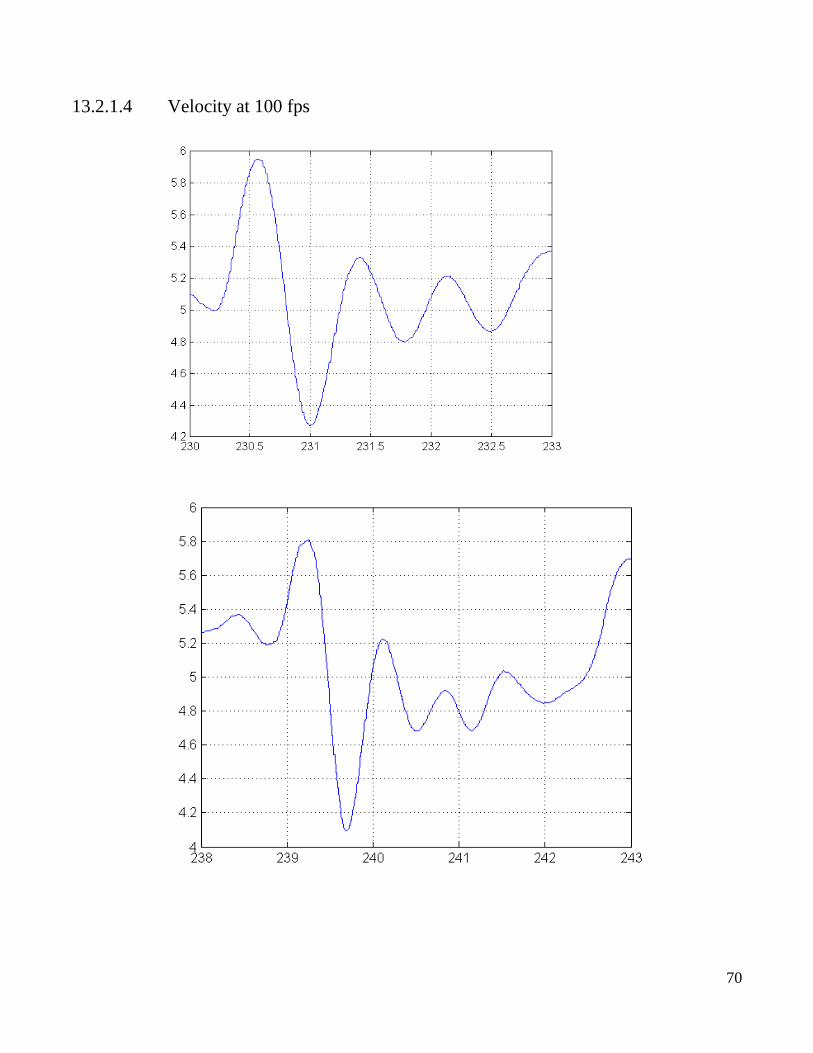
70
13.2.1.4 Velocity at 100 fps
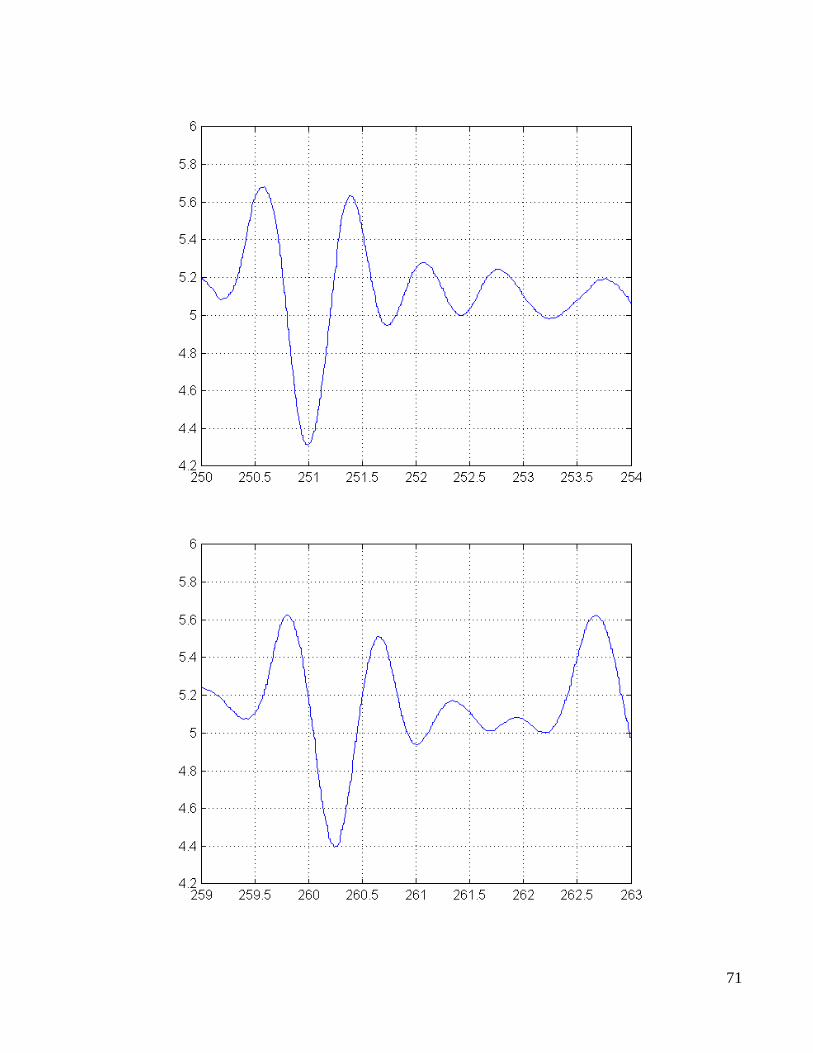
71
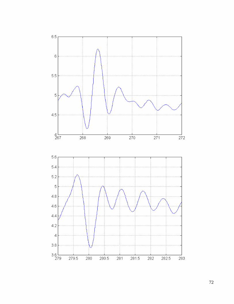
72
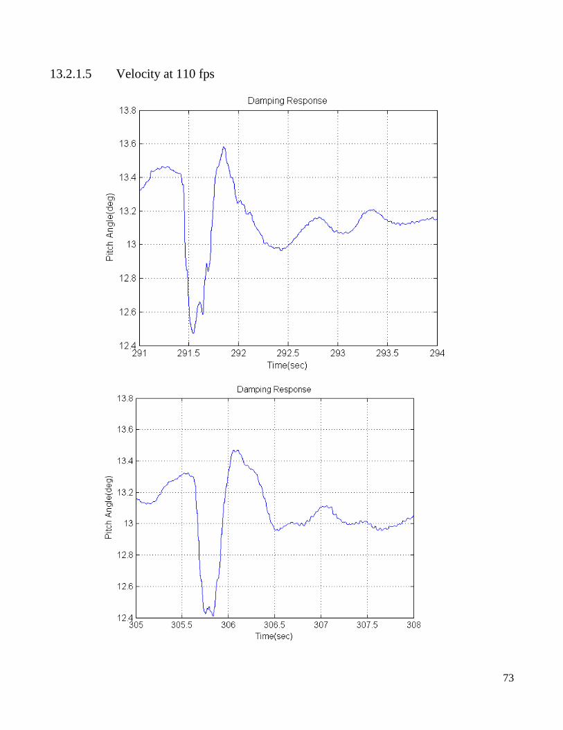
73
13.2.1.5 Velocity at 110 fps
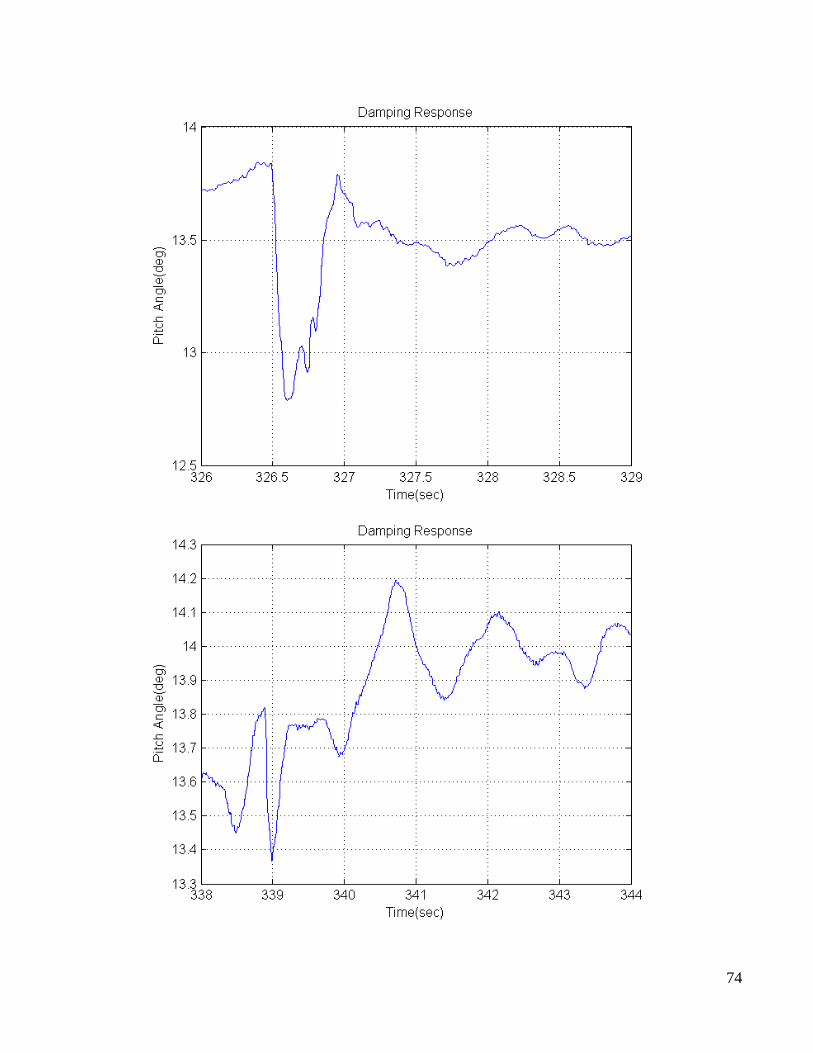
74
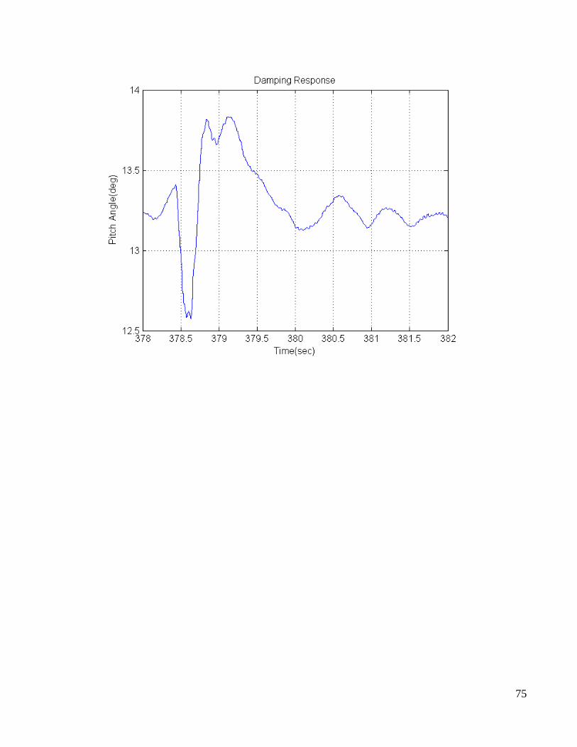
75
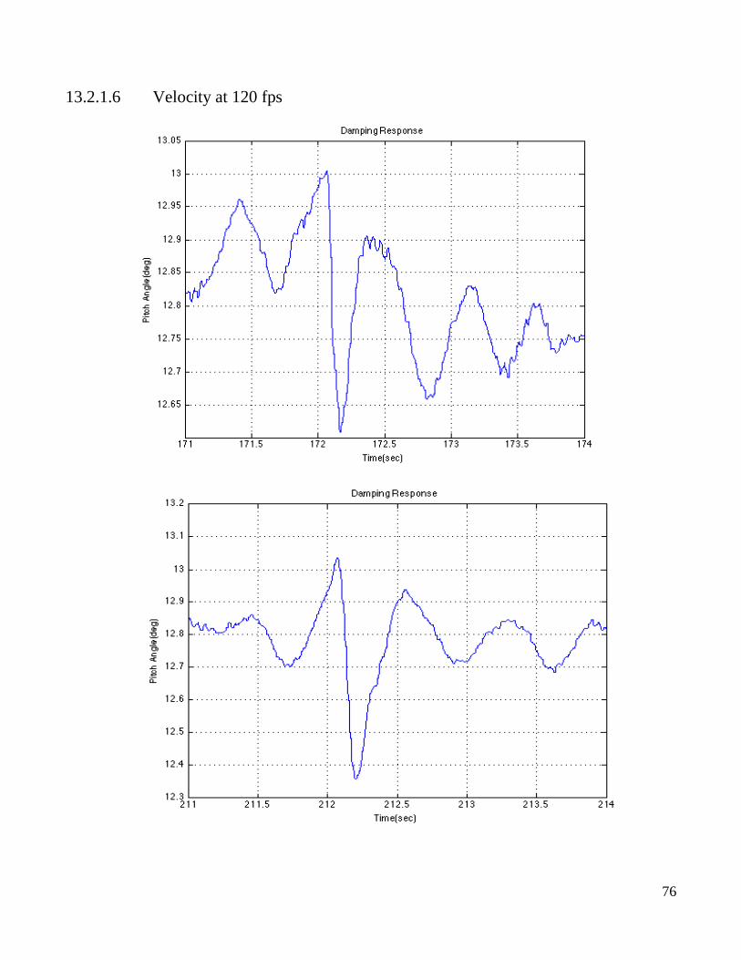
76
13.2.1.6 Velocity at 120 fps
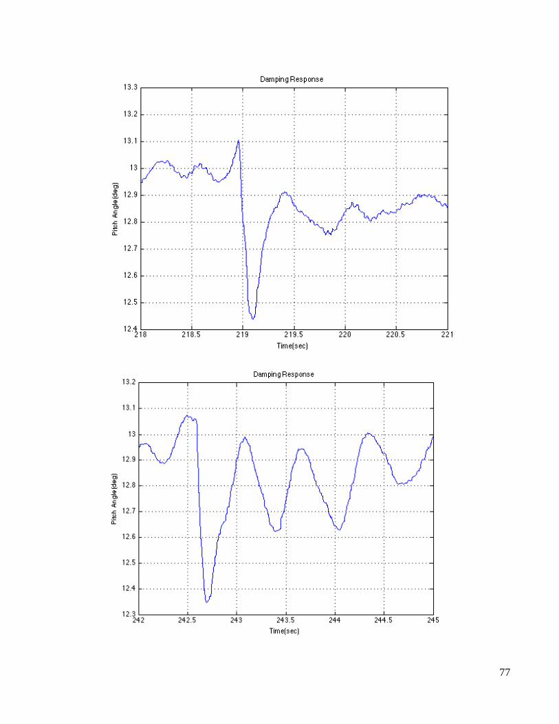
77
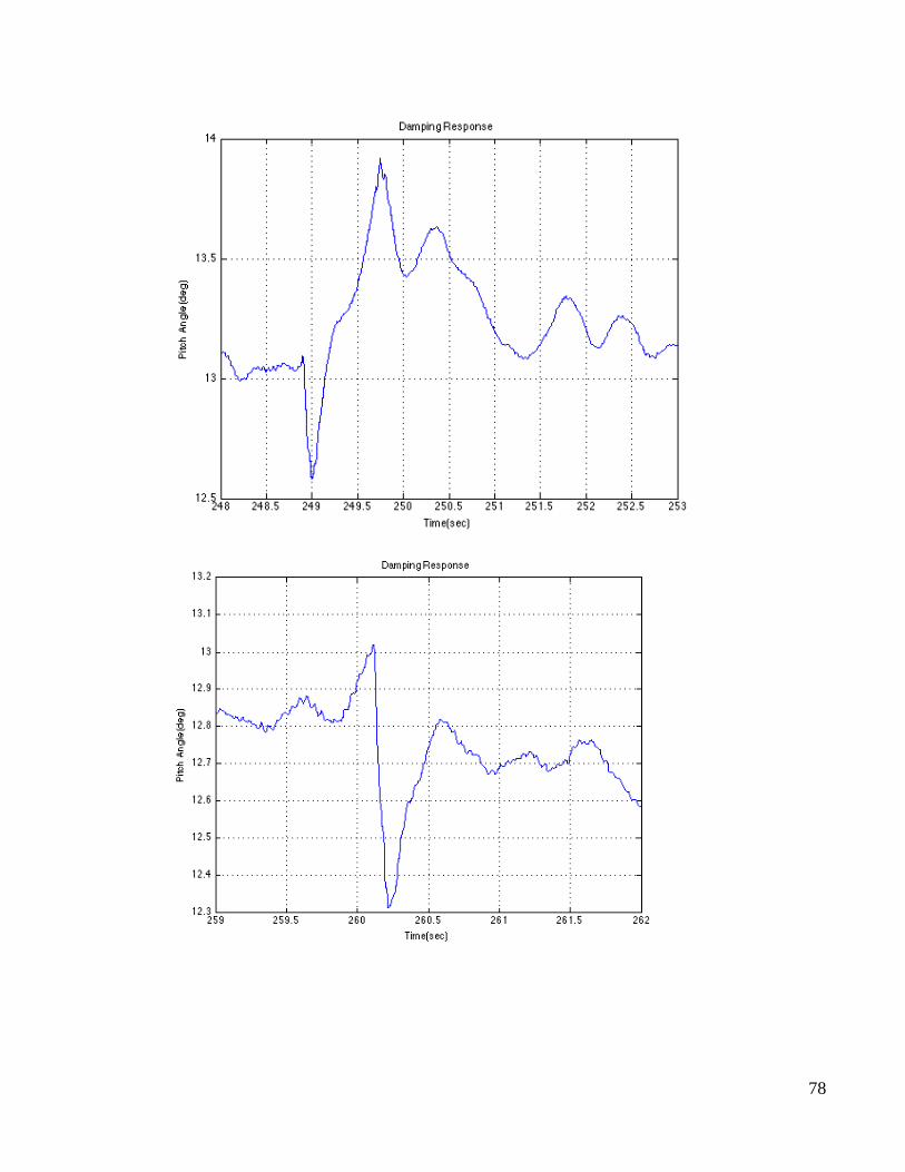
78
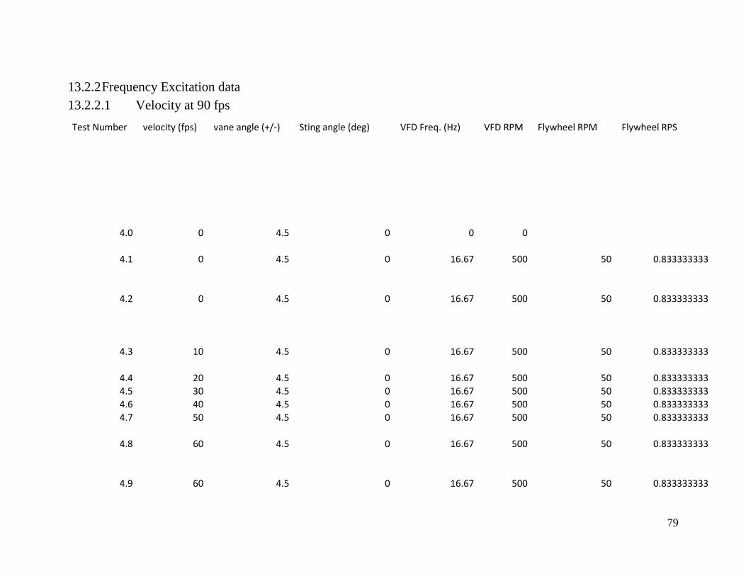
79
13.2.2 Frequency Excitation data
13.2.2.1 Velocity at 90 fps
Test Number velocity (fps) vane angle (+/-) Sting angle (deg) VFD Freq. (Hz) VFD RPM Flywheel RPM Flywheel RPS
4.0 0 4.5 0 0 0
4.1 0 4.5 0 16.67 500 50 0.833333333
4.2 0 4.5 0 16.67 500 50 0.833333333
4.3 10 4.5 0 16.67 500 50 0.833333333
4.4 20 4.5 0 16.67 500 50 0.833333333
4.5 30 4.5 0 16.67 500 50 0.833333333
4.6 40 4.5 0 16.67 500 50 0.833333333
4.7 50 4.5 0 16.67 500 50 0.833333333
4.8 60 4.5 0 16.67 500 50 0.833333333
4.9 60 4.5 0 16.67 500 50 0.833333333
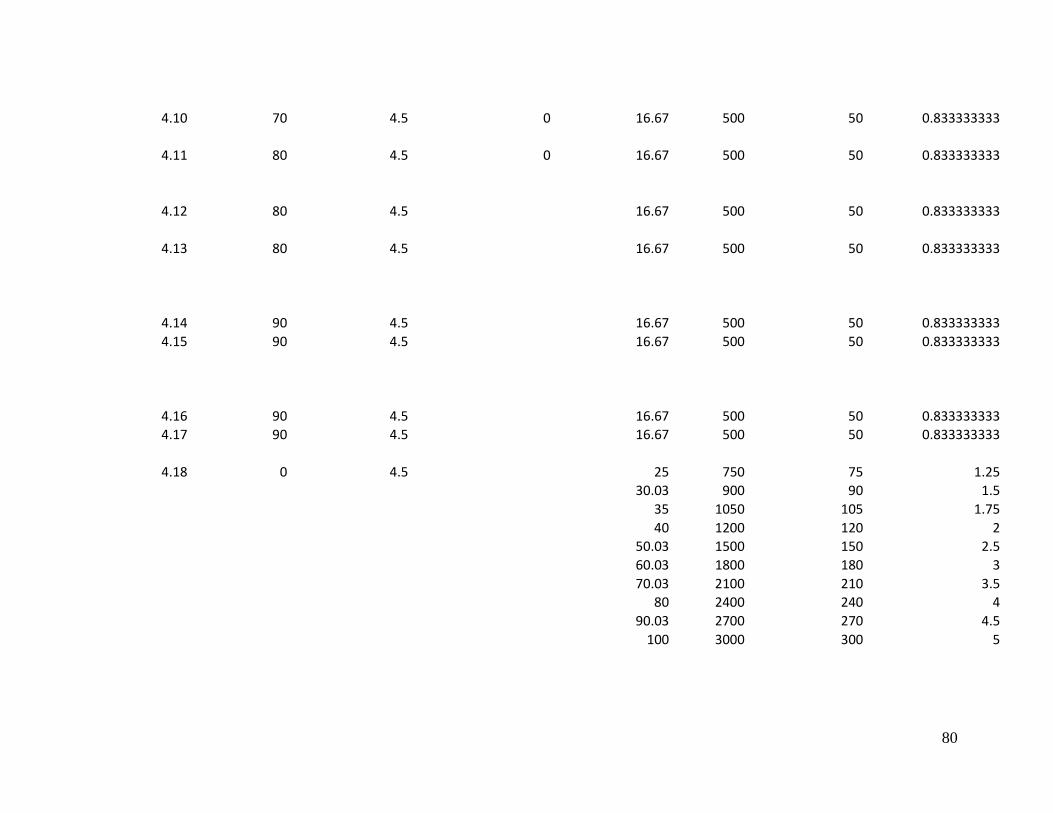
80
4.10 70 4.5 0 16.67 500 50 0.833333333
4.11 80 4.5 0 16.67 500 50 0.833333333
4.12 80 4.5
16.67 500 50 0.833333333
4.13 80 4.5
16.67 500 50 0.833333333
4.14 90 4.5
16.67 500 50 0.833333333
4.15 90 4.5
16.67 500 50 0.833333333
4.16 90 4.5
16.67 500 50 0.833333333
4.17 90 4.5
16.67 500 50 0.833333333
4.18 0 4.5
25 750 75 1.25
30.03 900 90 1.5
35 1050 105 1.75
40 1200 120 2
50.03 1500 150 2.5
60.03 1800 180 3
70.03 2100 210 3.5
80 2400 240 4
90.03 2700 270 4.5
100 3000 300 5
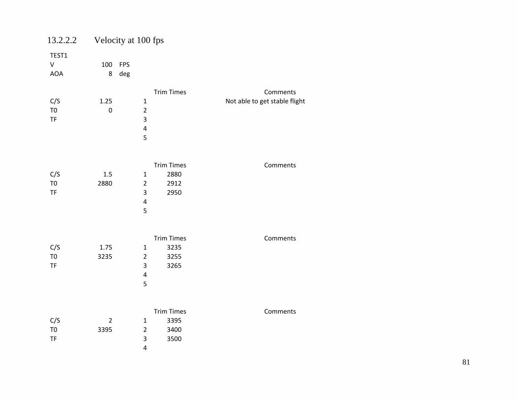
81
13.2.2.2 Velocity at 100 fps
TEST1 V 100 FPS
AOA 8 deg
Trim Times
Comments
C/S 1.25 1
Not able to get stable flight
T0 0 2 TF
3
4
5
Trim Times
Comments
C/S 1.5 1 2880 T0 2880 2 2912 TF
3 2950
4
5
Trim Times
Comments
C/S 1.75 1 3235 T0 3235 2 3255 TF
3 3265
4
5
Trim Times
Comments
C/S 2 1 3395 T0 3395 2 3400 TF
3 3500
4
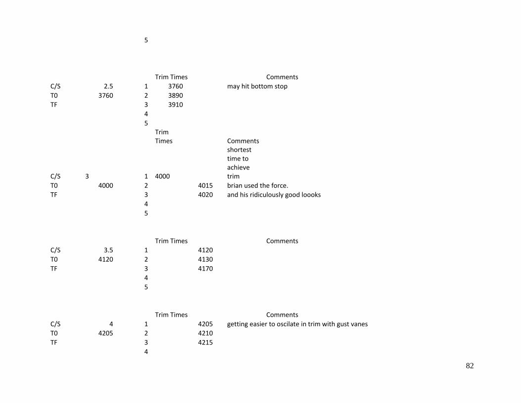
82
5
Trim Times
Comments
C/S 2.5 1 3760
may hit bottom stop T0 3760 2 3890
TF
3 3910
4
5
Trim Times
Comments
C/S 3 1 4000
shortest time to achieve trim
T0 4000 2 4015
brian used the force. TF
3 4020
and his ridiculously good loooks
4
5
Trim Times
Comments
C/S 3.5 1 4120 T0 4120 2 4130 TF
3 4170
4
5
Trim Times
Comments
C/S 4 1 4205
getting easier to oscilate in trim with gust vanes
T0 4205 2 4210 TF
3 4215
4
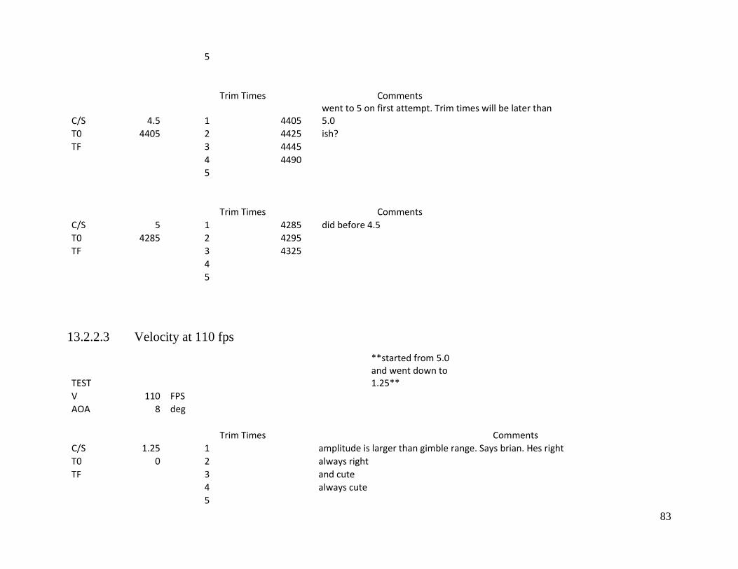
83
5
Trim Times
Comments
C/S 4.5 1 4405
went to 5 on first attempt. Trim times will be later than 5.0
T0 4405 2 4425
ish? TF
3 4445
4 4490
5
Trim Times
Comments
C/S 5 1 4285
did before 4.5 T0 4285 2 4295
TF
3 4325
4
5
13.2.2.3 Velocity at 110 fps
TEST
**started from 5.0 and went down to 1.25**
V 110 FPS AOA 8 deg
Trim Times
Comments
C/S 1.25 1
amplitude is larger than gimble range. Says brian. Hes right
T0 0 2
always right TF
3
and cute
4
always cute
5
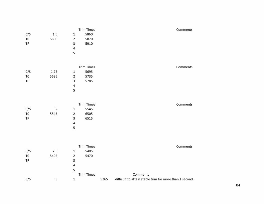
84
Trim Times
Comments
C/S 1.5 1 5860 T0 5860 2 5870 TF
3 5910
4
5
Trim Times
Comments
C/S 1.75 1 5695 T0 5695 2 5735 TF
3 5785
4
5
Trim Times
Comments
C/S 2 1 5545 T0 5545 2 6505 TF
3 6515
4
5
Trim Times
Comments
C/S 2.5 1 5405 T0 5405 2 5470 TF
3
4
5
Trim Times
Comments
C/S 3 1 5265
difficult to attain stable trim for more than 1 second.
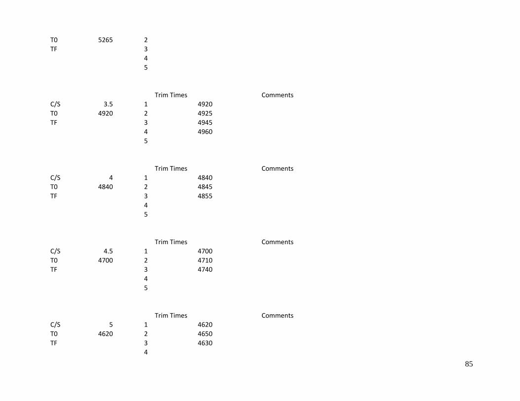
85
T0 5265 2 TF
3
4
5
Trim Times
Comments
C/S 3.5 1 4920 T0 4920 2 4925 TF
3 4945
4 4960
5
Trim Times
Comments
C/S 4 1 4840 T0 4840 2 4845 TF
3 4855
4
5
Trim Times
Comments
C/S 4.5 1 4700 T0 4700 2 4710 TF
3 4740
4
5
Trim Times
Comments
C/S 5 1 4620 T0 4620 2 4650 TF
3 4630
4
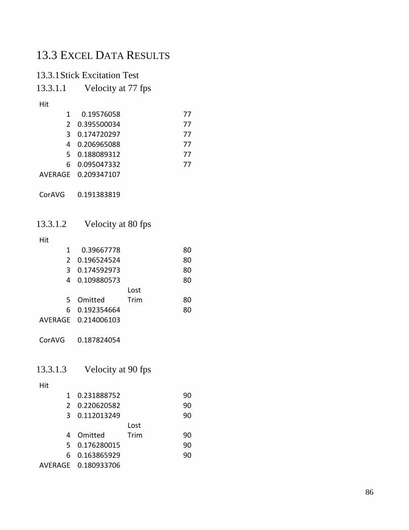
86
13.3 EXCEL DATA RESULTS
13.3.1 Stick Excitation Test
13.3.1.1 Velocity at 77 fps
Hit 1 0.19576058
77
2 0.395500034
77 3 0.174720297
77
4 0.206965088
77 5 0.188089312
77
6 0.095047332
77
AVERAGE 0.209347107
CorAVG 0.191383819
13.3.1.2 Velocity at 80 fps
Hit 1 0.39667778
80
2 0.196524524
80 3 0.174592973
80
4 0.109880573
80
5 Omitted Lost Trim 80
6 0.192354664
80 AVERAGE 0.214006103
CorAVG 0.187824054
13.3.1.3 Velocity at 90 fps
Hit 1 0.231888752
90
2 0.220620582
90 3 0.112013249
90
4 Omitted Lost Trim 90
5 0.176280015
90 6 0.163865929
90
AVERAGE 0.180933706
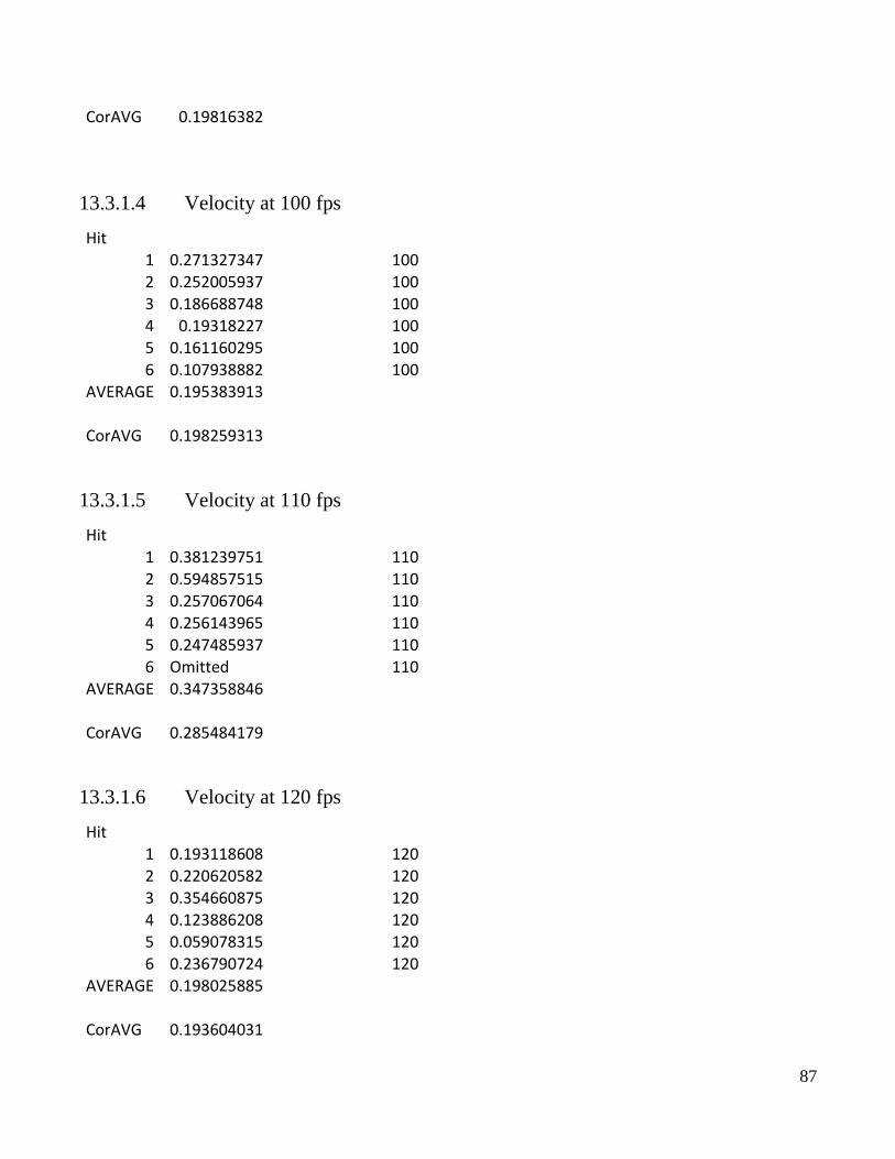
87
CorAVG 0.19816382
13.3.1.4 Velocity at 100 fps
Hit 1 0.271327347
100
2 0.252005937
100 3 0.186688748
100
4 0.19318227
100 5 0.161160295
100
6 0.107938882
100 AVERAGE 0.195383913
CorAVG 0.198259313
13.3.1.5 Velocity at 110 fps
Hit 1 0.381239751
110
2 0.594857515
110 3 0.257067064
110
4 0.256143965
110 5 0.247485937
110
6 Omitted
110 AVERAGE 0.347358846
CorAVG 0.285484179
13.3.1.6 Velocity at 120 fps
Hit 1 0.193118608
120
2 0.220620582
120 3 0.354660875
120
4 0.123886208
120 5 0.059078315
120
6 0.236790724
120 AVERAGE 0.198025885
CorAVG 0.193604031

88
13.4 BOOKS
Nelson, Robert. Flight Stability and Automatic Control. 2th
ed. McGraw-Hill Book Co 1998
13.5 OTHER DOCUMENTS
Previous Years Final Report (Located in Professor Dobb’s Library)
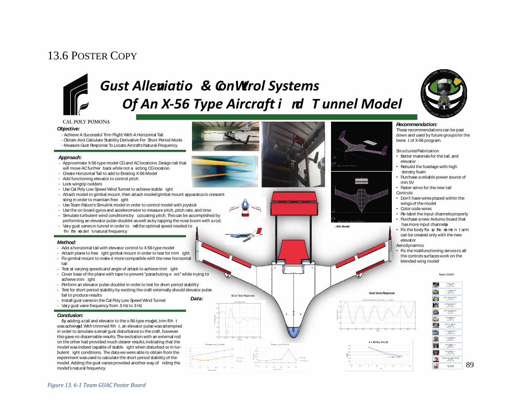
89
13.6 POSTER COPY
Gust Alleviation & Con trol Systems Of An X-56 Type Aircraft
Wi nd T unnel Model
Objective: - Achieve A Successful Trim Flight With A Horizontal Tail.
- Obtain And Calculate Stability Derivative For Short Period Mode
- Measure Gust Response To Locate Aircrafts Natural Frequency
!
! "#$"%&'( %) %$*"'!"#$%!&'%( !)*!
+, - , .!/0- !1!0230!455'%( 6 78#9: ; : %$<=5#!
+*, - ./'! "#$"%&'( %) %$*"!&> '?( 4!@$A$!
+0B3.!C- - !1!- 3, 2!5> '?( 4%$A$6 ?; $'D<7: ; !
0*%1'2#) ."#3'4/5.*&5'6) $7) **"'E =: *?=!F$?#': !+0B3.!3- C!1!2- 3G!
??9$?#': 6 78#9: ; : %$<=5#!
2#) ."#3'4/5.*&5'6) $7) **"!&: %?!)'%!HI : : !+/BC.!J /3!1!02/0!
K#8L%<*I : : 6 ?; $'D<7: ; !
0*%1'8*"#1/) %&795'6) $7) **"!M'DD!N : ?$( %!
+, - , .!, , 3!1!0J , / !> : ?$%#O6 I $( : : <7: ; !
8*"#1/) %&795'6) $7) **"!H=?'%$D5!E #'%4: !+, - , .!23, !1!2- , - !
*=?'%$D5?#'%4: 6 ?; $'D<7: ; !
0*%1'4."- 9.- "%3'6) $7) **"!"$%%=*!PD$*Q!
+GGB.!0B, !1!3, C3!477D$*Q6 78#9: ; : %$<=5#!
2: 7*;'<%="79%>#) '6) $7) **"!)$8: %!R: %?!
+G0G.!GG- !1!/G- 3!K$8: %Q: %?6 78#9: ; : %$<=5#!
2: 7*;'<7) %) 97%3'? @9*"!S*I $!N 'DD'$; 8!
+G0G.!/B- !1!- 0B, !$I *$K#%=> 'DD'$; 86 ; 8%<7: ; !
8*"#1/) %&795'4- , , #". !P*I 84$D!@#%=T!
+/BC.!GB, !1!BC3C!7*I 84$D<%#%=T3J 6 I $( : : <7: ; !
8*"#1/) %&795'4- , , #". !S%$( '!U=*%$%5=T!+303.!C, - !1!0, 2, !
$%$( '( 6 78#9: ; : %$<=5#!
! "#$"%&'%) 1'2#) ."#3'4/5.*&5'81A75#"!!VA$%!): ( %8: %!+/BC.!J 2B!1!CBCG!
=*K: ( %8: %00/6 ?; $'D<7: ; !
<%9- 3./'81A75#"!W4=A=%!&: OO8!
Method:- Add a horizontal tail with elevator control to X-56 type model
- Attach plane to free ight gimbal mount in order to test for trim ight
- Fix gimbal mount to make it more compatible with the new horizontal
tail
- Test at varying speeds and angle of attack to achieve trim ight
- Cover base of the plane with tape to prevent “parachuting e ect” while trying to
achieve trim ight
- Perform an elevator pulse-doublet in order to test for short period stability
- Test for short period stability by exciting the craft externally should elevator pulse
fail to produce results
- Install gust vanes in the Cal Poly Low Speed Wind Tunnel
- Vary gust vane frequency from .5 Hz to 3 Hz
Recommendation:These recommendations can be past
down and used by future groups for the
bene t of X-56 program.
Structures/Fabrication
• Better materials for the tail, and
elevator
• Rebuild the fuselage with high
density foam
• Purchase a reliable power source of
min 5V
• Faster servo for the new tail
Controls
• Don’t have wires placed within the
wings of the model
• Color code wires
• Re-label the input channels properly
• Purchase a new Arduino board that
has more input channels
• Fix the body fla
p
so the mo me n t arm
can be created only with the new
elevator
Aerodynamics
• Fix the malifunctioning servos to all
the controls surfaces work on the
blended wing model
Conclusion: By adding a tail and elevator to the x-56 type model, trim flig h t
was achieved. With trimmed flig h t, an elevator pulse was attempted
in order to simulate a small gust disturbance to the craft, however
this gave no discernable results. The excitation with an external rod
on the other had provided much clearer results, indicating that the
model was indeed capable of stable ight when disturbed or in tur-
bulent ight conditions. The data we were able to obtain from the
experiment was used to calculate the short period stability of the
model. Adding the gust vanes provided another way of nding the
model’s natural frequency.
Approach:- Approximate X-56 type model CG and AC locations. Design tail that
will move AC further back while not a ecting CG location.
- Create Horizontal Tail to add to Existing X-56 Model
- Add functioning elevator to control pitch
- Lock wingtip rudders
- Use Cal Poly Low Speed Wind Tunnel to achieve stable ight
- Attach model to gimbal mount, then attach model/gimbal mount apparatus to crescent
sting in order to maintain free ight
- Use Team Falcon’s Simulink model in order to control model with joystick
- Use the on board gyros and accelerometer to measure pitch, pitch rate, and time
- Simulate turbulent wind conditions by uctuating pitch. This can be accomplished by
performing an elevator pulse-doublet as well as by tapping the nose boom with a rod.
- Vary gust vanes in tunnel in order to nd the optimal speed needed to
fin
d
the mo del ’s natural frequency
Data:
- AVL Model
Gust Vane ResponseStick Test Reponse
Team GUAC-
Figure 13. 6-1 Team GUAC Poster Board
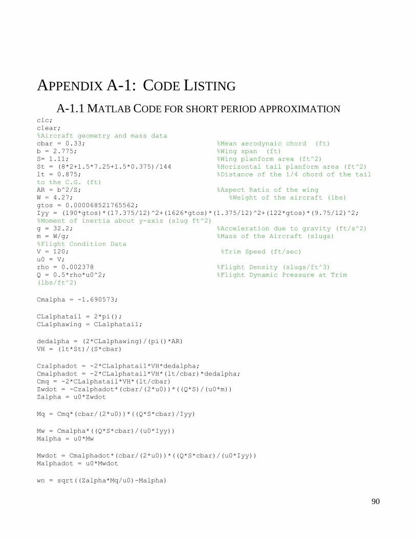
90
APPENDIX A-1: CODE LISTING
A-1.1 MATLAB CODE FOR SHORT PERIOD APPROXIMATION clc; clear; %Aircraft geometry and mass data cbar = 0.33; %Mean aerodynaic chord (ft) b = 2.775; %Wing span (ft) S= 1.11; %Wing planform area (ft^2) St = (8*2+1.5*7.25+1.5*0.375)/144 %Horizontal tail planform area (ft^2) lt = 0.875; %Distance of the 1/4 chord of the tail
to the C.G. (ft) AR = b^2/S; %Aspect Ratio of the wing W = 4.27; %Weight of the aircraft (lbs) gtos = 0.000068521765562; Iyy = (190*gtos)*(17.375/12)^2+(1626*gtos)*(1.375/12)^2+(122*gtos)*(9.75/12)^2;
%Moment of inertia about y-axis (slug ft^2) g = 32.2; %Acceleration due to gravity (ft/s^2) m = W/g; %Mass of the Aircraft (slugs) %Flight Condition Data V = 120; %Trim Speed (ft/sec) u0 = V; rho = 0.002378 %Flight Density (slugs/ft^3) Q = 0.5*rho*u0^2; %Flight Dynamic Pressure at Trim
(lbs/ft^2)
Cmalpha = -1.690573;
CLalphatail = 2*pi(); CLalphawing = CLalphatail;
dedalpha = (2*CLalphawing)/(pi()*AR) VH = (lt*St)/(S*cbar)
Czalphadot = -2*CLalphatail*VH*dedalpha; Cmalphadot = -2*CLalphatail*VH*(lt/cbar)*dedalpha; Cmq = -2*CLalphatail*VH*(lt/cbar) Zwdot = -Czalphadot*(cbar/(2*u0))*((Q*S)/(u0*m)) Zalpha = u0*Zwdot
Mq = Cmq*(cbar/(2*u0))*((Q*S*cbar)/Iyy)
Mw = Cmalpha*((Q*S*cbar)/(u0*Iyy)) Malpha = u0*Mw
Mwdot = Cmalphadot*(cbar/(2*u0))*((Q*S*cbar)/(u0*Iyy)) Malphadot = u0*Mwdot
wn = sqrt((Zalpha*Mq/u0)-Malpha)
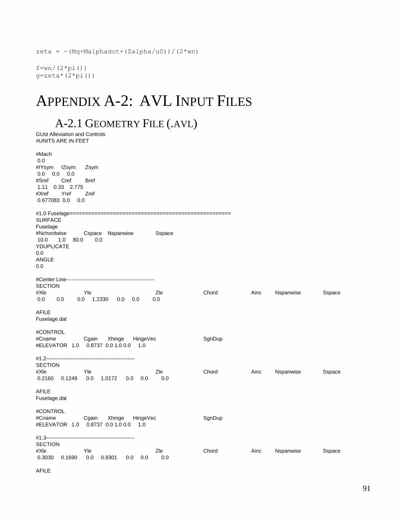
91
zeta = -(Mq+Malphadot+(Zalpha/u0))/(2*wn)
f=wn/(2*pi()) g=zeta*(2*pi())
APPENDIX A-2: AVL INPUT FILES
A-2.1 GEOMETRY FILE (.AVL) GUst Alleviation and Controls
#UNITS ARE IN FEET
#Mach
0.0
#IYsym IZsym Zsym
0.0 0.0 0.0
#Sref Cref Bref
1.11 0.33 2.775
#Xref Yref Zref
0.677083 0.0 0.0
#1.0 Fuselage====================================================
SURFACE
Fuselage
#Nchordwise Cspace Nspanwise Sspace
10.0 1.0 80.0 0.0
YDUPLICATE
0.0
ANGLE
0.0
#Center Line--------------------------------------------------
SECTION
#Xle Yle Zle Chord Ainc Nspanwise Sspace
0.0 0.0 0.0 1.2330 0.0 0.0 0.0
AFILE
Fuselage.dat
#CONTROL
#Cname Cgain Xhinge HingeVec SgnDup
#ELEVATOR 1.0 0.8737 0.0 1.0 0.0 1.0
#1.2--------------------------------------------------
SECTION
#Xle Yle Zle Chord Ainc Nspanwise Sspace
0.2160 0.1249 0.0 1.0172 0.0 0.0 0.0
AFILE
Fuselage.dat
#CONTROL
#Cname Cgain Xhinge HingeVec SgnDup
#ELEVATOR 1.0 0.8737 0.0 1.0 0.0 1.0
#1.3--------------------------------------------------
SECTION
#Xle Yle Zle Chord Ainc Nspanwise Sspace
0.3030 0.1690 0.0 0.9301 0.0 0.0 0.0
AFILE
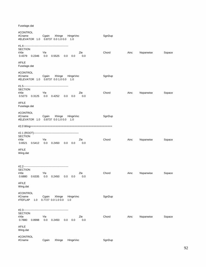
92
Fuselage.dat
#CONTROL
#Cname Cgain Xhinge HingeVec SgnDup
#ELEVATOR 1.0 0.8737 0.0 1.0 0.0 1.0
#1.4--------------------------------------------------
SECTION
#Xle Yle Zle Chord Ainc Nspanwise Sspace
0.4379 0.2346 0.0 0.5525 0.0 0.0 0.0
AFILE
Fuselage.dat
#CONTROL
#Cname Cgain Xhinge HingeVec SgnDup
#ELEVATOR 1.0 0.8737 0.0 1.0 0.0 1.0
#1.5--------------------------------------------------
SECTION
#Xle Yle Zle Chord Ainc Nspanwise Sspace
0.5273 0.3125 0.0 0.4252 0.0 0.0 0.0
AFILE
Fuselage.dat
#CONTROL
#Cname Cgain Xhinge HingeVec SgnDup
#ELEVATOR 1.0 0.8737 0.0 1.0 0.0 1.0
#2.0 Wing====================================================
#2.1 (ROOT)--------------------------------------------------
SECTION
#Xle Yle Zle Chord Ainc Nspanwise Sspace
0.6521 0.5412 0.0 0.2450 0.0 0.0 0.0
AFILE
Wing.dat
#2.2--------------------------------------------------
SECTION
#Xle Yle Zle Chord Ainc Nspanwise Sspace
0.6880 0.6335 0.0 0.2450 0.0 0.0 0.0
AFILE
Wing.dat
#CONTROL
#Cname Cgain Xhinge HingeVec SgnDup
#TEFLAP 1.0 0.7727 0.0 1.0 0.0 1.0
#2.3--------------------------------------------------
SECTION
#Xle Yle Zle Chord Ainc Nspanwise Sspace
0.7880 0.8998 0.0 0.2450 0.0 0.0 0.0
AFILE
Wing.dat
#CONTROL
#Cname Cgain Xhinge HingeVec SgnDup
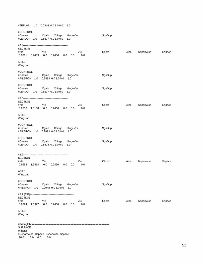
93
#TEFLAP 1.0 0.7946 0.0 1.0 0.0 1.0
#CONTROL
#Cname Cgain Xhinge HingeVec SgnDup
#LEFLAP 1.0 -0.8677 0.0 1.0 0.0 1.0
#2.4--------------------------------------------------
SECTION
#Xle Yle Zle Chord Ainc Nspanwise Sspace
0.8081 0.9433 0.0 0.2450 0.0 0.0 0.0
AFILE
Wing.dat
#CONTROL
#Cname Cgain Xhinge HingeVec SgnDup
#AILERON 1.0 0.7813 0.0 1.0 0.0 1.0
#CONTROL
#Cname Cgain Xhinge HingeVec SgnDup
#LEFLAP 1.0 -0.8677 0.0 1.0 0.0 1.0
#2.5--------------------------------------------------
SECTION
#Xle Yle Zle Chord Ainc Nspanwise Sspace
0.9530 1.3168 0.0 0.2450 0.0 0.0 0.0
AFILE
Wing.dat
#CONTROL
#Cname Cgain Xhinge HingeVec SgnDup
#AILERON 1.0 0.7813 0.0 1.0 0.0 1.0
#CONTROL
#Cname Cgain Xhinge HingeVec SgnDup
#LEFLAP 1.0 -0.8678 0.0 1.0 0.0 1.0
#2.6--------------------------------------------------
SECTION
#Xle Yle Zle Chord Ainc Nspanwise Sspace
0.9593 1.3414 0.0 0.2450 0.0 0.0 0.0
AFILE
Wing.dat
#CONTROL
#Cname Cgain Xhinge HingeVec SgnDup
#AILERON 1.0 0.7948 0.0 1.0 0.0 1.0
#2.7 (TIP)--------------------------------------------------
SECTION
#Xle Yle Zle Chord Ainc Nspanwise Sspace
0.9824 1.3927 0.0 0.2450 0.0 0.0 0.0
AFILE
Wing.dat
#3Winglet===================================================
SURFACE
Winglet
#Nchordwise Cspace Nspanwise Sspace
10.0 3.0 0.0 0.0
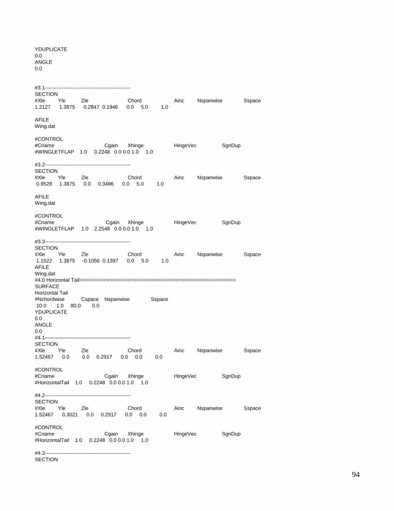
94
YDUPLICATE
0.0
ANGLE
0.0
#3.1--------------------------------------------------
SECTION
#Xle Yle Zle Chord Ainc Nspanwise Sspace
1.2127 1.3875 0.2847 0.1946 0.0 5.0 1.0
AFILE
Wing.dat
#CONTROL
#Cname Cgain Xhinge HingeVec SgnDup
#WINGLETFLAP 1.0 0.2248 0.0 0.0 1.0 1.0
#3.2--------------------------------------------------
SECTION
#Xle Yle Zle Chord Ainc Nspanwise Sspace
0.9528 1.3875 0.0 0.3496 0.0 5.0 1.0
AFILE
Wing.dat
#CONTROL
#Cname Cgain Xhinge HingeVec SgnDup
#WINGLETFLAP 1.0 2.2548 0.0 0.0 1.0 1.0
#3.3--------------------------------------------------
SECTION
#Xle Yle Zle Chord Ainc Nspanwise Sspace
1.1522 1.3875 -0.1056 0.1397 0.0 5.0 1.0
AFILE
Wing.dat
#4.0 Horizontal Tail====================================================
SURFACE
Horizontal Tail
#Nchordwise Cspace Nspanwise Sspace
10.0 1.0 80.0 0.0
YDUPLICATE
0.0
ANGLE
0.0
#4.1--------------------------------------------------
SECTION
#Xle Yle Zle Chord Ainc Nspanwise Sspace
1.52467 0.0 0.0 0.2917 0.0 0.0 0.0
#CONTROL
#Cname Cgain Xhinge HingeVec SgnDup
#HorizontalTail 1.0 0.2248 0.0 0.0 1.0 1.0
#4.2--------------------------------------------------
SECTION
#Xle Yle Zle Chord Ainc Nspanwise Sspace
1.52467 0.3021 0.0 0.2917 0.0 0.0 0.0
#CONTROL
#Cname Cgain Xhinge HingeVec SgnDup
#HorizontalTail 1.0 0.2248 0.0 0.0 1.0 1.0
#4.3--------------------------------------------------
SECTION
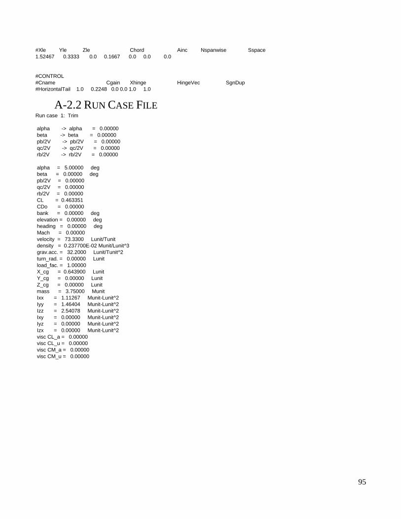
95
#Xle Yle Zle Chord Ainc Nspanwise Sspace
1.52467 0.3333 0.0 0.1667 0.0 0.0 0.0
#CONTROL
#Cname Cgain Xhinge HingeVec SgnDup
#HorizontalTail 1.0 0.2248 0.0 0.0 1.0 1.0
A-2.2 RUN CASE FILE Run case 1: Trim
alpha -> alpha = 0.00000
beta -> beta = 0.00000
pb/2V -> pb/2V = 0.00000
qc/2V -> qc/2V = 0.00000
rb/2V -> rb/2V = 0.00000
alpha = 5.00000 deg
beta = 0.00000 deg
pb/2V = 0.00000
qc/2V = 0.00000
rb/2V = 0.00000
CL = 0.463351
CDo = 0.00000
bank = 0.00000 deg
elevation = 0.00000 deg
heading = 0.00000 deg
Mach = 0.00000
velocity = 73.3300 Lunit/Tunit
density = 0.237700E-02 Munit/Lunit^3
grav.acc. = 32.2000 Lunit/Tunit^2
turn_rad. = 0.00000 Lunit
load_fac. = 1.00000
X_cg = 0.643900 Lunit
Y_cg = 0.00000 Lunit
Z_cg = 0.00000 Lunit
mass = 3.75000 Munit
Ixx = 1.11267 Munit-Lunit^2
Iyy = 1.46404 Munit-Lunit^2
Izz = 2.54078 Munit-Lunit^2
Ixy = 0.00000 Munit-Lunit^2
Iyz = 0.00000 Munit-Lunit^2
Izx = 0.00000 Munit-Lunit^2
visc CL_a = 0.00000
visc CL_u = 0.00000
visc CM_a = 0.00000
visc CM_u = 0.00000
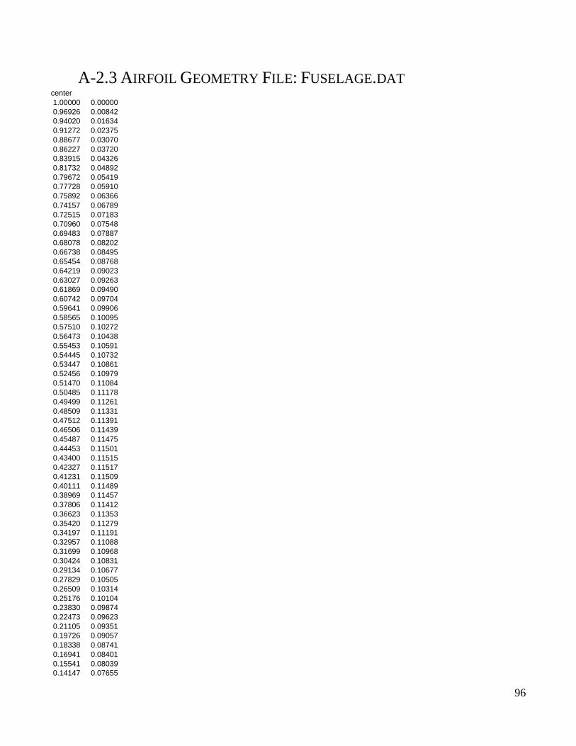
96
A-2.3 AIRFOIL GEOMETRY FILE: FUSELAGE.DAT center
1.00000 0.00000
0.96926 0.00842
0.94020 0.01634
0.91272 0.02375
0.88677 0.03070
0.86227 0.03720
0.83915 0.04326
0.81732 0.04892
0.79672 0.05419
0.77728 0.05910
0.75892 0.06366
0.74157 0.06789
0.72515 0.07183
0.70960 0.07548
0.69483 0.07887
0.68078 0.08202
0.66738 0.08495
0.65454 0.08768
0.64219 0.09023
0.63027 0.09263
0.61869 0.09490
0.60742 0.09704
0.59641 0.09906
0.58565 0.10095
0.57510 0.10272
0.56473 0.10438
0.55453 0.10591
0.54445 0.10732
0.53447 0.10861
0.52456 0.10979
0.51470 0.11084
0.50485 0.11178
0.49499 0.11261
0.48509 0.11331
0.47512 0.11391
0.46506 0.11439
0.45487 0.11475
0.44453 0.11501
0.43400 0.11515
0.42327 0.11517
0.41231 0.11509
0.40111 0.11489
0.38969 0.11457
0.37806 0.11412
0.36623 0.11353
0.35420 0.11279
0.34197 0.11191
0.32957 0.11088
0.31699 0.10968
0.30424 0.10831
0.29134 0.10677
0.27829 0.10505
0.26509 0.10314
0.25176 0.10104
0.23830 0.09874
0.22473 0.09623
0.21105 0.09351
0.19726 0.09057
0.18338 0.08741
0.16941 0.08401
0.15541 0.08039
0.14147 0.07655
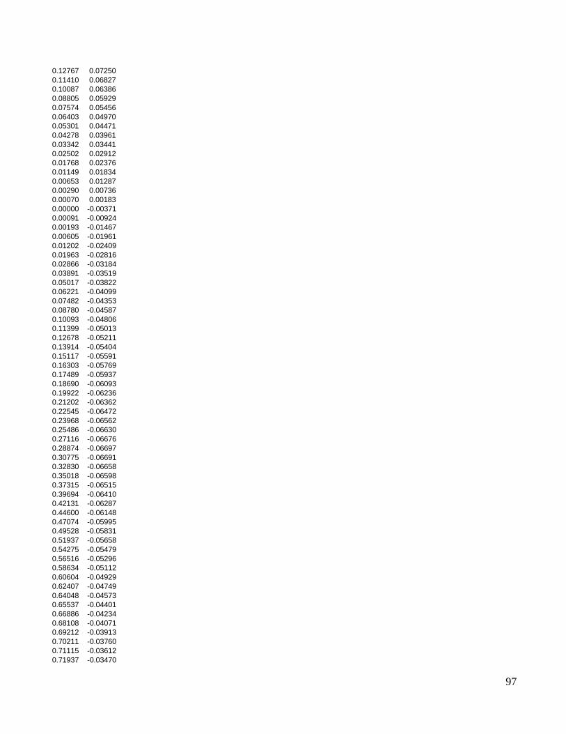
97
0.12767 0.07250
0.11410 0.06827
0.10087 0.06386
0.08805 0.05929
0.07574 0.05456
0.06403 0.04970
0.05301 0.04471
0.04278 0.03961
0.03342 0.03441
0.02502 0.02912
0.01768 0.02376
0.01149 0.01834
0.00653 0.01287
0.00290 0.00736
0.00070 0.00183
0.00000 -0.00371
0.00091 -0.00924
0.00193 -0.01467
0.00605 -0.01961
0.01202 -0.02409
0.01963 -0.02816
0.02866 -0.03184
0.03891 -0.03519
0.05017 -0.03822
0.06221 -0.04099
0.07482 -0.04353
0.08780 -0.04587
0.10093 -0.04806
0.11399 -0.05013
0.12678 -0.05211
0.13914 -0.05404
0.15117 -0.05591
0.16303 -0.05769
0.17489 -0.05937
0.18690 -0.06093
0.19922 -0.06236
0.21202 -0.06362
0.22545 -0.06472
0.23968 -0.06562
0.25486 -0.06630
0.27116 -0.06676
0.28874 -0.06697
0.30775 -0.06691
0.32830 -0.06658
0.35018 -0.06598
0.37315 -0.06515
0.39694 -0.06410
0.42131 -0.06287
0.44600 -0.06148
0.47074 -0.05995
0.49528 -0.05831
0.51937 -0.05658
0.54275 -0.05479
0.56516 -0.05296
0.58634 -0.05112
0.60604 -0.04929
0.62407 -0.04749
0.64048 -0.04573
0.65537 -0.04401
0.66886 -0.04234
0.68108 -0.04071
0.69212 -0.03913
0.70211 -0.03760
0.71115 -0.03612
0.71937 -0.03470
98
0.72686 -0.03333
0.73376 -0.03203
0.74017 -0.03078
0.74620 -0.02961
0.75197 -0.02849
0.75754 -0.02744
0.76297 -0.02642
0.76834 -0.02545
0.77371 -0.02449
0.77914 -0.02355
0.78470 -0.02261
0.79044 -0.02167
0.79645 -0.02070
0.80277 -0.01970
0.80949 -0.01867
0.81665 -0.01758
0.82433 -0.01643
0.83259 -0.01521
0.84149 -0.01394
0.85110 -0.01262
0.86148 -0.01129
0.87269 -0.00994
0.88480 -0.00861
0.89787 -0.00731
0.91196 -0.00605
0.92714 -0.00486
0.94347 -0.00374
0.96102 -0.00272
0.97984 -0.00181
1.00000 -0.00103
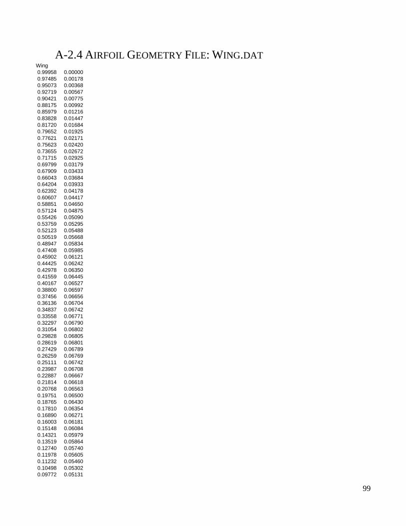
99
A-2.4 AIRFOIL GEOMETRY FILE: WING.DAT Wing
0.99958 0.00000
0.97485 0.00178
0.95073 0.00368
0.92719 0.00567
0.90421 0.00775
0.88175 0.00992
0.85979 0.01216
0.83828 0.01447
0.81720 0.01684
0.79652 0.01925
0.77621 0.02171
0.75623 0.02420
0.73655 0.02672
0.71715 0.02925
0.69799 0.03179
0.67909 0.03433
0.66043 0.03684
0.64204 0.03933
0.62392 0.04178
0.60607 0.04417
0.58851 0.04650
0.57124 0.04875
0.55426 0.05090
0.53759 0.05295
0.52123 0.05488
0.50519 0.05668
0.48947 0.05834
0.47408 0.05985
0.45902 0.06121
0.44425 0.06242
0.42978 0.06350
0.41559 0.06445
0.40167 0.06527
0.38800 0.06597
0.37456 0.06656
0.36136 0.06704
0.34837 0.06742
0.33558 0.06771
0.32297 0.06790
0.31054 0.06802
0.29828 0.06805
0.28619 0.06801
0.27429 0.06789
0.26259 0.06769
0.25111 0.06742
0.23987 0.06708
0.22887 0.06667
0.21814 0.06618
0.20768 0.06563
0.19751 0.06500
0.18765 0.06430
0.17810 0.06354
0.16890 0.06271
0.16003 0.06181
0.15148 0.06084
0.14321 0.05979
0.13519 0.05864
0.12740 0.05740
0.11978 0.05605
0.11232 0.05460
0.10498 0.05302
0.09772 0.05131
100
0.09052 0.04947
0.08333 0.04749
0.07614 0.04535
0.06890 0.04306
0.06161 0.04060
0.05432 0.03799
0.04714 0.03525
0.04016 0.03239
0.03346 0.02942
0.02713 0.02636
0.02126 0.02323
0.01595 0.02004
0.01129 0.01681
0.00736 0.01354
0.00426 0.01027
0.00207 0.00700
0.00089 0.00374
0.00000 -0.00118
0.00042 -0.00320
0.00120 -0.00513
0.00232 -0.00697
0.00375 -0.00873
0.00549 -0.01042
0.00752 -0.01202
0.00981 -0.01356
0.01235 -0.01502
0.01512 -0.01642
0.01811 -0.01776
0.02129 -0.01904
0.02466 -0.02026
0.02818 -0.02143
0.03185 -0.02255
0.03564 -0.02362
0.03954 -0.02465
0.04352 -0.02564
0.04758 -0.02660
0.05170 -0.02752
0.05589 -0.02842
0.06019 -0.02928
0.06465 -0.03011
0.06932 -0.03090
0.07425 -0.03167
0.07947 -0.03240
0.08504 -0.03309
0.09100 -0.03375
0.09740 -0.03437
0.10429 -0.03496
0.11171 -0.03551
0.11970 -0.03603
0.12832 -0.03650
0.13761 -0.03694
0.14762 -0.03734
0.15839 -0.03770
0.16996 -0.03802
0.18239 -0.03829
0.19573 -0.03853
0.20999 -0.03873
0.22512 -0.03888
0.24105 -0.03900
0.25771 -0.03908
0.27501 -0.03912
0.29288 -0.03914
0.31125 -0.03912
0.33004 -0.03907
0.34918 -0.03899

101
0.36859 -0.03888
0.38820 -0.03875
0.40793 -0.03860
0.42770 -0.03843
0.44745 -0.03823
0.46709 -0.03802
0.48655 -0.03779
0.50576 -0.03755
0.52464 -0.03730
0.54312 -0.03703
0.56112 -0.03675
0.57869 -0.03646
0.59598 -0.03611
0.61314 -0.03570
0.63035 -0.03520
0.64774 -0.03458
0.66549 -0.03382
0.68374 -0.03289
0.70267 -0.03177
0.72241 -0.03045
0.74314 -0.02888
0.76502 -0.02705
0.78819 -0.02494
0.81281 -0.02252
0.83905 -0.01976
0.86707 -0.01665
0.89701 -0.01316
0.92904 -0.00926
0.96332 -0.00493
1.00000 -0.00015
102
APPENDIX A-3: PROPOSAL
Senior Project Proposal
TEAM:
GUst Alleviation Control (2014-15)
TEAM MEMBERS:
Tuan Dinh Jr [email protected] (909) 720-2532 Team Lead
Dwight Nava [email protected] (213) 400-0395 Deputy
Reginald Guinto [email protected] (909) 539-5090
George Paguio [email protected] (213) 304-5036
Tanner Clark [email protected] (661) 219-3943
Jason Kong [email protected] (626) 660-7603
Dong Jin Ryoo [email protected] (714) 873-2572
Arya WIlliams [email protected] (626) 710-0219
Bill Wogahn [email protected] (909) 993-2897
CONSULTANT AND SUPPORT TEAM:
Evan Robert Johnson [email protected] (714) 851-4146
Crystal Nunez [email protected] (714) 619-1434
Anahi Hernandez [email protected] (323) 490-2959
Faculty Advisor: Professor Steven K. Dobbs
Submission Date: October 2014
Approved: ______________________________________________, Date _________________
AEROSPACE ENGINEERING DEPARTMENT
CALIFORNIA POLYTECHNIC UNIVERSITY, POMONA
103
1.0 NEED AND BENEFITS OF THE PROJECT:
1.1 Next generation aircrafts are implementing higher AR wings (Blended Wing Bodies). Further
research on aero-elastic phenomena, specifically the analysis of flutter and gust response
challenges, will contribute to creating successful next generation aircrafts.
1.2 Of the four major aerospace engineering disciplines, control systems offers the least
undergraduate courses despite having become one of the most important disciplines in industry.
This project allows for a greater understanding of advanced control topics not covered in any
undergraduate course.
1.3 If the department were to include practices and test procedures from this project in the
aerospace curriculum in the form of a lab, undergraduate students would be exposed to data
acquisition and controls hardware.
1.4 Students will be provided with hands on experience with testing a blended wing-body’s
Stability Augmentation System (SAS).
2.0 PRIMARY PROJECT OBJECTIVES:
2.1 Modifying the blended wing body model fabricated by the 2013-2014 FALCON Club senior
project team. The modified X-56 will have a relocated C.G by the use of a nose boom weight in
front of the model. The goal of this is to move the AC aft of the C.G. for static and dynamic
stability.
2.2 The FALCON (Flutter ALleviation and CONtrol) model will be tested in the subsonic wind
tunnel with two degrees of freedom for longitudinal stability testing in order to develop an
optimized longitudinal Stability Augmentation control system.
2.3 Demonstrate a longitudinal gust alleviation system capable of reacting to vertical gusts in the
subsonic wind tunnel. This test will utilize the gust generation system designed and installed in
the wind tunnel by the 2012-2013 Flutter Club team.
2.4 Expand stability augmentation system to include lateral-directional motion. Demonstrate
controllability and augmented static and dynamic stability of a blended wing-body aircraft in
five degree of freedom motion.
104
2.5 Super impose the stability augmentation system with gust alleviation system to reduce flutter
phenomena for a rigid wing structure.
2.6 Perform preliminary vibration and flutter analysis in NASTRAN for a composite-skinned
flexible wing optimized for span wise torsional bending. Determine optimal material, wing
structure, and mass distribution to obtain desired structural dynamic modes.
3.0 SECONDARY PROJECT OBJECTIVES:
3.1 Explore and test alternative control methods for a blended wing-body aircraft. Utilize
differential rudder and aileron actuation in order to aid in yawing motion through differential
drag effects.
3.2 Demonstrate the feasibility of a remotely processed control system running on a portable
computer running a real-time Simulink control system.
3.3 Provide the Aerospace Engineering department with a fully functional flutter research model
capable of modeling advanced control concepts aimed at actively suppressing aero-elastic flutter
during simulated flight in the low-speed wind tunnel.
4.0 PRODUCTS OF PROJECT:
4.1 New updates to the FALCON platform including a variable C.G. through the use of a nose
boom weight, as well as a horizontal tail with elevator and vertical tails with rudder for an
increase in control surface sensitivity.
4.2 Valuable research for real time stabilization of an unstable blended wing body aircraft. Included
in this research is the capability of stabilizing an aircraft that uses flexible, lightweight
composite wings.
5.0 METHODS TO MEET PROJECT
105
OBJECTIVES:
5.1 Laboratory Use Required:
Aerospace Engineering Department Low Speed Wind Tunnel
Structures Laboratory
UAV Laboratory
Thermal Fluids Laboratory
5.2 Experiments and Tests:
5.2.1 Stable static margin
Determine location of the C.G. with respect to the nose boom weight.
Hand calculation of expected aerodynamic center.
Graphical representation between C.G. and nose boom weight location with respect to
the calculated A.C.
5.2.2 Flight Testing:
Implement a tail (if necessary) to create a bigger moment arm for more effective
aerodynamic control of trim and stability.
Develop a longitudinal Stability Augmentation System.
Introduce a gust alleviation system using the SAS.
5.3 Equipment Needed for Project:
ArduPilot Mega 2.5 integrated flight management system
High speed ADC (Analog to Digital) equipment.
Wire resistance strain gauges.
Accelerometer/Gyroscope packages. (Inertial Measurement Units)
Low-speed wind tunnel 5-DOF gimbal mount.
Vibrational analysis equipment:
OROS Dynamic Analysis Hammer
5.4 Computer Software Required:
Solid Works 3D modeling and analysis software.
Athena Vortex Lattice
NASTRAN structural analysis software.
MATLAB control simulation software:
SIMULINK Real-Time Libraries
SIMULINK Code Generation Packages
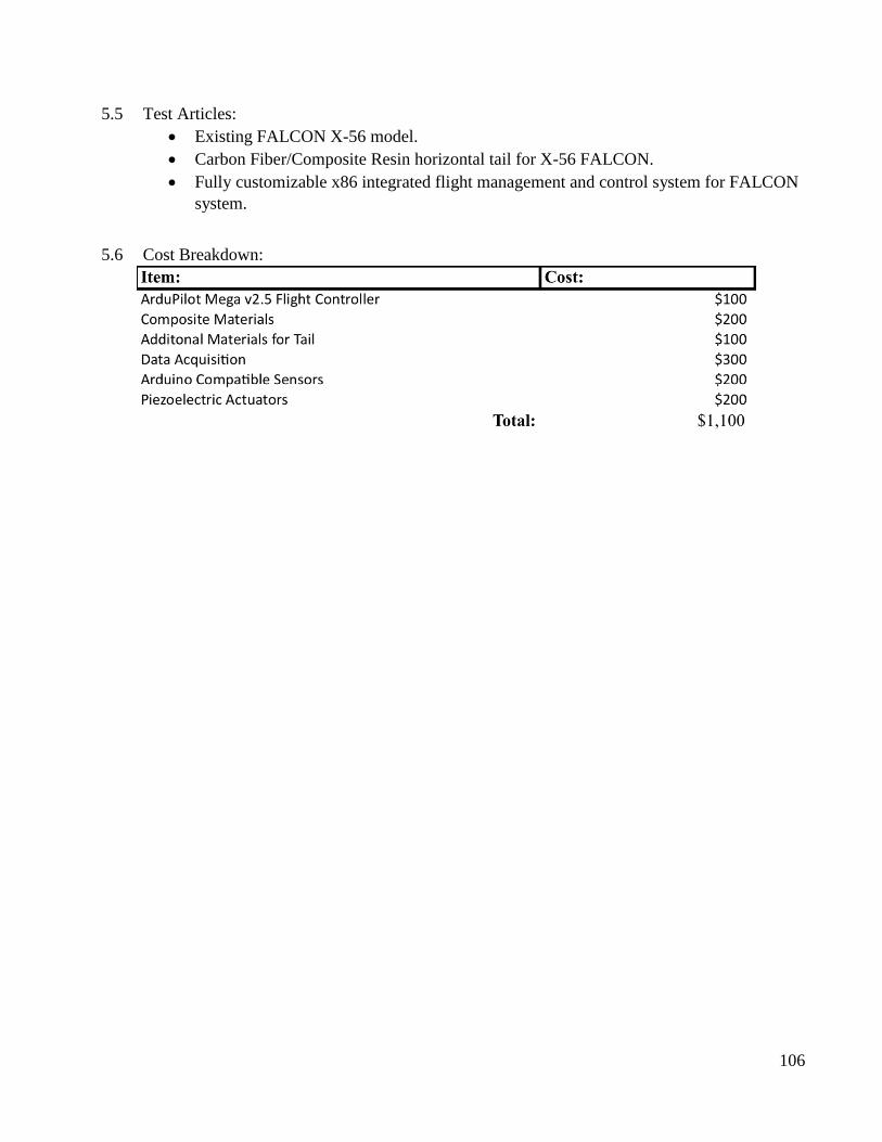
106
5.5 Test Articles:
Existing FALCON X-56 model.
Carbon Fiber/Composite Resin horizontal tail for X-56 FALCON.
Fully customizable x86 integrated flight management and control system for FALCON
system.
5.6 Cost Breakdown:

107
5.7 Sources of Funding
Program Who is eligible
to apply
Purpose Funds for
Student
Funds For
Faculty
Deadlines
Engineering
Scholars
Program (ESP)
Engineering
majors, Pell
Grant eligible
Conduct UR and
prepare for
graduate school
and career
development
$5,000 per
Academic Year
N/A October 14th
Spring 2015
Recruitment for
continuing
students for
2015-16
Academic Year
President’s
Special Travel
Fund
ALL students,
All colleges all
majors
Travels to
present at
conferences
Up to $1,000
(registration,
Transportation,
Hotel)
Conference Fee
Registration
October 20th
Kellog
Undergraduates
Scholar Program
Low income, FG,
and military
veterans. GPA of
2.7 or higher
Faculty mentored
research projects
Up to $2000 per
Academic Year
See Kellog
Future Mini
Grant
November 6th
Kellog Future
Mini-Grants
Faculty and their
student research
treams
Minor
equipment,
software,
research travel
At discretion of
faculty mentor
Up to 2000 per
academic year
November 6th
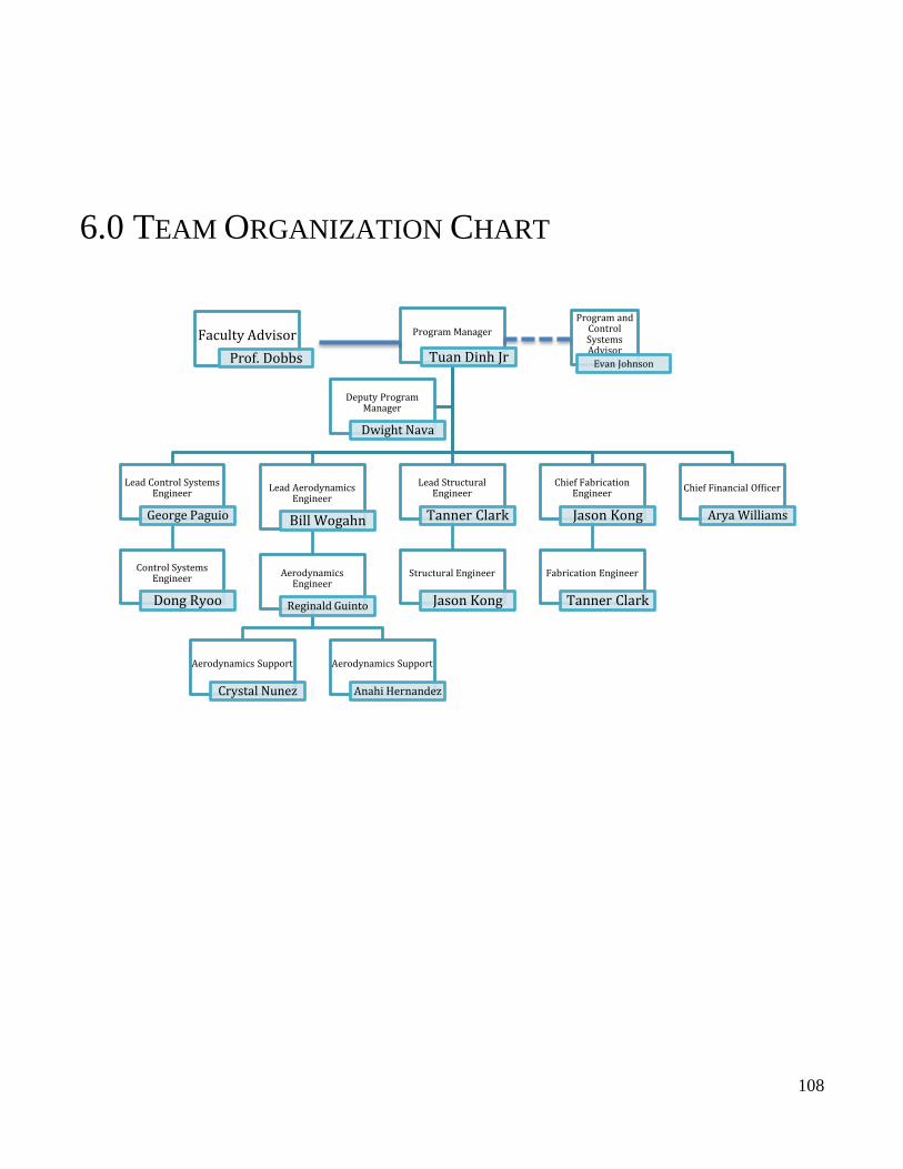
108
6.0 TEAM ORGANIZATION CHART
Program Manager
Tuan Dinh Jr
Lead Control Systems Engineer
George Paguio
Control Systems Engineer
Dong Ryoo
Lead Aerodynamics Engineer
Bill Wogahn
Aerodynamics Engineer
Reginald Guinto
Aerodynamics Support
Crystal Nunez
Aerodynamics Support
Anahi Hernandez
Lead Structural Engineer
Tanner Clark
Structural Engineer
Jason Kong
Chief Fabrication Engineer
Jason Kong
Fabrication Engineer
Tanner Clark
Chief Financial Officer
Arya Williams
Deputy Program Manager
Dwight Nava
Program and Control Systems Advisor
Evan Johnson
Faculty Advisor
Prof. Dobbs

109
7.0 KEY RISKS TO MEETING OBJECTIVES –
MITIGATION PLAN 7.2 Horizontal tail structural failure
Do structural test for the composite rods
Lay up the plywood with a composite skin
Trade studies on materials
7.3 Inadequate funding
Come up with additional funding options.
If necessary fund project costs out of pocket
7.4 Inadequate training in autonomous stability control systems
Contact Evan Johnson for a briefing about autonomous stability control systems
Do research on autonomous stability control systems
8.0 SCHEDULE OF MAJOR PROJECT MILESTONES
Name Start Finish % Complete
Assemble Team Sep 30 2014 Oct 10 2014 100
Proposal Due Sep 30 2014 Oct 30 2014 100
Static Margin Test Oct 16 2014 Oct 27 2014 50
Perform structural modifications Oct 17 2014 Nov 11 2014
Wind tunnel test #1 w/ Tail (open loop) Nov 10 2014 Nov 24 2014
Fall Quarter Interim Report Oct 16 2014 Dec 1 2014
Develop optimized longitudinal Stability
Augmentation System Oct 13 2014 Jan 31 2015
Wind tunnel test #2 w/ Tail (closed loop “S.A.S”) Feb 1 2015 Feb 28 2015
Winter Quarter Interim Report Jan 5 2015 Mar 13 2015
Develop longitudinal Gust Alleviation System Mar 23 2015 Apr 1 2015
Wind tunnel test #3 w/ Tail (closed loop “G.A.S”)
in Gust flow Apr 1 2015 May 1 2015
Final Report Draft May 1 2015 May 27 2015
Final Report Approved June 1 2015
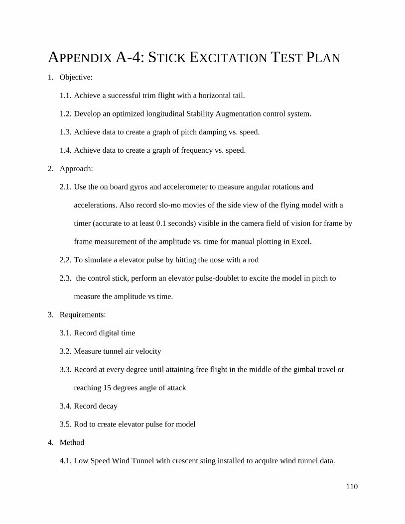
110
APPENDIX A-4: STICK EXCITATION TEST PLAN 1. Objective:
1.1. Achieve a successful trim flight with a horizontal tail.
1.2. Develop an optimized longitudinal Stability Augmentation control system.
1.3. Achieve data to create a graph of pitch damping vs. speed.
1.4. Achieve data to create a graph of frequency vs. speed.
2. Approach:
2.1. Use the on board gyros and accelerometer to measure angular rotations and
accelerations. Also record slo-mo movies of the side view of the flying model with a
timer (accurate to at least 0.1 seconds) visible in the camera field of vision for frame by
frame measurement of the amplitude vs. time for manual plotting in Excel.
2.2. To simulate a elevator pulse by hitting the nose with a rod
2.3. the control stick, perform an elevator pulse-doublet to excite the model in pitch to
measure the amplitude vs time.
3. Requirements:
3.1. Record digital time
3.2. Measure tunnel air velocity
3.3. Record at every degree until attaining free flight in the middle of the gimbal travel or
reaching 15 degrees angle of attack
3.4. Record decay
3.5. Rod to create elevator pulse for model
4. Method
4.1. Low Speed Wind Tunnel with crescent sting installed to acquire wind tunnel data.
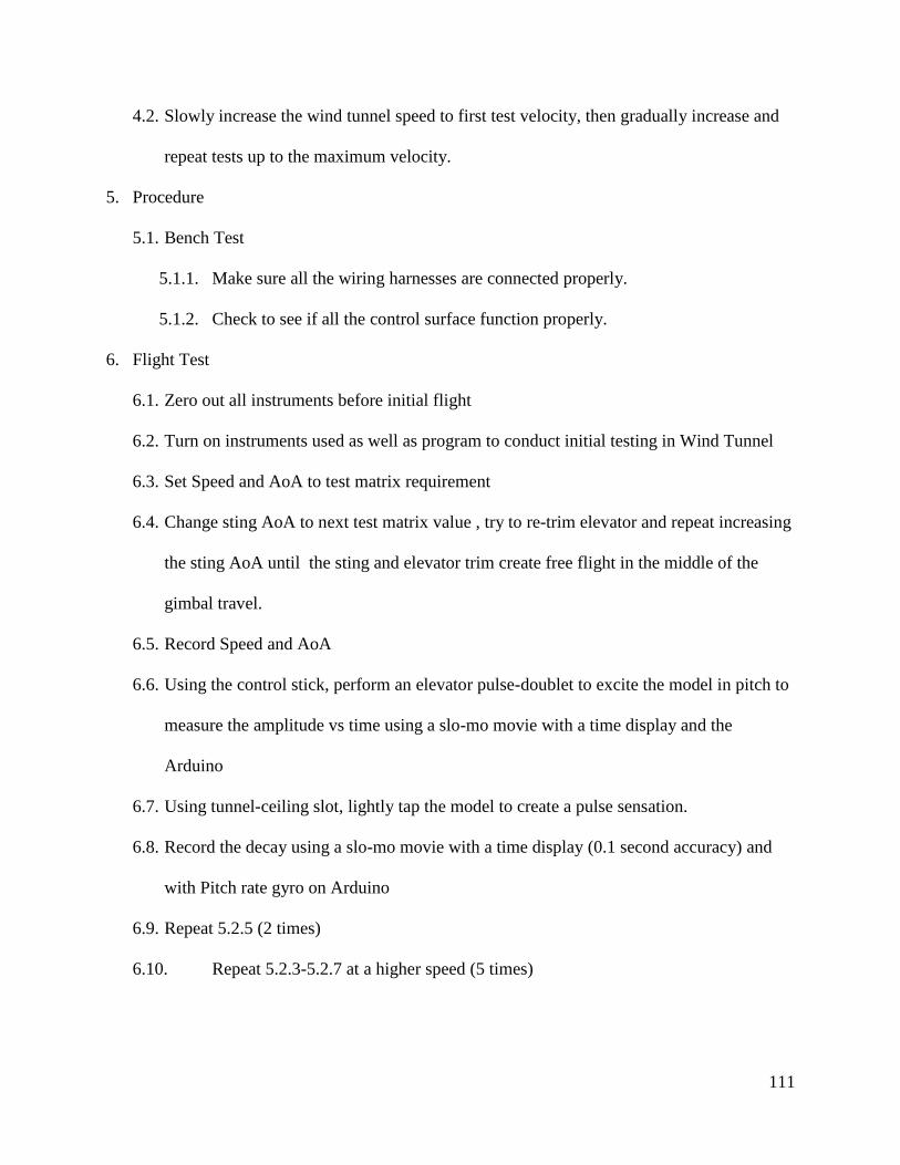
111
4.2. Slowly increase the wind tunnel speed to first test velocity, then gradually increase and
repeat tests up to the maximum velocity.
5. Procedure
5.1. Bench Test
5.1.1. Make sure all the wiring harnesses are connected properly.
5.1.2. Check to see if all the control surface function properly.
6. Flight Test
6.1. Zero out all instruments before initial flight
6.2. Turn on instruments used as well as program to conduct initial testing in Wind Tunnel
6.3. Set Speed and AoA to test matrix requirement
6.4. Change sting AoA to next test matrix value , try to re-trim elevator and repeat increasing
the sting AoA until the sting and elevator trim create free flight in the middle of the
gimbal travel.
6.5. Record Speed and AoA
6.6. Using the control stick, perform an elevator pulse-doublet to excite the model in pitch to
measure the amplitude vs time using a slo-mo movie with a time display and the
Arduino
6.7. Using tunnel-ceiling slot, lightly tap the model to create a pulse sensation.
6.8. Record the decay using a slo-mo movie with a time display (0.1 second accuracy) and
with Pitch rate gyro on Arduino
6.9. Repeat 5.2.5 (2 times)
6.10. Repeat 5.2.3-5.2.7 at a higher speed (5 times)
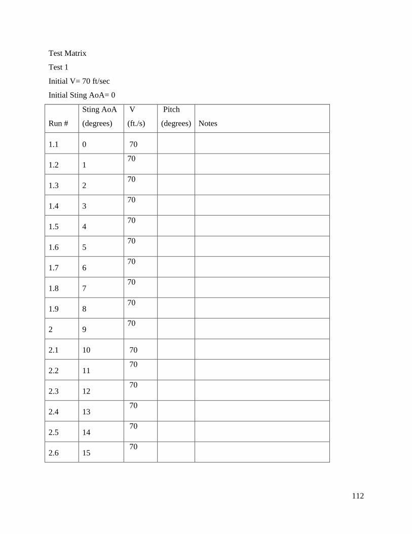
112
Test Matrix
Test 1
Initial V= 70 ft/sec
Initial Sting AoA= 0
Run #
Sting AoA
(degrees)
V
(ft./s)
Pitch
(degrees) Notes
1.1 0 70
1.2 1 70
1.3 2 70
1.4 3 70
1.5 4 70
1.6 5 70
1.7 6 70
1.8 7 70
1.9 8 70
2 9 70
2.1 10 70
2.2 11 70
2.3 12 70
2.4 13 70
2.5 14 70
2.6 15 70
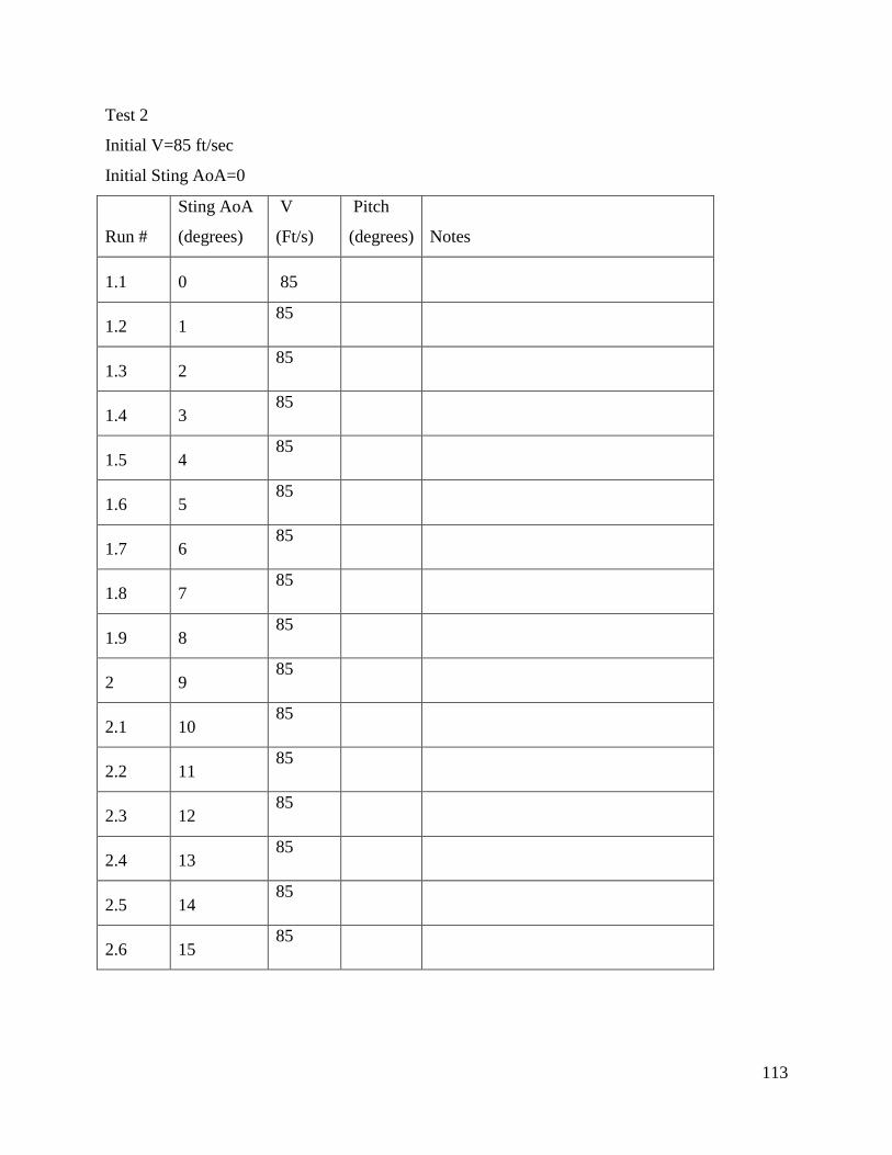
113
Test 2
Initial V=85 ft/sec
Initial Sting AoA=0
Run #
Sting AoA
(degrees)
V
(Ft/s)
Pitch
(degrees) Notes
1.1 0 85
1.2 1 85
1.3 2 85
1.4 3 85
1.5 4 85
1.6 5 85
1.7 6 85
1.8 7 85
1.9 8 85
2 9 85
2.1 10 85
2.2 11 85
2.3 12 85
2.4 13 85
2.5 14 85
2.6 15 85

114
Test 3
Initial V= 100 ft/sec
Initial AoA=
Run #
Sting AoA
(degrees)
V
(Ft/s)
Pitch
(degrees) Notes
1.1 0 100
1.2 1 100
1.3 2 100
1.4 3 100
1.5 4 100
1.6 5 100
1.7 6 100
1.8 7 100
1.9 8 100
2 9 100
2.1 10 100
2.2 11 100
2.3 12 100
2.4 13 100
2.5 14 100
2.6 15 100
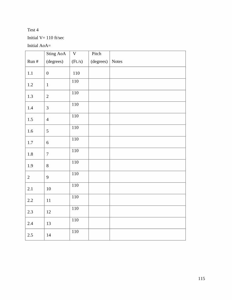
115
Test 4
Initial V= 110 ft/sec
Initial AoA=
Run #
Sting AoA
(degrees)
V
(Ft./s)
Pitch
(degrees) Notes
1.1 0 110
1.2 1 110
1.3 2 110
1.4 3 110
1.5 4 110
1.6 5 110
1.7 6 110
1.8 7 110
1.9 8 110
2 9 110
2.1 10 110
2.2 11 110
2.3 12 110
2.4 13 110
2.5 14 110