semiparametric mixed models for increment-averaged data with application to carbon sequestration in...

Semiparametric Mixed Models for Increment-Averaged Data with Application to CarbonSequestration in Agricultural SoilsAuthor(s): F. Jay Breidt, Nan-Jung Hsu and Stephen OgleSource: Journal of the American Statistical Association, Vol. 102, No. 479 (Sep., 2007), pp. 803-812Published by: American Statistical AssociationStable URL: http://www.jstor.org/stable/27639926 .

Accessed: 14/06/2014 07:44

Your use of the JSTOR archive indicates your acceptance of the Terms & Conditions of Use, available at .http://www.jstor.org/page/info/about/policies/terms.jsp

.JSTOR is a not-for-profit service that helps scholars, researchers, and students discover, use, and build upon a wide range ofcontent in a trusted digital archive. We use information technology and tools to increase productivity and facilitate new formsof scholarship. For more information about JSTOR, please contact [email protected].

.

American Statistical Association is collaborating with JSTOR to digitize, preserve and extend access to Journalof the American Statistical Association.

http://www.jstor.org

This content downloaded from 91.229.248.67 on Sat, 14 Jun 2014 07:44:10 AMAll use subject to JSTOR Terms and Conditions

http://www.jstor.org/action/showPublisher?publisherCode=astata

http://www.jstor.org/stable/27639926?origin=JSTOR-pdf

http://www.jstor.org/page/info/about/policies/terms.jsp


Semiparametric Mixed Models for

Increment-Averaged Data With Application to Carbon Sequestration in Agricultural Soils

F. Jay Breidt, Nan-Jung Hsu, and Stephen Ogle

Adoption of conservation tillage practice in agriculture offers the potential to mitigate greenhouse gas emissions. Studies comparing conser

vation tillage methods to traditional tillage pair fields under the two management systems and obtain soil core samples from each treatment.

Cores are divided into multiple increments, and matching increments from one or more cores are aggregated and analyzed for carbon stock. These data represent not the actual value at a specific depth, but rather the total or average over a depth increment. A semiparametric mixed model is developed for such increment-averaged data. The model uses parametric fixed effects to represent covariate effects, random effects to capture correlation within studies, and an integrated smooth function to describe effects of depth. The depth function is specified as an

additive model, estimated with penalized splines using standard mixed model software. Smoothing parameters are automatically selected

using restricted maximum likelihood. The methodology is applied to the problem of estimating a change in carbon stock due to a change in

tillage practice.

KEY WORDS: Core sample; Greenhouse gas; Nonparametric regression; Ornstein-Uhlenbeck process; Penalized spline; Restricted max

imum likelihood; Varying-coefficient model.

1. INTRODUCTION

Traditional agricultural management uses tillage to turn over

the soil and bury postharvest crop residues, often several times

before planting. Recently, "no-till" production systems that do

not use tillage have become economically feasible due to new

techniques and equipment. No-till, in which crop residues are

left on the soil surface, reduces soil losses due to wind and wa

ter erosion (Lindstrom, Schumacher, Cogo, and Blecha 1998). This in turn reduces the flow of sediments, nutrients, and pes

ticides into surface waters. In addition, no-till enhances soil or

ganic matter due to reduced soil disturbance (Six, Elliot, Paus

tian, and Doran 1998) and over time may improve soil fertility. Furthermore, no-till may result in lower production costs, due

to fewer management steps and lower machinery costs. (Con

ventional tillage requires more expensive, higher horsepower

tractors.) "Reduced-till" systems limit tillage and other soil

disturbing activities and leave substantial residue on the soil

surface, but to a lesser extent than no-till. Reduced-till systems

offer many of the same advantages as no-till. Together, these

systems are known as "conservation tillage" methods (Kern and

Johnson 1993; U.S. Department of Agriculture 1994). Recent interest in conservation tillage has focused on its

potential for reducing greenhouse gas (GHG) emissions, be cause of reduced soil disturbance that leads to more carbon

storage in the profile, particularly in no-till systems (Kern and Johnson 1993; Paustian et al. 1997; Lai, Kimble, Fol

lett, and Cole 1998; Smith, Powlson, Smith, Falloon, and Coleman 2000). The amount of carbon sequestered due to a

change in tillage system is economically as well as environmen

tally important; for example, the Chicago Climate Exchange

F. Jay Breidt is Professor, Department of Statistics, Colorado State Uni

versity, Fort Collins, CO 80523 (E-mail: [email protected]). Nan-Jung Hsu is Associate Professor, Institute of Statistics, National Tsing-Hua Univer

sity, Hsin-Chu, Taiwan 30043 (E-mail: [email protected]). Stephen Ogle is Research Scientist, Natural Resource Ecology Laboratory, Colorado State

University, Fort Collins, CO 80523 (E-mail: [email protected]). The work reported here was developed under STAR Research Assistance Agree ment CR-829095 awarded by the U.S. Environmental Protection Agency (EPA) to Colorado State University. This report has not been formally reviewed by the

EPA, and the EPA does not endorse any products or commercial services men tioned in this report.

( www.chicagoclimatex.com) lists agricultural soil sequestration as a means of obtaining tradable carbon credits.

Note that there are three major biogenic GHGs (CO2, N2O, and CH4) that determine the overall net change in radiative

forcing to the atmosphere. Few studies have considered the ef

fect of all three GHGs (e.g., Robertson, Paul, and Harwood

2000), an essential question because the GHGs differ greatly in their global warming potential (computed by converting kg per hectare of each gas to CO2 equivalents). In particular, N2O has about 300 times the global warming potential of CO2.

In this article, however, we study the effect of tillage practice on emissions of CO2, with the cautionary note from the forego

ing discussion that this is only part of the GHG story on agri cultural soils. We consider all available studies reporting differ ences in soil-mediated carbon fluxes between traditional tillage and conservation tillage systems. These studies pair fields man

aged with traditional tillage with fields managed with conser vation tillage (or in some cases plots within fields) and track carbon storage over time. From these data, we select those stud

ies with complete information on conservation tillage type (no till or reduced till), soil type (aquic or nonaquic), climate (wet or dry), years since management change, carbon stock under

traditional tillage, and carbon stock under conservation tillage. Because the methods described in this article are similar for ei ther no-till or reduced till comparisons, from this point on we focus on no-till exclusively. The basic measures of interest are

then changes in carbon stock after 1 or more years since man

agement change from traditional tillage to no-till, with positive values indicating more carbon sequestered under no-till.

A special challenge of these data is that they are collected from studies in which one or more soil cores are divided into

depth increments, with matching increments across cores ag

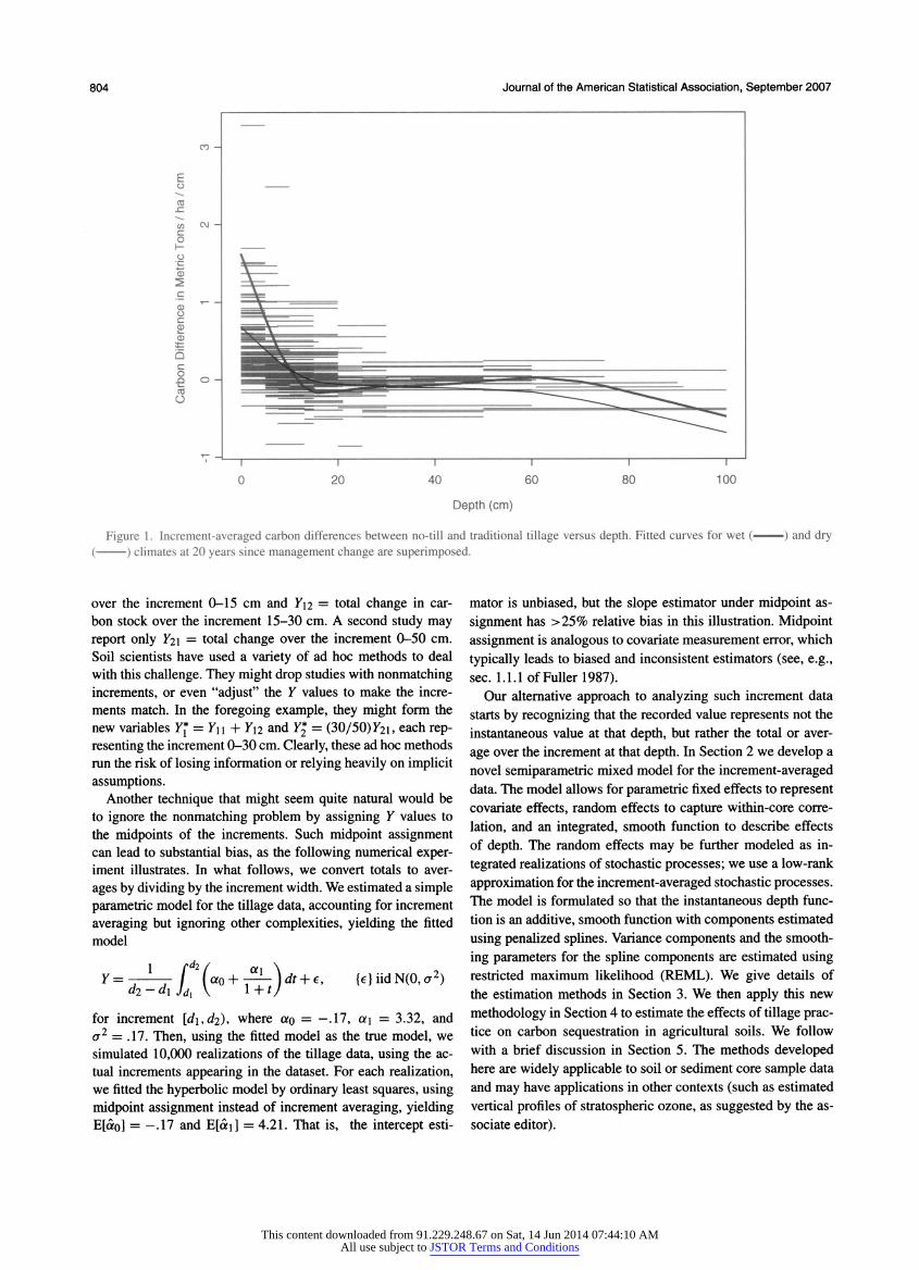
gregated for carbon stock analysis. There are 63 paired studies in these data, with a total of 211 increments. The increment

averaged data are displayed in Figure 1. The upper and lower

endpoints of these increments vary from study to study. For ex

ample, one study may report Y\\ = total change in carbon stock

? 2007 American Statistical Association Journal of the American Statistical Association

September 2007, Vol. 102, No. 479, Applications and Case Studies DOI 10.1198/016214506000001167

803



804 Journal of the American Statistical Association, September 2007

Depth (cm)

Figure 1. Increment-averaged carbon differences between no-till and traditional tillage versus depth. Fitted curves for wet ( ) and dry (??) climates at 20 years since management change are superimposed.

over the increment 0-15 cm and Y12 = total change in car

bon stock over the increment 15-30 cm. A second study may

report only I21 = total change over the increment 0-50 cm.

Soil scientists have used a variety of ad hoc methods to deal with this challenge. They might drop studies with nonmatching increments, or even "adjust" the Y values to make the incre

ments match. In the foregoing example, they might form the new variables Y?

= YU + Y\2 and Y* = (30/50)Y2u each rep

resenting the increment 0-30 cm. Clearly, these ad hoc methods run the risk of losing information or relying heavily on implicit assumptions.

Another technique that might seem quite natural would be to ignore the nonmatching problem by assigning Y values to

the midpoints of the increments. Such midpoint assignment can lead to substantial bias, as the following numerical exper iment illustrates. In what follows, we convert totals to aver

ages by dividing by the increment width. We estimated a simple parametric model for the tillage data, accounting for increment

averaging but ignoring other complexities, yielding the fitted

model

Y = ?[? f2(ao

+ ^A

dt + , { } iid N(0, a2) d2-d\ Jdl V 1+r/

for increment \d\,d2), where oto = ?.17, ai = 3.32, and

a2 = .17. Then, using the fitted model as the true model, we

simulated 10,000 realizations of the tillage data, using the ac

tual increments appearing in the dataset. For each realization, we fitted the hyperbolic model by ordinary least squares, using

midpoint assignment instead of increment averaging, yielding E[ao] = ? 17 and E[?i] = 4.21. That is, the intercept esti

mator is unbiased, but the slope estimator under midpoint as

signment has >25% relative bias in this illustration. Midpoint

assignment is analogous to covariate measurement error, which

typically leads to biased and inconsistent estimators (see, e.g., sec. 1.1.1 of Fuller 1987).

Our alternative approach to analyzing such increment data

starts by recognizing that the recorded value represents not the

instantaneous value at that depth, but rather the total or aver

age over the increment at that depth. In Section 2 we develop a

novel semiparametric mixed model for the increment-averaged data. The model allows for parametric fixed effects to represent covariate effects, random effects to capture within-core corre

lation, and an integrated, smooth function to describe effects

of depth. The random effects may be further modeled as in

tegrated realizations of stochastic processes; we use a low-rank

approximation for the increment-averaged stochastic processes. The model is formulated so that the instantaneous depth func

tion is an additive, smooth function with components estimated

using penalized splines. Variance components and the smooth

ing parameters for the spline components are estimated using restricted maximum likelihood (REML). We give details of

the estimation methods in Section 3. We then apply this new

methodology in Section 4 to estimate the effects of tillage prac tice on carbon sequestration in agricultural soils. We follow

with a brief discussion in Section 5. The methods developed here are widely applicable to soil or sediment core sample data

and may have applications in other contexts (such as estimated

vertical profiles of stratospheric ozone, as suggested by the as

sociate editor).



Breidt, Hsu, and Ogle: Semiparametric Mixed Models 805

2. SEMIPARAMETRIC MIXED MODEL FOR INCREMENT-AVERAGED DATA

2.1 Model Specification

Assume that the sample consists of m independent paired studies and that the ith study has n? increments {[dij-\, dij)}^{, where dij- \ and dy indicate the top and bottom bounds of the

ijth datum. Let F/y denote the increment average in the jth in crement from the ith study, and assume that it satisfies the fol

lowing model:

Yij = xjj? + ??- / g(t; W/) dt + b?u? + iJ9 (1)

dij dij-\ Jdij-i

where ? is a vector of unknown regression coefficients; Xy and

w/ are known covariate vectors; g(t; w/) is a smooth function

of depth, t\ W[ are iid N(0, (J^Ilxl) vectors of random effects; and ij are iid N(0, a2) errors, independent of u/. The vector

by is fixed but may depend on unknown covariance parameters,

as described in Section 2.3. As the notation suggests, w? is a

characteristic of the study that is not increment-specific (e.g.,

soil type, climate factors, and number of years since manage

ment change in our example). Increment-specific effects can be

incorporated without loss of generality in xj-?, rather than in g, where they might violate the assumed smoothness.

The model in (1) is a semiparametric mixed model, similar in spirit to that of Zhang, Lin, Raz, and Sowers (1998); see also the references given by Ruppert, Wand, and Carroll (2003, sec. 9.4). Due to the increment averaging, linear functionals of

g, not g itself, underlie the observations. Engle, Granger, Rice,

and Weiss (1986) considered a similar problem using cross validated smoothing splines (see also Wahba 1990). Our ap proach is based on penalized splines, with penalties selected

automatically using REML. It is easily implemented using stan dard software.

2.2 Integrated Nonparametric Function Specification

Let w/ = (w/i,..., Wiq)7. We assume that g(t; w?) is an addi

tive varying-coefficient model (Hastie and Tibshirani 1993),

q

g(?;w/) = ]Ta?(r)wtf, i=\

where the component smooth functions are allowed to be

splines, although polynomials with lower degrees of freedom are special cases. For these splines, we use the truncated power

basis with a common set of fixed knots, k\ < < kk (although other choices of basis or knots could be easily incorporated),

K

a?(t) = a0i + ant H-h ap?f + ^ aki(t

- Kk)p+, (2)

k=\

where (t)+ = f if t > 0 and 0 otherwise and p is the degree

of the spline. Here the o^'s are fixed, unknown coefficients,

whereas the au are iid N(0, o2?) random effects. If the num

ber of knots K is sufficiently large, then the class of functions

at (t) is very large and can approximate most smooth functions with a high degree of accuracy. For

a2? = co, the splines would

be piecewise polynomials and would require fitting of a large number of parameters. We rule out this case by considering

?ai < ??' m wmcn me spline coefficients au are shrunken to

ward 0, resulting in a smooth yet parsimonious fit. The limiting case of a2g

= 0 is the global pth order polynomial, which is

very smooth. This representation of a smoothing problem as a

mixed model has a long history (see, e.g., Wahba 1978; Robin son 1991; and the extensive references in Ruppert et al. 2003).

The increment average of the additive varying-coefficient model is

l rdv

'ij-dij-i JdiJ_ dh

q

g(t\vfi)dt

?

t2 t?+ otoit + au? H-Ya.pt

P+lJr WH

dij ?

dij-1

?{e^?^-^1-^-?-^1)} i=\ \k=\p )

WU . (3) dij

- dij

Substituting (3) into (1) then yields a linear mixed model for the increment-averaged data.

2.3 Random-Effect Specification

The vectors {u?} capture spatial autocorrelation among incre

ments at different depths from the same study/site. One possible model for the study-specific random effects arises by assuming that they come from an increment-averaged stochastic process,

i rd'j Uij =

-- / Uiit)dt, (4)

i n JiJ= i?a?

dij-dij-i Jdij,

where U?(t) are independent, mean-0, Gaussian stochastic

processes. In the application of this article, these processes can

be interpreted as random differences in carbon profiles between selected no-till and traditional tillage fields; that is, fields are not perfectly paired in the tillage experiments. Assuming no

systematic bias in the assignment of tillage methods to fields, the average random difference should be zero. In effect, this

stochastic process model specifies that the site-specific profile would be a noisy function of depth, g(t, w?) -f Ui(t), but the av

erage over all such profiles (with the same w; covariates) would be the smooth function g(t, wz). This model is full rank in the sense of assuming a complete set of latent, correlated random

variables, one for every observed increment.

For ease of computation, we use instead a low-rank model

(Eilers and Marx 1996; Hastie 1996; Ruppert et al. 2003, secs. 3.12 and 13.4.4), which can be viewed as an approximation to

(4) obtained by projecting the increment-specific random ef fects [Uij]i<j<n? onto a smaller vector of L orthogonal random

? l II variables, uz- = crrjilL u*, where

u7 = fl^iDdr T?-Tg-\ Jl<?<L

?lL =

cov(u*, u*), and 0 = to < t\ < T2 < < r^ are fixed,

known knots. Then the projection of {Uij]\<j<ni onto the space spanned by the components of u; is given by

[Uijh^n^lbJjU,],




where

[bfjUxL^VlJ2 COW([Uij]i<j<n?,Ui).

The bJ-Ui are then substituted into (1). Among the many possible specifications for the stochastic

process U?(t), we focus on two: Ui(t) =

?// is iid N(0, a^), lead

ing to conventional random effects for study (compound sym metry), and Ui(t) is a nonhomogeneous Ornstein-Uhlenbeck

(NOU) process with variance function var(?//(i)) = cr^exp(?0 and correlation function corr(?/z(s), U?(t)) = exp{

? y\s

? t\],

where y > 0. Details of the co vari anee matrices ?l? and B# =

[bill</<?;;i<i<m f?r me increment-averaged NOU process are

given in the Appendix.

3. ESTIMATION

3.1 Estimation of Model Parameters

Let 0 contain all covariance parameters (a2x,..., a2 a^,

a2, as well as ? and y, if present). Set n = XX=i ni and define

y ?

(-Ml > > *\n\ ? ? *ml ? ?

^mnm)ixni

= (^11,

- ..,^lm ?^ral5 ?/ lx/z'

X ? Lxy Jl </'<?/ ;l<Km>

dr = A djj + djj-i " 2

^+i_^+i

(p+l)(d//-*J-i)/ix(p+i)

aJ = (?oi?. ..,api;

. ..;a0i?,... ,<Xpq)\Xq(p+i),

Wi =

[w/id^,..., wiq?jj]i<j<ni.i<i<m

T

dij ?

dij-i

(dtj-Kx)^1 (dij-i -

ki)p+1

p+1

(</(/ -

KK)P+ (dij-i -kk)p+

p+l

W2 = [wnsfj,

..., WiqSfj] !</<?,. ;!</<?

lxtf

a? =

(?i?, ...,aK?),

Be =blockdiag{[b^]i</<W|.}i

Ur = (u[, ...,U^)ixmL,

Q = [X,Wi,W2,B0],

and

Atf =

j?1

0

0

0

0

oC2I/-x? aq

o _o

^?y IftiLxmL.

Then the model (1) for the increment-averaged data can be writ ten as the linear mixed model

y = X/? + Wi<x + W2

af

+ B0U + *. (5)

If the covariance parameters 0 in B# and A# are known, then

the best linear unbiased predictors (BLUPs) of the unknown coefficients and random effects are given by

?

BLUP

a ai

*q u

:(C?C$+cr2 A0rlC?y. (6)

If the covariance parameters are unknown, they can be first

estimated using maximum likelihood or REML, then plugged in to (6) to obtain empirical best linear unbiased predictions (EBLUPs). These analyses, including estimation of variance

parameters o2x,..., a2, Oy, o2 can be implemented using standard software, such as PROC MIXED in SAS or lme() in S-PLUS. (We estimated the covariance parameters ? and y in a

separate optimization, then treated them as fixed in the remain

ing estimation steps.) Numerous practical tips on smoothing with mixed-model software, including code, have been given by Ngo and Wand (2004).

Fitting of the linear mixed model in this way can also be viewed as penalized maximum likelihood with penalties X2 ?

<72<t^ on the sum of squared spline coefficients; therefore, the

fitted splines are penalized splines or P-splines with roughness penalty parameters automatically selected through likelihood based methods. The total degrees of freedom (df) for this fit is

df = trace{C?(C[C? -a2A?r (7)

Degrees of freedom for each component of the fit can be obtained by an appropriate partition of the columns of C? (Hastie and Tibshirani 1990, sec. 3.5; Ruppert et al. 2003, sec. 8.3). For example, the df for the ?th varying coefficient function in git; w) is obtained by defining E? to be the diago nal matrix with l's in the diagonal positions corresponding to

otoe, , otpi,a\i,..., oki, with 0's elsewhere on the diagonal. Then

df? =trace{C?E?(C[C? +a2A?)-1Cp.

3.2 Estimation of the Depth Profile

Now consider estimation of the population-level depth pro file (integrating out study-specific random effects u?) for given covariates xt, w =

(w\,..., wq)T. Define

dj =

il,t,...,tp),

sJ=(it-Kl)P,,...,it-KK)P{_)lxK,

and

cf =

[xj, widj,..., wqdj, sfwi,..., sjwq, 0,..., 0].

Then the EBLUP of the population-level profile at depth t is

given by

EBLUP(xf j8 + git, w)) = cJiC?Ce + ^Aj)"1^. (8)

An approximate pointwise (1 ?

a) 100% confidence band for the population-level profile is then given (at depth t) by

[eq. iS)]?zil-a/2)oJcJiC?Ce+o2A?)-ict, (9)




where z(l ?

a?2) is the (1 ?

a/2) quantile of a standard normal. This confidence band accounts for both variance and squared bias in the fitted depth profile (see Wahba 1983; Nychka 1988;

Ruppert et al. 2003, sec. 6.4).

4. APPLICATION TO CARBON SEQUESTRATION IN AGRICULTURAL SOILS

4.1 Background

We now apply the methodology of the previous sections to the no-till studies described in Section 1. The basic data are the increment averages,

dij ?

dij-\

'

where

NTij ? total carbon stock in

[d/j-i, dy) under no-till,

TTij ? total carbon stock in [<i/j_i, dij)

under traditional tillage,

and the increment average is in units of metric tons of carbon

per hectare per cm. The difference is computed from paired ob servations with and without the management change from tra

ditional tillage to no-till. The difference represents the cumu lative effect over the years since the management change. The

variable years records time since management change, which

varies from 1 to 33 years in these data. Increments vary in width from 2.5 to 60 cm, and vary in depth from the topmost end

point at 0 cm to the bottommost endpoint at 100 cm. Figure 1 illustrates the variability in increment widths and depths. The data also contain two other covariates: an indicator for soil type

(aquic = 1 for aquic soil, 0 otherwise) and an indicator for cli mate condition (wet = 1 for wet climate, 0 otherwise).

We use the truncated linear basis (p = 1) in what follows. We write depth as shorthand for

/ djj + djj-i idij-K\)\- (djj-i -k\)\ \ 2

' dij-dij-i

(djj ~

kk)\ -

jdjj-i -

kk)\ \

dij-dij-i )

in the case with increment averaging, and as shorthand for

(l,r, (t-KX)+,...,it-KK)+)

in the case without increment averaging (i.e., for the population

depth profile). The knots (k\ , /q, , kk)T are chosen to be the

vector of ordered, distinct bottom (right-side) endpoints from the {dij : 1 <j

< wz-; 1 < / < m], yielding K = 21. This choice of knots is somewhat arbitrary, but the bottom endpoints are

convenient and naturally "adaptive" to local depth function cur

vature in a scientifically meaningful way, in the sense that sci

entists have used finer increments near the soil surface, where

they expect to see more tillage effects. Knot choice does not

seem critical in this application, because results with equally spaced knots are nearly identical to those described in this sec

tion.

There are two key inferential goals in this analysis. The first is to estimate the mean function, identifying important fixed ef fects and sources of variation, so that in particular the depth

function g(t; w) can be estimated and examined. This depth function is of scientific interest because it shows the effect of

management change on carbon storage as a function of depth,

time, and other covariates. In other words, it is of interest to

address questions such as, "after 15 years, at what depth is the

effect of conservation tillage evident?" Such questions have po tential implications for agricultural policy, in terms of account

ing for carbon uptake in the soil, particularly for those countries or institutions using agricultural management to mitigate green

house gas emissions.

The second inferential goal is to estimate the total (not aver

age) population-level carbon difference between the two tillage systems over the increment 0-30 cm,

/ 30

IPCC(H)= / {xTH?+g(t,wH)}dt, Jo where x# and w# are the vectors of covariates evaluated at

H years since a management change. The Intergovernmental Panel on Climate Change (IPCC) recommends accounting for

tillage effects in the top 30 cm and over a 20-year time period after management change, because this will presumably cap ture most of the change in organic carbon storage due to man

agement activity (Intergovernmental Panel on Climate Change 1997). These IPCC integrals are critical for comparison to the carbon equivalents of N20 and CH4, the other two key GHGs.

4.2 Model Selection

Model selection was carried out informally by first consid

ering model (1) with random effects Uij ? ?/; and {?//} iid

N(0, Gy). We considered a large number of models with various fixed effects and additive nonparametric functions. Estimates of fixed effects, variance components, and smoothing parame ters were obtained by maximum likelihood (rather than REML) to allow sensible Akaike information criterion (AIC) compu tations. Versions of AIC were then computed using different values of degrees of freedom in the penalty: number of esti

mated hyperparameters (number of columns of [X, Wi] plus number of estimated variance components), df for the complete smoother matrix (fixed effects, spline smooths, and study-level random effects) from (7), and df for the complete smoother mi nus df for study-level random effects.

This preliminary model selection focused attention on non

parametric functions of depth only, with no fixed effects xT?. Exclusion of such fixed effects is a priori reasonable because a fixed effect in this context is an additive constant that changes carbon storage at all depths for all times. Clearly, effects of co

variates, if any, should be greatest near the surface where tillage occurs and should be nearly zero deep in the profile, where

tillage has a negligible impact. This is exactly a covariate by depth interaction. Therefore, we focused on the 24 ? 1 = 15 models that included at least one of the nonparametric terms

depth, aquic*depth, wet*depth, or years*depth. Among these

15 models, the top four (as ranked by any of the AIC val

ues) all contained wet*depth and years*depth, with the best model overall containing only those two terms. Support for

aquic*depth was weak, with two of the top four models ex

cluding this term.

Next, we included a NOU random effect for study as de scribed in Section 2.3, using L = 1 and r\ ? 100. Larger val ues of L were not considered because there are only about




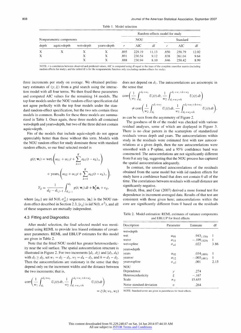
Table 1. Model selection

Random-effects model for study

Nonparametric components NOU Standard

depth aquic*depth wet*depth years *depth r AIC df r AIC df

X X X X .895 229.19 11.13 .850 258.79 12.02 X XX .891 230.54 9.12 .838 261.04 9.64

X X .888 230.94 8.10 .846 258.42 8.99

NOTE: r is correlation between observed and predicted values, AIC is computed using df equal to the trace of the complete smoother matrix (including random effects for study), and the tabled df is for the nonparametric function only (excluding random effects for study).

three increments per study on average. We obtained prelimi

nary estimates of (y, ?) from a grid search using the interac tion model with all four terms. We then fixed these parameters and computed AIC values for the remaining 14 models. The

top four models under the NOU random-effect specification did not agree perfectly with the top four models under the stan dard random-effect specification, but the two sets contain three

models in common. Results for these three models are summa

rized in Table 1. Once again, these three models all contained

wet*depth and years*depth, but two of the three did not contain

aquic*depth. Fits of the models that include aquic*depth do not appear

appreciably better than those without this term. Models with the NOU random effect for study dominate those with standard random effects, so our final selected model is

g(t; Wz) = wet/1 aoi + aut + ^ak\ (t

- Kk)+ I

+ years, I a02 + aut + ^ak2(t

- Kk)+

J,

1 rd'i]

Yij = i--,- / gif\ w/) dt + bju/ + ij, dij-dij-i Jd^

where {ak?} are iid N(0, g2?) sequences, {uz} is the NOU ran

dom effect described in Section 2.3, {?//} is iid N(0, a2), and all of these sequences are mutually independent.

4.3 Fitting and Diagnostics

After model selection, the final selected model was reesti mated using REML to provide less biased estimates of covari ance parameters. REML and EBLUP estimates for this model are given in Table 2.

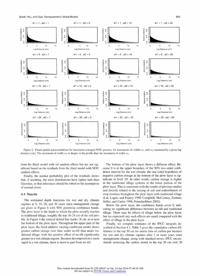
Note that the fitted NOU model has greater heteroscedastic

ity near the soil surface. The spatial autocorrelation structure is

illustrated in Figure 2. For two increments [d\, d2) and [d^, d\) with d^ > d2, set w\ =d2?d\,w2

= d$ ?d?,, and h ? d^? d2.

Then the autocorrelations are stationary in the sense that they

depend only on the increment widths and the distance between the two increments; that is,

(j pd\+w\ y rd\+w\+h+W2 \ ?

/ Ui(t)dt,? / Ui(t)dt) Wl Jdx w2 Jdi+wx+h ) ? ?(h; w\, w2)

does not depend on d\. The autocorrelations are anisotropic in

the sense that

>d\+w\ j pd\+w\+h+W2 corrj

]d\ w2 Jdl+W[+h

? / Uiit)dt,? \ Ui(t)dt) ^1 Jd, W2 Jdx+wx+h )

? / Ui(t)dt,? / ?//(f)df), ^2 Jj, Wi Jdx+W2+h )

as can be seen from the asymmetry of Figure 2.

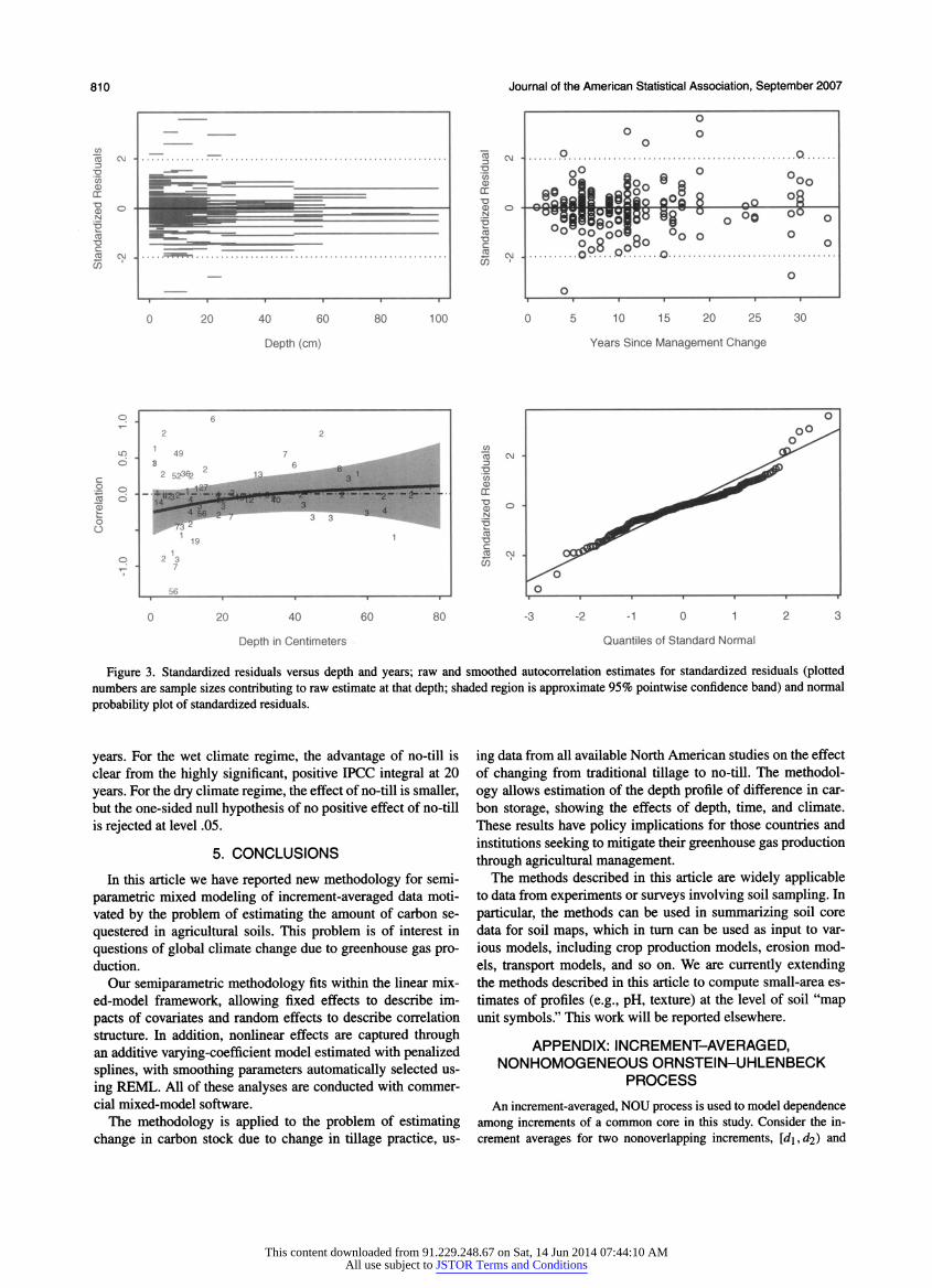
The goodness of fit of the model was checked with various residual analyses, some of which are displayed in Figure 3. There is no clear pattern in the scatterplots of standardized residuals versus depth and years. The autocorrelations within

study in the residuals were estimated first with raw autocor

relations at a given depth, then the raw autocorrelations were

smoothed with a P-spline, and a 95% confidence band was constructed. The autocorrelations are not significantly different

from 0 at any lag, suggesting that the NOU process has captured the spatial autocorrelation adequately.

In contrast, the smoothed autocorrelations of the residuals

obtained from the same model but with iid random effects for

study have a confidence band that does not contain 0 all of the time. The correlations between residuals with small distance are

significantly negative. Breidt, Hsu, and Coar (2007) derived a more formal test for

dependence in increment-averaged data. Results of that test are

consistent with those given here; autocorrelations within the core are significantly different from 0 based on the residuals

Table 2. Model estimation: REML estimates of variance components and EBLUP for fixed effects

Description Parameter Estimate df

wet*depth wet ?oi 943(.156)

1

wet*i a ii ?.109(029) 1

wet*spline o a\ .022 3.86

years* depth

years a02 034(>009) i

years*r a12 --003(.0oi) 1

years*spline oa2 .001 2.15

NOU

Dependence y .21A

Heteroscedasticity ? ?.167

Scale o u 15.655

Noise standard deviation o .264

NOTE: Standard errors are given in parentheses for fixed effects.



Breidt, Hsu, and Ogle: Semiparametric Mixed Models

w1 = 1 , w2 = 1 w1 = 1 , w2 = 5

809

w1 = 1 , w2= 10 w1 = 1 , w2 = 20

0 5 10

Lag Distance (cm)

w1 = 5 , w2 = 1

5 10

Lag Distance (cm)

w1 = 5 , w2 = 5

5 10

Lag Distance (cm)

w1 =5 , w2 = 10

5 10

Lag Distance (cm)

w1 = 5 , w2 = 20

5 10

Lag Distance (cm)

w1 = 10 , w2 = 1

5 10

Lag Distance (cm)

w1 = 10 , w2 = 5

5 10

Lag Distance (cm)

w1 = 10 , w2 = 10

5 10

Lag Distance (cm)

w1 = 10 , w2 = 20

5 10

Lag Distance (cm)

w1 = 20 , w2 = 1

5 10

Lag Distance (cm)

w1 = 20 , w2 = 5

5 10

Lag Distance (cm)

w1 =20 , w2 = 10

5 10

Lag Distance (cm)

w1 = 20 , w2 = 20

5 10

Lag Distance (cm)

5 10

Lag Distance (cm;

5 10

Lag Distance (cm)

5 10

Lag Distance (cm)

Figure 2. Fitted spatial autocorrelations for increment-averaged NOU process, for increments of widths w\ and w2 separated by a given lag distance (cm). The increment of width w2 is deeper in the profile than the increment of width w\.

from the fitted model with iid random effects but are not sig nificant based on the residuals from the fitted model with NOU random effects.

Finally, the normal probability plot of the residuals shows

that, if anything, the error distributions have lighter tails than

Gaussian, so that inferences should be robust to the assumption

of normal errors.

4.4 Results

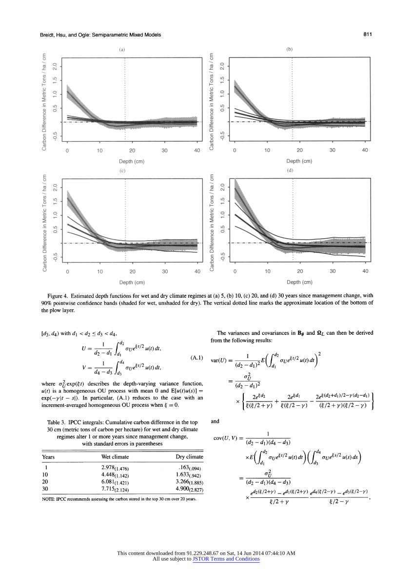
The estimated depth functions for wet and dry climate

regimes at 5, 10, 20, and 30 years since management change are given in Figure 4 with 90% pointwise confidence bands. The plow layer is the depth to which the plow actually reaches in traditional tillage, roughly the top 18-24 cm of the soil pro file. In Figure 4 the vertical dotted line marks 18 cm, at or near

the bottom of the plow layer. Throughout the upper part of the

plow layer, the fitted additive varying-coefficient model shows

greater carbon storage over time under no-till than under tra

ditional tillage, with this positive effect of no-till significantly greater in a wet climate regime. Because decomposition is more

rapid in a wet climate, there is more to gain from no-till.

The bottom of the plow layer shows a different effect. Be cause 0 is at the upper boundary of the 90% two-sided confi dence interval for the wet climate, the one-sided hypothesis of

negative carbon storage at the bottom of the plow layer is sig nificant at level .05. In other words, carbon storage is higher in the traditional tillage systems in the lower portion of the

plow layer. This is consistent with the results of previous studies and directly related to the mixing of soil and redistribution of

crop residues throughout the plow layer with traditional tillage (Lai, Logan, and Fausey 1990; Campbell, McConkey, Zentner, Selles, and Curtin 1996; Franzluebbers 2002).

Below the plow layer, the confidence bands cover 0, indi

cating no significant difference between no-till and traditional

tillage. There may be effects of tillage below the plow layer, but (as expected) any such effects are small compared with the effect of tillage in the plow layer.

Finally, we compute estimates of the IPCC integrals de scribed in Section 4.1. Table 3 gives the cumulative carbon dif ference in the top 30 cm (in metric tons of carbon per hectare) for wet and dry climate regimes after 1 or more years since

management change, along with standard errors. IPCC recom

mends assessing the carbon stored in the top 30 cm over 20




? CM

1

c>J

1

o

o

8? So 8 8 ?oo

.o?. .. o".o.

10 15 20 25

Years Since Management Change

30

?

o ?

20 40 60

Depth in Centimeters

?

-2-10 1

Quantiles of Standard Normal

Figure 3. Standardized residuals versus depth and years; raw and smoothed autocorrelation estimates for standardized residuals (plotted

numbers are sample sizes contributing to raw estimate at that depth; shaded region is approximate 95% pointwise confidence band) and normal

probability plot of standardized residuals.

years. For the wet climate regime, the advantage of no-till is clear from the highly significant, positive IPCC integral at 20

years. For the dry climate regime, the effect of no-till is smaller, but the one-sided null hypothesis of no positive effect of no-till is rejected at level .05.

5. CONCLUSIONS

In this article we have reported new methodology for semi

parametric mixed modeling of increment-averaged data moti vated by the problem of estimating the amount of carbon se

questered in agricultural soils. This problem is of interest in

questions of global climate change due to greenhouse gas pro duction.

Our semiparametric methodology fits within the linear mix ed-model framework, allowing fixed effects to describe im

pacts of covariates and random effects to describe correlation structure. In addition, nonlinear effects are captured through an additive varying-coefficient model estimated with penalized splines, with smoothing parameters automatically selected us

ing REML. All of these analyses are conducted with commer

cial mixed-model software. The methodology is applied to the problem of estimating

change in carbon stock due to change in tillage practice, us

ing data from all available North American studies on the effect of changing from traditional tillage to no-till. The methodol

ogy allows estimation of the depth profile of difference in car

bon storage, showing the effects of depth, time, and climate. These results have policy implications for those countries and

institutions seeking to mitigate their greenhouse gas production through agricultural management.

The methods described in this article are widely applicable to data from experiments or surveys involving soil sampling. In

particular, the methods can be used in summarizing soil core

data for soil maps, which in turn can be used as input to var

ious models, including crop production models, erosion mod

els, transport models, and so on. We are currently extending the methods described in this article to compute small-area es

timates of profiles (e.g., pH, texture) at the level of soil "map unit symbols." This work will be reported elsewhere.

APPENDIX: INCREMENT-AVERAGED, NONHOMOGENEOUSORNSTEIN-UHLENBECK

PROCESS

An increment-averaged, NOU process is used to model dependence

among increments of a common core in this study. Consider the in

crement averages for two nonoverlapping increments, [d\,d2) and




Figure 4. Estimated depth functions for wet and dry climate regimes at (a) 5, (b) 10, (c) 20, and (d) 30 years since management change, with

90% pointwise confidence bands (shaded for wet, unshaded for dry). The vertical dotted line marks the approximate location of the bottom of

the plow layer.

[d$, d^) with d\ <d2<d-$ < ?4,

1 Cdl U =

Ca?

\ oue$t/2u(t)dt,

V=1-^?r ? 4crueW2u(t)dt, dA

- ?3 Jdi

where a^exp(?i)

describes the depth-varying variance function,

u(t) is a homogeneous OU process with mean 0 and E[u(t)u(s)] =

exp(?y\t ?

s\). In particular, (A.l) reduces to the case with an

increment-averaged homogeneous OU process when ? = 0.

Table 3. IPCC integrals: Cumulative carbon difference in the top

30 cm (metric tons of carbon per hectare) for wet and dry climate

regimes alter 1 or more years since management change, with standard errors in parentheses

Years Wet climate Dry climate

1 2-978(1476) .163(094) 10 4.448(1.i42) 1.633(.942) 20 6.081(i.42i) 3.266(L885) 30 7.715(2.i24) 4.900(2.827)

NOTE: IPCC recommends assessing the carbon stored in the top 30 cm over 20 years.

The variances and covariances in B# and f?? can then be derived

from the following results:

var(i/) = \^e( [ 2 orje^2u(t)dt) (d2~d\Y \Jd\ )

~ (d2-dx)2

{2e^d2 2e^ 2?Hd2+d\)/2-y{d2-dx)

*?/2 + y) +

???/2 - Y) "

(?/2 + K)(?/2 - y)

and

1 cov(?/, V) =

(?2-?l)(?4-?3)

x?( / ou^ "

Jd\ J \Jd3 <(( 2ojje^t/2u(t)dt\(? 4oue^2u(s)ds\

7U (d2-dl)(dA-d2>)

ed2il;/2+y) _ed\{%?+y) edA{t-/2-y) _

?d&?-y) X

?/2 + y ?/2-y '




for ? ^ 0. When ? = 0, the foregoing result reduces to the case of an

integrated homogeneous OU process as described following equation

(7) of Sandland and McGilchrist (1979). [Received November 2004.]

REFERENCES Breidt, F. J., Hsu, N. J., and Coar, W. (2007), "A Diagnostic Test for Auto

correlation in Increment-Averaged Data With Application to Soil Sampling," Environmental and Ecological Statistics, to appear.

Campbell, C. A., McConkey, B. G., Zentner, R. P., Seiles, F., and Curtin, D.

(1996), "Tillage and Crop Rotation Effects on Soil Organic C and N in a

Coarse-Textured Typic Haploboroll in Southwestern Saskatchewan," Soil and

Tillage Research, 37, 3-14.

Eilers, P. H. C, and Marx, B. D. (1996), "Flexible Smoothing With B-Splines and Penalties" (with discussion), Statistical Science, 11, 89-121.

Engle, R. F, Granger, C. W. J., Rice, J., and Weiss, A. (1986), "Semiparametric Estimates of the Relation Between Weather and Electricity Sales," Journal of the American Statistical Association, 81, 310-320.

Franzluebbers, A. J. (2002), "Soil Organic Matter Stratification Ratio as an In dicator of Soil Quality," Soil and Tillage Research, 66, 95-106.

Fuller, W. A. (1987), Measurement Error Models, New York: Wiley. Hastie, T. J. (1996), "Pseudosplines," Journal of the Royal Statistical Society,

Ser. B, 58, 379-396.

Hastie, T. J., and Tibshirani, R. J. (1990), Generalized Additive Models, New York: Chapman & Hall.

- (1993), "Varying-Coefficients Models," Journal of the Royal Statisti cal Society, Ser. B, 55, 757-796.

Intergovernmental Panel on Climate Change (1997), Revised 1996 IPCC Guidelines for National Greenhouse Gas Inventories, eds. J. T. Houghton, L. G. Meira Filho, B. Lim, K. Tr?anton, I. Mamaty, Y. Bonduki, D. J. Griggs, and B. A. Callander, Bracknell, U.K.: Intergovernmental Panel on Climate

Change, Meterological Office.

Kern, J. S., and Johnson, M. G. (1993), "Conservation Tillage Impacts on Na tional Soil and Atmospheric Carbon Levels," Soil Science Society of America

Journal, 57, 200-210.

Lai, R., Kimble, J. M., Follett, R. F, and Cole, C. V. (1998), The Potential

of U.S. Cropland to Sequester Carbon and Mitigate the Greenhouse Effect, Chelsea, MI: Sleeping Bear Press.

Lai, R., Logan, T. L, and Fausey, N. R. (1990), "Long-Term Tillage Effects on a

Mollic Ochraqualf in Northwestern Ohio, III: Soil Nutrient Profile," Soil and

Tillage Research, 15, 371-382.

Lindstrom, M. J., Schumacher, T. E., Cogo, N. P., and Blecha, M. L. (1998),

"Tillage Effects on Water Runoff and Soil Erosion After Sod," Journal of Soil and Water Conservation, 53, 59-63.

Ngo, L., and Wand, M. P. (2004), "Smoothing With Mixed-Model Software," Journal of Statistical Software, 9, 1-56.

Nychka, D. W. (1988), "Confidence Intervals for Smoothing Splines," Journal

of the American Statistical Association, 83, 1134-1143.

Paustian, K., Andren, O., Janzen, H. H., Lai, R., Smith, P., Tian, G., Tiessen, H., Van Noordwijk, M., and Woomer, P. L. (1997), "Agricultural Soils as a

Sink to Mitigate CO2 Emissions," Soil Use and Management, 13, 230-244.

Robertson, G. P., Paul, E. A., and Harwood, R. R. (2000), "Greenhouse Gases in Intensive Agriculture: Contributions of Individual Gases to the Radiative

Forcing of the Atmosphere" Science, 289, 1922-1925.

Robinson, G. K. (1991), "That BLUP Is a Good Thing: The Estimation of Ran dom Effects" (with discussion), Statistical Science, 6, 15-51.

Ruppert, D., Wand, M. P., and Carroll, R. J. (2003), Semiparametric Regression, Cambridge, U.K.: Cambridge University Press.

Sandland, R. L., and McGilchrist, C A. (1979), "Stochastic Growth Curve

Analysis," Biometrics, 35, 255-271.

Six, J., Elliott, E. T., Paustian, K., and Doran, J. W. (1998), "Aggregation and Soil Organic Matter Accumulation in Cultivated and Native Grassland Soils," Soil Science Society of America Journal, 62, 1367-1377.

Smith, P., Powlson, D. S., Smith, J. U., Falloon, P., and Coleman, K. (2000),

"Meeting the U.K.'s Climate Change Commitments: Options for Carbon Mit

igation on Agricultural Land," Soil Use and Management, 16, 1-11.

U.S. Department of Agriculture (1994), The USDA Resource Conservation

Systems Applications Program: Designing, Implementing, and Controlling No-Till Systems, Booklet Two, University of Illinois, USDA Soil Con servation Service, Cooperative Extension Service, available at http://www. ag. uiuc. edu/~notill/notill. html.

Wahba, G. (1978), "Improper Priors, Spline Smoothing and the Problem of

Guarding Against Model Errors in Regression," Journal of the Royal Statisti cal Society, Ser. B, 40, 364-372.

- (1983), "Bayesian 'Confidence Intervals' for the Cross-Validated

Smoothing Spline," Journal of the Royal Statistical Society, Ser. B, 45, 133-150.

- (1990), Spline Models for Observational Data, Philadelphia: SIAM.

Zhang, D., Lin, X., Raz, J., and Sowers, M. (1998), "Semiparametric Stochastic Mixed Models for Longitudinal Data," Journal of the American Statistical

Association, 93, 710-7'19.



semiparametric mixed models for increment-averaged data with application to carbon sequestration in...

Documents