This article was downloaded by: [Tufts University]On: 07 October 2014, At: 23:35Publisher: Taylor & FrancisInforma Ltd Registered in England and Wales Registered Number: 1072954 Registeredoffice: Mortimer House, 37-41 Mortimer Street, London W1T 3JH, UK

Journal of Applied StatisticsPublication details, including instructions for authors andsubscription information:http://www.tandfonline.com/loi/cjas20

Semiparametric mixed-effects modelsfor clustered doubly censored dataPao-Sheng Shen aa Department of Statistics , Tunghai University , Taichung ,Taiwan , 40704 , Republic of ChinaPublished online: 10 May 2012.

To cite this article: Pao-Sheng Shen (2012) Semiparametric mixed-effects models forclustered doubly censored data, Journal of Applied Statistics, 39:9, 1881-1892, DOI:10.1080/02664763.2012.684874

To link to this article: http://dx.doi.org/10.1080/02664763.2012.684874

PLEASE SCROLL DOWN FOR ARTICLE

Taylor & Francis makes every effort to ensure the accuracy of all the information (the“Content”) contained in the publications on our platform. However, Taylor & Francis,our agents, and our licensors make no representations or warranties whatsoever as tothe accuracy, completeness, or suitability for any purpose of the Content. Any opinionsand views expressed in this publication are the opinions and views of the authors,and are not the views of or endorsed by Taylor & Francis. The accuracy of the Contentshould not be relied upon and should be independently verified with primary sourcesof information. Taylor and Francis shall not be liable for any losses, actions, claims,proceedings, demands, costs, expenses, damages, and other liabilities whatsoever orhowsoever caused arising directly or indirectly in connection with, in relation to or arisingout of the use of the Content.

This article may be used for research, teaching, and private study purposes. Anysubstantial or systematic reproduction, redistribution, reselling, loan, sub-licensing,systematic supply, or distribution in any form to anyone is expressly forbidden. Terms &Conditions of access and use can be found at http://www.tandfonline.com/page/terms-and-conditions

Journal of Applied StatisticsVol. 39, No. 9, September 2012, 1881–1892

Semiparametric mixed-effects models forclustered doubly censored data

Pao-Sheng Shen∗

Department of Statistics, Tunghai University, Taichung, Taiwan 40704, Republic of China

(Received 30 September 2010; final version received 10 April 2012)

The Cox proportional frailty model with a random effect has been proposed for the analysis of right-censored data which consist of a large number of small clusters of correlated failure time observations.For right-censored data, Cai et al. [3] proposed a class of semiparametric mixed-effects models whichprovides useful alternatives to the Cox model. We demonstrate that the approach of Cai et al. [3] can beused to analyze clustered doubly censored data when both left- and right-censoring variables are alwaysobserved. The asymptotic properties of the proposed estimator are derived. A simulation study is conductedto investigate the performance of the proposed estimator.

Keywords: left censoring; semiparametric transformation model; frailty model

1. Introduction

The Cox regression model [8] has been used extensively, but may not fit the data well. For right-censored data, a well-known class of semiparametric linear transformation models, which includesthe Cox and proportional odds model [1,5,16,19] as special cases, have been studied by Dabrowskaand Doksum [9], Cheng et al. [6,7] and Scharfstein et al. [18]. An important assumption for thevalidity of all these methods is that the failure times are mutually independent. This assumptionis violated if there is some natural or artificial clustering of subjects in the study. Moreover, insurvival or social studies, left censoring and right censoring can occur together naturally and resultin clustered doubly censored data. Consider the following applications.

1.1 Example 1: AIDS clinical trials

A recent AIDS clinical trial was designed to compare the virological responses to different treat-ments for HIV-infected children. One major endpoint of the study was the plasma HIV-1 RNAand HIV-2 RNA levels by the NucliSens assay [2,12]. As a result of the limits of quantification ofthe assay, the observed RNA copies per milliliter of plasma are highly unreliable if above 750,000or below 400. Suppose that we restrict our analysis to subjects who had initial HIV-1 RNA and

∗Email: psshen@thu.edu.tw

ISSN 0266-4763 print/ISSN 1360-0532 online© 2012 Taylor & Francishttp://dx.doi.org/10.1080/02664763.2012.684874http://www.tandfonline.com

Dow

nloa

ded

by [

Tuf

ts U

nive

rsity

] at

23:

35 0

7 O

ctob

er 2

014

1882 P.-S. Shen

HIV-2 RNA levels within the limit of quantification and focus on the change in log10 HIV-k RNA(k = 1, 2) between baseline (week 0) and week 24. For k = 1, 2 and individual i, let lik,s denotethe log10 HIV-k RNA value at week s, and Ti1 = li1,0 − li1,24 and Ti2 = li2,0 − li2,24 denote theresponse variables of the changes at week 24 for HIV-1 RNA and HIV-2 RNA, respectively. LetLik = lik,0 − log10(750000) and Uik = lik,0 − log10(400) be the left-censored and right-censoredvariables, respectively. Then, the response Tik can only be accurately measured within the range[Lik , Uik]. One may be interested in modeling the relationship between Tik and a covariate of vectorZik = [Z1ik , . . . , Zpik]T (e.g. treatment and age). Given i, Ti1 and Ti2 are correlated since they arethe observations from the same infected child i (cluster i).

1.2 Example 2: Follow-up studies

In early childhood learning centers, interest often focuses on testing children to determine whena child learns to accomplish certain tasks [4,15]. Consider a follow-up study for determining theages Tik (i = 1, . . . , n; k = 1, . . . , K) at which the ith child first develops the skill to accomplishtask k (or the brother (k = 1)/sister (k = 2) of the ith brother/sister pair first develops a certaintask). Assume that K is relatively small with respect to n. Let Lik denote the child’s age at entry.Let Uik = min(U1ik , U2ik), where U1ik denotes the child’s age when he or she is lost to follow-upand U2ik denotes the child’s age at the termination of the program. The age Tik can be determinedif the child develops the skill to accomplish task k after he or she is admitted to the program, thatis, Lik ≤ Tik ≤ Uik . However, for some children in the program, the development may have beencompleted before entry, that is, Tik < Lik (left censoring). On the other hand, a right censoringmay occur when a child has not developed the skill by the time of the termination of the program,that is, Uik < Tik . One may be interested in modeling the relationship between Tik and a p × 1vector of covariate Zik = [Z1ik , . . . , Zpik]T (e.g. sex and parents education). Note that given i, Tik’s(k = 1, . . . , K) are correlated since they are the observations from the same child i (cluster i).

For data as described in Examples 1.1 and 1.2, both Lik and Uik are always observed.Thus, we observe a vector (Xik , δik , Lik , Uik , Zik) (i = 1, . . . , n; k = 1, . . . , K), where Xik =min(Uik , max(LiK , Tik)) and δik = 1 if Xik = Tik , δik = 2, if Xik = Uik , and δik = 3, if Xik = Lik .

We assume that given Zik , (Lik , Uik) are independent of Tik . In the following, we confine ourattention to the situation where Zik has a finite number of possible values. This restriction canbe relaxed when (Lik , Uik) are independent of Tik and Zik . Let F(t|Zik) = P(Tik ≤ t|Zik) denotethe cumulative distribution function of Tik given Zik . Similarly, let Q(t|Zik) = P(Uik ≤ t|Zik) andG(t|Zik) = P(Lik ≤ t|Zik) denote the cumulative distribution functions of Uik and Lik given Zik ,respectively. Suppose that the left and right endpoints of Tik , Lik and Uik are independent of Zik .

Let ei denote the unobservable random effect of the ith cluster with the distribution functionLγ (·), where L is a known distribution function with an unknown parameter γ . For clustereddoubly censored data, given ei and Zik , we consider the following mixed-effects transformationmodel:

S(t|Zik , ei) = g{h(t) + βTZik + ei}, (1)

where S(t|Zik , ei) = P(Tik > t|Zik , ei) is the survival function of Tik given Zik , g(·) is a continuous,strictly decreasing link function, h(·) is a completely unspecified strictly increasing function andβ is a p × 1 vector of unknown regression coefficients. Note that when g(·) = exp{− exp(·)},Equation (1) gives the Cox proportional hazard model [8] with frailty exp(ei), and when g(·) =1/(1 + exp(·)), it corresponds to the proportional odds model [1,5,16,19]. Furthermore, note thatmodel (1) has an equivalent form

h(Tik) = −βTZik − ei + εik ,

where the marginal distribution of the error εik is P(εik ≤ x) = F(x) = 1 − g(x).

Dow

nloa

ded

by [

Tuf

ts U

nive

rsity

] at

23:

35 0

7 O

ctob

er 2

014

Journal of Applied Statistics 1883

Let aF = inf{t : F(t|Zik) > 0} and bF = sup{t : F(t|Zik) < 1} denote the left and right end-points of F(·|Zik), and similarly, define (aG, bG) and (aQ, bQ) as the left and right endpointof G(t|Zik), and Q(t|Zik), respectively. Throughout this article, for identifiability of S(t|Zik) =1 − F(t|Zik) for t ∈ (aF , bF), we assume that aG ≤ aF and bF ≤ bQ. Note that this assumption isimportant for obtaining unbiased estimators for β, that is, the right support of the right censoringvariable is larger or equal to that of the underlying failure time and the left support of the leftcensoring variable is shorter than that of the underlying failure time.

For right-censored data, when g(·) is completely specified, Cai et al. [3] proposed a classof estimation procedures for estimating regression parameter β in model (1). In Section 2, wedemonstrate that the approach of Cai et al. [3] can be extended to analyze clustered doublycensored data described in the examples. The asymptotic properties of the proposed estimatorsare derived. In Section 3, simulation studies are conducted to investigate the performance of theproposed estimator.

2. The proposed estimator

In this section, we propose inference procedures for β and γ without estimating the entire infinite-dimensional function h(·). We consider the case where there is no ascertainment bias for selectingclusters or their members in the study, that is, potentially every cluster has K members and the nsets of clustered observations (Tik , Lik , Uik , Zik) are independent and identically distributed. Notethat for k �= l, (Lik , Uik) and (Lil, Uil) are possibly correlated. In practice, individuals in eachcluster may have the same censoring variables (e.g. Example 1.2).

For right-censored data (i.e. Lik ≡ 0), when Uik is independent of covariates and not alwaysobservable, Cai et al. proposed inference procedures based on intra- and inter-cluster comparisonsof failure times. The rank statistics, which quantify such comparisons, are similar to those utilizedby Cheng et al. [6], Fine et al. [10] and Cai et al. [3] for analyzing right-censored data. Here, wedeal with doubly censored data, where censoring variables are always observable and depends oncovariates.

To compare two possible doubly censored observations within the same cluster i, we considerthe quantity

φwilk = I[δik=1]I[Lil≤Xik≤Xil]

W(Xik|Zil, Zik), (2)

where W(x|Zil, Zik) = P(max(Lil, Lik) ≤ x ≤ min(Uil, Uik)|Zil, Zik). Let θ0 = (γ0, βT0 )T be the

true value of θ = (γ , βT)T. Then, conditional on Zil and Zik , we have

E[φwilk] = ζ w

ilk(θ) = E

{E

[I[Til≥Tik ]I[max(Lil ,Lik)≤Tik≤min(Uil ,Uik)]

W(Tik|Zil, Zik)

∣∣∣∣ Tik , Zil, Zik

]}

= E[I[h(Til)≥h(Tik)]|Zil, Zik]

=∫ ∞

−∞

∫ ∞

−∞{1 − F(t + βT

0 Zilk + u)} dF(t + βTZil + u) dLγ0(u), (3)

where Zilk = Zil − Zik . Similarly, to compare two individual observations Xil and Xjk , i �= j, fromdifferent clusters, let

φbijlk = I[δjk=1]I[Lil≤Xjk≤Xil]

W(Xjk|Zil, Zjk). (4)

Dow

nloa

ded

by [

Tuf

ts U

nive

rsity

] at

23:

35 0

7 O

ctob

er 2

014

1884 P.-S. Shen

Then, conditional on Zil and Zjk , we have

E[φbijlk] = ζ b

ijlk(θ) = E

{E

[I[Til≥Tjk ]I[max(Lil ,Ljk)≤Tjk≤min(Uil ,Ujk)]

W(Tjk|Zil, Zjk)

∣∣∣∣ Tjk , Zil, Zjk

]}

= E[I[h(Til)≥h(Tjk)]|Zil, Zjk]

=∫ ∞

−∞

∫ ∞

−∞

∫ ∞

−∞{1 − F(t + βT

0 Zil + u)} dF(t + βT0 Zjk + v) dLγ0(u) dLγ0(v). (5)

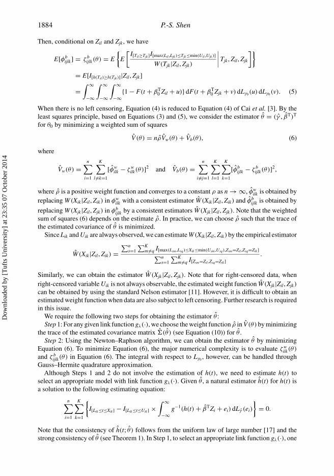
When there is no left censoring, Equation (4) is reduced to Equation (4) of Cai et al. [3]. By theleast squares principle, based on Equations (3) and (5), we consider the estimator θ = (γ , βT)T

for θ0 by minimizing a weighted sum of squares

V(θ) = nρVw(θ) + Vb(θ), (6)

where

Vw(θ) =n∑

i=1

K∑l �=k=1

[φwilk − ζ w

ilk(θ)]2 and Vb(θ) =n∑

i �=j=1

K∑l=1

K∑k=1

[φbijlk − ζ b

ijlk(θ)]2,

where ρ is a positive weight function and converges to a constant ρ as n → ∞, φwilk is obtained by

replacing W(Xik|Zil, Zik) in φwilk with a consistent estimator W(Xik|Zil, Zik) and φb

ijlk is obtained by

replacing W(Xjk|Zil, Zjk) in φbijlk by a consistent estimators W(Xjk|Zil, Zjk). Note that the weighted

sum of squares (6) depends on the estimate ρ. In practice, we can choose ρ such that the trace ofthe estimated covariance of θ is minimized.

Since Lik and Uik are always observed, we can estimate W(Xik|Zil, Zik) by the empirical estimator

W(Xik|Zil, Zik) =∑n

s=1

∑Km �=q I[max(Lsm ,Lsq)≤Xik≤min(Usm ,Usq),Zsm=Zil ,Zsq=Zik ]∑n

s=1

∑Km �=q I[Zsm=Zil ,Zsq=Zik ]

.

Similarly, we can obtain the estimator W(Xjk|Zil, Zjk). Note that for right-censored data, whenright-censored variable Uik is not always observable, the estimated weight function W(Xjk|Zil, Zjk)

can be obtained by using the standard Nelson estimator [11]. However, it is difficult to obtain anestimated weight function when data are also subject to left censoring. Further research is requiredin this issue.

We require the following two steps for obtaining the estimator θ :Step 1: For any given link function gλ(·), we choose the weight function ρ in V(θ) by minimizing

the trace of the estimated covariance matrix �(θ) (see Equation (10)) for θ .Step 2: Using the Newton–Raphson algorithm, we can obtain the estimator θ by minimizing

Equation (6). To minimize Equation (6), the major numerical complexity is to evaluate ζ wilk(θ)

and ζ bijlk(θ) in Equation (6). The integral with respect to Lγ0 , however, can be handled through

Gauss–Hermite quadrature approximation.Although Steps 1 and 2 do not involve the estimation of h(t), we need to estimate h(t) to

select an appropriate model with link function gλ(·). Given θ , a natural estimator h(t) for h(t) isa solution to the following estimating equation:

n∑i=1

K∑k=1

{I[Lik≤t≤Xik ] − I[Lik≤t≤Uik ] ×

∫ ∞

−∞g−1(h(t) + βTZi + ei) dLγ (ei)

}= 0.

Note that the consistency of h(t; θ ) follows from the uniform law of large number [17] and thestrong consistency of θ (see Theorem 1). In Step 1, to select an appropriate link function gλ(·), one

Dow

nloa

ded

by [

Tuf

ts U

nive

rsity

] at

23:

35 0

7 O

ctob

er 2

014

Journal of Applied Statistics 1885

may choose λ by minimizing a quantity which measures the discrepancy between the observedand the fitted value. A reasonable choice of such a measure would be

n∑i=1

K∑k=1

∫ ∞

−∞

{I[Lik≤t≤Xik ] − I[Lik≤t≤Uik ] ×

∫ ∞

−∞g−1

λ (h(t) + βTZi + ei) dLγ (ei)

}2

dv(t), (7)

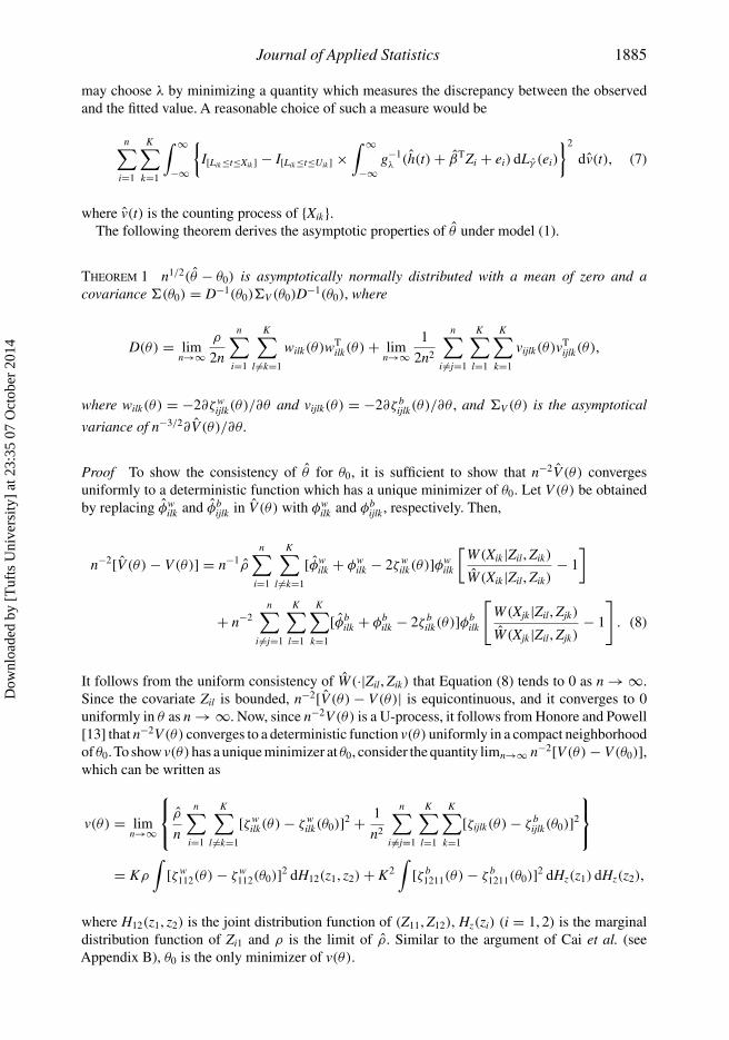
where v(t) is the counting process of {Xik}.The following theorem derives the asymptotic properties of θ under model (1).

Theorem 1 n1/2(θ − θ0) is asymptotically normally distributed with a mean of zero and acovariance �(θ0) = D−1(θ0)�V (θ0)D−1(θ0), where

D(θ) = limn→∞

ρ

2n

n∑i=1

K∑l �=k=1

wilk(θ)wTilk(θ) + lim

n→∞1

2n2

n∑i �=j=1

K∑l=1

K∑k=1

vijlk(θ)vTijlk(θ),

where wilk(θ) = −2∂ζ wijlk(θ)/∂θ and vijlk(θ) = −2∂ζ b

ijlk(θ)/∂θ , and �V (θ) is the asymptotical

variance of n−3/2∂V(θ)/∂θ .

Proof To show the consistency of θ for θ0, it is sufficient to show that n−2V(θ) convergesuniformly to a deterministic function which has a unique minimizer of θ0. Let V(θ) be obtainedby replacing φw

ilk and φbijlk in V(θ) with φw

ilk and φbijlk , respectively. Then,

n−2[V(θ) − V(θ)] = n−1ρ

n∑i=1

K∑l �=k=1

[φwilk + φw

ilk − 2ζ wilk(θ)]φw

ilk

[W(Xik|Zil, Zik)

W(Xik|Zil, Zik)− 1

]

+ n−2n∑

i �=j=1

K∑l=1

K∑k=1

[φbilk + φb

ilk − 2ζ bilk(θ)]φb

ilk

[W(Xjk|Zil, Zjk)

W(Xjk|Zil, Zjk)− 1

]. (8)

It follows from the uniform consistency of W(·|Zil, Zik) that Equation (8) tends to 0 as n → ∞.Since the covariate Zil is bounded, n−2[V(θ) − V(θ)| is equicontinuous, and it converges to 0uniformly in θ as n → ∞. Now, since n−2V(θ) is a U-process, it follows from Honore and Powell[13] that n−2V(θ) converges to a deterministic function v(θ) uniformly in a compact neighborhoodof θ0. To show v(θ)has a unique minimizer at θ0, consider the quantity limn→∞ n−2[V(θ) − V(θ0)],which can be written as

v(θ) = limn→∞

⎧⎨⎩ ρ

n

n∑i=1

K∑l �=k=1

[ζ wilk(θ) − ζ w

ilk(θ0)]2 + 1

n2

n∑i �=j=1

K∑l=1

K∑k=1

[ζijlk(θ) − ζ bijlk(θ0)]2

⎫⎬⎭

= Kρ

∫[ζ w

112(θ) − ζ w112(θ0)]2 dH12(z1, z2) + K2

∫[ζ b

1211(θ) − ζ b1211(θ0)]2 dHz(z1) dHz(z2),

where H12(z1, z2) is the joint distribution function of (Z11, Z12), Hz(zi) (i = 1, 2) is the marginaldistribution function of Zi1 and ρ is the limit of ρ. Similar to the argument of Cai et al. (seeAppendix B), θ0 is the only minimizer of v(θ).

Dow

nloa

ded

by [

Tuf

ts U

nive

rsity

] at

23:

35 0

7 O

ctob

er 2

014

1886 P.-S. Shen

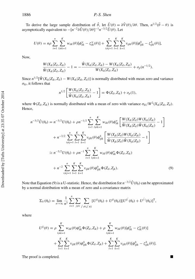
To derive the large sample distribution of θ , let U(θ) = ∂V(θ)/∂θ . Then, n1/2(θ − θ) isasymptotically equivalent to −[n−2∂U(θ)/∂θ ]−1n−3/2U(θ). Let

U(θ) = nρ

n∑i=1

K∑l �=k=1

wilk(θ)[φwilk − ζ w

ilk(θ)] +n∑

i �=j=1

K∑l=1

K∑k=1

vijlk(θ)[φbijlk − ζ b

ijlk(θ)],

Now,

W(Xik|Zil, Zik)

W(Xik|Zil, Zik)− 1 = −W(Xik|Zil, Zik) − W(Xik|Zil, Zik)

W(Xik|Zil, Zik)+ op(n

−1/2).

Since n1/2[W(Xik|Zik , Zil) − W(Xik|Zik , Zil)] is normally distributed with mean zero and varianceσkl, it follows that

n1/2

[W(Xik|Zil, Zik)

W(Xik|Zil, Zik)− 1

]= �(Zil, Zik) + op(1),

where �(Zil, Zik) is normally distributed with a mean of zero with variance σkl/W2(Xik|Zik , Zil).Hence,

n−3/2U(θ0) = n−3/2U(θ0) + ρn−1/2n∑

i=1

K∑l �=k=1

wilk(θ)φwilk

[W(Xik|Zil)W(Xik|Zik)

W(Xik|Zil)W(Xik|Zik)− 1

]

+ n−3/2n∑

i �=j=1

K∑l=1

K∑k=1

vijlk(θ)φbijlk

[W(Xjk|Zil)W(Xjk|Zjk)

W(Xjk|Zil)W(Xjk|Zjk)− 1

]

n−3/2U(θ0) + ρn−1n∑

i=1

K∑l �=k=1

wilk(θ)φwilk�(Zil, Zik)

+ n−2n∑

i �=j=1

K∑l=1

K∑k=1

vijlk(θ)φbijlk�(Zil, Zjk). (9)

Note that Equation (9) is a U-statistic. Hence, the distribution for n−3/2U(θ0) can be approximatedby a normal distribution with a mean of zero and a covariance matrix

�V (θ0) = limn→∞

1

n3

n∑i=1

∑j �=i

∑j′ �=i,j′ �=j

[Uij(θ0) + Uji(θ0)][Uij′(θ0) + Uj

′i(θ0)]T,

where

Uij(θ) = ρ

K∑l �=k=1

wilk(θ)φwilk�(Zil, Zik) + ρ

K∑l �=k=1

wilk(θ)[φwilk − ζ w

ilk(θ)]

+K∑

l=1

K∑k=1

vijlk(θ)φbijlk�(Zil, Zjk) +

K∑l=1

K∑k=1

vijlk(θ)[φbijlk − ζ b

ijlk(θ)].

The proof is completed. �

Dow

nloa

ded

by [

Tuf

ts U

nive

rsity

] at

23:

35 0

7 O

ctob

er 2

014

Journal of Applied Statistics 1887

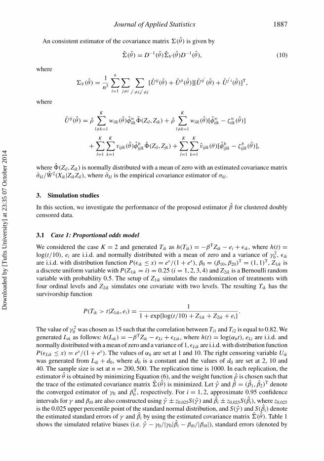
An consistent estimator of the covariance matrix �(θ) is given by

�(θ) = D−1(θ)�V (θ)D−1(θ), (10)

where

�V (θ) = 1

n3

n∑i=1

∑j �=i

∑j′ �=i,j′ �=j

[Uij(θ) + Uji(θ)][Uij′(θ) + Uj

′i(θ)]T,

where

Uij(θ) = ρ

K∑l �=k=1

wilk(θ)φwilk�(Zil, Zik) + ρ

K∑l �=k=1

wilk(θ)[φwilk − ζ w

ilk(θ)]

+K∑

l=1

K∑k=1

vijlk(θ)φbijlk�(Zil, Zjk) +

K∑l=1

K∑k=1

vijlk(θ)[φbijlk − ζ b

ijlk(θ)],

where �(Zil, Zik) is normally distributed with a mean of zero with an estimated covariance matrixσkl/W2(Xik|ZikZil), where σkl is the empirical covariance estimator of σkl.

3. Simulation studies

In this section, we investigate the performance of the proposed estimator β for clustered doublycensored data.

3.1 Case 1: Proportional odds model

We considered the case K = 2 and generated Tik as h(Tik) = −βTZik − ei + εik , where h(t) =log(t/10), ei are i.i.d. and normally distributed with a mean of zero and a variance of γ 2

0 , εik

are i.i.d. with distribution function P(εik ≤ x) = ex/(1 + ex), β0 = (β10, β20)T = (1, 1)T, Z1ik is

a discrete uniform variable with P(Z1ik = i) = 0.25 (i = 1, 2, 3, 4) and Z2ik is a Bernoulli randomvariable with probability 0.5. The setup of Z1ik simulates the randomization of treatments withfour ordinal levels and Z2ik simulates one covariate with two levels. The resulting Tik has thesurvivorship function

P(Tik > t|Z1ik , ei) = 1

1 + exp{log(t/10) + Z1ik + Z2ik + ei} .

The value of γ 20 was chosen as 15 such that the correlation between Ti1 and Ti2 is equal to 0.82. We

generated Lik as follows: h(Lik) = −βTZik − eLi + εLik , where h(t) = log(αht), eLi are i.i.d. andnormally distributed with a mean of zero and a variance of 1, εLik are i.i.d. with distribution functionP(εLik ≤ x) = ex/(1 + ex). The values of αh are set at 1 and 10. The right censoring variable Uik

was generated from Lik + d0, where d0 is a constant and the values of d0 are set at 2, 10 and40. The sample size is set at n = 200, 500. The replication time is 1000. In each replication, theestimator θ is obtained by minimizing Equation (6), and the weight function ρ is chosen such thatthe trace of the estimated covariance matrix �(θ) is minimized. Let γ and β = (β1, β2)

T denotethe converged estimator of γ0 and βT

0 , respectively. For i = 1, 2, approximate 0.95 confidenceintervals for γ and βi0 are also constructed using γ ± z0.025S(γ ) and βi ± z0.025S(βi), where z0.025

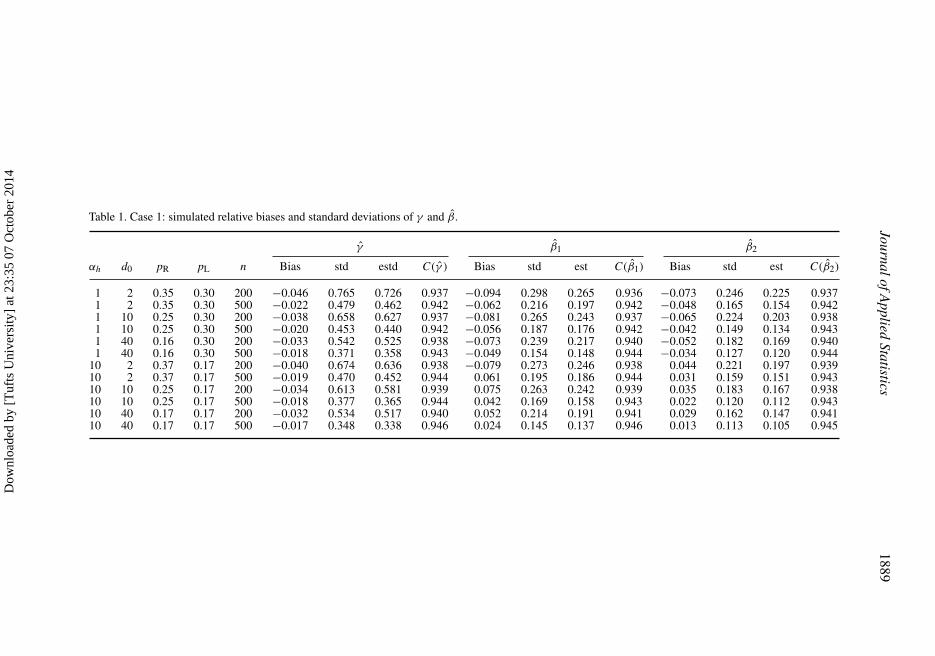
is the 0.025 upper percentile point of the standard normal distribution, and S(γ ) and S(βi) denotethe estimated standard errors of γ and βi by using the estimated covariance matrix �(θ). Table 1shows the simulated relative biases (i.e. γ − γ0/|γ0|βi − βi0/|βi0|), standard errors (denoted by

Dow

nloa

ded

by [

Tuf

ts U

nive

rsity

] at

23:

35 0

7 O

ctob

er 2

014

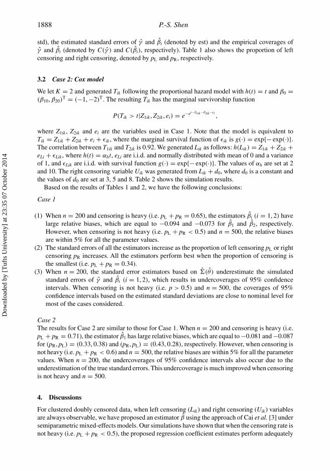
1888 P.-S. Shen

std), the estimated standard errors of γ and βi (denoted by est) and the empirical coverages ofγ and βi (denoted by C(γ ) and C(βi), respectively). Table 1 also shows the proportion of leftcensoring and right censoring, denoted by pL and pR, respectively.

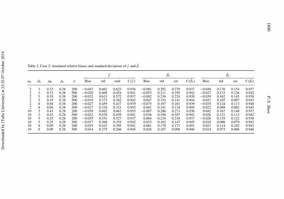
3.2 Case 2: Cox model

We let K = 2 and generated Tik following the proportional hazard model with h(t) = t and β0 =(β10, β20)

T = (−1, −2)T. The resulting Tik has the marginal survivorship function

P(Tik > t|Z1ik , Z2ik , ei) = e−et−Z1ik −Z2ik −ei ,

where Z1ik , Z2ik and ei are the variables used in Case 1. Note that the model is equivalent toTik = Z1ik + Z2ik + ei + εik , where the marginal survival function of εik is g(·) = exp{− exp(·)}.The correlation between T1ik and T2ik is 0.92. We generated Lik as follows: h(Lik) = Z1ik + Z2ik +eLi + εLik , where h(t) = αht, eLi are i.i.d. and normally distributed with mean of 0 and a varianceof 1, and εLik are i.i.d. with survival function g(·) = exp{− exp(·)}. The values of αh are set at 2and 10. The right censoring variable Uik was generated from Lik + d0, where d0 is a constant andthe values of d0 are set at 3, 5 and 8. Table 2 shows the simulation results.

Based on the results of Tables 1 and 2, we have the following conclusions:

Case 1

(1) When n = 200 and censoring is heavy (i.e. pL + pR = 0.65), the estimators βi (i = 1, 2) havelarge relative biases, which are equal to −0.094 and −0.073 for β1 and β2, respectively.However, when censoring is not heavy (i.e. pL + pR < 0.5) and n = 500, the relative biasesare within 5% for all the parameter values.

(2) The standard errors of all the estimators increase as the proportion of left censoring pL or rightcensoring pR increases. All the estimators perform best when the proportion of censoring isthe smallest (i.e. pL + pR = 0.34).

(3) When n = 200, the standard error estimators based on �(θ) underestimate the simulatedstandard errors of γ and βi (i = 1, 2), which results in undercoverages of 95% confidenceintervals. When censoring is not heavy (i.e. p > 0.5) and n = 500, the coverages of 95%confidence intervals based on the estimated standard deviations are close to nominal level formost of the cases considered.

Case 2The results for Case 2 are similar to those for Case 1. When n = 200 and censoring is heavy (i.e.pL + pR = 0.71), the estimator β1 has large relative biases, which are equal to −0.081 and −0.087for (pR, pL) = (0.33, 0.38) and (pR, pL) = (0.43, 0.28), respectively. However, when censoring isnot heavy (i.e. pL + pR < 0.6) and n = 500, the relative biases are within 5% for all the parametervalues. When n = 200, the undercoverages of 95% confidence intervals also occur due to theunderestimation of the true standard errors. This undercoverage is much improved when censoringis not heavy and n = 500.

4. Discussions

For clustered doubly censored data, when left censoring (Lik) and right censoring (Uik) variablesare always observable, we have proposed an estimator β using the approach of Cai et al. [3] undersemiparametric mixed-effects models. Our simulations have shown that when the censoring rate isnot heavy (i.e. pL + pR < 0.5), the proposed regression coefficient estimates perform adequately

Dow

nloa

ded

by [

Tuf

ts U

nive

rsity

] at

23:

35 0

7 O

ctob

er 2

014

JournalofApplied

Statistics1889

Table 1. Case 1: simulated relative biases and standard deviations of γ and β.

γ β1 β2

αh d0 pR pL n Bias std estd C(γ ) Bias std est C(β1) Bias std est C(β2)

1 2 0.35 0.30 200 −0.046 0.765 0.726 0.937 −0.094 0.298 0.265 0.936 −0.073 0.246 0.225 0.9371 2 0.35 0.30 500 −0.022 0.479 0.462 0.942 −0.062 0.216 0.197 0.942 −0.048 0.165 0.154 0.9421 10 0.25 0.30 200 −0.038 0.658 0.627 0.937 −0.081 0.265 0.243 0.937 −0.065 0.224 0.203 0.9381 10 0.25 0.30 500 −0.020 0.453 0.440 0.942 −0.056 0.187 0.176 0.942 −0.042 0.149 0.134 0.9431 40 0.16 0.30 200 −0.033 0.542 0.525 0.938 −0.073 0.239 0.217 0.940 −0.052 0.182 0.169 0.9401 40 0.16 0.30 500 −0.018 0.371 0.358 0.943 −0.049 0.154 0.148 0.944 −0.034 0.127 0.120 0.944

10 2 0.37 0.17 200 −0.040 0.674 0.636 0.938 −0.079 0.273 0.246 0.938 0.044 0.221 0.197 0.93910 2 0.37 0.17 500 −0.019 0.470 0.452 0.944 0.061 0.195 0.186 0.944 0.031 0.159 0.151 0.94310 10 0.25 0.17 200 −0.034 0.613 0.581 0.939 0.075 0.263 0.242 0.939 0.035 0.183 0.167 0.93810 10 0.25 0.17 500 −0.018 0.377 0.365 0.944 0.042 0.169 0.158 0.943 0.022 0.120 0.112 0.94310 40 0.17 0.17 200 −0.032 0.534 0.517 0.940 0.052 0.214 0.191 0.941 0.029 0.162 0.147 0.94110 40 0.17 0.17 500 −0.017 0.348 0.338 0.946 0.024 0.145 0.137 0.946 0.013 0.113 0.105 0.945

Dow

nloa

ded

by [

Tuf

ts U

nive

rsity

] at

23:

35 0

7 O

ctob

er 2

014

1890P.-S.Shen

Table 2. Case 2: simulated relative biases and standard deviations of γ and β.

γ β1 β2

αh d0 pR pL n Bias std estd C(γ ) Bias std est C(β1) Bias std est C(β2)

2 3 0.33 0.38 200 −0.042 0.662 0.623 0.936 −0.081 0.292 0.279 0.937 −0.040 0.176 0.154 0.9372 3 0.33 0.38 500 −0.020 0.468 0.454 0.941 −0.053 0.211 0.195 0.942 −0.027 0.133 0.126 0.9422 5 0.19 0.38 200 −0.032 0.613 0.572 0.937 −0.082 0.236 0.224 0.938 −0.039 0.162 0.145 0.9382 5 0.19 0.38 500 −0.019 0.375 0.362 0.942 0.047 0.154 0.141 0.944 0.031 0.105 0.097 0.9432 8 0.04 0.38 200 −0.027 0.459 0.437 0.939 −0.075 0.197 0.181 0.939 −0.035 0.124 0.113 0.9402 8 0.04 0.38 500 −0.017 0.334 0.321 0.943 0.041 0.141 0.134 0.945 0.022 0.089 0.082 0.945

10 3 0.43 0.28 200 −0.039 0.692 0.663 0.935 −0.087 0.286 0.273 0.936 0.042 0.167 0.148 0.93710 3 0.43 0.28 500 −0.022 0.476 0.459 0.941 0.036 0.198 0.187 0.942 0.026 0.121 0.113 0.94210 5 0.25 0.28 200 −0.035 0.551 0.527 0.937 0.064 0.234 0.218 0.937 −0.026 0.135 0.122 0.93810 5 0.25 0.28 500 −0.017 0.368 0.354 0.942 0.033 0.162 0.147 0.945 0.018 0.086 0.079 0.94310 8 0.09 0.28 200 0.019 0.415 0.395 0.941 0.061 0.178 0.171 0.941 0.023 0.114 0.102 0.94210 8 0.09 0.28 500 0.014 0.275 0.266 0.945 0.026 0.107 0.098 0.946 0.014 0.073 0.068 0.946

Dow

nloa

ded

by [

Tuf

ts U

nive

rsity

] at

23:

35 0

7 O

ctob

er 2

014

Journal of Applied Statistics 1891

with a sample of moderate size (n = 200). However, when the censoring rate is heavy (e.g.pL + pR > 0.6), the relative biases of the proposed regression coefficient estimates can be large.In this case, a large sample size is needed to obtain a reliable estimator. Our simulation studyindicates that when n = 500, the proposed estimator performs well for all the cases considered,where the relative biases are within 6.2% for all the parameter values.

The restriction that Zik is discrete can be relaxed when (Lik , Uik) are independent of Zik . In thiscase, we can replace the estimator W(Xik|Zil, Zik) by a common empirical estimator, say W(Xik)

of P(max(Lil, Lik) ≤ x ≤ min(Uil, Uik)) based on all the observations. Although the proposedestimator in this article requires both the left censoring time and right censoring time are alwaysobservable, it is still practically useful in analyzing the data as described in Examples 1.1 and 1.2.As far as we know, there is no existing alternative estimator. Recently, for clustered right-censoreddata, Zeng et al. [20] considered maximum-likelihood estimation in the transformation model withrandom effects for clustered data. Their likelihood estimator does not require either the covariateto be discrete or the censoring time to be independent of the covariates. However, it is not easy toextend their approach to clustered doubly censored data due to the infinite dimension of h(t). Oneneeds to restrict the jump points of h(t) to some subset of the observations, which may include left-censored points. It requires further research in this issue. Although for clustered right-censoreddata a software package [14] can be used for obtaining the proposed estimators under the Coxmodel, software implementation is not available for doubly censored data.

Acknowledgements

The author thanks the associate editor and referees for their helpful and valuable comments and suggestions.

References

[1] S. Bennett, Analysis of survival data by the proportional odds model, Stat. Med. 2 (1983), pp. 273–277.[2] T. Cai and S. Cheng, Semiparametric regression analysis for doubly censored data, Biometrika 91 (2004), pp. 277–

290.[3] T. Cai, S.C. Cheng, and L.J. Wei, Semiparametric mixed-effect models for clustered failure time data, J. Am. Statist.

Assoc. 97 (2002), pp. 514–522.[4] M.N. Chang and G.L. Yang, Strong consistency of a nonparametric estimator of the survival function with doubly

censored data, Ann. Stat. 15 (1987), pp. 1536–1547.[5] K. Chen, Z. Jin, and Z. Ying, Semiparametric analysis of transformation models with censored data, Biometrika 89

(2002), pp. 659–668.[6] S.C. Cheng, L.J. Wei, and Z. Ying, Analysis of transformation models with censored data, Biometrika 82 (1995),

pp. 835–845.[7] S.C. Cheng, L.J. Wei, and Z. Ying, Prediction of survival probabilities with semi-parametric transformation model,

J. Am. Statist. Assoc. 92 (1997), pp. 277–235.[8] D. Cox, Regression models and life tables (with Discussion), J. R. Statist. Soc. B 34 (1972), pp. 187–220.[9] D. Dabrowska and K. Doksum, Partial likelihood in transformation models with censored data, Scand. J. Statist. 15

(1988), pp. 1–23.[10] J.P. Fine, Z. Ying, and L.J. Wei, On the linear transformation model for censored data, Biometrika 85 (1998),

pp. 980–986.[11] T.R. Fleming and D.P. Harrington, Counting Processes and Survival Analysis, Wiley, New York, 1991.[12] S.G. Geoffrey, E.H. Stephen, D.A. Habibatou, E.S. Joshua, W.C. Cathy, B.K. Nancy, and S.S. Papa, Lower levels of

HIV RNA in semen in HIV-2 compared with HIV-1 infection: Implications for differences in transmission, AIDS 20(2006), pp. 895–900.

[13] B.E. Honore and J.L. Powell, Pairwise difference estimators of censored and truncated regression models, J. Econom.64 (1994), pp. 241–278.

[14] P.J. Kelly, A review of software packages for analyzing correlated survival data, Am. Stat. 58 (2004), pp. 337–342.[15] P.H. Leiderman, D. Babu, J. Kagia, H.C. Kraemer, and G.F. Leiderman, African infant precocity and some social

influences during the first year, Nature 242 (1973), pp. 247–249.

Dow

nloa

ded

by [

Tuf

ts U

nive

rsity

] at

23:

35 0

7 O

ctob

er 2

014

1892 P.-S. Shen

[16] S.A. Murphy, A.J. Rossini, and A.W. van der Vaart, Maximum likelihood estimation in the proportional odds model,J. Am. Statist. Assoc. 92 (1996), pp. 968–976.

[17] D. Pollard, Empirical Processes: Theory and Applications, Institute of Mathematical Statistics, Hayward, CA, 1990.[18] D.O. Scharfstein, A.A. Tsiatis, and P. Gilbert, Semiparametric efficient estimation in the generalized odds-rate class

of regression model for right-censored time to event data, Lifetime Data Anal. 4 (1998), pp. 355–391.[19] S. Yang and R. Prentice, Semiparametric inference in the proportional odds regression model, J. Am. Statist. Assoc.

92 (1999), pp. 968–976.[20] D. Zeng, D.Y. Lin, and X. Lin, Semiparametric transformation modes with random effects for clustered data, Statist.

Sinica 18 (2008), pp. 355–377.

Dow

nloa

ded

by [

Tuf

ts U

nive

rsity

] at

23:

35 0

7 O

ctob

er 2

014