semiparametric bayesian hierarchical models for heterogeneous population in nonlinear mixed effect...
TRANSCRIPT
This article was downloaded by: [The University of British Columbia]On: 11 October 2014, At: 02:53Publisher: Taylor & FrancisInforma Ltd Registered in England and Wales Registered Number: 1072954 Registeredoffice: Mortimer House, 37-41 Mortimer Street, London W1T 3JH, UK
Journal of Applied StatisticsPublication details, including instructions for authors andsubscription information:http://www.tandfonline.com/loi/cjas20
Semiparametric Bayesian hierarchicalmodels for heterogeneous populationin nonlinear mixed effect model:application to gastric emptying studiesHuaiye Zhanga, Inyoung Kima & Chun Gun Parkb
a Department of Statistics, Virginia Polytechnic Institute and StateUniversity, Blacksburg, VA 24061, USAb Department of Mathematics, Kyonggi University, Suwan,Republic of KoreaPublished online: 17 Jun 2014.
To cite this article: Huaiye Zhang, Inyoung Kim & Chun Gun Park (2014) SemiparametricBayesian hierarchical models for heterogeneous population in nonlinear mixed effect model:application to gastric emptying studies, Journal of Applied Statistics, 41:12, 2743-2760, DOI:10.1080/02664763.2014.928848
To link to this article: http://dx.doi.org/10.1080/02664763.2014.928848
PLEASE SCROLL DOWN FOR ARTICLE
Taylor & Francis makes every effort to ensure the accuracy of all the information (the“Content”) contained in the publications on our platform. However, Taylor & Francis,our agents, and our licensors make no representations or warranties whatsoever as tothe accuracy, completeness, or suitability for any purpose of the Content. Any opinionsand views expressed in this publication are the opinions and views of the authors,and are not the views of or endorsed by Taylor & Francis. The accuracy of the Contentshould not be relied upon and should be independently verified with primary sourcesof information. Taylor and Francis shall not be liable for any losses, actions, claims,proceedings, demands, costs, expenses, damages, and other liabilities whatsoever orhowsoever caused arising directly or indirectly in connection with, in relation to or arisingout of the use of the Content.
This article may be used for research, teaching, and private study purposes. Anysubstantial or systematic reproduction, redistribution, reselling, loan, sub-licensing,systematic supply, or distribution in any form to anyone is expressly forbidden. Terms &

Conditions of access and use can be found at http://www.tandfonline.com/page/terms-and-conditions
Dow
nloa
ded
by [
The
Uni
vers
ity o
f B
ritis
h C
olum
bia]
at 0
2:53
11
Oct
ober
201
4
Journal of Applied Statistics, 2014Vol. 41, No. 12, 2743–2760, http://dx.doi.org/10.1080/02664763.2014.928848
Semiparametric Bayesian hierarchicalmodels for heterogeneous population in
nonlinear mixed effect model: application togastric emptying studies
Huaiye Zhanga, Inyoung Kima∗ and Chun Gun Parkb
aDepartment of Statistics, Virginia Polytechnic Institute and State University, Blacksburg, VA 24061, USA;bDepartment of Mathematics, Kyonggi University, Suwan, Republic of Korea
(Received 16 July 2013; accepted 25 May 2014)
Gastric emptying studies are frequently used in medical research, both human and animal, when eval-uating the effectiveness and determining the unintended side-effects of new and existing medications,diets, and procedures or interventions. It is essential that gastric emptying data be appropriately summa-rized before making comparisons between study groups of interest and to allow study the comparisons.Since gastric emptying data have a nonlinear emptying curve and are longitudinal data, nonlinear mixedeffect (NLME) models can accommodate both the variation among measurements within individualsand the individual-to-individual variation. However, the NLME model requires strong assumptions thatare often not satisfied in real applications that involve a relatively small number of subjects, have het-erogeneous measurement errors, or have large variation among subjects. Therefore, we propose threesemiparametric Bayesian NLMEs constructed with Dirichlet process priors, which automatically clus-ter sub-populations and estimate heterogeneous measurement errors. To compare three semiparametricmodels with the parametric model we propose a penalized posterior Bayes factor. We compare the per-formance of our semiparametric hierarchical Bayesian approaches with that of the parametric Bayesianhierarchical approach. Simulation results suggest that our semiparametric approaches are more robust andflexible. Our gastric emptying studies from equine medicine are used to demonstrate the advantage of ourapproaches.
Keywords: Dirichlet process; hierarchical model; nonlinear mixed effect model; semiparametricBayesian
1. Introduction
The main goal of collecting gastric emptying data from humans or animals is to evaluate theeffectiveness and determine the unintended side-effects of new and existing medications, diets,
∗Corresponding author. Email: [email protected]
c© 2014 Taylor & Francis
Dow
nloa
ded
by [
The
Uni
vers
ity o
f B
ritis
h C
olum
bia]
at 0
2:53
11
Oct
ober
201
4
2744 H. Zhang et al.
and procedures or interventions [2,15,28]. It is essential that gastric emptying data be appropri-ately summarized to allow easier comparison between treatments or diets. For the analysis ofthe data from gastric emptying studies, several nonlinear models have been proposed based onexponential, double exponential, power exponential, and modified power exponential functions.The power exponential model is the most popular model for analysing gastric emptying data[9,10]. However, the power exponential model is used for summarizing the gastric emptying foran individual subject, not using all of the observations from other subjects. Summarizing gastricemptying data using all subjects provides more statistical power and is particularly useful for therelatively common studies where there are a relatively small number of subjects. Therefore, weconsider a nonlinear mixed effect (NLME) model in order to accommodate both variation amongmeasurements within individuals and individual-to-individual variation. We further consider thatthe semiparametric NLME model allows to automatically cluster heterogeneous sub-populationsas well as estimate heterogeneous measurement errors.
The NLME model can be fitted using several approaches such as a global two-stage method[7,21,27], an Expectation Maximization algorithm [8], and a Bayesian approach [13]. How-ever, most of these methods require strong assumptions on both the measurement errors andthe individual-specific parameters, which limit the ability to measure heterogeneity errors andthe variation among subjects. Furthermore, these assumptions on the measurement errors or theindividual-specific parameters are often not satisfied in real applications.
Kleinmanm and Ibrahim [18] proposed a semiparametric Bayesian approach to the linear ran-dom effects (LME) model, which assumes a Dirichlet process (DP) [12] prior on the parametersfor individual subjects. We refer this method to LME with one-layer DP random effects. Furtherresearch works on semiparametric linear models with DP measurement errors were proposed[4,11]. There are several other approaches on linear models and generalized linear models witha DP prior on the parameters random effects [19,26,29]. There also exist several studies in theliterature on nested DP, dependent DP, and hierarchical DP [22,23]. Many papers on nestedDP, dependent DP, and hierarchical DP describe sampling strategies from the posterior. How-ever, most of these approaches were developed based on the linear model, semiparametric linearmodel,or generalized linear model. Wang [29] used a NLME model with one-layer DP randomeffects but this approach is not applicable to heterogeneous measurement error. There is anotherdifficulty in implementing one-layer DP random effects in the NLME model because the pos-terior distributions of individual parameters involve a marginal likelihood computation, whichdoes not have a closed form for the NLME model. An approximation of the marginal likelihoodis sometimes not stable and requires computational cost, which makes this model less attractive.
We consider the semiparametric NLME model in our application. Data collected from gastricemptying studies in equine were used as our motivation for the development of the semiparamet-ric NLME model. A non-decreasing gastric emptying was observed in some horses in this study.After the 21 study horses received a solid-phase meal, 14 then received an octanoic acid with eggtest meal. The remaining seven horses were administered atropine with their test meal in order toprolong gastric emptying. Scintigraphy [28] was used as a standard method for assessing gastricemptying and summarizing the nonlinear emptying of the radioisotope. Repeated measures weretaken over time in each horse of the scintigraphic counts remaining in the stomach from the testmeal. The count data were plotted as a function of time and, depending on the individual subject,either a striking decrease in the counts remaining in the stomach or a local upward increase wasobserved. We then fitted data using the power exponential model [9,10]
yij = A0i2−(tij/t50i )
βi + εij, i = 1, . . . , k, j = 1, . . . , ni, (1)
where yij represents the meal or other types remaining in the stomach at jth time point of theith subject, tij stands for the corresponding sampling time, and A0i denotes the amount of the
Dow
nloa
ded
by [
The
Uni
vers
ity o
f B
ritis
h C
olum
bia]
at 0
2:53
11
Oct
ober
201
4
Journal of Applied Statistics 2745
substance remaining in the stomach at time 0. The parameter t50i represents the time at whichone-half of the meal or other types present at time 0 remains in the stomach of the ith subjectand parameter βi describes the shape of the decreasing curve of the ith subject. That is, if βi = 1,the power exponential is the same as the exponential model. Solid-phase emptying (emptying ofa solid meal or substance) is often described by βi > 1, where there is an initial lag in empty-ing which illustrates the time required to breakdown the meal or substance into smaller pieces.Liquid-phase emptying (emptying of a liquid meal or substance) is often described by βi < 1,where emptying occurs very rapidly at the beginning and is then followed by a slower emptyingstage. Furthermore, we observed heterogeneity of measurement errors and the variation amongsubjects from the residual plots. Ignoring heteroscedasticity can lead to incorrect inferences forcomparison between treatments or between groups of subjects.
To deal with these problems, we propose a semiparametric Bayesian NLME model using a DPprior on the measurement errors, referred to as the NLME model with DP measurement errors, onindividual random effects, referred to as the NLME model with one-layer DP random effects, andon population random effects, referred to as the NLME model with two-layer DP random effects,respectively. A parametric NLME model is also proposed for the purpose of model comparisons.
Our goals for this study are (1) to propose three semiparametric Bayesian hierarchicalapproaches for the NLME model when the data have heterogeneous measurement errors andalso have the variation among subjects and (2) to provide a simple and unified approach formodel selection among our proposed models. Different model selection methods are discussed,such as Bayes factor, cross-validation, posterior Bayes factor, and our penalized posterior Bayes(PPB) factor for our semiparametric Bayesian hierarchical models.
This paper is organized as follows. In Section 2, we describe four Bayesian hierarchical NLMEmodels with DP measurement errors, one-layer DP random effects, two-layer DP random effects.In Section 3, we describe how to estimate the parameters in each model. In Section 4, we discussdifferent model selection methods and propose PPB factor. In Section 5, we report the resultsof simulations comparing three Bayesian hierarchical models (not including one-layer DP ran-dom effects model). In Section 6, we apply our approaches to an equine gastric emptying studyand found three heterogeneous sub-populations among subjects. Section 7 contains concludingremarks.
2. Models
Based on Equation (1), let f (tij,φi) represent a nonlinear function characterizing the relationshipbetween yij and tij, with φi being the subject-specific regression parameters, where φi = (βi, t50i)
T
and fij ≡ f (tij |φi) = A0i2−(tij/t50i )βi . The measurement errors εij are assumed to be independent
and identically distributed, [εij | λe] ∼ N(0, λ−1e ), with λe = σ−2
e . We will use [X ] as the samplingdistribution of X and p(X ) as the probability density of X . Individual parameters (βi, t50i)
T followa lognormal (LN) distribution with population parameters (β, t50)
T and �
(βi
t50i
)∼ LN
{(log(β)log(t50)
),�−1
},
where βi ≥ 0, t50i ≥ 0, and a 2 × 2 covariance matrix � = �−1. ‘LN’ represents lognormal dis-tribution. Then {log(βi), log(t50i)}T is from a normal distribution with mean, {log(β), log(t50)}T,and variance, �−1.
Let us define Y = (Y1, . . . , Yn)T, Yi = (yi1, . . . , yij, . . . , yini)
T, fi = (fi1, . . . , fij, . . . , fini)T, =
(φ1, . . . ,φi, . . . ,φk)T, and θ = (β, t50)
T. We consider the following four Bayesian hierarchicalmodels:
Dow
nloa
ded
by [
The
Uni
vers
ity o
f B
ritis
h C
olum
bia]
at 0
2:53
11
Oct
ober
201
4
2746 H. Zhang et al.
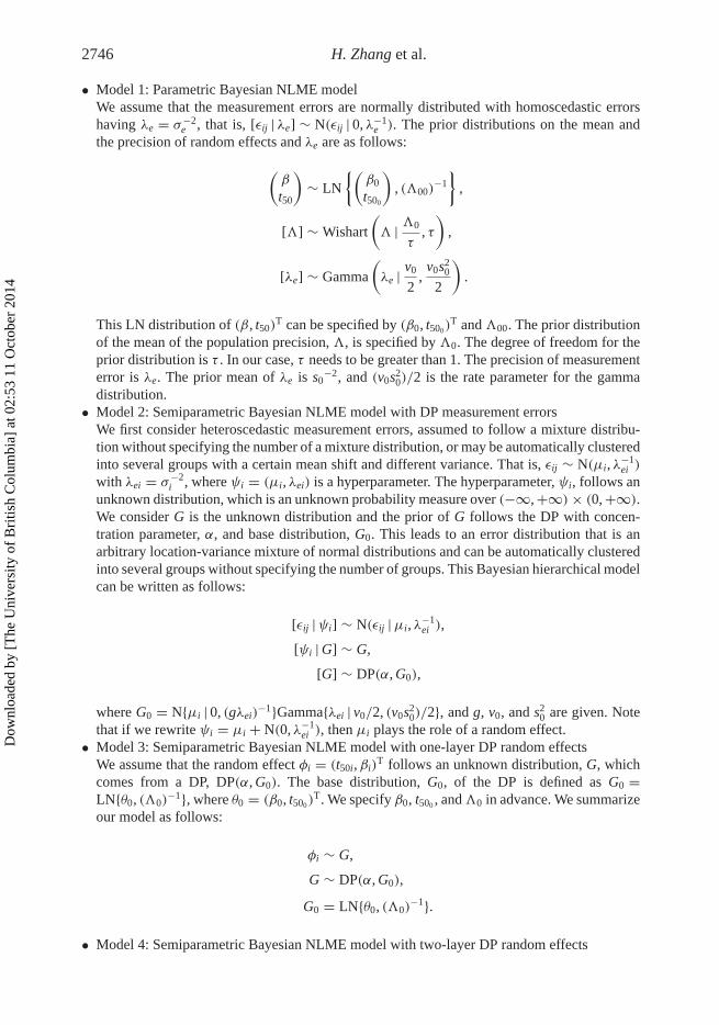
• Model 1: Parametric Bayesian NLME modelWe assume that the measurement errors are normally distributed with homoscedastic errorshaving λe = σ−2
e , that is, [εij | λe] ∼ N(εij | 0, λ−1e ). The prior distributions on the mean and
the precision of random effects and λe are as follows:
(β
t50
)∼ LN
{(β0
t500
), (�00)
−1
},
[�] ∼ Wishart
(� | �0
τ, τ
),
[λe] ∼ Gamma
(λe | v0
2,v0s2
0
2
).
This LN distribution of (β, t50)T can be specified by (β0, t500)
T and �00. The prior distributionof the mean of the population precision, �, is specified by �0. The degree of freedom for theprior distribution is τ . In our case, τ needs to be greater than 1. The precision of measurementerror is λe. The prior mean of λe is s0
−2, and (v0s20)/2 is the rate parameter for the gamma
distribution.• Model 2: Semiparametric Bayesian NLME model with DP measurement errors
We first consider heteroscedastic measurement errors, assumed to follow a mixture distribu-tion without specifying the number of a mixture distribution, or may be automatically clusteredinto several groups with a certain mean shift and different variance. That is, εij ∼ N(μi, λ
−1ei )
with λei = σ−2i , where ψi = (μi, λei) is a hyperparameter. The hyperparameter, ψi, follows an
unknown distribution, which is an unknown probability measure over (−∞, +∞)× (0, +∞).We consider G is the unknown distribution and the prior of G follows the DP with concen-tration parameter, α, and base distribution, G0. This leads to an error distribution that is anarbitrary location-variance mixture of normal distributions and can be automatically clusteredinto several groups without specifying the number of groups. This Bayesian hierarchical modelcan be written as follows:
[εij |ψi] ∼ N(εij |μi, λ−1ei ),
[ψi | G] ∼ G,
[G] ∼ DP(α, G0),
where G0 = N{μi | 0, (gλei)−1}Gamma{λei | v0/2, (v0s2
0)/2}, and g, v0, and s20 are given. Note
that if we rewrite ψi = μi + N(0, λ−1ei ), then μi plays the role of a random effect.
• Model 3: Semiparametric Bayesian NLME model with one-layer DP random effectsWe assume that the random effect φi = (t50i,βi)
T follows an unknown distribution, G, whichcomes from a DP, DP(α, G0). The base distribution, G0, of the DP is defined as G0 =LN{θ0, (�0)
−1}, where θ0 = (β0, t500)T. We specify β0, t500 , and�0 in advance. We summarize
our model as follows:
φi ∼ G,
G ∼ DP(α, G0),
G0 = LN{θ0, (�0)−1}.
• Model 4: Semiparametric Bayesian NLME model with two-layer DP random effects
Dow
nloa
ded
by [
The
Uni
vers
ity o
f B
ritis
h C
olum
bia]
at 0
2:53
11
Oct
ober
201
4
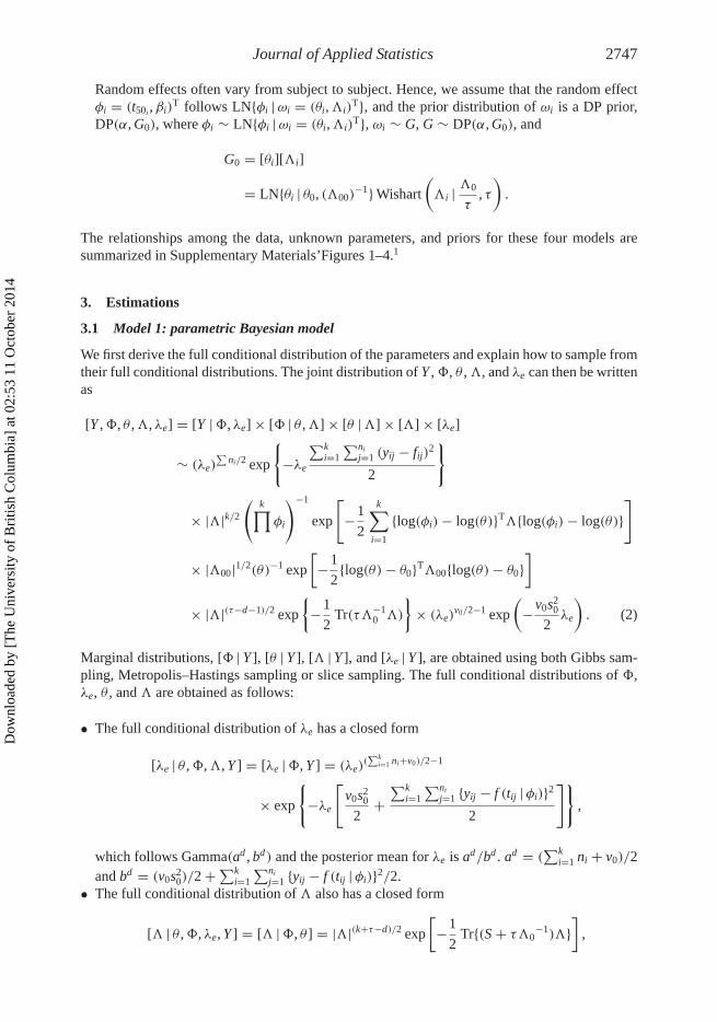
Journal of Applied Statistics 2747
Random effects often vary from subject to subject. Hence, we assume that the random effectφi = (t50i ,βi)
T follows LN{φi |ωi = (θi,�i)T}, and the prior distribution of ωi is a DP prior,
DP(α, G0), where φi ∼ LN{φi |ωi = (θi,�i)T}, ωi ∼ G, G ∼ DP(α, G0), and
G0 = [θi][�i]
= LN{θi | θ0, (�00)−1} Wishart
(�i | �0
τ, τ
).
The relationships among the data, unknown parameters, and priors for these four models aresummarized in Supplementary Materials’Figures 1–4.1
3. Estimations
3.1 Model 1: parametric Bayesian model
We first derive the full conditional distribution of the parameters and explain how to sample fromtheir full conditional distributions. The joint distribution of Y ,, θ ,�, and λe can then be writtenas
[Y ,, θ ,�, λe] = [Y |, λe] × [ | θ ,�] × [θ |�] × [�] × [λe]
∼ (λe)∑
ni/2 exp
{−λe
∑ki=1
∑nij=1 (yij − fij)2
2
}
× |�|k/2(
k∏φi
)−1
exp
[−1
2
k∑i=1
{log(φi)− log(θ)}T�{log(φi)− log(θ)}]
× |�00|1/2(θ)−1 exp
[−1
2{log(θ)− θ0}T�00{log(θ)− θ0}
]
× |�|(τ−d−1)/2 exp
{−1
2Tr(τ�−1
0 �)
}× (λe)
v0/2−1 exp
(−v0s2
0
2λe
). (2)
Marginal distributions, [ | Y ], [θ | Y ], [� | Y ], and [λe | Y ], are obtained using both Gibbs sam-pling, Metropolis–Hastings sampling or slice sampling. The full conditional distributions of ,λe, θ , and � are obtained as follows:
• The full conditional distribution of λe has a closed form
[λe | θ ,,�, Y ] = [λe |, Y ] = (λe)(∑k
i=1 ni+v0)/2−1
× exp
{−λe
[v0s2
0
2+∑k
i=1
∑nij=1 {yij − f (tij |φi)}2
2
]},
which follows Gamma(ad , bd) and the posterior mean for λe is ad/bd . ad = (∑k
i=1 ni + v0)/2and bd = (v0s2
0)/2 +∑ki=1
∑nij=1 {yij − f (tij |φi)}2/2.
• The full conditional distribution of � also has a closed form
[� | θ ,, λe, Y ] = [� |, θ ] = |�|(k+τ−d)/2 exp
[−1
2Tr{(S + τ�0
−1)�}]
,
Dow
nloa
ded
by [
The
Uni
vers
ity o
f B
ritis
h C
olum
bia]
at 0
2:53
11
Oct
ober
201
4
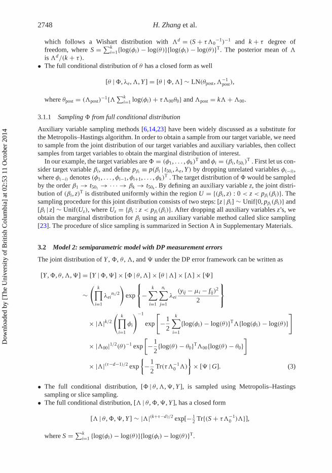
2748 H. Zhang et al.
which follows a Wishart distribution with �d = (S + τ�0−1)−1 and k + τ degree of
freedom, where S = ∑ki=1{log(φi)− log(θ)}{log(φi)− log(θ)}T. The posterior mean of �
is �d/(k + τ).• The full conditional distribution of θ has a closed form as well
[θ |, λe,�, Y ] = [θ |,�] ∼ LN(θpost,�−1post),
where θpost = (�post)−1{�∑k
i=1 log(φi)+ τ�00θ0} and �post = k�+�00.
3.1.1 Sampling from full conditional distribution
Auxiliary variable sampling methods [6,14,23] have been widely discussed as a substitute forthe Metropolis–Hastings algorithm. In order to obtain a sample from our target variable, we needto sample from the joint distribution of our target variables and auxiliary variables, then collectsamples from target variables to obtain the marginal distribution of interest.
In our example, the target variables are = (φ1, . . . ,φk)T and φi = (βi, t50i)
T . First let us con-sider target variable βi, and define pβi ≡ p(βi | t50i , λe, Y ) by dropping unrelated variables φ(−i),where φ(−i) denotes (φ1, . . . ,φi−1,φi+1, . . . ,φk)
T . The target distribution ofwould be sampledby the order β1 → t501 → · · · → βk → t50k . By defining an auxiliary variable z, the joint distri-bution of (βi, z)T is distributed uniformly within the region U = {(βi, z) : 0 < z < pβi(βi)}. Thesampling procedure for this joint distribution consists of two steps: [z |βi] ∼ Unif{0, pβi(βi)} and[βi | z] ∼ Unif(Uz), where Uz = {βi : z < pβi(βi)}. After dropping all auxiliary variables z’s, weobtain the marginal distribution for βi using an auxiliary variable method called slice sampling[23]. The procedure of slice sampling is summarized in Section A in Supplementary Materials.
3.2 Model 2: semiparametric model with DP measurement errors
The joint distribution of Y , , θ , �, and � under the DP error framework can be written as
[Y ,, θ ,�,�] = [Y |,�] × [ | θ ,�] × [θ |�] × [�] × [�]
∼(
k∏i=1
λeini/2
)exp
⎧⎨⎩−
k∑i=1
ni∑j=1
λei(yij − μi − fij)2
2
⎫⎬⎭
× |�|k/2(
k∏i=1
φi
)−1
exp
[−1
2
k∑i=1
{log(φi)− log(θ)}T�{log(φi)− log(θ)}]
× |�00|1/2(θ)−1 exp
[−1
2{log(θ)− θ0}T�00{log(θ)− θ0}
]
× |�|(τ−d−1)/2 exp
{−1
2Tr(τ�−1
0 �)
}× [� | G]. (3)
• The full conditional distribution, [ | θ ,�,�, Y ], is sampled using Metropolis–Hastingssampling or slice sampling.
• The full conditional distribution, [� | θ ,,�, Y ], has a closed form
[� | θ ,,�, Y ] ∼ |�|(k+τ−d)/2 exp[− 12 Tr{(S + τ�−1
0 )�}],
where S = ∑ki=1 {log(φi)− log(θ)}{log(φi)− log(θ)}T.
Dow
nloa
ded
by [
The
Uni
vers
ity o
f B
ritis
h C
olum
bia]
at 0
2:53
11
Oct
ober
201
4
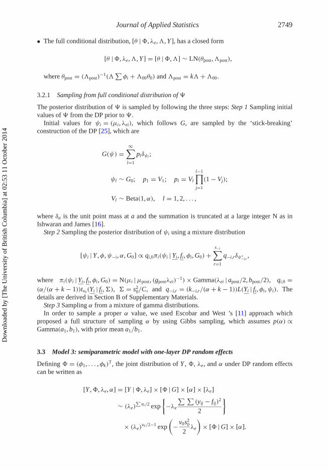
Journal of Applied Statistics 2749
• The full conditional distribution, [θ |, λe,�, Y ], has a closed form
[θ |, λe,�, Y ] = [θ |,�] ∼ LN(θpost,�post),
where θpost = (�post)−1(�
∑φi +�00θ0) and �post = k�+�00.
3.2.1 Sampling from full conditional distribution of �
The posterior distribution of � is sampled by following the three steps: Step 1 Sampling initialvalues of � from the DP prior to �.
Initial values for ψi = (μi, λei), which follows G, are sampled by the ‘stick-breaking’construction of the DP [25], which are
G(ψ) =∞∑
l=1
plδψl ;
ψl ∼ G0; p1 = V1; pl = Vl
l−1∏j=1
(1 − Vj);
Vl ∼ Beta(1,α), l = 1, 2, . . . ,
where δa is the unit point mass at a and the summation is truncated at a large integer N as inIshwaran and James [16].
Step 2 Sampling the posterior distribution of ψi using a mixture distribution
[ψi | Y ,φ,ψ−i,α, G0] ∝ qi,0πi(ψi | Yi, fi,φi, G0)+s−i∑r=1
q−i,rδψ∗−i,r
,
where πi(ψi | Yi, fi,φi, G0) = N(μi |μpost, (gpostλei)−1)× Gamma(λei | apost/2, bpost/2), qi,0 =
(α/(α + k − 1))tv0(Yi | fi,�), � = s20/C, and q−i,r = (k−i,r/(α + k − 1))L(Yi | fi,φi,ψi). The
details are derived in Section B of Supplementary Materials.Step 3 Sampling α from a mixture of gamma distributions.In order to sample a proper α value, we used Escobar and West ’s [11] approach which
proposed a full structure of sampling α by using Gibbs sampling, which assumes p(α) ∝Gamma(a1, b1), with prior mean a1/b1.
3.3 Model 3: semiparametric model with one-layer DP random effects
Defining = (φ1, . . . ,φk)T, the joint distribution of Y , , λe, and α under DP random effects
can be written as
[Y ,, λe,α] = [Y |, λe] × [ | G] × [α] × [λe]
∼ (λe)∑
ni/2 exp
{−λe
∑ ∑(yij − fij)2
2
}
× (λe)v0/2−1 exp
(−v0s2
0
2λe
)× [ | G] × [α].
Dow
nloa
ded
by [
The
Uni
vers
ity o
f B
ritis
h C
olum
bia]
at 0
2:53
11
Oct
ober
201
4
2750 H. Zhang et al.
• The full conditional distribution of λe is
[λe |, Y ] = (λe)(∑k
i=1 ni+v0)/2−1 exp
(−λe
[v0s2
0 +∑ki=1
∑nij=1 {yij − f (tij |φi)}2
2
]),
which is a gamma distribution,Gamma(ad , bd), with ad = ∑ki=1 ni + v0/2 and bd = {v0s2
0 +∑ki=1
∑nij=1 (yij − fij)2}/2.
• The posterior distribution of and α is sampled by the following three steps:Step 1 Sampling initial values of from the DP prior [ | G].Initial values for φi = (βi, t50i)
T, which is following G, are sampled by the ‘stick-breaking’construction of the DP [25].
Step 2 Sampling the posterior of φi using a mixture distribution [φi | Y ,φ−i,α, G0] (seeSection C of Supplementary Materials).
Step 3 Sampling α from a mixture of gamma distributions.In order to sample a proper α value, we perform the similar procedure which we explained
in Step 3 of Section 3.2.1.
3.4 Model 4: semiparametric model with two-layer DP random effects
The joint distributions of Y , , θ , �, and λe can be written as
[Y ,, θ ,�, λe] = [Y |, λe] × [ | θ ,�] × [θ |�] × [�] × [λe]
∼ (λe)∑
ni/2 exp
{−λe
∑ki=1
∑nij=1 (yij − fij)2
2
}
× |�i|k/2(
k∏φi
)−1
exp
[−1
2
k∑i=1
{log(φi)− log(θi)}T�i{log(φi)− log(θi)}]
× (λe)v0/2−1 exp
(−v0s2
0
2λe
)× [ωi = (θi,�i) | G], (4)
where G ∼ DP(α, G0) and G0 = [θi][�i] = LN{θi | θ0, (�00)−1} Wishart(�i |�0/τ , τ). Under
this framework, the sampling procedure is as follows:
• [φi | λe, θi,�i, Y ] can be sampled by Metropolis–Hastings sampling or slice sampling.• The full conditional distribution, [λe | θ ,,�, Y ], is
[λe | θ ,,�, Y ] ∼ (λe)∑
ni/2+a1−1 exp
(−λe
[b1 +
∑ki=1
∑nij=1 {yij − f (tij |φi)}2
2
]),
which is Gamma(ae, be) with ae = (∑k
i=1 ni)/2 + a1 and be = b1 +∑ki=1
∑nij=1{yij −
f (tij |φi)}2/2.• ωi = (θi,�i) is sampled from a DP mixture (see Section D of Supplementary Materials)
ωi ∼ α
α + k − 1p(φi)p(ωi |φi)+
s−i∑r=1
k−i,r
α + k − 1p(φi |ωr)δω∗
−i,r.
• Sampling α from the mixture of gamma distributions which exactly follows the method inSection 3.2.1.
Dow
nloa
ded
by [
The
Uni
vers
ity o
f B
ritis
h C
olum
bia]
at 0
2:53
11
Oct
ober
201
4
Journal of Applied Statistics 2751
4. Model selection
We are interested in selecting a model from a set of candidate models M1, M2, and M4. Morespecifically, M1 indicates the parametric NLME model, M2 indicates the NLME model with DPmeasurement errors, and M4 indicates the NLME model with two-layer DP random effects. Wedo not include M3 for model comparison with other models because M3 does not have populationparameters although we estimate individual parameters in M3.
For model selection, we may calculate the Bayes factor. However, in general, the Bayes fac-tor can be very sensitive to variations in the prior information of target parameters [1]. If theprior accurately represents one’s subjective belief about the target distribution, then such sen-sitivity is not a problem. However, the semiparametric Bayesian structure itself (DP prior) canbring the variation in the priors, when compared a parametric prior model. Petrone and Raftery[24] argue that the Bayes factor measures the degree of the improvement from the prior. Thevariation of the priors may come from the discrete nature of the DP and the infinite parameterspaces. Hence, Bayes factors may not be an appropriate option to compare a parametric modeland a semiparametric model. The other difficulty in calculating Bayes factors comes from ournonlinear likelihood function form and the DP prior structure, which increase the complexity ofthe approximations of the marginal likelihood.
To overcome these difficulties and drawbacks of the Bayes factor, Aitkin [1] proposed a pos-terior Bayes factor, which is the ratio of the pseudo-marginal likelihood. The pseudo-marginallikelihood weighs the likelihood functions by the posterior probabilities of the target parame-ters, rather than their prior probabilities. The use of the posterior mean has several advantages,including the reduced sensitivity to variations in the prior and the avoidance of the Lindley para-dox [20] in testing point null hypotheses. In our study, we incorporate posterior Bayes factor byadding a penalty term into the likelihood function, and propose a PPB factor to stably estimatevariance components in our nonlinear mixed model. We consider the penalty term as p( | θ ,�)which is the distribution of random effect in NLME model. We first describe the Bayes factorand explain the difficulties of the computation. We then show how to compute the PPB factorsand further discuss the cross-predictive densities.
4.1 Bayes factor
We wish to compare two models, Mr and M ′r , using the Bayes factor
Brr′ = p(Y | Mr)
p(Y | Mr′), (5)
where r = 1, 2, 4, r′ = 1, 2, 4, and r �= r′. Recall that M1 stands for a NLME model with para-metric priors, M2 stands for a NLME model with DP measurement errors, and M4 stands for aNLME model with two-layer DP random effects. The marginal likelihood given M1 is p(Y | M1).For ease of notation, we use p(Yi) for p(Yi | M1).
Chib [3] and Chib and Jeliazkov [5] estimated the marginal likelihood function. The proposedestimator of the marginal density on a logarithm scale is
log{p̂(Yi)} = log{p(Yi |φ∗i , ξ ∗)}︸ ︷︷ ︸
Element 1
+ log{p(φ∗i , ξ ∗)}︸ ︷︷ ︸
Element 2
− log{p(φ∗i , ξ ∗ | Yi)︸ ︷︷ ︸
Element 3
}, (6)
and this equation always holds for any φ∗i and ξ ∗. An arbitrary point in the parameter space is
marked by ‘∗’. This approach requires us to evaluate the likelihood function, the prior, and anestimate of the posterior.
The difficulty of the computation of Equation (6) comes from Element 3. The φi does nothave a closed from. In terms of the parametric prior setting, Chib [3] and Chib and Jeliazkov
Dow
nloa
ded
by [
The
Uni
vers
ity o
f B
ritis
h C
olum
bia]
at 0
2:53
11
Oct
ober
201
4
2752 H. Zhang et al.
[5] proposed a method to estimate the posterior probability of φi based on the unnormalizedposterior function. However, our models 2 and 4 assume that either λe or ωi = (θi,�i) is froma DP prior. This prior structure increases the computation complexity of Element 3, associatingthe unnormalized posterior function form.
4.2 PPB factor
In our study, we propose a PPB factor by adding a penalty term into the likelihood functionbecause our model has hierarchical structure, while a posterior Bayes factor cannot be used insuch complicated structure. We consider the penalty term as p( | θ ,�) which is the distributionof random effect in the NLME model.
The PPB factor with penalty term can expressed as
PPBrr′ = ps(Y | Mr)
ps(Y | Mr′), (7)
where the pseudo-marginal likelihood given model Mr is
ps(Y | Mr) =∫
Mr
p(Y |, λe)︸ ︷︷ ︸Likelihood
p( | θ ,�)︸ ︷︷ ︸Penalty
p(, θ ,�, λe | Y )︸ ︷︷ ︸Posterior
d dλe dθ rd�. (8)
It can be estimated by evaluating∑m
s=1 p(Y |s, λse)p(
s | θ s,�s)/m, where (s, λse, θ
s,�s) aregenerated from the posterior distribution p(, θ ,�, λe | Y ).
For the prediction problem, it is natural to assess the predictive ability of the model by usingcross-validation. The cross-validation predictive densities are proposed as
CVPD =∫
∫ξ
k∏i=1
ni∏j=1
p(yij |, ξ)p{, ξ | Y(−ij)} d dξ , (9)
where i = 1, . . . , k, j = 1, . . . , ni, and n = ∑k1 ni. In Equation (9), yij stands for a single
observation from a subject, and Y(−ij) stands for all observations except yij.
5. Simulation
In this section, simulation studies are conducted to evaluate the performances of models M1,M2, and M4. Nine scenarios, defined by the sample size and true model (TM) setting, are con-sidered to examine the properties of the model estimations and PPB factors. We consider thesimulation settings aresimilar to our gastric emptying study. In this simulation study, n individ-uals are simulated with m observation points per individual, expressed as tij, at [1450] min with50-min increments. The individuals, φi = (βi, t50i)
T, are generated from multivariate LNdistribu-tions with the mean (β, t50)
T and precision matrix �. This profile is generated for the individuali by adding independent normal errors with precision λe.
Three TM settings are considered:
• In TM setting 1, the measurement errors are from a non-mixture distribution and the ran-dom effect parameters are from a non-mixture population distribution as well. The populationmeans are β = 1.5 and t50 = 1.1, and the population precision is � = (
84 −1−1 88
). The parame-
ters (βi, t50i)T for individuals are generated from the LN distribution with the population means
and precision. Within subjects, the observations share the same individual parameters βi, t50i ,and the same error precision, λe = 15.
Dow
nloa
ded
by [
The
Uni
vers
ity o
f B
ritis
h C
olum
bia]
at 0
2:53
11
Oct
ober
201
4
Journal of Applied Statistics 2753
• In TM setting 2, we would assume the measurement errors are from a mixture of two distribu-tions and the random effect is still from a non-mixture population distribution. The populationmean and the population precision are the same as TM setting 1. Within subjects, the observa-tions share the same individual parameters βi, t50i , and the mixture of error precisions, λe = 5and λe = 20 with the probability, 0.5, for each.
• In TM setting 3, we assume the measurement errors are from a non-mixture distribution andthe random effect is from a mixture of two distributions. The population means are a mixtureof (β = 1.8, t50 = 1.6)T and (β = 0.6, t50 = 0.6)T with equal probability, 0.5, and the popula-tion precision is the same as TM setting 1. Within subjects, the observations share the sameindividual parameters βi, t50i , and the same error precision, λe = 15.
We assign three different sample sizes for each of the three TMs: (10 subjects and 10observations for each subject), (10 subjects and 20 observations for each subject), and (20subjects and 20 observations for each subject). Hence, the nine combinations of scenarios aresummarized:
• Scenario 1: TM setting 1 and (10 subjects and 10 observations for each subject).• Scenario 2: TM setting 2 and (10 subjects and 10 observations for each subject).• Scenario 3: TM setting 3 and (10 subjects and 10 observations for each subject).• Scenario 4: TM setting 1 and (10 subjects and 20 observations for each subject).• Scenario 5: TM setting 2 and (10 subjects and 20 observations for each subject).• Scenario 6: TM setting 3 and (10 subjects and 20 observations for each subject).• Scenario 7: TM setting 1 and (20 subjects and 20 observations for each subject).• Scenario 8: TM setting 2 and (20 subjects and 20 observations for each subject).• Scenario 9: TM setting 3 and (20 subjects and 20 observations for each subject).
For each scenario we would simulate 100 data sets. We use these simulated data sets to comparethree Bayesian hierarchical models, M1, M2, and M4 . The model evaluation results based on PPBfactors (7) are summarized in Table 1.
The penalized posterior marginal likelihood (8) of each candidate model is calculated for asimulated data set. We generate 100 data sets from each scenario and three models are imple-mented for each of these data sets. The logarithmic value of the penalized posterior marginallikelihood of each model for a given data set is calculated. As Kass and Raftery [17] men-tioned, there is strong evidence that the first model performs better than the second model whenthe Bayes factor is larger than 10 and decisive evidence when the Bayes factor is larger than100. In this paper, we take the value of logarithmic of the penalized posterior marginal likeli-hood, 4, as the cutoff of the significance. For each scenario, we count how many times a certainmodel is significantly better than other two. The comparison results are summarized in Table 1.We find that the three models have similar performances when the data setis generated from anon-mixture setting (scenarios 1, 4, and 7). The three models have similar performances underscenarios 1, 4, and 7. Taking into account the complexities of the three models, model 1 is theproper model because there are fewer computations. When the data sets are simulated from amixture of measurement errors and non-mixture of random effects (the scenarios 2, 5, and 8).We find that model 2 is always the best model, given the counts are 99, 100, and 100 (Table 1).Model 2, the semiparametric model with DP measurement error, can fit the data with a mixtureof measurement error best. In scenarios 3, 6, and 9 where there are non-mixture measurementerrors and a mixture of random effects, the counts, where the model 4 is the best model, are 89,91, and 100. We observe that model 4, the semiparametric model with two-layer DP random
Dow
nloa
ded
by [
The
Uni
vers
ity o
f B
ritis
h C
olum
bia]
at 0
2:53
11
Oct
ober
201
4
2754 H. Zhang et al.
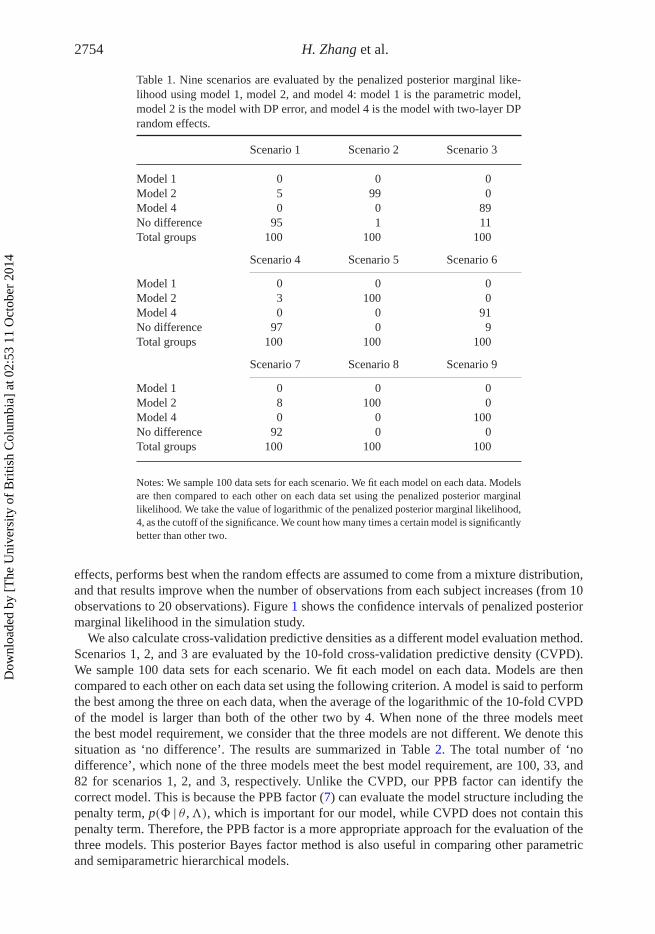
Table 1. Nine scenarios are evaluated by the penalized posterior marginal like-lihood using model 1, model 2, and model 4: model 1 is the parametric model,model 2 is the model with DP error, and model 4 is the model with two-layer DPrandom effects.
Scenario 1 Scenario 2 Scenario 3
Model 1 0 0 0Model 2 5 99 0Model 4 0 0 89No difference 95 1 11Total groups 100 100 100
Scenario 4 Scenario 5 Scenario 6
Model 1 0 0 0Model 2 3 100 0Model 4 0 0 91No difference 97 0 9Total groups 100 100 100
Scenario 7 Scenario 8 Scenario 9
Model 1 0 0 0Model 2 8 100 0Model 4 0 0 100No difference 92 0 0Total groups 100 100 100
Notes: We sample 100 data sets for each scenario. We fit each model on each data. Modelsare then compared to each other on each data set using the penalized posterior marginallikelihood. We take the value of logarithmic of the penalized posterior marginal likelihood,4, as the cutoff of the significance. We count how many times a certain model is significantlybetter than other two.
effects, performs best when the random effects are assumed to come from a mixture distribution,and that results improve when the number of observations from each subject increases (from 10observations to 20 observations). Figure 1 shows the confidence intervals of penalized posteriormarginal likelihood in the simulation study.
We also calculate cross-validation predictive densities as a different model evaluation method.Scenarios 1, 2, and 3 are evaluated by the 10-fold cross-validation predictive density (CVPD).We sample 100 data sets for each scenario. We fit each model on each data. Models are thencompared to each other on each data set using the following criterion. A model is said to performthe best among the three on each data, when the average of the logarithmic of the 10-fold CVPDof the model is larger than both of the other two by 4. When none of the three models meetthe best model requirement, we consider that the three models are not different. We denote thissituation as ‘no difference’. The results are summarized in Table 2. The total number of ‘nodifference’, which none of the three models meet the best model requirement, are 100, 33, and82 for scenarios 1, 2, and 3, respectively. Unlike the CVPD, our PPB factor can identify thecorrect model. This is because the PPB factor (7) can evaluate the model structure including thepenalty term, p( | θ ,�), which is important for our model, while CVPD does not contain thispenalty term. Therefore, the PPB factor is a more appropriate approach for the evaluation of thethree models. This posterior Bayes factor method is also useful in comparing other parametricand semiparametric hierarchical models.
Dow
nloa
ded
by [
The
Uni
vers
ity o
f B
ritis
h C
olum
bia]
at 0
2:53
11
Oct
ober
201
4

Journal of Applied Statistics 2755
(a) (b) (c)
(d) (e) (f)
(g) (h) (i)
Figure 1. The confidence intervals of penalized posterior marginal likelihood: 100 data sets are generatedfrom each of 9 scenarios. The penalized posterior marginal likelihood of three models are calculated for eachdata set. The boxplots are to compare the confidence intervals of penalized posterior marginal likelihoodsof three models under each scenario.
Table 2. Three scenarios are evaluated by the 10-fold CVPD: model 1 is theparametric model, model 2 is the model with DP error, and model 4 is the modelwith DP random effects.
Scenario 1 Scenario 2 Scenario 3
Model 1 0 0 14Model 2 0 67 1Model 4 0 0 3No difference 100 33 82Total groups 100 100 100
6. Application to equine gastric emptying data
The example for our study, which was described in Section 1, is from equine medicine. We fittedall four models. We provide results only from model 1, model 2, and model 4 because model 3
Dow
nloa
ded
by [
The
Uni
vers
ity o
f B
ritis
h C
olum
bia]
at 0
2:53
11
Oct
ober
201
4
2756 H. Zhang et al.
does not have population parameters. However, if it is requested, we can provide the results ofindividual parameter estimator.
6.1 Estimation results for the parametric NLME model (model 1)
We start with parametric Bayesian NLME model. In this case, [�] = Wishart(� |�0, τ) is theprior for the precision of the population mean. Given τ ≥ d + 1 and d = 2 we set τ to be 4.This choice of a small τ can lead to a large variance �0 which is a 2 × 2 identity matrix.[(β, t50)
T |�] ∼ LN{(β0, t500)T, (τ�)−1} is the prior for the population mean, where t500 = −0.7
and β0 = 0. The prior for the measurement error is [λe] = Gamma(λe | a1, b1) , where a1 = 1and b1 = 1.
We fit the NLME model with parametric priors, and the results are summarized in Supple-mentary Materials’ Tables 1 and 2. These results are based on 1000 runs after burn-in time.The medians of βi and t50i are given in the left half of Supplementary Materials’ Tables 1and 2, respectively. And ‘BCI25’ and ‘BCI975’ are 95% Bayesian lower and upper credibleintervals. From Supplementary Materials’ Table 2, we found the smallest value for t50i is 0.35(= t509 ), which is from horse 1916; the largest one is 3.36 (= t5016 ) for horse 1937. The popula-tion parameters are provided in Table 3. The median for t50, β, and �e are 1.12, 1.48, and 0.35,respectively.
6.2 Estimation results for the NLME model with DP errors (model 2)
In this case, G0 = N(μi | 0, (gλei)−1)Gamma(λei | a2/2, b2/2), where a2 = 1, b2 = 1, and g =
0.1. The prior for α is a Gamma(a3, b3), where a3 = 1 and b3 = 1. For other parameters we tookthe same setting as the parametric Bayesian model.
We fit the NLME model with DP errors, and the results are summarized in Tables 1 and 2.From Table 2, we notice the smallest value for t50i is 0.35 (= t509 ) which is from horse 1916,while the largest one is 3.35 (= t5016 ) which is from horse 1937. The population parameters arealso presented in Table 4. The median for t50 and β are 1.49 and 3.05, respectively. The mediansfor λi
e, i = 1, . . . , 21, vary.
6.3 Estimation results for the NLME model with two-layer DP random effects (model 4)
The medians of βi and t50i are given in the right part of Tables 1 and 2. From Table 2, we find thesmallest value for t50i is 0.37 (= t509 ), which is from horse 1916; the largest one is 3.36 (= t5016 )for horse 1937. The population parameters are summarized in Tables 5–7, and the median for λe
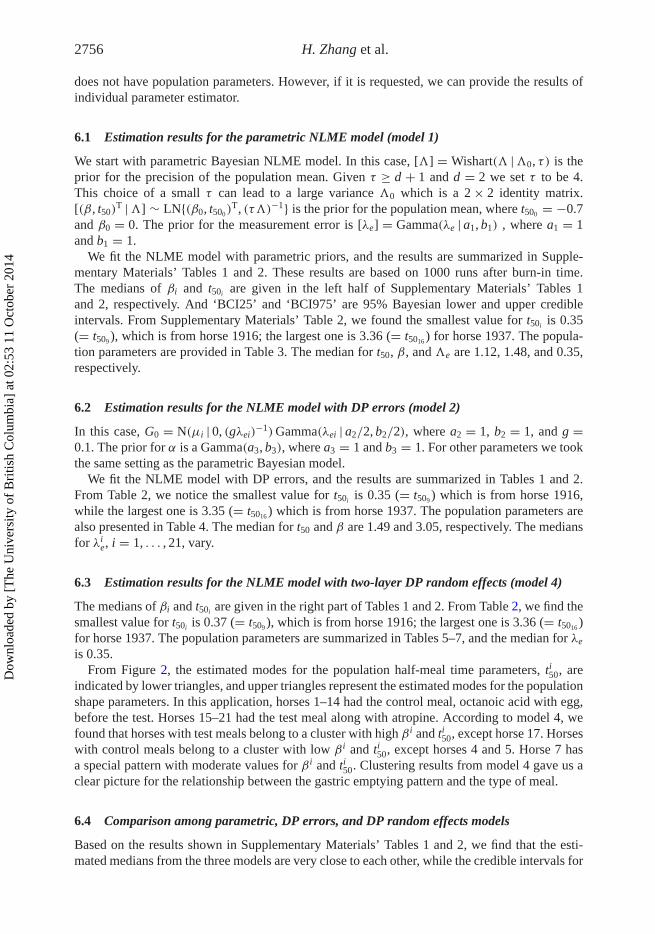
is 0.35.From Figure 2, the estimated modes for the population half-meal time parameters, ti50, are
indicated by lower triangles, and upper triangles represent the estimated modes for the populationshape parameters. In this application, horses 1–14 had the control meal, octanoic acid with egg,before the test. Horses 15–21 had the test meal along with atropine. According to model 4, wefound that horses with test meals belong to a cluster with high β i and ti50, except horse 17. Horseswith control meals belong to a cluster with low β i and ti50, except horses 4 and 5. Horse 7 hasa special pattern with moderate values for β i and ti50. Clustering results from model 4 gave us aclear picture for the relationship between the gastric emptying pattern and the type of meal.
6.4 Comparison among parametric, DP errors, and DP random effects models
Based on the results shown in Supplementary Materials’ Tables 1 and 2, we find that the esti-mated medians from the three models are very close to each other, while the credible intervals for
Dow
nloa
ded
by [
The
Uni
vers
ity o
f B
ritis
h C
olum
bia]
at 0
2:53
11
Oct
ober
201
4
Journal of Applied Statistics 2757
Figure 2. Estimated modes for the half-meal time and shape parameters (model 4): lower triangles representthe estimated modes for the population half-meal time parameters, ti50, i = 1, . . . , 21. Upper triangles rep-resent the estimated modes for the shape parameters, β i, for the ith individual. Horses1–14 had the controlmeal before the test. Horses 15–21 had the test meal along with atropine before test.
the NLME model with DP errors and random effects are narrower than those of the parametricNLME model. We further compare the three models using the PPB factor. From SupplementaryMaterials’ Figures 6 and 7, we also observe that the individual fitted curves from the three mod-els are overlapped. Hence the estimated variance could be a crucial factor in identifying the rightmodel.
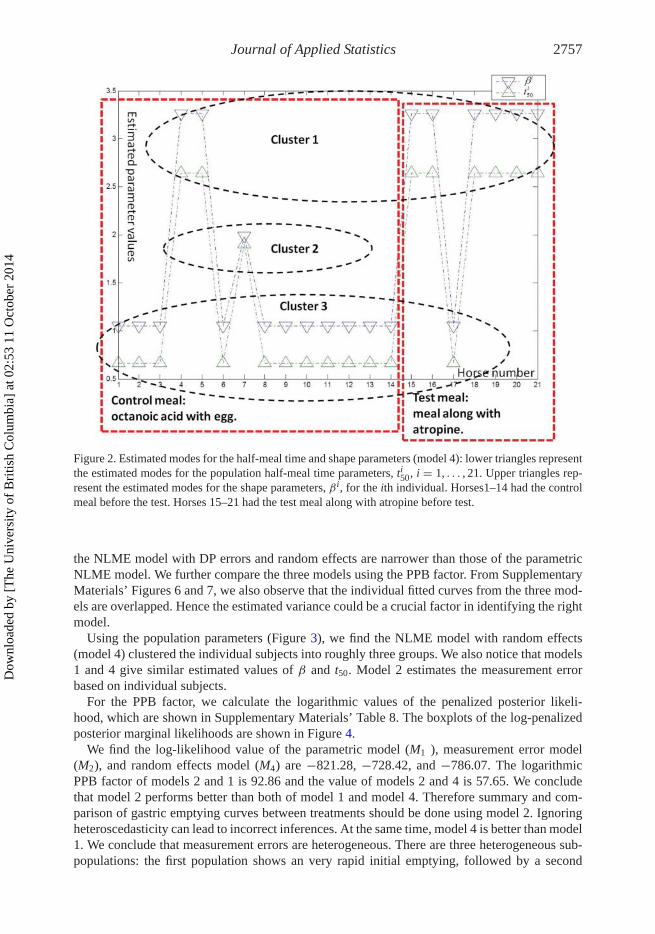
Using the population parameters (Figure 3), we find the NLME model with random effects(model 4) clustered the individual subjects into roughly three groups. We also notice that models1 and 4 give similar estimated values of β and t50. Model 2 estimates the measurement errorbased on individual subjects.
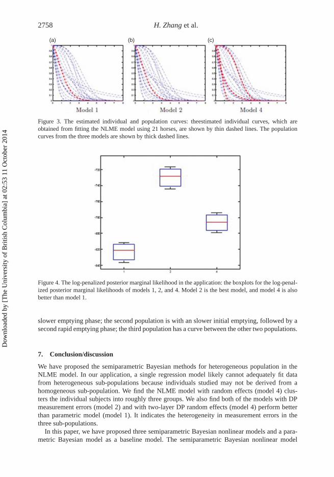
For the PPB factor, we calculate the logarithmic values of the penalized posterior likeli-hood, which are shown in Supplementary Materials’ Table 8. The boxplots of the log-penalizedposterior marginal likelihoods are shown in Figure 4.
We find the log-likelihood value of the parametric model (M1 ), measurement error model(M2), and random effects model (M4) are −821.28, −728.42, and −786.07. The logarithmicPPB factor of models 2 and 1 is 92.86 and the value of models 2 and 4 is 57.65. We concludethat model 2 performs better than both of model 1 and model 4. Therefore summary and com-parison of gastric emptying curves between treatments should be done using model 2. Ignoringheteroscedasticity can lead to incorrect inferences. At the same time, model 4 is better than model1. We conclude that measurement errors are heterogeneous. There are three heterogeneous sub-populations: the first population shows an very rapid initial emptying, followed by a second
Dow
nloa
ded
by [
The
Uni
vers
ity o
f B
ritis
h C
olum
bia]
at 0
2:53
11
Oct
ober
201
4
2758 H. Zhang et al.
(a) (b) (c)
Figure 3. The estimated individual and population curves: theestimated individual curves, which areobtained from fitting the NLME model using 21 horses, are shown by thin dashed lines. The populationcurves from the three models are shown by thick dashed lines.
Figure 4. The log-penalized posterior marginal likelihood in the application: the boxplots for the log-penal-ized posterior marginal likelihoods of models 1, 2, and 4. Model 2 is the best model, and model 4 is alsobetter than model 1.
slower emptying phase; the second population is with an slower initial emptying, followed by asecond rapid emptying phase; the third population has a curve between the other two populations.
7. Conclusion/discussion
We have proposed the semiparametric Bayesian methods for heterogeneous population in theNLME model. In our application, a single regression model likely cannot adequately fit datafrom heterogeneous sub-populations because individuals studied may not be derived from ahomogeneous sub-population. We find the NLME model with random effects (model 4) clus-ters the individual subjects into roughly three groups. We also find both of the models with DPmeasurement errors (model 2) and with two-layer DP random effects (model 4) perform betterthan parametric model (model 1). It indicates the heterogeneity in measurement errors in thethree sub-populations.
In this paper, we have proposed three semiparametric Bayesian nonlinear models and a para-metric Bayesian model as a baseline model. The semiparametric Bayesian nonlinear model
Dow
nloa
ded
by [
The
Uni
vers
ity o
f B
ritis
h C
olum
bia]
at 0
2:53
11
Oct
ober
201
4
Journal of Applied Statistics 2759
with two-layer DP random effects is useful because it automatically cluster heterogeneoussub-populations without specifying the number of different groups.
The semiparametric Bayesian nonlinear model with two-layer DP random effects has twoattractive properties. When we implement a nonlinear model with one-layer DP random effects,the marginal likelihood from the DP posterior is very difficult to compute in terms of the non-linear form of the likelihood function. However, the nonlinear model with two-layer DP randomeffects constructs the marginal likelihood which does not depend on the likelihood function. Themarginal likelihood in a DP posterior has a closed form as long as we assign the proper priorfor the individual subjects and the base distribution for the population DP prior. This propertycan dramatically reduce the computation complexity of the nonlinear random effects model. Thesecond attractive property of this model is that the model structure allows us to perform modelselection on the semiparametric random effects model, DP measurement error model, and theparametric random effects model. All of these models have a two-layer structure on the randomeffects. We point out that a semiparametric model with one-layer random effects is not compara-ble with the DP measurement error model and the parametric random effects model because theone-layer random effects models do not have population parameters.
In this study, we also propose a model selection method, the PPB factor. The constraint onrandom effects is added into the PPB factor as a penalty term. The PPB factor marginalizes thelikelihood function by the posterior distribution of the two-layer parameter. The prior densityfor computing Bayes factors is very flexible under the DP prior setting, where it makes theBayes factor’s result sensitive to the value of prior density. In order to compare the two-layerDP random effects model, the DP measurement error model, and the parametric random effectsmodel, we calculate the marginal penalized likelihood over the posterior distribution of the two-layer parameter. Based on the simulation study, the PPB factor is a robust and stable method touse to compare the parametric and semiparametric Bayesian hierarchical models.
Acknowledgements
This research was supported by grants from National Science Foundation (NSF-CNS0964680 and NSF-CNS1115839).
Note
1. Supplementary content may be viewed online at http://dx.doi.org/10.1080/02664763.2014.928848
References
[1] M. Aitkin, Posterior Bayes factors, J. R. Stat. Soc. Ser. B (Methodol.) 53 (1991), pp. 111–142.[2] D. Anderson, D. Appl, D. Bartholomeusz, I.D. Kirkwood, B.E. Chatterton, G. Summersides, S. Penglis, M. Appl, T.
Kuchel, and L. Sansom, Liquid gastric emptying in the pig: Effect of concentration of inhaled isoflurance, J. Nucl.Med. 43 (2002), pp. 968–971.
[3] S. Chib, Marginal likelihood from the Gibbs output, J. Am. Stat. Assoc. 90 (1995), pp. 1313–1321.[4] S. Chib and E. Greenberg, Additive cubic spline regression with Dirichlet process mixture errors, J. Econ. 156
(2010), pp. 322–336.[5] S. Chib and I. Jeliazkov, Marginal likelihood from the Metropolis–Hastings output, J. Am. Stat. Assoc. 96 (2001),
pp. 270–281.[6] P. Damien, J. Wakefield, and S. Walker, Gibbs sampling for Bayesian non-conjugate and hierarchical models by
using auxiliary variables, J. R. Stat. Soc. B 61 (1999), pp. 331–344.[7] M. Davidian and D.M. Giltinan, Nonlinear Models for Repeated Measurement Data, Chapman and Hall/CRC, Boca
Raton, FL, 1995.[8] A.P. Dempster, N.M. Laird, and D.B. Rubin, Maximum likelihood from incomplete data via the EM algorithm,
J. R. Stat. Soc. Ser. B 39 (1977), pp. 1–38.
Dow
nloa
ded
by [
The
Uni
vers
ity o
f B
ritis
h C
olum
bia]
at 0
2:53
11
Oct
ober
201
4
2760 H. Zhang et al.
[9] J.D. Elashoff, T.J. Reedy, and J.H. Meyer, Analysis of gastric emptying data, Gastroenterology 83 (1982), pp.1306–1312.
[10] J.D. Elashoff, T.J. Reedy, and J.H. Meyer, Methods for gastric emptying data (letter to the editor), Gastrointest.Liver Physiol. 7 (1983), pp. G701–G702.
[11] M.D. Escobar and M. West, Bayesian density estimation and inference using mixtures, J. Am. Stat. Assoc. 90(1995), pp. 577–588.
[12] T.S. Ferguson, A Bayesian analysis of some nonparametric problems, Ann. Stat. 1 (1973), pp. 209–230.[13] A. Gelman and X.-L. Meng, Simulating normalizing constants: From importance sampling to bridge sampling to
path sampling, Stat. Sci. 13 (1998), pp. 163–185.[14] D.M. Higdon, Auxiliary variable methods for Markov chain Monte Carlo with applications, J. Am. Stat. Assoc. 93
(1998), pp. 585–595.[15] B. Hyett, F.J. Martinez, B.M. Gill, S. Mehra, A. Lembo, C.P. Kelly, and D.A. Leffler, Delayed radionucleotide
gastric emptying studies predict morbidity in diabetics with symptoms of gastroparesis, J. Nucl. Med. 137 (2009),pp. 445–452.
[16] H. Ishwaran and L.F. James, Gibbs sampling methods for stick-breaking priors, J. Am. Stat. Assoc. 96 (2001), pp.161–173 (Theory and Methods).
[17] R.E. Kass and A.E. Raftery, Bayes factors, J. Am. Stat. Assoc. 90 (1995), pp. 773–595.[18] K.P. Kleinmanm and J.G. Ibrahim, A semiparametric Bayesian approach to the random effects model, Biometrics
54 (1998), pp. 921–938.[19] M. Kyung, J. Gill, and G. Casella, Estimation in Dirichlet random effects models, Ann. Stat. 38 (2010), pp. 979–
1009.[20] D.V. Lindley, A statistical paradox, Biometrika 44 (1957), pp. 187–192.[21] M.J. Lindstrom and D.M. Bates, Nonlinear mixed effects models for repeated measures data, Biometrics 46 (1990),
pp. 673–687.[22] R.M. Neal, Markov chain sampling methods for Dirichlet process mixture models, J. Comput. Graph. Stat. 9 (2000),
249–265.[23] R.M. Neal, Slice sampling, Ann. Stat. 31 (2003), pp. 705–767.[24] S. Petrone and A.E. Raftery, A note on the Dirichlet process prior in Bayesian nonparametric inference with partial
exchangeability, Stat. Probab. Lett. 36 (1997), pp. 69–83.[25] J. Sethuraman, A constructive definition of Dirichlet priors, Stat. Sin. 4 (1994), pp. 639–650.[26] B. Shahbaba and R.M. Neal, Nonlinear models using Dirichlet process mixtures, J. Mach. Learn. Res. 10 (2009),
pp. 1829–1850.[27] J.L. Steimer, A. Mallet, J.L. Golmard, and J.F. Boisvieux, Alternative approaches to estimation of population phar-
macokinetic parameters: Comparison with the nonlinear mixed-effect model, Drug Metab. Rev. 15 (1984), pp.265–292.
[28] D.G.M. Sutton, T. Preston, N.D. Cohen, S. Love, and A.J. Roussel, The effects of xylazine, detomidine,acepromazine, and butorphanol on equine solid-phase gastric emptying, Equine Vet. J. 34 (2002), pp. 486–492.
[29] J. Wang, Dirichlet processes in nonlinear mixed effects models, Commun. Stat. Simul. Comput. 39 (2010), pp.539–556.
Dow
nloa
ded
by [
The
Uni
vers
ity o
f B
ritis
h C
olum
bia]
at 0
2:53
11
Oct
ober
201
4