Expert Systems with Applications 40 (2013) 7069–7079

Contents lists available at SciVerse ScienceDirect

Expert Systems with Applications

journal homepage: www.elsevier .com/locate /eswa

Semi-supervised object recognition based on Connected ImageTransformations

0957-4174/$ - see front matter � 2013 Elsevier Ltd. All rights reserved.http://dx.doi.org/10.1016/j.eswa.2013.06.029

⇑ Corresponding author. Tel.: +34 942200919x802; fax: +34 942201488.E-mail addresses: steven@gtas.dicom.unican.es (S. Van Vaerenbergh),

ignacio@gtas.dicom.unican.es (I. Santamaría), paoloemilio.barbano@yale.edu(P.E. Barbano).

Steven Van Vaerenbergh a,⇑, Ignacio Santamaría a, Paolo Emilio Barbano b

a Dept. of Communications Engineering, University of Cantabria, Plaza de la Ciencia s/n, Santander, 39005, Spainb Dept. of Mathematics, Yale University, PO Box 208283, New Haven, CT 06520-8283, USA

a r t i c l e i n f o

Keywords:Semi-supervised classificationObject recognitionConnectivityDeformation modelsLow-density separation

a b s t r a c t

We present a novel semi-supervised classifier model based on paths between unlabeled and labeled datathrough a sequence of local pattern transformations. A reliable measure of path-length is proposed thatcombines a local dissimilarity measure between consecutive patters along a path with a global, connec-tivity-based metric. We apply this model to problems of object recognition, for which we propose a prac-tical classification algorithm based on sequences of ‘‘Connected Image Transformations’’ (CIT).Experimental results on four popular image benchmarks demonstrate how the proposed CIT classifieroutperforms state-of-the-art semi-supervised techniques. The results are particularly significant whenonly a very small number of labeled patterns is available: the proposed algorithm obtains a generaliza-tion error of 4.57% on the MNIST data set trained on 2000 randomly chosen patterns with only 10 labeledpatterns per digit class.

� 2013 Elsevier Ltd. All rights reserved.

1. Introduction

In many object recognition problems, obtaining labeled data is atime-consuming and expensive task, whereas large unlabeled datasets are usually available. This is particularly true in problemsinvolving high-dimensional data, such as handwritten digit recog-nition, text categorization (Joachims, 1998), protein classification(Weston, Leslie, Zhou, Elisseeff, & Noble, 2004) or hyper-spectraldata classification (Rajan, Ghosh, & Crawford, 2008). In such sce-narios it is desirable to develop semi-supervised learning tech-niques, as these allow to exploit the available unlabeled dataconcurrently with the labeled training data. We focus on recogni-tion problems in which many instances of each object are availablefor training, and each instance differs only slightly from another in-stance of the same object. This is typically the case in handwrittendigit and face recognition systems, but it occurs more generally in awide variety of image recognition problems where series of spa-tially or temporally related patterns are available. In this case,the available instances of an object usually relate to each otherby transformations such as rotations, scalings and small nonlinearaxis deformations.

A large number of semi-supervised learning techniques havebeen proposed in the last years, for instance (Belkin, Niyogi, & Sin-

dhwani, 2006; Cohen, Cozman, Sebe, Cirelo, & Huang, 2004;Fischer, Roth, & Buhmann, 2004; Jaakkola & Szummer, 2002;Szlam, Maggioni, & Coifman, 2008; Wang & Zhang, 2007; Zhu,2005; Zhu, Ghahramani, & Lafferty, 2003; Zhou, Bousquet, Lal,Weston, & Schölkopf, 2004). The success of these techniques reliesmainly on two key assumptions: (i) the data lie on a manifold ofmuch lower dimensionality than the data dimension itself (mani-fold assumption) (Belkin et al., 2006); and (ii) data points belong-ing to the same high-density region are likely to belong to the sameclass (cluster assumption) (Fischer et al., 2004). Both assumptionscan be interpreted in terms of data similarity and distances. In thissense, the manifold assumption states that local variations in thedata should only involve variations of a small number of parame-ters. This property is illustrated in Fig. 1, which shows a numberof handwritten instances of the number 3: although the datadimensionality is high, most local variations can be described byfew parameters, such as line thickness, skew and rotation. There-fore, the manifold assumption leads naturally to the concept of alocal distance between patterns. Several algorithms exploit themanifold assumption, e.g. (Belkin & Niyogi, 2002), by estimatingthe marginal distribution underlying the data and training a classi-fier on the manifold itself.

The cluster assumption states that two data points should be-long to the same class if they can be connected by a path that liesexclusively in a region of high density. This assumption, which wasexploited for instance in Fischer et al. (2004) and Chapelle and Zien(2005), allows to define a global distance measure betweenpatterns that lie further apart. Specifically, the global distance

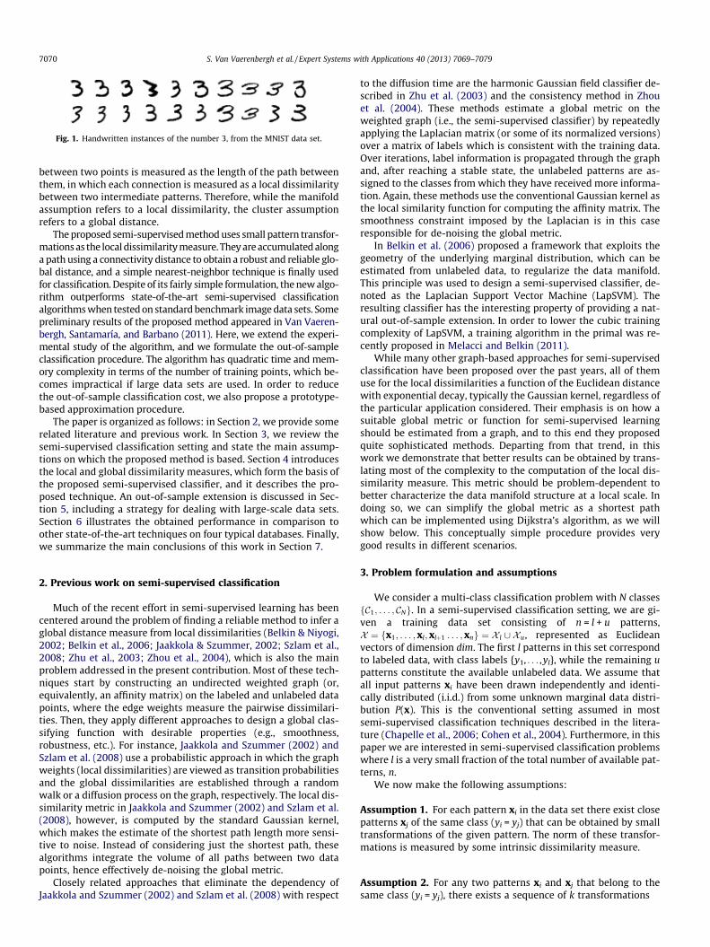
Fig. 1. Handwritten instances of the number 3, from the MNIST data set.

7070 S. Van Vaerenbergh et al. / Expert Systems with Applications 40 (2013) 7069–7079

between two points is measured as the length of the path betweenthem, in which each connection is measured as a local dissimilaritybetween two intermediate patterns. Therefore, while the manifoldassumption refers to a local dissimilarity, the cluster assumptionrefers to a global distance.

The proposed semi-supervised method uses small pattern transfor-mations as the local dissimilarity measure. They are accumulated alonga path using a connectivity distance to obtain a robust and reliable glo-bal distance, and a simple nearest-neighbor technique is finally usedfor classification. Despite of its fairly simple formulation, the new algo-rithm outperforms state-of-the-art semi-supervised classificationalgorithms when tested on standard benchmark image data sets. Somepreliminary results of the proposed method appeared in Van Vaeren-bergh, Santamaría, and Barbano (2011). Here, we extend the experi-mental study of the algorithm, and we formulate the out-of-sampleclassification procedure. The algorithm has quadratic time and mem-ory complexity in terms of the number of training points, which be-comes impractical if large data sets are used. In order to reducethe out-of-sample classification cost, we also propose a prototype-based approximation procedure.

The paper is organized as follows: in Section 2, we provide somerelated literature and previous work. In Section 3, we review thesemi-supervised classification setting and state the main assump-tions on which the proposed method is based. Section 4 introducesthe local and global dissimilarity measures, which form the basis ofthe proposed semi-supervised classifier, and it describes the pro-posed technique. An out-of-sample extension is discussed in Sec-tion 5, including a strategy for dealing with large-scale data sets.Section 6 illustrates the obtained performance in comparison toother state-of-the-art techniques on four typical databases. Finally,we summarize the main conclusions of this work in Section 7.

2. Previous work on semi-supervised classification

Much of the recent effort in semi-supervised learning has beencentered around the problem of finding a reliable method to infer aglobal distance measure from local dissimilarities (Belkin & Niyogi,2002; Belkin et al., 2006; Jaakkola & Szummer, 2002; Szlam et al.,2008; Zhu et al., 2003; Zhou et al., 2004), which is also the mainproblem addressed in the present contribution. Most of these tech-niques start by constructing an undirected weighted graph (or,equivalently, an affinity matrix) on the labeled and unlabeled datapoints, where the edge weights measure the pairwise dissimilari-ties. Then, they apply different approaches to design a global clas-sifying function with desirable properties (e.g., smoothness,robustness, etc.). For instance, Jaakkola and Szummer (2002) andSzlam et al. (2008) use a probabilistic approach in which the graphweights (local dissimilarities) are viewed as transition probabilitiesand the global dissimilarities are established through a randomwalk or a diffusion process on the graph, respectively. The local dis-similarity metric in Jaakkola and Szummer (2002) and Szlam et al.(2008), however, is computed by the standard Gaussian kernel,which makes the estimate of the shortest path length more sensi-tive to noise. Instead of considering just the shortest path, thesealgorithms integrate the volume of all paths between two datapoints, hence effectively de-noising the global metric.

Closely related approaches that eliminate the dependency ofJaakkola and Szummer (2002) and Szlam et al. (2008) with respect

to the diffusion time are the harmonic Gaussian field classifier de-scribed in Zhu et al. (2003) and the consistency method in Zhouet al. (2004). These methods estimate a global metric on theweighted graph (i.e., the semi-supervised classifier) by repeatedlyapplying the Laplacian matrix (or some of its normalized versions)over a matrix of labels which is consistent with the training data.Over iterations, label information is propagated through the graphand, after reaching a stable state, the unlabeled patterns are as-signed to the classes from which they have received more informa-tion. Again, these methods use the conventional Gaussian kernel asthe local similarity function for computing the affinity matrix. Thesmoothness constraint imposed by the Laplacian is in this caseresponsible for de-noising the global metric.

In Belkin et al. (2006) proposed a framework that exploits thegeometry of the underlying marginal distribution, which can beestimated from unlabeled data, to regularize the data manifold.This principle was used to design a semi-supervised classifier, de-noted as the Laplacian Support Vector Machine (LapSVM). Theresulting classifier has the interesting property of providing a nat-ural out-of-sample extension. In order to lower the cubic trainingcomplexity of LapSVM, a training algorithm in the primal was re-cently proposed in Melacci and Belkin (2011).

While many other graph-based approaches for semi-supervisedclassification have been proposed over the past years, all of themuse for the local dissimilarities a function of the Euclidean distancewith exponential decay, typically the Gaussian kernel, regardless ofthe particular application considered. Their emphasis is on how asuitable global metric or function for semi-supervised learningshould be estimated from a graph, and to this end they proposedquite sophisticated methods. Departing from that trend, in thiswork we demonstrate that better results can be obtained by trans-lating most of the complexity to the computation of the local dis-similarity measure. This metric should be problem-dependent tobetter characterize the data manifold structure at a local scale. Indoing so, we can simplify the global metric as a shortest pathwhich can be implemented using Dijkstra’s algorithm, as we willshow below. This conceptually simple procedure provides verygood results in different scenarios.

3. Problem formulation and assumptions

We consider a multi-class classification problem with N classesfC1; . . . ; CNg. In a semi-supervised classification setting, we are gi-ven a training data set consisting of n = l + u patterns,X ¼ fx1; . . . ;xl;xlþ1 . . . ;xng ¼ X l [ Xu, represented as Euclideanvectors of dimension dim. The first l patterns in this set correspondto labeled data, with class labels {y1, . . . ,yl}, while the remaining upatterns constitute the available unlabeled data. We assume thatall input patterns xi have been drawn independently and identi-cally distributed (i.i.d.) from some unknown marginal data distri-bution P(x). This is the conventional setting assumed in mostsemi-supervised classification techniques described in the litera-ture (Chapelle et al., 2006; Cohen et al., 2004). Furthermore, in thispaper we are interested in semi-supervised classification problemswhere l is a very small fraction of the total number of available pat-terns, n.

We now make the following assumptions:

Assumption 1. For each pattern xi in the data set there exist closepatterns xj of the same class (yi = yj) that can be obtained by smalltransformations of the given pattern. The norm of these transfor-mations is measured by some intrinsic dissimilarity measure.

Assumption 2. For any two patterns xi and xj that belong to thesame class (yi = yj), there exists a sequence of k transformations

S. Van Vaerenbergh et al. / Expert Systems with Applications 40 (2013) 7069–7079 7071

xj ¼ Tk � Tk�1 � � � � � T2 � T1ðxiÞ; ð1Þ

which is both short (i.e. the total number of transformations k issmall), and well connected (i.e. the norm of the transformation be-tween two consecutive patterns along the path is also small). Thesesequences are referred to as consistent. Accordingly, if two patternsxi and xj belong to different classes (yi – yj), all possible sequencesof transformations between xi and xj are either very long (i.e.k� 1), or are not well connected (i.e. the connecting path containsat least one weak link formed by two distant patterns).

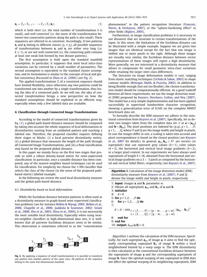
The first assumption is built upon the standard manifoldassumption. In particular, it supposes that most local intra-classvariations can be covered by a small number of parameters. Thesecond assumption is equivalent to the standard cluster assump-tion, and its formulation is similar to the concepts of local and glo-bal consistency discussed in Zhou et al. (2004) (see Fig. 2).

The applied transformations Ti of a consistent sequence shouldhave limited flexibility, since otherwise any two patterns could betransformed one into another by a single transformation, thus los-ing the idea of a connected path. As we will see, the idea of con-nected transformations brings a new perspective on how thestandard assumptions should be exploited in an efficient way,especially when only a few labeled data are available.

4. Classification through Connected Image Transformations

According to the model of connected transformations given byEq. (1), a global path-based distance measure should be computedby taking into account the whole sequence of local deformations ordissimilarities starting from an unlabeled pattern and reaching alabeled one. Therefore, the proposed classifier requires definingthree stages or blocks: (i) a local pairwise dissimilarity metric,(ii) a global distance that measures the length of the path throughall Connected Image Transformations, and (iii) a final classificationstep based on the proposed global distance.

In this paper we mainly focus on the first two stages that pro-vide us with a robust density-based metric for semi-supervisedclassification. In particular, once a suitable distance has been com-puted, any of the nearest-neighbor based techniques can be usedfor classification. For simplicity we choose the 1-NN classifier thatselects the class of the closest (in the sense of the proposed path-based metric) labeled example.

In the following we review the used local dissimilarity measureand the global path-based distance.

4.1. Dissimilarity based on local deformations

While the Euclidean distance between patterns is often used asa dissimilarity measure in graph-based semi-supervised classifica-tion problems (see for instance Belkin & Niyogi, 2002; Belkin et al.,2006; Chapelle et al., 2006; Jaakkola & Szummer, 2002; Szlamet al., 2008; Zhu et al., 2003; Zhou et al., 2004), it is not necessarilythe most suitable local dissimilarity. Especially when using near-est-neighbor classifiers in high-dimensional data sets, it is well-known that all pairwise Euclidean distances seem to be similar.This observation is sometimes referred to as the ‘‘concentration

Fig. 2. By applying a sequence of small transformations it is possible to transformany pattern into another pattern of the same class. All patterns of the sequencebelong to the same low-dimensional manifold.

phenomenon’’ in the pattern recognition literature (Francois,Wertz, & Verleysen, 2007), or the ‘‘sphere-hardening effect’’ inother fields (Biglieri, 2005).

Furthermore, in image classification problems it is necessary touse distances that are invariant to certain transformations of theinput. In this sense, the limitations of the Euclidean distance canbe illustrated with a simple example. Suppose we are given twoimages that are identical except for the fact that one image isshifted one or more pixels to the right. Although these imagesare visually very similar, the Euclidean distance between vectorrepresentations of these images will report a high dissimilarity.More generally, we are interested in a dissimilarity measure thatallows to compensate for small geometric intra-class variationswhile retaining the larger inter-class differences.

The literature on image deformation models is vast, rangingfrom elastic matching techniques (Uchida & Sakoe, 2003) to shapecontour models (Belongie, Malik, & Puzicha, 2002). In addition tobeing flexible enough (but not too flexible), the chosen transforma-tion model should be computationally efficient. As a good tradeoffbetween all these requirements, we use the image distortion mod-el (IDM) proposed by Keysers, Deselaers, Gollan, and Ney (2007).This model has a very simple implementation and has been appliedsuccessfully in supervised handwritten character recognition,showing a generalization error of 0.54% on the complete MNISTbenchmark data set.

To formally describe the IDM measure we adhere to the nota-tional convention from Keysers et al. (2007). Specifically, let us de-note two images taken from the complete data set X as a = {apq}and b = {bpq}. The pixel positions are indexed by (p,q), p = 1, . . . ,P;q = 1, . . . ,Q, where P and Q are the image width and height in pixels.In case the images differ in size, a scaling is taken into account andpixel correspondence is based on the closest position (see Keyserset al., 2007 for details). In general, apq;bpq 2 Rh are vectors (orsuperpixels) that can represent grey values (h = 1), color values(h = 3), the horizontal and vertical local image gradients (h = 2),or a larger pixel context. In our experiments we have always usedsuperpixels of length h = 18, obtained from the horizontal and ver-tical image gradients on a 3 � 3 patch as computed by the horizon-tal and vertical Sobel filters, respectively (see Keysers et al., 2007).

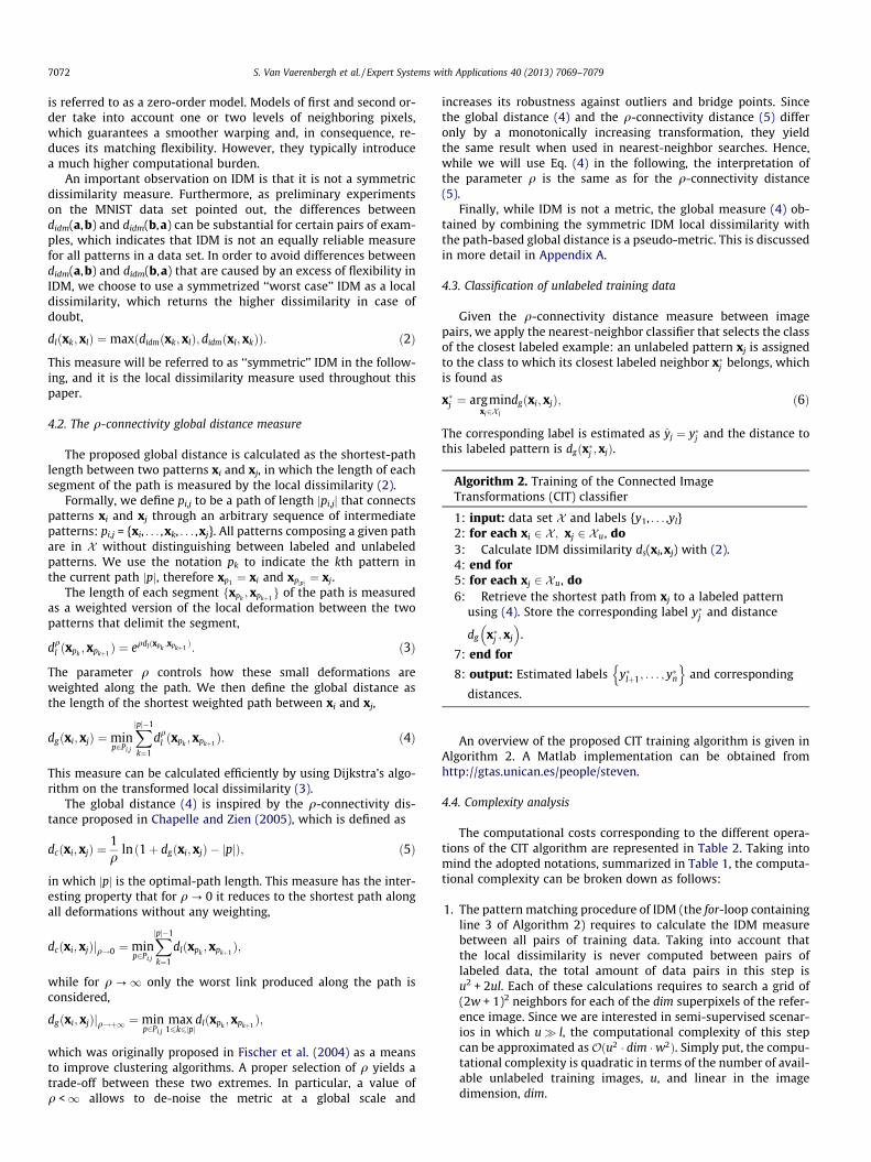
Algorithm 1. Calculation of the image distortion model (IDM)dissimilarity measure from Keysers et al. (2007). P and Qdenote the image width and height in pixels, respectively

1: input: images a and b, parameter w.2: Obtain all superpixels apq and brs of a and b.3: initialize4: d = 05: for p = 1,2, . . . ,P do6: for q = 1,2, . . . ,Q do7:

d ¼ dþmin r 2 f1; . . . ; Pg \ fp�w; . . . ; pþwgs 2 f1; . . . ;Qg \ fq�w; . . . ; qþwg

kapq � brsk2

8: end for9: end for10: output: didm(a,b) = d.

Algorithm 1 outlines the calculation of the IDM measure. Specif-ically, for each superpixel apq of image a, it aims to find the opti-mally corresponding superpixel brs of image b within a localneighborhood limited by a warp range w. The IDM dissimilarityis then calculated as the conventional Euclidean distance betweenthe superpixels of image a and the corresponding superpixels ofimage b. Since the optimal warping of one superpixel in IDM doesnot affect the optimal warping of its neighboring superpixels, IDM

7072 S. Van Vaerenbergh et al. / Expert Systems with Applications 40 (2013) 7069–7079

is referred to as a zero-order model. Models of first and second or-der take into account one or two levels of neighboring pixels,which guarantees a smoother warping and, in consequence, re-duces its matching flexibility. However, they typically introducea much higher computational burden.

An important observation on IDM is that it is not a symmetricdissimilarity measure. Furthermore, as preliminary experimentson the MNIST data set pointed out, the differences betweendidm(a,b) and didm(b,a) can be substantial for certain pairs of exam-ples, which indicates that IDM is not an equally reliable measurefor all patterns in a data set. In order to avoid differences betweendidm(a,b) and didm(b,a) that are caused by an excess of flexibility inIDM, we choose to use a symmetrized ‘‘worst case’’ IDM as a localdissimilarity, which returns the higher dissimilarity in case ofdoubt,

dlðxk;xlÞ ¼maxðdidmðxk; xlÞ;didmðxl; xkÞÞ: ð2Þ

This measure will be referred to as ‘‘symmetric’’ IDM in the follow-ing, and it is the local dissimilarity measure used throughout thispaper.

4.2. The q-connectivity global distance measure

The proposed global distance is calculated as the shortest-pathlength between two patterns xi and xj, in which the length of eachsegment of the path is measured by the local dissimilarity (2).

Formally, we define pi,j to be a path of length jpi,jj that connectspatterns xi and xj through an arbitrary sequence of intermediatepatterns: pi,j = {xi, . . . ,xk, . . . ,xj}. All patterns composing a given pathare in X without distinguishing between labeled and unlabeledpatterns. We use the notation pk to indicate the kth pattern inthe current path jpj, therefore xp1 ¼ xi and xpjpj ¼ xj.

The length of each segment fxpk;xpkþ1

g of the path is measuredas a weighted version of the local deformation between the twopatterns that delimit the segment,

dql ðxpk

;xpkþ1Þ ¼ eqdlðxpk

;xpkþ1Þ: ð3Þ

The parameter q controls how these small deformations areweighted along the path. We then define the global distance asthe length of the shortest weighted path between xi and xj,

dgðxi; xjÞ ¼minp2Pi;j

Xjpj�1

k¼1

dql ðxpk

;xpkþ1Þ: ð4Þ

This measure can be calculated efficiently by using Dijkstra’s algo-rithm on the transformed local dissimilarity (3).

The global distance (4) is inspired by the q-connectivity dis-tance proposed in Chapelle and Zien (2005), which is defined as

dcðxi;xjÞ ¼1q

ln ð1þ dgðxi;xjÞ � jpjÞ; ð5Þ

in which jpj is the optimal-path length. This measure has the inter-esting property that for q ? 0 it reduces to the shortest path alongall deformations without any weighting,

dcðxi;xjÞjq!0 ¼minp2Pi;j

Xjpj�1

k¼1

dlðxpk;xpkþ1

Þ;

while for q ?1 only the worst link produced along the path isconsidered,

dgðxi; xjÞjq!þ1 ¼minp2Pi;j

max16k6jpj

dlðxpk; xpkþ1

Þ;

which was originally proposed in Fischer et al. (2004) as a meansto improve clustering algorithms. A proper selection of q yields atrade-off between these two extremes. In particular, a value ofq <1 allows to de-noise the metric at a global scale and

increases its robustness against outliers and bridge points. Sincethe global distance (4) and the q-connectivity distance (5) differonly by a monotonically increasing transformation, they yieldthe same result when used in nearest-neighbor searches. Hence,while we will use Eq. (4) in the following, the interpretation ofthe parameter q is the same as for the q-connectivity distance(5).

Finally, while IDM is not a metric, the global measure (4) ob-tained by combining the symmetric IDM local dissimilarity withthe path-based global distance is a pseudo-metric. This is discussedin more detail in Appendix A.

4.3. Classification of unlabeled training data

Given the q-connectivity distance measure between imagepairs, we apply the nearest-neighbor classifier that selects the classof the closest labeled example: an unlabeled pattern xj is assignedto the class to which its closest labeled neighbor x�j belongs, whichis found as

x�j ¼ argminxi2X l

dgðxi; xjÞ; ð6Þ

The corresponding label is estimated as yj ¼ y�j and the distance tothis labeled pattern is dgðx�j ;xjÞ.

Algorithm 2. Training of the Connected ImageTransformations (CIT) classifier

1: input: data set X and labels {y1, . . . ,yl}2: for each xi 2 X ; xj 2 Xu, do3: Calculate IDM dissimilarity ds(xi,xj) with (2).4: end for5: for each xj 2 Xu, do6: Retrieve the shortest path from xj to a labeled pattern

using (4). Store the corresponding label y�j and distance

dg x�j ;xj

� �.

7: end for

8: output: Estimated labels y�lþ1; . . . ; y�nn o

and corresponding

distances.

An overview of the proposed CIT training algorithm is given inAlgorithm 2. A Matlab implementation can be obtained fromhttp://gtas.unican.es/people/steven.

4.4. Complexity analysis

The computational costs corresponding to the different opera-tions of the CIT algorithm are represented in Table 2. Taking intomind the adopted notations, summarized in Table 1, the computa-tional complexity can be broken down as follows:

1. The pattern matching procedure of IDM (the for-loop containingline 3 of Algorithm 2) requires to calculate the IDM measurebetween all pairs of training data. Taking into account thatthe local dissimilarity is never computed between pairs oflabeled data, the total amount of data pairs in this step isu2 + 2ul. Each of these calculations requires to search a grid of(2w + 1)2 neighbors for each of the dim superpixels of the refer-ence image. Since we are interested in semi-supervised scenar-ios in which u� l, the computational complexity of this stepcan be approximated asOðu2 � dim �w2Þ. Simply put, the compu-tational complexity is quadratic in terms of the number of avail-able unlabeled training images, u, and linear in the imagedimension, dim.

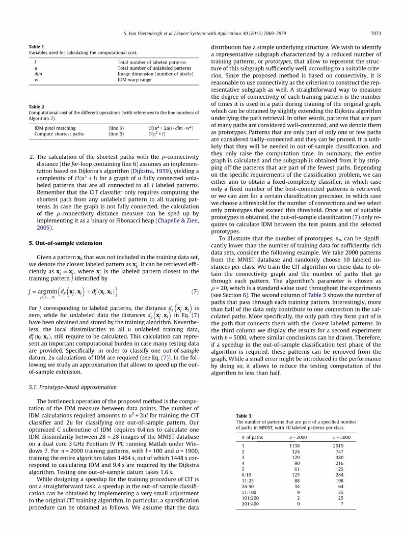
Table 3The number of patterns that are part of a specified numberof paths in MNIST, with 10 labeled patterns per class.

# of paths n = 2000 n = 5000

1 1138 29192 324 7473 129 3804 90 2165 61 1256:10 125 28411:25 88 19826:50 34 6451:100 9 35101:200 2 25201:400 0 7

Table 1Variables used for calculating the computational cost.

l Total number of labeled patternsu Total number of unlabeled patternsdim Image dimension (number of pixels)w IDM warp range

Table 2Computational cost of the different operations (with references to the line numbers ofAlgorithm 2).

IDM pixel matching (line 3) O((u2 + 2ul) � dim � w2)Compute shortest paths (line 6) O(u2 + l)

S. Van Vaerenbergh et al. / Expert Systems with Applications 40 (2013) 7069–7079 7073

2. The calculation of the shortest paths with the q-connectivitydistance (the for-loop containing line 6) assumes an implemen-tation based on Dijkstra’s algorithm (Dijkstra, 1959), yielding acomplexity of Oðu2 þ lÞ for a graph of u fully connected unla-beled patterns that are all connected to all l labeled patterns.Remember that the CIT classifier only requires computing theshortest path from any unlabeled pattern to all training pat-terns. In case the graph is not fully connected, the calculationof the q-connectivity distance measure can be sped up byimplementing it as a binary or Fibonacci heap (Chapelle & Zien,2005).

5. Out-of-sample extension

Given a pattern xk that was not included in the training data set,we denote the closest labeled pattern as x�k. It can be retrieved effi-ciently as x�k ¼ x�j , where x�j is the labeled pattern closest to thetraining pattern j identified by

j ¼ argminj2½1;...;n�

dg x�j ; xj

� �þ dq

l ðxj;xkÞ� �

: ð7Þ

For j corresponding to labeled patterns, the distance dg x�j ;xj

� �is

zero, while for unlabeled data the distances dg x�j ;xj

� �in Eq. (7)

have been obtained and stored by the training algorithm. Neverthe-less, the local dissimilarities to all u unlabeled training data,dq

l ðxj;xkÞ, still require to be calculated. This calculation can repre-sent an important computational burden in case many testing dataare provided. Specifically, in order to classify one out-of-sampledatum, 2u calculations of IDM are required (see Eq. (7)). In the fol-lowing we study an approximation that allows to speed up the out-of-sample extension.

5.1. Prototype-based approximation

The bottleneck operation of the proposed method is the compu-tation of the IDM measure between data points. The number ofIDM calculations required amounts to u2 + 2ul for training the CITclassifier and 2u for classifying one out-of-sample pattern. Ouroptimized C subroutine of IDM requires 0.4 ms to calculate oneIDM dissimilarity between 28 � 28 images of the MNIST databaseon a dual core 3 GHz Pentium IV PC running Matlab under Win-dows 7. For n = 2000 training patterns, with l = 100 and u = 1900,training the entire algorithm takes 1464 s, out of which 1448 s cor-respond to calculating IDM and 9.4 s are required by the Dijkstraalgorithm. Testing one out-of-sample datum takes 1.6 s.

While designing a speedup for the training procedure of CIT isnot a straightforward task, a speedup in the out-of-sample classifi-cation can be obtained by implementing a very small adjustmentto the original CIT training algorithm. In particular, a sparsificationprocedure can be obtained as follows. We assume that the data

distribution has a simple underlying structure. We wish to identifya representative subgraph characterized by a reduced number oftraining patterns, or prototypes, that allow to represent the struc-ture of this subgraph sufficiently well, according to a suitable crite-rion. Since the proposed method is based on connectivity, it isreasonable to use connectivity as the criterion to construct the rep-resentative subgraph as well. A straightforward way to measurethe degree of connectivity of each training pattern is the numberof times it is used in a path during training of the original graph,which can be obtained by slightly extending the Dijkstra algorithmunderlying the path retrieval. In other words, patterns that are partof many paths are considered well-connected, and we denote themas prototypes. Patterns that are only part of only one or few pathsare considered badly-connected and they can be pruned. It is unli-kely that they will be needed in out-of-sample classification, andthey only raise the computation time. In summary, the entiregraph is calculated and the subgraph is obtained from it by strip-ping off the patterns that are part of the fewest paths. Dependingon the specific requirements of the classification problem, we caneither aim to obtain a fixed-complexity classifier, in which caseonly a fixed number of the best-connected patterns is retrieved,or we can aim for a certain classification precision, in which casewe choose a threshold for the number of connections and we selectonly prototypes that exceed this threshold. Once a set of suitableprototypes is obtained, the out-of-sample classification (7) only re-quires to calculate IDM between the test points and the selectedprototypes.

To illustrate that the number of prototypes, np, can be signifi-cantly lower than the number of training data for sufficiently richdata sets, consider the following example. We take 2000 patternsfrom the MNIST database and randomly choose 10 labeled in-stances per class. We train the CIT algorithm on these data to ob-tain the connectivity graph and the number of paths that gothrough each pattern. The algorithm’s parameter is chosen asq = 20, which is a standard value used throughout the experiments(see Section 6). The second column of Table 3 shows the number ofpaths that pass through each training pattern. Interestingly, morethan half of the data only contribute to one connection in the cal-culated paths. More specifically, the only path they form part of isthe path that connects them with the closest labeled patterns. Inthe third column we display the results for a second experimentwith n = 5000, where similar conclusions can be drawn. Therefore,if a speedup in the out-of-sample classification test phase of thealgorithm is required, these patterns can be removed from thegraph. While a small error might be introduced in the performanceby doing so, it allows to reduce the testing computation of thealgorithm to less than half.

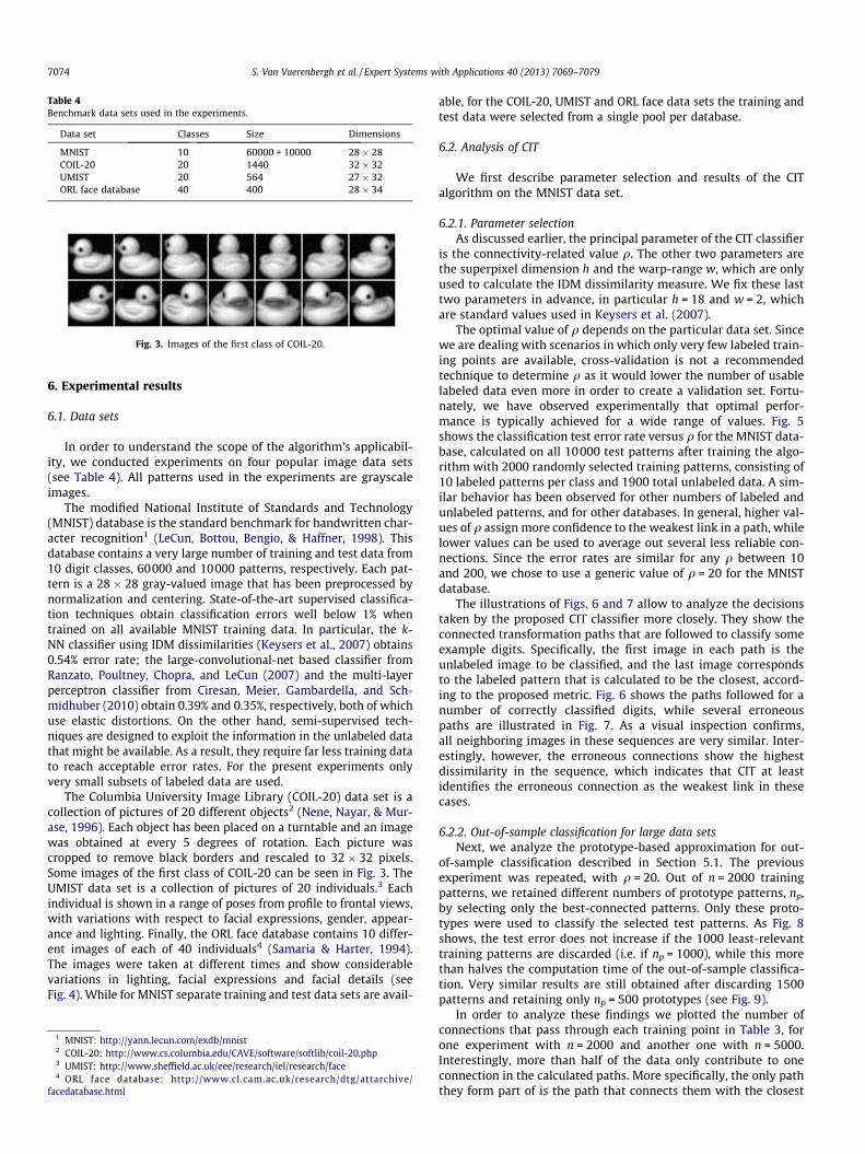
Table 4Benchmark data sets used in the experiments.

Data set Classes Size Dimensions

MNIST 10 60000 + 10000 28 � 28COIL-20 20 1440 32 � 32UMIST 20 564 27 � 32ORL face database 40 400 28 � 34

Fig. 3. Images of the first class of COIL-20.

7074 S. Van Vaerenbergh et al. / Expert Systems with Applications 40 (2013) 7069–7079

6. Experimental results

6.1. Data sets

In order to understand the scope of the algorithm’s applicabil-ity, we conducted experiments on four popular image data sets(see Table 4). All patterns used in the experiments are grayscaleimages.

The modified National Institute of Standards and Technology(MNIST) database is the standard benchmark for handwritten char-acter recognition1 (LeCun, Bottou, Bengio, & Haffner, 1998). Thisdatabase contains a very large number of training and test data from10 digit classes, 60000 and 10000 patterns, respectively. Each pat-tern is a 28 � 28 gray-valued image that has been preprocessed bynormalization and centering. State-of-the-art supervised classifica-tion techniques obtain classification errors well below 1% whentrained on all available MNIST training data. In particular, the k-NN classifier using IDM dissimilarities (Keysers et al., 2007) obtains0.54% error rate; the large-convolutional-net based classifier fromRanzato, Poultney, Chopra, and LeCun (2007) and the multi-layerperceptron classifier from Ciresan, Meier, Gambardella, and Sch-midhuber (2010) obtain 0.39% and 0.35%, respectively, both of whichuse elastic distortions. On the other hand, semi-supervised tech-niques are designed to exploit the information in the unlabeled datathat might be available. As a result, they require far less training datato reach acceptable error rates. For the present experiments onlyvery small subsets of labeled data are used.

The Columbia University Image Library (COIL-20) data set is acollection of pictures of 20 different objects2 (Nene, Nayar, & Mur-ase, 1996). Each object has been placed on a turntable and an imagewas obtained at every 5 degrees of rotation. Each picture wascropped to remove black borders and rescaled to 32 � 32 pixels.Some images of the first class of COIL-20 can be seen in Fig. 3. TheUMIST data set is a collection of pictures of 20 individuals.3 Eachindividual is shown in a range of poses from profile to frontal views,with variations with respect to facial expressions, gender, appear-ance and lighting. Finally, the ORL face database contains 10 differ-ent images of each of 40 individuals4 (Samaria & Harter, 1994).The images were taken at different times and show considerablevariations in lighting, facial expressions and facial details (seeFig. 4). While for MNIST separate training and test data sets are avail-

1 MNIST: http://yann.lecun.com/exdb/mnist2 COIL-20: http://www.cs.columbia.edu/CAVE/software/softlib/coil-20.php3 UMIST: http://www.sheffield.ac.uk/eee/research/iel/research/face4 ORL face database: http://www.cl.cam.ac.uk/research/dtg/attarchive/

facedatabase.html

able, for the COIL-20, UMIST and ORL face data sets the training andtest data were selected from a single pool per database.

6.2. Analysis of CIT

We first describe parameter selection and results of the CITalgorithm on the MNIST data set.

6.2.1. Parameter selectionAs discussed earlier, the principal parameter of the CIT classifier

is the connectivity-related value q. The other two parameters arethe superpixel dimension h and the warp-range w, which are onlyused to calculate the IDM dissimilarity measure. We fix these lasttwo parameters in advance, in particular h = 18 and w = 2, whichare standard values used in Keysers et al. (2007).

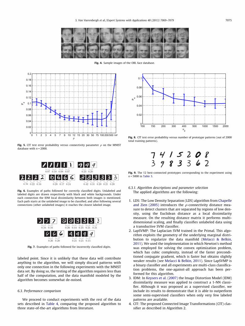
The optimal value of q depends on the particular data set. Sincewe are dealing with scenarios in which only very few labeled train-ing points are available, cross-validation is not a recommendedtechnique to determine q as it would lower the number of usablelabeled data even more in order to create a validation set. Fortu-nately, we have observed experimentally that optimal perfor-mance is typically achieved for a wide range of values. Fig. 5shows the classification test error rate versus q for the MNIST data-base, calculated on all 10000 test patterns after training the algo-rithm with 2000 randomly selected training patterns, consisting of10 labeled patterns per class and 1900 total unlabeled data. A sim-ilar behavior has been observed for other numbers of labeled andunlabeled patterns, and for other databases. In general, higher val-ues of q assign more confidence to the weakest link in a path, whilelower values can be used to average out several less reliable con-nections. Since the error rates are similar for any q between 10and 200, we chose to use a generic value of q = 20 for the MNISTdatabase.

The illustrations of Figs. 6 and 7 allow to analyze the decisionstaken by the proposed CIT classifier more closely. They show theconnected transformation paths that are followed to classify someexample digits. Specifically, the first image in each path is theunlabeled image to be classified, and the last image correspondsto the labeled pattern that is calculated to be the closest, accord-ing to the proposed metric. Fig. 6 shows the paths followed for anumber of correctly classified digits, while several erroneouspaths are illustrated in Fig. 7. As a visual inspection confirms,all neighboring images in these sequences are very similar. Inter-estingly, however, the erroneous connections show the highestdissimilarity in the sequence, which indicates that CIT at leastidentifies the erroneous connection as the weakest link in thesecases.

6.2.2. Out-of-sample classification for large data setsNext, we analyze the prototype-based approximation for out-

of-sample classification described in Section 5.1. The previousexperiment was repeated, with q = 20. Out of n = 2000 trainingpatterns, we retained different numbers of prototype patterns, np,by selecting only the best-connected patterns. Only these proto-types were used to classify the selected test patterns. As Fig. 8shows, the test error does not increase if the 1000 least-relevanttraining patterns are discarded (i.e. if np = 1000), while this morethan halves the computation time of the out-of-sample classifica-tion. Very similar results are still obtained after discarding 1500patterns and retaining only np = 500 prototypes (see Fig. 9).

In order to analyze these findings we plotted the number ofconnections that pass through each training point in Table 3, forone experiment with n = 2000 and another one with n = 5000.Interestingly, more than half of the data only contribute to oneconnection in the calculated paths. More specifically, the only paththey form part of is the path that connects them with the closest

0 1 2 3 4 5 7 9 10 12 15 20 30 50 75 100 200500 Inf0

0.02

0.04

0.06

0.08

0.1

0.12

0.14

0.16

0.18

0.2

ρ

P e

Fig. 5. CIT test error probability versus connectivity parameter q on the MNISTdatabase with n = 2000.

Fig. 4. Sample images of the ORL face database.

100 150 200 300 400 500 1000 1500 20000

0.02

0.04

0.06

0.08

0.1

npP e

Fig. 8. CIT test error probability versus number of prototype patterns (out of 2000total training patterns).

Fig. 6. Examples of paths followed for correctly classified digits. Unlabeled andlabeled digits are drawn respectively with black and white backgrounds. Undereach connection the IDM local dissimilarity between both images is mentioned.Each path starts at the unlabeled image to be classified, and after following severalconnections (other unlabeled images) it reaches the closest labeled image.

Fig. 7. Examples of paths followed for incorrectly classified digits.

Fig. 9. The 12 best-connected prototypes corresponding to the experiment usingn = 5000 in Table 3.

S. Van Vaerenbergh et al. / Expert Systems with Applications 40 (2013) 7069–7079 7075

labeled point. Since it is unlikely that these data will contributeanything to the algorithm, we will simply discard patterns withonly one connection in the following experiments with the MNISTdata set. By doing so, the testing of the algorithm requires less thanhalf of the computation, and the data manifold modeled by thealgorithm becomes somewhat de-noised.

6.3. Performance comparison

We proceed to conduct experiments with the rest of the datasets described in Table 4, comparing the proposed algorithm tothree state-of-the-art algorithms from literature.

6.3.1. Algorithm descriptions and parameter selectionThe applied algorithms are the following:

1. LDS: The Low Density Separation (LDS) algorithm from Chapelleand Zien (2005) introduces the q-connectivity distance mea-sure to detect clusters that are separated by regions of low den-sity, using the Euclidean distance as a local dissimilaritymeasure. On the resulting distance matrix it performs multi-dimensional scaling, and finally classifies unlabeled data usinga transductive SVM classifier.

2. LapSVMP: The Laplacian SVM trained in the Primal. This algo-rithm exploits the geometry of the underlying marginal distri-bution to regularize the data manifold (Melacci & Belkin,2011). We used the implementation in which Newton’s methodwas employed for solving the convex optimization problem,which has cubic complexity, instead of the faster precondi-tioned conjugate gradient, which is faster but obtains slightlyweaker results (see Melacci & Belkin, 2011). Since LapSVMP isa binary classifier and all experiments are multi-class classifica-tion problems, the one-against-all approach has been per-formed for this algorithm.

3. IDM: In Keysers et al. (2007) the Image Distortion Model (IDM)dissimilarity measure was applied to construct a 1-NN classi-fier. Although it was proposed as a supervised classifier, weinclude its results to demonstrate that it is able to outperformsome semi-supervised classifiers when only very few labeledpatterns are available.

4. CIT: The proposed Connected Image Transformations (CIT) clas-sifier as described in Algorithm 2.

250 500 750 1000 2000 3000 4000 500010−2

10−1

Number of training data

P e

LDSLapSVMPIDMCIT

Fig. 10. Error probabilities on the unlabeled training data, for different numbers oftotal training data n.

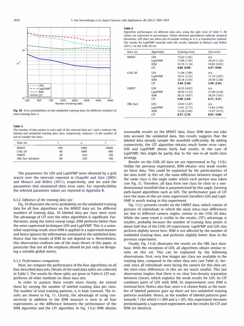
Table 5The number of data points in each split of the selected data set. l and u indicate thelabeled and unlabeled training data sizes, respectively, whereas t is the number ofout-of-sample test data.

Data set l u t

MNIST 100 1900 10000COIL-20 40 1000 400UMIST 40 424 100ORL face database 80 220 100

Table 6Algorithm performance on different data sets, using the split sizes of Table 5. Allvalues are expressed in percentages. Values between parentheses indicate standarddeviations. LDS does not allow out-of-sample testing as it is a transductive method.The results for LapSVMP coincide with the results reported in Melacci and Belkin(2011), on the COIL-20 set.

Data set Algorithm Training error Test error

MNIST LDS 15.62 (1.82) n/aLapSVMP 17.89 (1.92) 19.24 (1.22)IDM 10.76 (1.14) 10.02 (0.93)CIT 4.86 (0.98) 4.57 (0.96)

COIL-20 LDS 11.04 (1.89) n/aLapSVMP 10.31 (2.32) 11.79 (2.87)IDM 24.18 (1.93) 24.50 (2.40)CIT 3.44 (2.20) 3.49 (2.45)

UMIST LDS 16.53 (4.03) n/aLapSVMP 20.56 (3.32) 21.00 (4.26)IDM 38.21 (4.07) 38.29 (5.81)CIT 5.90 (2.45) 6.11 (3.31)

ORL face LDS 14.92 (3.47) n/aLapSVMP 13.61 (2.73) 13.82 (3.99)IDM 12.20 (2.66) 12.97 (4.15)CIT 8.57 (2.76) 8.91 (3.08)

7076 S. Van Vaerenbergh et al. / Expert Systems with Applications 40 (2013) 7069–7079

The parameters for LDS and LapSVMP were obtained by a gridsearch over the intervals reported in Chapelle and Zien (2005)and Melacci and Belkin (2011), respectively, and we used theparameters that minimized their error rates. For reproducibilitythe selected parameter values are reported in Appendix B.

6.3.2. Influence of the training data sizeFig. 10 illustrates the error probability on the unlabeled training

data for all four algorithms on the MNIST data set, for differentnumbers of training data. 10 labeled data per class were used.The advantage of CIT over the other algorithms is significant. Fur-thermore, along the entire sweep range, IDM performs better thanthe semi-supervised techniques LDS and LapSVMP. This is a some-what surprising result, since IDM is applied in a supervised mannerand hence ignores the information contained in the unlabeled data.Notice that the results of IDM do not depend on n. Nevertheless,this observation confirms one of the main theses of this paper, inparticular that not all the emphasis should be put only on design-ing a suitable global metric.

6.3.3. Performance comparisonNext, we compare the performance of the four algorithms on all

four described data sets. Details of the used data splits are collectedin Table 5. The results for these splits are given in Table 6. CIT out-performs all other methods on these data sets.

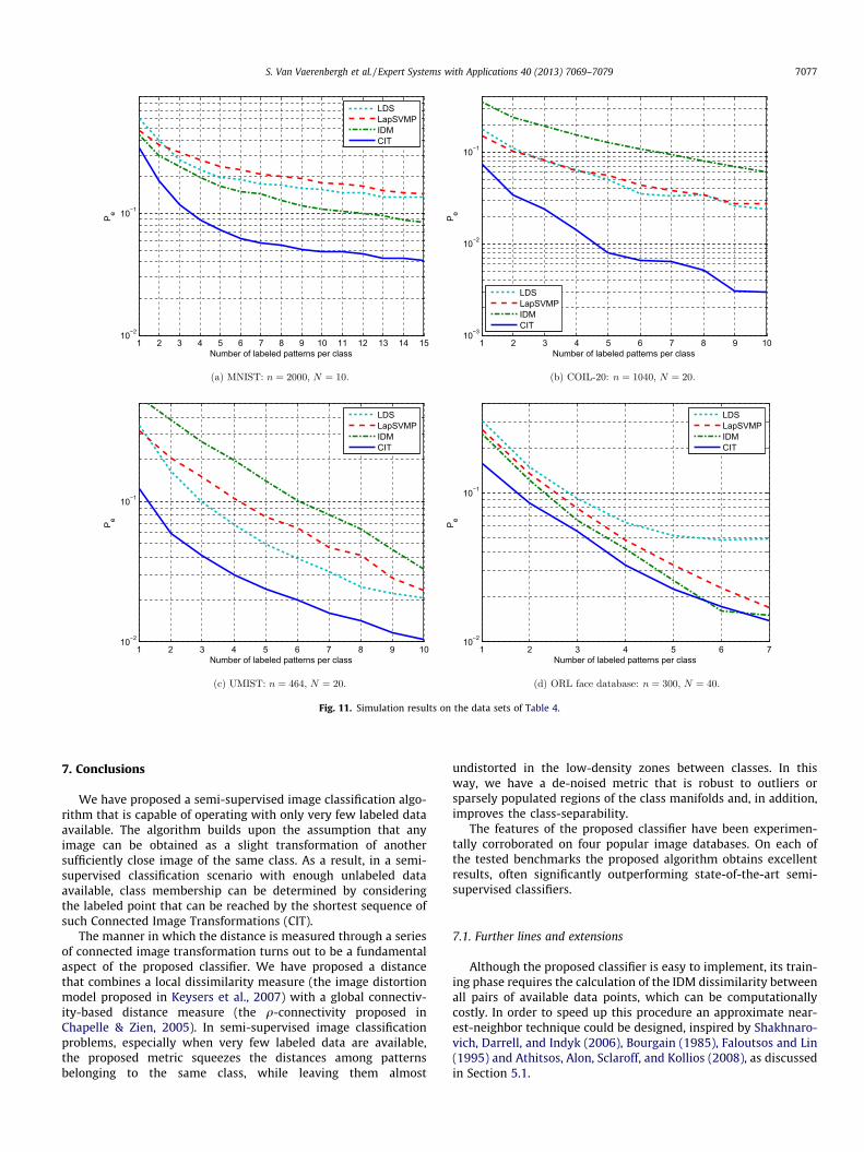
In order to analyze these results more closely, we extendthem by varying the number of labeled training data per class.The number of total training patterns, n, is kept constant. The re-sults are shown in Fig. 11. Clearly, the advantage of using con-nectivity in addition to the IDM measure is seen in all fourexperiments as the difference between the performance of theIDM algorithm and the CIT algorithm. In Fig. 11(a) IDM obtains

reasonable results on the MNIST data. Since IDM does not takeinto account the unlabeled data, this results suggests that thelabeled data already sample the manifold sufficiently. By addingconnectivity, the CIT algorithm obtains much lower error rates.LDS and LapSVMP obtain fairly bad results. In the case ofLapSVMP, this might be partly due to the one-vs-all multi-classstrategy.

Results on the COIL-20 data set are represented in Fig. 11(b).Unlike the previous experiment, IDM obtains very weak resultson these data. This could be explained by the particularities ofthe data itself: in this set, the main difference between images ofthe same class is the angle under which each picture was taken(see Fig. 3). Therefore, all data from one class lie close to a one-dimensional manifold that is parameterized by this angle, favoringpath-based algorithms such as LDS. The performance gain of CITover the state-of-the-art semi-supervised classifiers LDS and LapS-VMP is worth noting in this experiment.

Fig. 11(c) presents results on the UMIST data, which consist ofpictures of individuals in which the main intra-class differencesare due to different camera angles, similar to the COIL-20 data.While the same trend is visible in the results, CIT’s advantage issmaller, probably because the number of training data points isabout half that of the COIL-20 experiment. LapSVMP and LDS alsoperform slightly worse here. IDM is not affected by the number ofunlabeled training data, and performs slightly better than in theprevious experiment.

Finally, Fig. 11(d) illustrates the results on the ORL face data-base. With the exception of LDS, all algorithms obtain similar re-sults on this set. This can be explained by the followingobservations. First, very few images per class are available in thetraining data, compared to the other data sets (see Table 4). Sec-ond, since all individuals were facing the camera for this data set,the inter-class differences in this set are much smaller. This lastobservation implies that there is no clear low-density separationbetween classes, which explains the weak results for LDS. As CITcombines parts of LDS with IDM, its improvement over IDM isminimal here. Notice also that, since n is chosen fixed, as the num-ber of labeled patterns goes up there are less unlabeled trainingpatterns available. Hence, as the number of labeled patterns goestowards 7 (for which l = 280 and u = 20), this experiment becomespredominantly a supervised experiment and the results for CIT andIDM are identical.

1 2 3 4 5 6 7 8 9 10 11 12 13 14 1510−2

10−1

Number of labeled patterns per class

P eLDSLapSVMPIDMCIT

1 2 3 4 5 6 7 8 9 1010−3

10−2

10−1

Number of labeled patterns per class

P e

LDSLapSVMPIDMCIT

1 2 3 4 5 6 7 8 9 1010−2

10−1

Number of labeled patterns per class

P e

LDSLapSVMPIDMCIT

1 2 3 4 5 6 710−2

10−1

Number of labeled patterns per class

P e

LDSLapSVMPIDMCIT

Fig. 11. Simulation results on the data sets of Table 4.

S. Van Vaerenbergh et al. / Expert Systems with Applications 40 (2013) 7069–7079 7077

7. Conclusions

We have proposed a semi-supervised image classification algo-rithm that is capable of operating with only very few labeled dataavailable. The algorithm builds upon the assumption that anyimage can be obtained as a slight transformation of anothersufficiently close image of the same class. As a result, in a semi-supervised classification scenario with enough unlabeled dataavailable, class membership can be determined by consideringthe labeled point that can be reached by the shortest sequence ofsuch Connected Image Transformations (CIT).

The manner in which the distance is measured through a seriesof connected image transformation turns out to be a fundamentalaspect of the proposed classifier. We have proposed a distancethat combines a local dissimilarity measure (the image distortionmodel proposed in Keysers et al., 2007) with a global connectiv-ity-based distance measure (the q-connectivity proposed inChapelle & Zien, 2005). In semi-supervised image classificationproblems, especially when very few labeled data are available,the proposed metric squeezes the distances among patternsbelonging to the same class, while leaving them almost

undistorted in the low-density zones between classes. In thisway, we have a de-noised metric that is robust to outliers orsparsely populated regions of the class manifolds and, in addition,improves the class-separability.

The features of the proposed classifier have been experimen-tally corroborated on four popular image databases. On each ofthe tested benchmarks the proposed algorithm obtains excellentresults, often significantly outperforming state-of-the-art semi-supervised classifiers.

7.1. Further lines and extensions

Although the proposed classifier is easy to implement, its train-ing phase requires the calculation of the IDM dissimilarity betweenall pairs of available data points, which can be computationallycostly. In order to speed up this procedure an approximate near-est-neighbor technique could be designed, inspired by Shakhnaro-vich, Darrell, and Indyk (2006), Bourgain (1985), Faloutsos and Lin(1995) and Athitsos, Alon, Sclaroff, and Kollios (2008), as discussedin Section 5.1.

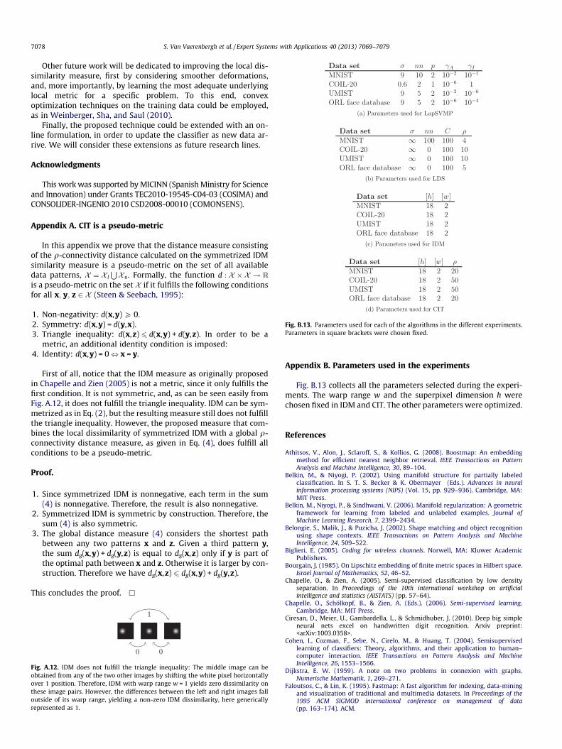
Fig. B.13. Parameters used for each of the algorithms in the different experiments.Parameters in square brackets were chosen fixed.

7078 S. Van Vaerenbergh et al. / Expert Systems with Applications 40 (2013) 7069–7079

Other future work will be dedicated to improving the local dis-similarity measure, first by considering smoother deformations,and, more importantly, by learning the most adequate underlyinglocal metric for a specific problem. To this end, convexoptimization techniques on the training data could be employed,as in Weinberger, Sha, and Saul (2010).

Finally, the proposed technique could be extended with an on-line formulation, in order to update the classifier as new data ar-rive. We will consider these extensions as future research lines.

Acknowledgments

This work was supported by MICINN (Spanish Ministry for Scienceand Innovation) under Grants TEC2010-19545-C04-03 (COSIMA) andCONSOLIDER-INGENIO 2010 CSD2008-00010 (COMONSENS).

Appendix A. CIT is a pseudo-metric

In this appendix we prove that the distance measure consistingof the q-connectivity distance calculated on the symmetrized IDMsimilarity measure is a pseudo-metric on the set of all availabledata patterns, X ¼ X l

SXu. Formally, the function d : X � X ! R

is a pseudo-metric on the set X if it fulfills the following conditionsfor all x; y; z 2 X (Steen & Seebach, 1995):

1. Non-negativity: d(x,y) P 0.2. Symmetry: d(x,y) = d(y,x).3. Triangle inequality: d(x,z) 6 d(x,y) + d(y,z). In order to be a

metric, an additional identity condition is imposed:4. Identity: d(x,y) = 0, x = y.

First of all, notice that the IDM measure as originally proposedin Chapelle and Zien (2005) is not a metric, since it only fulfills thefirst condition. It is not symmetric, and, as can be seen easily fromFig. A.12, it does not fulfill the triangle inequality. IDM can be sym-metrized as in Eq. (2), but the resulting measure still does not fulfillthe triangle inequality. However, the proposed measure that com-bines the local dissimilarity of symmetrized IDM with a global q-connectivity distance measure, as given in Eq. (4), does fulfill allconditions to be a pseudo-metric.

Proof.

1. Since symmetrized IDM is nonnegative, each term in the sum(4) is nonnegative. Therefore, the result is also nonnegative.

2. Symmetrized IDM is symmetric by construction. Therefore, thesum (4) is also symmetric.

3. The global distance measure (4) considers the shortest pathbetween any two patterns x and z. Given a third pattern y,the sum dg(x,y) + dg(y,z) is equal to dg(x,z) only if y is part ofthe optimal path between x and z. Otherwise it is larger by con-struction. Therefore we have dg(x,z) 6 dg(x,y) + dg(y,z).

This concludes the proof. h

Fig. A.12. IDM does not fulfill the triangle inequality: The middle image can beobtained from any of the two other images by shifting the white pixel horizontallyover 1 position. Therefore, IDM with warp range w = 1 yields zero dissimilarity onthese image pairs. However, the differences between the left and right images falloutside of its warp range, yielding a non-zero IDM dissimilarity, here genericallyrepresented as 1.

Appendix B. Parameters used in the experiments

Fig. B.13 collects all the parameters selected during the experi-ments. The warp range w and the superpixel dimension h werechosen fixed in IDM and CIT. The other parameters were optimized.

References

Athitsos, V., Alon, J., Sclaroff, S., & Kollios, G. (2008). Boostmap: An embeddingmethod for efficient nearest neighbor retrieval. IEEE Transactions on PatternAnalysis and Machine Intelligence, 30, 89–104.

Belkin, M., & Niyogi, P. (2002). Using manifold structure for partially labeledclassification. In S. T. S. Becker & K. Obermayer (Eds.). Advances in neuralinformation processing systems (NIPS) (Vol. 15, pp. 929–936). Cambridge, MA:MIT Press.

Belkin, M., Niyogi, P., & Sindhwani, V. (2006). Manifold regularization: A geometricframework for learning from labeled and unlabeled examples. Journal ofMachine Learning Research, 7, 2399–2434.

Belongie, S., Malik, J., & Puzicha, J. (2002). Shape matching and object recognitionusing shape contexts. IEEE Transactions on Pattern Analysis and MachineIntelligence, 24, 509–522.

Biglieri, E. (2005). Coding for wireless channels. Norwell, MA: Kluwer AcademicPublishers.

Bourgain, J. (1985). On Lipschitz embedding of finite metric spaces in Hilbert space.Israel Journal of Mathematics, 52, 46–52.

Chapelle, O., & Zien, A. (2005). Semi-supervised classification by low densityseparation. In Proceedings of the 10th international workshop on artificialintelligence and statistics (AISTATS) (pp. 57–64).

Chapelle, O., Schölkopf, B., & Zien, A. (Eds.). (2006). Semi-supervised learning.Cambridge, MA: MIT Press.

Ciresan, D., Meier, U., Gambardella, L., & Schmidhuber, J. (2010). Deep big simpleneural nets excel on handwritten digit recognition. Arxiv preprint:<arXiv:1003.0358>.

Cohen, I., Cozman, F., Sebe, N., Cirelo, M., & Huang, T. (2004). Semisupervisedlearning of classifiers: Theory, algorithms, and their application to human–computer interaction. IEEE Transactions on Pattern Analysis and MachineIntelligence, 26, 1553–1566.

Dijkstra, E. W. (1959). A note on two problems in connexion with graphs.Numerische Mathematik, 1, 269–271.

Faloutsos, C., & Lin, K. (1995). Fastmap: A fast algorithm for indexing, data-miningand visualization of traditional and multimedia datasets. In Proceedings of the1995 ACM SIGMOD international conference on management of data(pp. 163–174). ACM.

S. Van Vaerenbergh et al. / Expert Systems with Applications 40 (2013) 7069–7079 7079

Fischer, B., Roth, V., & Buhmann, J. M. (2004). Clustering with the connectivitykernel. In S. Thrun, L. Saul, & B. Schölkopf (Eds.). Advances in neural informationprocessing systems (NIPS) (Vol. 16, pp. 89–96). Cambridge, MA: MIT Press.

Francois, D., Wertz, V., & Verleysen, M. (2007). The concentration of fractionaldistances. IEEE Transactions on Knowledge and Data Engineering, 19, 873–886.

Jaakkola, T. S., & Szummer, M. (2002). Partially labeled classification with markovrandom walks. In T. G. Dietterich, S. Becker, & Z. Ghahramani (Eds.). Advances inneural information processing systems (NIPS) (Vol. 14, pp. 945–952). Cambridge,MA: MIT Press.

Joachims, T. (1998). Text categorization with support vector machines: Learningwith many relevant features. In European conference on machine learning (ECML)(pp. 137–142). Berlin: Springer.

Keysers, D., Deselaers, T., Gollan, C., & Ney, H. (2007). Deformation models for imagerecognition. IEEE Transactions on Pattern Analysis and Machine Intelligence, 29,1422–1435.

LeCun, Y., Bottou, L., Bengio, Y., & Haffner, P. (1998). Gradient-based learningapplied to document recognition. Proceedings of the IEEE, 86, 2278–2324.

Melacci, S., & Belkin, M. (2011). Laplacian support vector machines trained in theprimal. Journal of Machine Learning Research, 12, 1149–1184.

Nene, S. A., Nayar, S. K., & Murase, H. (1996). Columbia object image library (COIL-20). Technical report CUCS-005-96, Department of Computer Science, ColumbiaUniversity, New York.

Rajan, S., Ghosh, J., & Crawford, M. (2008). An active learning approach tohyperspectral data classification. IEEE Transactions on Geoscience and RemoteSensing, 46, 1231–1242.

Ranzato, M., Poultney, C., Chopra, S., & LeCun, Y. (2007). Efficient learning of sparserepresentations with an energy-based model. In B. Schölkopf, J. Platt, & T.Hoffman (Eds.). Advances in neural information processing systems (NIPS) (Vol.19, pp. 1137–1144). Cambridge, MA: MIT Press.

Samaria, F., & Harter, A. (1994). Parameterisation of a stochastic model for humanface identification. In Proceedings of the second IEEE workshop on applications ofcomputer vision (pp. 138–142).

Shakhnarovich, G., Darrell, T., & Indyk, P. (2006). Nearest-neighbor methods inlearning and vision: Theory and practice. The MIT Press.

Steen, L., & Seebach, J. (1995). Counterexamples in topology. Courier DoverPublications.

Szlam, A. D., Maggioni, M., & Coifman, R. R. (2008). Regularization on graphs withfunction-adapted diffusion processes. Journal of Machine Learning Research, 9,1711–1739.

Uchida, S., & Sakoe, H. (2003). Eigen-deformations for elastic matching basedhandwritten recognition. Pattern Recognition, 36, 2031–2040.

Van Vaerenbergh, S., Santamaría, I., & Barbano, P.E. (2011). Semi-supervisedhandwritten digit recognition using very few labeled data. In IEEEinternational conference on acoustics, speech, and signal processing (ICASSP) (pp.2136–2139). Prague, Czech Republic.

Wang, F., & Zhang, C. (2007). Robust self-tuning semi-supervised learning.Neurocomputing, 70, 2931–2939.

Weinberger, K. Q., Sha, F., & Saul, L. K. (2010). Convex optimizations for distancemetric learning and pattern classification. IEEE Signal Processing Magazine, 27,146–158.

Weston, J., Leslie, C., Zhou, D., Elisseeff, A., & Noble, W. S. (2004). Semi-supervisedprotein classification using cluster kernels. In S. Thrun, L. Saul, & B. Schölkopf(Eds.). Advances in neural information processing systems (NIPS) (Vol. 16,pp. 3241–3247). Cambridge, MA: MIT Press.

Zhou, D., Bousquet, O., Lal, T. N., Weston, J., & Schölkopf, B. (2004). Learning withlocal and global consistency. In S. Thrun, L. Saul, & B. Schölkopf (Eds.). Advancesin neural information processing systems (NIPS) (Vol. 16, pp. 321–328).Cambridge, MA: MIT Press.

Zhu, X. (2005). Semi-supervised learning literature survey. Technical report 1530,Computer Sciences, University of Wisconsin-Madison.

Zhu, X., Ghahramani, Z., & Lafferty, J. (2003). Semi-supervised learning usingGaussian fields and harmonic functions. In Proceedings of the 20th internationalconference on machine learning (ICML) (pp. 912–919). Washington, DC, USA.