Semi-Parametric Models for the Multivariate TailDependence Function - the Asymptotically

Dependent Case

By CLAUDIA KLUPPELBERG, GABRIEL KUHN

Center for Mathematical Sciences, Munich University of Technology, D-85747 Garching,

Germany.

cklu@ma.tum.de gabriel@ma.tum.de

and LIANG PENG

School of Mathematics, Georgia Institute of Technology, Atlanta, GA 30332-0160, USA.

peng@math.gatech.edu

Summary

In general, the risk of joint extreme outcomes in financial markets can be expressed as

a function of the tail dependence function of a high-dimensional vector after standardizing

marginals. Hence it is of importance to model and estimate tail dependence functions.

Even for moderate dimension, nonparametrically estimating a tail dependence function is

very inefficient and fitting a parametric model to tail dependence functions is not robust.

In this paper we propose a semi-parametric model for (asymptotically dependent) tail

dependence functions via an elliptical copula. Based on this model assumption, we propose

a novel estimator for the tail dependence function, which proves favorable compared to

the empirical tail dependence function estimator, both theoretically and empirically.

Keywords: Asymptotic normality, Dependence modeling, Elliptical copula, Elliptical distribu-

tion, Regular variation, Semi-parametric model, Tail dependence function.

1 Introduction

Risk management is a discipline for living with the possibility that future events may cause

adverse effects. An important issue for risk managers is how to quantify different types of

risk such as market risk, credit risk, operational risk, etc. Due to the multivariate nature

of risk, i.e., risk depending on high dimensional vectors of some underlying risk factors, a

particular concern for a risk manager is how to model the dependence between extreme

outcomes although those extreme outcomes occur rarely. A mathematical formulation of

this question is as follows. Let X = (X1, . . . , Xd)T be a random vector with distribution

function F and continuous marginals F1, . . . , Fd. Then the dependence is completely de-

termined by the copula C of X given by Sklar’s representation (see Nelsen (1998) or Joe

(1997))

C(x1, . . . , xd) = F (F←1 (x1), . . . , F←d (xd)), x = (x1, . . . , xd)

T ∈ [0, 1]d,

where F←j (y) := inf{x ∈ R : Fj(x) ≥ y} denotes the generalized inverse function of Fj for

j = 1, . . . , d. To study the extreme dependence around the boundary point (1, . . . , 1)T ,

the tail dependence function of X is defined as

λX(x1, . . . , xd) = limt→0

t−1P (1 − F1(X1) ≤ tx1, . . . , 1 − Fd(Xd) ≤ txd) , (1.1)

where x1, . . . , xd ≥ 0. A similar definition can be given for studying the extreme depen-

dence around the boundary point (0, . . . , 0)T . The function λX is related to the so-called

survival copula

C(x1, . . . , xd) = P (F1(X1) > x1, . . . , Fd(Xd) > xd), x = (x1, . . . , xd)T ∈ [0, 1]d,

which implies

λX (x1, . . . , xd) = limt→0

t−1C (1 − tx1, . . . , 1 − txd) .

Note that λX is in general neither a copula nor a tail copula and should also not be con-

fused with the extreme tail dependence copula introduced by Juri and Wuthrich (2002).

Another related notion appears in the literature: Kallsen and Tankov (2005) investigate

so-called Levy copulas. For a d-dimensional Levy process (L(t))t≥0 a Levy copula mod-

els dependence in the jump measures of the marginal Levy processes. For t > 0 de-

note by Ct the survival copula of (L1(t), . . . , Ld(t)), then the Levy copula appears as

limt→0 t−1Ct(1− tx1, . . . , 1− txd); see Theorem 5.1 of the above paper. Note that in gen-

eral Ct changes with t, so the analogy to our extreme dependence function is rather vague.

Extreme dependence for the bivariate case, when d = 2, has been thoroughly investigated

and λX(1, 1) is called the upper tail dependence coefficient of X1 and X2, see Joe (1997).

For x, y ∈ [0, 1]2 the function x+y−λX(x, y) is called the stable tail dependence function

of X1 and X2 by Huang (1992); such notions go back to Gumbel (1960), Pickands (1981)

and Galambos (1987), and they represent the tail dependence structure of the model.

For d = 2 the tail dependence function λX(x, y) or the stable tail dependence function

x+ y−λX(x, y) can be estimated nonparametrically (see Huang (1992) and Schmidt and

Stadtmuller (2006)), or via other measures such as Pickands’ dependence function and

spectral measure (see Abdous, Ghoudi and Khoudraji (1999) and Einmahl, de Haan and

Piterbarg (2001)). For more properties of the multivariate Pickands dependence function,

2

we refer to Falk and Reiss (2005). Also parametric models for the tail dependence func-

tion have been suggested and estimated, see Tawn (1988), Ledford and Tawn (1997) and

Coles (2001) for examples and further references. Most applications of both, nonparamet-

ric and parametric estimation of tail dependence functions are focused on the case d = 2,

although theoretically both methods are applicable to the case d > 2. Recently Hsing,

Kluppelberg and Kuhn (2004) estimate the tail dependence function nonparametrically in

higher dimensions. Heffernan and Tawn (2004) propose a conditional approach to model

multivariate extremes via investigating the limits of normalized conditional distributions.

Obviously, when the dimension d is large, nonparametric estimation severely suffers from

the curse of dimensionality, and fitting parametric models is not robust in general. In this

paper, we concentrate on the case of asymptotically dependent tail structures only, i.e.,

λX(x1, . . . , xd) > 0, and neither work with purely nonparametric estimates nor specify a

parametric model.

Instead we propose to model the tail dependence function of observations via an ellip-

tical copula. By doing this, some part of the tail dependence function can be estimated

via the whole sample, and another part of it can be estimated by only employing the

data in the tail region of the sample. Therefore, this novel approach avoids the difficulty

of dimensional curse and provides a robust way in modeling tail structures, which may

be viewed as a semi-parametric approach. Recently, there is an increasing interest of ap-

plying elliptical copulas to risk management; see McNeil, Frey and Embrechts (2005) and

references therein.

With the help of elliptical copulas, we are able to derive explicit formulae for tail cop-

ulas (see section 2) and to easily simulate distributions with such tail copulas (see section

4). We organize this paper as follows. In section 2, we present our methodologies and main

results by focusing on dimension d = 2. In section 3, we compare our new tail dependence

function estimator with the empirical tail dependence function estimator in terms of both,

asymptotic variances and asymptotic mean squared errors. A simulation study is given in

section 4. Theoretical results and a real data analysis for higher dimensions are provided

in section 5.

2 Methodologies and Main Results

Throughout we let Z = (Z1, . . . , Zd)T denote an elliptical random vector satisfying

Zd= GAU, (2.1)

where G > 0 is a random variable, A is a deterministic d × d matrix with AAT := Σ =

(σij)1≤i,j≤d and rank(Σ) = d, U is a d-dimensional random vector uniformly distributed

3

on the unit hyper-sphere Sd := {z ∈ Rd : zT z = 1}, and U is independent of G. Repre-

sentation (2.1) implies that the elliptical random vector is uniquely defined by the matrix

Σ and the random variable G. For a detailed description of elliptical distributions, we

refer to Fang, Kotz and Ng (1987). Define the linear correlation between Zi and Zj as

ρij = σij/√σiiσjj and denote by R := (ρij)1≤i,j≤d the linear correlation matrix. Through-

out we assume that ρii > 0 for all i = 1, . . . , d and |ρij| < 1 for all i 6= j. Note that ρij is

defined for any elliptical distribution, and it coincides with the usual correlation if finite

second moments exist. We also assume throughout regular variation of P (G > · ) with

index α > 0 (notation: P (G > · ) ∈ RV−α), which implies that the tail dependence coeffi-

cient λZij(1, 1) of Zij is positive for all i 6= j (cf. Hult and Lindskog (2002), Theorem 4.3).

For illustration of our methodology, we focus on the case d = 2 from now on and the

extension to d > 2 is given in section 5. If P (G > · ) ∈ RV−α) Kluppelberg, Kuhn and

Peng (2007) showed a version of the following representation (see Lemma 6.1)

λZ(x, y) =

(x

∫ π/2

g((x/y)1/α)(cosφ)α dφ + y

∫ π/2

g((x/y)−1/α)(cosφ)α dφ

)

×(∫ π/2

−π/2

(cosφ)α dφ

)−1

:= λ(α; x, y, ρ), (2.2)

where

g(t) := arctan((t− ρ)/

√1 − ρ2

)∈ [− arcsin ρ, π/2], t > 0, (2.3)

which generalizes the corresponding result in Theorem 4.3 of Hult and Lindskog (2002),

where only the expression of λZ(1, 1) is given. Therefore, by assuming that the observations

have the same distribution as an elliptical random vector Z defined in (2.1) and P (G >

·) ∈ RV−α for some α > 0, Kluppelberg, Kuhn and Peng (2007) propose to estimate the

tail dependence function via (2.2) and show that this new estimator is better than the

empirical tail dependence function estimator both theoretically and empirically. Note that

in this set-up α can be estimated from observations due to the fact that Z is multivariate

regularly varying (see Theorem 4.3 of Hult and Lindskog (2002)). For the definition and

properties of multivariate regular variation, we refer to Resnick (1987).

Since it may be too restrictive to assume that observations follow an elliptical distri-

bution, we propose here to assume only that the copula C (not the full distribution) of the

observation vector X is the same as the copula of Z given in (2.1) with P (G > · ) ∈ RV−α,

i.e., we assume an elliptical copula for our data. This can be reformulated as

P (F1(X1) ≤ x, F2(X2) ≤ y) = P(FZ

1 (Z1) ≤ x, FZ2 (Z2) ≤ y

), (2.4)

where FZ1 and FZ

2 denote the marginal distributions of Z.

4

Then, immediately by definition (1.1) and (2.4), the observation vector X has the same

tail dependence function (2.2) as Z. We can conclude that the tail dependence function

depends on the copula only. Although X and Z share the same copula, their distributions

may be different. As a matter of fact, the distribution of X may not be multivariate

regularly varying although the distribution of Z is. Consequently, α can not be estimated

from the observations X.

The natural measure of dependence in the context of a copula is Kendall’s tau, which

depends only on the ranks of the data and, hence, is independent of the marginals. More-

over, it also works, if first or second moments do not exist. It follows from Theorem 4.2

of Hult and Lindskog (2002) that, for a continuous positive random variable G, Kendall’s

tau is related to linear correlation by

τ =2

πarcsin ρ;

i.e., for an elliptical copula also ρ is independent of the marginals; cf. Kluppelberg and

Kuhn (2006) for further details.

Recall that Kendall’s tau is defined as

τ = P ((X11 −X21) (X12 −X22) > 0) − P ((X11 −X21) (X12 −X22) < 0) .

We propose the following estimation procedure. Given the empirical estimator of the

tail dependence function and an estimator of ρ or, equivalently, τ we estimate α by

inverting (2.2). Then we estimate the tail dependence function λX(x, y) by plugging the

estimators for α and ρ into (2.2); see below for details.

The empirical tail dependence function is defined as

λemp(x, y; k) =1

k

n∑

i=1

I

(1 − F1(Xi1) ≤

k

nx, 1 − F2(Xi2) ≤

k

ny

), (2.5)

where Fj denotes the empirical distribution of {Xij}ni=1 for j = 1, 2 and we consider

k = k(n) → ∞ and k/n→ 0 as n→ ∞ since we deal with tail events.

Then we estimate the correlation ρ between X11 and X12 by ρ = sin(

π2τ), where

τ =2

n(n− 1)

∑

1≤i<j≤n

sign ((Xi1 −Xj1)(Xi2 −Xj2)) . (2.6)

Note that τ , i.e., ρ, is estimated by employing the whole sample and with convergence rate

n−1/2, a result which goes back to Hoeffding (1948)); cf. also Lee (1990) and Kluppelberg

and Kuhn (2006), Theorem 4.6. This rate is much faster than that for any tail dependence

function estimator. That is, a tail copula estimation with ρ replaced by ρ does not change

its asymptotic behavior. In order to estimate α, we need to solve equation (2.2) as a

function of α.

5

Theorem 2.1. For any fixed x, y > 0 and |ρ| < 1, define α∗ := |ln(x/y)/ ln(ρ ∨ 0)|. Then,

λ(α; x, y, ρ) is strictly decreasing in α for all α > α∗.

Based on the above theorem, we are able to define an estimator for α as follows.

Let λ←( · ; x, y, ρ) denote the inverse of λ(α; x, y, ρ) with respect to α, if it exists. By

Theorem 2.1, we know that λ←( · ; 1, 1, ρ) exists for all α > 0. Hence, an obvious estimator

for α is α(1, 1, k) := λ←(λemp(1, 1; k); 1, 1, ρ) for any estimator ρ of ρ. Since this estimator

only employs information at x = y = 1, it may not be efficient. Next we define an

estimator which takes also λemp(x, y; k) for other values (x, y) ∈ R2+ into account. Based

on Theorem 2.1 we define corresponding ranges for y/x = tan θ. Since λ(ax, ay) = aλ(x, y)

for any a > 0, we only need to consider (x, y) = (√

2 cos θ,√

2 sin θ) for different angles θ

to ensure that (x, y) = (1, 1) is taken into account. Define

Q :={θ ∈

(0,π

2

): λemp(

√2 cos θ,

√2 sin θ; k) <

< λ

(∣∣∣∣ln(tan θ)

ln(ρ ∨ 0)

∣∣∣∣ ;√

2 cos θ,√

2 sin θ, ρ

)},

Q∗ :={θ ∈

(0,π

2

): |ln(tan θ)| < α(1, 1; k)

(1 − k−1/4

)|ln(ρ ∨ 0)|

}and

Q∗ :={θ ∈

(0,π

2

): |ln(tan θ)| < α |ln(ρ ∨ 0)|

}.

It follows from Theorem 2.1 that there exists a unique α1 > |ln(tan θ)/ ln(ρ ∨ 0)| such

that

λ(α1;√

2 cos θ,√

2 sin θ, ρ) = λemp(√

2 cos θ,√

2 sin θ; k) , θ ∈ Q .

Therefore, for θ ∈ Q we can define the inverse function of λ( · ;√

2 cos θ,√

2 sin θ, ρ) giving

α(√

2 cos θ,√

2 sin θ; k) = λ←(λemp(

√2 cos θ,

√2 sin θ; k);

√2 cos θ,

√2 sin θ, ρ

). (2.7)

Next we have to ensure consistency of this estimator. This can be done by further requiring

θ ∈ Q∗, which implies that the true value of α is larger than | ln(tan θ)/ ln(ρ ∨ 0)| with

probability tending to one. Thus, our estimator for α is defined as a smoothed version of

α. That is, for an arbitrary nonnegative weight function w we define

α(k, w) =1

W(Q ∩ Q∗

)∫

θ∈ bQ∩ bQ∗

α(√

2 cos θ,√

2 sin θ; k)W (dθ) (2.8)

where W is the measure defined by w. Before we give the asymptotic normality of α, we

list the following regularity conditions:

(C1) X satisfies relation (2.4), Z has tail dependence function (2.2), P (G > · ) ∈ RV−α

for some α > 0, and |ρ| < 1.

6

(C2) There exists A(t) → 0 such that

limt→0

t−1P (1 − F1(X1) ≤ tx, 1 − F2(X2) ≤ ty) − λX(x, y)

A(t)= b(C2)(x, y)

uniformly on S2, where b(C2)(x, y) is not a multiple of λX(x, y).

(C3) k = k(n) → ∞, k/n→ 0 and√kA(k/n) → b(C3) ∈ (−∞,∞) as n→ ∞.

Recall that condition (C1) implies that X is asymptotically tail dependent. This is for

instance not the case for the multivariate normal distribution, which has representation

(2.1) where G is χ2d-distributed. This can be interpreted as α = ∞, which indeed implies

an asymptotically independent tail dependence function; we refer to Abdous, Fougeres and

Ghoudi (2005) for a treatment of this case. The following theorem gives the asymptotic

normality of α.

Theorem 2.2. Suppose that (C1)-(C3) hold, and that w is a positive weight function

satisfying supθ∈Q∗ w(θ) <∞. Then, denoting by W the measure defined by w, as n→ ∞,

√k (α(k, w) − α)

d−→ 1

W (Q∗)

∫

θ∈Q∗

b(C3)b(C2)(√

2 cos θ,√

2 sin θ) + B(√

2 cos θ,√

2 sin θ)

λ′(α;

√2 cos θ,

√2 sin θ, ρ

) W (dθ),

where λ′(α; x, y, ρ) :=∂

∂αλ(α; x, y, ρ) with explicit expression given in the proof,

B(x, y) = B(x, y) −B(x, 0)

(1 − ∂

∂xλ(x, y)

)− B(0, y)

(1 − ∂

∂yλ(x, y)

)

and B(x, y) is a Brownian motion with zero mean and covariance structure

E (B(x1, y1)B(x2, y2)) = x1 ∧ x2 + y1 ∧ y2 − λ(x1 ∧ x2, y1) − λ(x1 ∧ x2, y2)

−λ(x1, y1 ∧ y2) − λ(x2, y1 ∧ y2) + λ(x1, y2) + λ(x2, y1) + λ(x1 ∧ x2, y1 ∧ y2).

Remark 2.3. The above limit can be simulated via replacing α and ρ by α(k, w) and ρ,

respectively, and simulating B as in Einmahl, de Haan and Li (2006), when the asymptotic

bias is negligible. Further studies on estimating the partial derivatives of tail copulas can

be found in Peng and Qi (2007).

Next, like in Kluppelberg, Kuhn and Peng (2005), we estimate ρ via the identity

τ = 2π

arcsin ρ and the estimator (2.6) and obtain an estimator for λ(x, y) by

λ(x, y; k, w) = λ (α(k, w); x, y, ρ) . (2.9)

We derive the asymptotic normality of this new estimator λ(x, y; k, w) as follows.

7

Theorem 2.4. Suppose that the conditions of Theorem 2.2 hold. Then, for T > 0, we

have as n→ ∞,

sup0≤x,y≤T

∣∣∣√k(λ(x, y; k, w)− λX(x, y)

)− λ′(α; x, y, ρ)

1

W (Q∗)

×∫

θ∈Q∗

b(C3)b(C2)(√

2 cos θ,√

2 sin θ) + B(√

2 cos θ,√

2 sin θ, t)

λ′(α;√

2 cos θ,√

2 sin θ, ρ)W (dθ)

∣∣∣∣∣ = op(1).

3 Theoretical Comparisons

The following corollary gives the optimal choice of the sample fraction k for α in terms

of the asymptotic mean squared error. As usual, we define the asymptotic mean squared

error of α as k−1{(E(L))2 + Var(L)} if√k(α−α)

d→ L. First, denote the asymptotic bias

of α based on the weight function w by

abiasα(w) =1

W (Q∗)

∫

θ∈Q∗

b(C2)(√

2 cos θ,√

2 sin θ)

λ′(α;√

2 cos θ,√

2 sin θ, ρ)W (dθ)

and the asymptotic variance of α by

avarα(w) =1

(W (Q∗))2×

∫

θ1∈Q∗

∫

θ2∈Q∗

E(B(

√2 cos θ1,

√2 sin θ1)B(

√2 cos θ2,

√2 sin θ2)

)

λ′(α;√

2 cos θ1,√

2 sin θ1, ρ)λ′(α;√

2 cos θ2,√

2 sin θ2, ρ)W (dθ2)W (dθ1).

Corollary 3.1. Assume that (C1)-(C3) hold and A(t) ∼ ctβ as t → 0 for some c 6= 0

and β > 0. Then the asymptotic mean squared error of α(k, w) is

amseα(k, w) = c2(k/n)2β (abiasα(w))2 + k−1avarα(w).

By minimizing the above asymptotic mean squared error, we obtain the optimal choice of

k as

k0(w) =

(avarα(w)

2βc2(abiasα(w))2

)1/(2β+1)

n2β/(2β+1).

Hence the optimal asymptotic mean squared error of α is

amseα(k0(w), w) =

((avarα(w)

n

)β

abiasα(w)c√

2β

)2/(2β+2) (1 +

1

2β

).

8

Firstly, we compare α(k, w) with α(1, 1; k). As a first weight function we choose w0(θ)

equal to one if θ = π/4, and equal to zero otherwise. Since α(1, 1; k) = α(k, w0), the

asymptotic variance and optimal asymptotic mean squared error of α(1, 1; k) are

avarα(w0) = k−1avarα(w0) and amseα(w0) = amseα(k0(w0), w0) .

For simplicity, we only compare α(k, w0) and α(k, w1) with the weight function

w1(θ) = 1 −(

θ

π/4− 1

)2

, 0 ≤ θ ≤ π

2. (3.1)

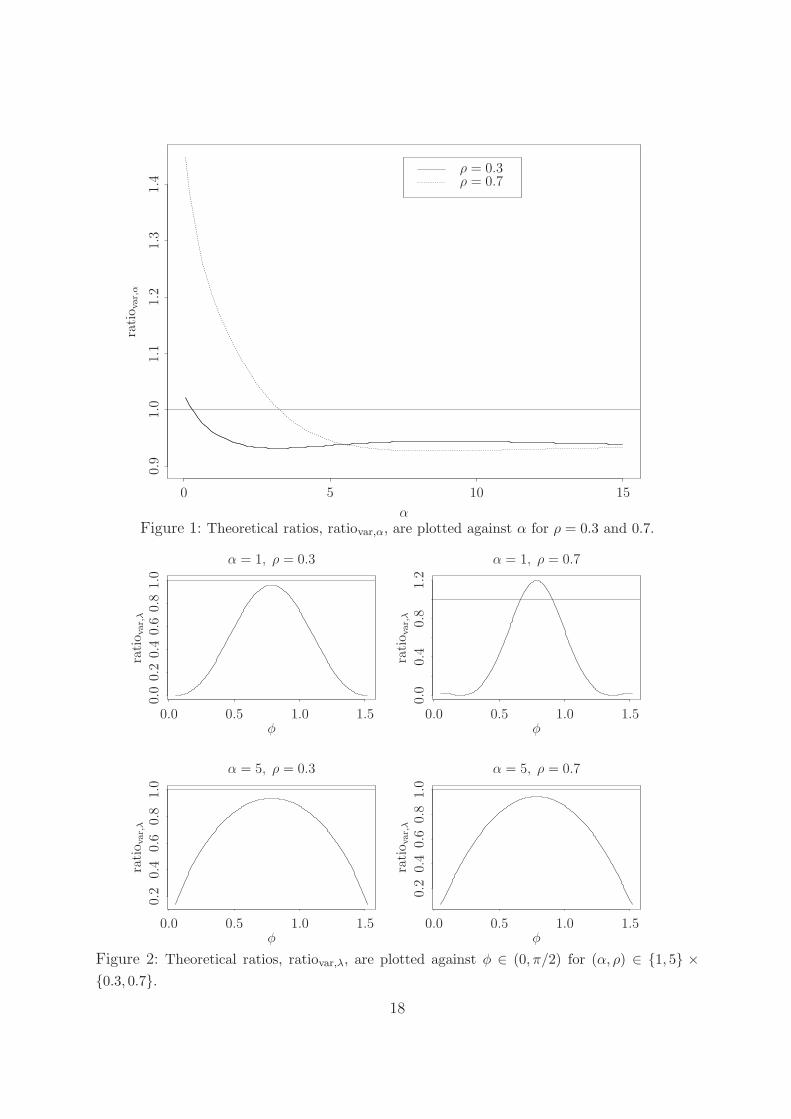
In Figure 1, we plot the ratio ratiovar,α = avarα(w1)/avarα(w0) against α for ρ ∈ {0.3, 0.7},which shows that α(k, w1) has a smaller variance than α(1, 1; k) in many cases, especially

when α is large or ρ is small. Hence α(k, w1) is better than α(1, 1; k) in terms of asymptotic

variance. Without doubt, the weight function w1 is not an optimal one. However, as in

kernel smoothing estimation, we believe that the choice of k is more important than the

choice of w. In practice, we propose to employ the kernel given in (3.1).

Secondly, we compare λ(x, y; k, w) with λemp(x, y; k). It follows from Theorem 2.4 that

the asymptotic variance and the asymptotic mean squared error of λ(x, y; k, w) are

(λ′(α; x, y, ρ))2avarα(k, w) and (λ′(α; x, y, ρ))

2amseα(k, w),

respectively. As in Corollary 3.1, we obtain the optimal asymptotic mean squared error

of λ(x, y; k, w) as (λ′(α; x, y, ρ))2 amseα(k0(w), w). Put

kemp =

(E(B2(x, y))

2βc2(b(C2)(x, y))2

)1/(2β+1)

n2β/(2β+1) and

amseemp(k) = c2(k/n)2β(b(C2)(x, y))2 + k−1E(B2(x, y)).

Then the asymptotic variance and the optimal asymptotic mean squared error of λemp(x, y; k)

are

avarλemp(k, w) = k−1(EB(x, y))2 and amseλemp(k, w) = amseemp(kemp) .

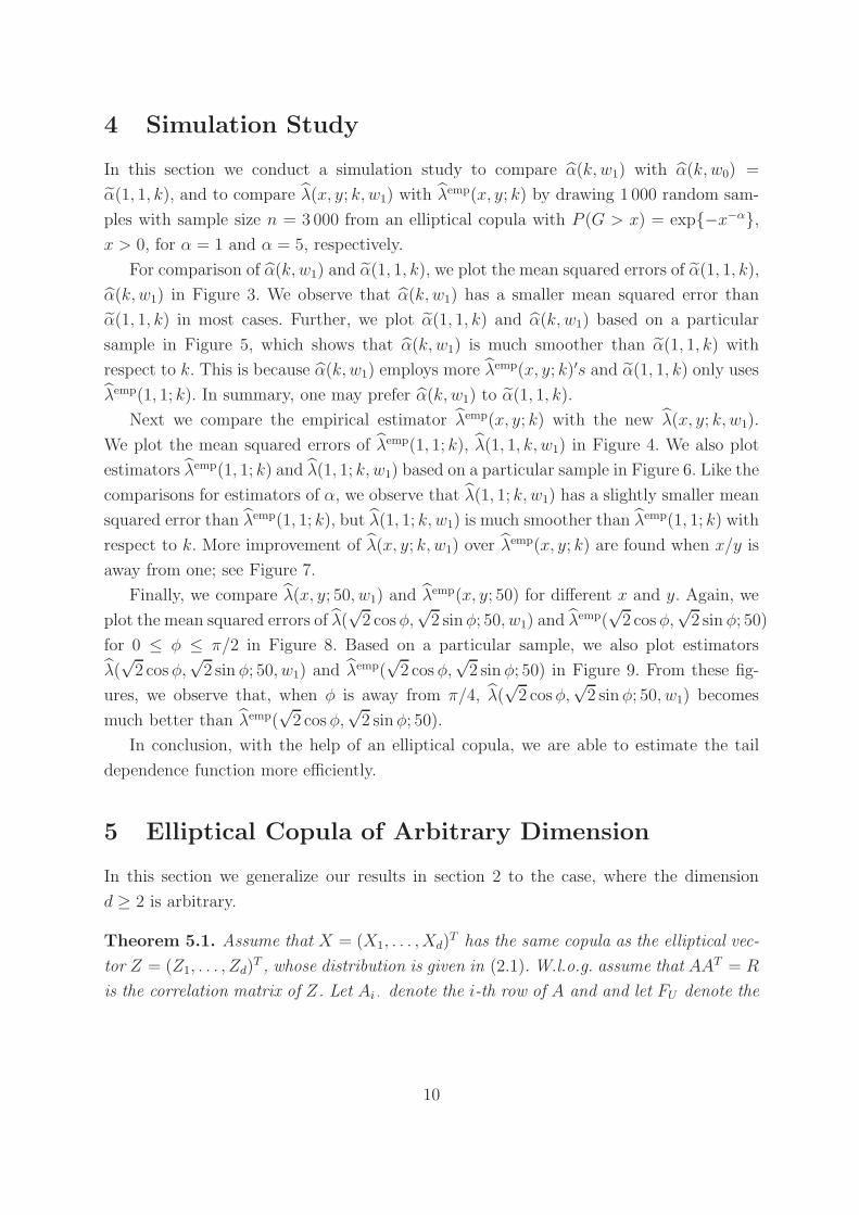
In Figure 2, we plot the ratio of the variances of λ(x, y;w1) and λemp(x, y; k) given by

ratiovar,λ =E(B2(x, y))

(λ′(α; x, y, ρ))2 avarα(w1),

for (x, y) = (√

2 cos φ,√

2 sinφ) against φ ∈ (0, π/2) for different pairs (α, ρ) ∈ {1, 5} ×{0.3, 0.7}, which shows that the new estimator for λX(x, y) has a smaller variance than

the empirical estimator λemp(x, y; k).

9

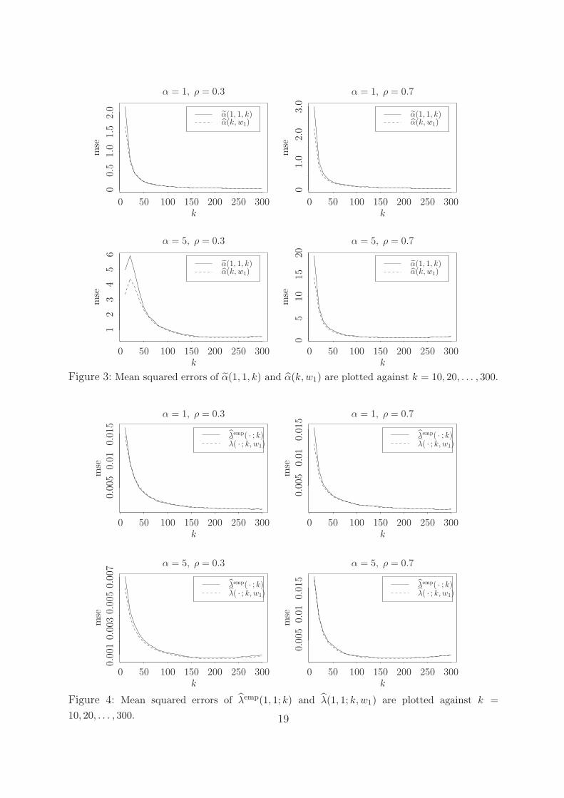
4 Simulation Study

In this section we conduct a simulation study to compare α(k, w1) with α(k, w0) =

α(1, 1, k), and to compare λ(x, y; k, w1) with λemp(x, y; k) by drawing 1 000 random sam-

ples with sample size n = 3 000 from an elliptical copula with P (G > x) = exp{−x−α},x > 0, for α = 1 and α = 5, respectively.

For comparison of α(k, w1) and α(1, 1, k), we plot the mean squared errors of α(1, 1, k),

α(k, w1) in Figure 3. We observe that α(k, w1) has a smaller mean squared error than

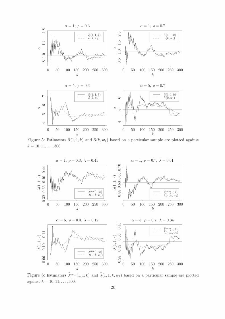
α(1, 1, k) in most cases. Further, we plot α(1, 1, k) and α(k, w1) based on a particular

sample in Figure 5, which shows that α(k, w1) is much smoother than α(1, 1, k) with

respect to k. This is because α(k, w1) employs more λemp(x, y; k)′s and α(1, 1, k) only uses

λemp(1, 1; k). In summary, one may prefer α(k, w1) to α(1, 1, k).

Next we compare the empirical estimator λemp(x, y; k) with the new λ(x, y; k, w1).

We plot the mean squared errors of λemp(1, 1; k), λ(1, 1, k, w1) in Figure 4. We also plot

estimators λemp(1, 1; k) and λ(1, 1; k, w1) based on a particular sample in Figure 6. Like the

comparisons for estimators of α, we observe that λ(1, 1; k, w1) has a slightly smaller mean

squared error than λemp(1, 1; k), but λ(1, 1; k, w1) is much smoother than λemp(1, 1; k) with

respect to k. More improvement of λ(x, y; k, w1) over λemp(x, y; k) are found when x/y is

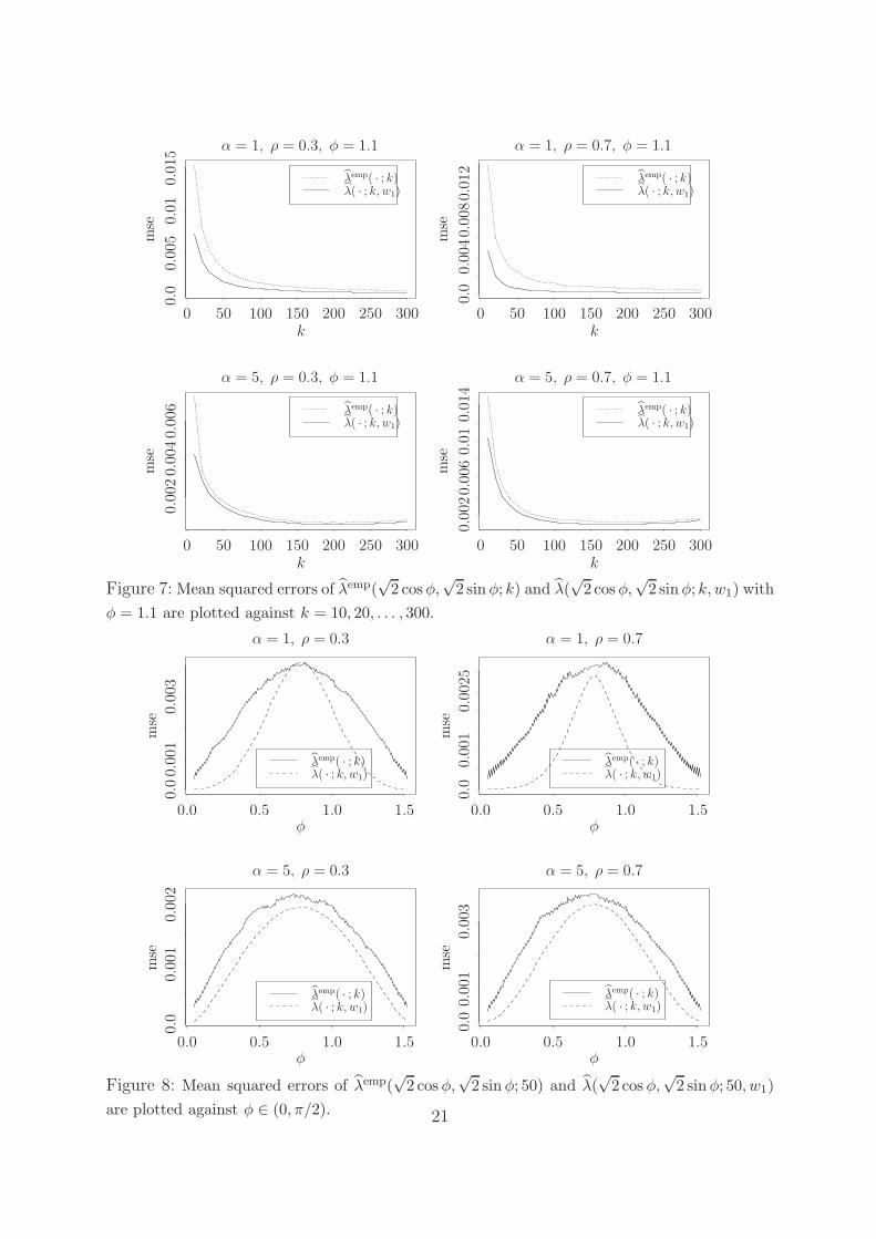
away from one; see Figure 7.

Finally, we compare λ(x, y; 50, w1) and λemp(x, y; 50) for different x and y. Again, we

plot the mean squared errors of λ(√

2 cosφ,√

2 sinφ; 50, w1) and λemp(√

2 cos φ,√

2 sin φ; 50)

for 0 ≤ φ ≤ π/2 in Figure 8. Based on a particular sample, we also plot estimators

λ(√

2 cosφ,√

2 sin φ; 50, w1) and λemp(√

2 cos φ,√

2 sin φ; 50) in Figure 9. From these fig-

ures, we observe that, when φ is away from π/4, λ(√

2 cosφ,√

2 sinφ; 50, w1) becomes

much better than λemp(√

2 cos φ,√

2 sinφ; 50).

In conclusion, with the help of an elliptical copula, we are able to estimate the tail

dependence function more efficiently.

5 Elliptical Copula of Arbitrary Dimension

In this section we generalize our results in section 2 to the case, where the dimension

d ≥ 2 is arbitrary.

Theorem 5.1. Assume that X = (X1, . . . , Xd)T has the same copula as the elliptical vec-

tor Z = (Z1, . . . , Zd)T , whose distribution is given in (2.1). W.l.o.g. assume that AAT = R

is the correlation matrix of Z. Let Ai · denote the i-th row of A and and let FU denote the

10

uniform distribution on Sd. Then the tail dependence function of X is given by

λX(x1, . . . , xd) := limt→0

t−1P (1 − F1(X1) < tx1, . . . , 1 − Fd(Xd) < txd)

=

∫

u∈Sd,A1 · u>0,...,Ad ·u>0

d∧

i=1

xi(Ai ·u)α dFU(u)

( ∫

u∈Sd,A1 · u>0

(A1 ·u)α dFU(u)

)−1

. (5.2)

Remark 5.2. (a) For d = 2 representation (5.2) coincides with (2.2). To see this write u ∈S2 as u = (cos φ, sinφ)T for some φ ∈ (−π, π), A1 · = (1, 0) and A2 · = (ρ,

√1 − ρ2). Then,

Au = (cosφ, ρ cosφ+√

1 − ρ2 sin φ)T = (cosφ, sin(φ+ arcsin ρ))T , giving the equivalence

of (5.2) and (2.2).

(b) For d ≥ 3 one can also use multivariate polar coordinates and obtain analogous

representations. The expression, however, becomes much more complicated.

The estimation procedure in d dimensions is a simple extension of the two-dimensional

case. Assume iid observations Xi = (Xi1, . . . , Xid)T , i = 1, . . . , n, with an elliptical copula.

Then we can estimate ρpq via Kendall’s τ and αpq based on bivariate subvectors (Xip, Xiq)

for 1 ≤ p, q ≤ d. Denote these estimators by ρpq and (for any positive weight function w)

αpq(k, w), respectively. Then we estimate α and R by

α(k, w) =1

d(d− 1)

∑

p 6=q

αpq(k, w) and R = (ρpq)1≤p,q≤d.

Note that R is not necessarily positive semi-definite. In that case we can apply algo-

rithm 3.3 in Higham (2002) to project the indefinite correlation matrix to the class of pos-

itive semi-definite correlation matrices, say AAT = R; see Kluppelberg and Kuhn (2006)

for details. Hence we obtain an estimator for A. This yields an estimator for λ(x1, . . . , xd)

by replacing α and Ai · in (5.2) by α(k, w) and Ai · , respectively. The asymptotic normality

of this new estimator can be derived similarly as in Theorems 2.2 and 2.4.

In Figure 10 we give a three-dimensional example. We simulate a sample of length

n = 3 000 from an elliptical copula with P (G > x) = exp{−x−α}, x > 0, and parameters

ρ12 = 0.3, ρ13 = 0.5, ρ23 = 0.7 and α = 5. In the upper row we plot the true tail de-

pendence function λX(√

3 cosφ1,√

3 sin φ1 cos φ2,√

3 sinφ1 sinφ2

), φ1, φ2 ∈ (0, π/2), and

each column corresponds to perspective, contour and grey-scale image plot of λX , respec-

tively. In the middle and lower row, we plot the corresponding estimators λ(. . . ; 100, w1)

and λemp(. . . ; 100), respectively. From this figure, we also observe that λ becomes much

better than λemp in the three-dimensional case.

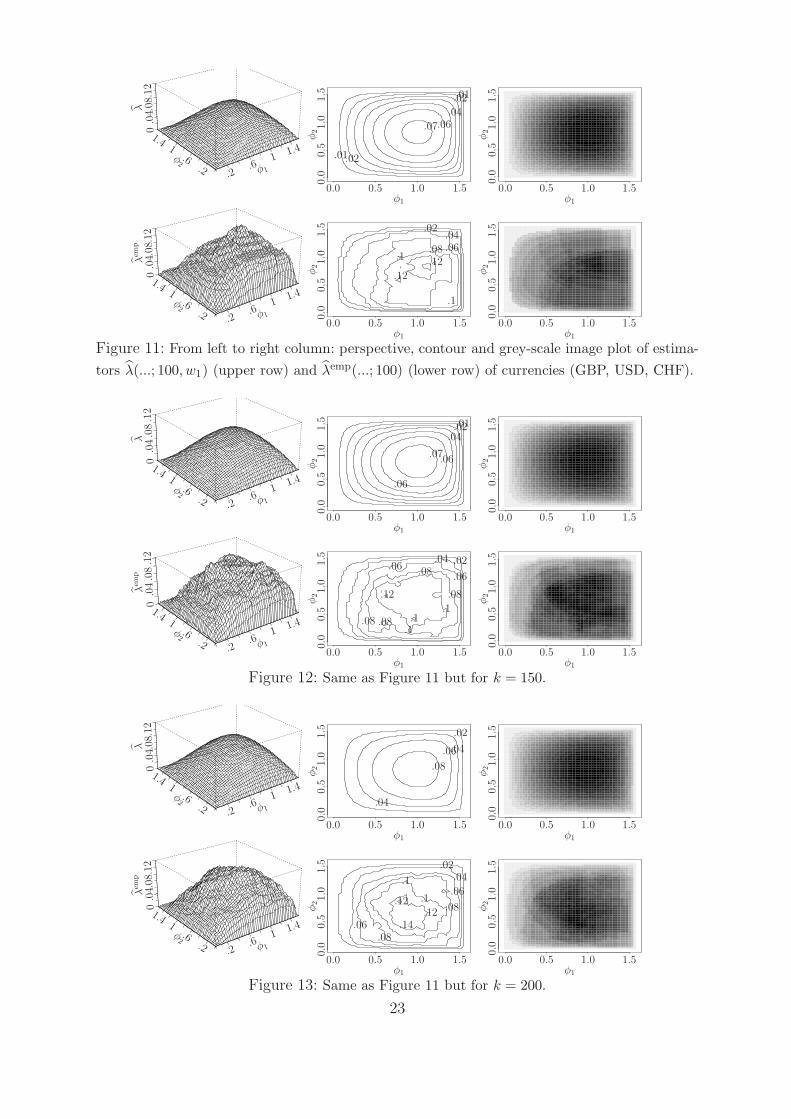
Next we apply our estimators to a three-dimensional real data set which consists of

n = 4 903 daily log returns of currency exchange rates of GBP, USD and CHF with respect

to EURO between May 1985 and June 2004. As in Figure 10, we plot the perspective,

11

contour and grey-scale image of λ(√

3 cosφ1,√

3 sinφ1 cosφ2,√

3 sin φ1 sin φ2; k, w1

)and

λemp(. . . ; k); see Figures 11, 12 and 13 for k = 100, k = 150 and k = 200, respectively.

Comparing the contour plots (middle columns) of λ and λemp, one may conclude that the

assumption of having an elliptical copula is not restrictive.

6 Proofs

We shall use the following notation:

c0 =

∫ π/2

−π/2

(cosφ)α dφ, c1 =

∫ π/2

−π/2

(cosφ)α ln(cos φ) dφ,

D(α, z) = c0

∫ π/2

z

(cosφ)α ln(cosφ) dφ− c1

∫ π/2

z

(cosφ)α dφ and

C(α, z) = D(α, z) +(ρ+

√1 − ρ2 tan z

)−α

D(α, arccos ρ− z).

Recall also from (2.3) that g(t) = arctan((t− ρ)/

√1 − ρ2

)for t > 0.

Lemma 6.1. The tail dependence function λ(α; x, y, ρ) has representation (2.2).

Proof. Kluppelberg, Kuhn and Peng (2007) showed that for an elliptical vector Z

λZ(x, y) =

(∫ π/2

g((x/y)1/α)x(cosφ)α dφ+

∫ g((x/y)1/α)

− arcsin ρ

y (sin(φ+ arcsin ρ))α dφ

)

×(∫ π/2

−π/2

(cosφ)α dφ

)−1

:= λ(α; x, y, ρ).

Since tan(arccos ρ) =(tan(arcsin ρ)

)−1=√

1 − ρ2/ρ, we have

tan(

arccos ρ− g(t))

=tan(arccos ρ) − tan(g(t))

1 + tan(arccos ρ) tan(g(t))=

t−1 − ρ√1 − ρ2

, t > 0,

which implies that

arccos ρ− g(t) = g(t−1), t > 0. (6.1)

Application of a variable transformation to the second summand of (2.2) (setting ψ =

arccos ρ− φ), we obtain (2.2).

Proof of Theorem 2.1. We calculate

cos(g(t)) =(1 +

(t− ρ)2

1 − ρ2

)−1/2

=

√1 − ρ2

√1 − 2tρ+ t2

= t−1 cos(g(t−1)), t > 0. (6.2)

12

It follows from (6.1) and (6.2)

x(cos(g((x/y)1/α))

)α ∂

∂αg((x/y)1/α)+y

(cos(g((x/y)−1/α))

)α ∂

∂αg((x/y)−1/α) = 0. (6.3)

It follows from (6.1) and (6.3) that

la′(α; x, y, ρ) :=∂

∂αλ(α; x, y, ρ)

= c−20

[xD(α, g

((x/y)1/α

))+ yD

(α, g

((x/y)−1/α

))]

= c−20 xC

(α, g

((x/y)1/α

)).

Since

D0,1(α, z) :=∂

∂zD(α, z) = (cos z)α (c1 − c0 ln(cos z)) ,

d2

dz2

(c1 − c0 ln(cos z)

)= c0

(cos z

)−2> 0

and c1 − c0 ln(cos z) is a symmetric function around zero for z ∈ (−π/2, π/2), there exists

0 < z0 < π/2 such that

c1 − c0 ln(cos z) > 0, if z ∈ (−π/2,−z0),c1 − c0 ln(cos z) = 0, if z = −z0,c1 − c0 ln(cos z) < 0, if z ∈ (−z0, z0),c1 − c0 ln(cos z) = 0, if z = z0,

c1 − c0 ln(cos z) > 0, if z ∈ (z0, π/2)

i.e.,

D0,1(α, z) > 0, if z ∈ (−π/2,−z0),D0,1(α, z) = 0, if z = −z0,D0,1(α, z) < 0, if z ∈ (−z0, z0),D0,1(α, z) = 0, if z = z0,

D0,1(α, z) > 0, if z ∈ (z0, π/2).

Note that z0 depends on α. Since D(α, 0) = limz→±π/2

D(α, z) = 0, we have

{D(α, z) > 0, if z ∈ (−π/2, 0),

D(α, z) < 0, if z ∈ (0, π/2).

Hence, if x/y ∈[(ρ ∨ 0)α∗

, (ρ ∨ 0)−α∗]

for some α∗ ∈ (0,∞), then C(α, g

((x/y)1/α∗

))< 0

for all α > α∗. Since also x/y ∈ [(ρ ∨ 0)α, (ρ ∨ 0)−α] holds for all α > α∗, we have

C(α, g

((x/y)1/α

))< 0 for all α > α∗. Hence the theorem follows by choosing α∗ =

|ln(x/y)/ ln(ρ ∨ 0)|.

13

Proof of Theorem 2.2. Using the same arguments as in Lemma 1 of Huang (1992),

p. 30, or Corollary 3.8 of Einmahl (1997), we can show that

sup0<x,y<T

∣∣∣√k(λemp(x, y) − λX(x, y)

)− b(C3)b(C2)(x, y) − B(x, y)

∣∣∣ = op(1) (6.4)

as n → ∞. Note that the above equation can also be shown in a way similar to Schmidt

and Stadtmuller (2005) by taking the bias term into account. Since λ(α; x, y, ρ) in (2.2) is

a continuous function of α, by invoking the delta method, the theorem follows from (6.4),

τ − τ = op(1/√k) (see Kluppelberg and Kuhn (2006), Theorem 4.6),

supθ∈Q∗

|λ′(α;√

2 cos θ,√

2 sin θ, ρ)| <∞,

and a Taylor expansion.

Proof of Theorem 2.4. It easily follows from (2.2) and Theorem 2.2.

Proof of Theorem 5.1. Since copulas are invariant under strictly increasing transfor-

mations, we can assume w.l.o.g that AAT = R is the correlation matrix. Therefore, the

Zid= GAi ·U , 1 ≤ i ≤ d, have the same distribution, say FZ . Hence

P (1 − FZ(Z1) < tx1, . . . , 1 − FZ(Zd) < txd)

=

∫

u∈Sd,A1 · u>0,...,Ad ·u>0

P(G >

d∨

i=1

F←Z (1 − txi)

Ai ·u

)dFU(u), (6.5)

where F←Z denotes the inverse function of FZ . Since P (G > · ) ∈ RV−α implies that

1 − FZ ∈ RV−α, the inverse function F←Z ∈ RV−1/α (e.g. Resnick (1987), Proposition

0.8(v)). This implies

limt→0

P (G > F←Z (1 − txi)/(Ai ·u))

P (G > F←Z (1 − t))= xi(Ai ·u)

α, i = 1, . . . , d.

Now note that, for all i = 1, . . . , d,

t = P (Zi > F←Z (1 − t)) = P (GAi ·U > F←Z (1 − t))

=

∫

u∈Sd,Ai · u>0

P

(G >

F←Z (1 − t)

Ai ·u

)dFU(u),

giving by means of Potter’s bounds (e.g. see (1.20) in Geluk and de Haan (1987)),

limt→0

t

P (G > F←Z (1 − t))= lim

t→0

∫

u∈Sd,Ai · u>0

P (G > F←Z (1 − t)/(Ai ·u))

P (G > F←Z (1 − t))dFU(u)

=

∫

u∈Sd,Ai · u>0

(Ai ·u)α dFU(u) ∀i = 1, . . . , d. (6.6)

14

Applying the same method to (6.5) yields the proof.

Acknowledgment. Peng’s research was supported by NSF grants DMS-0403443 and

SES-0631608, and a Humboldt Research Fellowship.

References

Abdous, B., Fougeres, A.-L. and Ghoudi, K. (2005). Extreme behaviour for bivariate

elliptical distributions. Canadian J. Statist. 33, 317-334.

Abdous, B., Ghoudi, K. and Khoudraji, A. (1999). Non-parametric estimation of the limit

dependence function of multivariate extremes. Extremes 2(3), 245-268.

Coles, S.G. (2001). An Introduction to Statistical Modeling of Extreme Values. Springer,

London.

Draisma, G., Drees, H., Ferreira, A. and de Haan, L. (2004). Bivariate tail estimation:

dependence in asymptotic independence. Bernoulli 10, 251-280.

Einmahl, J.H.J. (1997). Poisson and Gaussian approximation of weighted local empirical

processes. Stoch. Proc. Appl. 70, 31-58.

Einmahl, J.H.J., de Haan, L. and Li, D. (2006). Weighted approximations of tail copula

processes with applications to testing the multivariate extreme value condition. Ann.

Statist. 34, 1987-2014.

Einmahl, J.H.J., Haan, L. de and Piterbarg, V.I. (2001). Nonparametric estimation of the

spectral measure of an extreme value distribution. Ann. Statist. 29, 1401 - 1423.

Falk, M. and Reiss, R.-D. (2005). On Pickands coordinates in arbitrary dimension. J.

Multivariate Anal. 92, 426-453.

Fang, K.-T., Kotz, S. and Ng, K.-W. (1987). Symmetric Multivariate and Related Distri-

butions. Chapman & Hall, London.

Galambos, J.(1987). The Asymptotic Theory of Extreme Order Statistics. 2nd Ed. Krieger

Publishing Co., Malabar, Florida.

Gumbel, E.J. (1960). Bivariate exponential distributions. J. Am. Statist. Assoc. 55, 698-

707.

Geluk, J. and de Haan, L. (1987). Regular Variation, Extensions and Tauberian Theorems.

15

CWI Tract 40.

Heffernan, J.E. and Tawn, J.A. (2004). A conditional approach to modelling multivariate

extreme values (with discussion). J. Roy. Statist. Soc., Ser. B 66, 497 - 547.

Higham, N. (2002). Computing the nearest correlation matrix - a problem from finance.

IMA J. Numer. Anal. 22(3), 329-343.

Hoeffding, W. (1948). A class of statistics with asymptotically normal distribution. Ann.

Math. Statist. 19, 293-325.

Hsing, T., Kluppelberg, C. and Kuhn, G. (2004). Dependence estimation and visualization

in multivariate extremes with application to financial data. Extremes 7(2), 99-121.

Huang, X. (1992). Statistics of Bivariate Extreme Values. Ph.D. Thesis, Tinbergen Insti-

tute Research Series.

Hult, H. and Lindskog, F. (2002). Multivariate extremes, aggregation and dependence in

elliptical distributions. Adv. Appl. Prob. 34(3), 587 - 608.

Joe, H. (1997). Multivariate Models and Dependence Concepts. Chapman & Hall, London.

Juri, A. and Wuthrich, M.V. (2002). Copula convergence theorems for tail events. Insur-

ance: Math. & Econom. 30, 411-427.

Kallsen, J. and Tankov, P. (2006). Characterization of dependence of multidimensional

Levy processes using Levy copulas. J. Multiv. Anal. 97, 1551-1572.

Kluppelberg, C. and Kuhn, G. (2006) Copula structure analysis. Submitted for publica-

tion. Available at www.ma.tum.de/stat/

Kluppelberg, C., Kuhn, G. and Peng, L. (2007). Estimating the tail dependence of an

elliptical distribution. Bernoulli 13(1), 229 - 251.

Ledford, A.W. and Tawn, J.A. (1997). Modelling dependence within joint tail regions. J.

Roy. Statist. Soc. Ser. B 59, 475 - 499.

Lee, A. (1990) U-Statistics. Marcel Dekker, New York.

McNeil, A., Frey, R. and Embrechts, P. (2005) Quantitative Risk Management. Princeton

University Press, Princeton.

16

Nelsen, R.B. (1998). An Introduction to Copulas. Lecture Notes in Statistics 139, Springer,

New York.

Peng, L. and Qi, Y. (2007). Partial derivatives and confidence intervals of bivariate tail

dependence functions. Journal of Statistical Planning and Inference 137, 2089 - 2101.

Pickands, J. (1981). Multivariate extreme value distributions. Bull. Int. Statisti. Inst.,

859-878.

Resnick, S.I. (1987). Extreme Values, Regular Variation and Point Processes. Springer,

New York.

Schmidt, R. and Stadtmuller, U. (2006). Nonparametric estimation of tail dependence.

Scand. J. Stat. 33(2), 307-335.

Tawn, J.A. (1988). Bivariate extreme value theory: models and estimation. Biometrika

75, 397 - 415.

17

α

rati

o var,

α

ρ = 0.3ρ = 0.7

0.9

1.0

1.1

1.2

1.3

1.4

0 5 10 15

Figure 1: Theoretical ratios, ratiovar,α, are plotted against α for ρ = 0.3 and 0.7.1

rati

o var,

λ

rati

o var,

λ

rati

o var,

λ

rati

o var,

λ

φφ

φφ

0.00.0

0.0

0.0

0.0

0.0

0.50.5

0.50.5

1.0

1.0

1.0

1.0

1.0

1.0

1.0

1.51.5

1.51.5

0.2

0.2

0.2

0.4

0.4

0.40.4

0.6

0.6

0.6

0.8

0.8

0.80.

8

1.2

α = 1, ρ = 0.3 α = 1, ρ = 0.7

α = 5, ρ = 0.3 α = 5, ρ = 0.7

Figure 2: Theoretical ratios, ratiovar,λ, are plotted against φ ∈ (0, π/2) for (α, ρ) ∈ {1, 5} ×{0.3, 0.7}.

18

mse

mse

mse

mse

kk

kk

α = 1, ρ = 0.3 α = 1, ρ = 0.7

α = 5, ρ = 0.3 α = 5, ρ = 0.7

α(1, 1, k)α(1, 1, k)

α(1, 1, k)α(1, 1, k)

α(k, w1)α(k, w1)

α(k, w1)α(k, w1)

0

00

00

5050

5050

100100

100100

150150

150150

200200

200200

250250

250250

300300

300300

000.

5 1.01.

01.

5

2.0

2.0 3.0

12

34

5

56

1015

20

Figure 3: Mean squared errors of α(1, 1, k) and α(k,w1) are plotted against k = 10, 20, . . . , 300.

mse

mse

mse

mse

kk

kk

α = 1, ρ = 0.3 α = 1, ρ = 0.7

α = 5, ρ = 0.3 α = 5, ρ = 0.7

λemp( · ; k)λemp( · ; k)

λemp( · ; k)λemp( · ; k)

λ( · ; k, w1)λ( · ; k, w1)

λ( · ; k, w1)λ( · ; k, w1)

00

00

5050

5050

100100

100100

150150

150150

200200

200200

250250

250250

300300

300300

0.00

5

0.00

5

0.00

5

0.00

5

0.01

0.01

0.01

0.01

50.

015

0.01

50.

001

0.00

30.

007

Figure 4: Mean squared errors of λemp(1, 1; k) and λ(1, 1; k,w1) are plotted against k =

10, 20, . . . , 300. 19

αα

αα

kk

kk

α = 1, ρ = 0.3 α = 1, ρ = 0.7

α = 5, ρ = 0.3 α = 5, ρ = 0.7

α(1, 1, k)α(1, 1, k)

α(1, 1, k)α(1, 1, k)

α(k, w1)α(k, w1)

α(k, w1)α(k, w1)

00

00

5050

5050

100100

100100

150150

150150

200200

200200

250250

250250

300300

300300

.8

1.0

1.0

1.4

1.8

0.5

1.5

2.0

45

67

45

6

Figure 5: Estimators α(1, 1, k) and α(k,w1) based on a particular sample are plotted against

k = 10, 11, . . . , 300.

λ(1,1

;·)

λ(1,1

;·)

λ(1,1

;·)

λ(1,1

;·)

kk

kk

α = 1, ρ = 0.3, λ = 0.41 α = 1, ρ = 0.7, λ = 0.61

α = 5, ρ = 0.3, λ = 0.12 α = 5, ρ = 0.7, λ = 0.34

λemp( · ; k)

λemp( · ; k)

λemp( · ; k)λemp( · ; k)

λ( · ; k, w1)

λ( · ; k, w1)

λ( · ; k, w1)λ( · ; k, w1)

00

00

5050

5050

100100

100100

150150

150150

200200

200200

250250

250250

300300

300300

0.32

0.32

0.36

0.36

0.40

0.40

0.44

0.55

0.60

0.65

0.70

0.06

0.10

0.14

0.28

Figure 6: Estimators λemp(1, 1; k) and λ(1, 1; k,w1) based on a particular sample are plotted

against k = 10, 11, . . . , 300.

20

mse

mse

mse

mse

kk

kk

α = 1, ρ = 0.3, φ = 1.1 α = 1, ρ = 0.7, φ = 1.1

α = 5, ρ = 0.3, φ = 1.1 α = 5, ρ = 0.7, φ = 1.1

λemp( · ; k)λemp( · ; k)

λemp( · ; k)λemp( · ; k)

λ( · ; k, w1)λ( · ; k, w1)

λ( · ; k, w1)λ( · ; k, w1)

00

00

5050

5050

100100

100100

150150

150150

200200

200200

250250

250250

300300

300300

0.0

0.0

0.00

5

0.01

0.01

0.01

50.

004

0.00

40.

0080.

012

0.00

2

0.00

2

0.00

6

0.00

6

0.01

4

Figure 7: Mean squared errors of λemp(√

2 cos φ,√

2 sin φ; k) and λ(√

2 cos φ,√

2 sin φ; k,w1) with

φ = 1.1 are plotted against k = 10, 20, . . . , 300.

.012

mse

mse

mse

mse

φφ

φφ

α = 1, ρ = 0.3 α = 1, ρ = 0.7

α = 5, ρ = 0.3 α = 5, ρ = 0.7

λemp( · ; k)λemp( · ; k)

λemp( · ; k)λemp( · ; k)

λ( · ; k, w1)λ( · ; k, w1)

λ( · ; k, w1)λ( · ; k, w1)

0.0

0.0

0.0

0.0

0.0

0.0

0.0

0.0

0.50.5

0.50.5

1.01.0

1.01.0

1.51.5

1.51.5

0.00

1

0.00

1

0.00

3

0.00

30.

001

0.00

1

0.00

2

0.00

25

Figure 8: Mean squared errors of λemp(√

2 cos φ,√

2 sin φ; 50) and λ(√

2 cos φ,√

2 sin φ; 50, w1)

are plotted against φ ∈ (0, π/2). 21

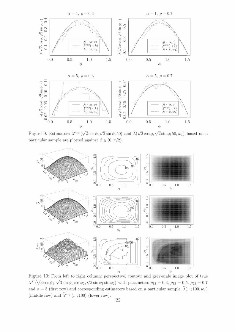
λ(√

2co

sφ,√

2si

nφ;·)

λ(√

2co

sφ,√

2si

nφ;·)

λ(√

2co

sφ,√

2si

nφ;·)

λ(√

2co

sφ,√

2si

nφ;·)

φφ

φφ

α = 1, ρ = 0.3 α = 1, ρ = 0.7

α = 5, ρ = 0.3 α = 5, ρ = 0.7

λ( · ;α, ρ)λ( · ;α, ρ)

λ( · ;α, ρ)λ( · ;α, ρ)

λemp( · ; k)λemp( · ; k)

λemp( · ; k)λemp( · ; k)

λ( · ; k, w1)λ( · ; k, w1)

λ( · ; k, w1)λ( · ; k, w1)

0.00.0

0.00.0

0.50.50.

5

0.50.5

1.01.0

1.01.0

1.51.5

1.51.5

0.10.

10.

2

0.3

0.3

0.4

0.05

0.15

0.25

0.35

0.02

0.06

0.10

0.14

Figure 9: Estimators λemp(√

2 cos φ,√

2 sin φ; 50) and λ(√

2 cos φ,√

2 sin φ; 50, w1) based on a

particular sample are plotted against φ ∈ (0, π/2).

λX

λλ

emp

φ1φ1

φ1

φ1φ1

φ1

φ1φ1

φ1

φ2

φ2

φ2

φ2

φ2

φ2

φ2

φ2

φ2

0.0

0.0

0.0

0.0

0.0

0.0

0.0

0.0

0.0

0.0

0.0

0.0

0.5

0.5

0.5

0.5

0.5

0.5

0.5

0.5

0.5

0.5

0.5

0.5

1.0

1.0

1.0

1.0

1.0

1.0

1.0

1.0

1.0

1.0

1.0

1.0

1.5

1.5

1.5

1.5

1.5

1.5

1.5

1.5

1.5

1.5

1.5

1.5

.2 .2

.2 .2

.2 .2

.6.6

.6.6

.6.6

11

11

11

1.41.4

1.41.4

1.41.4

.02

.02

.02

.02

.02

.02

.06.06

.06

.06

.06

.06

.06

.08

.08

.1

.1.1

.1

.07

Figure 10: From left to right column: perspective, contour and grey-scale image plot of true

λX(√

3 cos φ1,√

3 sin φ1 cos φ2,√

3 sinφ1 sin φ2

)with parameters ρ12 = 0.3, ρ13 = 0.5, ρ23 = 0.7

and α = 5 (first row) and corresponding estimators based on a particular sample, λ(...; 100, w1)

(middle row) and λemp(...; 100) (lower row).22

λλ

emp

φ1φ1

φ1

φ1φ1

φ1

φ2

φ2

φ2

φ2

φ2

φ2

0.0

0.00.

00.0

0.0

0.0

0.0

0.0

0.5

0.50.

50.5

0.5

0.5

0.5

0.5

1.0

1.01.

01.0

1.0

1.0

1.0

1.0

1.5

1.51.

51.5

1.5

1.5

1.5

1.5

.2 .2

.2 .2

.6.6

.6.6

11

11

1.41.4

1.41.4 .01

.01

.02

.02

.02

.04

.04

.06

.06

.08

.1

.1 .12

.1200

.04

.04

.08

.08

.12

.12

.07

Figure 11: From left to right column: perspective, contour and grey-scale image plot of estima-

tors λ(...; 100, w1) (upper row) and λemp(...; 100) (lower row) of currencies (GBP, USD, CHF).

λλ

emp

φ1φ1

φ1

φ1φ1

φ1

φ2

φ2

φ2

φ2

φ2

φ2

0.0

0.0

0.0

0.0

0.0

0.0

0.0

0.0

0.5

0.5

0.5

0.5

0.5

0.5

0.5

0.5

1.0

1.0

1.0

1.0

1.0

1.0

1.0

1.0

1.5

1.5

1.5

1.5

1.5

1.5

1.5

1.5

.2 .2

.2 .2

.6.6

.6.6

11

11

1.41.4

1.41.4

.01

.02

.02

.04

.04

.06.06

.06

.06

.08

.08

.08.08 .1.1

.1

.12

00

.04

.04

.08

.08

.12

.12

.07

Figure 12: Same as Figure 11 but for k = 150.

λλ

emp

φ1φ1

φ1

φ1φ1

φ1

φ2

φ2

φ2

φ2

φ2

φ2

0.0

0.0

0.0

0.0

0.0

0.0

0.0

0.0

0.5

0.5

0.5

0.5

0.5

0.5

0.5

0.5

1.0

1.0

1.0

1.0

1.0

1.0

1.0

1.0

1.5

1.5

1.5

1.5

1.5

1.5

1.5

1.5

.2 .2

.2 .2

.6.6

.6.6

11

11

1.41.4

1.41.4

.02

.02

.04

.04

.04

.06

.06

.06

.08

.08

.08

.1

.1

.12.12

.14

00

.04

.04

.08

.08

.12

.12

Figure 13: Same as Figure 11 but for k = 200.

23