selection of copulas with applications in...

Selection of Copulas with Applications in Finance∗

Zongwu Caia,b, Xiaohong Chenc, Yanqin Fand, and Xian Wanga

aDepartment of Mathematics & Statistics, University of North Carolina at Charlotte,

Charlotte, NC 28223, USA, E-mails: [email protected] (Z. Cai) and [email protected] (X. Wang)bThe Wang Yanan Institute for Studies in Economics, Xiamen University, China

cDepartment of Economics, Yale University, New Haven, CT 06520, USA, E-mail: [email protected] of Economics, Vanderbilt University, Nashville, TN 37240, USA, E-mail: [email protected]

First Draft: March 5, 2008

A fundamental issue of applying copula method in applications is how to choose an appro-priate copula function. In this article we address this issue by proposing a new copula selectionapproach via penalized likelihood. The proposed method selects the appropriate copula func-tions and estimates copula coefficients simultaneously. The asymptotic properties, including therate of convergence and asymptotic normality and abnormality, are established for the proposedpenalized likelihood estimator. Particularly, when the true coefficient parameters may be onthe boundary of the parameter space and the dependence parameters are in an unidentifiablesubset of the parameter space, it shows that the limiting distribution for boundary parametersis abnormal and the penalized likelihood estimator for unidentified parameters converges to anarbitrary value. Moreover, the EM algorithm is proposed for optimizing penalized likelihoodfunction. Finally, Monte Carlo simulation studies are carried out to illustrate the finite sam-ple performance of the proposed method and the proposed method is used to investigate thecorrelation structure and comovement of financial stock markets.

Keywords: EM algorithm; Mixed copula; Penalized likelihood; SCAD; Variable selection.

∗The authors thank Yoon-Jae Whang and other audiences at Sino-Korean Workshop 2007 in Xiamen for theirconstructive comments and suggestions.

1 Introduction

Copula approach has been used in many financial and economic fields recently, such as, asset pric-

ing, risk management, portfolio and market value-at-risk calculations, and correlation structure and

movement of the financial market. For example, Li (2000) was the first to study the default correla-

tions in credit risk models by using the copula function to model the joint distribution between two

default times. Bouye, Nikeghbali, Riboulet and Roncalli (2001), Embrechts, Lindskog and McNell

(2003), and Cherubini, Vecchiato and Luciano (2004) applied the copula functions to measure the

portfolio value-at-risk. Longin and Solnik (2001) examined cross-national dependence structure

of asset returns in international financial market. Ang and Chen (2002) discovered asymmetric

dependence between two asset returns during market downturns and market upturns. Although

copula method has been applied to financial fields recently, it grows swiftly due to its several ad-

vantages. First, copulas are invariant to strictly increasing transformations of random variables.

This property is very useful as transformations, such as log-transformation, are commonly used in

financial analysis. Secondly, nonparametric dependence measures, like Kendall’s τ and Spearman’s

ρ, are properties of copula functions. It is well known that economic and financial multivariate time

series are typically nonlinear, abnormally distributed, and have nonlinear comovement. By using

nonparametric measures, the assumptions like Gaussian distribution or linear dependence required

for the correlation coefficient can be relaxed. Thirdly, asymptotic tail dependence measures de-

pendence between extreme values. This property implies that copula functions enable us to model

different patterns of dependence structures. Finally, by Sklar’s (1959) theorem, any multidimen-

sional joint distribution function may be decomposed into its marginal distributions and a copula

function which completely describes the dependence structure. Indeed, copulas allow us to model

fat tails of the marginal distributions and tail dependence separately.

As aforementioned, copulas can be used to model the different patterns of dependence structures.

For example, a Gaussian copula model has zero tail dependence, which means the probability that

both variables are in their extremes is asymptotically zero unless their linear correlation coefficient

1

is unit. A Gumbel copula has a positive right tail dependence, i.e., the probability that both

variables are in the right tails is positive. To capture different shapes of distributions and different

patterns of dependence structure, researchers have considered a mixed copula which is a linear

combination of several copula families. For example, Hu (2003) used a mixed copula approach

with predetermined coefficients to measure the dependence patten across financial markets. The

mixture copula used in Hu (2003) is composed of a Gaussian copula, a Gumbel copula and a

Gumbel survival copula. Clearly, a Gaussian copula is chosen based on the traditional approach

and the other two copulas are selected to take into account of possible left and right tail dependence.

Chollete, Pena, and Lu (2005) analyzed the co-movement of international financial markets by using

a mixed copula model. They considered the same mixture as Hu (2003) and another mixture by

replacing Gaussian copula with t-copula. The biggest advantage of using a mixed copula model

is that it can nest different copula shapes, i.e., mixed copulas can capture different patterns of

dependence structure. For example, if we consider a mixed copula which includes Gaussian and

Gumbel copulas, it can improve a single Gaussian dependence structure by allowing possible right

tail dependence. Therefore, empirically, a mixed copula is more flexible to model the dependence

and can deliver better descriptions of dependence structure than an individual copula.

For applying the copula approach to solve real problems, it is important to choose appropriate

parametric or nonparametric copulas since the distribution from which each data point is drawn

is unknown. To attenuate this problem, there have been some efforts in literature to choose an

appropriate individual copula, while Chen, Fan and Patton (2003) and Fermanian (2003) developed

goodness-of-fit tests of an individual parametric copula. But there is no guidance as to which

copula model should be used if these tests are used and the null hypothesis of correct parametric

specification is rejected. Further, Hu (2003) considered a mixed copula by deleting the component

if the corresponding weight is less than 0.1 or if the corresponding dependence measure is close

to independence. To the best of our knowledge, so far no work with theoretical support has been

attempted to choose the suitable copulas for a mixed copula.

2

In this paper, we propose a copula selection method via penalized likelihood. Initially, a large

number of candidate copula families are of interest and their contributions to the dependence

structure vary from one component to another. Our task is to select an appropriate copula or several

copulas which can capture the dependence structure of the given data set among the candidate

copulas. As we stated earlier, copula function can be used to describe the joint distribution.

Therefore, this question can be solved by searching a copula or the mixture of several copulas that

produce the highest likelihood. To select and estimate a mixed copula simultaneously, we formulate

the problem of copula selection as the problem of variable selection. When the fitted mixed copula

contains some component copulas which have small weight (small contribution to the dependence

structure), we expect these components would not be in the mixed copula. This idea is in principle

similar to the approach in Fan and Li (2001) and Fan and Peng (2004) based on a penalty function

to delete the insignificant variables and to estimate the coefficients of significant variables in the

context of regression settings. Chen and Khalili (2006) applied the variable selection method to

the order selection in finite mixture models. In contrast, our approach can be formulated as the

penalized likelihood function with an appropriate penalty function. By maximizing the penalized

likelihood function, copulas with small weights are removed by a thresholding rule and parameters

remained are estimated. In such a way, the model selection and parameter estimation can be

done simultaneously. We show that this method is less computing intensive than many other

existing methods which select an appropriate copula. Also the new method has a high probability

of selecting an appropriate mixed copula model. Further, we establish the asymptotic properties

of the proposed estimators. It is interesting to note that the general mathematical derivation for

the asymptotic properties for the maximum likelihood estimator is not applicable here since the

parameters may not be an interior point of the parameter space, which was addressed by Andrew

(1999) for the case when the parameter is on a boundary for iid sample. Therefore, the challenges

we face here are not only that the coefficient parameters are on the boundary of the parameter

space but also that the dependent parameters are in a non-identifiable subset of the parameter

3

space. Thus, another two main contributions are, under this non-standard situation, we show

that the estimate of non-identifiable dependent parameters converge to arbitrary value and we

establish the abnormality of the boundary coefficient parameter estimate. Finally, to make the

proposed methodology practically useful and applicable, we propose using the EM algorithm to

find the penalized likelihood estimators. Also, we consider the data-driven methods for finding

the threshold parameters in the penalty function. Further, we suggest an ad hoc method for a

consistent estimator of the standard error.

The rest of this paper is organized as follows. Section 2 briefly reviews some basic facts about

copulas and discusses the identification of the mixed copula model. In Section 3, we introduce the

selection procedure based on the penalized likelihood. In Section 4, we list the regularity conditions

and develop the asymptotic properties of the proposed estimators. The EM algorithm is outlined for

finding the penalized likelihood estimators and the data-driven methods for finding the threshold

parameters are discussed in Section 5, together with an ad hoc method for proposing a consistent

estimator of the standard error. In Section 6, the results of a Monte Carlo study are reported

to demonstrate the finite sample performance of the proposed methods, together with empirical

analyses of real financial data. The technical proofs are collected in Section 7.

2 Mixed Copulas

2.1 Copulas

For simplicity of presentation, we only consider the two-dimensional case. Indeed, all methods and

theory developed here continue to hold for multivariate case. The only difference for multivariate

is the computing issue. We consider an i.i.d sequence {(Xt, Yt), t ∈ Z} taking values in R2 with a

realization of {(Xt, Yt); 1 ≤ t ≤ T}. We denote by f(x, y), F (x, y), the joint density and distribution

of {(Xt, Yt)}. The joint distribution F (·, ·) completely determine the probabilistic properties of

{(Xt, Yt)}. F (·, ·) can be expressed as a copula function between Xt and Yt and marginal distribution

functions of Xt and Yt. Let fx(x) and fy(y) be the marginal density of Xt and Yt. The marginal

distribution of Xt and Yt are written as Fx(x) and Fy(y), respectively. Now we would like to review

4

some formal copula and useful dependence concepts. For more discussions, the reader is referred

to the books by Nelsen (1999) and Joe (1997).

Definition 1: A two-dimensional copula is a function C(·, ·): [0, 1]2 → [0, 1] with the following

properties:

1. C is grounded, i.e., for every (u, v) in [0, 1]2, C(u, v) = 0 if at least one coordinate is 0.

2. C is two-increasing, i.e., for every a and b in [0, 1]2 such that a ≤ b, the C-volume VC([a, b]) of

the box [a, b] is positive.

3. C(u, 1) = u and C(1, v) = v for every (u, v) ∈ [0, 1]2.

One can think of a copula as a function which assigns any point in the unit square [0, 1] ×

[0, 1] a number in the interval [0, 1]. From a probabilistic point of view, a copula function is

a joint distribution whose marginal distributions are uniform. Next, we would like to state the

famous Sklar’s (1959) theorem which links the univariate margins and the multivariate dependence

structure.

Sklar’s Theorem: (Sklar (1959)). Let F (x, y) be a bivariate distribution function with margins

Fx(x) and Fy(y). Then, there exists a bivariate copula C such that for all (x, y) in R2,

F (x, y) = C(Fx(x), Fy(y)). (1)

If Fx(x) and Fy(y) are all continuous, then C is uniquely defined. Otherwise, C is uniquely

determined on RangeFx(x) × RangeFy(y). Conversely, if C is a bivariate copula and Fx(x) and

Fy(y) are distribution functions, then the function F (x, y) defined by (1) is a bivariate distribution

function with margins Fx(x) and Fy(y).

As an immediate result of Sklar’s theorem, F (x, y) can be expressed in terms of the marginal

distribution functions of Xt and Yt and the copula function of Xt and Yt. That is,

F (x, y) = C(Fx(x), Fy(y)).

5

More specifically, if we consider a parametric model in which the marginal distributions Fx(x) and

Fy(y) depend on the distinct parameters α and β, we have

F (x, y; α, β, θ) = C(Fx(x; α), Fy(y; β); θ), (2)

where θ is the dependence parameter in copula. To avoid confusion, we need to note that x and

y are used to denote the actual observations, such as the returns in different markets. And we

use u and v to denote the marginal distribution of x and y. So x and y are any real numbers but

u, v ∈ [0, 1].

Another useful concept in copula field is tail dependence. It measures the dependence between

two variables in the upper and lower joint tail values of two variables.

Definition 2: Let X and Y be continuous random variables with copula C and marginal distri-

bution functions Fx(x) and Fy(y). The coefficients of upper and lower tail dependence of (Xt, Yt)

are defined as

τU = limv→1

Pr(Fy(y) > v|Fx(x) > v) = limv→1

1 − 2v + C(v, v)

1 − v

and

τL = limv→0

Pr(Fy(y) ≤ v|Fx(x) ≤ v) = limv→0

C(v, v)

v

provided that the limit τU ∈ [0, 1] and τL ∈ [0, 1] exist.

Tail dependence is a copula property and the amount of tail dependence is invariant under

strictly increasing transformations of X and Y . If τU ∈ (0, 1], X and Y are asymptotically de-

pendent in the upper tail; if τU = 0, X and Y are asymptotically independent in the upper tail.

Similarly, if τL ∈ (0, 1], X and Y are asymptotically dependent in the lower tail; if τL = 0, X and

Y are asymptotically independent in the lower tail.

Now we consider the case that the copula function in equation (2) is a mixture of several copula

families. Then the mixed copula function can be formulated as follows:

C(u, v; θc) =s∑

k=1

λk Ck(u, v; θk), (3)

6

where {Ck(u, v, θk)} is a sequence of known copulas with unknown parameters {θk} and {λk}sk=1 are

the weights satisfying 0 ≤ λk ≤ 1 and∑s

k=1 λk = 1 for k = 1, . . . , s. Denote the whole parameters

in the mixed copula as θc, that is, θc = (θ1, ..., θp, λ1, ..., λs)T . It is easy to see that C(u, v) is also

a copula. Let θ = (θ1, ..., θs)T be the associate parameters in the mixture which present the degree

of dependence, and λ = (λ1, ..., λs)T be weights or shape parameters reflecting the credence we

should place in the corresponding copula. For example, if the m-th copula is the most appropriate

structure for the data, then we would expect that λm is close to 1.

Let r be the true number of copulas included in the mixed copula. The true value of r is the

smallest possible values such that all the component copulas are different and the mixing proportion

λk’s are non-zero. Thus, we can denote the true mixed copula as

C0(u, v; θc0) =r∑

k=1

λ0k Ck(u, v; θ0k), (4)

where θ0k is the true dependence parameter and λ0k is the true weight. Note that when r =

1, we just consider a single parametric copula. A potential issue of the mixed copulas is their

identifiability.

2.2 Identification

Definition 3: For any two mixed copulas

C(u, v; θc) =s∑

k=1

λk Ck(u, v; θk), and C∗(u, v; θ∗c) =

s∗∑

k=1

λ∗k C∗

k(u, v; θ∗k)

with parameters θc = (θ, λ)T and θ∗c = (θ∗, λ∗)T , the mixed copula model is said to be identified

if

C(u, v; θc) ≡ C∗(u, v; θ∗c)

if and only if s = s∗ and we can order the summations such that

λk = λ∗k and Ck(u, v; θk) = C∗

k(u, v; θ∗k), k = 1, . . . , s.

for all possible values of (u, v).

7

It is obvious that mixed copula is similar to the standard finite mixture model. For more

discussions about finite mixture model, we refer to the book by McLachlan and Peel (2000). But we

need to note that mixed copula is different from finite mixture model in that mixed copula contains

different copula families with different density forms. Similar to finite mixture model, identifiability

of mixed copula model depends on the component copulas and the number of components. In this

paper, the identifiability is not a key issue for us. We assume throughout the paper that the copula

model is identifiable.

3 Copula Selection via Penalized likelihood

In this section, we present the selection and estimation procedures of mixed copula. First, we

assume that Fx(x) and Fy(y) are known and have a finite number of unknown parameters, denoted

by Fx(x, α) and Fy(y, β), respectively.

3.1 Penalized Likelihood

In what follows, we use φ to denote all the parameters. That is, φ = (αT , βT , λT , θT )T . According

to the mixed copula defined in (3) , the distribution function based on mixture copula can be

written as

F (x, y; φ) =s∑

k=1

λk Ck(Fx(x; α), Fy(y; β); θk)

and the joint density function is given by

f(x, y; φ) = fx(x; α)fy(y; β)

[s∑

k=1

λk ck(Fx(x; α), Fy(y; β); θk)

],

where ck(u, v; θk) = ∂Ck(u, v; θk)/∂u∂v is the mixed partial derivative of the copula C and c(·, ·)

is called the copula density. Then we can re-write the log-likelihood function of observed random

pairs (xt, yt), t = 1, . . . , T as follows:

L(φ) =T∑

t=1

[ln fx(xt; α) + ln fy(yt; β)] +T∑

t=1

ln

[s∑

k=1

λk ck(Fx(xt; α), Fy(yt; β); θk)

].

Clearly, the first summand is the logarithm of the likelihood for the iid sample for marginal pa-

rameters and the second one is the logarithm of the likelihood for the dependence parameters. The

8

penalized log-likelihood takes the following form with a Lagrange multiplier term

Q(φ) = L(φ) − Ts∑

k=1

pγT(λk) + δ

(s∑

k=1

λk − 1

), (5)

where pγT(·) is a non-concave penalized function and {γT } are the tuning parameters. {γT } control

the complexity of model and can be selected by the data-driven methods, such as the cross-validation

(CV) and the generalized cross-validation (GCV); see, for example, Fan and Li (2001). To avoid

overfitting, the penalty functions are applied only to weight parameters λk since some weight

parameters might be estimated as zero if they are not significant in the copula model. Therefore,

we can delete the corresponding copula functions with very small values of weight parameters,

whereas others are not. In such a way, the copulas are selected and the parameters of copulas are

estimated simultaneously. We show that the estimator achieves the so-called “oracle” and “sparsity”

properties; see later for details. The third term in equation (5) is added for the constraint on λk.

For simplicity of presentation, we assume that the penalty function pγT(·) is the same for all

λk. In the literature, there are many penalty functions available, like the popular family of Lp

(p ≥ 0) type penalty functions. For example, p = 0 corresponds to the entropy penalty, the L1

penalty pγ(|η|) = γ |η| yields the least absolute shrinkage and selection operator (LASSO) proposed

by Tibshirani (1996), and L2 penalty pγ(|η|) = γ|η|2 results in a ridge regression initiated by Frank

and Friedman (1993) and Fu (1998). Hard thresholding penalty function

pγ(|η|) = γ2 − (|η| − γ)2I(|η| < γ)

was used by Antoniadis (1997) and Fan (1997). Finally, the smoothly clipped absolute deviation

(SCAD) penalty was proposed by Fan (1997) and is given by

p′γ(η) = γI(η ≤ γ) +(aγ − η)+(a − 1)

I(η > γ)

for some a > 2 and η > 0, and pγ(0) = 0. As shown in Fan and Li (2001), SCAD penalty function

leads to estimator with the three desired properties which can not be achieved by either Q penalty

function or hard penalty function. Three properties are: unbiasedness for large true coefficient to

9

avoid unnecessary estimation bias, sparsity of estimating a small coefficient as 0 to reduce model

complexity, and continuity of resulting estimator to avoid unnecessary variation in model prediction.

More discussions about these properties can be found in the papers by Antoniadis and Fan (2001)

and Fan and Li (2001). Therefore, we use the SCAD penalty in this paper.

3.2 Estimation

To estimate the parameters, we propose using a full maximum likelihood approach. We maximize

the logarithm of penalized likelihood function Q(φ) with respect to all the parameters φ. The full

maximum likelihood estimate is denoted as φ. Since the maximum likelihood estimate does not have

a close form, an iterative algorithm is used to compute the numerical solution and an initial value is

suggested as follows. A two-step estimation is used as the initial value of the maximum likelihood

procedure. A two-step procedure is to estimate the univariate parameters from univariate likelihood

and then to optimize the multivariate likelihood with univariate parameter replaced by estimators

from the first step. More specifically, at the first step, we estimate the marginal parameters by

maximizing the likelihood corresponding to the marginal models:

T∑

t=1

ln fx(Xt; α) +T∑

t=1

ln fy(Yt; β),

which is not affected by the copula parameters θc. Let θm = (αm, βm)T denote the solution of the

above optimization problem. As demonstrated in Joe (1997), αm and βm are√

T consistent. Then

at the second step, we substitute α and β by their estimators in equation (5). Hence we obtain a

penalized likelihood function

Q(θc) = L(θm, θc) − Ts∑

k=1

pγT(λk) + δ

(s∑

k=1

λk − 1

). (6)

Maximizing Q with respect to θ results in penalized likelihood estimators θT

c = (θT, λ

T). In next

section, we demonstrate the consistency of φ and derive the limiting distribution of φ.

10

4 Asymptotic Properties

We next investigate the asymptotic behavior of the penalized likelihood estimators. An outline of

regularity conditions and asymptotic results are given in the following subsection.

4.1 Notations and Assumptions

Before we proceed with the asymptotic theory of the proposed estimators, we list all assumptions

used for the asymptotic theory. The proof of the theorems presented in this section can be found

in Section 7 with some lemmas and their detailed proof. Notation used in the following section is

defined here.

We define Λ = {(λ1, . . . , λs), λi ≥ 0,∑s

i=1 λi = 1, i = 1, · · · , s}, which is a subset of [0, 1]s,

and Θ = Θ1 × · · · × Θs, where Θi ⊂ Rdi for i = 1, · · · , s. Then, Θ ⊂ Rdθ , where dθ =∑s

i=1 di.

The parameter space is given by Γ = Θα × Θβ × Λ × Θ, where Θα ⊂ Rdα and Θβ ⊂ Rdβ . Thus,

Γ ⊂ Rdγ , where dγ = dα + dβ + s + dθ.

We use α0, β0, and λ0 to denote the true value of α, β, and λ. Further, we partition λ0 =

(λ01, . . . , λ0s)T as λ10 = (λ01, . . . , λ0r)

T and λ20 = (λ0(r+1), . . . , λ0s)T . Without loss of generality,

we assume that λ10 consists of all nonzero components of λ0, and λ20 contains all zero components

and is on the boundary of the parameter space. Similarly, θ10 = (θ01, . . . , θ0r)T is a vector of true

dependence parameters corresponding to λ10 and θ∗2 = (θ∗(r+1), . . . , θ

∗s)

T is a vector of dependence

parameters corresponding to λ20 and can be arbitrary values in the parameter space. Thus, we

define

φ0 = (αT0 , βT

0 , λT0 , θT

0 )T ,

where λ0 is the true weights corresponding to the copulas and θ0 includes the true dependent

parameters corresponding to the non-zero weight copulas and arbitrary values related to the zero

weight copulas. We use Γ0 to denote the collection of all the true values of φ0.

In the general framework of the likelihood estimator, the true parameter is commonly assumed

to be an interior point of the parameter space. The classical assumptions and standard procedures

11

can be applied to derive the asymptotic properties. In our model, the true parameter may not be

an interior point of the parameter space, thus we can not follow the standard procedures to derive

the asymptotic properties. Now, let us take a look at the true parameter in our case. Firstly, we

consider r = 1, that is, the mixed copula includes only one component. In this case, we can find

that λ0 = {λ01 = 1, λ02 = · · · = λ0s = 0} and θ0 = {θ01, θ∗2 ∈ Θ2, · · · , θ∗s ∈ Θs}. It is obvious that

λ0 is on the boundary of parameter space Λ and the dependence parameters associated to the zero

weight corresponds to non-identifiable subset of the parameter space Θ. Secondly, if s > r > 1, we

have

λ0 =

{λ01, . . . , λ0r, λ0(r+1) = · · · = λ0s = 0, λ0i > 0,

r∑

i=1

λ0i = 1, i = 1, · · · , r}

and θ0 ={θ01, · · · , θ0r, θ

∗(r+1) ∈ Θr+1, · · · , θ∗s ∈ Θs

}. We can observe that a subset of λ0 is on the

boundary of the parameter space and a subset of θ0 is non-identifiable. Finally, if r = s, φ0 is

an interior point of parameter space Γ. In the first two cases, the classical assumptions about

the asymptotic properties of the maximum likelihood estimator are not valid and the standard

asymptotic theory can not be applied here. We extend the standard results by considering a

situation where the true parameter lies in a non-identifiable subset, and this subset may be on the

boundary of the parameter space.

We need the following assumptions, with φ0 an arbitrary fixed point in Γ0:

Assumption A:

A1. (Xt, Yt) has a joint density f(x, y; φ) = fx(x; α)fy(y; β)c(x, y, ; λ, θ) and f(x, y; φ) has a

common support as well as the model is identified.

A2. f(x, y,φ0) = f(x, y,φ∗0) for all φ0, φ∗

0 ∈ Γ0.

A3. There exists an open subset Qε ∈ Rp containing Γ0 such that, for almost all (x, y), fx(x; α),

fy(y; β), and f(x, y; φ) admit all third derivatives with respect to α, β, and φ, respectively.

Also, we suppose that there exist functions Mjkl(x, y; φ) such that∣∣∣∣∣

∂3

∂φj∂φk∂φk{log f(x, y; φ)}

∣∣∣∣∣ ≤ Mjkl(x, y; φ)

12

for all j ,k, and l, and x and y, and there exists a constant C such that mjkl(x, y; φ) =

Eφ0

[M2

jkl(x, y; φ)]

< C for any fixed φ0 ∈ Γ0.

A4. For any φ0 ∈ Γ0, the second logarithmic derivatives of f(x, y; φ) satisfy the equations

Ijk(φ0) = Eφ0

[∂

∂φj{log f(x, y; φ)} ∂

∂φk{log f(x, y; φ)}

]= −Eφ

0

[∂2

∂φj∂φk{log f(x, y; φ)}

],

and Ijk(φ0) is finite. Furthermore, the Fisher information matrix

I(φ) = E

{[∂

∂φlog f(x, y; φ)

] [∂

∂φlog f(x, y; φ)

]T}

is positive definite at φ = φ0, φ0 ∈ Γ0.

Remark 1: In general, Qε can be expressed as Qε ≡ ∪φ0∈Γ0

Bε(φ0)(φ0) for each ε(φ0) > 0

depending on φ0, and Bε(φ) is an open ball of radius ε centered at φ.

Remark 2: We can show that Eφ0

[∂

∂φj

{logf(x, y,φ)}]

= 0 for j = 1, · · · , s and all φ0 ∈ Γ0.

4.2 Large Sample Theory

Firstly, we establish the convergence rate of the penalized likelihood estimator. To this end, define

bT = max1≤k≤s{p′γT(λ0k), λ0k 6= 0}. Also, denote

Σ = diag{0, . . . , 0, p′′γT(λ01), . . . , p

′′γT

(λ0s), 0, . . . , 0}dγ×dγ,

and

b = (0, . . . , 0, p′γT(λ01), . . . , p

′γT

(λ0s), 0, . . . , 0)Tdγ×1.

Furthermore, we define

φI = (αT , βT , λT , θT1 )T ,

where φI includes all the identified parameters. Thus, we have

φ = (φTI , θT

2 )T .

13

Theorem 1: Under the regularity conditions A1 − A4, if max1≤k≤s{|p′′γT(|λ0k|), λ0k 6= 0} tends

to 0, for any given point φ0 ∈ Γ0, then, there exists a local maximizer φ = (φI

T, θ

T

2 )T of Q(φ)

defined in equation (6) such that

φI −→ φI0, in probability,

where φI0 is the true value of φI , and for arbitrary point θ∗2,

θ2 −→ θ∗2, in probability,

Moreover, rate of convergence of φ is T−1/2 + bT .

Remark 3: We need to notice that, for any given point φ0 = (φTI0, θ

∗T2 )T ∈ Γ0, φI0 is the

true value and θ∗2 can be arbitrary value in a non-identified subset. Therefore, non-identifiable

dependence parameter estimate θ2 which correspond to zero weights converge to arbitrary value

and φI converge to the true value φI0.

Theorem 1 demonstrates that the estimator can achieve the root-n convergence rate when

bT = Op(T−1/2). When γT → 0, bT = 0 for SCAD penalty function. therefore, the penalized

likelihood estimate correctly estimates some weights 0 with positive probability. This leads to the

oracle property, which introduced by Donoho and Johnstone (1994).

Next, we present the oracle property for the penalized likelihood estimator. Before we proceed

to the oracle property, we need the following notations. Let φ1 = (αT , βT , λT1 , θT

1 , θT2 )T without

zero weights. We use φr to denote the parameters after the parameters corresponding to the

zero weights are removed and they are re-ordered. That is, φr = (λT1 , θT

1 , αT , βT )T without zero

weights and unidentified parameters. And let q be the number of parameters included in φr, that

is q = r +∑r

k=1 dk + dα + dβ. Also, denote,

Σ1 = diag{p′′γT(λ01), . . . , p

′′γT

(λ0r), 0, . . . , 0}q × q

and

b1 = (p′γT(λ01), . . . , p

′γT

(λ0r), 0, . . . , 0)Tq × 1.

14

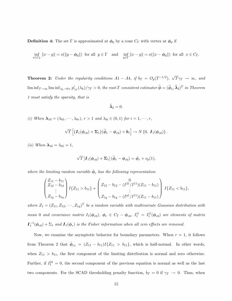
Definition 4: The set Γ is approximated at φ0 by a cone CΓ with vertex at φ0 if

infx∈CΓ

‖x − y‖ = o(‖y − φ0‖) for all y ∈ Γ and infy∈Γ

‖x − y‖ = o(‖x − φ0‖) for all x ∈ CΓ.

Theorem 2: Under the regularity conditions A1 − A4, if bT = Op(T−1/2),

√TγT → ∞, and

lim infT→∞ lim infλk→0+ p′γT(λk)/γT > 0, the root-T consistent estimator φ = (φ1, λ2)

T in Theorem

1 must satisfy the sparsity, that is

λ2 = 0.

(i) When λ10 = (λ01, · · · , λ0r), r > 1 and λ0i ∈ (0, 1) for i = 1, · · · , r,

√T[{I1(φr0) + Σ1}(φr − φr0) + b1

]→ N {0, I1(φr0)} .

(ii) When λ10 = λ01 = 1,

√T [I1(φr0) + Σ1] (φr − φr0) = φr + op(1),

where the limiting random variable φr has the following representation

Z11 − b11

Z12 − b12...

Z1q − b1q

I{Z11 > b11} +

0Z12 − b12 − (I21/I11)(Z11 − b11)

...Z1q − b1q − (Iq1/I11)(Z11 − b11)

I{Z11 < b11},

where Z1 = (Z11, Z12, · · · , Z1q)T be a random variable with multivariate Gaussian distribution with

mean 0 and covariance matrix I1(φr0), φr ∈ CΓ − φr0, Iij1 = Iij

1 (φr0) are elements of matrix

I−11 (φr0) + Σ1 and I1(φr) is the Fisher information when all zero effects are removed.

Now, we examine the asymptotic behavior for boundary parameters. When r = 1, it follows

from Theorem 2 that φr1 = (Z11 − b11)I{Z11 > b11}, which is half-normal. In other words,

when Z11 > b11, the first component of the limiting distribution is normal and zero otherwise.

Further, if I211 = 0, the second component of the previous equation is normal as well as the last

two components. For the SCAD thresholding penalty function, bT = 0 if γT → 0. Thus, when

15

√TγT → ∞, by Theorem 2, the corresponding penalized likelihood estimators preserve the oracle

property and perform as well as the maximum likelihood estimators for estimating λ1 if we would

know λ2 = 0 in advance.

Remark 4: We comment that all the asymptotic results in the above theorems would hold true

for time series context with a change of the asymptotic variance. For details, see Cai and Wang

(2008) for a more general setting under time series context.

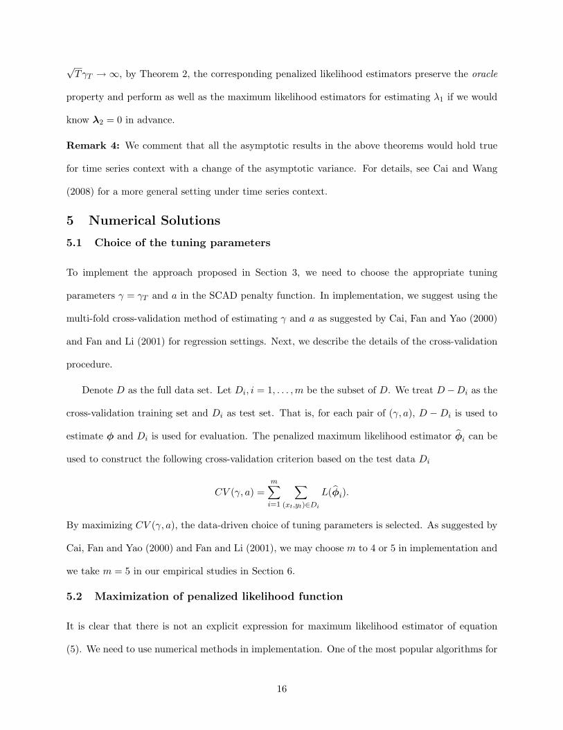
5 Numerical Solutions

5.1 Choice of the tuning parameters

To implement the approach proposed in Section 3, we need to choose the appropriate tuning

parameters γ = γT and a in the SCAD penalty function. In implementation, we suggest using the

multi-fold cross-validation method of estimating γ and a as suggested by Cai, Fan and Yao (2000)

and Fan and Li (2001) for regression settings. Next, we describe the details of the cross-validation

procedure.

Denote D as the full data set. Let Di, i = 1, . . . , m be the subset of D. We treat D −Di as the

cross-validation training set and Di as test set. That is, for each pair of (γ, a), D − Di is used to

estimate φ and Di is used for evaluation. The penalized maximum likelihood estimator φi can be

used to construct the following cross-validation criterion based on the test data Di

CV (γ, a) =m∑

i=1

∑

(xt,yt)∈Di

L(φi).

By maximizing CV (γ, a), the data-driven choice of tuning parameters is selected. As suggested by

Cai, Fan and Yao (2000) and Fan and Li (2001), we may choose m to 4 or 5 in implementation and

we take m = 5 in our empirical studies in Section 6.

5.2 Maximization of penalized likelihood function

It is clear that there is not an explicit expression for maximum likelihood estimator of equation

(5). We need to use numerical methods in implementation. One of the most popular algorithms for

16

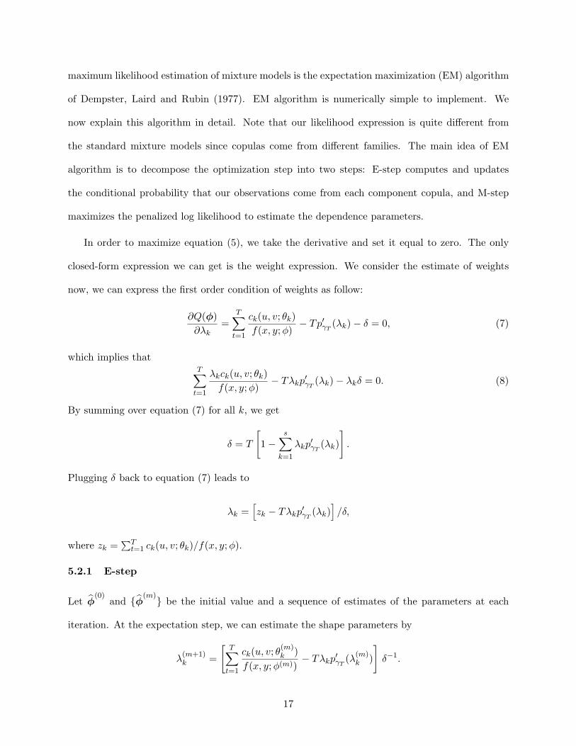
maximum likelihood estimation of mixture models is the expectation maximization (EM) algorithm

of Dempster, Laird and Rubin (1977). EM algorithm is numerically simple to implement. We

now explain this algorithm in detail. Note that our likelihood expression is quite different from

the standard mixture models since copulas come from different families. The main idea of EM

algorithm is to decompose the optimization step into two steps: E-step computes and updates

the conditional probability that our observations come from each component copula, and M-step

maximizes the penalized log likelihood to estimate the dependence parameters.

In order to maximize equation (5), we take the derivative and set it equal to zero. The only

closed-form expression we can get is the weight expression. We consider the estimate of weights

now, we can express the first order condition of weights as follow:

∂Q(φ)

∂λk=

T∑

t=1

ck(u, v; θk)

f(x, y; φ)− Tp′γT

(λk) − δ = 0, (7)

which implies thatT∑

t=1

λkck(u, v; θk)

f(x, y; φ)− Tλkp

′γT

(λk) − λkδ = 0. (8)

By summing over equation (7) for all k, we get

δ = T

[1 −

s∑

k=1

λkp′γT

(λk)

].

Plugging δ back to equation (7) leads to

λk =[zk − Tλkp

′γT

(λk)]/δ,

where zk =∑T

t=1 ck(u, v; θk)/f(x, y; φ).

5.2.1 E-step

Let φ(0)

and {φ(m)} be the initial value and a sequence of estimates of the parameters at each

iteration. At the expectation step, we can estimate the shape parameters by

λ(m+1)k =

[T∑

t=1

ck(u, v; θ(m)k )

f(x, y; φ(m))− Tλkp

′γT

(λ(m)k )

]δ−1.

17

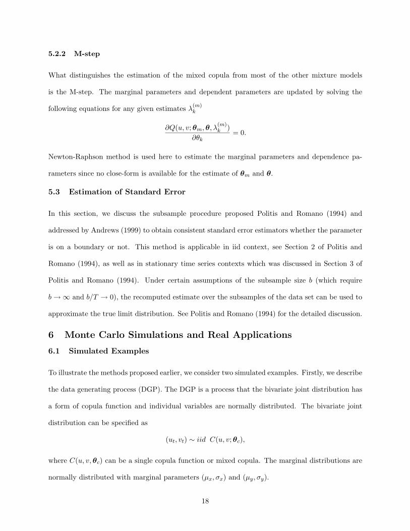
5.2.2 M-step

What distinguishes the estimation of the mixed copula from most of the other mixture models

is the M-step. The marginal parameters and dependent parameters are updated by solving the

following equations for any given estimates λ(m)k

∂Q(u, v; θm, θ, λ(m)k )

∂θk= 0.

Newton-Raphson method is used here to estimate the marginal parameters and dependence pa-

rameters since no close-form is available for the estimate of θm and θ.

5.3 Estimation of Standard Error

In this section, we discuss the subsample procedure proposed Politis and Romano (1994) and

addressed by Andrews (1999) to obtain consistent standard error estimators whether the parameter

is on a boundary or not. This method is applicable in iid context, see Section 2 of Politis and

Romano (1994), as well as in stationary time series contexts which was discussed in Section 3 of

Politis and Romano (1994). Under certain assumptions of the subsample size b (which require

b → ∞ and b/T → 0), the recomputed estimate over the subsamples of the data set can be used to

approximate the true limit distribution. See Politis and Romano (1994) for the detailed discussion.

6 Monte Carlo Simulations and Real Applications

6.1 Simulated Examples

To illustrate the methods proposed earlier, we consider two simulated examples. Firstly, we describe

the data generating process (DGP). The DGP is a process that the bivariate joint distribution has

a form of copula function and individual variables are normally distributed. The bivariate joint

distribution can be specified as

(ut, vt) ∼ iid C(u, v; θc),

where C(u, v, θc) can be a single copula function or mixed copula. The marginal distributions are

normally distributed with marginal parameters (µx, σx) and (µy, σy).

18

Our candidate copula families include four commonly used copulas: Gaussian, Clayton, Gumbel,

and Frank copulas. The Gaussian copula is widely used in financial fields and has symmetric

dependence in both tails of the distribution. Similarly, variables drawn from the Frank copula

also exhibit symmetric dependence in both tails. However, compared to the Gaussian copula,

dependence in the Frank copula is weaker in both tails and stronger in the center of the distribution,

as is evident from the fanning out in the tails. This suggests that the Frank copula is best suited

for applications in which tail dependence is relatively weak. In contrast to the Gaussian and Frank

copulas, the Clayton and Gumbel copulas exhibit asymmetric dependence. Clayton dependence is

strong in the left tail. The implication is that the Clayton copula is best suited for applications in

which two variables are likely to decrease together. On the other hand, the Gumbel copula exhibits

strong right tail dependence. Consequently, as is well-known, Gumbel is an appropriate modeling

choice when two variables are likely to simultaneously increase. The simulation results show that

the right copula can be selected although some of them have the same type of dependence structure.

The mixed copula based on the candidate copulas can be written as:

C(u, v; θc) = λ1CGau(u, v; θ1) + λ2CCla(u, v; θ2) + λ3CGum(u, v; θ3) + λ4CFra(u, v; θ4). (9)

Example 1: In this example, we consider the case that the joint distribution can be expressed by

a single copula function. The marginal distributions are Gaussian with parameters (µx, σx) and

(µy, σy) with values given in Table 1. Three sample sizes, 400, 700, and 1000, are considered and

the observations are simulated from single Gaussian copula by following the GDP proposed above

and the penalized maximum likelihood estimators are estimated. The simulation is repeated 100

times. The same procedures are performed for the other three copulas: Clayton, Gumbel, and

Frank. Thus, the jth model in this example has the form of equation (9) with λj = 1 and λi = 0

for all i 6= j.

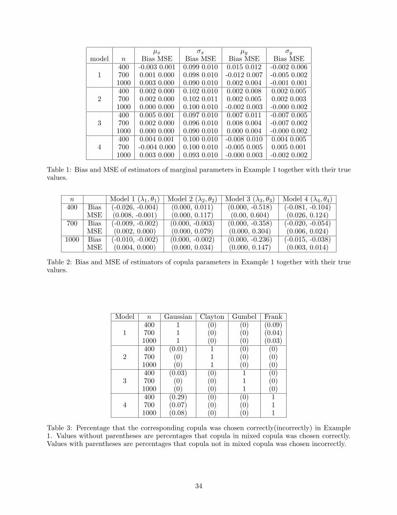
The simulated results are summarized in Tables 1, 2, 3, and 4. If the estimated weight of the

copula component is not zero, this copula component is selected, otherwise it is removed from

the mixed copula. In Table 3, the values without parentheses correspond to the percentages that

19

correct copulas are chosen, i.e., to the number of replications out of 100 when λj = 1 and λj 6= 0.

The values with parentheses correspond to the percentages that copulas are selected incorrectly,

i.e., to the number of replications out of 100 when λj 6= 0, but actually λj = 0. Tables 1 and

2 show the true values of the marginal parameters and dependence parameters from the copula,

biases and MSEs of the penalization maximum likelihood estimators. It shows clearly that the bias

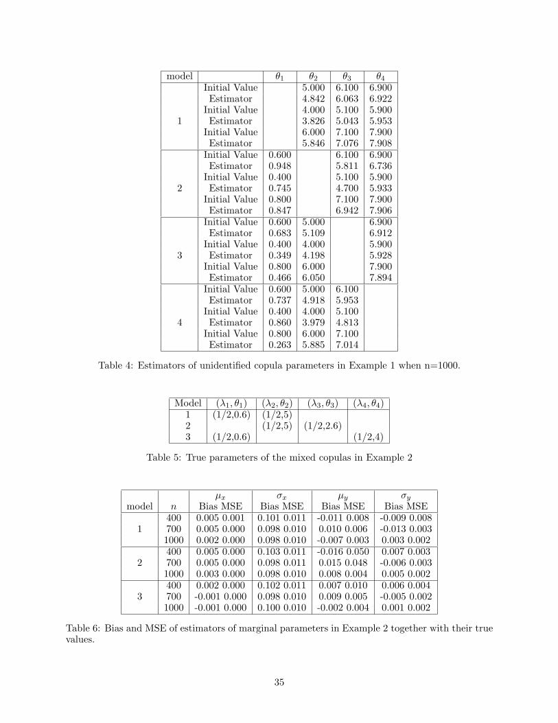
becomes smaller when the sample size is getting larger. Table 4 shows the initial values and the

estimated values of unidentified parameters and we can find the estimators converge to the initial

values. In other words, the penalized likelihood estimate of an unidentified parameter converges to

an arbitrary value. This is in line with our theory.

We can observe that performance of proposed method is good for choosing an appropriate copula

from a mixed model. For each model, we have the 100% of chance to choose the correct copula

function from which each data point is drawn. The percentage that incorrect copula is selected is

small. For the Gaussian copula, only 3% of chance to select Frank copula when n = 1000 and 8%

of chance to choose the Gaussian copula for those data points generated from the Frank copula.

This is not surprising because the Frank and Gaussian copulas have the same type of dependence

structure as that it is not easy to distinguish them.

Example 2: Now we consider the performance of the estimators when the joint distribution has

a form of mixed copula. We use the same marginal parameter values as those in Example 1. We

consider several mixed copulas with two components. The true values of parameters for mixed

copula are given in Table 5. We generate the data values for each mixed copula for three different

sample sizes: 400, 700, and 1000, thus the penalized maximum likelihood estimators are estimated.

We repeat this experiment 100 times for each model.

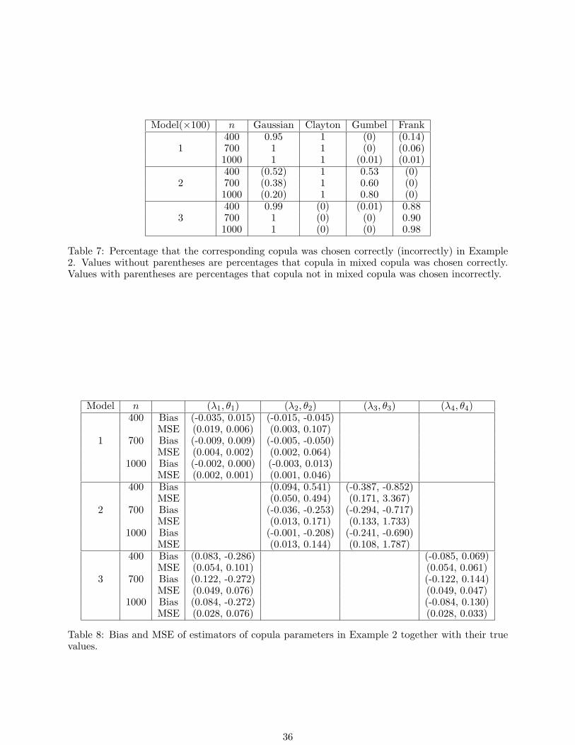
The simulation results are presented in Tables 6, 7, 8, and 9. Same as the format of Table 3,

Table 7 shows the percentages corresponding to the correct selected copula and incorrect selected

copula. Tables 6 and 8 display the true values of the marginal parameters and dependence param-

eters from the copula, biases and MSEs of the penalization maximum likelihood estimators and

20

Table 9 shows the initial values and the estimators of unidentified parameters.

Models simulated in this example can capture different dependence structures. Let’s consider

the cases when n = 1000. Model 1 is a mixture of Gaussian and Clayton copulas and describes the

lower tail dependence. We can see that there is a large probability to select the appropriate copula

in Model 1. For Model 2 which consists of Clayton and Gumbel copulas, Clayton is selected in all

replications and Gumbel is chosen 80 times out of 100 replications. The results from Model 3 are

very promising since Gaussian copula is selected 100 times and Frank copula is selected 98 times.

6.2 Empirical Examples

It is well known that the following real financial data are time series. As advocated in Remark 4, the

asymptotic theory developed in this paper holds true for time series too with a change of standard

error. To estimate the standard error consistently, we suggest using a subsampling technique in

Section 5.3, which is valid for time series context.

We conduct the empirical studies on the co-movement of returns among Asian markets, Chinese

markets and International markets in the following examples. The marginal distributions are

assumed to follow the t-distribution. The Kolmogorov-Smirnov (KS) tests are performed and the

results show that t-distribution is appropriate fit of the marginal distributions. The proposed

estimator is calculated and the standard errors are estimated based on the procedure suggested in

Section 5.3 with b = T 0.9, where T is the number of observations. Due to the limited space, we

only present the results of proposed estimate.

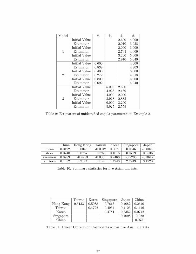
Example 3: The empirical analysis is carried out on returns on equity indices for six Asian

markets: China (CH), Hong Kong (HK), Taiwan (TW), Japan (JP), Singapore (SI), and South

Korea (KR). The data consists of 93 monthly observations from February 2000 to September

2007. The descriptive statistics are presented in Table 10. The correlation matrix between the six

markets are given in Table 11. The working model is model (9) for each pair. That is, a mixed

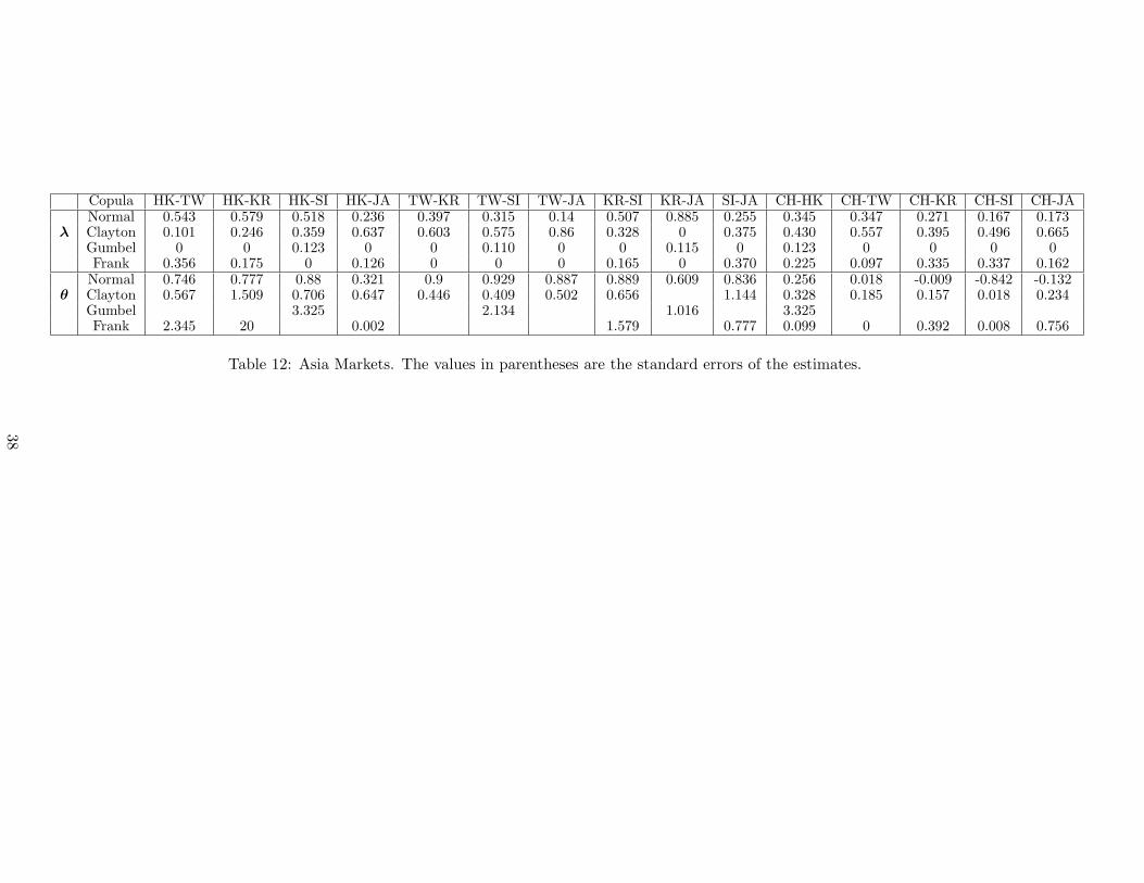
copula contains four well known copulas: Gaussian, Clayton, Gumbel, and Frank. Table 12 reports

21

the estimates of 15 models. We can notice several facts from Table 12. First, it can be seen clearly

that the dependence between Hong Kong and Singapore markets are strongest and that between

Singapore and China markets are weakest among all pairs. Further, only one pair, KR-JA, which

takes no weight on Clayton copula, and the other pairs put either zero weights or smaller weights

on Clayton copula than on Gumbel copula. This implies that the stock markets we consider have

bigger right tail dependence than left tail dependence. To explain this asymmetry, one hypothesis

is that investors are more sensitive to bad news than good news in other markets. When a crash

takes place in a foreign market, investors in domestic markets tend to pay much attention on it and

may result in some actions. These actions may pull the domestic market down. In the contrary,

people may not pay too much attention on the boom of another market. Moreover, 12 out of 15

pairs put larger weights on Gaussian than Frank copula. This finding suggests that the dependence

structure for both markets are more likely Gaussian type. That is, it is less possible that the

strongest dependence is centered in the middle of the distribution. Finally, ten pairs take more

weight on Clayton than Gaussian or Frank copula. We can conclude that the left tail dependence

describes the dependence structure best in our data set.

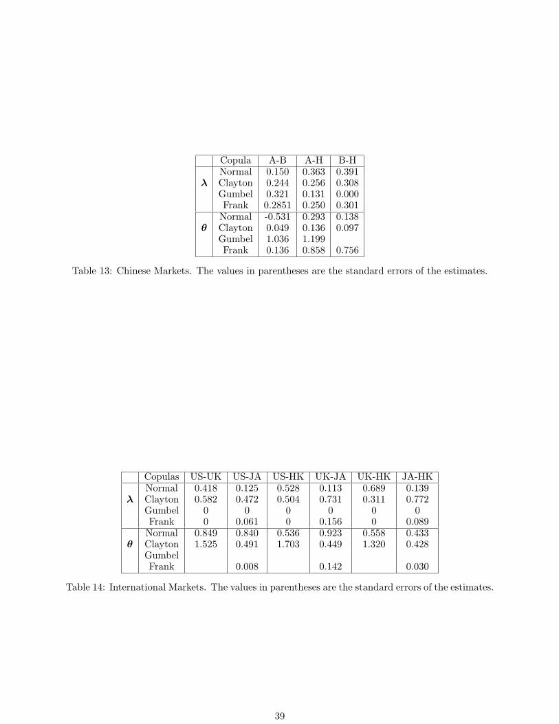
Example 4: We consider the Chinese markets A, B, and H daily indices and study their correlation

structures. Data period is from January 7, 2002 to September 12, 2007. The estimation results are

displayed in Table 13. We summarize several findings from the results: A index and B index are

more likely to boom together, A index and H index are more likely to crash together, and B index

and H index are more likely to crash together. We conclude that H may be in the lead position

such that the decrease in H index results in the decrease in A and B indices.

Example 5: We consider four stock market indices, S&P500 (US), FTSE 100 (UK), Nikkei (Japan),

and Hang Seng (Hong Kong). The data set is monthly returns from January 1987 to February 2007

and includes total 242 observations. Table 14 reports the estimates of models. Note that the weights

on Gumbel copula are zeros for all the pairs which indicates that no right tail dependence appears

for all pairs. All the pairs can be detected the left tail dependence which means that any two

22

different markets crash together. Hu (2003) proposed to use the Gaussian, Gumbel, and Survival

Gumbel mixture model to model the correlation structure among these four markets. The above

two findings we have are similar to the results of Hu (2003). But our results show somewhat the

Gaussian type of dependence which is in contrast to that in Hu (2003), who generally found a

weight of close to 0 on the Gaussian copula. This suggests that our method detects both linear

and nonlinear dependence, while Hu (2003) detected only nonlinear dependence.

7 Proofs of Theorems

In this section, we present the detailed proofs of Theorems 1 and 2.

Proof of Theorem 1: For any fixed point φ0 ∈ Γ0, let Bε(φ0) be an open ball of radius ε centered

at φ0. We know φ0 = (φTI0, θ

∗T2 )T , φI0 corresponds to the true values of the parameters and it is

unique for all the φ0, but the values of θ∗2 are different for different points φ0. Therefore, in order

to show that

φI −→ φI0, in probability,

and

θ2 −→ θ∗2, in probability,

it is sufficient to show that, for fixed point φ0,

Q(φ) < Q(φ0), in probability,

for any sufficiently small ε > 0 at all points φ on the surface of intersection of Bε(φ) and Γ. That

is, there exists a local maximum in the interior of Bε(φ).

Q(φ) − Q(φ0) = [L(φ) − L(φ0)] − Ts∑

k=1

[pγT(λk) − pγT

(λ0k)] + δs∑

k=1

[λk − λ0k]

≡ I1 − I2 + I3.

Applying Taylor’s expansion to L(φ) at point φ0, we have

I1 =

[∂L(φ0)

∂φ

]T(φ − φ0) +

1

2(φ − φ0)

T ∂2L(φ0)

∂φ∂φT(φ − φ0)

23

+1

6

∂

∂φ

[(φ − φ0)

T ∂2L(φ∗)

∂φ∂φT(φ − φ0)

](φ − φ0)

≡ I11 + I12 + I13,

where φ∗ lies between φ and φ0. By the law of large numbers,

1

T

∂L(φ0)

∂φ→ 0 in probability,

then, for any given ε,

∣∣∣∣1T

∂L(φ0)

∂φ

∣∣∣∣ < ε2. Thus,

∣∣∣∣1

TI11

∣∣∣∣ <p∑

j=1

ε2(φj − φ0j(φj)) = pε3.

Next, we consider I12. It is easy to see that

1

TI12 =

1

2T(φ − φ0)

T

[∂2L(φ0)

∂φ∂φT− E

{∂2L(φ0)

∂φ∂φT

}](φ − φ0)

+

[−1

2(φ − φ0)

T I(φ0)(φ − φ0)

]

≡ K1 + K2.

By the law of large numbers again, we have

1

T

∂2L(φ0)

∂φ∂φT=

1

TE

{∂2L(φ0)

∂φ∂φT

}+ op(1) = −I(φ0) + op(1).

Therefore, for any given ε, we have K1 < p2ε3. The second term K2 is a negative quadratic form of

(φ−φ0) and it is easy to show that K2 < −q1ε2, where q1 is the maximum eigenvalue of information

matrix I(φ0) and q1 < 0. Combining the first term K1 and second term K2, we obtain that there

exists a constant C > 0 such that

1

TI12 < −Cε2 in probability.

For I13, we have∣∣∣∣∣1

T

T∑

t=1

Mjkl(Xt, Yt)

∣∣∣∣∣ < 2 mjkl in probability.

Hence,by assumption A3,

∣∣∣∣1

TI13

∣∣∣∣ =

∣∣∣∣∣∣1

6T

p∑

j,k,l=1

∂3L(φ∗)

∂φj∂φk∂φl(φj − φ0j(φj))(φk − φ0k(φk))(φl − φ0l(φl))

∣∣∣∣∣∣

≤ 1

6Tε3

T∑

t=1

p∑

j,k,l=1

M2j,k,l(Xt, yt)

1/2

≤ 1

6p3ε3C = aε3,

24

where a = 16p3C. Thus, we get

1

TI1 < −Cε2 + (p + a)ε3. (10)

Now, we deal with the penalty term,

1

TI2 =

s∑

k=1

[pγT(λk) − pγT

(λ0k)]

=s∑

k=1

p′γT(λ0k)(λk − λ0k) +

1

2

s∑

k=1

p′′γT(λ0k)(λk − λ0k)

2{1 + o(1)}

≤ sε max1≤k≤s

{p′γT(λ0k)} +

1

2sε2 max

1≤k≤s{p′′γT

(λ0k)}{1 + o(1)}

≤ sεbT +1

2sε2 max

1≤k≤s{p′′γT

(λ0k)}{1 + o(1)},

where λ∗0k is between λk and λ0k. By the fact that bT → 0, the first term in 1

T I2 is less than sε3

for given ε. If max{p′′γT(λ0k)} goes to zero, the second term in 1

T I2 is bounded by 12sε3. That is

1

TI2 =

3

2sε3. (11)

By solving the Lagrange multiplier, we can find that δ = T [1 −∑sk=1 λkp

′γT

(λk)] and

1

TI3 = [1 −

s∑

k=1

λkp′γT

(λk)]s∑

k=1

(λk − λ0k) = 0. (12)

Combining the equations (10), (11), and (12), we have

1

T(I1 + I2 + I3) < −Cε2 + (p + a)ε3 +

3

2sε3.

Therefore,

Q(φ) < Q(φ0).

Now, we embark on the proof of the second part.

0 ≤ Q(φ) − Q(φ0)

= L(φ) − L(φ0) − Ts∑

k=1

[pγT(λk) − pγT

(λ0k)] + δs∑

k=1

(λk − λ0k)

=

[∂L(φ0)

∂φ

]T(φ − φ0) +

1

2(φ − φ0)

T

[∂2L(φ0)

∂φ∂φT

](φ − φ0) − T

s∑

k=1

p′γT(λ0k)(λk − λ0k)

25

−1

2T

s∑

k=1


2 +∥∥∥φ − φ0

∥∥∥3· Op(1)

=

[∂L(φ0)

∂φ

]T(φ − φ0) −

1

2T (φ − φ0)

T I(φ0)(φ − φ0) − Tb′(φ − φ0)

−1

2T (φ − φ0)

T Σ(φ − φ0) + ‖φ − φ0‖3 · Op(1).

Note that T−1/2 ∂L(φ0)

∂φ= Op(1) and ‖φ − φ0‖ = op(1). For each ε, there is a sequence cTε → 0

and a Kε such that with probability greater than 1 − ε,

∣∣∣∣1

T

∂L(φ0)

∂φ

∣∣∣∣ <Kε√

T

and

‖φ − φ0‖ < cTε.

Then, we have

0 ≤ 1

T(Q(φ) − Q(φ0))

≤ Kε√T‖φ − φ0‖ −

√sbT ‖φ − φ0‖ −

1

2(φ − φ0)

T (I(φ0) + Σ)(φ − φ0) + ‖φ − φ0‖3

≤ (Kε√

T−√

sbT )‖φ − φ0‖ −√

p

2max1≤i≤p

(hi)‖φ − φ0‖2 +1

2cTε‖φ − φ0‖2,

where hi is the eigenvalue of I(φ0) + Σ. By solving this inequality, we can get

∥∥∥φ − φ0

∥∥∥ <2(Kε/

√T +

√s bT )√

p max1≤i≤p(hi) + cTε< K∗

ε · (1/√

T + bT ).

This completes the proof of the theorem.

Lemma 1: Assume the conditions in Theorem 1, if lim infT→∞ lim infλk→0+ p′γT(λk)/γT > 0 and

√TγT → ∞, for any given φ such that ‖φ − φ0‖ = Op(T

−1/2) and any constant C, then,

Q(φ1, 0) ≥ Q(φ1, λ2) in probability.

Proof: It suffices to show that as n → ∞, for any φ2 satisfying ‖φ2 − φ20‖ = Op(T−1/2) and for

small εT = CT−1/2 and j = r + 1, . . . , s,

∂Q(φ)

∂λj< 0, for 0 < λj < εT .

26

By Taylor expansion, we have

∂Q(φ)

∂λj=

∂L(φ)

∂λj− Tp′γT

(λj) − δ

=∂L(φ0)

∂λj+

p∑

l=1

∂2L(φ0)

∂λj∂φl(φl − φl0) +

p∑

l=1

p∑

k=1

∂3L(φ∗)

∂λj∂φl∂φk(φl − φl0)(φk − φk0) − Tp′γT

(λj) − δ.(13)

It is easy to show that

1

T

∂L(φ0)

∂λj= Op(T

−1/2)

and

1

T

∂2L(φ0)

∂λj∂φl=

1

TE

[∂2L(φ0)

∂λj∂φl

]+ op(1).

For the second term in (13),

p∑

l=1

∂2L(φ0)

∂λj∂φl(φl − φl0)

=p∑

l=1

[∂2L(φ0)

∂λj∂φl− E

(∂2L(φ0)

∂λj∂φl

)](φl − φl0) +

p∑

l=1

E

(∂2L(φ0)

∂λj∂φl

)(φl − φl0)

≡ K1 + K2

By the assumption ‖φ − φ0‖ = Op(T−1/2), we have

|K2| =

∣∣∣∣∣Tp∑

l=1

I(φ0)(φl − φl0)

∣∣∣∣∣ ≤ TOp(T−1/2)

{ p∑

l=1

I2(φ0)

}1/2

.

Based on assumption (A4), we have

K2 = Op(√

T ).

As for the term K1, by the Cauchy-Schwarz inequality we have

|K1| ≤ ||φl − φl0| |

p∑

l=1

{∂2L(φ0)

∂λj∂φl− E

(∂2L(φ0)

∂λj∂φl

)}2

1/2

= Op(T−1/2)op(T ) = op(

√T ).

For the third term in (13), we have

p∑

l=1

∂3L(φ∗)

∂λj∂φl∂φk(φl − φl0)(φk − φk0)

=p∑

l=1

[∂3L(φ∗)

∂λj∂φl∂φk− E

(∂3L(φ∗)

∂λj∂φl∂φk

)](φl − φl0)(φk − φk0) +

p∑

l=1

E

(∂3L(φ∗)

∂λj∂φl∂φk

)(φl − φl0)(φk − φk0)

≡ K3 + K4.

27

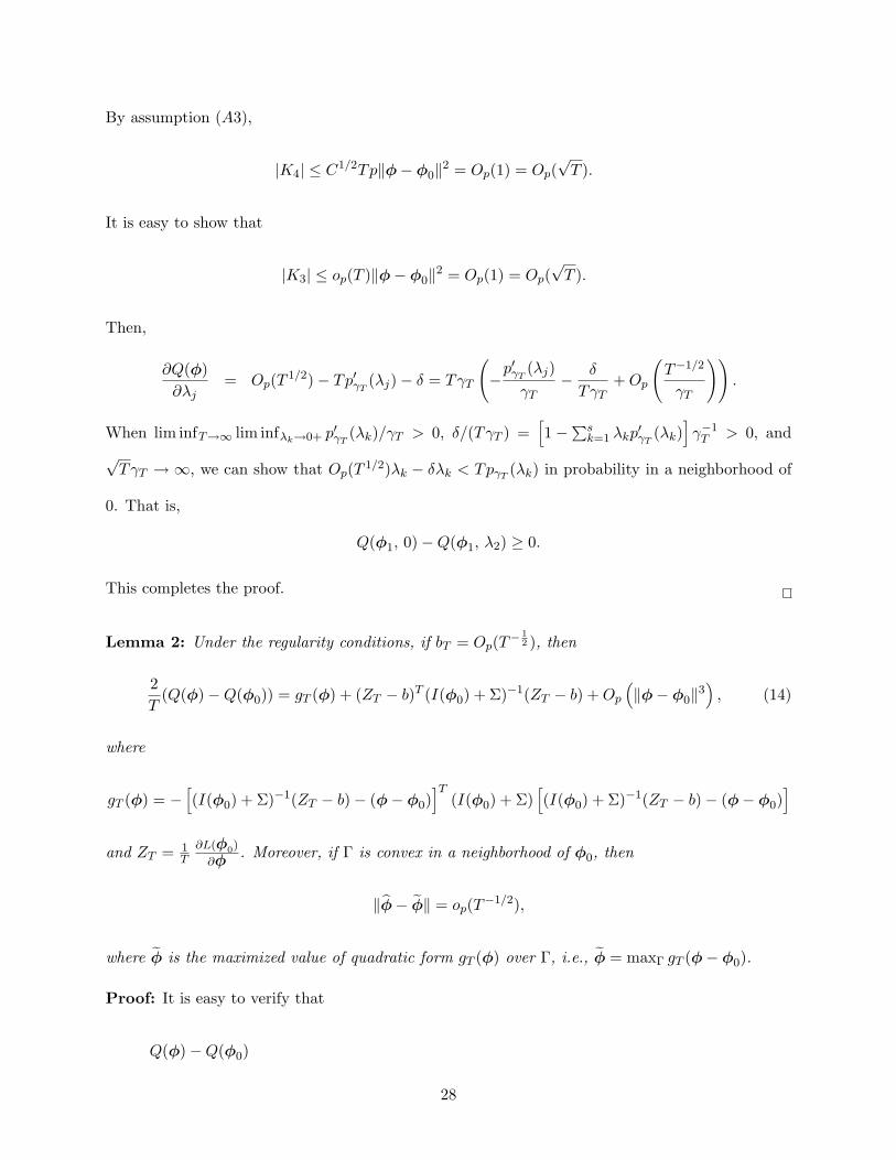
By assumption (A3),

|K4| ≤ C1/2Tp‖φ − φ0‖2 = Op(1) = Op(√

T ).

It is easy to show that

|K3| ≤ op(T )‖φ − φ0‖2 = Op(1) = Op(√

T ).

Then,

∂Q(φ)

∂λj= Op(T

1/2) − Tp′γT(λj) − δ = TγT

(−

p′γT(λj)

γT− δ

TγT+ Op

(T−1/2

γT

)).

When lim infT→∞ lim infλk→0+ p′γT(λk)/γT > 0, δ/(TγT ) =

[1 −∑s

k=1 λkp′γT

(λk)]γ−1

T > 0, and

√TγT → ∞, we can show that Op(T

1/2)λk − δλk < TpγT(λk) in probability in a neighborhood of

0. That is,

Q(φ1, 0) − Q(φ1, λ2) ≥ 0.

This completes the proof.

Lemma 2: Under the regularity conditions, if bT = Op(T− 1

2 ), then

2

T(Q(φ) − Q(φ0)) = gT (φ) + (ZT − b)T (I(φ0) + Σ)−1(ZT − b) + Op

(‖φ − φ0‖3

), (14)

where

gT (φ) = −[(I(φ0) + Σ)−1(ZT − b) − (φ − φ0)

]T(I(φ0) + Σ)

[(I(φ0) + Σ)−1(ZT − b) − (φ − φ0)

]

and ZT = 1T

∂L(φ0)

∂φ. Moreover, if Γ is convex in a neighborhood of φ0, then

‖φ − φ‖ = op(T−1/2),

where φ is the maximized value of quadratic form gT (φ) over Γ, i.e., φ = maxΓ gT (φ − φ0).

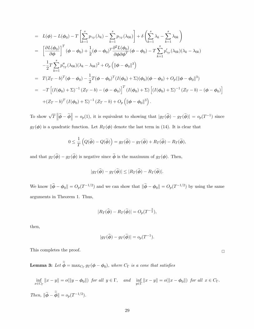
Proof: It is easy to verify that

Q(φ) − Q(φ0)

28

= L(φ) − L(φ0) − T

[s∑

k=1

pγT(λk) −

s∑

k=1

pγT(λ0k)

]+ δ

(s∑

k=1

λk −s∑

k=1

λ0k

)

=

[∂L(φ0)

∂φ

]T(φ − φ0) +

1

2(φ − φ0)

T ∂2L(φ0)

∂φ∂φT(φ − φ0) − T

s∑

k=1

p′γT(λ0k)(λk − λ0k)

−1

2T

s∑

k=1


2 + Op

(‖φ − φ0‖3

)

= T (ZT − b)T (φ − φ0) −1

2T (φ − φ0)

T (I(φ0) + Σ)(φ0)(φ − φ0) + Op(‖φ − φ0‖3)

= −T[(I(φ0) + Σ)−1 (ZT − b) − (φ − φ0)

]T(I(φ0) + Σ)

[(I(φ0) + Σ)−1 (ZT − b) − (φ − φ0)

]

+(ZT − b)T (I(φ0) + Σ)−1 (ZT − b) + Op

(‖φ − φ0‖3

).

To show√

T∥∥∥φ − φ

∥∥∥ = op(1), it is equivalent to showing that |gT (φ) − gT (φ)| = op(T−1) since

gT (φ) is a quadratic function. Let RT (φ) denote the last term in (14). It is clear that

0 ≤ 1

T

(Q(φ) − Q(φ)

)= gT (φ) − gT (φ) + RT (φ) − RT (φ),

and that gT (φ) − gT (φ) is negative since φ is the maximum of gT (φ). Then,

|gT (φ) − gT (φ)| ≤ |RT (φ) − RT (φ)|.

We know ‖φ − φ0‖ = Op(T−1/2) and we can show that ‖φ − φ0‖ = Op(T

−1/2) by using the same

arguments in Theorem 1. Thus,

|RT (φ) − RT (φ)| = Op(T− 3

2 ),

then,

|gT (φ) − gT (φ)| = op(T−1).


Lemma 3: Let˜φ = maxCΓ

gT (φ − φ0), where CΓ is a cone that satisfies

infx∈CΓ

‖x − y‖ = o(‖y − φ0‖) for all y ∈ Γ, and infy∈Γ

‖x − y‖ = o(‖x − φ0‖) for all x ∈ CΓ.

Then, ‖φ − ˜φ‖ = op(T

−1/2).

29

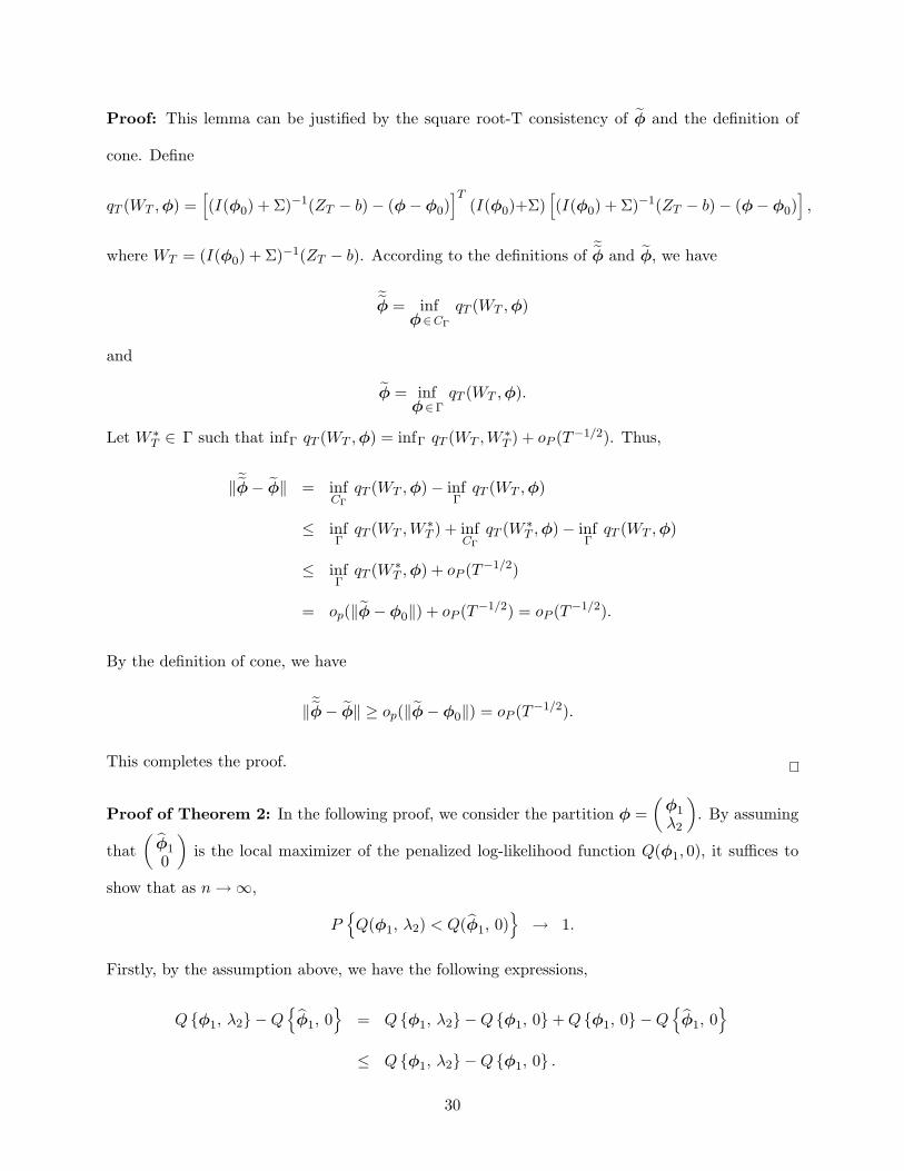
Proof: This lemma can be justified by the square root-T consistency of φ and the definition of

cone. Define

qT (WT , φ) =[(I(φ0) + Σ)−1(ZT − b) − (φ − φ0)

]T(I(φ0)+Σ)

[(I(φ0) + Σ)−1(ZT − b) − (φ − φ0)

],

where WT = (I(φ0) + Σ)−1(ZT − b). According to the definitions of˜φ and φ, we have

˜φ = inf

φ∈CΓ

qT (WT , φ)

and

φ = infφ∈Γ

qT (WT , φ).

Let W ∗T ∈ Γ such that infΓ qT (WT , φ) = infΓ qT (WT , W ∗

T ) + oP (T−1/2). Thus,

‖ ˜φ − φ‖ = infCΓ

qT (WT , φ) − infΓ

qT (WT , φ)

≤ infΓ

qT (WT , W ∗T ) + inf

CΓ

qT (W ∗T , φ) − inf

ΓqT (WT , φ)

≤ infΓ

qT (W ∗T , φ) + oP (T−1/2)

= op(‖φ − φ0‖) + oP (T−1/2) = oP (T−1/2).

By the definition of cone, we have

‖ ˜φ − φ‖ ≥ op(‖φ − φ0‖) = oP (T−1/2).


Proof of Theorem 2: In the following proof, we consider the partition φ =

(φ1λ2

). By assuming

that

(φ10

)is the local maximizer of the penalized log-likelihood function Q(φ1, 0), it suffices to

show that as n → ∞,

P{Q(φ1, λ2) < Q(φ1, 0)

}→ 1.

Firstly, by the assumption above, we have the following expressions,

Q {φ1, λ2} − Q{φ1, 0

}= Q {φ1, λ2} − Q {φ1, 0} + Q {φ1, 0} − Q

{φ1, 0

}

≤ Q {φ1, λ2} − Q {φ1, 0} .

30

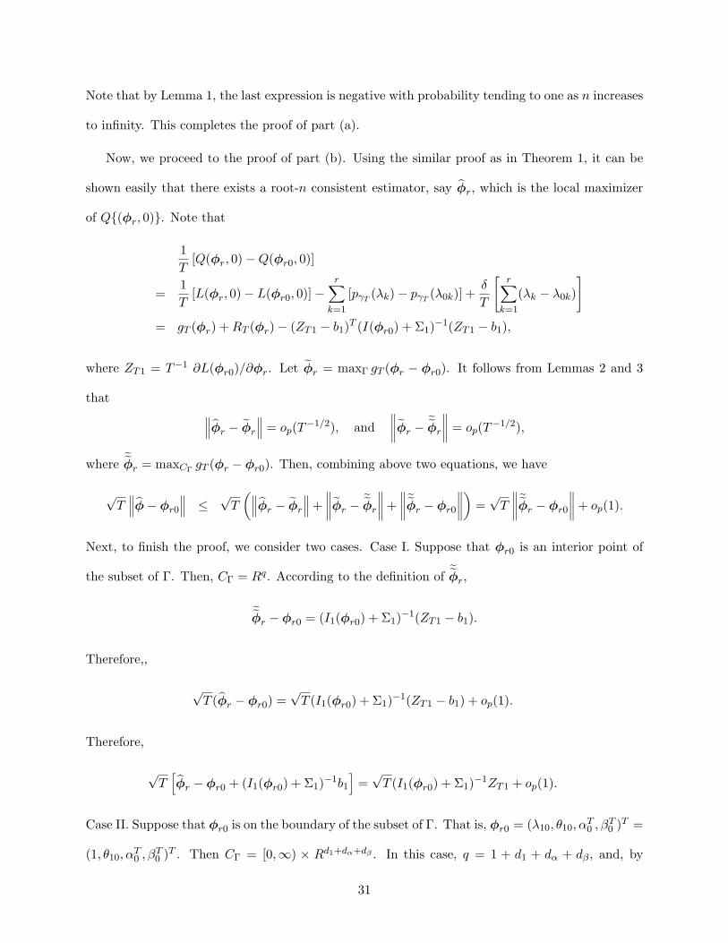
Note that by Lemma 1, the last expression is negative with probability tending to one as n increases

to infinity. This completes the proof of part (a).

Now, we proceed to the proof of part (b). Using the similar proof as in Theorem 1, it can be

shown easily that there exists a root-n consistent estimator, say φr, which is the local maximizer

of Q{(φr, 0)}. Note that

1

T[Q(φr, 0) − Q(φr0, 0)]

=1

T[L(φr, 0) − L(φr0, 0)] −

r∑

k=1

[pγT(λk) − pγT

(λ0k)] +δ

T

[r∑

k=1

(λk − λ0k)

]

= gT (φr) + RT (φr) − (ZT1 − b1)T (I(φr0) + Σ1)

−1(ZT1 − b1),

where ZT1 = T−1 ∂L(φr0)/∂φr. Let φr = maxΓ gT (φr − φr0). It follows from Lemmas 2 and 3

that∥∥∥φr − φr

∥∥∥ = op(T−1/2), and

∥∥∥∥φr −˜φr

∥∥∥∥ = op(T−1/2),

where˜φr = maxCΓ

gT (φr − φr0). Then, combining above two equations, we have

√T∥∥∥φ − φr0

∥∥∥ ≤√

T

(∥∥∥φr − φr

∥∥∥+

∥∥∥∥φr −˜φr

∥∥∥∥+

∥∥∥∥˜φr − φr0

∥∥∥∥)

=√

T

∥∥∥∥˜φr − φr0

∥∥∥∥+ op(1).

Next, to finish the proof, we consider two cases. Case I. Suppose that φr0 is an interior point of

the subset of Γ. Then, CΓ = Rq. According to the definition of˜φr,

˜φr − φr0 = (I1(φr0) + Σ1)

−1(ZT1 − b1).

Therefore,,

√T (φr − φr0) =

√T (I1(φr0) + Σ1)

−1(ZT1 − b1) + op(1).

Therefore,

√T[φr − φr0 + (I1(φr0) + Σ1)

−1b1

]=

√T (I1(φr0) + Σ1)

−1ZT1 + op(1).

Case II. Suppose that φr0 is on the boundary of the subset of Γ. That is, φr0 = (λ10, θ10, αT0 , βT

0 )T =

(1, θ10, αT0 , βT

0 )T . Then CΓ = [0,∞) × Rd1+dα+dβ . In this case, q = 1 + d1 + dα + dβ , and, by

31

maximizing the quadratic form gT (φr) over CΓ,˜φr has the representation as

√T [I1(φr0) + Σ1] (

˜φr − φr0) = φr + op(1),

where the limiting random variable φr has the following representation

Z11 − b11

Z12 − b12...

Z1q − b1q

I{Z11 > b11} +

0Z12 − b12 − (I21/I11)(Z11 − b11)

...Z1q − b1q − (Iq1/I11)(Z11 − b11)

I{Z11 < b11},

where Z1 = (Z11, Z12, · · · , Z1q)T be a random variable with multivariate Gaussian distribution

with mean 0 and covariance matrix I1(φr0), φr ∈ CΓ − φr0, Iij1 = Iij

1 (φr0) are elements of matrix

I−11 (φr0)+Σ1 and I1(φr) is the Fisher information when all zero effects are removed. This completes

the proof.

References

Andrews, D. (1999). Estimation When a Parameter is on a Boundary, Econometrica, 67, 1341-1383.

Ang, A. and J. Chen (2002). Asymmetric Correlations of Equity Portfolios, Review of FinancialStudies, 63, 443-494.

Antoniadis, A. and J. Fan (2201). Regularization of Wavelets Approximations, Journal of theAmerican Statistical Association, 96, 939-967.

Bouye, E., V. Durrleman, A. Nikeghbali, G. Riboulet and T. Roncalli (2001). Copulas: an OpenField for Risk Management, Discussion paper, Groupe de Recherche Operationnelle, CreditLyonnais.

Cai, Z., J. Fan and Q. Yao (2000). Functional-Coefficient Regression Models for Nonlinear TimeSeries, Journal of the American Statistical Association, 95, 941-956.

Cai, Z. and X. Wang (2008). Selection of Finite Mixture Distribution, in preparation.

Chen, J. and A. Khalili (2006). Order Selection in Finite Mixture Models, Working Paper, De-partment of Statistics and Actuarial Science, University of Waterloo.

Chen, X., Y. Fan and A. Patton (2003), Simple Tests for Models of Dependence between FinancialTime Series: with Applications to US Equity Returns and Exchange Rates, Mimeo.

Cherubini, U., W. Vecchiato and E. Luciano (2004). Copula Methods in Finance, Wiley, NewYork.

Chollete, L., V. Pena and C. Lu (2005). Comovement of International Financial Markets, WorkingPaper, Columbia University.

32

Dempster, A.P., N.M. Laird and D.B. Rubin (1977). Maximum Likelihood from Incomplete Datavia the EM Algorithm, Journal of the Royal Statistical Society, Series B, 39, 1-38.

Donoho, D. L. and I. M. Johnstone (1994). Ideal Spatial Adaptation by Wavelet Shrinkage,Biometrika, 81, 425-455.

Embrechts, P., F. Lindskog and A.J. McNell (2003). Modelling Dependence with Copulas andApplications to Risk Management, Handbook of Heavy Tailed Distributions in Finance Ed:S. Rachev, Elsevier, Chapter 8, 329-384.

Fan, J. (1997). Comments on “Wavlets in Statistics: A Review” by A. Antoniadis, Journal of theItalian Statistical Association, 6, 131-138.

Fan, J. and R. Li (2001). Variable Selection via Nonconcave Penalized Likelihood and its OracleProperties, Journal of the American Statistical Association, 96, 1348-1360.

Fan, J. and H. Peng (2004). Nonconcave Penalized Likelihood with Diverging Number of Param-eters, The Annals of Statistics, 32, 928-961.

Frank, I.E. and Friedman, J.H. (1993). A Statistical View of some Chemometrics RegressionTools, Technometrics, 35, 109-148.

Fu, W.J. (1998). Penalized Regression: the Bridge Versus the LASSO, Journal of Computationaland Graphical Statistics, 7, 397-416.

Fermanian, J.-D. (2005). Goodness of Fit Tests for Copulas, Journal of Multivariate Analysis,95, 119-152.

Hu, L. (2003). Dependence Patterns Across Financial Markets: a Mixed Copula Approach, AppliedFinancial Economics, 16, 717-729.

Joe, H. (1997). Multivariate Models and Dependence Concepts, Chapman & Hall, London.

Li, D. (2000). On default Correlation: A Copula Function Approach, Journal of Fixed Income,9, 43-54.

Longin, F. and B. Solnik (2001). Extreme Correlation of International Equity Markets, Journalof Finance, 56, 649-676.

McLanchlan, G. and D. Peel (2000). Finite Mixture Models, Wiley, New York.

Nelsen, R.B. (1998). An Introduction to Copulas, Springer-Verlag, New York.

Politis, D.N. and J.P. Romano (1994). Large Sample Confidence Regions Based on Subsamplesunder Minimal Assumptions, Annals of Statistics, 22, 2031-2050.

Sklar, A. (1959). Fonctions de Repartition a n Dimensions et Leures Marges, Publications deL’Institut de Statistique de L’Universite de Paris, 8, 229-231.

Tibshirani, R.J. (1996). Regression Shrinkage and Selection via the Lasso, Journal of the RoyalStatistical Society, Series B, 58, 267-288.

33

µx σx µy σy

model n Bias MSE Bias MSE Bias MSE Bias MSE400 -0.003 0.001 0.099 0.010 0.015 0.012 -0.002 0.006

1 700 0.001 0.000 0.098 0.010 -0.012 0.007 -0.005 0.0021000 0.003 0.000 0.090 0.010 0.002 0.004 -0.001 0.001400 0.002 0.000 0.102 0.010 0.002 0.008 0.002 0.005

2 700 0.002 0.000 0.102 0.011 0.002 0.005 0.002 0.0031000 0.000 0.000 0.100 0.010 -0.002 0.003 -0.000 0.002400 0.005 0.001 0.097 0.010 0.007 0.011 -0.007 0.005

3 700 0.002 0.000 0.096 0.010 0.008 0.004 -0.007 0.0021000 0.000 0.000 0.090 0.010 0.000 0.004 -0.000 0.002400 0.004 0.001 0.100 0.010 -0.008 0.010 0.004 0.005

4 700 -0.004 0.000 0.100 0.010 -0.005 0.005 0.005 0.0011000 0.003 0.000 0.093 0.010 -0.000 0.003 -0.002 0.002

Table 1: Bias and MSE of estimators of marginal parameters in Example 1 together with their truevalues.

n Model 1 (λ1, θ1) Model 2 (λ2, θ2) Model 3 (λ3, θ3) Model 4 (λ4, θ4)400 Bias (-0.026, -0.004) (0.000, 0.011) (0.000, -0.518) (-0.081, -0.104)

MSE (0.008, -0.001) (0.000, 0.117) (0.00, 0.604) (0.026, 0.124)700 Bias (-0.009, -0.002) (0.000, -0.003) (0.000, -0.358) (-0.020, -0.054)

MSE (0.002, 0.000) (0.000, 0.079) (0.000, 0.304) (0.006, 0.024)1000 Bias (-0.010, -0.002) (0.000, -0.002) (0.000, -0.236) (-0.015, -0.038)

MSE (0.004, 0.000) (0.000, 0.034) (0.000, 0.147) (0.003, 0.014)

Table 2: Bias and MSE of estimators of copula parameters in Example 1 together with their truevalues.

Model n Gaussian Clayton Gumbel Frank400 1 (0) (0) (0.09)

1 700 1 (0) (0) (0.04)1000 1 (0) (0) (0.03)400 (0.01) 1 (0) (0)

2 700 (0) 1 (0) (0)1000 (0) 1 (0) (0)400 (0.03) (0) 1 (0)

3 700 (0) (0) 1 (0)1000 (0) (0) 1 (0)400 (0.29) (0) (0) 1

4 700 (0.07) (0) (0) 11000 (0.08) (0) (0) 1

Table 3: Percentage that the corresponding copula was chosen correctly(incorrectly) in Example1. Values without parentheses are percentages that copula in mixed copula was chosen correctly.Values with parentheses are percentages that copula not in mixed copula was chosen incorrectly.

34

model θ1 θ2 θ3 θ4

Initial Value 5.000 6.100 6.900Estimator 4.842 6.063 6.922

Initial Value 4.000 5.100 5.9001 Estimator 3.826 5.043 5.953











Table 4: Estimators of unidentified copula parameters in Example 1 when n=1000.

Model (λ1, θ1) (λ2, θ2) (λ3, θ3) (λ4, θ4)1 (1/2,0.6) (1/2,5)2 (1/2,5) (1/2,2.6)3 (1/2,0.6) (1/2,4)

Table 5: True parameters of the mixed copulas in Example 2

µx σx µy σy

model n Bias MSE Bias MSE Bias MSE Bias MSE400 0.005 0.001 0.101 0.011 -0.011 0.008 -0.009 0.008

1 700 0.005 0.000 0.098 0.010 0.010 0.006 -0.013 0.0031000 0.002 0.000 0.098 0.010 -0.007 0.003 0.003 0.002400 0.005 0.000 0.103 0.011 -0.016 0.050 0.007 0.003

2 700 0.005 0.000 0.098 0.011 0.015 0.048 -0.006 0.0031000 0.003 0.000 0.098 0.010 0.008 0.004 0.005 0.002400 0.002 0.000 0.102 0.011 0.007 0.010 0.006 0.004

3 700 -0.001 0.000 0.098 0.010 0.009 0.005 -0.005 0.0021000 -0.001 0.000 0.100 0.010 -0.002 0.004 0.001 0.002

Table 6: Bias and MSE of estimators of marginal parameters in Example 2 together with their truevalues.

35

Model(×100) n Gaussian Clayton Gumbel Frank400 0.95 1 (0) (0.14)

1 700 1 1 (0) (0.06)1000 1 1 (0.01) (0.01)400 (0.52) 1 0.53 (0)

2 700 (0.38) 1 0.60 (0)1000 (0.20) 1 0.80 (0)400 0.99 (0) (0.01) 0.88

3 700 1 (0) (0) 0.901000 1 (0) (0) 0.98

Table 7: Percentage that the corresponding copula was chosen correctly (incorrectly) in Example2. Values without parentheses are percentages that copula in mixed copula was chosen correctly.Values with parentheses are percentages that copula not in mixed copula was chosen incorrectly.

Model n (λ1, θ1) (λ2, θ2) (λ3, θ3) (λ4, θ4)400 Bias (-0.035, 0.015) (-0.015, -0.045)

MSE (0.019, 0.006) (0.003, 0.107)1 700 Bias (-0.009, 0.009) (-0.005, -0.050)

MSE (0.004, 0.002) (0.002, 0.064)1000 Bias (-0.002, 0.000) (-0.003, 0.013)

MSE (0.002, 0.001) (0.001, 0.046)400 Bias (0.094, 0.541) (-0.387, -0.852)

MSE (0.050, 0.494) (0.171, 3.367)2 700 Bias (-0.036, -0.253) (-0.294, -0.717)

MSE (0.013, 0.171) (0.133, 1.733)1000 Bias (-0.001, -0.208) (-0.241, -0.690)

MSE (0.013, 0.144) (0.108, 1.787)400 Bias (0.083, -0.286) (-0.085, 0.069)

MSE (0.054, 0.101) (0.054, 0.061)3 700 Bias (0.122, -0.272) (-0.122, 0.144)

MSE (0.049, 0.076) (0.049, 0.047)1000 Bias (0.084, -0.272) (-0.084, 0.130)

MSE (0.028, 0.076) (0.028, 0.033)

Table 8: Bias and MSE of estimators of copula parameters in Example 2 together with their truevalues.

36

Model θ1 θ2 θ3 θ4

Initial Value 2.600 4.000Estimator 2.010 3.938

Initial Value 2.000 3.0001 Estimator 2.705 4.009








Table 9: Estimators of unidentified copula parameters in Example 2.

China Hong Kong Taiwan Korea Singapore Japanmean 0.0122 0.0045 -0.0012 0.0077 0.0046 -0.0020stdev 0.0740 0.0787 0.0769 0.1016 0.0779 0.0536

skewness 0.8789 -0.4253 -0.0061 0.2463 -0.2286 -0.3647kurtosis 0.1052 3.2174 0.5143 1.4943 2.2949 3.1228

Table 10: Summary statistics for five Asian markets.

Taiwan Korea Singapore Japan ChinaHong Kong 0.5133 0.5088 0.7613 0.4082 0.2640

Taiwan 0.4722 0.4934 0.4123 0.1146Korea 0.4781 0.5352 0.0742

Singapore 0.4098 -0.020China 0.075

Table 11: Linear Correlation Coefficients across five Asian markets.

37

Copula HK-TW HK-KR HK-SI HK-JA TW-KR TW-SI TW-JA KR-SI KR-JA SI-JA CH-HK CH-TW CH-KR CH-SI CH-JANormal 0.543 0.579 0.518 0.236 0.397 0.315 0.14 0.507 0.885 0.255 0.345 0.347 0.271 0.167 0.173

λ Clayton 0.101 0.246 0.359 0.637 0.603 0.575 0.86 0.328 0 0.375 0.430 0.557 0.395 0.496 0.665Gumbel 0 0 0.123 0 0 0.110 0 0 0.115 0 0.123 0 0 0 0Frank 0.356 0.175 0 0.126 0 0 0 0.165 0 0.370 0.225 0.097 0.335 0.337 0.162

Normal 0.746 0.777 0.88 0.321 0.9 0.929 0.887 0.889 0.609 0.836 0.256 0.018 -0.009 -0.842 -0.132θ Clayton 0.567 1.509 0.706 0.647 0.446 0.409 0.502 0.656 1.144 0.328 0.185 0.157 0.018 0.234

Gumbel 3.325 2.134 1.016 3.325Frank 2.345 20 0.002 1.579 0.777 0.099 0 0.392 0.008 0.756

Table 12: Asia Markets. The values in parentheses are the standard errors of the estimates.

38

Copula A-B A-H B-HNormal 0.150 0.363 0.391

λ Clayton 0.244 0.256 0.308Gumbel 0.321 0.131 0.000Frank 0.2851 0.250 0.301

Normal -0.531 0.293 0.138θ Clayton 0.049 0.136 0.097

Gumbel 1.036 1.199Frank 0.136 0.858 0.756

Table 13: Chinese Markets. The values in parentheses are the standard errors of the estimates.

Copulas US-UK US-JA US-HK UK-JA UK-HK JA-HKNormal 0.418 0.125 0.528 0.113 0.689 0.139

λ Clayton 0.582 0.472 0.504 0.731 0.311 0.772Gumbel 0 0 0 0 0 0Frank 0 0.061 0 0.156 0 0.089

Normal 0.849 0.840 0.536 0.923 0.558 0.433θ Clayton 1.525 0.491 1.703 0.449 1.320 0.428

GumbelFrank 0.008 0.142 0.030

Table 14: International Markets. The values in parentheses are the standard errors of the estimates.

39

selection of copulas with applications in...

Documents