selecting variables in multiple regression - statpower notes/variableselection.pdf · selecting...

Selecting Variables in Multiple Regression

James H. Steiger

Department of Psychology and Human DevelopmentVanderbilt University

James H. Steiger (Vanderbilt University) Selecting Variables in Multiple Regression 1 / 29

Selecting Variables in Multiple Regression1 Introduction

2 The Problem with Redundancy

Collinearity and Variances of Beta Estimates

3 Detecting and Dealing with Redundancy

4 Classic Selection Procedures

The Akaike Information Criterion (AIC)

The Bayesian Information Criterion(BIC)

Cross-Validation Based Criteria

An Example — The Highway Data

Forward Selection

Backward Elimination

Stepwise Regression

5 Computational Examples

6 Caution about Selection Methods


Introduction

Introduction

One problem that can arise in “exploratory” multiple regression studies is which predictorsfrom a set of potential predictor variables should be included in the multiple regressionanalysis, and in the ultimate prediction formula.In this module, we review some traditional and newer approaches to variable selection,pointing out some of the pitfalls involved in selecting a subset of variables to analyze.


The Problem with Redundancy

The Problem with Redundancy

A fundamental problem when one has several potential predictors is that some may belargely redundant with others.One result of such redundancy is called multicollinearity, which occurs when somepredictors are linear combinations of others (or nearly so), resulting in a covariance matrixof predictors that is singular, or nearly so.One outcome of multicollinearity is that parameter estimates become subject to wildsampling fluctuations, for theoretical reasons that we investigate on the next slide.


The Problem with Redundancy Collinearity and Variances of Beta Estimates

The Problem with RedundancyCollinearity and Variances of Beta Estimates

Suppose we have just two predictors, and the mean function is

E (Y |X1 = x1,X2 = x2) = β0 + β1X1 + β2X2 (1)

It can be shown that

Var(βj) =σ2

1− r212

1

SXjXj(2)

where r12 is the correlation between X1 and X2, and SXjXj =∑

i (xij − x j)2.

From the above formula, we can see that, as r212 approaches 1, these variances are greatlyinflated.


The Problem with Redundancy Collinearity and Variances of Beta Estimates

The Problem with RedundancyCollinearity and Variances of Beta Estimates

When the number of predictors exceeds 2, the previous result generalizes.Specifically, we have

Var(βj) =σ2

1− R2j

1

SXjXj(3)

where R2j is the squared multiple correlation between Xj and the other predictors.

It is easy to see why the quantity 1/(1− R2j ) is called the jth variance inflation factor, or

VIFj .


Detecting and Dealing with Redundancy


Simple multicollinearity may be detected in several ways. For example, one might examinethe correlation matrix to see if any predictors are highly correlated, and delete some.Examining the varimax-rotated principal component structure of a set of predictors willreveal more complex forms of multicollinearity, so long as the redundancy is linear.Principal component analysis will reveal uncorrelated variables that are linearcombinations of the original predictors, and which account for maximum possible variance.If there is a lot of redundancy, just a few principal components might be as effective.




In some cases, predictors may be redundant with each other, but the redundancy isnonlinear.Frank Harrell’s Hmisc package includes a function redun to detect such nonlinearredundancy and suggest variables that might be candidates for elimination.


Classic Selection Procedures


In this section, we review the classic variable selection procedures that have dominatedthe social sciences literature.These procedures are usually referred to as

1 Forward Selection2 Backward Elimination3 Stepwise Regression




The goal of variable selection is to divide a set of predictors in the columns of a matrix Xinto active and inactive terms.The number of partitions is 2k , which becomes quite large very quickly when k is evenmoderate.There are two fundamental issues:

1 Given a particular candidate for the active terms, what criterion should be used to comparethis candidate to other possible choices?

2 How do we deal computationally with the potentially huge number of comparisons that needto be made?




Originally, the criteria for model evaluation were purely statistical. In order to be added toa model, a variable had to be significant according to the classic partial F test, eitherwith a p-value below a certain “p to enter” value, or with an F statistic specified as the“F to enter” value (as in SPSS).More recently, attention has shifted to so-called “informational criteria,” which appear, atleast at first glance, to combine model fit with model complexity in assessing whether avariable should be added to a prediction formula.


Classic Selection Procedures The Akaike Information Criterion (AIC)

Classic Selection ProceduresThe Akaike Information Criterion (AIC)

Criteria for comparing various candidate subsets are based on the lack of fit of a modeland its complexity.Ignoring constants that are the same for every candidate subset, the AIC, or AkaikeInformation Criterion for a candidate C, is

AICC = n log(RSSC/n) + 2pC (4)

According to the Akaike criterion, the model with the smallest AIC is to be preferred.


Classic Selection Procedures The Bayesian Information Criterion(BIC)

Classic Selection ProceduresThe Bayesian Information Criterion(BIC)

The Schwarz Bayesian Informatin Criterion (BIC) is

BICC = n log(RSSC/n) + pC log(n) (5)


Classic Selection Procedures Cross-Validation Based Criteria

Classic Selection ProceduresCross-Validation Based Criteria

The major reason for employing fit indices that correct for complexity is because, forsample data, increasing the complexity of the model can never yield a higher RSS , andalmost always will yield a lower RSS , even when the increase in complexity yields no gainin prediction in the population.In genuine cross-validation, the sample is divided into two parts at random, a construction(or calibration) set and a validation set.The model is fit to the construction set and parameter estimates are obtained.That model with those parameter estimates is then used to predict the response variablein the validation set data.The RSS is used as a measure of fit, and is not corrected for complexity.




The PRESS measure is an attempt to assess the cross-validation capability of a modelbased on a single sample.For a particular model, for each observation,

compute fitted values from β based on all the data other than that observation.compute the squared difference between the response and the predicted values

These squared errors are summed up across the entire sample.




The resulting statistic, for model subset candidate XC is

PRESS =n∑

i=1

(yi − x′Ci βC(i)

)2(6)

PRESS can be computed as

PRESS =n∑

i=1

(eCi

1− hCii

)2

(7)

where eCi and hCii are, respectively, the residual and the leverage for the ith case in thesubset model.This index is relatively straightforward to compute in simple linear regression because ofthe above computational simplification, but this simplicity does not generalize to morecomplex models.


Classic Selection Procedures An Example — The Highway Data

Classic Selection ProceduresAn Example — The Highway Data

This example employs the highway accident data from ALR Section 8.2.The variables (including the response, log(Rate)), are described in ALR3 Table 10.5reproduced below.

218 VARIABLE SELECTION

Small values of AIC are preferred, so better candidate sets will have smaller RSSand a smaller number of terms pC . An alternative to AIC is the Bayes InformationCriterion, or BIC, given by Schwarz (1978),

BIC = n log(RSSC/n) + pC log(n) (10.8)

which provides a different balance between lack of fit and complexity. Once again,smaller values are preferred.

Yet a third criterion that balances between lack of fit and complexity is Mallows’Cp (Mallows, 1973), where the subscript p is the number of terms in candidateXC . This statistic is defined by

CpC = RSSCσ 2

+ 2pC − n (10.9)

where σ 2 is from the fit of (10.1). As with many problems for which many solutionsare proposed, there is no clear choice between the criteria for preferring a subsetmean function. There is an important similarity between all three criteria: if wefix the complexity, meaning that we consider only the choices XC with a fixednumber of terms, then all three will agree that the choice with the smallest valueof residual sum of squares is the preferred choice.

Highway Accident DataWe will use the highway accident data described in Section 7.2. The initial termswe consider include the transformations found in Section 7.2.2 and a few others andare described in Table 10.5. The response variable is, from Section 7.3, log(Rate).This mean function includes 14 terms to describe only n = 39 cases.

TABLE 10.5 Definition of Terms for the Highway Accident Data

Variable Description

log(Rate) Base-two logarithm of 1973 accident rate per million vehicle miles,the response

log(Len) Base-two logarithm of the length of the segment in mileslog(ADT) Base-two logarithm of average daily traffic count in thousandslog(Trks) Base-two logarithm of truck volume as a percent of the total volumeSlim 1973 speed limitLwid Lane width in feetShld Shoulder width in feet of outer shoulder on the roadwayItg Number of freeway-type interchanges per mile in the segmentlog(Sigs1) Base-two logarithm of (number of signalized interchanges per mile

in the segment + 1)/(length of segment)Acpt Number of access points per mile in the segmentHwy A factor coded 0 if a federal interstate highway, 1 if a principal

arterial highway, 2 if a major arterial, and 3 otherwise




We begin by fitting a model with all terms

> data(highway)

> a <- highway

> a$logADT <- logb(a$ADT,2)

> a$logTrks <- logb(a$Trks,2)

> a$logLen <- logb(a$Len,2)

> a$logSigs1 <- logb((a$Sigs*a$Len+1)/a$Len,2)

> a$logRate <- logb(a$Rate,2)

> # set the contrasts to the R default

> options(contrasts=c(factor="contr.treatment",ordered="contr.poly"))

> a$Hwy <- if(is.null(version$language) == FALSE) factor(a$Hwy,ordered=FALSE) else factor(a$Hwy)

> attach(a)

> names(a)

[1] "ADT" "Trks" "Lane" "Acpt" "Sigs" "Itg"

[7] "Slim" "Len" "Lwid" "Shld" "Hwy" "Rate"

[13] "logADT" "logTrks" "logLen" "logSigs1" "logRate"

> cols <- c(17,15,13,14,16,7,10,3,4,6,9,11)

> m1 <- lm(logRate ~ logLen+logADT+logTrks+logSigs1+Slim+Shld+

+ Lane+Acpt+Itg+Lwid+Hwy)




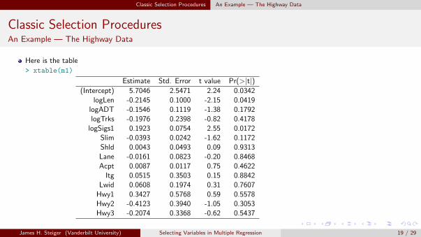
Here is the table

> xtable(m1)

Estimate Std. Error t value Pr(>|t|)(Intercept) 5.7046 2.5471 2.24 0.0342

logLen -0.2145 0.1000 -2.15 0.0419logADT -0.1546 0.1119 -1.38 0.1792logTrks -0.1976 0.2398 -0.82 0.4178

logSigs1 0.1923 0.0754 2.55 0.0172Slim -0.0393 0.0242 -1.62 0.1172Shld 0.0043 0.0493 0.09 0.9313Lane -0.0161 0.0823 -0.20 0.8468Acpt 0.0087 0.0117 0.75 0.4622

Itg 0.0515 0.3503 0.15 0.8842Lwid 0.0608 0.1974 0.31 0.7607

Hwy1 0.3427 0.5768 0.59 0.5578Hwy2 -0.4123 0.3940 -1.05 0.3053Hwy3 -0.2074 0.3368 -0.62 0.5437




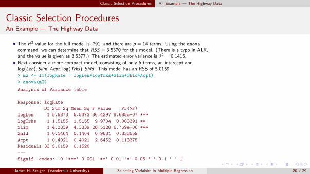
The R2 value for the full model is .791, and there are p = 14 terms. Using the anova

command, we can determine that RSS = 3.5370 for this model. (There is a typo in ALR,and the value is given as 3.5377.) The estimated error variance is σ2 = 0.1415.Next consider a more compact model, consisting of only 6 terms, an intercept andlog(Len),Slim,Acpt, log(Trks),Shld . This model has an RSS of 5.0159.

> m2 <- lm(logRate ~ logLen+logTrks+Slim+Shld+Acpt)

> anova(m2)

Analysis of Variance Table

Response: logRate

Df Sum Sq Mean Sq F value Pr(>F)

logLen 1 5.5373 5.5373 36.4297 8.685e-07 ***

logTrks 1 1.5155 1.5155 9.9704 0.003391 **

Slim 1 4.3339 4.3339 28.5128 6.769e-06 ***

Shld 1 0.1464 0.1464 0.9631 0.333559

Acpt 1 0.4021 0.4021 2.6452 0.113375

Residuals 33 5.0159 0.1520

---

Signif. codes: 0 '***' 0.001 '**' 0.01 '*' 0.05 '.' 0.1 ' ' 1




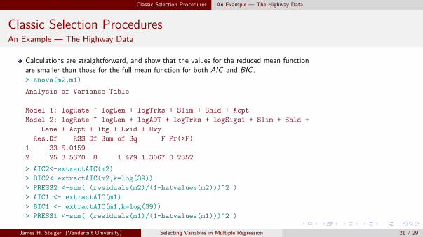
Calculations are straightforward, and show that the values for the reduced mean functionare smaller than those for the full mean function for both AIC and BIC .

> anova(m2,m1)

Analysis of Variance Table

Model 1: logRate ~ logLen + logTrks + Slim + Shld + Acpt

Model 2: logRate ~ logLen + logADT + logTrks + logSigs1 + Slim + Shld +

Lane + Acpt + Itg + Lwid + Hwy

Res.Df RSS Df Sum of Sq F Pr(>F)

1 33 5.0159

2 25 3.5370 8 1.479 1.3067 0.2852

> AIC2<-extractAIC(m2)

> BIC2<-extractAIC(m2,k=log(39))

> PRESS2 <-sum( (residuals(m2)/(1-hatvalues(m2)))^2 )

> AIC1 <- extractAIC(m1)

> BIC1 <- extractAIC(m1,k=log(39))

> PRESS1 <-sum( (residuals(m1)/(1-hatvalues(m1)))^2 )




> AIC1

[1] 14.00000 -65.61145

> AIC2

[1] 6.00000 -67.98662

> BIC1

[1] 14.00000 -42.32159

> BIC2

[1] 6.00000 -58.00525

> PRESS1

[1] 11.27222

> PRESS2

[1] 7.688042




The single most important tool in selecting a subset of variables is the analyst’sknowledge of the area under study and of each of the variables.In the highway accident data, Hwy is a factor, so all of its levels should probably either bein the candidate subset or excluded.Weisberg also makes the case that the variable log(Len) should be treated differentlyfrom the others, since its inclusion in the active predictors may be required by the wayhighway segments are defined.


Classic Selection Procedures Forward Selection

Classic Selection ProceduresForward Selection

In the preceding section, we simply compared two models.However, these two models represented only two of hundreds of possible models.Automated subset selection procedures can sort through many possible models andchoose one.Our first example of such an procedure is Forward Selection.In forward selection, we start with a base model and consider a set of additional possibleregressors. In what follows, assume that the base model is empty, i.e., has no regressors.

1 Consider all candidate subsets consisting of one term beyond the intercept, and find thesubset that minimizes the criterion of interest. If an information criterion is used, then thisamounts to finding the term that is most highly correlated with the response because itsinclusion in the subset gives the smallest residual sum of squares. Regardless of the criterion,this step requires examining k candidate subsets.

2 For all remaining steps, consider adding one term to the subset selected at the previous step.Using an information criterion, this will amount to adding the term with the largest partialcorrelation with the response given the terms already in the subset, and so this is a very easycalculation. Using cross-validation, this will require fitting all subsets consisting of the subsetselected at the previous step plus one additional term. At step j ,k − j + 1 subsets need to beconsidered.

3 Stop when all the terms are included in the subset, or when addition of another termincreases the value of the selection criterion.


Classic Selection Procedures Forward Selection

Classic Selection ProceduresForward Selection

If the number of terms beyond the intercept is k, this algorithm will consider at mostk + (k − 1) + . . .+ 1 = k(k − 1)/2 of the 2k possible subsets.For k = 10, the number of subsets actually considered is only 45 of the 1024 possiblesubsets. The subset among these 45 that has the best value of the criterion selected istentatively selected as the candidate.The algorithm requires modification if a group of terms is to be treated as all included orall not included, as would be the case with a factor.In such a case, we would have to consider adding the term or the group of terms thatproduces the best value on the criterion of interest.Each of the information criteria can now give different best choices because at each step,as we are no longer necessarily examining mean functions with pC fixed.


Classic Selection Procedures Backward Elimination

Classic Selection ProceduresBackward Elimination

Backward selection works in the reverse order. You start with a candidate subset and thendecide which terms can be eliminated.

1 Fit first with the full candidate subset.2 At the next step, consider all possible subsets obtained by removing one term other than

those to be forced to be in all mean functions from the candidate subset selected at the laststep. Using an information criterion, this amounts to removing the term with the smallestt-value in the regression summary because this will give the smallest increase in residual sumof squares. Using cross-validation, all subsets formed by deleting one term from the currentsubset must be considered.

3 Continue until all terms but those forced into all mean functions are deleted, or until the nextdeletion increases the value of the criterion.

Once again, we need consider only k(k − 1)/2 subsets. The subsets considered by forwardselection and backward elimination can be different.


Classic Selection Procedures Stepwise Regression

Classic Selection ProceduresStepwise Regression

The forward and backward algorithms can be combined into a stepwise method, where ateach step, a term is either deleted or added so that the resulting candidate mean functionminimizes the criterion function of interest. This will have the advantage of allowingconsideration of more subsets, without the need for examining all 2k subsets.

At each stage, the possibility is that a variable entered at a previous stage has nowbecome superfluous because of additional variables now in the model that were not in themodel when this variable was selected.To check on this, in the classic approach implemented in programs like SPSS, at eachstep a partial F test for each variable in the model is made as if it were the variableentered last. We look at the lowest of these F s and if the lowest one is sufficiently low(i.e., below the “F -to-remove” value, we remove the variable from the model, recomputeall the partial F s, and keep going until we can remove no more variables.


Computational Examples

Computational Examples

We illustrate forward selection with the Highway data.We start by defining some special variables and then defining, for convenience, ourmaximal model.

> Highway$sigs1 <- with(Highway, (sigs * len + 1)/len)

> f <- ~ log(len) + shld + log(adt) + log(trks) + lane + slim +lwid +

+ itg + log(sigs1) + acpt + htype

Next are the commands that set up a base model and start the Forward Selectionprocedure. They produce extensive output, so we’ll execute them in class and examinethe results there.

> m0 <- lm(log(rate) ~ log(len), Highway) # the base model

> m.forward <- step(m0, scope=f, direction="forward")

Here are the commands that produce Backwards Elimination.

> m1 <- update(m0, f)

> m.backward <- step(m1, scope = c(lower = ~ log(len)), direction="backward")

Here is the command for Stepwise Regression.

> m.stepup <- step(m0, scope=f)


Caution about Selection Methods

Caution about Selection Methods

It is easy to demonstrate that subset selection methods can overstate significance, andthat, after subset selection, the p-values printed in output are no longer valid.In some of my courses, we generate completely random data and then subject it toforward selection, finding a highly significant R2 when in fact the population squaredmultiple correlation is zero.Not only are p-values wrong, but of course the β values are badly biased too.Our online code file provides a demonstration, in which 99 completely random predictorsare assessed via Forward Selection.A number of “significant” regressors are found, and the R2 value of 0.3591 has a listedp-value of 0.0000174.What has gone wrong? (C.P.)


selecting variables in multiple regression - statpower notes/variableselection.pdf · selecting...

Documents