selecting the amount of smoothing in nonparametric regression estimation for complex surveys

This article was downloaded by: [Duke University Libraries]On: 10 October 2014, At: 21:23Publisher: Taylor & FrancisInforma Ltd Registered in England and Wales Registered Number: 1072954 Registeredoffice: Mortimer House, 37-41 Mortimer Street, London W1T 3JH, UK

Journal of Nonparametric StatisticsPublication details, including instructions for authors andsubscription information:http://www.tandfonline.com/loi/gnst20

Selecting the amount of smoothing innonparametric regression estimationfor complex surveysJ. D. Opsomer a & C. P. Miller aa Department of Statistics , Iowa State University , Ames, IA,50011, USAPublished online: 31 Jan 2007.

To cite this article: J. D. Opsomer & C. P. Miller (2005) Selecting the amount of smoothing innonparametric regression estimation for complex surveys, Journal of Nonparametric Statistics,17:5, 593-611, DOI: 10.1080/10485250500054642

To link to this article: http://dx.doi.org/10.1080/10485250500054642

PLEASE SCROLL DOWN FOR ARTICLE

Taylor & Francis makes every effort to ensure the accuracy of all the information (the“Content”) contained in the publications on our platform. However, Taylor & Francis,our agents, and our licensors make no representations or warranties whatsoever as tothe accuracy, completeness, or suitability for any purpose of the Content. Any opinionsand views expressed in this publication are the opinions and views of the authors,and are not the views of or endorsed by Taylor & Francis. The accuracy of the Contentshould not be relied upon and should be independently verified with primary sourcesof information. Taylor and Francis shall not be liable for any losses, actions, claims,proceedings, demands, costs, expenses, damages, and other liabilities whatsoeveror howsoever caused arising directly or indirectly in connection with, in relation to orarising out of the use of the Content.

This article may be used for research, teaching, and private study purposes. Anysubstantial or systematic reproduction, redistribution, reselling, loan, sub-licensing,systematic supply, or distribution in any form to anyone is expressly forbidden. Terms &Conditions of access and use can be found at http://www.tandfonline.com/page/terms-and-conditions

http://www.tandfonline.com/loi/gnst20

http://www.tandfonline.com/action/showCitFormats?doi=10.1080/10485250500054642

http://dx.doi.org/10.1080/10485250500054642

http://www.tandfonline.com/page/terms-and-conditions

http://www.tandfonline.com/page/terms-and-conditions

Nonparametric StatisticsVol. 17, No. 5, July 2005, 593–611

Selecting the amount of smoothing in nonparametricregression estimation for complex surveys

J. D. OPSOMER* and C. P. MILLER

Department of Statistics, Iowa State University, Ames, IA 50011, USA

(Received 30 December 2004; in final form 26 January 2005)

Model-assisted estimation is a common technique to improve the precision of finite population surveyestimators by taking advantage of relationships between the survey variables and the available auxiliaryinformation. Breidt and Opsomer introduced a nonparametric model-assisted estimator based on localpolynomial regression, which allows these relationships to be modeled nonparametrically. In thisarticle, we address the issue of how to select the amount of smoothing for the nonparametric regressioncomponent of the model-assisted estimator. The proposed smoothing parameter selection methodis based on minimizing a type of cross-validation criterion, suitably adjusted for the effect of thefinite population setting and the survey design. Asymptotic properties of the method are derived, andsimulation experiments show that it works well in practical settings as well.

Keywords: Model-assisted estimation; Local polynomial regression; Cross-validation

1. Introduction

The discipline of survey statistics is different from other areas of statistics in two impor-tant ways: the central role of the finite population and the reliance on a sampling design forinference. The goal of most survey techniques is to estimate descriptive characteristics for aparticular finite population of interest such as the mean or total of survey variables. For thispurpose, a sample of observations is selected according to a pre-specified sampling design,and an estimation approach that incorporates the design information is applied. Tradition-ally, inference for survey estimators has been design-based, which means that properties ofestimators are considered with respect to the probability distribution induced by repeated sam-pling according to the specified (and known) random sampling design [see ref. 1, for an earlyexample].

When an estimator uses only the design information in its construction, it is called purelydesign-based. This has the important advantage that its properties do not depend on any mod-eling assumptions about the finite population of interest, and in that sense, such an estimatorcan be considered ‘nonparametric’ (though that term is not typically used in this context).

*Corresponding author. Email: [email protected]

Nonparametric StatisticsISSN 1048-5252 print/ISSN 1029-0311 online © 2005 Taylor & Francis Group Ltd

http://www.tandf.co.uk/journalsDOI: 10.1080/10485250500054642

Dow

nloa

ded

by [

Duk

e U

nive

rsity

Lib

rari

es]

at 2

1:23

10

Oct

ober

201

4

594 J. D. Opsomer and C. P. Miller

The drawback of purely design-based estimators is that they can be inefficient, especially insurveys of moderate size.

In many surveys, auxiliary information is readily available for the population and can beused to improve the precision of design-based estimators. Ratio and regression estimators[e.g., ref. 2] have a long history of use in survey estimation. Generalized regression estimationand, more generally, model-assisted estimation [3] provide a framework for incorporatingsuperpopulation models into design-based estimation (in the survey context, models for thepopulation are referred to as superpopulation models, and we will use the same terminol-ogy here). Model-assisted estimators are constructed in such a way that the superpopulationmodel assumptions improve the precision of the estimators when the model is true, but thedesign-based properties of the estimator remain valid even when the modeling assumptionsare violated.

Traditionally, model-assisted estimation has relied on parametric, most often linear, models.Recently, Wu and Sitter [4] introduced a nonlinear version of model-assisted estimation,which can be useful if the linear model is not appropriate. When those linear or nonlinearmodels are correct for the sampled population, regression estimators that take advantage ofthe superpopulation model are more efficient [i.e., have a smaller design mean squared error(MSE)] than estimators that ignore it, or than those that use an incorrectly specified model.As the superpopulation model is typically unknown, there is an incentive to use models thatare not too restrictive.

Breidt and Opsomer [5] proposed a type of model-assisted estimator that relies on a non-parametric superpopulation model and used local polynomial regression [e.g., ref. 6] as thefitting method for the superpopulation model. By relaxing the assumptions on the functionalform of the superpopulation model, this nonparametric approach makes it possible to improvethe design efficiency of regression estimators in the case where the true relationship betweenthe variable of interest and the auxiliary variable is difficult to specify a priori. Breidt andOpsomer [5] proved that the local polynomial regression estimator shares the good designproperties of the traditional regression estimators, including design consistency, asymptoticnormality, and calibration.

As in any nonparametric regression method, the practical properties of the estimator dependon the choice of a smoothness tuning parameter, i.e., the bandwidth in local polynomialregression. In Breidt and Opsomer [5], the bandwidth was treated as a fixed quantity and theissue of how to best select a bandwidth value was not addressed. In this article, we will explorethe issue of smoothing parameter selection for nonparametric model-assisted estimation andpropose a sample-based criterion that can be used for this purpose.

Selecting an appropriate value for the bandwidth in the survey estimation context is quitedifferent from doing so in traditional nonparametric regression. The criterion for optimalbandwidth choice, in this case the design-based MSE of the estimator, measures deviationsbetween a sample-based estimator and a finite population quantity, not deviations betweenan estimator and a model. In particular, this implies that the criterion does not depend onthe unknown smooth model function directly, but only through a population-based fit to thatfunction. Hence, traditional model-based intuition about bias and variance relative to thatunknown model function do not apply. This will be further explored in following sections.

Another important difference between the current criterion and traditional ones, such ascross-validation (CV), is that it depends on the nonparametric estimator (and hence the band-width) in an unconventional and complicated way, because it needs to incorporate the samplingdesign. Stratification, unequal probability sampling, and clustering all have an impact on theestimation procedure and need to be accounted for in bandwidth selection.

Because of the unique nature of the survey-appropriate criterion and the need to incor-porate the sampling design, existing selection methods such as (generalized) CV or the

Dow

nloa

ded

by [

Duk

e U

nive

rsity

Lib

rari

es]

at 2

1:23

10

Oct

ober

201

4

Smoothing regression for complex surveys 595

information-based approach of Hurvich et al. [7] cannot be applied in this case and needto be replaced by a method targeted specifically for the model-assisted estimator. To date, nosuch method is available, and as will be discussed further in subsequent sections, the common-sense approach of minimizing a sample-based estimator of the design MSE will actually leadto the wrong choice of bandwidth.

We will address two issues related to the choice of bandwidth in nonparametric regressionestimation. First, we will show that the asymptotic design properties of the local polynomialregression estimator proven in Breidt and Opsomer [5] continue to hold when the bandwidthis allowed to vary over a range of values, providing an additional amount of robustness fortheir results. Second, we will propose a sample-driven method for selecting an appropriatebandwidth for model-assisted estimation based on a CV adjustment to the estimated MSE.In particular, we will show that this ‘cross-validated bandwidth’ is a good estimator for thebandwidth that minimizes the design MSE of the model-assisted estimator, both theoreticallyand through simulation experiments. The proposed method is also quite straightforward toimplement in practice and can be generalized to more complicated nonparametric and semi-parametric models. As in Breidt and Opsomer [5], we will restrict attention in this article to thesituation where the auxiliary variable is one-dimensional and continuous. Developing a moregeneral framework would certainly be valuable but significantly complicate the theoreticalportions of the article.

The rest of the paper is organized as follows. Section 2 defines the estimator and thebandwidth selection method. The main theoretical results are in section 3. In section 4, wepresent simulation results illustrating how the CV-based criterion works in practice.

2. Definition of estimator and bandwidth selection

2.1 Model-assisted local polynomial regression estimator

Suppose that two continuous variables x and y are defined for elements of a finite populationU of size N , with the values of x known for all the elements of U , but those for y only availableafter taking a sample s ⊂ U . In the finite population context, suppose that we are interestedin estimating the finite population quantity ty = ∑

U yi , the total of y for all elements in thepopulation, based on {yi, i ∈ s}. The sample s of size n is selected randomly on the basis ofthe known sampling design p(·) with associated inclusion probabilities πi = Pr(i ∈ s) andπij = Pr(i, j ∈ s) for i, j ∈ U . The purely design-based Horvitz–Thompson (HT) estimatorof ty ,

tyπ =∑i∈s

yi

πi

(1)

[8], is unbiased with respect to the sampling design p(·), and its design variance is given by

Varp(tyπ ) =∑i,j∈U

(πij − πiπj )yi

πi

yj

πj

. (2)

Model-assisted estimation attempts to improve on the precision with which ty is estimated byusing auxiliary information available for the population (the variable x in this case).

Suppose now that x and y are related, but that the exact form of that relationship is unknown.It seems reasonable to assume that if we could estimate that relationship, then that estimatedrelationship could be used to create a more accurate estimator of ty than equation (1). Theadvantage of using nonparametric regression in this context is that it is possible to estimate the

Dow

nloa

ded

by [

Duk

e U

nive

rsity

Lib

rari

es]

at 2

1:23

10

Oct

ober

201

4


relationship between both variables without having to specify its exact form, requiring onlythat it be continuous and smooth.

We briefly review the nonparametric model-assisted estimator of Breidt and Opsomer [5].The estimator is based on the following assumed superpopulation model:

yi = m(xi) + εi, (3)

for i ∈ U , where m(·) is an unknown smooth function and the {εi} are independent and followa distribution F with mean 0 and variance v(xi). Let q be the degree of the regression, K thekernel function. Define the N × (q + 1) matrix

XUi :=1 x1 − xi · · · (x1 − xi)

q

......

. . ....

1 xN − xi · · · (xN − xi)q

.

Assume for now that bandwidth h has been chosen for population U . Define the N × N matrixWUi to be diagonal, with j th diagonal element equal to (1/h)K(xj − xi/h). Let yU be thevector of y-values for U . Let e1 be a vector with 1 in position 1 and 0 in all other positions.The local polynomial estimator for m(xi) that uses data for the entire population is

mi := eT1 (XT

UiWUiXUi)−1XT

UiWUiyU

= wTUiyU .

This is the ‘classical’ local polynomial regression estimator of m(xi) [see, e.g., ref. 6]. If allmi , i ∈ U were known, we could construct the difference estimator of ty ,

t∗y =∑i∈s

yi − mi

πi

+∑i∈U

mi

[ref. 3, p. 221]. This estimator is design unbiased and its design variance is given by

Varp(t∗y ) =∑i,j∈U

(πij − πiπj )yi − mi

πi

yj − mj

πj

. (4)

By comparing the variances in equations (2) and (4), it is clear that, when the superpopulationmodel is appropriate for the data, the difference estimator will have a smaller variance thanthe HT estimator: the former depends on the population residuals yi − mi , whereas the latterdepends on the yi themselves.

The estimator t∗y is unfeasible, because the y-values are known only for sample elements sothat the mi cannot be computed. However, the ‘population fits’ mi can be estimated from thesample, so that we can construct a sample-based approximation to t∗y as follows. For i ∈ U ,let Xsi be the n × (q + 1) matrix whose rows are of form

[1 xj − xi · · · (xj − xi)q],

for all j ∈ s. Define Wsi to be the n × n diagonal matrix whose diagonal elements are equalto (1/πjh)K(xj − xi/h), j ∈ s. Finally, choose a constant ν > 0. Let ys be the vector ofy-values associated with elements of s. A sample-based local polynomial estimator for mi is

mi := eT1

(XT

siWsiXsi + ν

Nq+1I)−1

XTsiWsiys

= wTsiys . (5)

Dow

nloa

ded

by [

Duk

e U

nive

rsity

Lib

rari

es]

at 2

1:23

10

Oct

ober

201

4


The estimator mi is a local polynomial estimator, but the inclusion of the sampling weights inWsi makes it a design-based estimator for the population fit mi . The addition of (ν/Nq+1)Iin wsi ensures that the matrix to be inverted has eigenvalues bounded below by ν/Nq+1, sothat mi is always well-defined, even if the matrix XT

siWsiXsi is singular. This adjustment issimilar to the ridging approach recommended by Seifert and Gasser [9] for local polynomialregression when the xi are random, which is the case in the sample s. We did not attempt toselect the value for the ridging parameter adaptively, as the focus on the current paper wason the selection of the bandwidth parameter h. In section 4, we evaluate the effect of settingν = 0 vs. ν > 0 in simulations.

The model-assisted local polynomial regression estimator for ty is defined as

ty :=∑i∈s

yi − mi

πi

+∑i∈U

mi . (6)

The properties of ty are studied in Breidt and Opsomer [5] for the case where h is fixed.Under an appropriate set of assumptions on the population and the sampling design, ty isasymptotically equivalent to t∗y and will share its asymptotic properties.

2.2 Bandwidth selection

As shown in Breidt and Opsomer [5], Varp(t∗y ) in equation (4) is an asymptotic approximationto MSEp(ty) and the MSE of ty , and both are consistently estimated by

V (ty) :=∑i,j∈s

πij − πiπj

πij

yi − mi

πi

yj − mj

πj

. (7)

In model-assisted estimation of a population total, the design bias is asymptotically negligiblerelative to the design variance, so that the estimator (7) indeed estimates the leading termin MSEp(ty). The conditions on the bandwidth sufficient for this to hold are that h → 0 andnh2 → ∞ [see ref. 5], implying that the traditional bias-variance trade-off observed in model-based nonparametric estimation of an unknown regression function does apply here. Speakingsomewhat loosely, this can be explained by the fact that the leading term of MSEp(ty) dependsonly on the residuals yi − mi (which are almost completely dominated by noise), whereasthe MSE of the model-based nonparametric regression estimator depends on the deviationsmi − m(xi) (which are subject to both estimation bias and variance).

The estimator (6) depends on the value chosen for the bandwidth h, so that its MSE can beviewed as a function of h. We would like to select (or, more acurately, estimate) the bandwidthvalue that minimizes MSEp(ty). Let hopt denote this optimal bandwidth, which is unknown.As V (ty) is design consistent for MSEp(ty), it might seem tempting to try to estimate hopt bythe value of h that minimizes V (ty). It turns out that this is not a valid estimator in practice,as the following heuristic reasoning illustrates. For any i ∈ s, yi is a summand of mi and mi

can be made to be close to yi by letting h → 0, only subject to maintaining the existence ofmi . Hence, V (ty) can be made arbitrarily small by letting h approach 0. On the other hand,MSEp(ty) remains in general (much) larger than 0 for all values of h. Hence, the minimizerof V (ty) is a poor choice as an estimator of hopt. The simulations discussed in section 4subsequently also confirm that in practice, V (ty) is unsuitable to use as bandwidth selectioncriterion.

We can modify V (ty) so that it provides a more suitable criterion for sample-driven band-width selection, using ideas of CV for linear smoothers [see, e.g., ref. 10, p. 46]. Specifically,

Dow

nloa

ded

by [

Duk

e U

nive

rsity

Lib

rari

es]

at 2

1:23

10

Oct

ober

201

4


we replace each estimator mi in equation (7) by the ‘leave-one-out’ estimator m(−)i . To do this,

we replace wsi in equation (5) by a modified smoothing vector w′si with elements

w′sij =

wsij

1 − wsii

if j �= i

0 if i = j,(8)

where wsij denotes the j th element of the vector wsi , and set m(−)i := ∑

j∈s w′sij yi . Intuitively,

it should be clear that this will avoid the problem described earlier for mi , since we onlyuse {yj : j �= i, i ∈ s} to estimate m

(−)i , so that letting the bandwidth h go to 0 no longer

automatically results in m(−)i approaching yi . The modification of V (ty) we propose to use as

a bandwidth selection criterion is defined as

VCV(h) :=∑i,j∈s

πij − πiπj

πij

yi − m(−)i

πi

yj − m(−)j

πj

. (9)

We will refer to VCV(h) as the design-based CV criterion, from its similarity with the model-based CV criterion used for bandwidth selection in function estimation [see, ref. 10, p. 46].Note, however, that it fully reflects the sampling design, both in the construction of the varianceestimator and in the estimation of the mi . We will write hCV for the minimizer of VCV(h), anduse it as an estimator of hopt, the minimizer of MSEp(ty).As is the case for the model-based CVcriterion, the relationship between the leave-one-out weights and the original weights givenin equation (8) implies that the computation of the leave-one-out fit m

(−)i does not require that

the local polynomial regression operation be repeated for each i. Hence, the VCV(h) is readilycomputed based on the original smoothing weights wsi .

3. Theoretical properties

We begin by describing the design-based asymptotic framework in which we will deriveour results. In the survey context, asymptotic analysis requires the finite population to beembedded in a sequence of populations generated from a superpopulation, and the samples tobe drawn according to a sequence of sampling designs corresponding to this finite populationsequence. Specifically, we assume an increasing sequence of populations UN indexed by N ,with #{UN+1} ≥ #{UN }. For each N , a sample sN of size nN is selected from UN according toa sampling design pN(·). The sample size nN may be fixed (as is the case for simple randomsampling) or random (as in the case of Bernoulli sampling); we do not specify the exactsampling scheme. This increasing population framework is the same as that used in Breidtand Opsomer [5] and is based on that of Isaki and Fuller [11].

For each sN , we regress with a bandwidth h chosen from an interval HN , where HN is aninterval bounded away from 0 and further specified subsequently. With each i ∈ UN , we asso-ciate xi , yi ∈ R. Formally, we will treat x as a random variable with probability density f (·).For each N , {xi : i ∈ UN } are independent, and the yi follow model (3). We are allowing theinclusion probabilities πi to depend on the values of the auxiliary variable xi , as would happenin probability-proportional-to-size sampling designs, for instance. The theoretical results areprovided in three theorems, which rely on several sets of assumptions. The assumptions tendto be fairly technical; they have therefore been placed in Appendix A.1. Outlines of proofs forthe three theorems are given in Appendix A.2, and a set of accompanying technical lemmasare given without proof in Appendix A.3. Additional technical details can be found in Millerand Opsomer [12].

Dow

nloa

ded

by [

Duk

e U

nive

rsity

Lib

rari

es]

at 2

1:23

10

Oct

ober

201

4


The first theorem proves uniform almost sure convergence of the local polynomial regressionestimator ty . It also implies that the estimator ty is an asymptotically unbiased estimator andconsistent of ty , for any sequence of bandwidths h in an interval HN .

THEOREM 1 Assume conditions POP-1 to POP-4, SD-1 to SD-3, EST-1 to EST-4, and INT-2in Appendix A.1. Also assume INT-1 holds for t = 1, 2. Then with probability one, over allsequences of samples {sN }N≥1, auxiliary populations {{xj }j∈UN

}N≥1, and error populations{{εj }j∈UN

}N≥1,

limN→∞ sup

h∈HN

∣∣∣∣ ty − ty

N

∣∣∣∣ = 0.

Theorem 1 is similar to Theorem 1 in ref. [5] but extends it in two directions. First, itshows that their result does not depend on any specific bandwidth, but rather, it holds uni-formly for any bandwidth in HN . Second, it shows that the consistency of the estimator tyis with probability one over all samples and all populations. While this is not, strictly speak-ing, a purely design-based result as written, it implies design consistency as well as modelconsistency.

The assumptions on which this theorem is based (see Appendix) may seem elabo-rate, but they allow great freedom in choosing the kernel and bandwidth. In particular, if∫ |u|�Kj (u) du < ∞ for large � and j , then we can set HN = (CaN

−a, CbN−b), where a can

be very close to 1/2 and b can be very close to 0. Hence, the bandwidth set over which we areallowing h to vary is very wide and includes the rates normally considered ‘optimal’ in theclassical nonparametric regression context (for instance, O(n1/5) for local linear regression).Restricting the bandwidth to a certain range of rates is commonly done in proving results forbandwidth selectors [see, for instance, ref. 13 for a condition similar to ours]. The range weconsider excludes the case h → ∞, which would be the correct choice when m(·) is exactlyequal to a polynomial of degree ≤q. This restriction was required to make the theoreticalderivations more tractable. In the simulations in section 4, we will therefore also considercases that could lead to bandwidths outside of those bounds and argue that the proposedmethod still leads to reasonable bandwidths in those cases.

Most commonly used kernels satisfy the conditions specified by our assumptions, for allpositive j and �. Among these are the biweight, triangular, Epanechnikov, Gaussian, anduniform kernels.

The following theorem shows that the approximation of the design MSE of ty by Varp(t∗y )

in equation (4), as done in Theorem 2 of ref. [5], holds uniformly for bandwidths in HN . Inother words, the difference estimator variance in equation (4) is consistent for the design MSEof the local polynomial regression estimator ty , not only for a fixed sequence of bandwidthhN but also for any sequence of bandwidths h in HN .

THEOREM 2 Assume conditions POP-1 to POP-5, SD-1 to SD-3, EST-1 to EST-4, and INT-2,INT-3, and INT-1 with t = 1, 2 in Appendix A.1. Then, with probability one, the auxiliarypopulations {{xj }j∈UN

}N≥1 and error populations {{εj }j∈UN}N≥1 are such that

limN→∞ sup

h∈HN

1

N

∣∣∣∣∣∣MSEp(ty) −∑

i,j∈UN


πi

yj − mj

πj

∣∣∣∣∣∣ = 0.

For the next theorem, we write MSEp(h) for the MSE of ty as a function of the bandwidthh, and hopt = arg minh∈HN

MSEp(h).

Dow

nloa

ded

by [

Duk

e U

nive

rsity

Lib

rari

es]

at 2

1:23

10

Oct

ober

201

4


THEOREM 3 Let all conditions in Appendix A.1 hold. Assume INT-1 holds for t ∈ {1, 2, 4}.Then with probability one, the auxiliary populations {{xj }j∈UN

}N≥1, error populations{{εj }j∈UN

}N≥1, and samples {sN }N≥1 are such that

limN→∞ sup

h∈HN

|VCV(h) − MSEp(h)|MSEp(hopt)

= 0.

This theorem shows that the difference between the functions VCV(h) and MSEp(h) goes to0 asymptotically, whatever bandwidth we choose in HN . Hence, VCV(h) is an asymptoticallyequivalent criterion to MSEp(h) for selecting a bandwidth.

In section 4, we will evaluate how well this asymptotic result translates to the finite sampleperformance of VCV(h) as a design-based bandwidth selection criterion.

4. Simulations

As we are evaluating the design-based properties of the bandwidth selection method, wegenerate a single finite population and draw repeated samples from it. Specifically, a randompopulation of N = 1000 values of x is generated from the uniform distribution on [0, 1], and1000 values for the errors ε were drawn from N(0, 1). This one error population was used forall simulations, up to multiplication by σ . Eight populations of y were generated as follows:

yi� = m�(xi) + εi 1 ≤ i ≤ 1000, 1 ≤ � ≤ 8

where {m�}8�=1 are predefined functions given in the first two columns of table 1. The finite

population quantities of interest are ty = ∑1000i=1 yil for each l.

The samples are drawn by simple random sampling without replacement. For each simu-lation run, M = 1000 samples are drawn from {(xi, yi)}. For each sample, we compute theestimator ty in equation (6) for hopt and hCV. The optimal bandwidths hopt for each y-populationare not sample-based, but since they do not have an explicit expression, they are computed byminimizing a simulation-based approximation to the function MSEp(h). This function is con-structed by simulating repeated samples from these populations for a grid of bandwidths overthe interval [0.01, 1], and finding the functions MSEp(h) by averaging over these simulations,followed by interpolation.

For each sample, the bandwidth hCV is sought through a search algorithm implemented inMatlab 6.5.1, which uses expression (9). A simulation run is determined by sample size n,

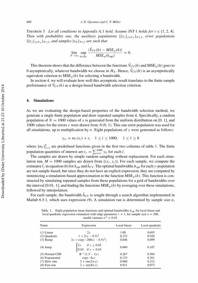
Table 1. Eight population mean functions and optimal bandwidths hopt for local linear andlocal quadratic regression estimation with ridge parameter ν = 1, for sample size n = 200,

model variance σ 2 = 0.01.

Name Expression Local linear Local quadratic

(1) Linear 2x 1.00 0.693(2) Quadratic 1 + 2(x − 0.5)2 0.232 0.920(3) Bump 2x + exp(−200(x − 0.5)2) 0.046 0.099

(4) Jump

{2x if x ≤ 0.650.65 if x > 0.65

0.060 0.107

(5) Normal CDF �−1(1.5 − 2x) 0.267 0.504(6) Exponential exp(−8x) 0.123 0.361(7) Slow sine 2 + sin(2πx) 0.060 0.212(8) Fast sine 2 + sin(8πx) 0.031 0.073

Dow

nloa

ded

by [

Duk

e U

nive

rsity

Lib

rari

es]

at 2

1:23

10

Oct

ober

201

4


error variance σ 2, degree of local regression q, and ridge constant ν. Simulations are done forn ∈ {100, 200, 500}, σ 2 ∈ {0.01, 0.16}, q ∈ {1, 2}, and ν = 1. Simulations are also done withn = 200, σ 2 ∈ {0.01, 0.16}, q ∈ {1, 2}, and ν = 0 (no ridge adjustment). The major findingsof those simulations are reported subsequently.

The last two columns of table 1 show the optimal bandwidths hopt for both local linear andlocal quadratic regression for a typical simulation run (ν = 1, n = 200, and σ 2 = 0.01 in thiscase). Clearly, hopt varies widely across functions and also between the two nonparametricmethods, with local quadratic regression typically requiring larger bandwidths. Another pointof note in table 1 is that, in the cases where the true mean function corresponds exactly to thepolynomial used in the nonparametric regression, the optimal bandwidth becomes very large.This corresponds to the cases with linear mean for the local linear regression, and those withlinear or quadratic mean for the local quadratic regression. In those cases, the local polynomialmethod could be replaced by an equivalent global polynomial method, because the polynomialmodel is correctly specified, and that is indeed what the large optimal bandwidth is attemptingto achieve. Note that these cases are those for which the theory of section 3 does not hold,since the bandwidth range we considered requires the bandwidth to decrease at a rate that isat least n−1/2.

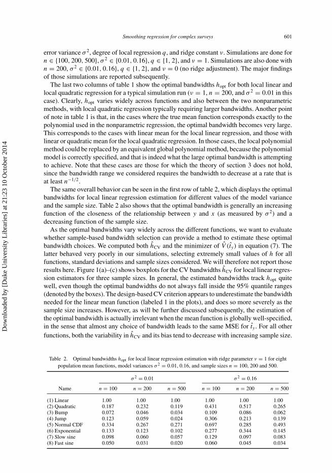
The same overall behavior can be seen in the first row of table 2, which displays the optimalbandwidths for local linear regression estimation for different values of the model varianceand the sample size. Table 2 also shows that the optimal bandwidth is generally an increasingfunction of the closeness of the relationship between y and x (as measured by σ 2) and adecreasing function of the sample size.

As the optimal bandwidths vary widely across the different functions, we want to evaluatewhether sample-based bandwidth selection can provide a method to estimate these optimalbandwidth choices. We computed both hCV and the minimizer of V (ty) in equation (7). Thelatter behaved very poorly in our simulations, selecting extremely small values of h for allfunctions, standard deviations and sample sizes considered. We will therefore not report thoseresults here. Figure 1(a)–(c) shows boxplots for the CV bandwidths hCV for local linear regres-sion estimators for three sample sizes. In general, the estimated bandwidths track hopt quitewell, even though the optimal bandwidths do not always fall inside the 95% quantile ranges(denoted by the boxes). The design-based CV criterion appears to underestimate the bandwidthneeded for the linear mean function (labeled 1 in the plots), and does so more severely as thesample size increases. However, as will be further discussed subsequently, the estimation ofthe optimal bandwidth is actually irrelevant when the mean function is globally well-specified,in the sense that almost any choice of bandwidth leads to the same MSE for ty . For all otherfunctions, both the variability in hCV and its bias tend to decrease with increasing sample size.

Table 2. Optimal bandwidths hopt for local linear regression estimation with ridge parameter ν = 1 for eightpopulation mean functions, model variances σ 2 = 0.01, 0.16, and sample sizes n = 100, 200 and 500.

σ 2 = 0.01 σ 2 = 0.16

Name n = 100 n = 200 n = 500 n = 100 n = 200 n = 500

(1) Linear 1.00 1.00 1.00 1.00 1.00 1.00(2) Quadratic 0.187 0.232 0.119 0.431 0.517 0.265(3) Bump 0.072 0.046 0.034 0.109 0.086 0.062(4) Jump 0.123 0.059 0.024 0.306 0.213 0.139(5) Normal CDF 0.334 0.267 0.271 0.697 0.285 0.493(6) Exponential 0.133 0.123 0.102 0.277 0.344 0.145(7) Slow sine 0.098 0.060 0.057 0.129 0.097 0.083(8) Fast sine 0.050 0.031 0.020 0.060 0.045 0.034

Dow

nloa

ded

by [

Duk

e U

nive

rsity

Lib

rari

es]

at 2

1:23

10

Oct

ober

201

4


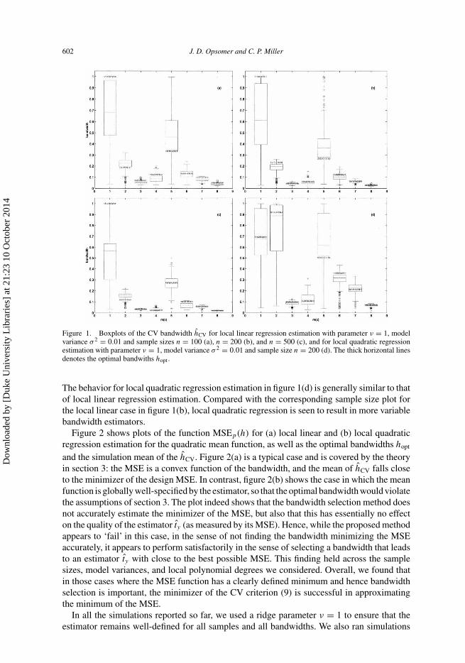
Figure 1. Boxplots of the CV bandwidth hCV for local linear regression estimation with parameter ν = 1, modelvariance σ 2 = 0.01 and sample sizes n = 100 (a), n = 200 (b), and n = 500 (c), and for local quadratic regressionestimation with parameter ν = 1, model variance σ 2 = 0.01 and sample size n = 200 (d). The thick horizontal linesdenotes the optimal bandwiths hopt .

The behavior for local quadratic regression estimation in figure 1(d) is generally similar to thatof local linear regression estimation. Compared with the corresponding sample size plot forthe local linear case in figure 1(b), local quadratic regression is seen to result in more variablebandwidth estimators.

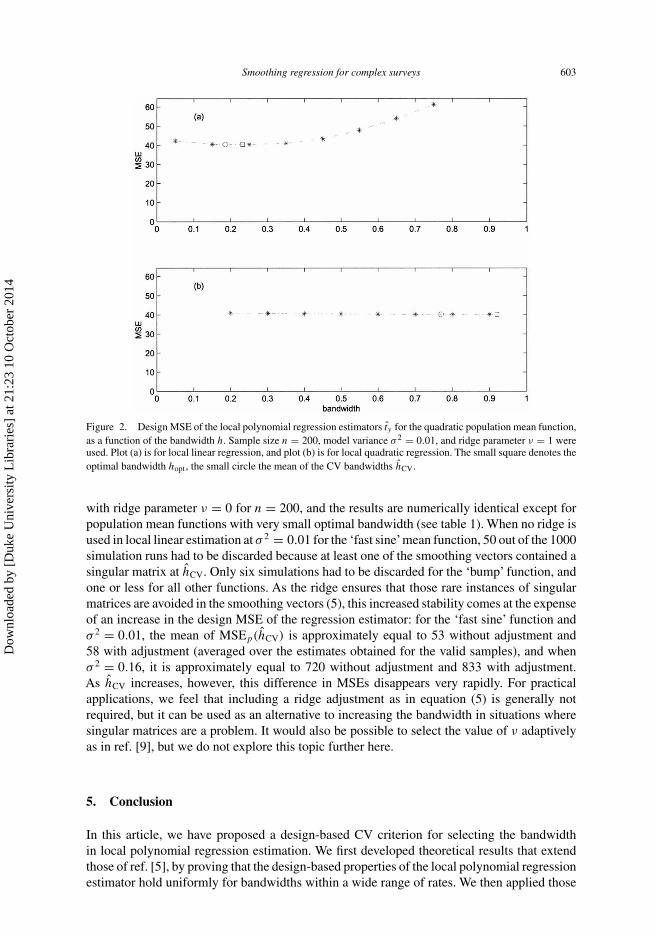
Figure 2 shows plots of the function MSEp(h) for (a) local linear and (b) local quadraticregression estimation for the quadratic mean function, as well as the optimal bandwidths hopt

and the simulation mean of the hCV. Figure 2(a) is a typical case and is covered by the theoryin section 3: the MSE is a convex function of the bandwidth, and the mean of hCV falls closeto the minimizer of the design MSE. In contrast, figure 2(b) shows the case in which the meanfunction is globally well-specified by the estimator, so that the optimal bandwidth would violatethe assumptions of section 3. The plot indeed shows that the bandwidth selection method doesnot accurately estimate the minimizer of the MSE, but also that this has essentially no effecton the quality of the estimator ty (as measured by its MSE). Hence, while the proposed methodappears to ‘fail’ in this case, in the sense of not finding the bandwidth minimizing the MSEaccurately, it appears to perform satisfactorily in the sense of selecting a bandwidth that leadsto an estimator ty with close to the best possible MSE. This finding held across the samplesizes, model variances, and local polynomial degrees we considered. Overall, we found thatin those cases where the MSE function has a clearly defined minimum and hence bandwidthselection is important, the minimizer of the CV criterion (9) is successful in approximatingthe minimum of the MSE.

In all the simulations reported so far, we used a ridge parameter ν = 1 to ensure that theestimator remains well-defined for all samples and all bandwidths. We also ran simulations

Dow

nloa

ded

by [

Duk

e U

nive

rsity

Lib

rari

es]

at 2

1:23

10

Oct

ober

201

4


Figure 2. Design MSE of the local polynomial regression estimators ty for the quadratic population mean function,as a function of the bandwidth h. Sample size n = 200, model variance σ 2 = 0.01, and ridge parameter ν = 1 wereused. Plot (a) is for local linear regression, and plot (b) is for local quadratic regression. The small square denotes theoptimal bandwidth hopt , the small circle the mean of the CV bandwidths hCV.

with ridge parameter ν = 0 for n = 200, and the results are numerically identical except forpopulation mean functions with very small optimal bandwidth (see table 1). When no ridge isused in local linear estimation at σ 2 = 0.01 for the ‘fast sine’mean function, 50 out of the 1000simulation runs had to be discarded because at least one of the smoothing vectors contained asingular matrix at hCV. Only six simulations had to be discarded for the ‘bump’ function, andone or less for all other functions. As the ridge ensures that those rare instances of singularmatrices are avoided in the smoothing vectors (5), this increased stability comes at the expenseof an increase in the design MSE of the regression estimator: for the ‘fast sine’ function andσ 2 = 0.01, the mean of MSEp(hCV) is approximately equal to 53 without adjustment and58 with adjustment (averaged over the estimates obtained for the valid samples), and whenσ 2 = 0.16, it is approximately equal to 720 without adjustment and 833 with adjustment.As hCV increases, however, this difference in MSEs disappears very rapidly. For practicalapplications, we feel that including a ridge adjustment as in equation (5) is generally notrequired, but it can be used as an alternative to increasing the bandwidth in situations wheresingular matrices are a problem. It would also be possible to select the value of ν adaptivelyas in ref. [9], but we do not explore this topic further here.

5. Conclusion

In this article, we have proposed a design-based CV criterion for selecting the bandwidthin local polynomial regression estimation. We first developed theoretical results that extendthose of ref. [5], by proving that the design-based properties of the local polynomial regressionestimator hold uniformly for bandwidths within a wide range of rates. We then applied those

Dow

nloa

ded

by [

Duk

e U

nive

rsity

Lib

rari

es]

at 2

1:23

10

Oct

ober

201

4


results to show that the proposed bandwidth selection criterion is asymptotically equivalentto minimizing the design MSE of the estimator. A simulation study was used to show that theestimated bandwidth generally tracks the optimal bandwidth quite well.

The CV approach proposed here extends readily to the selection of the amount of smooth-ing for other nonparametric model-assisted estimation contexts, for instance when the localpolynomial regression is replaced by a spline-based method or a multivariate method such asgeneralized additive models is used. In the latter case, multiple smoothing parameters mighthave to be selected for different covariates. Although the theoretical portion of this article doesnot apply directly to those contexts, the practical advantages of CV as a correction foroverfitting in model selection are known to hold across a wide range of parametric and non-parametric modeling situations. Hence, until alternative methods are developed for smoothingparameter selection in the finite population estimation context, we recommend using thedesign-based CV criterion proposed here whenever data-driven smoothing parameter selectionfor survey estimation is required.

References

[1] Neyman, J., 1934, On the two different aspects of the representative method: the method of stratified samplingand the method of purposive selection. Journal of the Royal Statistical Society, 97, 558–606.

[2] Cochran, W.G., 1977, Sampling Techniques (3rd edn) (New York: John Wiley & Sons).[3] Särndal, C.-E., Swensson, B. and Wretman, J., 1992, Model Assisted Survey Sampling (New York: Springer-

Verlag).[4] Wu, C. and Sitter, R.R., 2001, A model-calibration approach to using complete auxiliary information from

survey data. Journal of the American Statistical Association, 96, 185–193.[5] Breidt, F.J. and Opsomer, J.D., 2000, Local polynomial regression estimators in survey sampling. Annals of

Statistics, 28, 1026–1053.[6] Wand, M.P. and Jones, M.C., 1995, Kernel Smoothing (London: Chapman and Hall).[7] Hurvich, C., Simonoff, J. and Tsai, C.-L., 1998, Smoothing parameter selection in nonparametric regression

using an improved Akaike Information Criterion. Journal of the Royal Statistical Society, Series B, 60, 271–293.[8] Horvitz, D.G. and Thompson, D.J., 1952, A generalization of sampling without replacement from a finite

universe. Journal of the American Statistical Association, 47, 663–685.[9] Seifert, B. and Gasser, T., 2000, Data adaptive ridging in local polynomial regression. Journal of Computational

and Graphical Statistics, 9, 338–360.[10] Hastie, T.J. and Tibshirani, R.J., 1990, Generalized Additive Models (Washington, DC: Chapman and Hall).[11] Isaki, C. and Fuller, W., 1982, Survey design under the regression superpopulation model. Journal of the

American Statistical Association, 77, 89–96.[12] Miller, C.P. and Opsomer, J.D., 2004, Theorems on bandwidth selection for local polynomial regression with

survey data. Department of Statistics, Iowa State University, Preprint 04–18.[13] Härdle,W. and Marron, J.S., 1985, Optimal bandwidth selection in nonparametric regression function estimation.

Annals of Statistics, 13, 1465–1481.

Technical Appendix A

A.1 Assumptions

A.1.1. Assumptions on population

POP-1 Distribution of x: {xi : i ∈ UN } are independent and identically distributed, with den-sity f . Support (f ) = [L, U ]; f is continuous and bounded away from 0 on (L, U).(Equivalently, the assumption of regular and equally spaced xi can be used; see ref.[12] for details).

POP-2 Errors: {εi}i∈UNare independent for all N .

POP-3 Condition on variance function v(x): ∃c1, c2 > 0 such that v(x) ∈ (c1, c2), ∀x ∈[L, U ].

Dow

nloa

ded

by [

Duk

e U

nive

rsity

Lib

rari

es]

at 2

1:23

10

Oct

ober

201

4


POP-4 Conditions on mean function m(x): m(x) is Lipschitz continuous of order lm on [L, U ].That is, ∃lm > 0, Cm > 0 such that if x and y are in [L, U ], then |m(x) − m(y)| <

Cm|x − y|l(m) . We further assume that lm > 0.5.POP-5 f is Lipschitz continuous. That is, ∃lf > 0, Cf > 0 such that x, y ∈ [L, U ] ⇒

|f (x) − f (y)| < Cf |x − y|l(f ) .

A.1.2 Assumptions on sampling design

SD-1 Condition on sample size: ∃τ > 0 such that with probability one,

limM→∞ inf

N>M

nN

N> τ.

SD-2 Bounds on first and second order inclusion probabilities: ∃λ, λ∗ > 0 such that withprobability one, πj > λ and πij > λ∗, ∀i, j ∈ UN , N ≥ 1.

SD-3 Dependency between xi and πi : for a sample sN that contains j , define x(sN/{j}) :={xi : i ∈ sN , i �= j}, and for a measurable subset R ⊂ R, let

WR := #{j ∈ UN :xj ∈ R}N

pm(R) := min

{Pr

(xj ∈ R|sN , x

(sN

{j}))}

pM(R) := max

{Pr

(xj ∈ R|sN , x

(sN

{j}))}

where the extrema are over all j ∈ UN , all samples sN that contain j , and all assignments{xi : i ∈ sN/{j}}. Assume that ∃C1, C2 > 0 such that for any measurable R ⊂ [L, U ],

C1WR < pm(R) < pM(R) < C2WR.

(This assumption puts a limit on how much the design and the auxiliary variable can berelated to each other. Many common designs including simple random sampling withand without replacement, Poisson sampling and, with minor adjustments, stratifiedsampling will satisfy this or an equivalent assumption.)

SD-4 Approximation of higher order inclusion probabilitieslimM→∞ supN≥M maxv Ep (expression) < ∞ for these expressions and vectors v:

N(Ii − πi)(Ij − πj ) for v = (i, j) ∈ U 2N, i �= j

N2(Ii − πi)(Ij − πj )(Ik − πk)(I� − π�) for v = (i, j, k, �) distinct in U 4N

N2(IiIj − πij )(IkI� − πk�) for v = (i, j, k, �) distinct in U 4N

N2(Ii − πi)2(Ij − πj )(Ik − πk) for v = (i, j, k) distinct in U 4

N

N2IiIj (Ik − πk)(I� − π�) for v = (i, j, k, �) ∈ U 4N, i �= j

A.1.3 Assumptions on estimator

EST-1 The local polynomial is of degree q. If εi has high moments (Eε2w < ∞ for large evenw; see INT-1(4)) then q can be chosen as large as desired. In practice, q will almostalways be small (q ≤ 2).

Dow

nloa

ded

by [

Duk

e U

nive

rsity

Lib

rari

es]

at 2

1:23

10

Oct

ober

201

4


EST-2 Conditions on kernel K: K is symmetric, has finitely many discontinuities and iscontinuous near 0. Where K is continuous, it is Lipschitz continuous of order lK . Thereexists a positive integer J ≥ 2 such that

∫∞−∞ |u|mKj(x) dx < ∞ for m ≤ max(3(q +

1), 2Jq), 1 ≤ j ≤ 2J , and J is sufficiently large that

F(lK, q ′, J ) := lK + q ′

(2J − 1)lKq ′ < 1,

with q ′ = max(q, 1). Finally,∫∞−∞ K(x) dx = 1.

EST-3 Conditions on bandwidth h: for N ≥ 1, HN = (CaN−a, CbN

−b), where Ca

and Cb are positive constants and F(lK, q ′, J )a < b < a, and a < min((J − 1)lK/((J + 2)lK + 2), (1/2)).

EST-4 Adjustment constant: ν is independent of data, sample size, or population size.

A.1.4 Interaction assumptions. These conditions impose constraints on estimator,design, and population, all at once. These are technical regularity conditions used in theproofs of the Lemmas. In what follows, v will be an integer such that

∫ |x|vK(x)d < ∞, andw will be an integer such that supN≥1 supi∈sN

Eε2wi < ∞.

INT-1 (Lemmas 1–9) Positive constants v and w and positive integer t can be chosen so thatfor some positive constant k,

(1) v > max(q2 + q, q + t + k + 1, ((1/lm) + 1)(q + 1)). (lm Lipschitz constant ofPOP-4.)

(2) bkw > 1.(3) tw(1 − 2a) − 2(a((q + k + t + 1)(q + lK + 1)/vlK) + (t + k)/lK + 1)

− b) > 2.(4) supN≥1 supi∈UN

E|εi |tw < ∞.(5) Framework: Let A be some positive number. For h ∈ HN and x ∈ [L, U ], define

n(h, x) to be the number of j ∈ UN such that

xj − hA

(2q + 1)Ca

< x < xj + hA

(2q + 1)Ca

.

Let C3, C6 be constants given by Lemma 1 in Appendix A.3. Let AN denote theevent

C3AN

(2q + 1)Ca

< n(h, x) < C6AN

(2q + 1)Ca

, ∀h ∈ HN, x ∈ [L, U ].

Let P ′ be a constant, not less than

a

[(q + t + k + 1)(q + lK + 1)

vlK+ k + t

lK+ 1

],

and {dN } a sequence such that dN = o(N−P ′) and dN < CaN

−a(21/v − 1). LetC12 be a constant such that

AN =⇒ maxi,j∈UN

sup{|wsij (h) − wsij (h′)|h1−k−tN : h,

h′ ∈ UN, |h − h′| < dn} < C12,

where wsij (h) denotes the j th element of the smoothing vector in equation (5)constructed using bandwidth value h. The constant C12 exists by Lemma 3.Assumption: C12w > 1.

Dow

nloa

ded

by [

Duk

e U

nive

rsity

Lib

rari

es]

at 2

1:23

10

Oct

ober

201

4


INT-2 (Lemmas 5–9) Let k∗ := max(a + (a/ lK), 2a − 1.5b + 0.5). For some δ′ ∈ ((2k∗ +2)/(Jq − 2)b, blm), ∃Cd > 0 such that

P

∣∣∣∣∣∣∑i∈UN

(Ii

πi

− 1

)∣∣∣∣∣∣ > CdN(δ′−1)/2

< N−1−δ′.

(This regularity condition puts a model-dependent bound on the inclusion probabilities,and it can be checked that it holds for specific designs, including Bernoulli samplingand many fixed-sample-size designs.)

INT-3 (Lemmas 7–9) Let k∗ be as in INT-2. J is sufficiently large that

(1) γ := 2Jq ′s − (s + q ′ + 1)(q + 1)

2Jq ′ + s + q ′ + 1>

1

lf

[q − v

2

].

(2)2a + 1 − b

2q ′(2J − 1)<

1

p + q ′

[lK(k∗ − b) − 1

2− (1 + lK)q

]+ b

2.

(3)2a + 1 − b

2q ′(2J − 1)<

1

q ′ [l∗K + b − 12 − (1 + lK)q].

(4) (J − 2) · inf

(b

(s − 1

2

), γ − 1

)> 2k∗ + 2.

(5)2aq − a + 1

2(2 + q ′ − lf − q − 2)<

1

lf + q + 1

[(k + b)lf + a − 1

2− aq

].

INT-4 (Lemmas 8 and 9) Let t be the positive integer of INT-1. Let η := min[t (t −(t + 2q)/(2Jq + t)), 1/2]. Then w is sufficiently large that w(1 − 2a) − D + b > 1,where

D = max

[a

((q + 3 + k)(q + lK + 1)

2JqlK+ 2 + k

lK+ 1

),

2a + bk

η

].

A.2 Proofs of theorems

Proof of Theorem 1 Let wsijh = wsij (h). Observe that

ty − ty

N= 1

N

∑i∈UN

m(xi) −∑j∈sN

wsijhm(xj )

(Ii

πi

− 1

)(A1)

+ 1

N

∑i∈UN

(Ii

πi

− 1

)εi (A2)

+ 1

N

∑i∈UN

∑j∈sN

wsijhεj (A3)

− 1

N

∑i∈UN

∑j∈sN

Ii

πi

wsijhεj . (A4)

Apply Lemma 4 in Appendix A.3 to show that (A1) goes to 0 with probability one, over allsequences of auxiliary populations {{xi}i∈UN

}N≥1, error populations {{εi}i∈UN}N≥1, and sam-

ples {sN }N≥1. Use Markov’s inequality and assumption INT-1(2) to show that with probability

Dow

nloa

ded

by [

Duk

e U

nive

rsity

Lib

rari

es]

at 2

1:23

10

Oct

ober

201

4


one, there exists K > 0 such that for almost all N ,∣∣∣∣∣∣ 1

N

∑i∈UN

(Ii

N− 1

)εi

∣∣∣∣∣∣ = KN−2

from which equation (A2) → 0 with probability one over {{xi}i∈UN}N≥1, {{εi}i∈UN

}N≥1, and{sN }N≥1. Results (I ) and (II ) of Lemma 5, combined with INT-1(2), show that equations (A3)and (A4) go to 0 with probability one, again over the same sequences. �

Proof of Theorem 2 This is almost exactly the same as the proof of Theorem 2 in ref. [5].Instead of using Lemma 4 of that article, use Lemma 7 in Appendix A.3. �

Proof of Theorem 3 For definition of AN , see assumption INT-1(5). Lemma 9 implies that

P

(lim

M→∞ infN≥M

MSEp(hopt) >

(1

λ− 1

)inf

x∈[L,U ] v(x)

)= 1. (A5)

By Theorem 2 mentioned earlier and Lemma 7,

P

(lim

M→∞ supN≥M

suph∈HN

N |V (N−1 ty) − MSEp(h)| = 0

)= 1.

So all we need to show that

P

(lim

M→∞ supN≥M

suph∈HN

|VCV(h) − MSEp(h)| = 0

)= 1 (A6)

is

P

(lim

M→∞ supN≥M

suph∈HN

|VCV(h) − NV (N−1 ty)| = 0

)= 1. (A7)

The theorem then follows from equations (A5) and (A6).To prove (A7), note that yi − m

(−)i = (yi − mi)/(1 − wsiih), and hence

NV (N−1 ty) − VCV(h) = 1

N

∑i,j∈UN


πi

yj − mj

πj

×(

1 − 1

(1 − wsiih)(1 − wsjjh)

).

From Lemma 2, it follows that

AN =⇒ maxi,j∈UN

∣∣∣∣1 − 1

(1 − wsiih)(1 − wsjjh)

∣∣∣∣ = O

(1

Nh

).

Also, (πij − πiπj )/πiπj = O(1/N) for i �= j . So

AN =⇒ |NV (N−1 ty) − VCV(h)| = O

(1

N

1

Nh

) ∑i∈HN

(yi − mi)2

≤ O(Na−2)∑i∈HN

(yi − mi)2. (A8)

Dow

nloa

ded

by [

Duk

e U

nive

rsity

Lib

rari

es]

at 2

1:23

10

Oct

ober

201

4


We can write yi − mi as Ai + Bi + Ci , where Ai := m(xi) −∑k∈UN

Ikwsikhm(xk), Bi := εi ,and Ci := ∑

k∈UNIkwsikhεk . By Lemma 3 we can show that

P

limN→∞ sup

h∈HN

Na−2∑i∈UN

A2i = 0

= 1. (A9)

By Lemma 5(I ),

P

limN→∞ sup

h∈HN

Na−2∑i∈UN

C2i = 0

= 1. (A10)

Apply Markov’s inequality to obtain,

P

Na−2∑i∈UN

ε2i > ε

≤ 1

ε2Nw(2−a)Nw sup

i∈UN

Eε2wi = O(εwNw(a−1)).

This, along with assumption INT-4(1), leads to

P

limN→∞ sup

h∈HN

Na−2∑i∈UN

ε2i = 0

= 1. (A11)

Finally, it follows from Lemma 1 that

P(AN true for almost all N) = 1. (A12)

Equation (A7) follows from equations (A8)–(A12). �

A.3 Lemmas

The following lemmas are used in the proofs of the theorems mentioned earlier. All proofs arein ref. [12].

LEMMA 1 Suppose assumptions EST-1 to EST-4, SD-1 to SD-3, and POP-1 all hold. Thenthere exist constants C3–C8, depending only on Ca, Cb, a, b, C1, C2, L, and density f, suchthat C5, C8 < 1, and such that: if p is a fixed number in [1, ∞), then with probability one thesamples {sN }N≥1 are such that if N is sufficiently large,

P

([#

{j ∈ sN : xj − h

p< x < xj + h

p

}< C3hN/p, ∀h ∈ HN, x ∈ [L, U ]

])< C4C

N1−a/p

5 N(3a−1)/2 (A13)

P

([#

{j ∈ sN : xj − h

p< x < xj + h

p

}< C6hN/p, ∀h ∈ HN, x ∈ [L, U ]

])< C7C

N1−a/p

8 N(3a−1)/2. (A14)

Proof see Lemma 4 in ref. [12]. �

Dow

nloa

ded

by [

Duk

e U

nive

rsity

Lib

rari

es]

at 2

1:23

10

Oct

ober

201

4


LEMMA 2 Suppose assumptions EST-1 to EST-4, SD-1 to SD-3, POP-1 to POP-3, EST-2, andEST-3 all hold, and INT-1 holds for t ∈ {1, 2}. Then there exists C9 > 0, depending only onτ, ν, λ, a, b, Ca, Cb, C1, C2, kernel K, and density f, such that

AN =⇒ suph∈HN

supi∈UN

h|wsij (h)| <C9

N

(AN is defined in assumption INT-1).


LEMMA 3 Suppose assumptions EST-1 to EST-4, SD-1 to SD-3, POP-1 to POP-4, EST-2,and EST-3 all hold for K, m, and auxiliary variable x. Assume (1), (2), and (4) ofINT-1 hold for t ∈ {1, 2}. Then there exist positive constants C10, C11, depending only onτ, ν, λ, a, b, Ca, Cb, C1, C2, kernel K, and density f, such that

AN =⇒ suph∈HN

maxi∈UN

∣∣∣∣∣∣m(xi) −∑j∈sN

wsij (h)m(xj )

∣∣∣∣∣∣ < C10N−C11 .


LEMMA 4 Suppose assumptions EST-1 to EST-4, SD-1 to SD-3, POP-1 to POP-4, EST-2, andEST-3 all hold, and (1)–(3) of INT-1 hold for t ∈ {1, 2}. Then there exists C12 > 0, dependingonly on τ, ν, λ, a, b, Ca, Cb, C1, C2, kernel K, and density f, such that

AN =⇒ maxi,j∈UN

sup{|wsij (h) − wsij (h′)|h−k−1N : h, h′ ∈ HN, |h − h′| < dN } < C12.


LEMMA 5 Suppose that assumptions SD-1 to SD-3, POP-1 to POP-3, EST-1 to EST-4, andINT-2 are all satisfied, and (1)–(3) of INT-1 hold for t ∈ {1, 2}. Then for t ∈ {1, 2}, wehave that with probability one, over all sequences of samples {sN }N≥1, sequences of errorpopulations {{εj }j∈UN

}N≥1, and sequences of auxiliary populations {{xj }j∈UN}N≥1,

(I ) limN→∞ sup

h∈HN

∣∣∣∣∣∣ 1

N

∑i∈UN

∑j∈sN

wsij (h)εj

t ∣∣∣∣∣∣ = 0

(II ) limN→∞ sup

h∈HN

∣∣∣∣∣∣ 1

N

∑i∈UN

1

πi

∑j∈sN

wsij (h)εj

t ∣∣∣∣∣∣ = 0.


LEMMA 6 Suppose assumptions SD-1 to SD-3, POP-1 to POP-4, EST-1 to EST-4, and INT-2all hold, and (1)–(3) of INT-1 hold for t ∈ {1, 2}. Then with probability one over sequences ofauxiliary populations {{xj }j∈UN

}N≥1, and sequences of error populations {{εj }j∈UN}N≥1,

limN→∞ sup

h∈HN

1

N

∑i∈UN

(mi − mi)2 = 0.

Dow

nloa

ded

by [

Duk

e U

nive

rsity

Lib

rari

es]

at 2

1:23

10

Oct

ober

201

4



LEMMA 7 Suppose assumptions SD-1 to SD-3, POP-1 to POP-4, EST-1 to EST-4, INT-2,

and INT-3 all hold, and (1), (2), and (4) of INT-1 hold for t ∈ {1, 2}. Then with probabilityone, the sequence of auxiliary populations {{xj }j∈UN

}N≥1 is such that

limN≥1

suph∈HN

Ep

1

N

∑i,j∈UN

(mi − mi)(mj − mj )

(Ii

πi

− 1

)(Ij

πj

− 1

) = 0.


LEMMA 8 Suppose all assumptions in Appendix A.1 hold, and that all of INT-1 holds for t ∈{1, 2, 4}. Also suppose w is so large that C12w > 2, C12 being the constant of Lemma 4, w thepositive integer of INT-1. Then, with probability one, the auxiliary populations {{xj }j∈UN

}N≥1,

error populations {{εj }j∈UN}N≥1, and samples {sN }N≥1 are such that

limN→∞ N · sup

h∈HN

∣∣V (N−1 ty) − AMSE(N−1 ty)∣∣ = 0,

where

AMSE(N−1 ty) := 1

N2

∑i,j∈U

(yi − mi)(yj − mj)πij − πiπj

πiπj

.

Proof see Theorem 3 in ref. [12]. �

LEMMA 9 Suppose all assumptions in Appendix A.1 hold, and that all of INT-1 holds fort ∈ {1, 2, 4}. Then, with probability one, the auxiliary populations {{xj }j∈UN

}N≥1 and errorpopulations {{εj }j∈UN

}N≥1 are such that

limN→∞ sup

h∈HN

∣∣∣∣∣∣N · Ep

[(ty − ty

N

)2]

− 1

N

∑i∈UN

v(xi)1 − πi

πi

∣∣∣∣∣∣ = 0.

Proof see Theorem 4 in ref. [12]. �

Dow

nloa

ded

by [

Duk

e U

nive

rsity

Lib

rari

es]

at 2

1:23

10

Oct

ober

201

4

selecting the amount of smoothing in nonparametric regression estimation for complex surveys

Documents