84 TRANSPORTATION RESEARCH RECORD 1309

Seismic Spectra for Highway Bridges Washington State

• ID

GEORGE TsIATAS, KAREN KoRNHER, AND CARLTON Ho

A base spectrum and soil amplification spectra are developed and are intended to replace the seismic response spectrum and site coefficients presented in the AASHTO guidelines for highway bridge design in Washington State. The base spectrum is con­structed using available data on ground motion from subduction zone earthquakes similar to those that occur in Washington State. These earthquakes generally have larger high-frequency com­ponents than shallow-focus earthquakes. Because the existing codes are based primarily on data from shallow-focus earth­quakes, the base spectrum developed has a larger high-frequency content than the existing base spectrum. The soil amplification spectra are derived using 123 boring logs from actual bridge sites in Washington. Data from the boring logs are correlated to dy­namic soil properties, which are used in the computer program SHAKE to find the frequency-dependent amplification proper­ties of the soil profiles. The profiles are grouped by depth and type of soils. Nine groups are identified, and mean amplification spectra are developed for each group. The design spectra are compared with results from other site-dependent studies as well as to the responses of the 1949 and 1965 Puget Sound earthquakes.

Washington State is one of the major centers of earthquake activity in the country. Two recent earthquakes (in 1949, with a magnitude of71 and in 1965, with a magnitude of6.5) caused considerable structural damage in the highly populated Puget Sound basin . The estimated recurrence interval of magnitude 6 earthquakes in this area is between 5 and 10 years (J,2) . The possible occurrence of an earthquake with a magnitude greater than 8 has been suggested (3).

The Washington State Department of Transportation (WSDOT) is currently using AASHTO's 1983 seismic guide­lines (4). These guidelines were originally developed by the Applied Technology Council as seismic guidelines for build­ings (5) and were later modified for bridges (6). The guidelines were developed for general U .S. use and are based on re­search relying largely on data from California earthquakes. Earthquakes occurring in Washington differ significantly from those in California in terms of source characteristics, wave propagation paths, and site geology. The differences become obvious when the unique geology and seismicity of Washing­ton are studied.

The landmass of the western U.S. is a result of the activity along a convergent plate boundary parallel to the Rocky Mountains over the past 300 million years (7). The subduction of the Juan de Fuca plate appears to be currently active (3) , and the largest earthquakes occurring in the area are deep-

G. Tsiatas, Department of Civil and Environmental Engineering, University of Rhode Island, Kingston, R.l. 02881. K. Kornher, CH2M Hill Corporation , 777 108th Avenue, N.E., Bellevue, Wash. 98009-2050. C. Ho, Department of Civil and Environmental Engineering, Washington State University, Pullman, Wash. 99164-2910.

focus events associated with this subduction process (7) . Many smaller earthquakes that occur at shallower depths are be­lieved to be associated with active north-south compression in this area. The reader is referred to Hopper et al. (8) for a more complete description of these tectonic processes . Much of the geology in the Puget Sound basin is dominated by the effects of the various advances and retreats of the Puget Lobe of the Cordillerian Ice Sheet. This ice sheet is associated with periods of global glaciation beginning more than 40,000 years ago . During this period, the area was sometimes covered with up to 5,000 ft of ice . As the ice retreated , thick layers of till were deposited and lakes and rivers formed . As the ice again advanced, these deposits were overriden, reworked, and re­deposited. These multiple periods of glaciation resulted in deep layers of heavily over-consolidated till interspersed with glaciofluvial and glaciolacustrine deposits in most of the Puget Sound basin. These deposits hide much of the underlying bedrock structure in this area, making it difficult to identify active faults or understand their movements.

EXISTING GUIDELINES

Figure 1 shows the AASHTO zoning map for Washington State (4). The map depicts contours of effective ground ac­celeration, which is an Acceleration Coefficient developed, by the Applied Technology Council, specifically as a response spectrum scaling factor. The mapping is based on the work of Algermissen and Perkins (9), who mapped peak ground accelerations in the contiguous United States. The difference is that whereas the work of Algermissen and Perkins depicts contours of peak ground acceleration, the AASHTO guide­lines show contours of expected ground acceleration, which is an acceleration coefficient developed specifically as a re­sponse spectrum scaling factor.

Perkins et al. in 1980 developed new zoning maps for Wash­ington State, which are an improvement over the 1976 study by Algermissen and Perkins because geologic factors were considered along with historic seismicity (JO). Perkins et al. used attenuation factors from Schnabel and Seed's 1973 study of California earthquakes (11). The maps developed by Per­kins et al. in 1980 depict contours of expected peak ground acceleration and not of the Acceleration Coefficient used in the AASHTO guidelines. The zoning maps were recalculated by Higgins et al. (12) in 1986. Their work is based on the 1980 study by Perkins et al. the difference being that Higgins et al. modified the acceleration data to account for velocity attenuation effects so the resulting velocity-related accelera­tion coefficients would be more nearly like the Acceleration

Tsiatas er al.

FIGURE 1 Seismic map of Washington State by AASHTO.

Coefficient used in the AASHTO codes . Figure 2 shows the map developed by Higgins. The study of Perkins et al., and hence the report of Higgins et al., may not represent the best estimate of relative ground shaking in light of recent devel­opments in the understanding of subduction zone earthquake ground motion. Recent studies on subduction zone ground motion indicate definite differences in attenuation properties between shallow-focus and deep-focus earthquakes (13). Dis­tinct differences also exist in frequency content. Because of these recent developments , it is anticipated that the zoning may need to be reconsidered in the near future.

The base spectrum and modification factors for local soil conditions in AASHTO were developed using a study by Seed et al . (14), who found significant differences in spectral shapes for four different generalized soil conditions: (a) rock, (b) stiff soil, ( c) deep cohesionless soil, and ( d) soft to medium clays and sands. An ensemble of 104 strong-motion records were used in this analysis, the majority from California earth­quakes . The rock and stiff soil categories were combined into one category and simplifed to represent the base spectrum in the AASHTO guidelines. For other site conditions, the base spectrum is multiplied by a scaling factor (1.2 for stiff clays and deep cohesionless soils and 1.5 for soft to medium-stiff clays and sands) to duplicate the general effects of these soils as indicated by Seed et al. The curves developed by Seed et al. and the corresponding AASHTO curves are shown in Figures 3 and 4. The resulting response values are then used to obtain either an elastic seismic response coefficient, which is used to find an equivalent static force , or an elastic seismic response spectrum, which can be used in a dynamic modal analysis .

DEVELOPMENT OF DESIGN RESPONSE SPECTRA

Input Motion

The computer program SHAKE (15) was used for the deter­mination of the soil amplification spectra. SHAKE models vertical propagation of shear waves through a linear, visco­elastic system of horizontal soil layers. Required program input consists of a soil profile (with depths and types of soil layers) , strain-dependent damping and moduli curves for the types of soils, and an acceleration time history used as input at the base of the profile. The nonlinear behavior of the soil is approximated using an iterative procedure to obtain strain compatible moduli and damping values for each layer.

2 0

~ [5 3 ...J u.J u u < a 2 u.J N :::; < :::;; "' l 0 2

FIGURE 2 Seismic map of Washington State by Higgins et al. (12).

01.-~--'L.._~---l~~---L~~-'-~~-'-~---' l 2 PERIOD - SECONDS

FIGURE 3 Site-dependent spectra developed by Seed et al. (14).

PER I OD - SECONDS

FIGURE 4 AASHTO curves for three soil conditions.

85

This is a simplified model, but for a study of this magnitude it appears to be an appropriate calculation tool. Studies com­paring down-hole data with analytic response using SHAKE show that near surface motions may contain components not predicted with this simple model (16). Wave theory predicts that shear waves become more vertical as they pass through increasingly less dense materials on their way to the surface (17) . For deep-focus earthquakes, this assumption of vertical shear waves seems reasonable. Non-horizontally layered bed­rock can affect the propagation of earthquake waves through reflection and refraction and result in non-vertical propaga­tion near the ground surface . Focusing effects in sedimentary basins can produce long-period surface waves (18) that may be critical in terms of differential movement between bridge piers (19). These long-period effects are accounted for in the AASHTO guidelines in a general way by increasing the base spectrum ordinates at longer periods . Although the effects of focusing can be large, they are very much site- and earthquake­specific and will not affect most sites. Not accounting for them

86

appea~s consistent with the AASHTO philosophy. The as­sumption of horizontal soil layers is not unreasonable. Softer s?ils: which have a ~reater impact on attenuation and ampli­f1ca~1on of base motion, are typically horizontally (or nearly horizontally) layered. Finally, SHAKE has been used exten­sively in similar studies and its limitations are known and can be accounted for.

One of the first questions to be answered is what kind of input motion should be used for the calculation of the am­plification spectra. Several possibilities can be employed. The first possibility is the use of SHAKE to deconvolute existing records from earthquakes in Washington. There are two prob­lems with this approach. First, few records from strong motion earthquakes are available in this area. Use of such a limited ?u.mber could introduce bias in the resulting spectra. Second, it is known that SHAKE tends to attenuate high frequency components and conversely, during deconvolution high frequency components would appear at the base. The second possibility is the use of actual records from subduction zone earthquakes. The problem here is that soil properties and earthquake characteristics must be matched exactly. Such p.roperties though, are not usually available in detail, espe­cially for earthquakes occurring abroad, and it would be dif­~icult to factor them out from the records. A third possibility is to use predictive equations, which give average response spectra as functions of magnitude and distance. The average spectra can then be used as target spectra for the development of simulated records.

This last approach based on predictive equations was fol­lowed in this study. Several predictive equations, along with approprite modifications, were used to develop a target spec­trum (20). It was found that the resulting shape resembles closely the spectral shape developed by Seed et al. (14) for stiff soil conditions. This curve scaled by 0.1, 0.2, and 0.3 was used as target spectra in the program SIMQUAKE (21) to produce four acceleration time histories, which were used for the determination of the soil amplification factors. The four ~ecords were used in order to eliminate any possible bias mtroduced by use of only one record. The scaling factors were selected b~sed on the current level of seismicity in the area, as shown m the contours of expected ground acceleration developed by Higgins et al. (12). Results for other scaling factors can be approximately found by interpolation or can be exactly determined by repeating the present calculations with the new scaling factors.

Base Spectrum

T~e base spectrum was determined by appropriately modi­fymg the target spectrum. At least two modifications need to be considered, both in conjunction with the simplifications ~ade in constructing the AASHTO curves. In these guide­lmes (6), the response is simplified so that a single equation can be used to represent the response spectrum:

C. = (1.2AS)/T213 :s 2.5 A

where

C. = seismic response coefficient, A = acceleration coefficient,

(1)

TRANSPORTATION RESEARCH RECORD 1309

S = soil coefficient, and T = the period.

When S = 1.5 andA ~ 0.3, c. need not exceed 2.0A. Plotting c. versus Twill generate the associated response spectrum.

The development of the soil amplification spectra compli­cates using this type of simplified analysis. The base times the amplification spectrum would also have to be treated in a simplified manner. The effect of doing this would essentially reduce the spectra back to the form of the AASHTO curves. This would not then be a significant improvement over the existing guidelines. Because of these considerations, it was decided that this simplification is not justified. This, of course, means that it will no longer be possible to use a simple equa­tion to find the appropriate seismic factor, but it will be nec­essary to choose appropriate numbers from the spectral curws.

The second modification deals with increasing the response spectrum ordinates at longer periods because of concerns with ineiastic response of ionger period bridges. Recommendations in the AASHTO guidelines state that the spectra should be about 50 percent greater at a period of 2 sec. This conserv­atism was applied to the spectrum in this study to maintain consistency with the AASHTO philosophy.

Another possible modification is lengthening the period of the peak response. This would incorporate changes in the spectral shapes for earthquakes at larger distances from source zones. This, however, makes the spectrum overly conserva­tive in regions of high seismic risk (closer to source zones), where seismic forces may control the design. It would be more appropriate to use a slightly higher scaling factor for regions far from source zones that encompass the longer period mo­tion expected because the seismic forces in these regions are less critical in design. Because of SHAKE's tendency to at­tenuate high frequency motions, the soil amplification spectra reduce the base spectrum unrealistically at that end of the spectrum. Because of this, it is appropriate to increase the spectral values at those periods to compensate for that reduction.

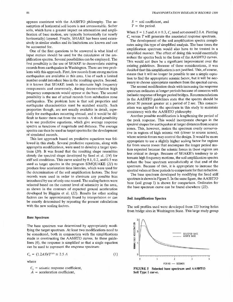
The base spectrum developed by modifying the Seed stiff spectrum is shown in Figure 5. In the same figure, the AASHTO base (soil group I) is shown for comparison. Ordinates for the base spectrum curve can be found elsewhere (22).

Soil Amplification Spectra

The soil profiles used were developed from 123 boring holes from bridge sites in Washington State. This large study group

SELECTED BASE AASHTD BAS[

PER I 00 --- SECONDS

FIGURE 5 Selected base spectrum and AASHTO Soil Type I curve.

Tsiatas et al.

was used in an attempt to include the range of soil types and variations encountered in this area. The properties of all these profiles can be found elsewhere (22).

Input requirements for SHAKE include strain versus shear modulus and strain versus damping curves. For cohesionless soils, curves developed by Seed and Idriss (23) were used (Figure 6). The shear modulus relates to the K2 parameter given in Figure 6 according to the following:

(2)

where K 2 is a function of the void ratio and strain amplitude , and rJ"'" is the effective mean principal stress. For the case of clays, shear modulus and damping curves developed by Seed and Idriss (23) were also used (Figure 7) . This figure indicates that the shear modulus is normalized with respect to un­drained shear strength.

The soils were categorized as clays or sand depending on their predominant behavior , as required for the input to SHAKE. Because the type of information available on the logs is limited, it was necessary to use empirical relations between the available data [usually Standard Penetration Tests (SPT) and undrained shear strength] and dynamic properties of the soil. The following relationship for uncorrected blow counts from work by Ohsaki and Iwasaki (24) , was chosen because it is correlated to down-hole velocity studies , the correlation coefficient is high, and the results are intermediate when compared with the results of other researchers.

Gmax = 1.47N·68 (tsf)

K,

o ~~~-'-~~---''"-~~~~~-'

28

I-~ 24 u

"' UJ 20 0..

0 16

~ "' 12 \.!> z Ci: ::;; ;:§ 4

lo-•

-0 io-•

io-' io-2

SHEAR STRAIN • PERC ENT

/ /

/ /

,/ v

----io -' io- 2

SHEAR STRAIN · PERCENT

FIGURE 6 Shear modulus for sands (top); damping ratio for sands (bottom).

(3)

L

10'"-~~~~~-'-~~~~~---''--~--'

io-•

1-ffi 30 u

"' UJ 0..

0 20

~ "' \.!> z Ci: 10 ::;; <C 0

o io-•

io-' 10

SH EAR STRAIN - PERCENT

/ v

/ /

/

---- io-• io- 1 10

SHEAR STRAIN · PERCENT

FIGURE 7 Shear modulus for saturated clays (top); damping ratio for saturated clays (bottom).

87

It should be noted that using such empirical correlations re­quires caution. Many factors can affect the blow counts re­corded and undrained shear strength test results . The values seen in the boring logs exhibited significant variability, even in apparently homogeneous deposits. Sensitivity studies were performed in an attempt to bracket the possible response, and it appears that the profile responses are not sensitive to minor variations in calculated shear modulus values except at soft sites . These soft sites fall into groups that incorporate a wide range of frequency amplification , accounting for this greater variation .

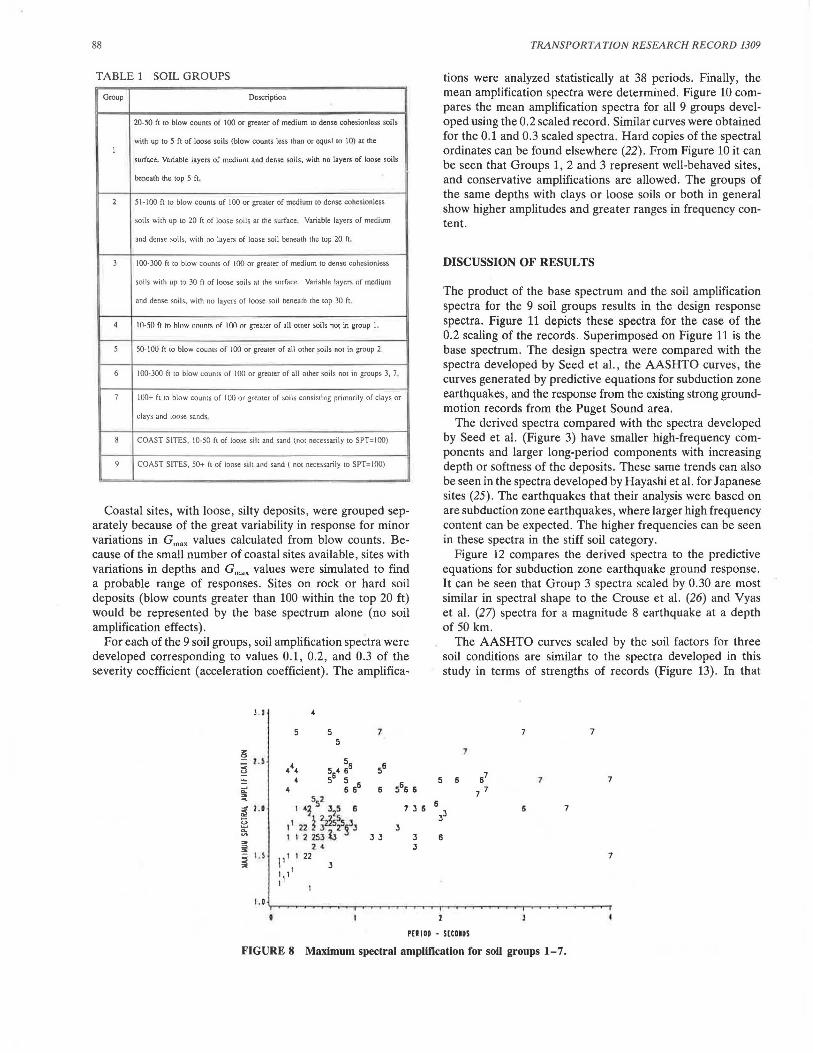
The four simulated records scaled by 0.1 , 0.2, and 0.3 were used with SHAKE to determine the 5 percent damped ac­celeration response of the soil profiles . This response was divided by the response of the time history at a rock out­cropping. The result is a soil amplification spectrum that shows the amplification (or attenuation) effects of the profile on the underlying base motion. The spectra developed with the 0.2 scaled simulation were used to determine groupings . The as­sumption made was that groupings obtained using the 0.1 and 0.3 scaled records would be the same as those developed using the 0.2 records. Peak spectral amplification for each site was plotted as a function of period , and preliminary groupings were made. Sites within each group were analyzed for simi­larities. The results appeared to be primarily functions of depth and types of soils in the profiles. Some slight shifting between the preliminary groups allowed categorization by easily identifiable traits. The final groups are presented in Table 1. Figures 8 and 9 show peak amplification versus period for sites in each group.

88

TABLE 1 SOIL GROUPS

Group Description

20-50 ft m blow counts of 100 or greater of medium to dense cohcsionless soils

with up to 5 ft of loose so ils (blow counts less than or equal to 10) at the 1

surlace_ Variable layers of medium and dense soils, with no layers of loose soils

beneath the top 5 ft.

2 51-100 ft 10 blow counts of 100 or greater of medium'° dense cohesionless

soils with up to 20 ft of loose soils at the surface. Variable layers of medium

and dense soils, with no layers of loose soil beneath the top 20 ft.

3 100-300 ft to blow counts of 100 or greater of medium to dense cohcsionless

soi ls with up 10 30 ft of loose soils al th~. ~urfac.r. Variahle layr:rs of medium

and dense soils, with no layers of loose soil bcne\lth the top 30 ft ,

4 10->0 fr ro hlnw r.m inr.< nr 100 nr grearer or all other soils not in &roup 1.

5 50-100 ft to blow counts of 100 or gr~ater of all other ~oils not in group 2.

6 JOO.JOO ft to blow t.:ounts of 100 or greater of all mher soils not in groups 3, 7 .

7 100+ ft lo blow counts of 100 or greater of soi ls consisting primarily of clays or

clays and loose sands.

8 COAST SITES, 10-50 rt of loose sill and sand (nor necessarily 10 SPT=IOO)

9 COAST SITES, 50+ fl of loose silt and sand (not necessarily co SPT=IOU)

Coastal sites, with loose, silty deposits, were grouped sep­arately because of the great variability in response for minor variations in Gmax values calculated from blow counts. Be­cause of the small number of coastal sites available, sites with variations in depths and Gmax values were simulated to find a probable range of responses. Sites on rock or hard soil deposits (blow counts greater than 100 within the top 20 ft) would be represented by the base spectrum alone (no soil amplification effects).

For each of the 9 soil groups, soil amplification spectra were developed corresponding to values 0.1, 0.2, and 0.3 of the severity coefficient (acceleration coefficient). The amplifica-

l . O 4

5 7 5

z: ~ u s - 4

44 56 ~ 5 4 66

~ • 56 s

s66 6 ~ 4 6 6

6 6 a..

~ 5 2

~ l . O I 4~ 5 J2S B 7 J 6

11 22 3 ~i3s~sf J J e; l\22SJiJ J J J

"' "' 2 • J :!! L$ I'' 1 22 ~

1 11 J

,1

s

6

TRA NSPORTATION RESEA RCH R ECORD 1309

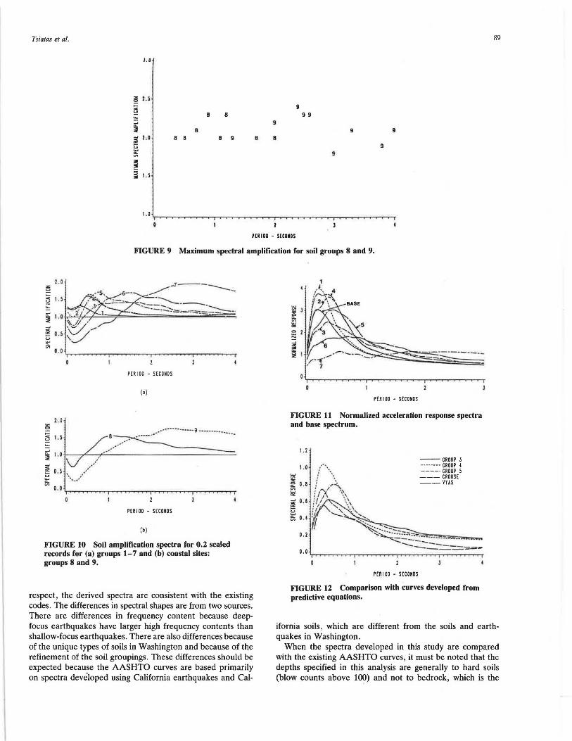
tions were analyzed statistically at 38 periods. Finally, the mean amplification spectra were determined. Figure 10 com­pares the mean amplification spectra for all 9 groups devel­oped using the 0.2 scaled record . Similar curves were obtained for the 0.1 and 0.3 scaled spectra. Hard copies of the spectral ordinates can be found elsewhere (22). From Figure 10 it can be seen that Groups 1, 2 and 3 represent well-behaved sites, and conservative amplifications are allowed. The groups of the same depths with clays or loose soils or both in general show higher amplitudes and greater ranges in frequency con­tent.

DISCUSSION OF RESULTS

The product of the base spectrum and the soil amplification spectra for the 9 soil groups results in the design response spectra. Figure 11 depicts these spectra for the case of the 0.2 scaling of the records. Superimposed on Figure 11 is the base spectrum. The design spectra were compared with the spectra developed by Seed et al., the AASHTO curves, the curves generated by predictive equations for subduction zone earthquakes, and the response from the existing strong ground­motion records from the Puget Sound area.

The derived spectra compared with the spectra developed by Seed et al. (Figure 3) have smaller high-frequency com­ponents and larger long-period components with increasing depth or softness of the deposits. These same trends can also be seen in the spectra developed by Hayashi et al. for Japanese sites (25). The earthquakes that their analysis were based on are subduction zone earthquakes , where larger high frequency content can be expected. The higher frequencies can be seen in these spectra in the stiff soil category.

Figure 12 compares the derived spectra to the predictive equations for subduction zone earthquake ground response. It can be seen that Group 3 spectra scaled by 0.30 are most similar in spectral shape to the Crouse et al. (26) and Vyas et al. (27) spectra for a magnitude 8 earthquake at a depth of 50 km.

The AASHTO curves scaled by the soil factors for three soil conditions are similar to the spectra developed in this study in terms of strengths of records (Figure 13). In that

7

7

6 67 7 7

7 7

JJ 6 7

6

7

m100 - mom

FIGURE 8 Maximum spectral amplification for soil groups 1-7.

Tsiatas et al. 89

J. D

9 8 B 9 9

9 8 9 9

~ 1. 0 8 8 8 g 8 8 9

~ 9

PUIOO - SICGIDS

FIGURE 9 Maximum spectral amplification for soil groups 8 and 9.

~ 1.0.J,::...£/.,,,L.,C=.~~~.;::====;=:=-..;.;;;;;.;.;;;;;.;.;;;_..,=::===. < ~ II •

l u~/ "' o .o.....,_~~~~~~~~~~~~~~~...-.-~

PER I OD - SECONDS

(•)

2. 0 :z !:::! ,_

8 < 1. S ~ !::: ~ c.. l.O ~ ~ < ~ o.s ~ c..

"' 0.0

PERIOD - SECONDS

(b)

FIGURE 10 Soil amplification spectra for 0.2 scaled records for (a) groups 1-7 and (b) coastal sites: groups 8 and 9.

respect, the derived spectra are consistent with the existing codes. The differences in spectral shapes are from two sources. There are differences in frequency content because deep­focus earthquakes have larger high frequency contents than shallow-focus earthquakes. There are also differences because of the unique types of soils in Washington and because of the refinement of the soil groupings. These differences should be expected because the AASHTO curves are based primarily on spectra developed using California earthquakes and Cal-

PER I OD - SECONDS

FIGURE 11 Normalized acceleration response spectra and base spectrum.

l.l --GROUP J --------GROUP I ----· GROUP l --- CROUSE --VYAS

PER I OD - SECONDS

FIGURE 12 Comparison with curves developed from predictive equations.

ifornia soils , which are different from the soils and earth­quakes in Washington.

When the spectra developed in this study are compared with the existing AASHTO curves, it must be noted that the depths specified in this analysis are generally to hard soils (blow counts above 100) and not to bedrock, which is the

90

'1 (\ I \ l· ,,... ... \

. \\ l fi '.;'\

f - ~

-- A!SHTO !YP[ I --------am ALON[ --- CROUP I • BAS[

-- AASHTO TYP[ 11 ----·· CROU P 2 • BIS[ --- CROUP 3 • BAS[

-···· -·~··-·-··-- ·-qm™™=

-- AASHIO TYPE 111 -·---·- CROUP I • am --GROUPl •BAS[ --GROUP7 •BAS£

, ... --··~ . .. .. \ l / ---....,

I v~·_.:.:·· ~~-~---::'..::.~:::.§:-~-7""~-7""~-=-~-::-~_-;-~.-=====-=~

P[R I OD - S[CONOS

FIGURE 13 Comparison of AASHTO curves to spectra developed in this study.

depth prescribed by the AASHTO guidelines. The depth from hard soils to bedrock soils varies from zero to around 900 ft in Washington. The AASHTO spectrum for stiff soil sites (Group 1) generally corresponds to the base spectrum and Group 1 of this study. Larger high-frequency components exist in the spectra from this study. This is consistent with studies showing subduction zone ground motions having larger high frequency content. The spectra are similar above a period of about 1 sec. The AASHTO spectrum for stiff clays and deep cohesionless soils (Group II) corresponds to the groups 2 and 3 spectra in this study. These groups do not include clays, which would generally reduce the higher frequency re­sponse. The AASHTO spectrum for soft to medium-stiff clays and sands would include groups 5, 6 an<l 7 of lhis slu<ly. The average of these spectra would be close to the AASHTO guideline curves . These comparisons show that the results of this analysis are generally consistent with existing spectra in terms of strengths. They also address the soil and earthquake factors in Washington more realistically.

The spectra can also be compared with the responses of the 1949 and 1965 Puget Sound earthquakes. The recording site in Olympia for the 1949 and 1965 events can be classified as a Group 3 site (28). Scaled Group 3 spectra are compared with the responses from these two events in Figure 14. This actual response is enveloped fairly well by the Group 3 spectra except for the high frequency response of the 1965 record. This event was almost directly under the recording station. Because of this , the time history may be rich in high frequency components that would not be seen elsewhere. The recording site in Seattle for the 1965 event would be classified as a Group

0. 7

0. 7

~ 0.6 z ~ 0.5

~a . • ~

< g a.1. e:; 0. 2 '

0 . 1

TRANSPORTATION RESEARCH RECORD 1309

P£R I DD - S£CD NDS

(•)

0 . 0.,..,..,...,...,......,...,.....,....,...__,,..,.......,..,...,...,...,............,,....,,..,.....,...,...~~ ....... -r-T'T

P[R I 00 - S£CONOS

(b)

FIGURE 14 Comparison with Puget Sound earthquakes recorded in Olympia: (a) Group 3 soils scaled by 0.3 and 0.2 and the 1949 event; (b) Group 3 soils scaled by 0.1 and 0.15 and the 1965 event.

1 site. The response at this site is enveloped fairly well by the predicted spectra scaled by 0.10 as shown in Figure 15.

CONCLUSIONS

A base spectrum and soil amplification spectra are developed to be used in seismic design considerations of highway bridges in Washington State. In summary, the following steps are required to use the present results: (a) determine the soil profile and the acceleration coefficient for the site, (b) find base spectrum ordinate for period of interest, (c) find the soil amplification ordinate for period of interest from the spectrum corresponding to the selected soil profile and acceleration coefficient, and (d) the seismic coefficient used in the cal­rnlalions (AASHTO) is then given by: C, = acceleration coefficient x base spectrum ordinate x soil amplification ordinate. The appropriate severity coefficient can be taken

..... "' z

0. 4

~ O.J

~ 0.2

'-' ~ 0. 1

P[R I 00 - S[CONDS

FIGURE 15 Comparison of spectra for Group 1 soils scaled by 0.10 and 0.05 to 1965 earthquake recorded in Seattle.

Tsiatas et al.

from the map of velocity-related accelerations developed by Higgins et al. (12) until the remapping is accomplished. When the results of the present study are used in conjunction with a computer program, such as SEISAB, for earthquake anal­ysis of bridges, a library design response spectra must be introduced into the program. The base spectrum ordinates should be multiplied by all derived spectra. Twenty-seven design response spectra will result, which correspond to the nine soil profiles and the three severity coefficients for each soil profile. The digitized data included elsewhere in work by Tsiatas et al. (22) can be easily used for this purpose.

Although the base spectrum and soil amplification spectra developed in this study are in general agreement with the existing codes in terms of strengths of ground shaking, dif­ferences in spectral shapes are seen. These differences are consistent with expected differences in frequency content be­tween shallow- and deep-focus earthquakes. The soils in Washington are diverse, making it logical to divide the types into more groups than those identified by the existing codes. The spectral amplification and attenuation characteristics of these soil groups, however, correspond fairly well with the site-response characteristics of less refined groupings. The most substantial differences between the existing codes and results of this study are at the higher frequencies (periods less than 0.4 sec). This means the greatest changes in design forces calculated will be to stiff structures or in the trans­verse direction in long-span bridges. For other periods of interest, the spectra developed here may provide a slightly higher or lower (but hopefully more reasonable) value of relative ground-shaking.

ACKNOWLEDGMENT

The work on which this report is based was supported by WSDOT and FHWA, U.S. Department of Transportation. Grateful acknowledgment is made to representatives of var­ious departments of WSDOT, in particular to Bill Carr, plan­ning, research, and public transportation; Dick Stoddard, bridges and structures; and Todd Harrison, geotechnical.

REFERENCES

1. R. S. Crossen. Review of Seismicity in the Puget Sound Region from 1970 through 1978. U.S. Geological Survey Open-File Re­port 83-19, 1983.

2. N. H. Rasmussen, R. C. Millard, and S. W. Smith. Earthquake Hazard Evaluation of the Puget Sound Region, Washington State. Geophysics Program, University of Washington, Seattle, 1975.

3. T. H. Heaton and S. H. Hartzell. Source Characteristics of Hy­pothetical Subduction Earthquakes in the Northwestern United States. Bulletin of the Seismological Society of America, Vol. 71, No. 3, June 1986, pp. 675-708.

4. Guide Specifications for Seismic Design of Highway Bridges. AASHTO, Washington, D.C., 1983.

5. Tentative Provisions for the Development of Seismic Regulations for Buildings. Publication ATC 3-06. Applied Technology Coun­cil, 1978.

6. Seismic Guidelines for Highway Bridges. Publication ATC-6. Ap­plied Technology Council, Redwood City, Calif., Oct. 1981.

7. J. J. Taber and S. W. Smith. Seismicity and Focal Mechanisms Associated with the Subduction of the Juan de Fuca Plate Be­neath the Olympic Peninsula, Washington. Bulletin of the Seis­mologic Society of America, Vol. 75, No. 1, Feb. 1985, pp. 237-249.

91

8. M. G. Hopper et al. A Study of Earthquake Losses in the Puget Sound, Washington Area. U.S. Geological Survey Open-File Re­port 75-375, 1975.

9. S. T. Algermissen and D. M. Perkins. A Probabilistic Estimate of Accelerations in Rock in the Contiguous United States. U.S. Geological Survey Open-File Report 76-416, 1976.

10. D. M. Perkins et al. Probabilistic Estimates of Maximum Seismic Horizontal Ground Motion on Rock in the Pacific Northwest and the Adjacent Outer Continental Shelf. U.S. Geologic Survey Open­File Report 80-471, 1980.

11. P. B. Schnabel and H. B. Seed. Accelerations in Rock for Earth­quakes in the Western United States. Bulletin of the Seismologic Sociely of America, Vol. 63, No. 2, April 1973, pp. 501-516.

12. J. D. Higgins, R. J. Fragaszy, and L. D. Beard. Seismic Zona/ion for Highway Bridge Design in Washington. Washington State Department of Transportation, 1988.

13. T. H. Heaton and S. H. Hartzell. Earthquake Hazards on the Cascadia Subduction Zone. Science, Vol 236, April 1987, pp. 162-168.

14. H. B. Seed, C. Ugas, and J. Lysmer. Site-Dependent Spectra for Earthquake Resistant Design. Bulletin of the Seismological Society of America, Vol. 66, No. 1, Feb. 1976, pp. 221-234.

15. P. B. Schnabel, J. Lysmer, and H. B. Seed. SHAKE, A Com­puter Program for Earthquake Response Analysis of Horizontally Layered Sites. EERC 72-12. Earthquake Engineering Research Center, University of California, Berkeley, Dec. 1972.

16. C. Y. Chang and M. S. Powers. Empirical Data on Spatial Var­iation of Earthquake Ground Motion. Second International Con­ference on Soil Dynamics and Earthquake Engineering, The Queen Elizabeth II, New York to Southampton, Vol. 1, June/July 1985, pp. 3-17.

17. K. Kanai. Engineering Seismology, University of Tokyo Press, 1983.

18. W. B. Joyner and D. M. Boore. Measurement, Characterization and Prediction of Strong Ground Motion. Earlhquake Engineer­ing and Soil Dynamics II-Recent Advances in Ground Motion Evalualion. Geotechnical Special Publication No. 20, ASCE, New York, N.Y., June 1988, pp. 43-102.

19. T. C. Hanks and D. A. Johnson. Geophysical Assessment of Peak Accelerations. Bulletin of the Seismological Sociely of Amer­ica, Vol. 66, No. 3, June 1976, pp. 959-968.

20. C. Ho, K. Kornher, and G. Tsiatas. Ground Motion Model for Puget Sound Cohesionless Soil Sites. Earthquake Spectra, May 1991.

21. D. A. Gasparini and E. H. Vanmarcke. Simulaled Earthquake Molions Compatible with Prescribed Response Spectra. Report R76-4. Massachusetts Institute of Technology, Jan. 1976.

22. G. Tsiatas, R. Fragaszy, C. Ho, and K. Kornher. Design Re­sponse Spectra for Washington State Bridges. Final Technical Re­port. Washington State Department of Transportation, May 1989.

23. H. B. Seed and I. M. Idriss. Soil Moduli and Damping Factors for Dynamic Response Analysis. Report No. EERC 70-10. Earth­quake Engineering Research Center, University of California, Berkeley, 1970.

24. Y. Ohsaki and R. Iwasaki. On Dynamic Shear Moduli and Pois­son's Ratio of Soil Deposits. Soils and Foundations, Japanese Society of Soil Mechanics and Foundation Engineering, Vol. 13, No. 4, Dec. 1973, pp. 61-71.

25. S. Hayashi, H. Tsuchida, and E. Kurata. Average Response Spec­Ira for Various Subsoil Conditions. Third Joint Meeting, U.S.­Japan Panel on Wind and Seismic Effects, UJNR, Tokyo, Japan, May 10-12, 1971.

26. C. B. Crouse, Y. K. Vyas, and B. A. Schell. Ground Motions from Subduction Zone Earthquakes. Bulletin of the Seismologic Society of America, Vol. 78, No. 1, Feb. 1988, pp. 1-25.

27. Y. K. Vyas, C. B. Crouse, and B. A. Schell. Regional Desig11 Ground Motion Criteria for the Southern Bearing Sea . Seventh lnlernational Conferences on Offshore Mechanics and Arclic En­gineering, Houston, Tex., Feb. 7-12, Vol. I, 1988, pp. 187-193.

28. Geotechnical and Strong Motion Earthquake Data from U.S. Ac­celerograph Stations. NUREG/CR-0985. Shannon and Wilson, Inc., and Agbabian Associates, Vol. 4.

Publication of this paper sponsored by Committee on Soil and Rock Properties.