a N

MISCELLANEOUS PAPER GL-85-1

SEISMIC DESIGN OF GRAVITYof EngineerRETAINING WALLS

by

Robert V. Whitman, Samson Liao

Department of Civil Engineering F 0

Massachusetts Institute of Technology

Lf 77 Massachusetts Avenue(%J Cambridge, Massachusetts 02139

.2g 5g- .5g

DTIGN ELECTE

0.5 Al3 DE

.. ~O 2 gAPR 12 985

15q Approved for Public Release. Distribution Unlimited

US g Anuay 1985s AfEgnes.--- •

0.259

~2gXO.39 Em.

LLS

Prepared for DEPARTMENT OF THE ARMYUS Army Corps of EngineersWashington, DC 20314-1000

Under CWIS Work Units 31173 and 31589 _Monitored by Geotechnical Laboratory

US Army Engineer Waterways Experiment StationP0 Box 631, Vicksburg, Mississippi 39180-0631

....2 ;- .

. ... . . ._. _., _'• •. ,•. _._• ,_,- , . _._..:. _-, - : • , . ,, -, , . .. . -, . .. _ ,, . -,_', -• -.._',.-,.,,,., ,_,._,._.,. '_,l: -..

Destroy this report when no longer needed. Do not returnit to the originator.

o .

The findings in this report are not to be construed as an officialDepartment of the Army position unless so designated

by other authorized documents.

The contents of this report are not to be used foradvertising, publication, or promotional purposes.Citation of trade names does not constitute anofficial endorsement or approval of the use of

such commercial products.

... . .......... . . . . . . . . .. .

• . . ., f

UnclassifiedSECURITY CLASSIFICATION OF THIS PAGE (*%hen Data Entered) .__ _

REPO•RT DOCUMENTATION PAGE READ INSTRUCTIONSBEFORE COMPLETING FORM1.REPORT NUMBER 2. GOYJ ACCESSION No.3. RE c IP IEN AALOG NUMBER - -

Miscellaneous Paper GL-85-1 /lZ/4. TITLE (and Sublitt) 5. TYPE OF REPORT & PERIOD COVERED

SEISMIC DESIGN OF GRAVITY Final reportRETAINING WALLS

6. PERFORMING ORG REPORT NUMBER

7. AUTHOR(e) 8. CONTRACT OR GRANT NUMBER(.)

Robert V. Whitman, Samson Liao

9. PERFORMING ORGANIZATION NAME AND ADDRESS 10. PROGRAM ELEMENT. PROJECT, TASKAREA & WORK UNIT NUMBERS

Department of Civil Engineering CWIS Work Units 31173Massachusetts Institute of Technology and 31589Cambridge, Massachusetts 02139

11. CONTROLLING OFFICE NAME AND ADDRESS 12. REPORT DATE

DEPARTMENT OF THE ARMY January 1985US Army Corps of Engineers 13. NUMBER OF PAGES

Washington, DC 20314-1000 15614. MONITORING AGENCY NAME & ADORESS(II different from Controlling Office) 15. SECURITY CLASS. (of this report)

US Army Engineer Waterways Experiment Station

Geotechnical Laboratory UnclassifiedPO Box 631, Vicksburg, Mississippi 39180-0631 aIS. DECLASSIFICATION/DOWNGRADING . -

SCHEDULE

16. DISTRIBUTION STATEMENT (of this Report)

Approved for public release; distribution unlimited.

. .1

1. DISTRIBUTION STATEMENT (of the abstract entered InBlock 20, It different from Report) "'{ •

IS. SUPPLEMENTARY NOTES

Available from National Technical Information Service, 5285 Port Royal Road,Springfield, Virginia 22161.

19. KEY WORDS (Conlinue on reverse side if necesary tnd Identify by block number)

Retaining walls--design and construction (LC)'

Richards-Elms retaining wall design method (WES).

20. ADSTIR ACT ( s ss reverse as If necessary and fdeitfy by bl ock . .bor

--- - The report discusses the seismic design of gravity walls retaining granularbackfill without pore water. The general features of behavior are illustrated

by field experiences, results from laboratory model tests and from theoreticalanalyses. Both the conventional method of design and the Richards-Elms method,based upon n1c analogy to a sliding block, are reviewed. A shortcoming of thesliding block analogy is discussed, and corrections obtained using a two-blockmodel are presented. Several sources of uncertainty are examined in detail: -

(continued)

DD IjR fM 1473 EDITION OF I OV 6SIS OSSOLEE Tnlii EeiX AtN 74T Umoo .vsSmorztnclojsified

SECURITY CLASSIFICATION OF THIS PA ,F INWen Vats Fterrd)

. --. . ... " i - . i ' - . . . . . . l 2 . ....

7..

UnclassifiedSECURITY CLASSIFICATION OF TNIS PAGE(fWan Data Enterd) I- "

20. ABSTRACT (Continued)

"he random nature of ground motions, uncertainty in resistance parameters, and

model errors, including the important influence of deformability in the back-

fill. All of these results are then combined to develop a probabilistic method

for predicting seismically induced displacements of walls and an improvedversion of the Richards-Elms method of design. The risk that walls designedby the conventional method might experience excessive displacements is _

analyzed. .' ,,, -"" .-.

Unlssf-

S

• -0 L'

- .-

~.0 .

Unclassified"]- ]"I

SECURtITY CLASSIFICATION OF THIS PAGE(WI,.n 0.,. Elt.,.d) ""'

.'..- . •• -.-. --- -- ,.-. : •'.-. .. .'.-.". ."...... " .. ..-- .- .- .".-..";i'-',----"

, * - .. ,

PREFACE

This report was prepared by Professor Robert V. Whitman and

Mr. Samson Liao of the Department of Civil Engineering, Massachu-

setts Institute of Technology, Cambridge, Massachusetts, under

Purchase Order No. DACW39-83-M-2088 with the US Army Engineer

Waterways Experiment Station (WES). The work was conducted during

the period April-December 1983 and was jointly sponsored by the . -

Office, Chief of Engineers (OCE), US Army Civil Works Investiga- -

tion Studies, "Computer-Aided Engineering Software," CWIS Work

Unit 31589, and "Special Studies for Civil Work Soils Problems,

CWIS Work Unit 31173. The respective OCE Technical Monitors

were Messrs. Lucian G. Guthrie and Richard F. Davidson, respec-

tively. Dr. P. F. Hadala, Assistant Chief, Geotechnical

Laboratory (GL) was the WES Technical Monitor. The work was

under the general direction of Dr. W. F. Marcuson III, Chief, GL.

COL Tilford C. Creel, CE, and COL Robert C. Lee, CE, were

the Commanders and Directors of WES during the period of this

study. Mr. F. R. Brown was Technical Director.

\AurcCZiofl ForUTIS GFA&T

""i Tn--'•in iorn "

.Vv .,- . -. .

' ,: ,;t ', " Codes --

o.r -. -

, .10

................................................. "..... -......... •..

0

ii

TABLE OF CONTENTS .

Page

1. INTRODUCTION 1

2. GENERAL FEATURES OF DYNAMIC BEHAVIOR 4

2.1 Complex Behavior and Simplified Models 40

2.2 Field Observations 5

2.3 Model Experiments 7

2.4 Finite Element Results 14

3. CONVENTIONAL DESIGN 20

3.1 General Concepts 20

3.2 Evaluating Dynamic Earth Pressure 23

3.2.1 Mononobe-Okabe Equation 23 "°-

3.2.2 Validity of the Mononobe-Okabe 27Equation

3.3 Discussion of the Seismic Coefficient Method 29

3.3.1 Format of Typical Seismic Coefficients 29

3.3.2 Comparison of Two Seismic Coefficient Maps 30

3.3.3 Judgement in Formulation and Use 33 -

3.3.4 Seismic Coefficients and Safety Factors 33

3.3.5 Conclusion on Seismic Coefficients 35

4. RICHARDS-ELMS METHOD 36

4.1 General 36 .

4.2 Newmark's sliding Block Model 36

4.3 Evaluating Retaining Wall Displacements 43

4.4 Richards-Elms Design Procedure 46

4.5 Comments on the Richards-Elms Method 47

i l' --i '. 2-'l~ .. ii i ' i . ...- .- :? l- i -: . . .. .' --. - .. . - -. . ."ii .i -.. "- '. ... " i. . '. - i ,i. ":- -

5. KINEMATIC CONSTRAINTS UPON MOTION OF BACKFILL 52

5.1 The Two-Block Model 52

5.2 Comparison with Single-Block Model 54

5.3 Numerical Results 58

5.4 Comparison with Experimental Results 61

5.5 Summary 65

6. RANDOM NATURE OF GROUND MOTIONS 66

6.1 Introduction 66

6.2 Scaling of Records 67 .

6.3 Orientation Effects 70 -

6.4 Scatter Among Different Sites and Events 72

6.5 Effect of Vertical Accelerations 74 S

6.6 Combined Uncertainty 78

6.7 Predicting Residual Displacements 82

6.8 Application to Retaining Walls 85 e

6.9 Improvements to Predictions 86

7. UNCERTAINTY IN RESISTANCE PARAMETERS 87

7.1 Introduction 87

7.2 Uncertainty in Friction Angle 88

7.3 Block on Horizontal Plane 89

7.4 Retaining Walls 94

8. MODEL ERRORS AND UNCERTAINTIES 100

8.1 Failure Plane Inclination 100 -

8.2 Elastic Backfill Effects 105

8.3 Tilting i11

. . -. .

iv

Page

8.4 Approximations to 2-Block Analysis 115

9. IMPROVED APPROACH TO DESIGN 118

9.1 Review of Objectives 118

9.2 Equation for Predicting Motions 118

9.3 Approach to Design Using Safety Factor 125Against Displacement

9.3.1 Choice of safety factor 130

9.3.2 Examples 131

9.4 Reliability Implicit in Other Design 131 SApproaches

9.4.1 Conventional design 132

9.4.2 Design following Richards-Elms 133

9.5 General Discussion 135

10. CONCLUSIONS AND OPPORTUNITIES 141

10.1 Conclusions 141 .

10.2 Opportunities 142

REFERENCES 144

LIST OF SYMBOLS 147

APPENDIX A 151

0-;<.

_S

'9:

• -": . i . .- .:- i 2 - 2 " -•2 • i- 2 2 2- . ' - .- .-. .. . ..- i - . - ' - - . . ... ° .- - . .- .- , - " .i " - .. . ' i

1 INTRODUCTION 0

The design of gravity retaining walls in an earthquake-prone

environment is usually based upon static analysis using an

equivalent seismic coefficient. This can be a suitable approach,

provided that the seismic coefficient is determined from a

rational analysis of actual dynamic behavior.,However, the use of

seismic coefficients in current practice is largely empirical and

sometimes inconsistent, leading to designs that may be either

excessively conservative or unsafe.

In 1969, Richards and Elms presented a rational method for

the selection of a suitable seismic coefficient, based upon the

concept of an allowable permanent displacement. This approach is

generally compatible both with the design philosophy used to

design gravity retaining walls against static loads and with that

used to design many other structures against earthquake loads.

Richards and Elms utilized an analogy between the behavior of a

gravity retaining wall and that of a block sliding on a plane,

which is an oversimplification of the actual behavior of a wall-

backfill system. Consequently, they suggested the use of a

liberal safety factor, which to some extent takes into account the

effects of these oversimplifications and other uncertainties in

the analysis.

The work described in this report improves upon and extends

the Richards-Elms approach to design by considering corrections to

the simple sliding block analogy, and by introducing a rational

basis for the selection of a suitable safety factor for use in the

• . • . • . . ... . . • . - .- . . , .

2

approach. The essence of the proposed method is the following

expression for prediction of the residual displacement experienced

by a gravity retaining wall during an earthquake:

d Rw Rv R2/1 Q * R (1.)

where d Rw is the predicted residual displacement 0

is the mean (expected) residual displacement for aRv

sliding block exposed to ground motion characterized by

a small number of parameters (such as peak acceleration

A and peak velocity V).

R2/1 is a deterministic term accounting for a specific

kinematic deficiency in the single sliding block model.

Q is a term accounting for the unpredictable details in

the random nature of future earthquake shaking.

R is a term accounting for the uncertainty in the

parameters characterizing the backfill, wall and

foundation soil.

M is a term accounting for other, and as yet, poorly

understood deficiencies of the simple sliding block 0

model.

-•ot-9

3

The scope of this report is restricted to gravity retaining

walls with granular backfills subjected to earthquakes, where soil

liquefaction is not of importance. It also primarily deals with

the translational mode of retaining wall movements, treating

rotational movements as a secondary concern. Chapter 2 presents

an overview of the complex nature of the dynamic retaining wall

problem, and Chapter 3 discusses the conventional approach to

design. Subsequent chapters treat and discuss each of the

individual terms in Equation 1.1 in detail.

It should be noted that further research and development

remains to be done to render the basic Richards-Elms procedure

completely satisfactory. Nevertheless, based on the present

knowledge summarized in this report, an improved design procedure

is presented in Chapter 9.

S< .i. -

".0 °

4

2- GENERAL FEATURES OF DYNAMIC BEHAVIOR

2.1 COMPLEX BEHAVIOR AND SIMPLIFIED MODELS

Analysis of the behavior of gravity retaining walls during

earthquake loading is a complex soil-structure interaction problem

potentially involving plastic deformations and large strains.

Even with the use of numerical procedures, such as the finite

element method, it is not presently feasible nor possible to

simulate all the phenomenon that would occur. As in all branches

of engineering, simplified models with various approximations and

assumptions are necessary to make complex problems more tractable,

particularly for purposes of design.

Various simplified models, useful for engineering design of

retaining walls, will be presented in subsequent chapters of this

report. In this chapter, the intent is to illustrate and examine

the complexities of retaining wall behavior, and to highlight some

of the major aspects of the problem that have been considered in

the simplified models. However, more importantly, the phenomena

that have not been considered in the simplified models are also

identified, to provide a basis for judging the limitations of the

models.

A general overview of retaining wall behavior is presented

here, based on a review of field observations, laboratory model

experiments, and the results of a relatively sophisticated finite

element model. Further aspects of some particular details of

these observations and data will be discussed, as necessary, in

subsequent chapters.

- •S

18

the earth pressure thrust is the force in the spring (labeled 'A')

connecting the two masses representing the wall and the backfill

wedge.

If the ground is suddenly accelerated to the right and slip

occurs as in Fig. 2.7(c), a force would develop in the spring 'A'

because of differences in the inertia forces between the two

masses and differences in the stiffness of the shear springs.

However, there would be no force in the spring 'B', and so the

force in the spring 'A' would be fairly small, and perhaps even

slightly tensile. On the other hand, when a sudden acceleration

is applied to the left as in Fig. 2.7(d), the force in spring 'B'

is activated to resist the inertia forces of the two masses. As a

result, slip movements do not occur, but a relatively large force

would be present in spring 'A', the analog of the earth pressure.

The above arguments have tried to explain in only a purely

intuitive fashion the complex nature of forces and displacements

in a elastic-plastic retaining wall model. However, the major

point of emphasis as it applies to gravity wall design is that

there is not a clear direct correlation between the maximum earth

pressure force and the amount of relative displacement that

occurs. Focusing too much upon the forces exerted by the backfill

may lead to meaningless results, and it is more essential think in

terms of displacements in design.

The location of the resultant dynamic earth pressure force

was observed to vary with time in a complex manner in the finite

element model. Parametric studies using a finer mesh model (than

that shown in Fig. 2.5), indicated that the time variation of the

S i

17

M-S

(a) Elastic-Plastic Retaining Wall

BS

Shear Springs Axial CompressiveSpring only

71171n711771111ii17-Y , (no tension)

(b) Idealized Lumped Mass System

A BTr

Slip.',__ l . -

-Ground Acceleration

(C) Occurrence of Slip

A B 0

-- Ground Acceleration

(d) No Slip, Elastic Deformations Only

.O

FIG. 2.7 AN INTUITIVE MODEL OF ELASTIC-PLASTIC RETAININGWALL BEHAVIOR.

S. . . . .. .. . . . . . . . .m '.:-' ' ,.; -'. ." m .r,,.l '-'• - " " " " . .".. .".-".. . .".".. . . . .".".. . . .-. ".. ."."".".

16

'i -Slip *Slip -*Slip

~360

'520-

~280 5

240

200 0.5 1.0 1.5 2.0 2.5 3.0i3 2 0** -.-

z280-

~240-

-Sloo ip Slip meSlip -s

0 0.5 1.0 1.5 2.0 2.5 3.0 *-

50 - -Slip.- SlipZ 401-wda 301

-0J

U)

0 0.5 1.0 1.5 2.0 2.5 3.0CYCLE NUMBER

FIG. 2.6 TYPICAL RESULTS FROM FINITE ELEMENT MODEL FORRETAINING WALL SUB3JECTED TO 3 CYCLES OFSINUSOIDAL GROUND MOTION.

15

-• -• .8 m

Backfill properties:.9 /

• , / :30o

H=8m •• o c = 0,otential P 2000 kg/mri 3

S.. " /. -- failure planePc=v . = 0.3

2400 k 0= 54.67" K 0o:: 0.43

(a)

Contact elements with Cn=iE8kN/m/m, Cs=O

Slip elements with Cn=IE~kN/mlm, Cs5 lE5kNImlm

Slip element with Cn =1 E12 kN I/m/m. Rigid boundary 5Cs =IE 5 kNI mlm4my Scale; 4m

Cn= Normal stiffness of slip elements

CS: Shear stiffness of slip elements -0

(b

FIG. 2.5 FINITE ELEMENT MODEL OF A RETAINING WALL(AFTER NADIM, 1982).

..0 .

14

2.4 FINITE ELEMENT RESULTS S

Though even sophisticated finite element analyses are

simplified models of actual behavior, they can nevertheless offer

insight into physical processes that are difficult to observe or

measure experimentally. The finite element idealization of a

retaining wall used in a study by Nadim (1982) is shown in Fig.

2.5. The material properties of this model are linearly elastic,

except for the essentially rigid-plastic elements at the base of

the wall, at the wall-soil interface, and along a preselected

failure plane through the backfill. This model is able to account S

for elastic deformation of the backfill as well as for the

development of a Coulomb-type failure wedge.

A typical set of results, obtzined using 3 cycles of S

sinusoidal motion at the base of the grid, is shown in Fig. 2.6.

There are three intervals (marked "slip" on the figure) during

which the wall slides upon the base. In these intervals, the S

shear force at the base of the wall is constant and the thrust

betwec , backfill and wall is relatively low. On the other hand,

the maximum thrusts from the backfill occur at times when no slip S

is occurring, and when the base shear resistance is fairly low.

An explanation for the lack of direct correlation between the - "

earth pressure force and the amount of wall slippage (at any given

time) is illustrated in Fig. 2.7. Here, the finite element model

is further idealized as a lumped mass system consisting of two

masses and axial and lateral-shear springs. A unique feature

imagined for one of the axial springs (labeled 'B') is its ability

to transmit compressive forces, but not tension. The analog of

-72.. . . . .. ,= .. . . . . . . . . . . . . . .

. . . . . . . . .. . . . . . . . .

13

0.60Slip- -Slipj

CP a4 BaseAcceleration

C

0.2z 0.20 "A Wall"

0 Acceleration 0

's I~ Ad0w0

w0-0.20,

0 0.08 0.16 0.24 0.32 0.40 0.48 0.56 0.64

E TIME in seconds

z46w

w 2p-I , p i..1 I p - ±I '~i 0-

a. 0 0.08 0.16 0.24 0.32 0.40 0.48 0.56 0.64(0TIME in seconds

FIG. 2.4 TYPICAL MEASUREMENTS OF ACCELERATION ANDRELATIVE DISPLACEMENT - IN EXPERIMENT PERFORMEDBY LAI (1979).

(Figure based on reduced data from Jacobsen,1980).

. . . . .-. ..

12

Typical measurements of acceleration and relative displace-

ment of the model wall obtained by Lai (1979) are shown in Fig.

2.4. The first feature to note is that the total slip of the

model retaining wall does not occur in a single movement (i.e.,

catastrophically), but rather occurs in a stepwise fashion as a

series of smaller incremental displacements. During the time

intervals when slip is not occurring, the acceleration of the

model wall follows closely the input base acceleration. The

occurrence of slip is associated with wall accelerations that are

less than the peak base motions, and there appears to be a

critical acceleration at which slip starts to occur. Also, slip

occurs in only the direction away from the backfill, implying that

passive pressures are more than sufficient to resist wall

movements into the backfill.

A problem common to all model tests is the lack of similitude

in stresses and loads from using small scale models. In part, .

this scaling problem can be alleviated by conducting tests in a

centrifuge, as has been reported by Ortiz, et al. (1981) and by

Bolton and Steedman (1982) in their experiments on model retaining

walls. Currently, there is an extensive research program on

retaining walls being carried out at the Cambridge University

Centrifuge facility, but the results of those model tests are not

available to the writers at the time of publication of this

report. It is almost certain that these series of tests will

provide further insight into retaining wall behavior, and may

change some of the conclusions stated here.

" " ' . . . . .. . . . ... . . . .

0

FIG. 2.3 MODEL TEST SHOWING TRANSLATIONAL MODE OFFAILURE (FROM LAI, 1979).

Note: Scale is marked in cm.

10

* The formation of a single predominant failure plane in the

backfill, along which slip occurs.

* A significant amount of backfill settlement.

* The occurrence of distortional shear strains in the

backfill failure wedge.

0 The plastic deformation of the soil in the area near the

toe of the wall as a result of wall rotation.

Lai (1979) performed a series of experiments using L-shaped

model retaining walls approx. 12.6 inches (320 mm) high with a

base width of 8.7 inches (220 mm). The model walls were made of

aluminum, and additional steel plates could be secured to the base

of the wall to vary the total weight of the wall. The dynamic

excitation was provided by a shaking table which could simulate

both periodic and earthquake excitations.

A photograph of one of Lai's model tests after failure is

shown in Fig. 2.3. In contrast to the rotational failures,

translational movements produce very little distortional strain in

the failing backfill soil wedge, and can be approximated as a

rigid body motion. However, plastic deformations of the soil at

the toe of the soil wedge must occur in the process of movement.

Similar to the result shown for rotational failure, Lai noted the

formation of a single predominant failure plane, though other

planes developed in the failing wedge with larger movements.

Also, there is clear evidence that increasing the weight of the

wall leads to flatter inclinations of the failure plane.

• - .••] ,•• [.• .• [• • [[ -[[• •i .ii.. •i .. .. °.. , / • . •.. .• i [ [.-iii.•I i• [ i.i...i•I, .. i " . -. .-.. 0 .

(a) Before startinq test

of gravity wall.

(b) Condition of gravity

wall after l minute

of vibration.

(c) Condition of gravity

wall after 2- minutes2

of vibration.

FIG. 2.2 MODEL TEST SHOWING ROTATIONAL MODE OF FAILURE(FROM MURPHY, 1960).

Note: Scale is marked in inches.

2-

8

"(1970), and more recently by Nadim (1982). Generally, the

experiments that have been performed can be classified into two

groups:

"* Experiments primarily concerned with the measurement of

dynamic earth pressures and/or structural response.

"* Experiments to measure the movements of retaining wall

and observe general failure patterns during shaking.S

The first group, involving experiments to measure dynamic

earth pressure, has had limited success in the comparison of

results with theoretical solutions, in particular the

Mononobe-Okabe equation. Specific details of these comparisons

with theory will be discussed in Chapter 3. It has generally been

observed that the distribution of earth pressure does not increase

linearly with depth as in the case for static pressures. Also,

the location of the resultant of the total force is usually

located above the lower third point along the height of the wall. _

Several of these experiments involved model walls that were fixed

or restrained, and subsequently did not correspond to true field

conditions.

The second group of experiments are generally closer in their

simulation of actual field conditions. Murphy (1960) conducted

tests on a model gravity retaining wall made of solid rubber

shaken with sinusoidal base motion with a period of 1.48 seconds.

Figure 2.2 shows the sequence of failure of the retaining wall.

Although the wall weight is improperly scaled and there are S

undoubtedly frictional effects (i.e. model against glass

container), several significant behavioral features can be noted:

. . .-...--

. ...-. -. .-. .,..-

7

by Nadim (1980), but the results are of a preliminary nature.

Settlements of the backfill behind a wall generally accompany

outward movements of the wall. Evans (1971) reports fill settle-

ments of the order of 10% to 12% of the fill height. Such orders 0

of magnitude of downwards movements of the backfill associated

with outwards movement of the wall are consistent with the concept

of the development of a wedge of soil failing along a plane behind S

the wall.

It has been observed that movements are not always associated

with damage or failure. Evans (1971) noted that of the 39 bridges

examined in the vicinity of the 1968 Inangahua earthquake in New

Zealand, 23 showed measureable movement (without damage), and only

15 were damaged. This is an important concept which is used by S

Richards and Elms (1979) in the proposed design method.

Designing to limit the amount of outward movement is a

rational method to avoid failure not only for the translational

mode, but perhaps also for rotational modes of failure. In the

case of bridge abutments, if the amount of translation is

restricted so that contact and restraint by the bridge S

superstructure is avoided, then the likelihood of rotational

movements about the top of the retaining wall is greatly reduced.

2.3 MODEL EXPERIMENTS

Tests have been performed by a number of investigators using

small scale models of earth retaining structures subjected to

dynamic base motion. Reviews and summaries of the various results

from these experiments have been reported by Seed and Whitman

S.. .... . . .... . ... *- ,. . .. . . . . ..n. . . . .

,-/ i-

.-/I

II ,

/

(a) Outward Translation

;iI•

•(b) Rotation about the Base s-

l• r lIliA\\-

" ~///' I

-/ I

:i:: ~(c) Rotation about the Top .

,'. ' - -

FIG. 2.1 POSSIBLE MOVEMENTS OF GRAVITY RETAINING WALLS.

"j "p

o..i: ... ; i -. iL-. .' •.'-'•.• i.1..-i'.••. ."i'. / '.. .i--, :.ii .i---< -•'-..•.'-' .••.-•• •:•... . .. < .. i- -.

5

2.2 FIELD OBSERVATIONS

Many reports of retaining wall movements during earthquakes

are available in the literature. Useful summaries of these data

have been presented by Seed and Whitman (1970), the Japan Society

of Civil Enginee-s - JSCE (1977), and by Mayes and Sharpe (1981).

Aside from the cases where liquefaction was a cause of

failure, three types of retaining wall movements have been

observed, as schematically illustrated in Fig. 2.1. These are:

* Outward translations of the wall

* Rotations about the base of the wall

* Rotations about the top of the wall

Most cases of movement involve a combination of translation

and rotation. Rotations about the top of the wall appear to be

restricted to retaining walls forming part of bridge abutment

structures. Mayes and Sharpe (1981) suggest that rotation about

the top occurs only after outward motion of the wall brings the

*" top into contact with and restraint by the superstructure.

However, the pattern of overall bridge movement in some cases

indicate that inertia forces from the superstructure may actually

havepushed the top of the wall into the backfill (Evans, 1971).

In the simplified methods presented in subsequent chapters,

only the translational mode of movement is considered in analysis.

This is because translational movements are more analytically

tractable than rotational movements, but it is also an obvious

disadvantage of the methods, since it is rare that purely

. translational movements of walls have been observed. Some

" analytical work on rotational modes of movement has been reported

...........................................

19

location of the earth pressure depended on factors such as the

elastic modulus of the backfill and the frequency and amplitude of

th( input ground motion.

Another feature observed in the finite element model is the

amplification of ground motions due to the elastic properties of

the wall and backfill. Since the system is elastic, a natural

frequency of vibration can be associated with the retaining wall

and the soil. If the input ground motion due to an earthquake has

a central frequency near the natural frequency, effects similar to

resonance will tend to amplify the maximum ground acceleration,

and cause larger displacements of the retaining wall.

- .,

**I -I I I I4U U iIP UL I LIE. *I!* U0 U *-

20

3- CONVENTIONAL DESIGN

3.1 GENERAL CONCEPTS

Gravity retaining walls are typically designed using a static

equivalent earthquake coefficient. This coefficient is used to

evaluate the static plus dynamic force exerted on the wall by the

backfill, and should also be used to calculate the inertia force

due to the wall. A schematic of these forces is shown in Fig.

3.1, along with definitions and notation for the seismic

coefficients. Having found these forces, conventional static

design procedures are followed, which nfeans ensuring that the

weight of the wall, shear resistance on the base of the wall and

passive resistance at the toe are sufficient (with appropriate

safety factors) to resist sliding, overturning and bearing

capacity failure.

In concept, the use of a seismic coefficient (also called the

pseudo-static method of analysis), is equivalent to a static

tilting of the problem at an angle iA computed as:

NS

=tan- NH (3-1)1NV

where N H = the horizontal seismic coefficient

NV = the vertical seismic coefficient

with positive (+) inertia force directions as noted in Fig. 3.1.

* Figure 3.2 illustrates this concept for a simple case where Nv = 0.

•.• -.• ., -;1 .;-i -'i il 'i• . .. .. - "? i. .. [ -• .•. - .• .l-• ..• •. . . • i .; • ii i~ -• • 1" . ..• ?• ~ : -? ; . il . .•~ li • i; < .; .ii • •i .•' . -, i .i .i-Vi

21

Z

iN WT I .il' -Nv ::H " F ailur'e -Plane : NvW

-FW

.W = Weight of Retaining Wall

Ws = Weight of Soil Backfill Wedge .0

NH * Horizontal Seismic Coefficient

Nv = Vertical Seismic Coefficient

FIG. 3.1 SCHEMATIC OF STATIC EQUIVALENT SEISMIC _0COEFFICIENTS AND EARTHQUAKE INERTIA FORCESFOR CONVENTIONAL DESIGN.

...-. ...-. . .-. '.: • --. '. .-. '. -. . .. :.,-,.....' -, ...... - .-.-... '..... -.... .-.. .. . . .....

22

A. "

90

(a) Retaining Wall with Gravitational andHorizontal Seimic Force Vectors

(b) Equivalent Static Problem withGravitational Force Only

FIG. 3.2 INTERPRETATION OF THE IP-ANGLE IN CONVENTIONALSEISMIC COEFFICIENT ANALYSIS (NV 0).

V.

-S

~D

23

As can be readily sec., a logical conclusion from this

interpretation of the angle, T is that T can not exceed the angle

of repose (0) for cohesionless flat backfill (Richard and Elms,

1979). Since the steepest slope that can be formed is at the

angle of repose, T > * would correspond to an impossible non-

equilibrium condition. Similarly, for a backfill inclined at

angle i, T would be restricted to have values less than 4k-i.

Physically, as T increases, the critical angle of the failure

plane becomes flatter, until at T = 0-i, the failure plane becomes

parallel to the backfill slope.S

3.2 EVALUATING DYNAMIC EARTH PRESSURE

3.2.1 Mononobe-Okabe Equation

Although retaining wall seismic stability analyses can be

performed by assuming several trial slip planes of failure in the

backfill (as in slope stability analysis), usually earth pressures.0

are calculated using some version of the Mononobe-Okabe equation

(Mononobe, 1929 and Okabe, 1926). In its complete form, the

equation is written as:

2PAE = 1/2 H (1-Nv) K (3.2.a)

_0

where

cos 2 (-M-8)

COS y [f /sin(•-+6) sin('_Y-i)A COS y cos 2 8 cos('+8+C) 1 + cos(i-8) Cos(•+8+i)

(3.2.b)

.......................................... ... .. ... .. - ....-'

24

BACKFILL PROPERTIES

8 PAE y*Unit Weight

4)uAngle of internalFriction

tail NH

FIG. 3. 3 DEFINITION OF PARAMETERS FOR MONONOBE-OKABEEQUATION.

25

P is the combined active static and dynamic thrust, and theAE

other quantities in the equation are:

y = unit weight of the backfill

H = height of the backfill

S= angle of internal friction of the backfill

6 = angle of friction between the backfill and the wall

= angle of inclination of the back of the wall (with

respect to vertical)

i = angle of inclination of the backfill

The above variables are illustrated in Fig. 3.3. NV and T are as

previously defined (Eqn. 3.1). -

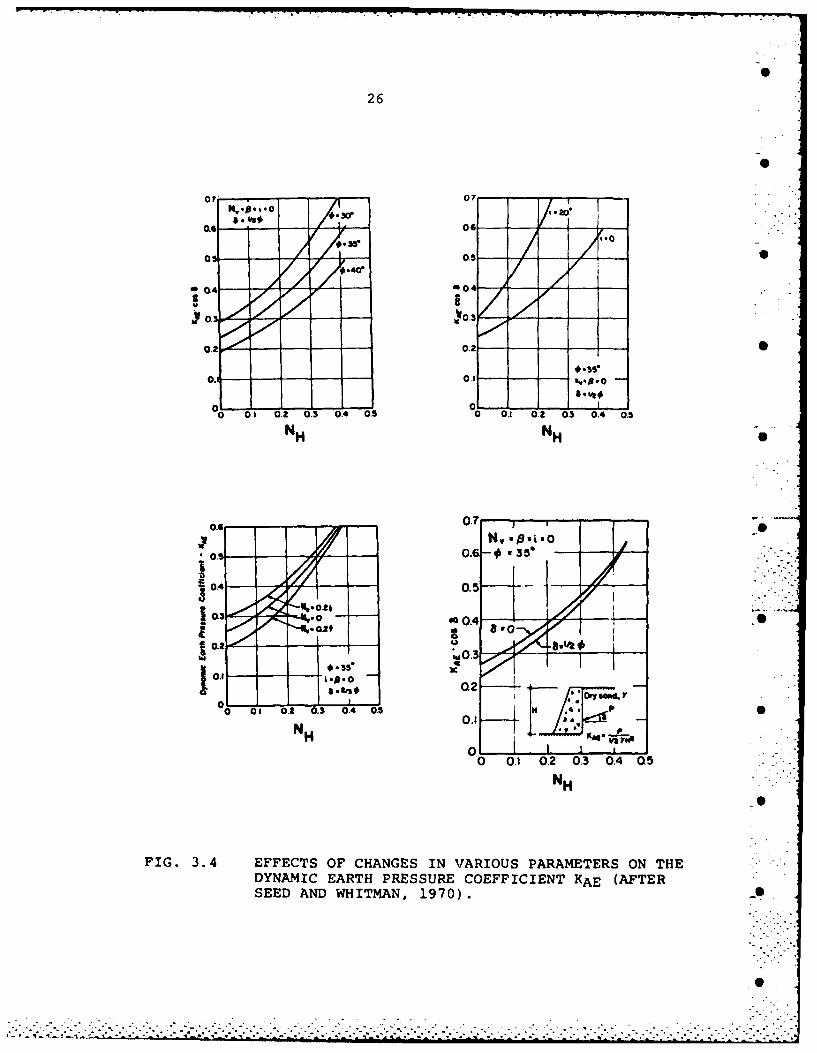
Figure 3.4 provides various charts of the quantity K orAE

KAE cos 6 plotted against the horizontal seismic coefficient NH.

KAE cos 6 represents the horizontal component of the dynamic earth .

pressure. Fig. 3.4 illustrates the sensitivity of the Mononobe-

Okabe equation to changes in the various input parameters. Based

on the observation that the inclination of the lines in Fig. 3.4 0

are all approximately at the same slope (of about 3/4) for a

relatively wide range of NH, t, and 6, Seed and Whitman (1970)

proposed a useful approximate equation for KAE:

KE K A+ (3/4 )NH (3.3)

AE A H

where KA is the static earth pressure coefficient, determined

using appropriate values of *, P, i, and 6.

"9

26

as*

0.4 - - - - - --000

.2-d -lol 0.2-

3# 3

°-' ° - - - or - /- -.

00. -..

o0 0. 0.2 0.3 0.4 0.5 0 0.30203 0.4 0.5

o.i2 03 04 os% oI 01 0 . .

NH N H

• 0- - - ._5 "-" ".0J ;0.47 1-

O0 0.5

0 0.1 -4W.2 0 0. 0

NH "-V 8.0

000 0.1 0.2 0.3 0.4 Q 5. -

N H

FIG. 3.4 EFFECTS OF CHANGES IN VARIOUS PARAMETERS ON THEDYNAMIC EARTH PRESSURE COEFFICIENT KAE (AFTERSEED AND WHITMAN, 1970).

.-.. '.

27

The location of the total thrust PAE is indeterminate from

the Mononobe-Okabe analysis. Usually, it is recommended that the

resultant force be located above the lower third point of the "-.

wall. Seed and Whitman (1970) suggest that the dynamic component

of PAE be placed at the upper third point, with the net result

being that the combined dynamic and static thrust PAE would be

located at or near mid-height of the wall.

3.2.2 Validity of Mononobe Okobe Equation

The Mononobe-Okobe equation is nothing more than Coulomb's

equation for active earth pressure, modified to incorporate a

horizontal inertia body force as well as a vertical gravitational

body force. Indeed, as discussed previously, Equation 3.2 may be

derived simply by starting from Coulomb's equation and tilting the

wall and backfill until the resultant of all body forces is

vertical (e.g. see Antia, 1982)..5

Equation 2.1 is subject to all of the same limitations as the

static Coulomb equation. Failure lines through the backfill are

assumed to be straight, which is an approximation but a good one.

Most important is the requirement that there be sufficient strain

along the assumed failure line to mobilize the full shearing

resistance of the soil in the active sense. That is to say, there

must indeed be active conditions. If the full shearing resistance

of the backfill is realized throughout the failure wedge, and if .

the horizontal inertia body force is constant within this wedge,

then the static plus dynamic stress between backfill and wall must

be distributed linearly with depth. In many cases, these may be -

'• . .. .''. ". .. "..' .. i-'.,'•: ., ".' . -"-" "- , ' " , - . " . - • ". . -' , . . ." . . . -, "- " " - - - -S

28

questionable assumptions, the deviation from which would lead to

quite different stress patterns.

Other dynamic earth pressure equations have been suggested,

usually derived on the assumption that the backfill is linearly

elastic with no limitation upon the shear stresses that can occur.

A summary of these various solutions is presented by Nadim (1982).

Not surprisingly, such equations often predict much larger dynamic

thrusts, and a different distribution of lateral stress with

depth, than an analysis based upon Coulomb's assumptions.

As described in Chapter 2, various experiments have been

performed using shaking tables with the purpose of checking upon

the validity of the Mononabe-Okabe equation. In general, the

conclusion has been that the observed total dynamic thrusts agree

reasonably well with those predicted by the theory. However, many

of these tests have not satisfied conditions that permit sliding

to occur along a failure plane through the backfill. In addition,

the dynamic thrust varies during a cycle of loading, and it is not

clear which observed value should be compared to the Mononobe-

Okabe value.

Hence it is not surprising that there are experiments showing

disagreement with theory, because of experimental conditions that

do not simulate the behavior of gravity retaining walls. On the

other hand, at least some of the reported experimental "

confirmation of the Mononobe-Okabe Equation may be only

fortuitious.

-"•' ":.. .'-•"'• -: '-'• -" :i i ' . .".''. . .. " .. . "" . " . I. .

-.--. |I I L - ., •..,

S

29

3.3 DISCUSSION OF THE SEISMIC COEFFICIENT METHOD

3.3.1 Format of Typical Seismic Coefficients

The use of a static equivalent earthquake coefficient is a

reasonable approach for the design of gravity retaining walls,

provided that neither the backfill nor the foundation soils

beneath the wall experiences a dramatic loss of strength (i.e.,

liquefaction) during earthquake shaking. A key element in this

approach is the proper selection of the seismic coefficient to use

in the Mononobe-Okabe Equation.

The seismic coefficient method is used for the design of most

civil engineering projects. Building codes and other design

manuals provide recommended values for this coefficient, which is

primarily dependent on the geographical location of the project

with respect to regions as defined by seismic zoning maps. In

most codes, the coefficient is modified by factors that are

dependent on:

* The type of foundation soil profile at the project site

* The type of the structure (e.g. buildings vs. bridges)

The natural period of the structure

* The importance of the structure (e.g. hospitals vs.

warehouses)

The last of these above factors, often referred to as the

"importance factor", is an attempt at incorporating a subjective

risk/benefit element into the seismic coefficient.

The various maps and recommendations that have been developed

are strictly for the horizontal seismic coefficients. Although -

the general Mc-nonobe-Okabe equation can accommodate both vertical

-7

..................................................................

30

and horizontal accelerations, the present lack of recommendations0

for the vertical components of acceleration prevents considering

this factor in conventional design. Also, the vertical component

of earthquake motion is generally not considered to be of as much

significance as the horizontal component.

3.3.2 Comparison of Two Seismic Coefficient Maps

Two examples of seismic coefficient maps of the United States

are shown in Figures 3.5 and 3.6. Figure 3.5 is the seismic

coefficient zoning map currently used by the U.S. Army Corps of

Engineers - USACE (1983), and Fig. 3.6 is from the tentative

building code proposed by the Applied Technology Council

(ATC-3-06, 1978). Similar maps for the United States are

published in the Uniform Building Code (UBC) and in the ANSI

regulations.

Comparison of the two maps in Figures 3.5 and 3.6 indicate

apparent differences in the delimiting of seismic zones and the

magnitudes of seismic coefficients. The ATC maps show coeffi-

cients that are double the values shown on the USACE map.

However, the USACE coefficients are intended to be applied

directly, while the ATC coefficients should be modified using

various factors as previously described. For free-standing

gravity retaining walls, the current ATC recommendation (Mayes and

Sharpe, 1981) is to use N H = 1/2 No, where N is the value of the -

seismic coefficient shown on Fig. 3.6. Thus in the final

comparison, the two maps do not conflict as significantly as at

first glance. Nevertheless, differences do exist and it should be

S " '- -' - °'-- . .' . • -• - - " - • ? • .-' .- ".- '.- b 'i . .• '.' 'L • - < - • .

31

C4,)

~~44

E- cm

I:Z.

009U

E44

32

00

E-4z

r:4

0 0

0

E-4

'14

ZrL

46

tan b 2WwN 2_ (4.5)

1 +

Once aT = Ng is obtained by solving Eqn. 4.4 or by using the

approximate solution of Eqn. 4.5, it is a simple matter to use

Eqn. 4.1 to estimate the retaining wall displacement. This

computation is illustrated in Example 4.2. 0

4.4 RICHARDS-ELMS DESIGN PROCEDURE

The design of a gravity retaining wall essentially requires 0

calculating the weight of the wall Ww, given an imposed limit for

allowable displacements. This is the inverse problem of solving

for displacements discussed in the previous section. The 0

procedure proposed by Richards and Elms is as follows:

1. Decide upon an acceptable maximum displacement dR.

2. Calculate N using Eqn. 4.1 in the form: .

N 0O 8 7 2 1/ A (4.6)= 0.08 Ag d AR . .

3. Use the Mononobe-Okabe equation (Eqn. 3.2b) to calculate

PAE" In doing so, the appropriate values of 6, 0, 6, and

i should be used.

4. Calculate the required weight of the wall using Eqn. 4.4

in the form:

-.S ••. ..

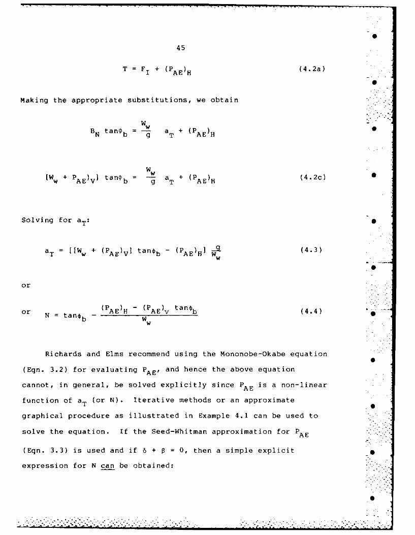
45

T FI + (PAE)H (4. 2a)

Making the appropriate substitutions, we obtain

BN tan4 b WW a + (PAE)H 0

W

BNt n b- aT

[w +AE-vI + (P AE)H (4.2c)

Solving for aT:

aT = [Ww + (PAE)V 1 tan~b- (PAE)H] W- (4.3)w

or

or (P aAE)H - v tan4 b (4.4)or N =tan ýb - SWw

Richards and Elms recommend using the Mononobe-Okabe equation

(Eqn. 3.2) for evaluating PAE' and hence the above equation

cannot, in general, be solved explicitly since PAE is a non-linear

function of aT (or N). Iterative methods or an approximateLS

graphical procedure as illustrated in Example 4.1 can be used to

solve the equation. If the Seed-Whitman approximation for PAE

(Eqn. 3.3) is used and if 6 + = 0, then a simple explicit

expression for N can be obtained:

. . . " . "

• . . . : .. . . , . . . . . . . . . . .- . .. . . . . . . -.. - . . - . . .: . .. . •

VS

44

aS

0T 7Note: oT Ng

-P. Max a =Ag

(a) Wall and Backfill Accelerations

(PAE)v

RigidBlock ~AE~H calculated using

I% T = Ng in Mononobe-Okabe Eqn.

(b) Free Body Diagram of Wall

FIG. 4. 5 IDEALIZATION OF THE RETAINING WALL PROBLEMBY RICHARDS AND ELMS (1979).

43

corresponding displacements would be 0.35 in. and 1.4 in.

Based on these results, Richards and Elms proposed an• "

alternate and very convenient equation for calculating the block

displacements d R in the medium to low range of N/A (the range of

interest in design) as:

dR = 0. 087 V2 N 41

where N and A are previously defined and V is the maximum ground

velocity. This equation is also plotted in Fig. 4.4 for

comparison with the data and with Newmark's curves.

4.3 EVALUATING RETAINING WALL DISPLACEMENTS --

Although Eqn. 4.1 is based on the results of a sliding block

model originally intended for use in predicting movements of dams -"

and embankments, it can be easily applied to predict retaining .

wall movements. The only difference in application arises from a-

slightly more complicated evaluation of the limiting acceleration -.

aT~ = Ng. For a block on a horizontal plane, N is simply equal to

tancb. However, additional vertical and horizontal earth pressure

forces, respectively denoted as (PAE)V = PAE sin (6 + •) and •"••i

(PAE)H = cos(6 + 8) and shown in Fig. 4.5, must be considered in --

the equilibrium equations for the retaining wall.

Summing forces in the horizontal direction, using the free . ".

body diagram in Fig. 4.5(b) and imposing the requirements of e

equilibrium: '-.•

S '

................................................................................................

42

- - -Various EquationsProposed byNewmark (1965)

4 - Richards - Elms2 - Equation (1979)

> AgA

-J ...................

........... .....................

(2pj-

dipUcmet (10 aa)

..............

.....................................

dslace~ N V.

0 ~2 Ag A A....

zS

0.11

0.01 0.10 1.0 10N TRANSMITTABLE BLOCK ACCELERATIONA MAXIMUM GROUND ACCELERATION

FIG. 4.4 RANGE OF NORMALIZED DISPLACEMENTS USING NEWMARKSLIDING BLOCK MODEL, AND VARIOUS EQUATIONSAPPROXIMATING THE UPPER ENVELOPE.

41

shown were obtained using several strong motion records from the 0

San Fernando earthquake. Note that there is considerable scatter

in the calculated displacement for each factor of N/A, as a result

of differing characteristics of the various earthquake records. 0

The data in Fig. 4.3 were plotted using a "standardized"

displacement scale, obtained by scaling the earthquake inputs to a

maximum acceleration Ag = 0.5g and a maximum velocity V = 30

in/sec. These same data can be replotted using a normalized

dimensionless displacement scale by dividing the calculated

displacements by V2 /Ag. Figure 4.4 shows such a plot with the 6

ranges of normalized displacements from all earthquakes used by

Franklin and Chang in their analyses. Also shown are several

expressions suggested by Newmark giving conservative estimates for

the residual displacements, each most applicable for a different . " -

range of N/A. Note that while these expressions are not true

upper bounds, they do form nearly an upper envelope for most of O-

the computed points.

To illustrate the implications of these results, the quantity

V2 /Ag typically ranges from 1 in. (for moderate earthquake with a 0

peak acceleration of 0.2g) to 4 in. (for a major earthquake with a

peak acceleration of 0.6g). In many problems of interest the

value N/A ranges from 0.3 to 0.7. At N/A = 0.3, the normalized 6

residual displacement falls in the range from 0.4 to 10.0 so that

displacements during a moderate earthquake would be from 0.4 to 10

inches, while those in a major shaking would range from 1.6 in. to

40 in. At N/A = 0.7, the upper envelope value of normalized

displacement is 0.35, so that for minor and major earthquakes, the

O

...... ..........-. .-. o".............." .... .J .-. ".". . ".............. .. . .

40

1000I00I I I I I I I Ii ~I I I I II I --

S SAN FERNANDO, CALIFORNIA EARTHQUAKE. 2/9/71

500 7_ M =6.5

SS EPICENTRAL DISTANCE 2 22.4 TO 18S Km -

34 SOIL SITES

ISCALED TO A .0.5& V 30 INJSEC

mEAN VALUE

I-ozw ,,, \U

IL

0I

z

100

S --

NONSYMMETRICAL RESISTANCE

0 1b

0.01 0.05 0.10 0 %5 5

N Transmittable Block AccelerationA Maximum Ground Acceleration

FIG. 4.3 EXAMPLE OF RESULTS USING NEWMARK SLIDING BLOCKMODEL (AFTER FRANKLIN AND CHANG, 1977).

-- I .. . . . . . . . . . . .. ,_...

39

transmitted to the block through friction forces is aT = Ng where -

the subscript 'TI denotes the transmittable horizontal or limiting

acceleration. Then the consequent acceleration experienced by the

block is shown by the dashed lines in Fig. 4.2(a).

The resulting velocity profile as a function of time can be

deduced as shown in Fig. 4.2(b). The plane's velocity increases

linearly at a slope Ag and levels off at time to, the end of the

rectangular input pulse. However, the block continues to

accelerate until its velocity catches up to the velocity of the

plane (at time t ) and this limits the time interval of them

acceleration impulse experienced by the block. The resulting

relative displacement between the block and the plane is simply

the shaded area shown in Fig. 4.2(b), i.e. the difference in the

integrals of plane and block velocities over time.

The basic concepts described above can be applied to more

complex earthquake acceleration time histories, using a relatively

simple computer program. An additional feature that must be

included is the non-symmetric resistance of friction forces, i.e.,

slip occurs only in one direction. This is consistent with the

physical behavior of retaining walls in that passive pressures are

generally more than sufficient to resist wall movements into the

backfill during earthquake shaking.

An example of the type of results obtained by Newmark (1965)

and later expanded by Franklin and Chang (1977) is shown in Fig.

4.3. This figure is a plot of standardized residual block

displacements d versus the ratio of transmittable block

acceleration to maximum ground acceleration aT/a = N/A. The data

. . .. ..

- - - E i I / - -

38

ACCELER AT ION

A Plane Acceleration

AgBlock Acceleration

NgL / ~I

to tm I iME(a)

VELOCITYPlane VelocityV Ag to

"Block Velocity

Vb Ng t

to tm TIME

(b)0

FIG. 4.2 ACCELERATION AND VELOCITY PROFILES OF BLOCK ANDPLANE SUBJECTED TO A RECTANGULAR PULSE EXCITATION.

S:: :!:

90

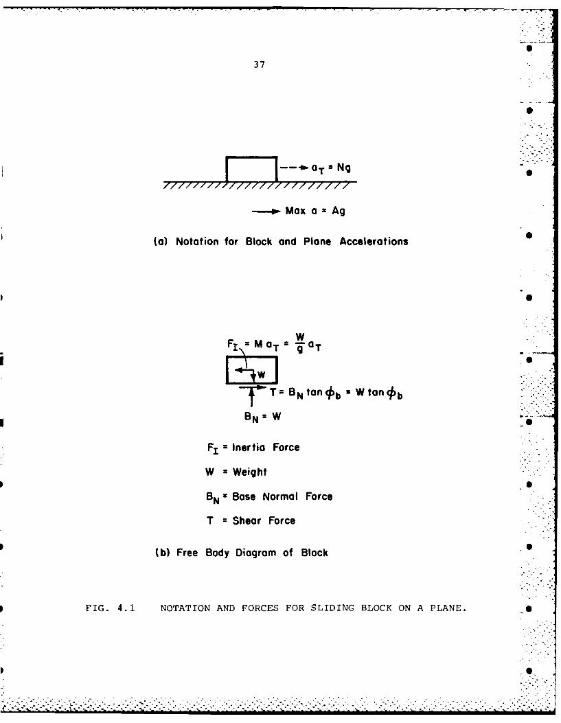
37

-- -i.OTr N g77117111111IIIIII

- Max a a Ag

(a) Notation for Block and Plane Accelerations 0

W.Fj, = Mo a g-oT

T= BN ton b W ton~b :

BN= W

F, = Inertia Force

W = Weight

BN =Base Normal Force

T = Shear Force

(b) Free Body Diagram of Block 0

FIG. 4.1 NOTATION AND FORCES FOR SLIDING BLOCK ON A PLANE. -0

. .p

-F . . . . • . . , . • • . . . : . l . _ _ . _ . • • . .. • - v. - .• . - . . . - . , . " . ,- . .

S

36

4- RICHARDS-ELMS METHOD S

4.1 GENERAL

Recognizing the shortcomings of the conventional approach for S

seismic design of gravity retaining walls, Richards and Elms

(1979) developed a design philosophy based on the concept of an

allowable permanent displacement. In the end, the design of a S

wall is still accomplished using an equivalent static seismic

coefficient, but with a more rational basis for the selection of

this coefficient. S

The key to the Richards-Elms approach is the method of

calculating the amount of residual wall movement. The approach is

similar to the method suggested by Newmark (1965) to evaluate the S

amount of slip occurring in dams and embankments during earth-

quakes. The Newmak sliding block model is discussed in the next

section, which is also intended to introduce notation and to set •

the stage for discussions of more complex models for evaluating .

retaining wall displacements.

4.2 NEWMARK'S SLIDING BLOCK MODEL

Consider the rigid block shown in Fig. 4.1 with weight W and

mass M = W/g, where g is the gravitational constant. It is •

assumed that the coefficient of friction between the block and the

plane is -P tanOb• Suppose that a rectangular earthquake

impulse (solid lines) shown in Fig. 4.2(a) is applied to the _

plane. The magnitude of the plane's acceleration a is equal to

Ag. Suppose also, that the maximum acceleration which can be

35

3.3.5 CONCLUSION ON SEISMIC COEFFICIENTSO

The conclusion that is arrived at from the above discussion

is that there are rational ways to select and use the conventional

seismic coefficient in design. However, the emphasis of design

should not concentrate on the evaluation of equilibrium of forces,

but rather on the evaluation of the retaining wall slip that

should be allowed to occur during a major earthquake. In a recent@

document issued by the USACE, it is stated that:

"... the seismic coefficient method, oftenreferred to as the pseudo-static method, is nolonger regarded as being appropriate foranalysis of embankment or foundation responsein seismic loading. Therefore its use for thispurpose should be discontinued."

(USACE, 1983)

The above statement should equally apply to gravity retaining

walls.

-S ,

O

S•.- -

-.S

-9.

.................................. ~.**.** . * ... .**- .-. *-*,.*..*"'""* ".. ...

- -. . .- -- .- - - .-. . --

tS

34

much higher than the seismic coefficient. Thus, it is recognized

that buildings designed using these recommended coefficients can

be expected to yield, should a major earthquake occur. However,

these designs are such that the yielding should not cause unaccep- -

table damage or danger of injuries and fatalities.

The implication for gravity retaining walls designed using a

seismic coefficient method is that slip of the of the wall will

likely occur during major earthquakes. This is especially true

in light of the fact that relatively low factors of safety are

usually recommended in conjunction with seismic design. The

design manual used by the Naval Facilities Engineering Command

(NAVFAC, 1982) DM-7.2 currently allows a factor of safety between

1.1 and 1.2 for seismic analysis, and for quay walls in Japan the

recommended factor of safety against sliding is 1.0 (JSCE, 1977).

Although the USACE does not have specific factor of safety guide-

lines for retaining walls (USACE, 1965), it is inferred from the

guidelines for dams (USACE, 1970) that a factor of safety of 1.0

would be acceptable in earthquake design.

An alternative to designing retaining walls using the seismic

coefficient would be to instead use the peak ground acceleration

expected for a future earthquake. However, this practice is

considered to be generally uneconomical if the inertia force of

the wall is considered in the design. It has also been suggested

that the horizontal earth pressure PAE be evaluated using the peak

ground acceleration and that the inertia of the wall be ignored.

However, this is an illogical procedure and cannot consistently

lead to sound designs.

..- .. ... ,-. .- • ... . . -, ./ .- i .3 .,•- [ .- •. •. -i ..- ....---.- . .< • . • .- - . ,, . . .. •

33

noted that for walls which are restrained from horizontal

movement, N H = 1.5 N is recommended by the ATC code.

3.3.3 Judgement in Formulation and Use

The recommended seismic coefficients in the various codes and

manuals are derived partly from theory and partly from experience

data during actual earthquakes. Considerable judgement is

necessary to formulate the zoning maps and to determine suitable

values of seismic coefficients. Thus it is not surprising that

the differences in various codes and manuals should occur, and

also that updating of the values of the seismic coefficients occur

from time to time.

It is also important to note that the intended use of the

various recommendations may significantly affect seismic

coefficient values. For example, the USACE maps were originally

* formulated primarily for use in designing earth dams, which make

up a significant part of the USACE's constructed projects. Thus,

applying the USACE coefficients to other structures should be done

* cautiously. In Japan, a similar situation exists with seismic

coefficients and maps differing for port and harbour structures,

*- roadways, buildings, etc. (JSCE, 1977).

-I

3.3.4 Seismic Coefficients and Safety Factors

Seismic coefficients typically have lower values than the

peak ground accelerations that have occurred during earthquakes.

In designing buildings, it is expected that the peak accelerations

(due to amplification of ground motion in the structure) could be

I

I I

47

(PAE)H - (PAE)V tan bw (4.7)w tan~b - N

5. Apply a factor of safety of 1.5 to the wall weight

RWw.

A design problem, using the above procedure, is illustrated in s

Example 4.3.

4.5 COMMENTS ON THE RICHARDS-ELMS METHOD

The Richards-Elms procedure is rational and simple to apply.

It is, in effect, a counterpart of a procedure used for buildings

(Newmark and Hall, 1982) where the ratio of design seismic

coefficient is chosen on the bas~s of the ductility ratio (of

*. expected strain to yield strain) that a structure possesses before

there is extreme structural damage or danger of collapse. Its "

major disadvantages are that it does not consider certain

* kinematic restrictions upon retaining wall behavior, the

deformability of the backfill or possible tilting, and the

statistical variability of earthquake ground motions. In a

fashion, these factors have been taken into account in the factor

of safety of 1.5 on the wall weight, which is somewhat 4

conse-vative compared to usual values of recommended safety

* factors ranging from 1.0 to 1.2, as discussed in Section 3.3.

However, it is not clear that there is a rational basis for the -4

suggested safety factor of 1.5 on wall weight.

"2 ,' .

.. . . .. .. ° -**. .. .*. * .. " .*

|0

48

The remainder of this report will consider some of the

deficiencies in the Richards-Elms procedure, and will suggest

improvements and corrections, while retaining the essential

simplicity and soundness of the basic approach.

0 ,°.

0 °J'.

- •

0-

° ". .. . . . . . . . . . . . . . . . . . . . . . . ..,o " o '.°" 2 " .J . .. °.

49

EXAMPLE 4.1

Given: Retaining wall and backfill with properties shownin Figure E4.1.

Find: The maximum transmittable acceleration N, using theRichards-Elms method.

Solution: The weight of wall Ww is calculated to be 32.81 K/ft.From Eq. 3.2a, PAE= (1/2)(0.120) (25) 2 KE = 37. 5 KAE K/ft.Assuming values of N, values for P and KAE arecalculated from Eqs. 3.1 and 3.2b. A new value ofN is then computed from Eq. 4.4. Results of thesecomputations appear in Table E4.1 and are graphedin Fig. E4.2. The answer is given by the intersectionof a curve through the computed points and a linethrough the origin at 450.

.0

-* -2.5' Bockfill Slope i =0

2.54.

440

Bockfill PropertiesH 25' . ,. zo= 300 '•

' q4 C =0tE120 PCF . .

=C- 150 PCF-

-

V 4 .% ,.

'. 15' 0-.0

FIG. E4.1

. .

50EXAMPLE 4.1 (continued)

Table E4.1

AS SUMED (KAE) COMPUTEDN 'P H N

0.05 2.860 0.364 0.161

0.10 5.710 0.397 0.123

0.15 8.570 0.433 0.082

0.20 11.310 0.473 0.036

0.3-

SOLUTIONz0.2 N 0.I12

o0.2-a.

80.1Data fromCalculationsTable E4.1

0 0.1 0.2 0.3ASSUMED N

FIGURE E4.2

For comparison, N is also computed using Eq. 4.5, yielding

N = 0.106

- - ... . ......... ....

51

EXAMPLE 4.2

Given: The wall in Example 4.1.

Find: The permanent displacement caused by an earthquakecharacterized by A = 0.3 g's and V = 15 in/s, - -

using the Richards-Elms approach.

Solution: From Eq. 4.1:

dR = 0.087 0.3'386 -0.112

= 0.087 (1.94) (51.48)

= 8.7 in.

EXAMPLE 4.3

Given: The backfill and frictional resistance propertiesin Example 4.1.

Find: For a wall 25 feet high, the required weight of wallif an earthquake with A = 0.3 g's and V = 15 in/sis to cause a permanent displacement of 1 inch, ac-cording to the Richards-Elms approach.

Solution:

Step 1 - d = 1 inch

Step 2 - From Eq. 4.6, N = 0.192

Step 3 - Eq. 3.1 gives 1 = 10.890

- Eq. 3.2b yields KAE = 0.467

- Eq. 3.2a gives P = 17.51 K/ft.AE

Step 4 - From Eq. 4.7, W = 45.44 K/ft.

Step 5 - Applying a safety factor of 1.5 to computedWw: •

Required weight of wall = 68.2 K/ft.

-0<

O

52

5-KINEMATIC CONSTRAINTS UPON MOTION OF BACKFILL S

5.1 THE TWO BLOCK MODEL -- ' "

In the Richards-Elms model, the retaining wall is modelled as

a single sliding block on a plane, when in fact the actual

behavior is much more complex. A more realistic model is the

two-block model developed by Zarrabi (1979), which is shown •

schematically in Fig. 5.1. In this model the wall is represented

as a block on a horizontal plane, and the wedge of soil (behind

the wall) that "fails" during sliding is represented by another O

rigid block on an inclined plane.

The kinematic constraints on the two-block model are that .

during sliding, contact force and acceleration continuity must be

maintained between the two blocks themselves, and between each of

the blocks and their respective sliding planes. This gives rise

to three equations of acceleration continuity that must be

satisfied simultaneously with the equations of equilibrium. " .

The most significant constraint in terms of the mechanics of

the problem is that of maintaining contact between the sliding

soil wedge and the inclined plane. For outward movement of the

wall to occur, there must be a simultaneous outward and downward

movement of the soil wedge. Thus, even when there is no vertical •

ground acceleration, the backfill wedge would still experience

vertical accelerations.

. . - • .

-- • .l i

53

Kinematically constrained 5directions of relative slip

// ilure Plane

7 •-.- Ground Acceleration

(a) Actual Physical Situation

Rigid Sliding

Plastic deformations

Interaction of blocks necessary for movement Care ignored

through active force PAE

(b) Two Block Model Idealization by Zorrobi o

FIG. 5.1 SCHEMATIC OF IDEALIZATION OF RETAINING WALL S.PROBLEM BY ZARRABI (1979).

-. . . .-- • ..- .. . , . , ..- .. - .. .. .- . . . . . . .. . . .. : -- : .:

| | •

° ..54 ..:

5.2 COMPARISON WITH SINGLE-BLOCK MODEL •

Vertical accelerations in the backfill wedge affect the '.. ----.

active earth pressure PAE between the wall and the soil• This is .-.- -. :,-• • . . -...

reflected by the • term and the factor (I-Nv) in the Mononobe •

Equation (Eqn. 3.2). It can be she::,,n that for continuity of

acceleration normal to the failure plane at any instant in time, .i -

the following equation must hold: •

Nv(t) = Av(t) + [AH(t) - NH(t)I tan [@(t)] (5.l-a)

or . •

NH(t) = AN(t) + [Av(t) -My(t)] cot [@(t)] (5 2-b) " ./ •°'" / •

where AH(t) is the horizontal ground acceleration coefficient. : •

Av(t) is the vertical ground acceleration coefficient ""'"'"'"NHIt) is the transmittable horizontal acceleration.i22•2•2211?'".'.'-.'-

coefficient of the wall and soil wedge. ",.:•;..•,:•w•

Nvlt) is the transmittable vertical acceleration coefficient [ ..•:.of the soil wedge.

-•-?i-i':< i<.-'.81t) is the angle of inclination of the failure plane with "-.'-"-"-.',

respect to horizontal (see Figure 5.1). "•' "'"'""

The notation It) indicates the above quantities to be variable " .... :-•

S. .- ,with time• Thus, the transmittable acceleration at any instant in ?.i-.-

time is dependent upon the ground acceleration at the same time.

This is in sharp contrast to the single-block model proposed by

Richards and Elms where the transmittable acceleration is constant '"'"--•"•"J ,-° J• °° ,0

with time. .... ."

A schematic comparison of the sliding processes of the 121?.•i.i.."

Zarrabi (two-block) and Richards-Elms (single-block) models is ?['•'.i[•[i•[[

shown in Fig. 5.2• In the two-block model there is a threshold. "--"-"-

7-

•"?--"-'?-."?':. • • ,•."-.'--A ?--?--?-:..':--?--..,,.,,,,•..• ,• .,_-. -. ' --. -" -'-" . -- : --.•, .,,...• , ,.. ,.•,,. • ,•.,-v.-.--..-.-.-.-.-..'...:. ..... . . . . ... ..-..-.. v...v.-...:.-..-..-i.. ... . . : i. .. .... ... . .?.-i .-•--.>-i.i. .- .- . . .. . :- ...-..-,

55

-Ground

Richards - Elms(Single Block) Model

-.- Zorrabi (Two-Block) 0z model

2 N M

uJ NI

I. TIME

oe'

TIME

I- 0z

w~ > W 00>I00

TIME

FIG. 5.2 SCHEMATIC COMPARISON OF SLIDING PROCESSES OFTHE RICHARD-ELMS (R-E) AND ZARRABI MODELS.

--. !

56

acceleration NT required to initiate slip. Provided that S

comparable assumptions are made concerning the properties of the

backfill, the value of NT is exactly the same as the value of N

used for the Richards-Elms procedure. However, after initiation 0

of slip, the limiting acceleration NH at any time during a cycle

of slip can be greater or less than NTg.

As a result, the active thrust P is also changing during SAE

sliding. An illustration of how this physically occurs is shown

in Fig. 5.3 for the case where there is no vertical ground

acceleration (AV =0). When the ground acceleration AHg exceeds 5

the transmittable acceleration NHg [Fig. 5.3(a)], the vertical

backfill wedge acceleration Nvg is in the downward direction.

Hence, the inertia force is in the opposite upward direction, 70

effectively causing a decrease in the weight of the soil and a

subsequent decrease in PAE" The reverse occurs during the later

stages of slip when A Hg < NHg as shown in Fig. 5.3(b) 0

The equations applicable to the evaluation of residual slip

in the two-block model was developed by Zarrabi (1979). The

solution procedure for these equations is fairly complicated in S

that during slip, the value of N H must be evaluated at every

time-step. Also, since e is a function of N H and NV, the solution

for NH must be obtained iteratively. Wong (1982) subsequently

developed a more efficient scheme, in which part of the solution

to the governing equations is precomputed and stored in computer

memory, thus requiring fewer iterations. Alternatively, it might 9

be assumed that 0 remains fixed in which case the Mononabe-Okabe

equation no longer applies and the basic equations for dynamic

S

57

r 0

00U) 1-4

(n E-4

U)U

>w w hz 0..Zh.r

E 0 0

zz x \rUý

z

(0 -j

o'x E-424 z z

A0 0

"wlo

+ 0- in;in

+

C ~44CIO.

58

equilibrium and continuity are solved simultaneously at each time

step.

There is one other feature of Zarrabi's two-block model that

deserves mention at this point. This is the implicit non-

symmetrical resistance of two-block model, so that unlike the

Richards-Elms/Newmark model, no explicit assumptions regarding the

non-symmetrical nature of the sliding block resistance are

necessary.

5.3 NUMERICAL RESULTS

The net result of the kinematic constraints in the two-block

model is that the calculated residual displacements are smaller

than those using the single-block model. This is illustrated in

Fig. 5.4, which shows the ratio R2 / 1 plotted against N/A (for the

single-block model) or NT/A (for the two-block model), where R2 / 1

is defined as:

R dR Residual displacement of two-block model2/1 d R Residual displacement of single-block model

Note also that the values of A, N and NT, as used here, are not

functions of time, but are constants depending on the earthquake

record or the wall/backfill properties.

The results shown in Fig. 5.4 are based on limited results

using the average values of residual displacement calculated using

four earthquakes (Antia, 1982). The unit weight of the soil, the

wall height and the height of the wall are properties that can be

collectively described by the value of NT. However, the soil and

S - l .•' '. . / . ".-.-'-• . - . .i i . ]• .. i i. -, • - . - • •-• i- i .•..5.• ¢ -• .

- -- - - - - -- -

59

0C

(0

coz nfl .0 Z E-

i 012. 0 cn

Lii0 m

0I 00

00 E

4 E

w z

.~ 0tt

00

z-7 0 LAo 0

~~01- 40 I) l

_ uc

.LN3VV43DV-dSIOI 1300Vd MOO19 3-19NISJ.N3bVGOV-dSla -13GOVI A30-Oi9 m P4..

.........

60

backfill properties cannot be as easily incorporated in a single

parameter,and the results shown in Fig. 5.4 are only for a typical

case which might be encountered in practice ( = = 300; 6 = i =

= 0). 5

It is seen from Fig. 5.4 that the differences between the two

models (smallest R2/ 1 ) are greatest for small values of N/A and/or

for small values of A. An explanation for this trend is that as S

either N or A increases, the angle of the failure plane 0(t)

becomes generally smaller (flatter). Hence, Nv (t) which is

directly related to tan [G(t)] becomes smaller (Eqn. 5.1-a), so O

that the vertical acceleration and its effects are reduced. In

the limit, as A or N becomes large (roughly corresponding to T

becoming large), the angle e(t) would be nearly zero (horizontal),

and hence no vertical backfill motions would result from purely

horizontal ground motions.

The reason for the ratio R2 / 1 being consistently less than

one is not completely clear at the present. It would be not

unreasonable to envision that although NH(t) and hence PAE vary

with time during slip, that on the average, the results of the S

two-block model should be same as the single-block model.

Intuitively, however, the mere fact of adding "constraints" to a

model implies a restriction of otherwise freer motions. Another

intuitive notion, from a work-energy viewpoint, is that the

two-block model has more energy-dissipating mechanisms than the

single-block model. Whereas in the single-block model, the O

earthquake energy causing motion can only be dissipated through

friction forces at the base of the wall, the two-block model has

• -. -•- -. • - .. . .-.- . .- --. -. . -. - -. . . . . . ...-. , -- , - ..-- -- -.-.--. --.

74

rhe goodness of fit is shown in Fig. 6.3; for N/A between 0.1 and

3.7, the value predicted by this equation is within 10% of the

-omputed C1 (within 5% for N/A > 0.4). This expression does not,Re

as it ideally should, go to zero as N/A approaches unity although

it predicts insignificant values in that range.

The scatter of the record means dRo is indicated by the

coefficients of variation in the second line of Table 6.1, which

are statistics for the random variable Fs Ro /Z . For inter-

mediate values of N/A, the uncertainty from record to record is

about the same as for differently oriented walls during any one

shaking. At larger N/A, the orientation effect has much greater

uncertainty.

Again, all these results were developed using only the

horizontal components of recorded ground motions.

6.5 EFFECT OF VERTICAL ACCELFRATIONS

Downward acceleration of the plane supporting a block will

decrease the normal force at the interface, thus decreasing the

transmittable acceleration and increasing the tendency to slip.

Conversely, upward acceleration increases resistance to slip. In

a ground motion with many peaks of acceleration causing slip, the

effects of the vertical component of ground motion may be expected

to cancel. Hence the vertical component of ground motion has

generally been ignored when computing sliding block displacements.

The actual effect of vertical ground accelerations has been

studied using the suite of 14 earthquake records described above.

For each computation, the vertical component of acceleration wasS

.............................................................

73

100

50 _ __ _

Mean Value Curve from Fig. 4.3

5

dRe

0.5

0

0.01 0.05 0.1 0.5 1.0 5I

N/A

FIG. 6.2 MEAN DISPLACEMENTS FROM THIS STUDY COMPARED 0WITH THOSE FROM FRANKLIN AND CHANG (1977).

9ii.i

72

eynonential with a spike at the origin. For N/A of 0.4 and 0.5, 0

it ii somewhat similar to a log-normal distribution.

A'I of these results were computed using only the horizontal

components of the recorded ground motions. 0

6.4 SCATTER AMONG DIFFERFNT SITES AND EVENTS

The next step was to examine the record means d Ro For each

selected N/A, each of these fourteen values was first normalized

to a common peak acceleration and peak velocity using V2/Ag

scaling. (As previously discussed, A is the largest absolute

acceleration from both components of a record, and V is the peak

absolute velocity from the component containing that accelera-

tion.) Then the 14 normalized values of Ro were averaged to

obtain the overall mean displacement dre; that is:

dRe = Ave [aRe] (6.1)

The scatter of the record means about the overall means was also

analyzed.

The overall mean displacements, in normalized form, are

plotted as a function of N/A in Fig. 6.2. As a result of the

scaling scheme used in Wong's analysis, these results fall below

the average curve from Fig. 4.3. A simple expression which

provides an approximate fit to the mean slips is:

237V -9.4N/ARe Ag (6.2)

.. . .. ..-.. .-.. - . .- . . . . .. , . . , . . . . . . .. . . . . . . . "

71

Table 6.1

COEFFICIENTS OF VARIATION ARISING FROMUNCERTAIN ASPECTS OF GROUND MOTION

COMPONENT N/AOF - -

UNCERTAINTY 0.1 0.2 0.3 0.4 0.5 0.6 0.7 0

ORIENTATIONOF WALL AT 0.32 0.42 0.51 0.64 0.86 1.12 1.30

A SITE

EARTHQUAKETO 0.53 0.54 0.58 0.58 0.56 0.50 0.41

EARTHQUAKE

A

z 0.2 ... <0.05 0.05 0.07 0.15 0.120.3 <0.05 0.07 0.13 0.22 0.27

0.4 <0.05 <0.05 0.05 0.10 0.18 0.30 0.370.5 0.06 0.12 0.25 0.37 0.57

u 0.6 0.07 0.15 0.33 0.44 0.66

0.7 0.08 0.19 0.42 0.51 0.73

S

. .- .. .

70

6.3 ORIENTATION EFFECTS

For a complete analysis of this effect, it would be desirable

to compute, from the two observed components of each record, the

time histories of motions in many directions. However, only the

two recorded components have been used in this study to evaluate

four possible permanent displacements.

Four values of permanent slip dRe were computed from each of

the 14 records for values of N/A from 0.2 to 0.7, with no

normalization of the records and ignoring vertical accelerations.

For each of the records, an average aRo was determined (used for

the analysis in Section 6.4), plus four values of the ratio E0 =

d /a Thus for each N/A, 56 values of F 0 were obtained. The

mean of E is, by definition, unity. The coefficients of0

variation are listed on the first line of Table 6.1.

It may be seen that the scatter in the ratio E increases as0 -

N/A increases. This occurs because, at the larger N/A, one or

more component-directions may not cause any permanent slip. For

example, at N/A = 0.7 the 1940 El Centro record causes no slip in

the east-west direction, and very little for a wall oriented so

that it can slip to the south. Overall, of the 56 computed slips,

17 are zero for N/A 0.7, eight are zero for N/A = 0.6, and 2 are

zero for N/A = 0.5. Numerous other values are so small as to be

essentially zero.

Because of the tendency for an increasinq number of zero

values as N/A increases, the distribution of E0 changes as N/A

changes. For N/A = 0.1, the distribution was found to be

approximately normal. For N/A = 0.7, it is more nearly . .

............ ........

69

N E-

g0-0.-25g0.2g•'V" ''-- -"vVYo-:669:

-- 0.3gSW

(a) Example N-S and E-W Components of an Earthquake

0.5

0/.2g

O0.2g

/E 0 0 .3g

s E°

0. 15 g "

b ifrn rett o R i W25ga...... ....

"0,,.2g .20/.3g • E- ,

Earthquake Components

FIG. 6.1 EFFECTS OF RETAINING WALL ORIENTATION.

. . . . . • .

68

tions are different in the positive and negative sense of each

component.

An important implication is that the permanent slip

experienced by a retaining wall during an earthquake will depend S

upon the orientation of the wall. For example, the four retaining

walls shown in Fig. 6.1 would be expected to experience differing

amounts of permanent displacement during any one earthquake. 0

Indeed, some walls might have permanent displacement while the

others would not yield at all. This is an important aspect of

uncertainty in the prediction of the motion which may be O

experienced by any particular wall.

In previous work, it has been usual practice to normalize a

component of a record to the maximum acceleration and velocity in 0

that component. However, this procedure tends to obscure the

orientation effect just described. In the study by Wong, one

acceleration - the largest absolute acceleration from either of O

the components - was used to normalize both components. This was

done because the earthquake motion recorded at a site is always .

characterized by this largest absolute acceleration, and this

number would always be used when judging whether or not a wall (or

any ether structure) located at the site lived up to expectations.

The choice of a velocity to characterize the ground motions •

at a site is less obvious. For this study, use has been made of

the largest absolute velocity in the component containing the

largest peak acceleration. This choice is consistent with past

practice and should lead to the least confusion concerning

interpretation of results.

O

67

characterized by having peak accelerations greater than 0.15 g

resulting from earthquakes with magnitudes between 6.3 and 7.7.

(Actually, all but 2 records are for magnitudes between 6.3 and

6.7). The restriction on peak acceleration was imposed so that

all records would be typical of those which might cause signifi-

cant displacement of actual retaining walls, and distortion would

not be introduced by scaling of weak motions. The limitation upon

magnitude was used to narrow the range of durations of earthquake

shaking, which roughly correlates with magnitude. Ideally a

similar study should be performed using other sets of records

corresponding to smaller and larger magnitudes, but as yet this

has not been done.

Analysis of scatter in sliding arising from differences in S

ground motions has been divided into three parts. First there are

the differences in sliding associated with the several components

of motion at one location during one earthquake. Second there

are the differences from site to site and earthquake to earth-

quake. Finally there is the effect of the vertical component of

ground motion. In the end, the influences of these three effects

will be lumped together. However, considering them separately

will provide an understanding of the relative importance of the

several effects. O

6.2 SCALING OF RECORDS

A typical ground motion record has two horizontal components.

As a matter of course, the peak accelerations (and velocities) are

different for the two components. Moreover, the peak accelera-

. . .*. .-

66

6 - RANDOM NATUPE OF GROUND MOTIONS

6.1 INTRODUCTION

This is the first of three chapters dealing with uncertainty

in the prediction of the residual displacement for a gravity

retaining wall. As discussed in the introduction, such uncer-

tainty arises because of differences in the details of ground

motions, because of doubts as to the actual resistance of a wall

to sliding, and because of errors in the models used to predict

residual displacement for a given ground motion and given

resistance parameters.

This chapter deals with the consequences of the essentially

random nature of ground motions. As discussed in connection with

Fig. 4.3, different ground motions each normalized to the same

peak acceleration and velocity can produce quite different amounts

of sliding for the same N/A. These differences are associated

with differing frequency contents, differing distributions of -

peaks and differing directions of shaking. Because the prediction

procedure ultimately recommended in this report uses the simple

sliding block model, these various effects are studied using that

model. Thus the results potentially apply to all problems for

which the sliding block model provides a reasonable prediction of0

permanent displacement or deformation including certain earth

slope movements in earthquakes as well as retaining walls.

The analysis here uses results from a study of the mean and

distribution of sliding caused by a suite of normalized ground

motion records (Wong, 1982). This study utilized a relatively

small set of records - 14 in number and listed in Appendix A -

S -, - .

65

5.5 SUMMARY S

The use of a single-block model analogy by Richards and Elms -

(1979) tends to overestimate the residual slip of a retaining wall

due to earthquake shaking. Zarrabi's model, using the concept of

two interacting blocks, provides a better estimate of the actual

slip, as confirmed by model tests on a shaking table.

An important issue mentioned briefly in this chapter involves 0

whether it is valid to assume a failure plane inclination 0 which

varies with the instantaneous ground acceleration. This and other

issues regarding how changes in other parameters (i, *b' i, • and

6) affect the results, are treated in Chapter 8.

/- S-.

S" .o .-

,S

• -S

-. . . . . . . . . .. . . . . . . . . . . . . . . . . . . . . . . .

64

0.40

Measured (Ground)U, Measured

0.20-(al

~¶R-E0-

100

0-0.20-

-040

0.10S

0.1

2 SE

E 6-

Co

/Zarrobi

M-`teasuredy

0 0.08 0.16 0.24 0.32 0.40 0.48 0.56 0.64TIME in seconds

FIG. 5.6 COMPARISON OF RICHARDS-ELMS (R-E) AND ZARRABISLIDING BLOCK MODELS WITH EXPERIMENTAL RESULTS(FROM JACOBSEN, 1980) (SEE CHAPTER 2 FOR DETAILSOF EXPERIMENTS, WHICH WERE PERFORMED BY LAI, 1979).

63

experimental results obtained by Lai (1979). These experiments 6

were previously described in Chapter 2.

A typical comparison of theory and experiment is shown in

Fig. 5.6. As can be seen, the Zarrabi two-block model is a better 0

simulation of the time histories of acceleration, velocity, and

relative displacement. Clearly, the limiting acceleration is not

constant as predicted by the single block model. Also noted by 5

Jacobsen was the fact that the two-block model predictions are in

better agreement during the beginning of the shaking as compared

to the latter part of the shaking. It is conjectured that this is

in part due to the physical constraint that the toe of the soil

block has to undergo some plastic deformation in order to slide

with the wall. The rigid two-block model inherently assumed this •

effect to be negligible.

An important point with regard to the comparisons made by

Jacobsen, is that the calculations he performed should be

recognized as "Class C" predictions, i.e. predictions after the

fact. In particular, Jacobsen used the angle of inclination 6 of

the failure plane obtained from the experimental results as input S

to the computuer simulation models. As opposed to Zarrabi's

procedure where 8 varied with acceleration, Jacobsen chose instead

to use a fixed 0 (measured in the model) and found that this gave

better agreement with the experimental results.

_0

0 "-

62

E-4

z E

00

1 u0 zci 00

0 c

d0 w0 E- 0

0

-E-

00

0z 005 0

0~ 0E

4 04 z

0 5:4

N 0 0D

ci 0

IS

S

61

at least an additional frictional energy dissipation surface

through the failure plane in the backfill. Though these

explanations are intuitively plausible, they would need to be

justified rigorously by further research.

Another important observation from the results shown in Fig.

5.4 is that it is not possible to normalize the residual

displacements of the two-block model by dividing by V2 /Ag as was

the case for the single-block model. If it were possible, then

R R dR/(V2/AG) (2/1 R dR/(V /Ag)

should only be a function of N/A or NT/A. Since it is known that

dR/(V 2 /Ag) is only a function of N/A (see Section 2.4), but that

R2/1 depends on A, it can only be concluded that dR/(V 2 /Ag) is not

* solely a function of N/A, and hence cannot be normalized.

However, as a practical matter in design considerations, the

"results of Fig. 5.4 can be replotted as shown in Fig. 5.5, where

the horizontal axis has values of N or NT instead of N/A or NT/A.

This scheme condenses the values of R2 / 1 to a narrower band of

data, minimizing the influence of A. Wong (1982) has suggested

that R can be approximated for design purposes as solely a2/1

function of N.

_ 5.4 COMPARISON WITH EXPERIMENTAL RESULTS

Jacobsen (1980) performed a detailed comparison of the

Richards-Elms single-block and Zarrabi two-block models with

"~~~~~~~~~~~.'-. "-.'''•"- -• . ...... .i.•.• . -.-. ."'- ..... .... ............ ,....:.....,,....,.........o... .... :........,...... ,M :. ,,,

B * - .. 75

00

0 CD

ga~ 00

le 0

00 z2z

a.W 0D0z

E40

E-40

aZ4

CY H cf

0~~ 00 *

B00 0ll

76

scaled in the same ratio as the horizontal component. The S

influence of the vertical accelerations is indicated by the ratio

Ev = dR/dR where d is the slip computed when vertical -..

accelerations are considered. The ratio E was found to depend •

upon the strength of the input acceleration (the coefficient A) as

well as upon N/A. For each pair of values for A and N/A, up to 56

values of E were computed (less those cases where d = 0 and Sv Re

cases where dRe is so small that division by it would give a value

of E which might be much in error). Average values are plottedV

in Fig. 6.4, and coefficients of variation are listed in the lower S

portion of Table 6.1.

Figure 6.4 indicates that, on the average, incorporating . -

vertical ground accelerations causes greater residual displace- .

ments. This can be understood by considering a hypothetical case

in which upward and downward accelerations both reach peak values

of 1.0g. When the peak downward acceleration occurs, resistance S

to slip disappears entirely, whereas at the peak upward

acceleration the resistance is merely double that for zero

vertical acceleration. Clearly, the potential effect of downward S

acceleration on slip is greater than the influence of upward

acceleration.

The coefficient of variation for the function E is small -v

except when both A and N/A are large. As would be expected, with

large N/A there are fewer intervals during which slip occurs, and

hence the sense of the vertical acceleration in these moments is S

quite important. The influence of vertical accelerations would

. .- . .

. . . . . . . . . . . . . .~ ~ ~ ~ . . . . . . . . . . . . .

". . . . . . . . . . . . . . . . . . . ..''.. - * ."."-.-' -", "' "''" ' -' .- .".', . . . ''- -. . '. -... -. . .. -. -"'",''. ''..'..

77

1.5 -

1.4- A0.0

1.30.5

IL1.2 0_ _ _

w0.

w0 .

0-0 0.i 0.2 0.3 0.4 0.5 0.66 0.7

N/A

FIG. 6.4 EFFECT OF VERTICAL GROUND ACCELERATION ONRESIDUAL DISPLACEMENT OF BLOCK.

78

appear even greater if cases in which dRe = 0 but dRy P 0 were

included.

Wong suggested an equation for the average effect of vertical

accelerations:

= 1.015 - 0.2N/A + 0.72(N/A) 2 (6.3)

vS

which is valid for 0.2 < A < 0.7 and 0.1 < N/A< 0.7. "Average" in

this sense implies averaging over a range of values of A as well

as over a set of computed slips.

6.6 COMBINED UNCERTAINTY

One way to estimate the overall uncertainty arising from the

combined effect of orientation of the wall, site-to-site and

event-to-event differences, and vertical ground accelerations is

to combine the coefficients of variation in Table 6.1. We woulO-

estimate the slip of a block as:

dRv =o EosEv Re (6.4)

where d is a deterministic function of N/A (as given in Fq. 6.2)Re

and Eo, Es, Ev are random variables which depend upon A and N/A.

If we further assume that Eo, F and F are independent, then the

coefficient of variation VR of dRv is:

2 ( + )(1 + V2 )(1 + V) - (6.5)

. . . ..

79

where Vo, Vs and V are the coefficients of variation of E , E-

and E respectively. The resulting values of VR are tabulated inv R

Table 6.2. As would be expected from comparison of the individual

V0 , Vs and Vv, vertical ground accelerations contribute relatively 0

little to the overall uncertainty except at large values of N/A.

Even here the predominant uncertainty comes from the unknown

orientation of a wall relative to the principal axes of the ground 0

motion.

Alternatively, values of VR may be determined directly from

the 56 computed values of residual slip for each A and N/A. These 6

results are given in Table 6.3. Comparing Tables 6.2 and 6.3, it

is seen that the directly-evaluated VR (Table 6.3) are always less

than those (Table 6.2) computed by assuming that the three effects

discussed in Sections 6.3, 6.4, and 6.5 are independent. Clearly

some degree of correlation actually exists among these effects.

From the results at small N/A, it may be deduced that the O

orientation and site-to-site effects are correlated to a slight

degree. At large N/A the VR do not increase significantly as ARO

becomes larger, implying that the effect of vertical ground

acceleration is strongly correlated to one or both of the other

two effects. This latter conclusion seems reasonable: vertical

accelerations are important only when there are a very few spikes 0

of horizontal acceleration that cause slip, and having only a few

such spikes can also lead to a strong orientation effect.

For design considerations only the results in Table 6.3 are

of interest. However, having looked at the various effects .

................... . .. . .. .

"-•" •'~~~~~~~~~~~~~~ ~~~.. .•'..'-..i .. ..........-,........ i..i-L . .I'•-.. -....-. ?.,...-.,..-., .-.--.

00

80

Table 6.2

OVERALL COEFFICIENT OF VARIATIONASSOCIATED WITH UNCERTAIN NATUREOF GROUND MOTION, BY COMBINING

UNCERTAINTIES IN CONTRIBUTING EFFECTS

N/A

0.1 0.2 0.3 0.4 0.5 0.6 0.7

0.2 0.64 0.72 0.83 0.94 1.14 1.37 1.48

0.3 0.64 0.72 0.83 0.94 1.15 1.40 1.54

0.4 0.64 0.72 0.83 0.95 1.17 1.44 1.60

0.5 0.64 0.72 0.83 0.95 1.19 1.48 1.78 -

0.6 0.64 0.72 0.83 0.96 1.24 1.54 1.87

0.7 0.64 0.72 0.83 0.98 1.30 1.60 1.95 -

0

. . . . .. . . . . . . . . . .

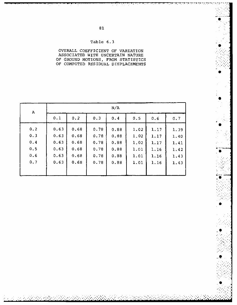
81

Table 6.3

OVERALL COEFFICIENT OF VARIATIONASSOCIATED WITH UNCERTAIN NATURE

OF GROUND MOTIONS, FROM STATISTICSOF COMPUTED RESIDUAL DISPLACEMENTS

N/AA

0.1 0.2 0.3 0.4 0.5 0.6 0.7S

0.2 0.63 0.68 0.78 0.88 1.02 1.17 1.39

0.3 0.63 0.68 0.78 0.88 1.02 1.17 1.40

0.4 0.63 0.68 0.78 0.88 1.02 1.17 1.41

0.5 0.63 0.68 0.78 0.88 1.01 1.16 1.42

0.6 0.63 0.68 0.78 0.88 1.01 1.16 1.43

0.7 0.63 0.68 0.78 0.88 1.01 1.16 1.43

Ao

. . . . . . . . .. . . . . . . . . . . . . . . . . . . . . . .

. . . . . . .. . . . . . . . . . . . . . . . . . . . . . . . .

82

separately has been of considerable value in understanding the

importance of the several contributions to overall uncertainty.

6.7 PREDICTING RESIDUAL DISPLACEMENTS 6

If the effects of vertical ground acceleration are ignored,

Eq. 6.2 provides a good prediction for the average residual

displacement for a given A, V and N/A. There is a small "fitting 0

error" and there is still some statistical uncertainty in the

determination of the actual mean displacement owing to the limited

size of the suite of earthquakes used in the calculation. 0

However, these uncertainties are small compared to the scatter in

residual displacement resulting from the random nature of ground

motions. When vertical accelerations are introduced,Eq. 6.2 may

be modified to:

1Rv vaRe (6.6)

where v is given by Eq. 6.3. As discussed in Section 6.5, E isV

actually also a function of A, but the error introduced by using 0

Eq. 6.3 is small compared to the scatter associated with

orientation and event-to-event effects. -

Table 6.3 provides estimates of the coefficient of variation

of the residual displacements. If the distribution function for

the displacements is known or assumed, Eq. 6.6 plus Table 6.3

provide a basis for estimating probability that various levels of

ground motion might be exceeded. Since to some degree the

uncertainty in d arises from a multiplication of the three .

.... . .. . ...... .-. _,•.._.,.?": -•.i,:.:.L%.._• "..~. .-'-• , --. ••• -•.iLii..-.. .. .. ... : .-?i .i...:,>...:...i-:-•L•:......... •.. - --- '.?....-*,,:?-

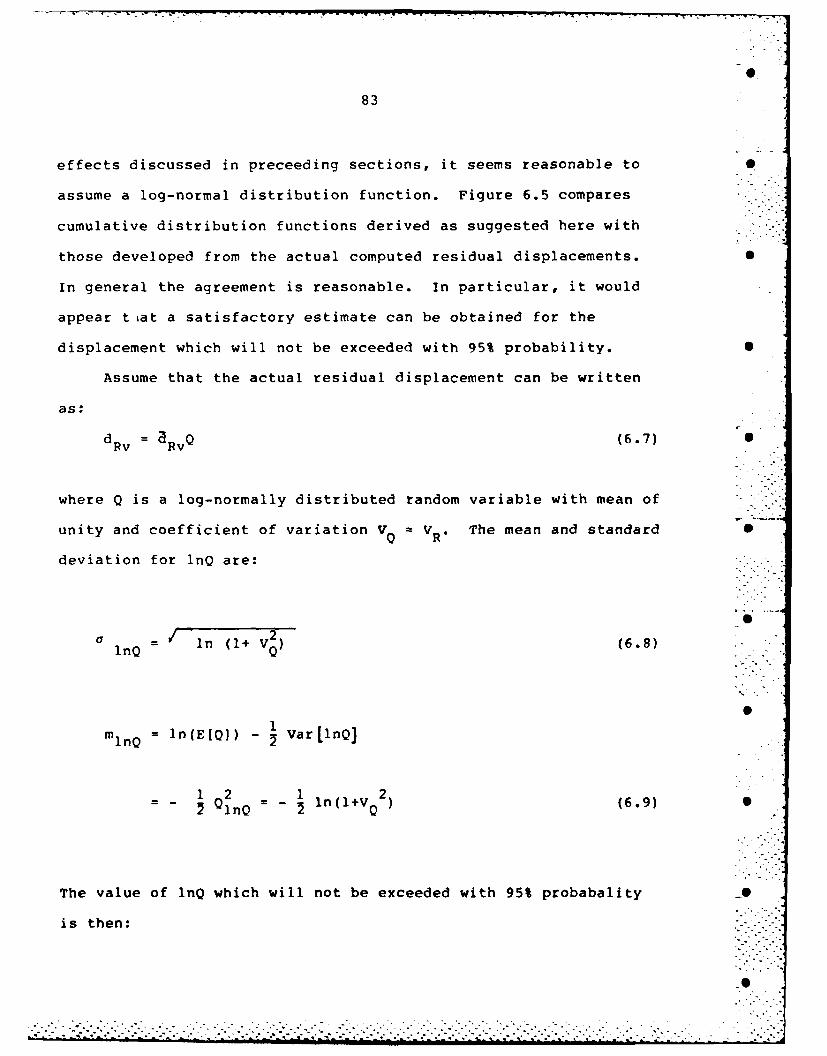
83

effects discussed in preceeding sections, it seems reasonable to S

assume a log-normal distribution function. Figure 6.5 compares

cumulative distribution functions derived as suggested here with - .

those developed from the actual computed residual displacements. S

In general the agreement is reasonable. In particular, it would

appear tiat a satisfactory estimate can be obtained for the

displacement which will not be exceeded with 95% probability. S

Assume that the actual residual displacement can be written

as:

d = Rv0 (6.7) S

where Q is a log-normally distributed random variable with mean of

unity and coefficient of variation V VR. The mean and standard S

deviation for InQ are:

2Sn = / ln (1+ VQ) (6.8)

mlnQ= ln(E[Q]) - • Var [lno]

-1 2 = 1 2Q ln(l+v (6.9)

-. -0lnQ ..,n-

The value of lnQ which will not be exceeded with 95% probabality _0

is then:

..............

. . . .. . . . . ..... ..•m.h ilm• •.. ..... . • . . . , - •. , , . ,

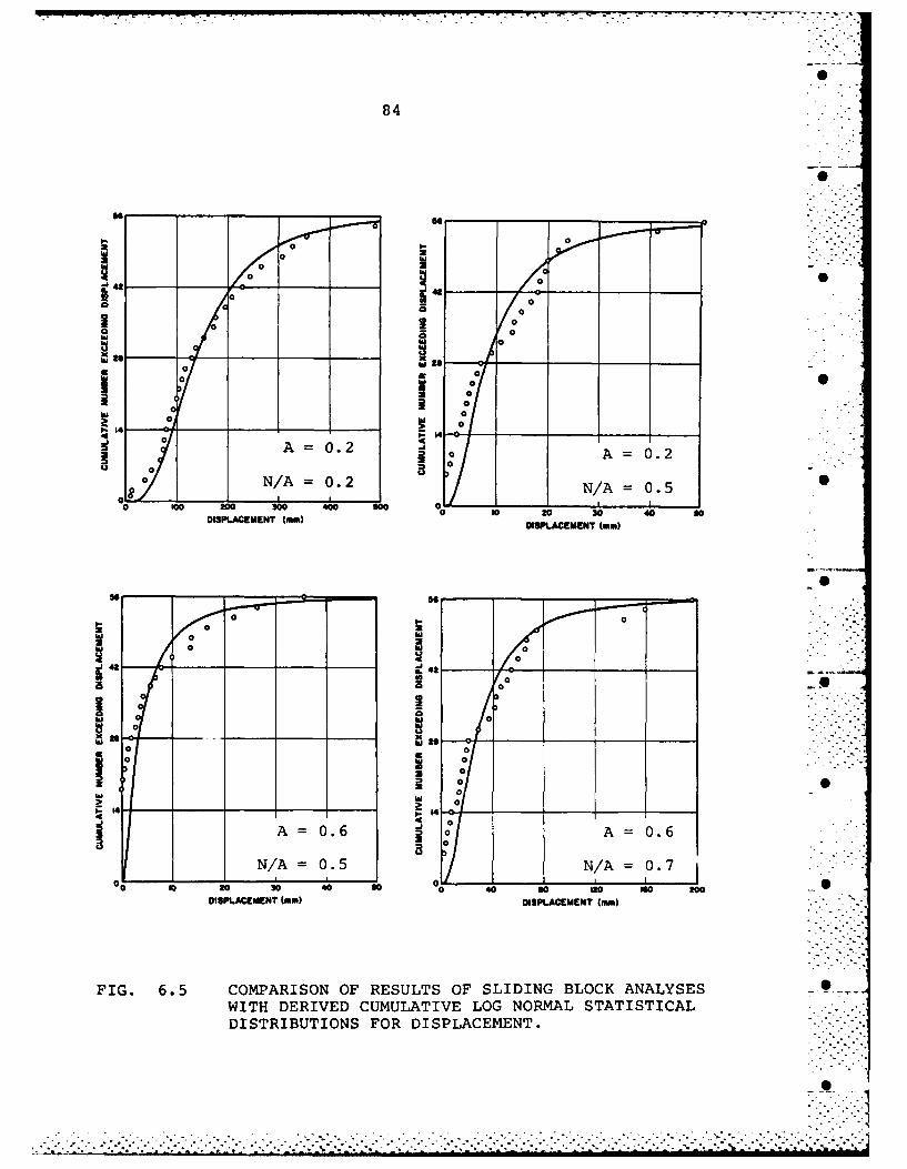
7 77

84

0 a

hI 0 0

8 00

0A =0.2A 0.0

0N/A= 0.2 N/A= 0. 5C

8 ~~ 1_ _

0 100 200 300 400 Goo Cv

OISPLCEMET ~DISPLACEMENT (me)

LOSS

00

0

N/ = 0.5NA 000 10 2 0 4 o0 4 o I9oI 0DISPACEENTtom)DISLACMEN

FIG.~~~~~~~~~ 0. OPRSNO EUT FSIIGBOKAAYEWITH DERIVED CUMULAT~~IVELGNRA TTSIA

DISRIUTINSFORDIPLAEMNT

85

0lnQ9 5 = mlnQ + 1.649 in1 (6.10)

or

lnQ9 5 I n (+V + 1.645 Vln (1+ VQ ) (6.11) .52 .

or

1n (1+ V) + 1.645 in(l + 2 (6.12)

- in-(1+ +.Vo95 e

Values of 095 are given in Table 6.4, for typical values of V0 .

The interpretation of these results is as follows. Suppose that

the allowable residual displacement is dL. Then, in order for .

there to be 95% probability that dL will not be exceeded during an

earthquake with given peak acceleration and peak velocity, then

the expected (average) residual displacement for such an earth- I

quake should be dL/Q 9 5 . This assumes that other parameters of a

problem, such as the resistance of a block or wall to the "

initiation of sliding, are known with certainty. The effects of •

uncertainty in these parameters as discussed in the next chapter. . .

6.8 APPLICATION TO RFTAINING WALLS S

As discussed in Chapter 5, for a given A, V and N the -

residual displacement of a retaining wall, d., is not equal to the

residual displacement of a sliding block. Thus Equation 6.2 does •

not apply exactly for the mean residual slip of retaining walls.

However, calculations by Wong (1982) have shown that the

86

Acoefficients of variation for dRe are very nearly equal to those

for dRe' for each A and N. Hence Equation 6.11 and the results in

Table 6.4 apply to retaining walls as well as sliding blocks.

6.9 IMPROVEMENTS TO PREDICTIONS

The procedure outlined here for predicting the average dis-

placement of a sliding block is, of course, only as good as the

suite of earthquakes used to develop the correlations and as the

assumption that A and V are the best measures of intensity of

shaking. It will certainly be desirable to refine and improve .

upon Equation 6.2 by using a larger suite of earthquake motions.

Another improvement will be to use several such suites, each for a

limited range of magnitudes (and perhaps epicentral distances) so

as to reflect the influence of the duration of motion. It may

also be that there are parameters other than A and V which are

better indicators of the amount of residual displacement than can

occur; for example, magnittle and epicentral distance. Explana-

tory studies into these questions are ongoing at MIT under the

direction of Prof. Daniele Veneziano. Finally, as noted in

Section 6.3, a more thorough treatment of the orientation effect

would be desirable.

- -

S . ,.

S

................................................... .. ..

87

7- UNCERTAINTY IN RESISTANCE PARAMETERS 0

1 INTRODUCTION

The analysis in Chapter 6 has assumed that the mean displace- 0

nt dRe is a known function of the properties of the wall and

ckfill. Actually, dRe is itself uncertain - partly because of

certainty in these properties and partly because of uncertainty 0

the model being used to compute displacement for given

operties and given ground motion input. This chapter deals with

e effect of uncertainties in the wall/backfill properties. 0

These properties include the weight of the wall; the unit

ight of the wall; the friction angles at the base of the wall,

thin the backfill and at the wall-backfill interface; and the S

ometry of the problem. While all of these properties are

certain to some degree, the most important uncertainties are

ose associated with the friction angles. The influence of

certainties in the other properties generally is insignificant,

ýd will be ignored in this analysis. That is to say, these other

operties will be considered as deterministic. S

Computation of the uncertainty in permanent displacement

ivolves: (a) evaluation of uncertainty in the friction angles,

id then (b) propagation of these uncertainties through the S

ialysis connecting the friction angles to permanent displacement.

ie latter step is described in sections 7.3 and 7.4, beginning -"-. -.

th the case of a sliding block on a horizontal plane. 0

..............

88

7.2 UNCERTAINTY IN FRICTION ANGLES

The friction angles selected for analysis of a particular

retaining wall seldom are based upon values measured using the

actual soils at that wall, but rather are estimated based upon

past experience with similar soils. Moreover, the actual friction

angles may change as sliding progresses. The uncertainty in

movement associated with this latter consideration should most

properly be treated as part of the model error discussed in

Chapter 8, but for purposes of this report it is considered as

resulting from uncertainty in the evaluation of the friction 6

angles.

When friction angles of a granular soil are measured,

starting from a specified initial density, scatter is relatively 0

small. It might reasonably be characterized by a standard

deviation a of 1 or 2 degrees. However, because the backfill

sometimes is poorly compacted and its actual density unknown, the

possible variation about the actual mean value must be greater.

Because backfill does tend to be loose, there is relatively little

decrease in friction angle past the peak value as strzining 0

continues. Furthermore, * for backfill is almost always selected

conservatively, and it is rather unlikely that the minimum value

can be more than several degrees less than the anqle typically S

used for design. (It is the possibility that the actual t may be

less than the value assumed for design that is of primary concern ..-

to us). All in all, it seems reasonable to use a. 2 degrees or

possibly 3 degrees.

-j -•-• -i >.• . .' - -i•''> > ' > >> :..' .' i- ... "• >>~i -> ii .: : " ". "." i3. -" i : . .. " . .-- '•-'>S .

I- .,...•..

89

These same arguments also apply to the friction angle *b at Sbithe base of the wall. Because foundation soils tend to be better

compacted, *b usually is greater than t. By the same token,

decrease in *b with continued sliding is likely to be more 0

significant. However, once again the values nominally used for

calculations are likely less than the actual mean. Again it seems

reasonable to use a standard deviation of 2 or 3 degrees. •

Engineers tend to feel quite uncertain as to the choice of a

suitable value of wall friction angle 6. It is not that the

actual peak interface friction angle is in great doubt, but rather .

there is uncertainty as to how much frictional resistance is

mobilized at a wall before static failure occurs. In the seismic

problem where slip is actually expected, this type of uncertainty .-

shvuld not be so important. Nonetheless, it is considered that a

larger standard deviation should be considered in the case of wall

0friction; say a6= 5.

For the calculations in the following sections, it is

necessary to pay careful attention to the units for the standard

deviations of friction angles, and this is best handled by S

re-expressing the foregoing results in radians. Appropriate

values are summarized in table 7.1.

7.3 BLOCK ON HORIZONTAL PLANE

When uncertainty in resistance is considered, the term d inRv

Equation 6.7 becomes a function of the random variable N; that is,

this term is itself a random variable. The variance of d may be

found by:

* ... -..... ... .. ..... .... *.. . . .. .. - .. .. -.

90

Table 7.

"ESTIMATED STANDARD DEVIATIONS"FOR FRICTION ANGLES

Location a in radians

Backfill 0.035 to 0.052 .0

Base 0.035 to 0.052

Wall 0.035 to 0.087.o .S

. , -.

* ... •

91

S

2• [2

Rvv 8N1

i~ 2

Var~dRy I = [--gf- Var[N] (7.1)

Alternatively, but less precisely, we may rewrite Equation 6.6 as:

dr dRyQR, (7.2)

where now R is a deterministic function computed using average

values for the friction angles involved in the problem at hand and ".

R is a random variable with mean unity reflecting uncertainty in

the friction angles. The variance of R is given by Equation 7.1.

Computations show that 83Rv/bN is closely approximated by . •

1/N. Hence the variance of R* may be expressed as:

2_ a 37V2 -9 4/A) 2

Var[R e9 (-- ] Var[N] (7.3)Va [@]= Fv 8N A

[_14 2= (_-j Rv 2] Var[N]

Taking the square root to obtain the standard deviation of R and

dividing by 0Rv' the coefficient of variation of R becomes:- .

Vrj, 9.. (7.4)

.-.. .. . -.-........ . -. . . . . . . . . . . . . . . . . . . . . . . . . . . . . . .. . . . . . . .- .-. -. .~

--

92

Note that V R is inversely related to the ground acceleration S

coefficient A. This means that, since it is ratio N/A that

determines the amount of slip, a given uncertainty in N is much

more important when A is small than when A is large.

For a sliding block of known weight on a horizontal plane,

the transmittable acceleration N is determined entirely by the

friction angle between the block and the supporting plane:

N = tano (7.5)

The variance of N is then found by:

DN2 4Var[N] = [.] Var[4] = sec4q Var] (7.6)

and the standard deviation aN is:

aN =a c/cos 2 • (7.7).

Typical values for * range from 300 to 350. Using the values for

a, from Table 7.1, the range for aN is 0.05 to 0.08.

Combining Eqs. 7.4 and 7.7 leads to the results in Table 7.2. -Note that some of the values of V - those for the smaller A -

are quite large, much larger than the coefficients of variation .. -

discussed in Chapter 6. Thus it is evident that uncertainty in -

resistance parameters can be a very important consideration.

. . .. .

93

Table 7.2

COEFFICIENT OF VARIATION OFRESISTANCE TERM

VR

A aN -0.05 aN 0.08

0.2 2.35 3.76

0.3 1.57 2.51

0.4 1.18 1.88 O

0.5 0.94 1.50

0.6 0.78 1.25

0.7 0.67 1.07 S

S,•

: S:.,: .

.S

"S":

_O

94

7.4 RETAINING WALLS

For retaining walls one proceeds in a generally similar

fashion. In this case, an exact solution would require

derivatives for the product d • R Values of the partialR 2/1'Vle f h ata

derivative have not been evaluated, although approximate results

by Wong (1982) indicate that the value obtained for a sliding

block are a good approximation for the retaining wall case. That

is to say, Equation (7.3) may still be used. Hence interest then

focuses upon evaluation of Var[N] for retaining walls. .

The variance of N depends upon uncertainty in the three

angles 0, *b and 6. If these angles are assumed independent of

each other, then Var[N] may be evaluated by:

ýN 2 2 + ý)2Var[N] = + Var[ýb] + (-) Var[61 (7.8)b D6

The derivatives are obtained from Equation 4.4, which may be

rewritten as:

[cos (p+6) -sin (p+6) tanOb] PAEN =tan~b - W (7.9) .- "

w

Since PAE is a function of N as well as of * and 6, implicit

differentiation must be used. Wong (1982) carried out the

necessary steps, and the resulting equations are reproduced in -

Table 7.3.

Numerical evaluations of these equations have been performed .

for various combinations of values of the three angles and of N.

• . , i- i- ? >~ - .. l•i-lllll2 .l- lli'.- ~ ~ - ii....- . -.. , • . -.- ... • -i -i. .ili-i. i •i..i . .: i'• i .-.

95

Table 7. 3

EQUATIONS FOR PARTIAL DERIVATIONS OFN WITH RESPECT TO ý, b AND ~

-N Ge [ b F cot(a+6 ) -N

3ý b G L~ot (+6) -tan~b) (tan~b -N)J

IN 1. [2r nOýa cot (0+6) +cot (o-i-i)1-~~~~~~ G jtn(--)+1+ j

ýN _1 [cot(ct06)-Jtan(iP+ý+6) tan(a-I6 )+tan b1+CY L 1 + J l-tan(ý+6 )tan ýbj

G Ptan+N2 -ý + N + cot (ý-ý-i) +Htan ('P+a+

+tan -N

/cos (i-a)cos (t+a+6)sin ý6sin(ýýi

96

(All have involved • = i = 0.) One special case of some interest

is that when *b = * and 6 = 0. Then equation 7.8 may be rewritten ---.

as:

Var[N] [ +(N) + IN Var[p] (7.10)

The term in brackets is nearly constant for the several combina-

tions investigated, at a value of about 0.85 radians-2 Thus:

aN= /8 = 0.92a (7.11)

That is to say, the uncertainty in N is actually somewhat less

than that in each of the two friction angles. This reduction

occurs because, assuming independence, it is relatively unlikely

that both friction angles will be simultaneously larger (or

smaller) than mean values. If there is some actual dependence

between the values taken on by these angles, then the ratio aN l

would be increased to some degree.

When wall friction is present, as indeed it must be, the

situation is more complicated. Results from some typical calcula-

0tions are presented in Table 7.4, for the case = a =b 2 = a

05 and 0 = i = 0. It may be seen that a varies with the

combination of values used for the three angles and N, and is

greatest when N is smallest. Somewhat greater values of aN may be

found when other combinations of parameters are used. Further-

more, depending among the three friction angles (especially

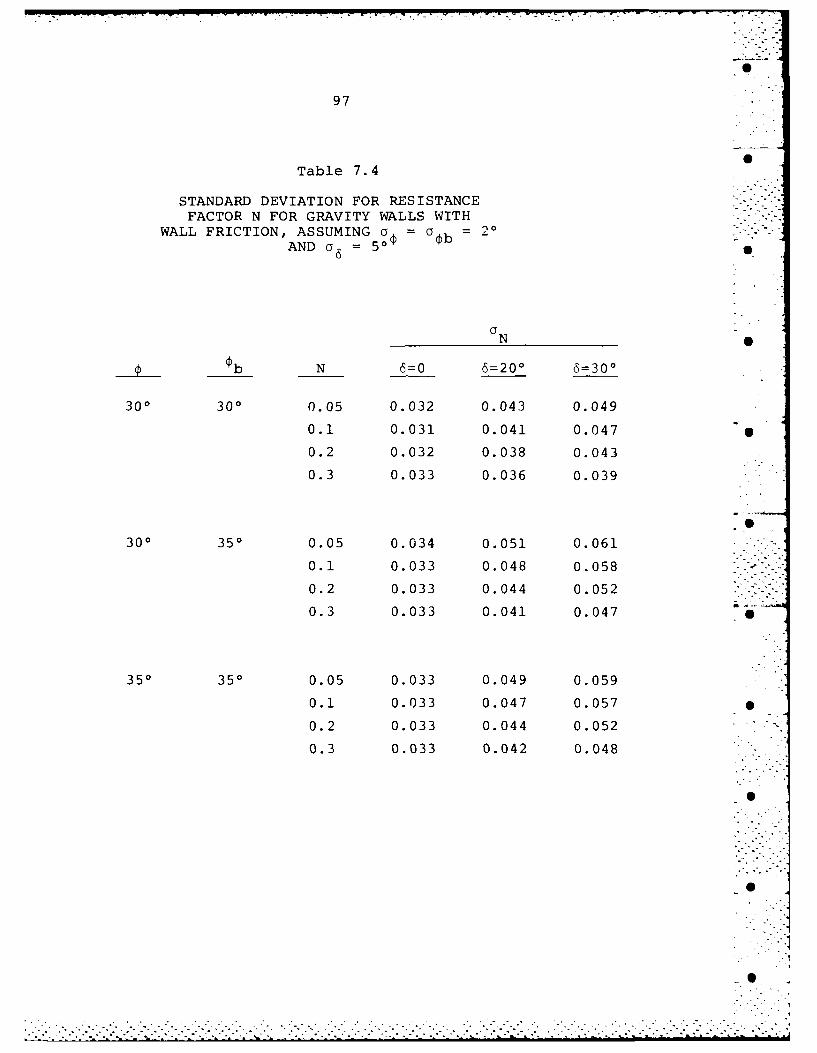
97

Table 7.4

STANDARD DEVIATION FOR RESISTANCEFACTOR N FOR GRAVITY WALLS WITH

WALL FRICTION, ASSUMING a = b =AND 06 = 504 pb

N

_b_ N 6=0 6=200 6=300

300 30 0 0.05 0.032 0.043 0.049

0.1 0.031 0.041 0.047

0.2 0.032 0.038 0.043

0.3 0.033 0.036 0.039

300 350 0.05 0.034 0.051 0.061

0.1 0.033 0.048 0.058

0.2 0.033 0.044 0.052

0.3 0.033 0.041 0.047

350 350 0.05 0.033 0.049 0.059

0.1 0.033 0.047 0.057

0.2 0.033 0.044 0.052

0.3 0.033 0.042 0.048

S

0

S- . . -

98

between o and 6) will cause the aN to increase. It was judged

that an average of the numbers in the final column of Table 7.4 "

would be most representative of the uncertainty in N, and such

average values are plotted in Fig. 7.1 as a function of N.

Values of aN may be entered into Equation 7.4, and Table 7.2

is still at least approximately valid. Once again the conclusion

is that the overall effect of uncertainty in the friction angles

is very significant.

S .. .•

S :i i

S

-S

S

S"m" "" • " ; • "i " • • "•" " m "Ia• • "( • " " "

99

0.08

0.06

0-N 0.04 -(

0.02

S

00.I 0.2 0.3

N

FIG. 7.1 TYPICAL VALUES FOR N FOR RETAINING WALL WITHWALL FRICTION. N

. . . . . .. . . . . . . .

100

8- MODEL ERRORS AND UNCERTAINTIES

This chapter discusses several ways in which the two block -

model of Chapter 5 is still imperfect, but where knowledge is

inadequate to permit use of an improved model. These aspects

include the proper choice of a failure plane, the effect of

deformations within the backfill before sliding begins, and

tilting of walls. In addition, there are errors because one may

choose to use simpler approximate results in lieu of expending

considerable effort in using the best methods of analysis that are

available.

8.1 FAILURE PLANE INCLINATION

In Zarrabi's (1979) two-block model, it was assumed that the

inclination of the failure plane in the backfill varies with the

instantaneous ground acceleration. This is a natural assumption

that arises from the formulation and application of the Mononobe-

Okabe Equation. However, as described in Chapter 2, the model

tests performed by Murphy (1960) and Lai (1979) indicate that it S

may be more reasonable to assume that the failure plane inclina-

tion remains constant during slip. Jacobsen's (1980) comparisons

of Lai's (1979) model test results with calculations using the

two-block model concur with this reasoning, in that the agreement

is better between theory and experiment, when a fixed angle of

inclination o is assumed. Thus, it would be reasonable to use a

fixed angle 0 in the calculation of residual displacements.

114

depth more rapidly than linearly. At other times when the 5

rotational acceleration of the wall reverses, the opposite is true -

and then the resultant horizontal force lies above the lower third

point. 0

Once revealed by this simple conceptual model, these results

are quite obvious. The analysis demonstrates clearly that

conventional wisdom concerning the location of the resultant,

which was derived for the case of a wall that does not tilt, may

be quite misleading as regards the response of a wall which is

free to tilt. 0

Nadim used this model to study the relative importance of

sliding and tilting. Moment resistance at the base of the wall

was assumed to be rigid-plastic in character, and it was further 5

asumed that the axis of tilting was at a fixed location. A

threshold transmittable acceleration, NR' is reached when the base .

moment required for dynamic equilibrium just equals the maximum •

moment. (The dynamic stress from the backfill is assumed to

increase linearly with depth in this calculation.) Any tendency

for the thrust from the backfill to increase further is resisted 0

by rotational inertia of the wall. The principal conclusions from

Nadim's study were:

Tf N > N, then only sliding will occur. That is, havingR

resistance to sliding which is less than the resistance to

tilting protects the wall against tilting.

If NR < 0.85N, then only tilting - and no sliding -

occurs. In this case, the permanent displacement at the

•-

113

0

,all may slide and/or rotate about its base. The horizontal

icceleration of each slice is just equal to the horizontal

icceleration of the wall at the point where the slice meets the

pall. Each slice also accelerates vertically, as necessary to

iaintain contact between the slices. With these various

issumptions, it is possible to develop an equation giving the

listribution of stresses between the wall and backfill in terms of

he horizontal acceleration of the wall at its base (which may

liffer from the acceleration of the underlying ground) and the

otational acceleration of the wall. This equation is then used

.ogether with equations for the dynamic equilibrium of the wall

as in Chapter 5) to compute the motions of the wall.

One result of this analysis - a rather surprising result at

irst sight - is that the resultant of the dynamic stresses

)etween backfill and wall sometimes lies below the lower thirdS

point. This happens whenever the tilt of the wall away from the

)ackfill is accelerating while the horizontal acceleration of the

[round is towards the backfill (which is just the situation of0

freatest concern to us). At such times (see figure 8.5b), the

ibsolute acceleration at the top of the wall is less than the

ibsolute acceleration at the base of the wall. With our

issumptions, this means that the uppermost slice through the

)ackfill has a smaller acceleration than the slices below it.

lence the horizontal stresses between soil and wall increases with

It turns out that the thickness of the individual slices can inthe limit be set to zero, so that a continuous equation isobtained.

112

ol IIA

4e. U3

Ns S- 0l

In 00

0 E- 0

~~0 u

0H S

O E-4O

C-0E-4Z

tipii-

"P4 = .

NN N

HD

* . . .-

111

depicted by the dashed "proposed design lines" shown in Fig. 8.4.6

The factor RE obtained from these lines can be justifiably used as

relatively conservative amplification factors to be applied to

simpler sliding block analysis, in the same vein as previously S

suggested.

It should be noted that the fundamental frequency fBF for

backfills will typically range from 5 Hz to 25 Hz. Dominant S

frequencies of ground motions fE-Q range generally from 2 Hz to 5

Hz. Thus, the most typical range of the frequency ratio fE-Q/fBF

is 0.2 to 0.6.

8.3 TILTING

Observations in the field following earthquakes suggests that

permanent displacement of gravity retaining walls usually involves

tilting. This important aspect of behavior has received very

little attention from a theoretical standpoint, and hence is still

poorly understood. There have been model tests in which a wall is

tilted while it and the backfill are subjected to earthquake like

motions (Sherif, et al. 1981). These tests have confirmed the

influence of tilting upon the development of active conditions

behind a wall. However, they give no direct evidence as to the

amount of tilting that might develop in a free-standing wall.

A preliminary study of this problem by Nadim (1980) used the

conceptual model shown in Figure 8.5. The failing wedge of soil

is subdivided into thin slices which may slide over each other S

once frictional resistance on the interslice failure surface is

reached. Except for such sliding, the backfill is rigid, while the

S. .

110

idealization of the problem. In all of these cases, it was

assumed that there is a rigid boundary beneath the backfill at the

same level as the base of the wall. This means that seismic wave

motions reflect back into the backfill from this boundary.

However, in most real problems this boundary is not rigid, and a

portion of the waves radiate away from the region of excitation at

this boundary (radiation damping). Because of this effect, the

actual amplification of ground motion through the backfill is

probably not as large as one predicts from the finite element

analysis with a rigid boundary at the level of the base of the

wall, especially near resonance conditions.

Another trend shown in Fig. 8.4 is that the amplification of

residual displacements is more significant for high values of N/A.

If N/A = 1 and the rigid block model were correct, there would be

no slip. However, because of amplification through the backfill

the acceleration in the upper portions of the backfill would

actually exceed N, and hence slip would occur. Thus for N/A equal

to and slightly greater than unity, the ratio R is infinite. AsF

previously noted, however, the usual range of practical values of

N/A is from about 0.3 to 0.7.

The incorporation of preceeding observations into a practical

design criteria can be done in several ways. Nadim (19P2) and

Nadim and Whitman (1983) have proposed modifying the values of A

and V to reflect the amplification of ground motion, and using

these amplified values of A and V as input into a block model

analysis, such as the Richards-Elms Equation (Eqn. 4.1). An

alternative method that is perhaps simpler and more direct is

0109

0

d using elastic finite elementsR

RE = d using rigid 2-block modelE R

The variables f and T are respectively the dominant .

frequencies and period of the earthquake excitation, and f andBF

T refer to the first fundamental frequency and period of theBF

backfill.

From Fig. 8.4, it is clear that much larger displacements

than predicted by the rigid-block model can occur if the

elasticity of the backfill is considered, as in the finite element S

model. The ratio R can become very large (on the order of 10) as

the ratio of the frequencies fQ/fBF approaches 1.0, which is

analogous to a resonance condition for a SDOF vibrating system. S

Since the fundamental frequency of the backfill can be

approximated as

BF C s (8.4)4H

where Cs is the shear wave velocity of the soil and H is the

height of the wall. This implies a direct correlation between the

frequency ratio and the height of the wall. Thus the amplifica-

tion problem is more pronounced for higher walls.

It should be noted the finite element results obtained for

excitation frequencies near the resonance condition are conserva-

tive because of the boundary conditions that are imposed in the

................................... ..........-.-- ,•_-

S

108

E-0 -

N 0 E

-E-

ODo

0 0E-

E..-m...:zz

0S

0 0

E-4c0 I. OH"

SZz z .

444

0 Uo 0-4 ri•~ 00

o "IC.-,. - ,---,•- € i_ O

c 0 HOr.~ EE E-6

W ~0 Cl)'

i 00 sl) 0 LO 0

13001N a07oie -z a]li8 buisn Up

SIN3fl313 3IJNI OI1LSV713 buusn Up =L"

...................................-..........-.... .... -. '.--:. ........ . ."... .'.......'. .. ". ... '

107

increases the ground accceleration coefficient A. Assuming that 0

the transmittable acceleration Ng is approximately the same

regardless of the flexibility assumption, the effective N/A ratio

would be lower for the flexible backfill than for the rigid back- S

fill case. Consequently, considering the results from rigid block

models, larger residual displacements would be expected. Also,

there is additional amplification of the transmittable accelera- S

tion coefficient, such that larger earth pressures would be

expected to develop, if envisioned in the context of seismic

coefficients. S

Obviously, the preceeding statements are only intuitive

arguments for explaining how ground motion amplification affects

residual displacements. It should be recognized that the concepts ',

of rigid block models, including strict quantifications of N, A,

v2/the ratio N/A, and notions of normalizing displacement using V2/Ag

are no longer valid in view of the non-uniform distribution of 0

these quantities in an elastic finite element model. However, the

corresponding rigid block model quantities can be calculated and

can serve as useful references for comparison of results. S

Numerical results from the elastic finite element model

results as compared with those from the rigid two-block model

(assuming constant e) are in Fig. 8.4. Computations are shown for 0

three earthquake records and two different values of N/A. The

format of comparison is analogous to the frequency response cure

for a single degree-of-freedom (SDOF) vibrating mass. The ratio .0

RE, a residual displacement amplification factor, is defined as:

ES~. . . .. . . . . . . . . . .

- "- - .--- -. :-- .-.- .. - . . . .. . . - ....-.. . "•, =.• _ : . . . -.. -"- -" . . . -" - ." - .- , -" -.- , -'- - -•, -".,.- .. .-

106

Some ambient ground motionat both locations

Acceleration constant"' ~within block

(a) Rigid Blocks and Backfill S

Ground motion amplifiedby elastic backfill

2'/ -

Ambient ground Acceleration variablemotion and amplified in block

(b) Flexible (Elastic) Blocks and Backfill

FIG. 8.3 SCHEMATIC COMPARISON OF EFFECTS OF RIGIDITYAND FLEXIBILITY (ELASTIC) ASSUMPTIONS INRETAINING WALL BEHAVIOR. 5

--7, .

.)iii:

105

:1 0

because of lack of data. However, in terms of practical signifi-

cance, for the ranges of N and A commonly encountered, whether one

uses a fixed or variable 8 may not be important. This is

especially true in light of the uncertanties in evaluating 8 (as

shown in Fig. 8.1) and the even larger uncertainties in the

earthquake ground motion characteristics.

8.2 ELASTIC BACKFILL EFFECTS

The sliding block model developed by Zarrabi (1978) assume

the blocks representing the retaining wall and the soil backfill

wedge to be perfectly rigid. This is actually a fairly good

assumption, particularly for walls with relatively low heights, -

where the effects of wall and backfill flexibility are essentially

negligible. However, for high walls, the rigidity assumptions may

lead to severe underestimation of the residual slip. The effects".

of assuming the wall and backfill to be elastic, and hence

flexible, has been studied by Nadim (1982) using the finite

element idealizations as described in Chapter 2. These result

have also been reported in a paper by Nadim and Whitman (1983).

The basic effect on an elastic backfill is the resulting

amplification of ground motion, similar to the phenomenon which is

expected to occur in earth dams (see Seed and Martin, 1966 and

Makdisi and Seed, 1979). The amplification phenomenon is schema- .

tically illustrated in Fig. 8.3 and compared to the rigid block

case, without amplification.

Firstly, amplification of the ground motion occurs in the

backfill outside of the soil failure wedge, and effectively

104

0

z w~

O 0

U)

o 0

IzUS dw --

z - 0

"c H

tun OW x 4

0 OD

04X

IOXl bu)Z U

... .. . .. .. . ... .

0I4

8 0 X-I 0us p " -.. •N.::..: :rz.:.

0 i --

. ° . . . _ - . . -. - . . - . - . . j 2 "j - - . o. . , - / . . -, . . o . • . . . .. - . " . " . , • . . • -O " .' '.. . .- ,. . ... .•., .-..•-..... ... • . .. . ... .. • . . . .. . • : .- . . ., ,. , , .. ; ,.,.. .. , ,.- --. , . . ,, ,.-. .,, .C,., -U).-.-

103

(increasing F ww), a larger inertia force from the backfill is

required to initiate slip. Thus a larger mass of backfill soil

"" must be mobilized as reflected by a decrease in ..

The experimental results for 6 shown in Fig. 8.1 are consis-

tently higher than the theoretical threshold eTV calculated based

on measurements of 0, *b and 6 evaluated by Lai (1979) and

Jacobsen (1980). This may be attributed to frictional effects

between the model and the glass sides of the model container,

which would tend to effectively increase *. There is also a range

of possible interpretation of the failure angle 6 due to the fact

that the failure surface is actually a zone rather than a thin

line of failure. Furthermore, there is a slight curvature to this

failure zone, deviating from ideal linear conditions. 0

The numerical differences that arise in the calculated

residual displacement between assuming a constant or variable

plane of failure are illustrated in Fig. 8.2. The results shown

are obtained from calculations performed separately by Nadim

(1982) and Wong (1982) using three earthquake records and a

constant value of N = 0.112. The Ratio Re is defined as:

R Residual displacement using fixed 0 (8.2)8 Residual displacement using variable e S

The value of R8 is generally less than or equal to one, with

those values greater than one thought to be the result of

numerical round-off errors. There is clearly a trend toward

greater discrepancies for increasing accelerations, given a fixed

value of N, but further generalizations of trends are difficult '

"................ • *- i " t*' .'." .... ... . .'• "....-... . .. " -°"... ... """'

102

0

0

"E-z

z

Cd 0

0 z.

- N 0E- -

~0 3

0 w 0

0 pO

4 "0 co1-

0~ a-

0CJ ..- I--4 00

00

44

101

J Physically, once a failure plane develops in the backfill,

the plane may become slightly weaker than the surrounding soil and

it would be the preferred plane of failure at subsequent stages of

movement. Thus, the initial failure plane that develops should

logically be used in the analysis. Thus the critical failure

plane angle of inclination 0T which would occur during earth-

quake motions is only dependent on the wall weight and the

properties of the foundation and backfill soils. Nadim (1982)

gave equations that determine the angle of inclination of this

plane explicitly as:

OT = 1/2(a + a,) (8.1)

where a = tan-1 (B/A)

a1 = cos -1 (-C.cosa/A)

and

A = cos(4+6+i)sin(4b-) - sin(+6-i)cos(b-

- cos(i)cos( 6 +$b)F

"B = 2 cos(i)sin(s b- )sin($+6)

C = sin(o b+6+i) - cos(i)cos(6+sb)/Fww

W"

F = w 2 wall weight factorww i/2yH2

A comparison of the theoretical equation give by Nadim (1982)

and the results from Lai's (1979) experiments is shown in Fig.

* 8.1. Both theory and experiment show a general downward trend for

8 with increasing wall weight factor Fw. This downward trend isww

explained physically by the fact that as the wall becomes heavier

. . . . ...•. - • .. . ..-.-- ..--' • • , ' .,.- .d a '.:.= • . . . . . . . . . . . . . . ..- ,.' ," " : : % " " •" "

115

top of the wall was found to be about 1 1/2 times the

movement predicted using a sliding block with N set equal

to NR. Thus there's some reason to think that a sliding

block model maybe useful in estimating permanent

displacement even though tilting is the predominant mode

of displacement.

These conclusions must, of course, be treated with great caution.

Unlike the case of sliding, significant tilting may occur

before the maximum resistance against overturning moment is

reached. There has been no adequate study of this aspect of the

problem. Some results obtained using the finite element model of

Figure 2.5 have confirmed that the resultant thrust from the

backfill can lie below the lower third point at various times a

during a cycle of shaking. It does seem clear that any tendency

".- for a wall to tilt will relieve the overturning moment acting upon

the wall. ""

All in all, there is reason to believe that the sliding block

model proposed by Richards and Elms is a reasonable model for

predicting the permanent movement of actual gravity walls,

provided they have been designed using a typically conservative

' safety factor against overturning by static loads.

8.4 APPROXIMATIONS TO 2-BLOCK ANALYSIS

If one knows the inclination of the failure plane through the

backfill, or if one is willing to accept the assumption that this

inclination varies continuously during shaking, the effect of

kinematic constraints can be taken into account as discussed in

•. • ., .• • > '• •- .i .-- . .. • . . .- ' -. •- } -'-•} .•- -/ .. -• .. } .•. . . .• .. ..- ••* *.* .*. - '. '.- *: ' *.' .'*.*. " . . .. :.* .

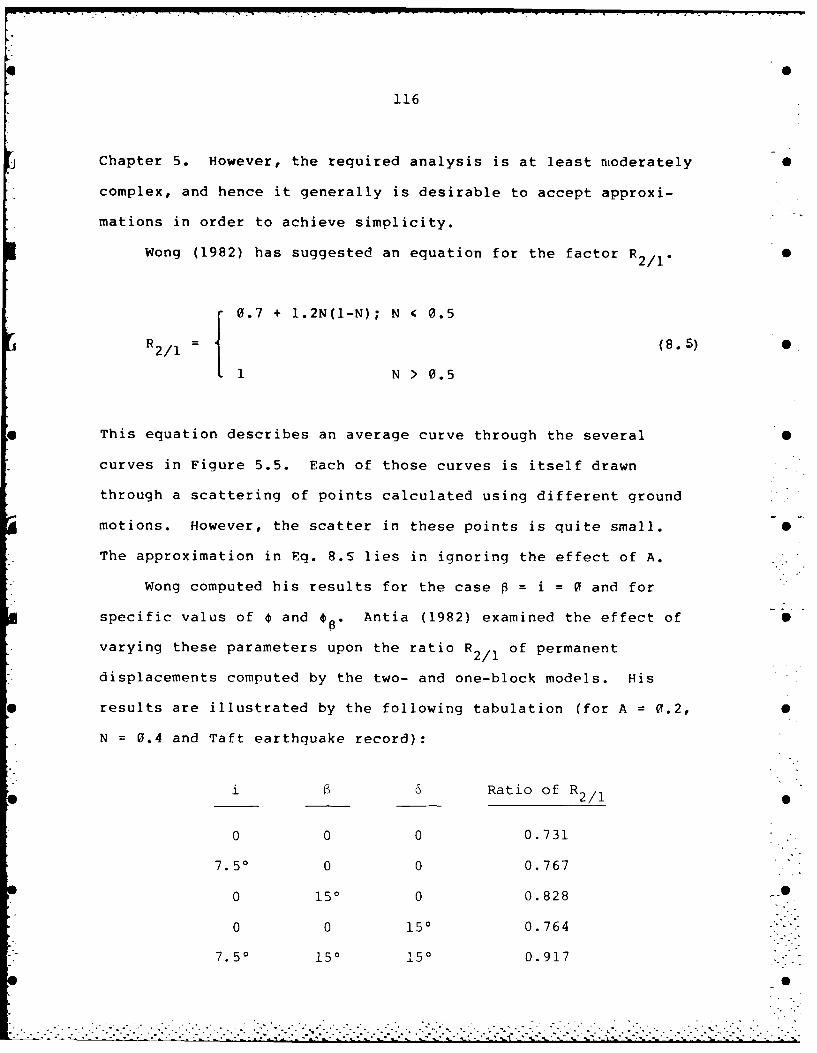
0

116

j Chapter 5. However, the required analysis is at least nmoderately S

complex, and hence it generally is desirable to accept approxi-

mations in order to achieve simplicity.

Wong (1982) has suggested an equation for the factor R2/ 1 . '

[0.7 + 1.2N(l-N); N < 0.5

R2/1 = (8.5) 0

1 N> 0.5

This equation describes an average curve through the several 0

curves in Figure 5.5. Each of those curves is itself drawn

through a scattering of points calculated using different ground

motions. However, the scatter in these points is quite small.

The approximation in Eq. 8.5 lies in ignoring the effect of A.

Wong computed his results for the case f = i = 0 and for

specific valus of 0 and *8" Antia (1982) examined the effect of S

varying these parameters upon the ratio R2/1 of permanent

displacements computed by the two- and one-block models. His

results are illustrated by the following tabulation (for A 0.2, 0

N = 0.4 and Taft earthquake record):

i 6 Ratio of R2 / 12/1

0 0 0 0.731

7.50 0 0 0.767

0 150 0 0.828

0 0 150 0.764

7.50 150 150 0.917

117

In all cases investigated, the effect is to decrease the S

difference between the residual displacements computed using the

two models. Wong reached similar conclusions. Note that each -

case in the tabulation above corresponds to a different weight of 0

wall, so as to hold N constant.

These results, plus those discussed in Section 8.1, emphasize

the complexity of the so-called "2-block" effect. There is no •

doubt that the effect is real and that it acts to reduce the

actual permanent sliding compared to that predicted using the

Richard-Elms simple sliding block model. The problem is in .

predicting this reduction accurately by any simple calculation.

Having the inclination of the failure plane fixed tends to make

the reduction greater than suggested by Eq. 8.5. As the results

in Figure 5.6 show, this reduction can be very large indeed. On

the other hand, Antia's results show that this equation may not ...-

always be conservative. -0

Taking all these factors into consideration, it is reasonable

to use a mean value of 0.65 for the factor R2 /I, and to represent

the uncertainty in this factor by a standard deviation of 0.2i S

.~~~- .. .-. .. .

IdS -

• '.

S ,

............................................................................

........................................................ ,...---._-.....

118

9- IMPROVED APPROACHES TO DESIGN

9.1 REVIEW OF OBJECTIVES

As discussed in Chapter 1, the general objective of this 0

study has been to quantify the uncertainties invovled in using a

displacement-limiting approach to the design of gravity

retaining walls for seismic loadings. The specific goal has 0

been to select, with greater confidence, a suitable safety

factor for use with the Richards-Elms approach or, if possible,

to develop an improved design methodology. In so doing, the S

desire to maintain the essential simplicity of the Richards-Elms

approach has been an overriding consideration.

The various aspects of the problem have now been examined, S

to the extent that knowledge permits. The next step is to

synthesize them into a unified approach to design.

S

9.2 EQUATION FOR PREDICTING MOTIONS

At the heart of any displacement-limiting approach to

design is an equation for predicting displacements in terms of S

the specified ground motions and the physical parameters

characterizing a gravity retaining wall and its backfill. To

achieve the objectives of this study, such an equation must be S

probabilistic in nature. That is to say it is necesary to

quantify the probability that various amounts of permanent dis-

placement will be exceeded. _

Equation 1.1 was suggested at the outset of this study for >--

this purpose. In it, the permanent displacement of a retaining

. . . . . . . . . . . . . . . . . . . . . . . . . . . . . .. .

119

wall is predicted by the product of five terms:

dR : The permanent displacement of a one-way slidingv

block with maximum transmittable acceleration Ng,

averaged over all earthquake ground motions

characterized by peak acceleration Ag and peak

velocity V.

R2/1 : A deterministic factor accounting for the effect of

a kinematic constraint ignored when using a sliding

block to represent a retaining wall and its back-S

fill.

0 : A random variable with mean of unity, describing the

variation of permanent displacement aroused by

different earthquake motions all having the same Ag

and V.

RO :A random variable with mean of unity, describing the

effect of random uncertainties in the resistance

parameters for the wall and backfill.

M A model error term, random in nature, which accounts

for as yet poorly understood aspects of the

p problem.

The first four of these factors have been studied in

considerable detail: R2 / 1 in Chapter 5, dR and Q in Chapter 6

and RO in Chapter 7. Methods for accounting for these several

aspects of the problem have been developed in some detail.

However, several of these methods are rather complicated.p,

•. ..:. .. *. .-....-. -. .... . . -... . . .-. -.. . .- . ... .- .. .--. .- .- .. . . . ............-.... -.. ..-....- ... *. .. .. . •.- . . . . . . . ."--- '- '" - ''" ' " -" "- : -:" -""- ... "" - :,,, * ,, ',, ; .. . "". . . ". ".".". "". . '.". . " "° " '. .' " " : ": --' " "-• '• ' "' :: :

120

The effect of vertical ground accelerations enters into the

expression for dR, and this causes the factors A and N to enter

into computations in a complex fashion. Complicated calcula-

tions are necessary to arrive at exact values for the ratio

R2 /1 , and this ratio is influenced by A and N in a non-simple

way. Similarly, it is not an easy matter to evaluate the effect

of deformable backfill, even though guidelines for this purpose

have been suggested in Chapter 7.

In order to retain simplicity, and keeping in mind the

still imperfect state of our knowledge, Equation 1.1 has been

simplified to:

d 37V2 -9.4N/A (9.1)(9.1dRw -ge " Q RM (9.1).

..

Ag

The first term is Equation 6.2 for the mean displacement of a

sliding block with no vertical ground accelerations. The errors

caused by ignoring vertical accelerations, and those introduced

by omitting the factor R2/1, are lumped into the model error

term M. N is the expected (in the average sense) threshold

transmittable acceleration coefficient for the wall/backfill,

evaluated using average values for the various friction angles.

Q, R2/1 and M are all random variables, Q and R having means of

unity. Based in part upon available numerical results (see

Chapter 6) and in part upon the form of Equation 9.1 (i.e. it is

a product of random variables) it is assumed that dR is

lognormally distributed.

0 i

* . rr r ~ r . - V -. -

121

Using results from the theory of probability and assuming

that Q, Rý and M are also independent, it is now possible to

write expressions for the mean and stantard deviation of dRw:

Mend 37V e-9.4N/A (9.2)Mean [dRw] = Ag e

where M is the mean value of M7 and *

2 94• 2 Na 2 (9) a 2 + a 2 + a 2nndRW A N .M lnQ

Actually, Equation 9.3 gives the standard deviation for lndR•,

rather than for dRw directly. alnM and alnQ are the standard

deviations for InM and lnQ, respectively.

Information concerning the parameters in Equations 9.2 and

9.3 has been summarized in Table 9.1. Coefficients of variation

for Q are found in Table 6.37 since the mean of Q is unity, the .

standard deviation equals the coefficient of variation. OlnQ is

computed by: S

G = ln(l+VQ2) .4inQ Q

Estimates for aN were discussed in Chapter 7.

The model error term M is a composite of several factors,

as indicated in Table 9.1. Figure 6.4 has been used to estimate

* In a more proper derivation, Equation 9.1 should have beenwritten as:

in dRw n( )) .4 + log Q + log m.

where N is a random variable. The first term in Equation 9.3is then obtained by employing:

n RN Var[N] = (- ) a 2

L 3N- A N

122

Table 9.1 S

SUMMARY OF PARAMETERS IN EQUATION 9.1FOR PREDICTION OF PERMANENT DISPLACEMENTS

Log normalStandard Standard

Factor Mean Deviation Deviation

Ground motion factor Q 1 0.6 -1.4 0.58-1.05

Resistance factor N N 0.04-0.065 -

MODEL ERROR

Vertical acceleration 1.2 0.2 0.2

Ignoring R 0.65 0.2 0.3

Deform, backfill 3 2 0.6 .

Tilting 1.5 0.75 0.5

Combined model error 3.5 3.6 0.84

S

w I ..I

.. . . . . .. . . . . . . ..".-

• , ,"

123

the mean and standard deviation of the error introduced by 0

failing to take the effect of vertical accelerations into

account directly. The discussion in Section 8.4 has provided

the basis for estimating the effect of not accounting directly 0

for the ratio R2 /1. Similarly, rather than introducing a

correction for the effect of deformable backfill as a function

of period ratio and N/A, a mean correction and a measure of 0

scatter have been estimated from Figure 8.4. The possible

effects of tilting have been discussel in Section 8.3. In

arriving at these various values, attention has been focussed 5

upon the range of A and N/A of greatest interest: A = 0.3 to

0.4 and N/A = 0.3 to 0.7.

Given the means and standard deviations for the several

effects that enter into the model error term, the parameters for

this term may be calculated. The mean of M is just the product - .

of the means. The standard deviation is computed using:

G2 Z l (V + i) (9.5)inM 1

where Vi is the coefficient of variation for the ith factor in 0

M. Applying these approaches to the values listed in Table 9.1

under the heading of model error leads to the results M = 3.5

and alnM = 0.84. VM, and thence aM, can be found using Equation •

9.4 (with 0 replaced by M), leading to VM = 1.03 and aM = MVM =

3.6.

Table 9.2 presents results for the standard deviation of S

indR, calculated using Equation 9.3 together with values of

OlnQ based on Table 6.3, values for M and OlnM from Table 9.1

............." '" .''". ' ."" .- .•.>.........."-" .. . ..'"..." ....".. ...".'. ..':.. ."..... .. -".-- .'.."..:....'-...S. •.................................................... .. J................

124

Table 9.2

G lnd FOR GRAVITY RETAINING WALLSlnR

N/A 0

0.1 0.2 0.3 0.4 0.5 0.6 0.7

VQ 0.63 0.68 0.78 0.88 1.02 1.17 1.41

02 0.33 0.38 0.48 0.57 0.71 0.86 1.10 0inQ

21nQ + 2n 1.04 1.09 1.19 1.28 1.42 1.57 1.81lnQ mM

0.2 2.9 2.9 2.8 2.8 2.8 2.8 2.8 -

0.3 2.1 2.0 2.0 2.0 2.0 2.0 2.0

0.4 1.7 1.6 1.6 1.6 1.7 1.7 1.7A

0.5 1.5 1.4 1.5 1.5 1.5 1.5 1.6

0.6 1.3 1.3 1.3 1.3 1.4 1.4 1.5

0.7 1.3 1.3 1.3 1.3 1.3 1.4 1.4

So

": ' <--"'"-" : " : "" " • :" : " > " "":i":"'" "" "-"" i '"" .--• .:iiS

125

and values of aN interpolated from Fig. 7.1. For the smaller

values of A, the first term in Equation 9.3 is quite dominant:

that is to say, uncertainty in the resistance factor N is the

controlling factor. At the larger A, all terms in Equation 9.3

are more-or-less of equal importance. The result is that alndR

is substantially independent of N/A, but depends strongly on A.

9.3 APPROACH TO DESIGN USING SAFETY FACTOR AGAINST DISPLACEMENT

Taking logarithms on both sides of Equation 9.2 and

rearranging the resulting equation gives:

N 1 37MV_A in (9.6)• Agdw

Equation 9.6 may be solved to find the value of N required if

the mean residual displacement is to be equal to or less than a

given dR, when A and V are specified. According to the argument

in section 9.2, M should be taken as 3.5.

If an engineer could accept having the average residual

displacement of many walls be just equal to, or less than, a

specified permissible displacement dL, then dR in Equation 9.6

may be replaced by dL. The value of N found from this equation

would, together with average values for soil weights and

friction angles, be used to calculate the required weight of

wall from (see Eq. 4.7).

[cos(•+) - sin(+6)tan] (9.7) " Aw tan ý,b-N (9.7

No safety factor would need to be applied to this weight of

wall.

126

However, the discussion in this and previous chapters has 0

emphasized that often the residual displacement will be much

larger than the mean value. The engineer may wish to use a

safety factor so as to reduce the likelihood that the actual

displacement wil exceed dL. One way to do this is to apply a

safety factor F to dL, such that:dL

(9.8)dRw

Then Equation 9.6 becomes

N _ in 137MFV2 (

A 9.4 AgdL (

This equation would be used as before to calculate N and thence

wall weight from Equation 9.7. No additional safety factor

would be applied to Ww.

In the absence of extensive tests or field observations to

use as a basis for selecting the safety factor F, theory of

probability may be used to guide the choice of a suitable value.

The engineer must first decide upon an acceptable risk for

having dL exceeded. Let us denote by P the desired probability

of not exceeding dL. Since we have already concluded that dRw

is (approximately) lognormally distributed, probability theory

gives the following expression for F (see Eq. 6.11):

F =exp [-_i 2 i nd + ] (9.10) a in.

where Dp is a factor dependent upon P, as listed in Table 9.3.

The information in Tables 9.2 and 9.3 may then be combined to

produce a table giving F as a function of P and A. (Note, in

Table 9.2, that 01ndR is virtually independent of N/A" an

..

127

Table 9.3

FACTOR D FOR VARIOUS 0PROBABILITIES OF NON-EXCEEDANCE

Probability of Factor DNon-Exceedence P

P-% in Eq. 9.12

50 0

75 0.6750

85 1.037

90 1.286

95 1.645

0

0

..... .. . . .° . .

128

average value has been used for each A.) The results are given

in Table 9.4.

Several somewhat surprising aspects of this table may be

noted. First, for P = 50% all of the safety factors are less

than unity. This result actually reflects a well-known fact

concerning lognormal distributions: the median (point for which

half of values are smaller and half are larger) is always less

than the mean. For the alndRw of interest, this situation is

almost always true for P = 75%.

Second, for P = 95% the safety factor first increases

somewhat as alnd increases (A decreases) and then decreasesRw

again for large values of (lndRw- The trend for F to decrease

with increasing alnd is evident for all other values of P.Rw

Thus, once alnd has increased past a certain point (whichRw

depends upon P), further increase causes the point for P percent

non-exceedence to move back toward (and even past) the mean!

The physical situation that accounts for this behavior may be

explained as follows. It has been noted that uncertainty in N

contributes very strongly to uncertainty in dR, especially with

smaller A. An N smaller than the mean will contribute an

enormous number of cases with small displacements, while an N

larger than the mean implies that a few cases with very large

displacement are possible. The net effect is actually a

decrease in the value exceeded (100-P) percent of the time.

• °. . ..-

142

predicting the displacement of a sliding block has been S

ieloped, and suitable safety factors have been suggested.

5. Based upon this analysis, it is possible to assess the

liability of previously proposed methods for designing gravity S

taining walls.Use of a seismic coefficient corresponding to one-halfof the peak acceleration for the design earthquake,together with safety factors on wall weight in therange of 1.0 to 1.2, gives satisfactory designs for amoderate seismic environment (probability of excessivedisplacement less than 10% for peak accelerations lessthan 0.2 g).

In a severe seismic environment (peak acceleration of0.5 g of more), there is generally an unacceptable risk(probability greater than 20%) that walls designed bythe seismic coefficient approach will experience perma-nent deformations in excess of one or two inches.

For walls designed by the Richards-Elms approach, witha safety factor of 1.1 to 1.2 on wall weight, there isat least 95% probability that the limiting displacementwill not be exceeded.

.2 OPPORTUNITIES

Even though design of gravity retaining walls is not one 0

the really major problems in earthquake engineering, the

tire class of problems involving prediction of permanent

splacements presents one of today's major challenges. Overall 0

ere is considerable value to be derived from further work upon

d understanding of one of the simpler cases within this class

problems. The opportunities for further work upon the

avity retaining wall problem fall in three categories.

1. There is need for further theoretical analysis, to

udy the effect of deformability of the backfill upon both

iding and tilting. A reasonably satisfactory finite element

del is now available for study of sliding; it should be used

• . " - - " - . i " -" • " " " , • ." • . . ." . " '. . .. . .. .

"0

141

10- CONCLUSIONS AND OPPORTUNITIES 0

0.1 CONCLUSIONS

The conclusions from this study may be summarized by the 0

ollowing statements:

1. The design of gravity retaining walls against the

ffects of earthquakes logically should be based upon a 0

isplacement-limiting approach.

2. Use of a sliding block analysis is appropriate (but

arginally so!) for a gravity wall. 0

3. The basic sliding block model must be modified to

ccount for:

* The actual interaction between two sliding blocks, onerepresenting the wall and the other the failing wedgeof backfill. This effect is reasonably wellunderstood.

* The effect of the deformability of the backfill priorto failure. This aspect of the problem is now partly 6understood.

* Tilting of the wall. This effect is as yet poorlyunderstood.

4. The choice of a safety factor for use in the design of 0

wall for the seismic loading case should be based upon the

,robability that a limiting permanent displacement will be

xceeded. It is necessary to consider: 0

* Variability of ground motions

* Uncertainty in resistance parameters

* Approximations ("errors") in the model used as S

a basis for computation.

.n analysis has been made of these considerations, using the

!urrently best available data and information. A new equation (9.1)

,.-.:... .... ..-..-. .,.... . -..... .. ... ... ,....... .. . ...- :.. ..- .- _. . ..- . .: . .. :::::.::.:

140

EXAMPLE 9.2

Given: A wall designed for A = 0.3 and safety factor of 1.1on wall weight for seismic case, using ý = b = 300and 5 = 200. The height is H and the unit weight is y.

Find: Probability that permanent displacement will exceed 01, 2 or 4 inches, during earthquake with A = 0.3 andV = 15 inches/sec.

Solution: The first step is to design the wall.

From Eq. 3.2b, with N = 1 A = 0.15; K = 0.407 02 AE

From Eq. 9.7: Ww = 0.707 1 yH1 2

Applying the safety factor: Ww = (1.1) (0.707)fYH

= 0.778 1 yH2

Using Eq. 4.4 iteratively the actual N for this wall is 0.171.

For the actual earthquake, Eq. 9.2 gives dRw =1.19 inches.

The following table gives results for various d L From "Table 9.2, the appropriate value of alndRwfor AL= 0.3 is2.0.

d = in d =2 in d =4 in .dL L L

F = 0.84 1.68 3.36L Rw

Dp 1.09 1.26 1.61 Eq. 9.12

P[dRw<a 0.82 0.90 0.95R L Standard

ProbabilityTable •P[dRw>d L 0.18 0.10 0.05 Tal

...... ".-.

..........

139

EXAMPLE 9.1

Given: The requirements in Example 4.3.

Find: Appropriate weight of wall using approach ofChapter 9.

Solution: W will be computed for two values of F.w

F = 2.5 F = 4

N/A 0.68 0.73 Eq. 9.13

N0.20 0.22

'11.30 12.40 Eq. 3.1

KAE 0.473 0.491 Eq. 3.2b -

PAE 17.7 k/ft 18.4 k/ft Eq. 3.2a

W 46.9 k/ft 51.5 k/ft Eq. 9.7 6w

These weights may be used directly to proportionthe wall: no additional safety factor is required.

. .. .,'

. . . . . . . .. . . . . . . . . . . . . . . . . . . . .- , . . . .

138

shearing through the backfill. In addition, pore water may

exert a dynamic force on a wall more or less independently of

the mineral skeleton. These are matters for future research.

-S.

Si

S ..

S-•.• ...

°o S

,--- ............-.......--...........-...-..................-.....-'-.....-...- ."."....'...-..-."""-..-.--..--.-'.....-...-".

137

displacement of such a wall actually results from the type of

deformation pattern envisioned by a sliding block type of

analysis. Even here, however, there are problems, such as the

apparent importance of "elastic" deformations of the backfill,

as discussed in Section 8.3. Indeed, when it becomes necesary

to use a multiplicative correction factor of 3.5 (primarily to

account for elastic backfill effects and tiltng), one must think

that the usefulness of the sliding block method is being pushed

tu its limit.

Clearly more research is required concerning the importance

of tilting and of the "elastic" deformability of backfill. It

will be very important to conduct experiments in which these

effects are properly simulated. Having reasonably correct

stress-strain behavior in the soil used for these experiments .

will be critical. Thus model tests should be carried out on a

centrifuge rather than in normal gravity.

Two other matters not dealt with in this report deserv-

mention. One is the effect of passive resistance at the toe of

a wall. In principle this resistance might be incorporated into

the analysis as an additional term in Eq. 4.2a. However, it is

well known that some displacement must occur before full passive

resistance is developed, and such a situation cannot be modelled

well by a rigid-plastic model. Great care should be used in

applying the methodology of this report if passive toe resis-

tance is a significant part of the total resistance to sliding.

The other effect is the influence of pore water within the

backfill. Pore water of course can influence resistance to

-'• • % . -" • '• • • m = • Imm ~ m- •' " • " • "•" " - , - = • " , •- • - - •

S

136

There is one aspect of the probabilistic analysis which is

incomplete. Eq. 6.2 for predicting permanent displacement of a

sliding block was developed using data from earthquakes with

magnitudes from 6 to 7. Presumably larger earthquakes, causing 5

ground motions of greater duration, would result in greater

displacements for the same A and V. It would be desirable

to repeat the analysis leading to Eq. 6.2 using ground motions S

from larger earthquakes.

In the years since Newmark's paper suggesting the use of

sliding block analysis, there have been numerous efforts to 0

apply the method to predicting permanent displacements of earth

structures as the result of earthquakes. Newmark originally

suggested use of the method in connection with slopes, and the

bulk of the applications have, in fact, been to slopes. As a

conceptual aid to understanding the evolution of permanent - -

deformations and in the development of general guidelines, the S

sliding block has indeed been very valuable. However, in the

case of earth dams it appears that a significant amount of

permanent displacement may result from distortions distributed 0

throughout the dam, before a definite failure surface develops.

Thus the quantitative use of the sliding block analysis as a

tool for predicting the permanent deformation of earth dams may

be limited.

Sliding block analysis has always seemed more suitable for

the analysis of gravity retaining walls, since it usually takes

very litle outward motion to develop a failure condition within . ,

the backfill. That is to say, the observable permanent

. . . . . . , 2 .- - , - '- °' " " . - - - * " " " " " ' " ," ," ", " " " • " " " " ' " • '" • • " - '

135

seismic environments, several different dL ranging from I to 4 S

inches, and several values of safety factor applied to the

calculated wall weight. The results of these calculations may

be summarized as follows: 0

Probability that dL usedSafety factor applied for design will be exceededcalculated wall weight if design earthquake occurs

1.0 -10% 0

1.1 ~ 5%

1.2 < 5%

If 5% probability-of-exceedence is taken as a target, these

results justify the use of a safety factor of 1.1 or 1.2 on wall

weight in conjunction with the Richards-Elms procedure. - .

9.5 GENERAL DISCUSSION

The methodology developed in this report has focussed -

primarily upon predicting the probability that a retaining wall

will experience various amounts of permanent displacement

during an earthquake. Quantifying uncertainty requires good

knowledge of the several aspects of a problem and adequate

statistics for the pertinent parameters. Obviously there is yet

not enough such information to do with great confidence. None-

theless, the estimates developed in this report using the best

available information appear to provide good guidance for

purposes of design. The methodology itself should remain useful

as additional data are developed, and may be applied to other

types of problems for which a sliding block analysis is appli-

cable.0

-... .- -. ..-. .., .. .... .-. . •. ,.- ..•. ... ... ..? .,. •.. .. .,. .,..:• ..? ..: .- . •. ... -.,-. -< - < ........- ..,.- ,.- .-. .•..-. ... ... ... . .- ,-,. .,

134

Table 9.5

PROBABILITY THAT MOVEMENT OF WALLSWILL EXCEED VARIOUS LIMITING VALUES.WALLS ARE DESIGNED FOR STATIC SEISMIC

COEFFICIENT OF 1/2 OF PEAK ACCELERATIONWITH 0 = = 300 and 6 = 200

SAFETY CHARACTERISTICSFACTOR ON dL OF EARTHQUAKEWALL WGT. L

SEISMIC A = 0.2 A = 0.3 A 0.5

CASE inches V=10 in/s V=15 in/s V=25 in/s

1 10% 28% 56%

1.0 2 7% 18% 38% S

4 4% 10% 22%

1 5% 18% 47%

1.1 2 3% 10% 30%

4 2% 5% 16% S

1 2% 12% 40%

1.2 2 2% 6% 23%

4 1% 3% 12%

S 1

. .- . . .-.

133

coefficient for this wall is N = 0.71. The actual earthquake is

assumed to have the same peak acceleration as the "design

earthquake (i.e. a = 0.3), together with a peak velocity V = 15

in/s. Note that the results are independent of the actual

height of the wall and of the actual weight of the backfill.

Table 9.5 summarizes results for walls designed in this way

using several different safety factors nad several different

design (and actual) earthquakes. Similar results were obtained

using other combinations for 4, *b and 6. (Changing these

parameters changes the wall weight, but has little effect upon

the N for a wall just meeting the design criteria.) For a

moderate seismic environment (A = 0.2), a conventional design

will have reasonably low probabilities of excessive displace-

ments. However, in a severe seismic environment the probability

of excessive movements is much larger, at least for safety

factors of 1.0 to 1.2.

In computing these results, it has been assumed that

average values of *, *b and 6 are used for design of a wall. If

conservatively low values are used in design, the probability of

excessive movements will be less than suggested by these

calculations.

9.4.2 Design Following Richards-Elms

With the Richards-Elms method, the required weight

of wall depends upon the allowable displacement dL as well as

upon the seismic.. environment. A number of calculations have

been made, using various combinations of C b and 6various

............... . .. ° ... .. . ••,.. . .

132

2. The corresponding value of N is computed, using one of -

the techniques discussed in Section 4.3.

3. The value of dR is computed, using Eq. 9.2 and the

parameters appropriate for the earthquake of concern.

4. The factor F is calculated for the selected threshold

permanent displacement. 0

5. The factor Dp is calculated by inverting Eq. 9.12.

The appropriate value of Tlnd is selected from TableRw

9.2

6. The probability of exceedance corresponding to Dp is

looked up in a standard normal cumulative probability .

table.

9.4.1 Conventional Design S

While there are many different "conventional" ways

to select a seismic coefficient for the design of gravity

retaining walls (se Chapter 3),for purposes of illustration this

coefficient will be taken as one-half of the peak acceleration

in the earthquake used to define the seismic threat. Example

9.2 outlines a sample calculation of the probabilities that 0

various levels of displacement will be exceeded, for a specific

case. Note that the wall is "desiqned" for an earthquake with a

peak acceleration of 0.3q, using a seismic coefficient N = _

(1/2)(0.3) = 0.15. Because of the safety factor applied to the

calculated wall weight, the actual threshold acceleration

B -9

131

9.3.2 Examples 0

Using M = 3.5, Equation 9.11 now becomes:

[0.66 + 1 in Agdi A F = 4 (9.11a)

9. Agd L(.1a

0.61 + 1 in A F = 2.5 (9.11b)

The factor 37, M and F have all been combined in the first terms S

of these equations.

To illustrate the use of Equation 9.13, let us return to

Example 4.3, which is reworked in Example 9.1 using the results S

developed in this chapter. Note that Eqs. 3.1 and 3.2 are used

with Nv = 0 the possible effects of Nv * 0 have been accounted

for by the analysis in this chapter. The wall weights computed S

using both values of the safety factor are larger than that

determined in Example 4.3 before any safety factor was applied.

However, in the current example no additional safety factor need _

be applied to the computed weight, and hence the design is more

economical.

9.4 RELIABILITY IMPLICIT IN OTHER DESIGN APPROACHES

The results developed in Section 9.2 may be used to

estimate the probability that walls designed by a conventional

approach, or using the Richards-Elms method, will P-: .rience

"more than a given value of movement. The methodology is as

follows:

1. The wall weight required by the approach, including any

safety factor, is calculated.

130

d 9.3.1 Choice of Safety Factor 0

There is no standard to guide the choice of a suitable

value for P. In the case of buildings, the probability of not

failing during a major earthquake, as implied by good modern 0

building codes, apparently is less than 1% (corresponding to

P = 99%). A somewhat lower probability of nonfailure seems

appropriate for gravity retaining walls: say P = 95% or even

P = 90%. It should also be noted that P = 95% is about as far as

the information concerning the distribution of dR may

comfortably be pushed. This is certainly the upper limit (perhaps

even beyond the limit) of confidence in the statistical analysis

of computed displacements in Chapter 6.

Referring to Table 9.4, with P = 95% the safety factor F 0

should be about 3.6 to 3.9, except for the smallest ground

accelerations where a smaller value is justified. However,

design of gravity walls is little affected when expected ground

accelerations are this small. In the interests of simplicity

a single factor of 3.8 might be used at all levels of ground

acceleration. Similarly, use of a safety factor of 2.4 seems 0

reasonable if a somewhat less conservative design corresponding

to P = 90% is desired.

Recognizing that one characterization of the distribution 0

of dR is uncertain at such higher levels of non-exceedence, one

should not attempt to be too precise in the choice of safety "

factors. Hence values of F - 4 (conservative) or F - 2.5 (less _

conservative) are recommended.

• -i-• • i ,

- "- _- L~ t. --- -'''- -+L JL '-•' L JL .L • A'J '-X -- ]-•-' _--_ .'- ."," " " " • '" -+. . • . . •• ,

O

129

Table 9.4 0

SAFETY FACTORS REQUIRED FORVARIOUS PROBABILITIES OF NON-EXCEEDANCE,

AS A FUNCTION OF PEAK GROUNDACCELERATION

Probability of 0non-exceedance - %

A lndpw 50 75 85 90 95

0.2 2.83 0.018 0.12 0.34 0.69 1.92 S0.3 2.01 0.13 0.52 1.07 1.44 3.62

0.4 1.66 0.25 0.77 1.41 2.13 3.87

0.5 1.50 0.32 0.89 1.54 2.23 3.83

0.6 1.36 0.40 0.99 1.63 2.28 3.72

0.7 1.33 0.41 1.01 1.64 2.28 3.68

- S

%S

I.S

- -- .-. | _ . - -.. -. V I -

"143

to study the influence of varying the several parameters.

Further improvement of the model likely will be necesary for

study of tilting: for this case it seems essential at least to

have multiple parallel failure planes through the backfill. 0

Modelling the resistance of the soil beneath the wall to tilting

is a very poorly understood problem.

2. Valuable results can come from model tests of gravity •

walls carried out on a centrifuge. It is essential that the wall

be free-standing; i.e. free to move relative to the soil as it

will. A program of tests involving sliding has been underway at 0

Cambridge University in England, but results are not yet

available. Additional tests to explore the complex tilting

problem should be even more valuable.

3. The analysis of uncertainty should be extended. A

primary need is to bring the influence of the magnitude of the

earthquake into the equation for predicting the displacement of

a sliding block.

0

.... ..... ........................ . .

. . .. . . . . . . . . . . . . . . . . . . . . .-.-

I - . . . -r r -" v • • • • - - . ri k - - •- k- . -. . .• -

144

REFERENCES

Antia, H. 1982. "Predicting Relative Displacement for Limited-Slip Seismic Design of Gravity Retaining Walls with Non-LiquefyingBackfills," S.M. Thesis, Research Report R82-34, Department ofCivil Engineering, Massachusetts Institute of Technology.

ATC-3-06. Jun 1978. "Tentative Provisions for the Development ofSeismic Regulations for Buidings," Applied Technology Council,Report No. ATC-3-06, Palo Alto, Calif.

Bolton, M. D., and Steedman, R. S. July 1982. "Centrifugal Test-ing of Microconcrete Walls Subjected to Base Shaking," Proceedings, SConference on Soil Dynamics and Earthquake Engineering, Southampton,Vol 1, pp 311-329.

Evans, G. L. 1971. "The Behavior of Bridges Under Earthquakes,"Proceedings, New Zealand Roading Symposium, Victoria Universityof Wellington, Wellington, New Zealand, Vol 2, pp 664-684. S

Franklin, A. G., and Chang, F. K. Nov 1977. "Earthquake Resis-tance of Earth and Rock-Fill Dams; Report 5, Permanent Displacementof Earth Embankments by Newmark Sliding Block Analysis," MP S-71-17, Soils and Pavements Laboratory, US Army Waterways ExperimentStation, Vicksburg, Miss. 0.

Jacobsen, P. N. 1980. "Behavior of Retaining Walls Under SeismicLoading," M.E. Report 79/9, Department of Civil Engineering,University of Canterbury, Christchurch, New Zealand.

JSCE. 1977. "Earthquake Resistant Design for Civil EngineeringStructures, Earth Structures and Foundations in Japan," JapanSociety of Civil Engineers.

Lai, C. S. 1979. "Behavior of Retaining Walls Under SeismicLoading," M.E. Report 79/9, Department of Civil Engineering,University of Canterbury, Christchurch, New Zealand.

Makdisi, F. I., and Seed, H. B. Dec 1979. "Simplified Procedurefor Evaluating Embankment Response," Journal of the GeotechnicalEngineering Division, ASCE, Vol 105, No. GTI2, pp 1427-1434. - - -

Mayes, R. L., and Sharpe, R. L. Oct 1981. "Seismic DesignGuidelines for Highway Bridges," Report No. FHWA/RD-081-081,Federal Highway Administration, Washington, DC.

Mononobe, N., and Matsuo, H. 1929. "On the Deformation of EarthPressure During Earthquakes," Proceedings, World EngineeringConference, Vol 9, p 177. .0

Murphy, V. A. 1960. "The Effect of Ground Characteristics on theAseismic Design of Structures," Proceedings, Second World Confer-ence on Earthquake Engineering, Japan, Vol 1, pp 231-247.

,. .° .* .

145

Nadim, F. 1980. "Tilting and Sliding of Gravity Retaining .Walls," S.M. Thesis, Department of Civil Engineering, Massachu- 0setts Institute of Technology, Cambridge, Mass.

• 1982. "A Numerical Model for Evaluation of SeismicBehavior of Gravity Retaining Walls," Sc.D. Thesis, ResearchReport R82-33, Department of Civil Engineering, MassachusettsInstitute of Technology, Cambridge, Mass. 0

Nadim, F., and Whitman, R. V. July 1983. "Seismically InducedMovement of Retaining Walls," Journal of Geotechnical Engineering,ASCE, Vol 109, No. 7, pp 915-931.

NAVFAC. May 1982. "Foundations and Earth Structures, DM-7.1 6and DM-7.2," Department of the Navy, Naval Facilities EngineeringCommand, Alexandria, Va.

Newmark, N. M. 1965. "Effects of Earthquakes on Dams andEmbankments," Geotechnique, Vol 15, No. 2, pp 139-160.

Newmark, N. M., and Hall, W. J. 1982. "Earthquake Spectra andDesign," Earthquake Engineering Research Institute, Berkeley,Calif.

Okabe, S. 1926. "General Theory of Earth Pressure," Journal,Japanese Society of Civil Engineers, Vol 12, No. 1. .

Ortiz, L. A., Scott, R. F., and Lee, J. 1981. "Dynamic Centri-fuge Testing of a Cantilever Retaining Wall," Soil MechanicsLaboratory, Division of Engineering and Applied Sciences, Cali-fornia Institute of Technology, Pasadena, Calif.

Richards, R. J., and Elms, D. Apr 1979. "Seismic Behavior ofGravity Retaining Walls," Journal of the Geotechnical Engineering " -Division, ASCE, Vol 105, No. GT4, pp 449-464.

Seed, H. B., and Martin, G. R. May 1966. "The Seismic Coeffi- -

cient in Earth Dam Design," Journal of the Soil Mechanics and 0Foundations Division, ASCE, Vol 92, No. SM3, pp 25-59.

Seed, H. B., and Whitman, R. V. 1970. "Design of Earth Retain-ing Structures for Dynamic Loads," ASCE Specialty Conference,Lateral Stresses in the Ground and Design of Earth RetainingStructures, pp 103-147.

Sherif, M. A., Ishibashi, I., and Lee, C. D. Jan 1981. "Dyna-mic Earth Pressures Against Retaining Structures," Soil Engi- -

neering Research Report No. 21, University of Washington,Seattle, Wash.

AD* USACE. Jan 1965. "Retaining Walls, EM 1110-1-1401 Change 3,"

Department of the Army, US Army Corps of Engineers, Washington,DC.

146

USACE. Apr 1970. "Stability of Earth and Rock-Fill Dams, EM1110-1-1902," Department of the Army, US Army Corps of Engineers, 0Washington, DC.

Feb 1982. "Stability of Earth and Rock-Fill Dams,EM 1110-1-1902 Change 1," Department of the Army, US Army Corpsof Engineers, Washington, DC.

May 1983. "Earthquake Design and Analysis for Corpsof Engineers Projects," ER 1110-2-1806, Department of the Army,US Army Corps of Engineers, Washington, DC.

Wong, C. P. 1982. "Seismic Analysis and an Improved DesignProcedure for Gravity Retaining Walls," S.M. Thesis, Research SReport R82-32, Department of Civil Engineering, MassachusettsInstitute of Technology.

Zarrabi-Kashani, K. 1979. "Sliding of Gravity Retaining WallDuring Earthquakes Considering Vertical Acceleration and ChangingInclination of Failure Surface," S.M. Thesis, Department of Civil SEngineering, Massachusetts Institute of Technology, Cambridge,Mass.

0

. . . ... . ... ..

. . . . . . . . . . .. . . . . . . . . . . . . . . . .. ..-- .- +

147

LIST OF SYMBOLS -

A = Maximum horizontal ground acceleration coefficient ofan earthquake record (max. acceleration is Ag).

AH = Horizontal ground acceleration coefficient: varies withtime.

Av = Vertical ground acceleration coefficient.

a = Ground acceleration.

aT = Transmittable (or threshold, or limiting) accelerations.

Cs = Shear wave velocity.

Dp = Standard normal deviate (i.e., number of standard devi-tions from the mean) corresponding to the probabilityP of non-exceedance of a given parameter (e.g. residualwall displacement).

dL = Allowable residual displacement

dR Residual displacement calculated using the rigid singleblock model. Also, the residual displacement calcu-lated using the Richards-Elms equation or one of .-

Newmark's equations.

AdR = Predicted residual displacement for 2-block model.

dRe = Residual displacement of a rigid single-blockmodel; when no vertical component of an earthquakerecord is taken into account.

URe = Average of dRe over a number of records.

dRo = Average residual displacement of a rigid single-blockmodel; averaged over 4 orientation directions as shownin Fig. 6.1 for a single earthquake record.

dRy = Residual displacement of a sliding rigid single-blockmodel, when vertical component of an earthquake recordis taken into account.

dRy = Average of dRy over a number of records.

dRw = Residual displacement of a retaining wall.

dRw = Expected value of dRw.

S

..........................................................

148

E[] = The expected value operator, with the quantity insidethe brackets being the operand: equivalent to ecalculating the mean of the operand.

E = Correction factor to block model slip calculations, toaccount independently for wall orientations. A randomvariable.

Es = Correction factor to block model slip calculations, toaccount independently for earthquake recordvariability. A random variable.

Ev = Correction factor to block model slip calculations, toaccount independently for vertical earthquake motions. SA random variable.

Ev = Average value of Ev at a given N/A.

Fww = Wall weight factor, a non-dimensional indicator of wallweight. .

fE-Q = Central frequency of earthquake.

fBF = Natural frequency of backfill.

g = Constant of gravitational acceleration.

i = Angle of inclination of the backfill with respect tohorizontal.

KA = Coefficient of active earth pressure (static).

KAE = Coefficient of active earth pressure due to earthquake(includes static and dynamic effects).

Ko = Coefficient of earth pressure at-rest.

H = Height of the wall. S

M = Correction factor, accounting for various modellingerrors of the single block model. Also, mass of asliding block.

M = Expected value of correction factor M. _S

m = Mass of the backfill soil.

Mw = Mass of the wall.

m = Mean of a quantity the particular quantity would be _ .indicated by a subscript to m, e.g. mQ, mN, etc.

. . . . . . . . . .. . . . . . . . . . . . . .

149

N = Maximum transmittable horizontal ground accelerationcoefficient; also seismic coefficient depending on the Scontext.

S = Expected value of N.

NH = Transmittable horizontal ground acceleration coeffi-cient, variable with time. Also, the seismic 0coefficient depending on the context.

No = Seismic coefficient number from Fig. 3.6.

NR = Threshold transmittable acceleration coefficient forrotational mode of failure. S

Nv = Transmittable vertical acceleration coefficientvariable with time.

NT = Threshold transmittable acceleration coefficient.

P =Probabilityi probability of non-exceedance.

PAE = Total active thrust due to dynamic plus static earth

pressure.

(PAE)H= Horizontal component of PAE•

(PAE)V= Vertical component of PAE.

Q = Correction factor, accounting for random nature ofearthquake shaking.

RE = Residual displacement amplification factor, accountingfor effects of elastic backfill.

R2/ = Correction factor, ratio of 2-block to 1-block modeldisplacement.

R = Correction factor, accounting for uncertainties inparameters characterizing backfill, wall, andfoundation soil.

Re = Ratio of residual displacements of 2-block models using

fixed e vs. variable 0 in analysis. -9

TBF =Natural period of backfill.

TEQ= Central period of earthquake.

t = Time.

"V = Maximum ground velocity of an earthquake record.

Vo = Coefficient of variation of E0o

,=.: .- '...- . -. -........ -.. -........ ... .... ... .............. -.. . •...'-. ' :..-.. *.' .. .'.°%-.-.-.°" .'.

150

VR = Combined coefficient of variation of Eo, Ea, and Ev 0

assuming Eo, Es, and Ev independent.

VR* = Coefficient of variation of RO.

Vs = Coefficient of variation of EB.

Vv = Coefficient of variation of Ev.

Var[] = The variance operator, with the quantity inside the

brackets being the operand; equivalent to .

W = Weight of a sliding block. S

= Angle of inclination of the back of a retaining wallwith respect to vertical.

Y = Unit weight of soil.

Y = Unit weight of concrete.

6 = Friction angle between the back of the wall and thebackfill soil.

S= Friction angle of soil backfill.

b = Friction angle between the base of the wall and thefoundation soil.

Coefficient of friction.

P = Unit mass of concrete.

Ps = Unit mass of the backfill soil.

a = Standard deviation of a quantity; the particularquantity would be indicated by a subscript to a, e.g. SaQ, aN, etc.

e = Angle of inclination of failure plane with respect tohorizontal.

OT Threshold angle of inclination of failure plane withSrespect to horizontal.

SEquivalent angle of tilt to transform a dynamicanalysis into a pseudo-static analysis.

. • - .-. . . . .

151

0

APPENDIX A 1

CATALOGUE OF STRONG-MOTION EARTHQUAKES CHOSEN FOR -

STATISTICAL SLIDING BLOCK ANALYSES

0-i• i

S

• . ... . . ...........................

152

1 %0rl% 0 % %Q C 1

E-4Lnr* %iC O oo 1- ' 'C4'E-4

1 0 1

zI I I

I 4-I I r-4. O 9-4O

e I4 - -P 1-1 -

zJ O 0 O 0 01 00-.

I.~41

I4 I Jj 0A i dQ a I .

0I I di cc VI wW x c : & d414 i4co I 0 0O, co (a 41 coL

00 0- . .

0 I - - )41 CtoS zS S -4 IAUI: lU)01 w $a 0 00j, C p0 0.,a.) 4)

I A I.4~ 00 4 >) l) 0 IHd Ci 4 I.44 m i H 4 &J-

I 00J- = U) .0 :1-AI

Aj a go Ai o l c 0 w 4to fe

P.. c'r a* to4~U . $4 ýov 0 0- PW -40. w I 10 k U) . C P-4 0 -ImL

AJ C I C I4 9id. ) U 0.,v4 .i q4 1: 40 I4 001. 0OZ r. aO ,- I.t0JvA U U 0 J4 S: c vaa 4 . o4

OH~c to~. 0&J 0 0 0d I

E-4 0 W CA cc II ~ ~ 0 I) A)004 Id000)~ ~ *

P- z aM 00 0 00 U 0. I

1 0 I ~ J 4 1 O o.4 t4c