Segmentation of musical items: A ComputationalPerspective

A THESIS

submitted by

SRIDHARAN SANKARAN

for the award of the degree

of

MASTER OF SCIENCE(by Research)

DEPARTMENT OF COMPUTER SCIENCE ANDENGINEERING

INDIAN INSTITUTE OF TECHNOLOGY, MADRAS.Oct 2017

THESIS CERTIFICATE

This is to certify that the thesis entitled Segmentation of musical items: A Com-

putational Perspective, submitted by Sridharan Sankaran, to the Indian Institute

of Technology, Madras, for the award of the degree of Master of Science (by Re-

search), is a bonafide record of the research work carried out by him under my

supervision. The contents of this thesis, in full or in parts, have not been submitted

to any other Institute or University for the award of any degree or diploma.

Dr. Hema A. MurthyResearch GuideProfessorDept. of Computer Science and EngineeringIIT-Madras, 600 036

Place: Chennai

Date:

ACKNOWLEDGEMENTS

I would like to express my sincere gratitude to my guide, Prof. Hema A. Murthy, for

the excellent guidance, patience and for providing me with an excellent atmosphere

for doing research. She helped me to develop my background in signal processing

and machine learning and to experience the practical issues beyond the textbooks.

The endless sessions that we had about research, music and beyond have not only

helped in improving my perspective towards research but also towards life.

I would like to thank my collaborator Krishnaraj Sekhar PV. The completion

of this thesis would not have been possible without his contribution. He helped

me in building datasets, carrying out the experiments, analyzing results and in

writing research papers.

Thanks to Venkat Viraraghavan, Jom and Krishnaraj for proof reading this

thesis.

I am grateful to the members of my General Test Committee, for their sugges-

tions and criticisms with respect to the presentation of my work. I am also grateful

for being a part of the CompMusic project. It was a great learning experience

working with the members of this consortium.

I would like to thank Dr Muralidharan Somasundaram, my guide at Tata

Consultancy Services for making maths look simple.

I am grateful to Prof V.Kamakoti, who encouraged me to pursue this pro-

gramme at IIT and connected me to my guide.

i

I would like to thank my employer Tata Consultancy Services for sponsoring me

for this external programme and accommodating my absence from work whenever

I am at the institute.

I would like to thank Anusha, Jom, Karthik, Manish, Padma, Praveen, Raghav,

Sarala, Saranya, Shrey, and other members of Donlab for their help and support

over the years. It would have been a lonely lab without them.

I am also obliged to the European Research Council for funding the research un-

der the European Unions Seventh Framework Program, as part of the CompMusic

[14] project (ERC grant agreement 267583).

I would like to thank my family for their support and for tolerating my ”non-

cooperation” at home citing my academic pursuits.

ii

ABSTRACT

KEYWORDS: Carnatic Music, Pattern matching, Segmentation, Query,

Cent filter bank

Carnatic music is a classical music tradition widely performed in the southern

part of India. While the Western classical music is primarily polyphonic, mean-

ing different notes are sounded at the same time to create ”harmony”, Carnatic

music is essentially monophonic, meaning only single note is sounded at a time.

Carnatic music focusses on expanding those notes and expounding the melody as-

pect and emotional aspect. Carnatic music also gives importance to (on-the-stage)

manodharma (improvisations).

Carnatic music, which is one of the two styles of Indian classical music, has rich

repertoires with many traditions and genres. It is primarily an oral tradition with

minimal codified notations. Hence it has well established teaching and learning

practices. Carnatic music has hardly been archived with the objective of music

information retrieval (MIR). Neither it has been studied scientifically until recently.

Since Carnatic music is rich in manodharma, it is difficult to analyse and represent

adopting techniques used for Western music. With MIR, there are many aspects

that can be analysed and retrieved from a Carnatic music item such as the raga,

tala, the various segments of the item, the rhythmic strokes used by the percussion

instruments, the rhythmic patterns used etc. Any such MIR task will be of great

benefit not only to enhance the listening pleasure but also will serve as a learning

iii

aid for students.

In Carnatic music, musical items are made up of multiple segments. The main

segment is the composition (kriti) which has melody, rhythm and lyrics and it can

be optionally preceded by pure melody segment (alapana) without lyrics or beats

(talam). The alapana segment, if present, will have a sub-segment rendered by

vocalist optionally followed by a sub-segment rendered by the accompanying vio-

linist. The kriti in turn is generally made of three sub-segments - pallavi, anupallavi

and caranam. The goal of this thesis is to segment a musical item into its various

constituent segments and sub-segments mentioned above.

We first attempted to segment the musical item into alapana and kriti using

an information theoretic approach. Here, the symmetric KL divergence (KL2)

distance measure between alapana segment and kriti segment was used to identify

the boundary between alapana and kriti segments. We got around 88% accuracy in

segmenting between alapana and kriti.

Next we attempted to segment the kriti into pallavi, anupallavi and caranami

using pallavi (or part of it) as the query template. A sliding window approach with

time-frequency template of the pallavi that slides across the entire composition was

used and the peaks of correlation were identified as matching pallavi repetitions.

Using these pallavi repetitions as the delimiter, we were able to segment the kriti

with 66% accuracy.

In all these approaches, it was observed that Cent filterbank based features

provided better results than traditional MFCC based approach.

iv

TABLE OF CONTENTS

ACKNOWLEDGEMENTS i

ABSTRACT iii

LIST OF TABLES

LIST OF FIGURES

ABBREVIATIONS

1 Introduction 1

1.1 Overview of the thesis . . . . . . . . . . . . . . . . . . . . . . . . . 1

1.2 Music Information retrieval . . . . . . . . . . . . . . . . . . . . . . 9

1.3 Carnatic Music - An overview . . . . . . . . . . . . . . . . . . . . . 10

1.3.1 Raga . . . . . . . . . . . . . . . . . . . . . . . . . . . . . . . 10

1.3.2 Tala . . . . . . . . . . . . . . . . . . . . . . . . . . . . . . . . 11

1.3.3 Sahitya . . . . . . . . . . . . . . . . . . . . . . . . . . . . . . 12

1.4 Carnatic Music vs Western Music . . . . . . . . . . . . . . . . . . . 12

1.4.1 Harmony and Melody . . . . . . . . . . . . . . . . . . . . . 13

1.4.2 Composed vs improvised . . . . . . . . . . . . . . . . . . . 13

1.4.3 Semitones, microtones and ornamentations . . . . . . . . . 13

1.4.4 Notes - absolute vs relative frequencies . . . . . . . . . . . 15

1.5 Carnatic Music - The concert setting . . . . . . . . . . . . . . . . . 16

1.6 Carnatic Music segments . . . . . . . . . . . . . . . . . . . . . . . . 16

1.6.1 Composition . . . . . . . . . . . . . . . . . . . . . . . . . . . 17

1.6.2 Alapana . . . . . . . . . . . . . . . . . . . . . . . . . . . . . 17

1.7 Contribution of the thesis . . . . . . . . . . . . . . . . . . . . . . . 18

1.8 Organisation of the thesis . . . . . . . . . . . . . . . . . . . . . . . 19

2 Literature Survey 20

2.1 Introduction . . . . . . . . . . . . . . . . . . . . . . . . . . . . . . . 20

2.2 Segmentation Techniques . . . . . . . . . . . . . . . . . . . . . . . 22

2.2.1 Machine Learning based approaches . . . . . . . . . . . . . 23

2.2.2 Non machine learning approaches . . . . . . . . . . . . . . 25

2.3 Audio Features . . . . . . . . . . . . . . . . . . . . . . . . . . . . . 28

2.3.1 Temporal Features . . . . . . . . . . . . . . . . . . . . . . . 29

2.3.2 Spectral Features . . . . . . . . . . . . . . . . . . . . . . . . 30

2.3.3 Cepstral Features . . . . . . . . . . . . . . . . . . . . . . . . 33

2.3.4 Distance based Features . . . . . . . . . . . . . . . . . . . . 36

2.4 Discussions . . . . . . . . . . . . . . . . . . . . . . . . . . . . . . . 39

2.4.1 CFB Energy Feature . . . . . . . . . . . . . . . . . . . . . . 40

2.4.2 CFB Slope Feature . . . . . . . . . . . . . . . . . . . . . . . 42

2.4.3 CFCC Feature . . . . . . . . . . . . . . . . . . . . . . . . . . 43

3 Identification of alapaa and kriti segments 44

3.1 Introduction . . . . . . . . . . . . . . . . . . . . . . . . . . . . . . . 44

3.2 Segmentation Approach . . . . . . . . . . . . . . . . . . . . . . . . 45

3.2.1 Boundary Detection . . . . . . . . . . . . . . . . . . . . . . 45

3.2.2 Boundary verification using GMM . . . . . . . . . . . . . . 47

3.2.3 Label smoothing using Domain Knowledge . . . . . . . . 47

3.3 Experimental Results . . . . . . . . . . . . . . . . . . . . . . . . . . 49

3.3.1 Dataset Used . . . . . . . . . . . . . . . . . . . . . . . . . . 49

3.3.2 Results . . . . . . . . . . . . . . . . . . . . . . . . . . . . . . 50

3.3.3 Discussions . . . . . . . . . . . . . . . . . . . . . . . . . . . 51

4 Segmentation of a kriti 53

4.1 Introduction . . . . . . . . . . . . . . . . . . . . . . . . . . . . . . . 53

4.2 Segmentation Approach . . . . . . . . . . . . . . . . . . . . . . . . 55

4.2.1 Overview . . . . . . . . . . . . . . . . . . . . . . . . . . . . 55

4.2.2 Time Frequency Templates . . . . . . . . . . . . . . . . . . 57

4.3 Experimental Results . . . . . . . . . . . . . . . . . . . . . . . . . . 59

4.3.1 Finding Match with a Given Query . . . . . . . . . . . . . 60

4.3.2 Automatic Query Detection . . . . . . . . . . . . . . . . . . 64

4.3.3 Domain knowledge based improvements . . . . . . . . . . 67

4.3.4 Repetition detection in a RTP . . . . . . . . . . . . . . . . . 70

4.3.5 Discussions . . . . . . . . . . . . . . . . . . . . . . . . . . . 74

5 Conclusion 75

5.1 Summary of work done . . . . . . . . . . . . . . . . . . . . . . . . 75

5.2 Criticism of the work . . . . . . . . . . . . . . . . . . . . . . . . . . 77

5.3 Future work . . . . . . . . . . . . . . . . . . . . . . . . . . . . . . . 77

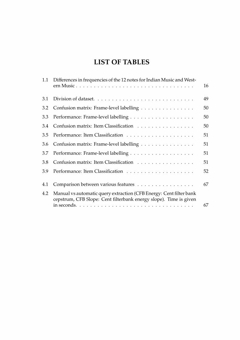
LIST OF TABLES

1.1 Differences in frequencies of the 12 notes for Indian Music and West-ern Music . . . . . . . . . . . . . . . . . . . . . . . . . . . . . . . . . 16

3.1 Division of dataset. . . . . . . . . . . . . . . . . . . . . . . . . . . . 49

3.2 Confusion matrix: Frame-level labelling . . . . . . . . . . . . . . . 50

3.3 Performance: Frame-level labelling . . . . . . . . . . . . . . . . . . 50

3.4 Confusion matrix: Item Classification . . . . . . . . . . . . . . . . 50

3.5 Performance: Item Classification . . . . . . . . . . . . . . . . . . . 51

3.6 Confusion matrix: Frame-level labelling . . . . . . . . . . . . . . . 51

3.7 Performance: Frame-level labelling . . . . . . . . . . . . . . . . . . 51

3.8 Confusion matrix: Item Classification . . . . . . . . . . . . . . . . 51

3.9 Performance: Item Classification . . . . . . . . . . . . . . . . . . . 52

4.1 Comparison between various features . . . . . . . . . . . . . . . . 67

4.2 Manual vs automatic query extraction (CFB Energy: Cent filter bankcepstrum, CFB Slope: Cent filterbank energy slope). Time is givenin seconds. . . . . . . . . . . . . . . . . . . . . . . . . . . . . . . . . 67

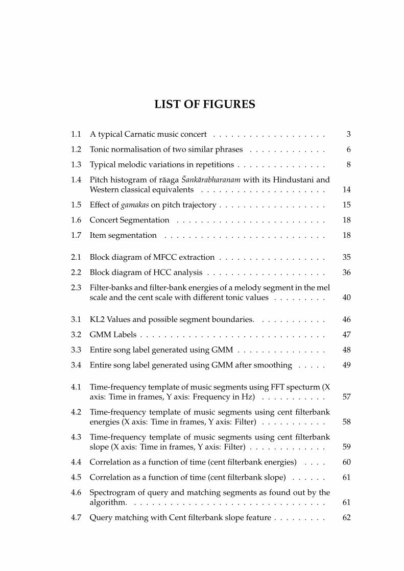
LIST OF FIGURES

1.1 A typical Carnatic music concert . . . . . . . . . . . . . . . . . . . 3

1.2 Tonic normalisation of two similar phrases . . . . . . . . . . . . . 6

1.3 Typical melodic variations in repetitions . . . . . . . . . . . . . . . 8

1.4 Pitch histogram of raaga Sankarabharanam with its Hindustani andWestern classical equivalents . . . . . . . . . . . . . . . . . . . . . 14

1.5 Effect of gamakas on pitch trajectory . . . . . . . . . . . . . . . . . . 15

1.6 Concert Segmentation . . . . . . . . . . . . . . . . . . . . . . . . . 18

1.7 Item segmentation . . . . . . . . . . . . . . . . . . . . . . . . . . . 18

2.1 Block diagram of MFCC extraction . . . . . . . . . . . . . . . . . . 35

2.2 Block diagram of HCC analysis . . . . . . . . . . . . . . . . . . . . 36

2.3 Filter-banks and filter-bank energies of a melody segment in the melscale and the cent scale with different tonic values . . . . . . . . . 40

3.1 KL2 Values and possible segment boundaries. . . . . . . . . . . . 46

3.2 GMM Labels . . . . . . . . . . . . . . . . . . . . . . . . . . . . . . . 47

3.3 Entire song label generated using GMM . . . . . . . . . . . . . . . 48

3.4 Entire song label generated using GMM after smoothing . . . . . 49

4.1 Time-frequency template of music segments using FFT specturm (Xaxis: Time in frames, Y axis: Frequency in Hz) . . . . . . . . . . . 57

4.2 Time-frequency template of music segments using cent filterbankenergies (X axis: Time in frames, Y axis: Filter) . . . . . . . . . . . 58

4.3 Time-frequency template of music segments using cent filterbankslope (X axis: Time in frames, Y axis: Filter) . . . . . . . . . . . . . 59

4.4 Correlation as a function of time (cent filterbank energies) . . . . 60

4.5 Correlation as a function of time (cent filterbank slope) . . . . . . 61

4.6 Spectrogram of query and matching segments as found out by thealgorithm. . . . . . . . . . . . . . . . . . . . . . . . . . . . . . . . . 61

4.7 Query matching with Cent filterbank slope feature . . . . . . . . . 62

4.8 Query matching with Chroma feature (no overlap) . . . . . . . . . 63

4.9 Query matching with Chroma feature (with overlap) . . . . . . . 63

4.10 Query matching with MFCC feature . . . . . . . . . . . . . . . . . 64

4.11 Intermediate output (I) of the automatic query detection algorithmusing slope feature . . . . . . . . . . . . . . . . . . . . . . . . . . . 65

4.12 Intermediate output (II) of the automatic query detection algorithmusing slope feature . . . . . . . . . . . . . . . . . . . . . . . . . . . 66

4.13 Final output of the automatic query detection algorithm using slopefeature. . . . . . . . . . . . . . . . . . . . . . . . . . . . . . . . . . . 66

4.14 Correlation for full query Vs. half query . . . . . . . . . . . . . . . 68

4.15 False positive elimination using rhythmic cycle information . . . 69

4.16 Repeating pattern recognition in other Genres . . . . . . . . . . . 70

4.17 Normal tempo . . . . . . . . . . . . . . . . . . . . . . . . . . . . . . 72

4.18 Half the original tempo . . . . . . . . . . . . . . . . . . . . . . . . . 72

4.19 tisram tempo . . . . . . . . . . . . . . . . . . . . . . . . . . . . . . . 73

4.20 Double the original tempo . . . . . . . . . . . . . . . . . . . . . . . 73

ABBREVIATIONS

AAS Automatic Audio Segmentation

BFCC Bark Filterbank Cepstral Coefficients

BIC Bayesian Information Criteria

CFCC Cent Filterbank Cepstral Coefficients

CNN Convolutional Neural Networks

DCT Discrete Cosine Transform

DFT Discrete Fourier Transform

EM Expectation Maximisation

FFT Fast Fourier Transform

GIR Generalised Likelihood Ratio

GMM Gaussian Mixture Model

HMM Hidden Markov Model

IDFT Inverse Discrete Fourier Transform

KL Divergence KullbackLeibler divergence

LP Linear Prediction

LPCC Linear Prediction Cepstral Coefficients

MFCC Mel Filterbank Cepstral Coefficients

MIR Music Information Retrieval

PSD Power Spectral Density

RMS Root Mean Square

STE Short Term Energy

SVM Support Vector Machine

t-f Time Frequency

ZCR Zero Crossings Rate

CHAPTER 1

Introduction

1.1 Overview of the thesis

Carnatic music is a classical music tradition performed largely in the southern

states of India namely Tamil Nadu, Kerala, Karnataka, Telangana and Andhra

Pradesh. Carnatic music and Hindustani music form the two sub genres of Indian

classical music, the latter being more popular in the Northern states of India.

Though the origin of Carnatic and Hindustani music can be traced back to the

theory of music written by Bharata Muni around 400 BCE, these two sub-genres

have evolved differently over a period of time due to the prevailing socio-political

environments in various parts of India, but still retaining certain core principles in

common. In this work, we will focus mainly on Carnatic music, though some of the

challenges and approaches to MIR described under Carnatic music are applicable

to Hindustani music also.

Raga (melodic modes), tala (repeating rhythmic cycle) and sahitya (lyrics) form

the three pillars on which Carnatic music rests.

The concept of raga is central to Carnatic music. While it can be grossly ap-

proximated to a ‘scale‘ in Western music, in reality a raga encompasses collective

expression of melodic phrases that are formed due to movement or trajectories of

notes that conform to the grammar of that raga. The trajectories themselves are

defined variously by gamakas which are movement, inflexion and ornamentation

of notes [40, Chapter 5]. While a note corresponds to a pitch position in Western

music, a note in Carnatic music (called the svara) need not be a singular pitch

position but a pitch contour or a pitch trajectory as defined by the grammar of that

raga. In other words, a note in Western music corresponds to a point value in a

time- frequency plane while a svara in Carnatic music can correspond to a curve

in the time- frequency plane. The shape of this curve can vary from svara to svara

and raga to raga. The set of svaras that define the raga are dependent on the tonic.

Unlike Western music, the main performer of a concert is at liberty to choose any

frequency as the tonic of that concert. Once a tonic is chosen, the pitch positions

of other notes are derived from the tonic. In a Carnatic music concert, this tonic is

maintained by an instrument called tambura.

The next important concept in Carnatic music is tala. It is related to rhythm,

speed, metre etc and it is a measure of time. There are various types of tala that

are characterised by different matra (beat) count per cycle. The matra is further

subdivided into akshara. The count of akshara per matra is decided by the nadai/gati

of that tala. For every composition, the main artist chooses a speed of the item to

render. Once the speed is chosen, Carnatic music is reasonably strict about keeping

the speed constant, but for inadvertent minor variations in speed due to human

errors.

The third important concept in Carnatic music is sahitya or lyrics. Most of the

lyrical compositions that are performed today have been written a few centuries

ago. The composers were both musicians and poets and hence it can be seen that

music and lyrics go together in their compositions.

A Carnatic music concert is performed by a small ensemble of musicians as

shown in Figure 1.1

2

Figure 1.1: A typical Carnatic music concert

The main artiste is usually a vocalist but an artiste playing flute / veena /

violin can also be a main artiste. Where the main artiste is a vocalist or flautist, the

melodic accompaniment is given by a violin artist. The percussion accompaniment

is always given by a mrudangam artist. An additional percussion accompaniment

in the form of ghatam / khanjira / morsing is optional. A tambura player maintains

the tonic.

A typical Carnatic music concert varies in duration from 90 mins to 3 hours

and is made up of a succession of musical items. These items are standard lyrical

compositions (kritis) with melodies in most cases set to a specific raga and rhythm

structure set to a specific tala. The kritis can be optionally preceded by an alapana

which is the elaboration of the raga.

The main musician chooses a set of musical items that forms the concert. The

choice of items is an important part of concert planning. While there is no hard

and fast rules governing the choice of items, certain traditions are in the vogue

for the past 70 years. There are various musical forms in Carnatic music, namely

3

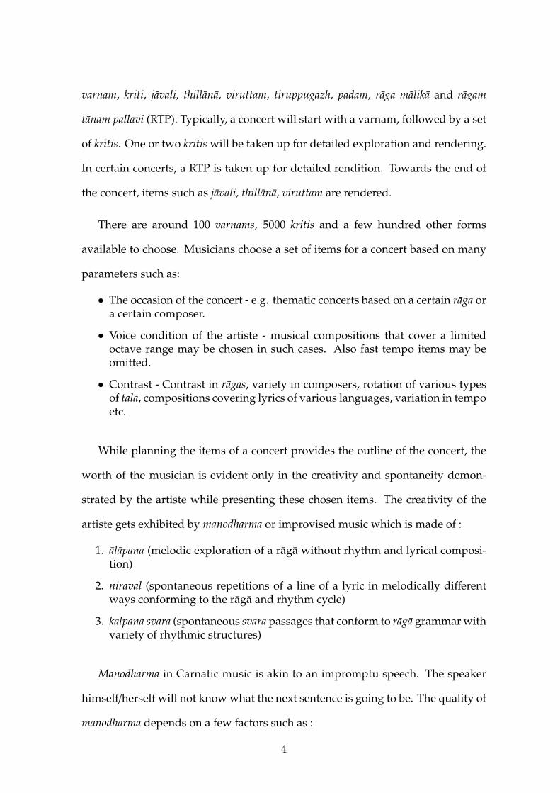
varnam, kriti, javali, thillana, viruttam, tiruppugazh, padam, raga malika and ragam

tanam pallavi (RTP). Typically, a concert will start with a varnam, followed by a set

of kritis. One or two kritis will be taken up for detailed exploration and rendering.

In certain concerts, a RTP is taken up for detailed rendition. Towards the end of

the concert, items such as javali, thillana, viruttam are rendered.

There are around 100 varnams, 5000 kritis and a few hundred other forms

available to choose. Musicians choose a set of items for a concert based on many

parameters such as:

• The occasion of the concert - e.g. thematic concerts based on a certain raga ora certain composer.

• Voice condition of the artiste - musical compositions that cover a limitedoctave range may be chosen in such cases. Also fast tempo items may beomitted.

• Contrast - Contrast in ragas, variety in composers, rotation of various typesof tala, compositions covering lyrics of various languages, variation in tempoetc.

While planning the items of a concert provides the outline of the concert, the

worth of the musician is evident only in the creativity and spontaneity demon-

strated by the artiste while presenting these chosen items. The creativity of the

artiste gets exhibited by manodharma or improvised music which is made of :

1. alapana (melodic exploration of a raga without rhythm and lyrical composi-tion)

2. niraval (spontaneous repetitions of a line of a lyric in melodically differentways conforming to the raga and rhythm cycle)

3. kalpana svara (spontaneous svara passages that conform to raga grammar withvariety of rhythmic structures)

Manodharma in Carnatic music is akin to an impromptu speech. The speaker

himself/herself will not know what the next sentence is going to be. The quality of

manodharma depends on a few factors such as :

4

1. Technical capability of the artiste - A highly accomplished artiste will havethe confidence to take higher risks during improvisations and will be able tocreate attractive melodic and rhythmic patterns on the fly.

2. Technical capability of the co-artists - Since improvisations are not rehearsed,the accompanying artistes have to be on high alert closely following themoves of the main artiste and be ready to do their part of improvisationswhen the main artiste asks them to.

3. The mental and physical condition of the artiste - The artiste may decide notto exert himself/herself too much while traversing higher octaves or fasterrhythmic neravals

4. Audience response and their pulse - If the audience comprises largely ofpeople who do not have deep knowledge, it is prudent not to demonstratetoo much of technical virtuosity.

As we can see, unlike Western classical music, Carnatic music rendition clearly

has two components - the taught / practised / rehearsed part (called kalpita) and

the spontaneous on-the-stage improvisations (manodharma). A MIR system for

Carnatic music should be able to identify / analyse / retrieve information pertain-

ing not only to the kalpita part but also pertaining to the manodharma part. The

unpredictability of the manodharma aspect makes MIR techniques used in Western

classical music ineffective in Carnatcic music.

At this stage, it is reiterated that the notes that make up the melody in Carnatic

music are defined with respect to a reference called tonic frequency. Hence the

analysis of a concert depends on the tonic. This makes MIR of Carnatic music

non trivial. A melody when heard without a reference tonic can be perceived as

a different raga depending on the svara that is assumed as tonic. Two melodic

motifs rendered with two different tonics will not show similarity unless they are

tonic normalised. Figure 1.2 1 shows the pitch contours of two similar melodic

phrases rendered at different tonics. Any time series algorithm will give a high

distance between the two phrases without tonic normalisation. The effect of tonic1Image courtesy Shrey Dutta

5

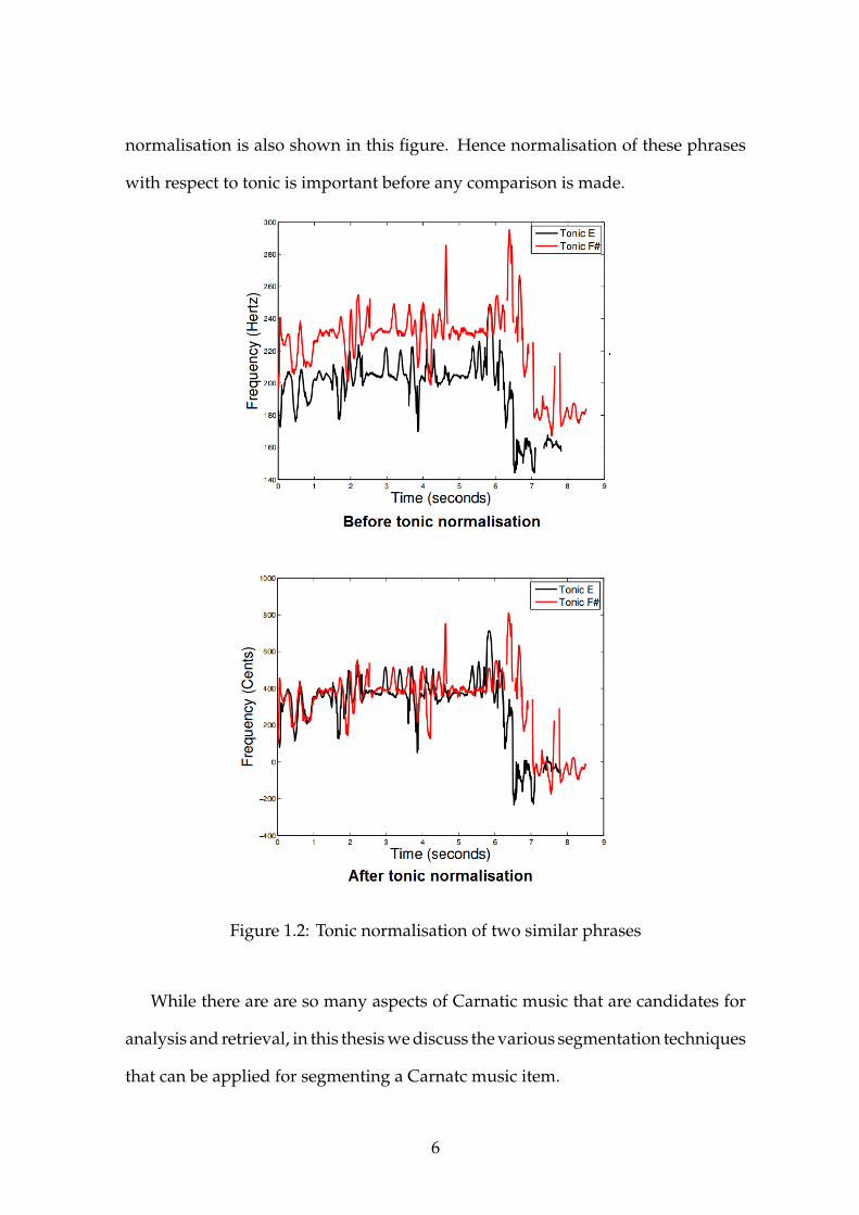
normalisation is also shown in this figure. Hence normalisation of these phrases

with respect to tonic is important before any comparison is made.

Figure 1.2: Tonic normalisation of two similar phrases

While there are are so many aspects of Carnatic music that are candidates for

analysis and retrieval, in this thesis we discuss the various segmentation techniques

that can be applied for segmenting a Carnatc music item.

6

In Carnatic music, a song or composition typically comprises of three segments-

pallavi, anupallavi and caranami-although in some cases there can be more segments.

Segmentation of compositions is important both from the lyrical and musical

aspects, as detailed in chapter 4. The three segments pallavi, anupallavi and caranam

have different significance. From music perspective, one segment builds on the

other. Also, one of the segments is usually taken up for elaboration in the form

of neraval and kalpana svaram. From MIR perspective it is of importance to know

which segment has been taken up by an artiste for elaboration.

The alapana is another creative exercise and the duration of an alapana directly

reflects a musician’s depth of knowledge and creativity. So it is informative to

know the duration of an alapana performed by a main artiste and an accompanying

artist. In this context, segmenting an item into alapana and musical composition if

of interest.

Segmentation of compositions directly from audio is a well researched problem

reported in the literature. Segmentation of a composition into its structural com-

ponents using repeating musical structures (such as chorus) as a cue has several

applications. The segments can be used to index the audio for music summarisa-

tion and browsing the audio (especially when an item is very long). While these

techniques have been attempted for Western music where the repetitions have

more or less static time-frequency melodic content, finding repetitions in impro-

visational music such as Carnatic music is a difficult task. This is because, the

repetitions vary melodically from one repetition to another as illustrated in Figure

1.3. Here the pitch contours of four different repetitions (out of eight rendered) of

the opening line of the composition vatapi are shown.

As we can see, unlike in Western music where segmentation using melodically

7

Figure 1.3: Typical melodic variations in repetitions

invariant chorus is straightforward, segmentation using melodically varying rep-

etitions of pallavi is a non trivial task. In this thesis, we discuss about segmenting

a composition into its constituent parts using pallavi (or a part of pallavi) of the

composition as the query template. As detailed in Chapter 4, the segments of a

composition have lot of melodic and lyrical significance. Hence segmentation of a

composition is a very important MIR task in Carnatic music.

The repeated line of a pallavi is seen as a trajectory in the time-frequency plane.

A sliding window approach is used to determine the locations of the query in the

composition. The locations at which the correlation is maximum corresponds to

matches with the query.

8

We further identify composition segment and the alapana segment using dif-

ference in timbre due to absence of percussion in alapana segment. This done by

evaluating KL2 distance (which is a Information theoretic distance measure be-

tween two probability density functions) between adjacent samples and thereby

locating the boundary of change.

For all these types of segmentations, we use Cent filterbank cepstral coeffi-

cients (CFCC) as features by which the features are tonic independent and hence

comparable across musicians and concerts where variation in tonic is possible.

1.2 Music Information retrieval

There is an ever increasing availability of music in digital format which requires

development of tools for music search, accessing, filtering, classification, visual-

isation and retrieval. Music Information Retrieval (MIR) covers many of these

aspects. Technology for music recording, digitization, and playback allows users

for an access that is almost comparable to the listening of a live performance. Two

main approaches to MIR are common 1) metadata-based and 2) content-based. In

the former, the issue is mainly to find useful categories for describing music. These

categories are expressed in text. Hence, text-based retrieval methods can be used

to search those descriptions. The more challenging approach in MIR is the one

that deals with the actual musical content, e.g. melody and rhythm.

In information retrieval, the objective is to find documents that match a users

information need, as expressed in a query. In content-based MIR, this aim is

usually described as finding music that is similar to a set of features or an example

(query string). There are many different types of musical similarity such as :

9

• Musical works that bring out the same emotion (romantic, sadness etc)

• Musical works that belong to the same genre (ex: classical, jazz etc)

• Musical works created by the same composer

• Music originating from the same culture( etc: Western, Indian)

• Varied repetitions of a melody

In order to perform analyses of various kinds on musical data, it is sometimes

desirable to divide it up into coherent segments. These segmentations can help in

identifying the high-level musical structure of a composition or a concert and can

help in better MIR. Segmentation also helps in creating ”thumbnails” of tracks that

are representative of a composition, thereby enabling surfers to sample parts of

composition before they decide to listen / buy. The identification of musically rele-

vant segments in music requires usage of large amount of contextual information

to assess what distinguishes different segments from each other.

In this work, we focus on segmentation as a tool for MIR in the context of

Carnatic music items.

1.3 Carnatic Music - An overview

The three basic elements of Carnatic music are raga(melody), tala (rhythm) and

sahitya (lyrics).

1.3.1 Raga

Each raga consists of a series of svaras, which bear a definite relationship to the

tonic note (equivalent of key in Western music) and occur in a particular sequence

10

in ascending scale and descending scale. The ragas form the basis of all melody

in Indian Music. The character of each raga is established by the order and the

sequence of notes used in the ascending and descending scales and by the manner

in which the notes are ornamented. These ornamentations, called gamakas, are

subtle, and they are an integral part of the melodic structure. In this respect, raga is

neither a scale, nor a mode. In a concert, ragas can be sung by themselves without

any lyrics (called alapana) and then be followed by a lyrical composition set to tune

in that particular raga. There are finite (72 to be exact) janaka (parent) ragas and

theoretically infinite possible janya (child) ragas born out of these 72 parent ragas.

Ragas are said to evoke moods such as tranquillity, devotion, anger, loneliness,

pathos etc. [42, Page 80] Ragas are also associated with certain time of the day,

though it is not strictly adhered to in Carnatic music.

1.3.2 Tala

Tala or the time measure is another principal element in Carnatic music. Tala is the

rhythmical groupings of beats in repeating cycles that regulates music composi-

tions and provides a basis for rhythmic coordination between the main artistes and

the accompanying artists. Hence, it is the theory of time measure. The beats (called

the matras) are further divided into aksharas. Tala encompasses both structure and

tempo of a rhythmic cycle. Almost all musical compositions other than those sung

as pure ragas (alapana) are set to a tala. There are 108 talas in theory [41, Page 17],

out of which less than 10 are are commonly in practice. Adi tala (8 beat/ cycle) is

the one most commonly used and is also universal. The laya is the tempo, which

keeps the uniformity of time span. In a Carnatic music concert, the tala is shown

with standardized combination of claps and finger counts by the musician.

11

1.3.3 Sahitya

The third important element of Carnatic music is the sahitya (lyrics). A musical

composition presents a concrete picture of not only the raga but the emotions

envisaged by the composer as well. If the composer also happens to be a good

poet, the lyrics are enhanced by the music, while preserving the metre in the lyrics

and the music, leading to an aesthetic experience, where a listener not only enjoys

the music but also the lyrics. The claim of a musical composition to permanence lies

primarily in its musical setting. In compositions considered to be of high quality,

the syllables of the sahitya blends beautifully with the musical setting. Sahitya

serve as the models for the structure of a raga. In rare ragas such as kiranavali

even solitary works of great composer have brought out the nerve-centre of the

raga. The aesthetics of listening to the sound of these words is an integral part

of the Carnatic experience, as the sound of the words blends seamlessly with the

sound of the music. Understanding the actual meanings of the words seems quite

independent of this musical dimension, almost secondary or even peripheral to

the ear that seeks out the music. The words provide a solid yet artistic grounding

and structure to the melody.

1.4 Carnatic Music vs Western Music

While one may be tempted to approach MIR in Carnatic music similar to MIR in

Western music, such attempts are quite likely to fail. There are some fundamental

differences between Western and Indian classical music systems, which are impor-

tant to understand as most of the available techniques on repetition detection and

segmentation for Western music are ineffective for Carnatic music. The differences

12

between these two systems of music are outlined below:

1.4.1 Harmony and Melody

This is the prime difference between the two classical music system. The Western

classical music is primarily polyphonic (i.e) different notes are sounded at the same

time. The concept of western music lies on the ”harmony” created by the different

notes. Thus, we see different instruments sounding different notes being played

at the same time, creating a different feel. It is the principle of ”harmony”. Indian

music system is essentially monophonic, meaning only single note is sung /played

at a time [13, Chapter 1.3]. Its focus is on melodies created using a sequence

of notes. Indian music focusses on expanding those svaras and expounding the

melody aspect, and emotional aspect.

1.4.2 Composed vs improvised

Western music is composed whereas Indian classical music is improvised. All

Western compositions are formally written using the staff notation, and performers

have virtually no latitude for improvisation. The converse is the case with Indian

music, where compositions have been passed on from teacher to student over

generations with improvisations in creative segments such as alapana, niraval and

kalpana svaras on the spot, on the stage.

1.4.3 Semitones, microtones and ornamentations

Western music is largely restricted to 12 semi tones whereas Indian classical music

makes extensive use of 22 microtones (called 22 shrutis though only 12 semi tones

13

are represented formally). In addition to microtones, Indian classical music makes

liberal use of inflexions and oscillations of notes. In Carnatic Music, they are called

gamakas. These gamakas act as ornamentations that describe the contours of a raga.

It is widely accepted that there are ten types of gamakas [45, Page 152]. A svara in

Carnatic music is not a single point of frequency although it is referred to with a

definite pitch value. It is perceived as movements within a range of pitch values

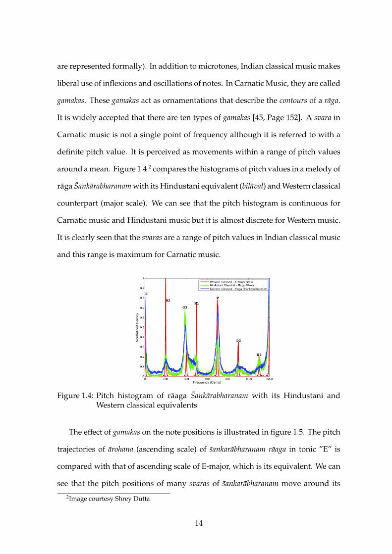
around a mean. Figure 1.4 2 compares the histograms of pitch values in a melody of

raga Sankarabharanam with its Hindustani equivalent (bilaval) and Western classical

counterpart (major scale). We can see that the pitch histogram is continuous for

Carnatic music and Hindustani music but it is almost discrete for Western music.

It is clearly seen that the svaras are a range of pitch values in Indian classical music

and this range is maximum for Carnatic music.

Figure 1.4: Pitch histogram of raaga Sankarabharanam with its Hindustani andWestern classical equivalents

The effect of gamakas on the note positions is illustrated in figure 1.5. The pitch

trajectories of arohana (ascending scale) of sankarabharanam raaga in tonic ”E” is

compared with that of ascending scale of E-major, which is its equivalent. We can

see that the pitch positions of many svaras of sankarabharanam move around its

2Image courtesy Shrey Dutta

14

intended pitch values as the result of ornamentations.

Figure 1.5: Effect of gamakas on pitch trajectory

1.4.4 Notes - absolute vs relative frequencies

In Western music, the positions of the notes are absolute. For instance, middle C is

fixed at 261.6 hz. In Carnatic music, the frequency of the various notes (svaras) are

relative to the tonic note (called Sa or shadjam). Hence the svara ”Sa” may be sung

at C (261.63 Hz) or G (392 Hz) or at any other frequency as chosen by the performer.

The relationship between the notes remains the same in all cases. Hence Ga1 is

always three chromatic steps higher than Sa. Once the key/tonic for the svara Sa is

chosen, then the frequencies for all the other notes are fully determined. There are

also differences in ratios among the 12 notes between Western music and Indian

music as provided in Table 1.1 . In this table, the columns referring to harmonic

are related to Western music. 3.3This Table is courtesy: M V N Murthy, Professor, IMSc

15

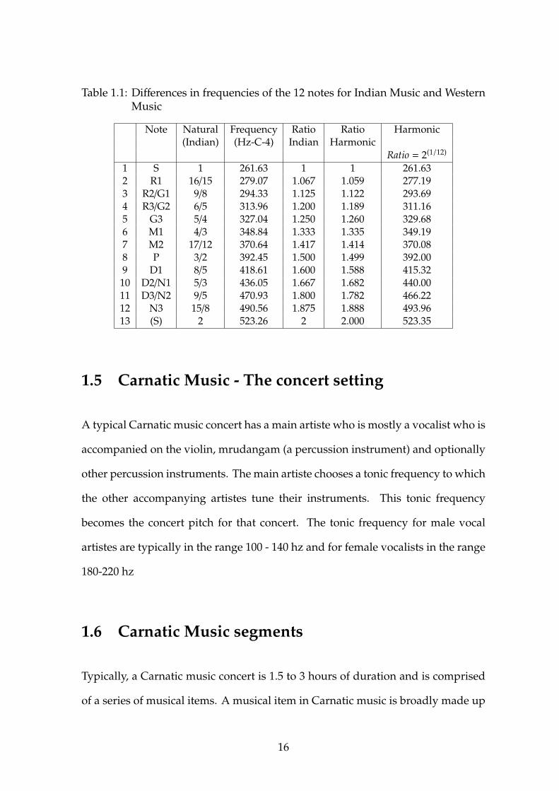
Table 1.1: Differences in frequencies of the 12 notes for Indian Music and WesternMusic

Note Natural Frequency Ratio Ratio Harmonic(Indian) (Hz-C-4) Indian Harmonic

Ratio = 2(1/12)

1 S 1 261.63 1 1 261.632 R1 16/15 279.07 1.067 1.059 277.193 R2/G1 9/8 294.33 1.125 1.122 293.694 R3/G2 6/5 313.96 1.200 1.189 311.165 G3 5/4 327.04 1.250 1.260 329.686 M1 4/3 348.84 1.333 1.335 349.197 M2 17/12 370.64 1.417 1.414 370.088 P 3/2 392.45 1.500 1.499 392.009 D1 8/5 418.61 1.600 1.588 415.32

10 D2/N1 5/3 436.05 1.667 1.682 440.0011 D3/N2 9/5 470.93 1.800 1.782 466.2212 N3 15/8 490.56 1.875 1.888 493.9613 (S) 2 523.26 2 2.000 523.35

1.5 Carnatic Music - The concert setting

A typical Carnatic music concert has a main artiste who is mostly a vocalist who is

accompanied on the violin, mrudangam (a percussion instrument) and optionally

other percussion instruments. The main artiste chooses a tonic frequency to which

the other accompanying artistes tune their instruments. This tonic frequency

becomes the concert pitch for that concert. The tonic frequency for male vocal

artistes are typically in the range 100 - 140 hz and for female vocalists in the range

180-220 hz

1.6 Carnatic Music segments

Typically, a Carnatic music concert is 1.5 to 3 hours of duration and is comprised

of a series of musical items. A musical item in Carnatic music is broadly made up

16

of 2 segments. 1) A composition segment and 2) Optional alapana segment which

precedes the composition segment. These 2 segments can be further segmented as

below:

1.6.1 Composition

The central part of every item is a a song or a composition which is characterised by

participation of all the artistes on the stage. This segment has some lyrics (sahitya)

that is set to a certain melody (raga) and rhythm (tala). Typically this segment

comprises of 3 sub-segments-pallavi, anupallavi and caranam, although in some

cases there can be more segments due to multiple caranam segments. While many

artistes render only one caranam segment (even if the composition has multiple

caranam segments), some artistes do render multiple caranams or all the caranams.

The pallavi part is repeated at the end of anupallavi and caranam.

1.6.2 Alapana

The composition can be optionally preceded by an alapana segment.. If alapana

is present, the percussion instruments do not participate in it. Only the melodic

aspect is expanded and explored without rhythmic support by the main artiste

supported by the violin artist. There are no lyrics for alapana. The main artiste

does the alapana followed by an optional alapana sub-segment by the violin artiste.

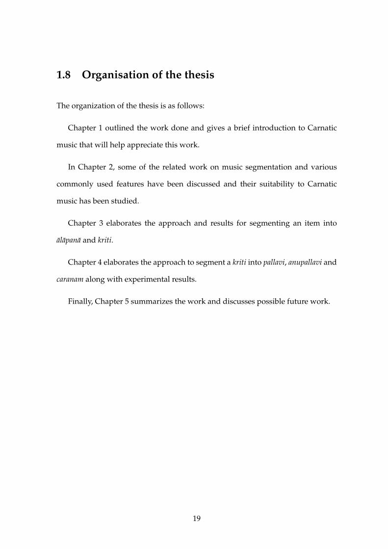
The above description is depicted in the figures 1.6 and 1.7.

17

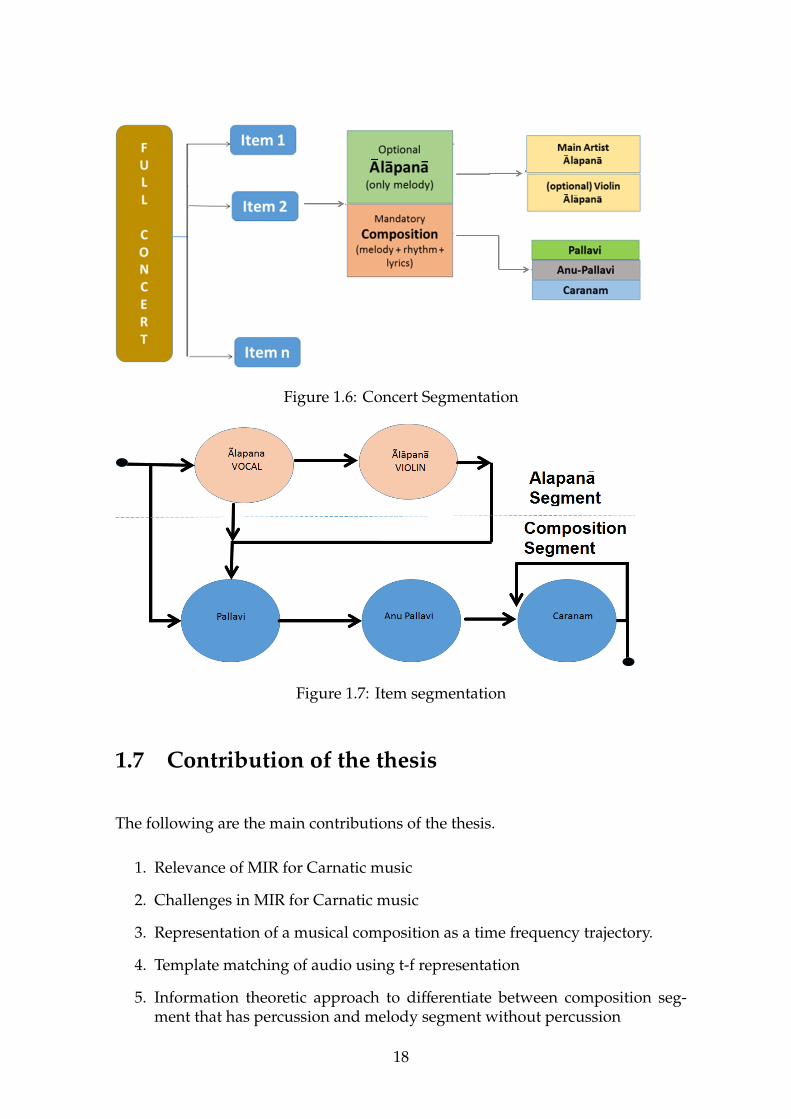
Figure 1.6: Concert Segmentation

Figure 1.7: Item segmentation

1.7 Contribution of the thesis

The following are the main contributions of the thesis.

1. Relevance of MIR for Carnatic music

2. Challenges in MIR for Carnatic music

3. Representation of a musical composition as a time frequency trajectory.

4. Template matching of audio using t-f representation

5. Information theoretic approach to differentiate between composition seg-ment that has percussion and melody segment without percussion

18

1.8 Organisation of the thesis

The organization of the thesis is as follows:

Chapter 1 outlined the work done and gives a brief introduction to Carnatic

music that will help appreciate this work.

In Chapter 2, some of the related work on music segmentation and various

commonly used features have been discussed and their suitability to Carnatic

music has been studied.

Chapter 3 elaborates the approach and results for segmenting an item into

alapana and kriti.

Chapter 4 elaborates the approach to segment a kriti into pallavi, anupallavi and

caranam along with experimental results.

Finally, Chapter 5 summarizes the work and discusses possible future work.

19

CHAPTER 2

Literature Survey

2.1 Introduction

The manner in which humans listen to, interpret and describe music implies that

it must contain an identifiable structure. Musical discourse is structured through

musical forms such as repetitions and contrasts. The forms of the Western music

have been studied in depth by music theorists and codified. Musical forms are

used for pedagogical purposes, in composition as in music analysis and some of

these forms (such as variations or fugues) are also principles of composition.

Musical forms describe how pieces of music are structured. Such forms explain

how the sections/ segments work together through repetition, contrast and vari-

ations. Repetition brings unity, and variation brings novelty and spark interest.

The study of musical forms is fundamental in musical education as among other

benefits, the comprehension of musical structures leads to a better knowledge of

composition rules, and is the essential first approach for a good interpretation of

musical pieces. Every composition in Indian classical music has these forms and

are often an important aspect of what one expects when listening to music.

The terms used to describe that structure varies according to musical genre.

However it is easy for humans to commonly agree upon musical concepts such as

melody, beat, rhythm, repetitions etc. The fact that humans are able to distinguish

between these concepts implies that the same may be learnt by a machine using

signal processing and machine learning. Over the last decade, increase in comput-

ing power and advances in music information retrieval have resulted in algorithms

which can extract features such as timbre [3], [29], [50], tempo and beats [35], note

pitches [26] and chords [32] from polyphonic, mixed source digital music files e.g.

mp3 files, as well as other formats.

Structural segmentation of compositions directly from audio is a well re-

searched problem in the literature, especially for Western music. Automatic audio

segmentation (AAS), is a subfield of Music information retrieval (MIR) that aims

at extracting information on the musical structure of songs in terms of segment

boundaries, repeating structures and appropriate segment labels. With advancing

technology, the explosion of multimedia content in databases, archives and digital

libraries has resulted in new challenges in efficient storage, indexing, retrieval and

management of this content. Under these circumstances, automatic content anal-

ysis and processing of multimedia data becomes more and more important. In

fact, content analysis, particularly content understanding and semantic informa-

tion extraction, have been identified as important steps towards a more efficient

manipulation and retrieval of multimedia content. Automatically extracted struc-

tural information about songs can be useful in various ways, including facilitating

browsing in large digital music collections, music summarisation, creating new

features for audio playback devices (skipping to the boundaries of song segments)

or as a basis for subsequent MIR tasks.

Structural music segmentation consists of dividing a musical piece into several

parts or sections and then assigning to those parts identical or distinct labels

according to their similarity. The founding principles of structural segmentation

are homogeneity, novelty or repetition.

21

Repetition detection is a fundamental requirement for music thumbnailing and

music summarisation. These repetitions are also often the ”chorus” part of a

popular music piece that are thematic and musically uplifting. For these MIR

tasks, a variety of approaches have been discussed in the past.

Previous attempts at music segmentation involved segmenting by spectral

shape, segmenting by harmony, and segmenting by pitch and rhythm. While

these methods exhibited some amount of success, they generally resulted in over

segmentation (identification of segments at locations where segments do not exist).

In this chapter, under section 2.2, we will summarise some of the approaches

attempted by the research community for segmentation and repetition detection

tasks. In section, 2.3, we will review the various audio features commonly used

by speech and music community. We will conclude with our chosen feature and

its suitability for Carnatic music.

2.2 Segmentation Techniques

The authors of [39] discuss three fundamental approaches to music segmenta-

tion - a) novelty-based where transitions are detected between contrasting parts

b) homogeneity-based where sections are identified based on consistency of their

musical properties, and c) repetition-based where recurring patterns are deter-

mined.

In the following subsections, we will do a literature study on the segmentation

approaches carried out using machine learning and other approaches.

22

2.2.1 Machine Learning based approaches

In model-based segmentation approaches used in Machine learning, each audio

frame is separately classified to a specific sound class, e.g. speech vs music, vocal

vs instrumental, melody vs rhythm etc. In particular, a model is used to represent

each sound class. The models for each class of interest are trained using training

data. During the testing (operational) phase, a set of new frames is compared

against each of the models in order to provide decisions (sound labelling) at the

frame-level. Frame labelling is improved using post processing algorithms. Next,

adjacent audio frames labelled with the same sound class are merged to construct

the detected segments. In the model-based approaches the segmentation process is

performed together with the classification of the frames to a set of sound categories.

The most commonly used machine learning algorithms in audio segmentation are

the Gaussian Mixture Model (GMM), Hidden Markov Model (HMM), Support

Vector Machine (SVM) and Artificial Neural Network (ANN).

In [4] a 4-state ergodic HMM is trained with all possible transitions to discover

different regions in music, based on the presence of steady statistical texture fea-

tures. The Baum-Welch algorithm is used to train the HMM. Finally, segmentation

is deduced by interpreting the results from the Viterbi decoding algorithm for the

sequence of feature vectors for the song.

In [30], an automatic segmentation approach is proposed that combines SVM

classification and audio self-similarity segmentation. This approach firstly sep-

arates the sung clips and accompaniment clips from pop music by using SVM

preliminary classification. Next, heuristic rules are used to filter and merge the

classification result to determine potential segment boundaries further. And fi-

23

nally, a self similarity detecting algorithm is introduced to refine segmentation

results in the vicinity of potential points.

In [31], HMM is used as one of the methods to discover song structure. Here

the song is first parameterised using MFCC features. Then these features are used

to discover the song structure either by clustering fixed-length segments or by an

HMM. Finally using this structure, heuristics are used to choose the key phrase.

In [16], techniques such as Wolff-Gibbs algorithm, HMM and prior distribution

are used to segment an audio.

In [38], a fitness function for the sectional form descriptions is used to select

the one with the highest match with the acoustic properties of the input piece. The

features are used to estimate the probability that two segments in the description

are repeats of each other, and the probabilities are used to determine the total fitness

of the description. Since creating the candidate descriptions is a combinatorial

problem a novel greedy algorithm constructing descriptions gradually is proposed

to solve it.

In [1], the audio frames are first classified based on their audio properties,

and then agglomerated to find the homogeneous or self-similar segments. The

classification problem is addressed using an unsupervised Bayesian clustering

model, the parameters of which are estimated using a variant of the EM algorithm.

This is followed by beat tracking, and merging of adjacent frames that might belong

to the same segment.

In [43], segmentation of a full length Carnatic music concert into individual

items using applause as a boundary is attempted. Applauses are identified for

a concert using spectral domain features. GMMs are built for vocal solo, violin

solo and composition ensemble. Audio segments between a pair of the applauses

24

are labeled as vocal solo, violin solo, composition ensemble etc. The composition

segments are located and the pitch histograms are calculated for the composition

segments. Based on similarity measure the composition segment is labelled as

inter-item or intra-item. Based on the inter-item locations, intra-item segments are

merged into the corresponding items

In [48], a Convolutional Neural Networks (CNN) is trained directly on mel-

scaled magnitude spectrograms. The CNN is trained as a binary classifier on

spectrogram excerpts, and it includes a larger input context and respects the higher

inaccuracy and scarcity of segment boundary annotations.

The author(s) of [23] use CNN with spectrograms and self-similarity lag matri-

ces as audio features, thereby capturing more facets of the underlying structural

information. A late time-synchronous fusion of the input features is performed in

the last convolutional layer, which yielded the best results.

2.2.2 Non machine learning approaches

Non machine learning approaches have primarily used time frequency features or

distance measures to identify segment boundaries.

Distance based audio segmentation algorithms estimate segments in the audio

waveform, which correspond to specific acoustic categories, without labelling

the segments with acoustic classes. The chosen audio is blocked into frames,

parametrised, and a metric based on distance is applied to feature vectors that are

adjacent thus estimating what is called a distance curve. The frame boundaries

correspond to peaks of the distance curve where the distance is maximized. These

are positions with high acoustic change, and hence are considered as candidate

25

audio segment boundaries. Post-processing is done on the candidate boundaries

for the purpose of selecting which of the peaks on the distance curve will be

identified as audio segment boundaries. The sequence of segments will not be

classified to a specific audio sound category at this stage. The categorization is

usually performed by a machine learning based classifier as the next stage.

Foote was the first to use a auto-correlation matrix where a song’s frames are

matched against themselves. The author(s) of [18] describe methods for automat-

ically locating points of significant change in music or audio, by analysing local

self-similarity. This approach uses the signal to model itself, and thus does not

rely on particular acoustic cues nor requires training.

This approach was further enhanced in [6], where a self similarity matrix fol-

lowed by dynamic time warping (DTW) was used to find segment transitions and

repetitions.

In [51] unsupervised audio segmentation using Bayesian Information Crite-

rion is used. After identifying the candidate segments using Euclidean distance,

delta-BIC integrating energy-based silence detection is employed to perform the

segmentation decision to pick the final acoustic changes.

In [52], anchor speaker segments are identified using Bayesian Information

Criterion to construct a summary of broadcast news.

In [7], three divide-and-conquer approaches for Bayesian information criterion

based speaker segmentation are proposed. The approaches detect speaker changes

by recursively partitioning a large analysis window into two sub-windows and

recursively verifying the merging of two adjacent audio segments using Delta BIC.

In [9], a two pass approach is used for speaker segmentation. In the first pass,

26

GLR distance is used to detect potential speaker changes, and in second pass, BIC

is used to validate these potential speaker changes.

In [8], the authors describe a system that uses agglomerative clustering in music

structure analysis of a small set of Jazz and Classical pieces. Pitch, which is used

as the feature, is extracted and the notes are identified from the pitch. Using

the sequence of notes, the melodic fragments that repeat are identified using a

similarity measure. Then clusters are formed from pairs of similar phrases and

used to describe the music in terms of structural relationships.

In [17], the authors propose a dissimilarity matrix containing a measure of

dissimilarity for all pairs of feature tuples using MFCC features. The acoustic

similarity between any two instants of an audio recording is calculated and dis-

played as a two-dimensional representation. Similar or repeating elements are

visually distinct, allowing identification of structural and rhythmic characteristics.

Visualization examples are presented for orchestral, jazz, and popular music.

In [21], a feature-space representation of the signal is generated; then, sequences

of feature-space samples are aggregated into clusters corresponding to distinct

signal regions. The clustering of feature sets is improved via linear discriminant

analysis; dynamic programming is used to derive optimal cluster boundaries.

In [22], the authors describe a system called RefraiD that locates repeating

structural segments of a song, namely chorus segments and estimates both ends

of each section. It can also detect modulated chorus sections by introducing a

perceptually motivated acoustic feature and a similarity that enable detection of

a repeated chorus section even after modulation. Chorus extraction is done in

four stages - computation of acoustic features and similarity measures, repeti-

tion judgement criterion, estimating end-points of repeated sections and detecting

27

modulated repetitions

In [33], the structure analysis problem is formulated in the context of spectral

graph theory. By combining local consistency cues with long-term repetition

encodings and analyzing the eigenvectors of the resulting graph Laplacian, a

compact representation is produced that effectively encodes repetition structure at

multiple levels of granularity.

In [46], the authors describe a novel application of the symmetric Kullback-

Leibler distance metric that is used as a solution for segmentation where the

goalis to produce a sequence of discrete utterances with particular characteristics

remaining constant even when speaker and the channel change independently.

In [34], a supervised learning scheme using ordinal linear discriminant analysis

and constrained clustering is used. To facilitate abstraction over multiple training

examples, a latent structural repetition feature is developed, which summarizes the

repetitive structure of a song of any length in a fixed-dimensional representation.

2.3 Audio Features

In machine learning, choosing a feature, which is an individual measurable prop-

erty of a phenomenon is critical. Extracting or selecting features is both an art and

science as it requires experimentation of multiple possible features combined with

domain knowledge. Features are usually numeric and represented by feature vec-

tors. Perception of music is based on the temporal, spectral and spectro-temporal

features. For our work, we could broadly divide the audio features into the fol-

lowing groups :

• Temporal

28

• Spectral

• Cepstral

• Distance based

2.3.1 Temporal Features

Speech and vocal music are produced from a time varying vocal tract system with

time varying excitation. For musical instruments the audio production model is

different from vocal music. Still, the system and the excitation are time variant. As a

result the speech and music signals are non-stationary in nature. Most of the signal

processing approaches studied for signal processing assume time invariant system

and time invariant excitation, i.e. stationary signal. Hence these approaches are

not directly applicable for speech and music processing. While the speech signal

can be considered to be stationary when viewed in blocks of 10-30 msec windows,

music signal can be considered to be stationary when viewed in blocks of 50 - 100

msec windows. Some of the short term parameters are discussed here.

• Short-Time Energy (STE) : The Short-Time Energy of an audio signal is de-fined as

En =

∞∑m=−∞

(x[m])2 w [n −m] (2.1)

where, w [n] is a window function. Normally, a Hamming window is used.

• RMS : The root mean square of the waveform calculated in the time domainto indicate its loudness. It is a measure of amplitude in one analysis windowsand is defined as

RMS =

√x1

2 + x22 + x3

2 + ... + xn2

n

where n is the number of samples within an analysis window and x is thevalue of the sample.

• Zero-Crossing Rate (ZCR): It is defined as the rate at which the signal crosseszero. It is a simple measure of the frequency content of an audio signal. Zero

29

Crossings are also useful to detect the amount of noise in a signal. The ZCRis defined as

Zn =

∞∑m=−∞

| sgn (x[m]) − sgn (x[m − 1]) | w[n −m] (2.2)

where sgn(x[n]) =

{1, x[n] ≥ 0−1, x[n] < 0

where x[n] is a discrete time audio signal, sgn(x[n]) is the signum functionand w [n] is a window function. ZCR can also be used to distinguish betweenvoiced and unvoiced speech signals as unvoiced speech segments normallyhave much higher ZCR values than voiced segments.

• Pitch: Pitch is an auditory sensation in which a listener assigns musicaltones to relative positions on a musical scale based primarily on frequencyof vibration. Pitch, often used interchangeably with fundamental frequency,provides important information about an audio signal that can be used fordifferent tasks including music segmentation [25], speaker recognition [2]and speech analysis and synthesis purposes [47]. Generally, audio signalsare analysed in the time-domain and spectral-domain to characterise a signalin terms of frequency, amplitude, energy etc. But there are some audiocharacteristics such as pitch, which are missing from spectra, which areuseful for characterising a music signal. Spectral characteristics of a signalcan be affected by channel variations, whereas pitch is unaffected by suchvariations. There are different ways to estimate pitch of an audio signal asexplained in [20].

• Autocorrelation: It is the correlation of a signal with a delayed copy of itselfas a function of delay. This is achieved by providing different time lag forthe sequence and computing with the given sequence as reference.

2.3.2 Spectral Features

A temporal signal can be transferred into spectral domain using suitable spectral

transformation, such as the Fourier transform. There are a number of co-efficients

that can be derived from Fast Fourier Transform(FFT) such as :

• Spectral centroid : It indicates a region with the biggest density of frequencyrepresentation in the audio signal. The spectral centroid is commonly associ-ated with the measure of the brightness of a sound. This measure is obtainedby evaluating the center of gravity using the Fourier transforms frequency

30

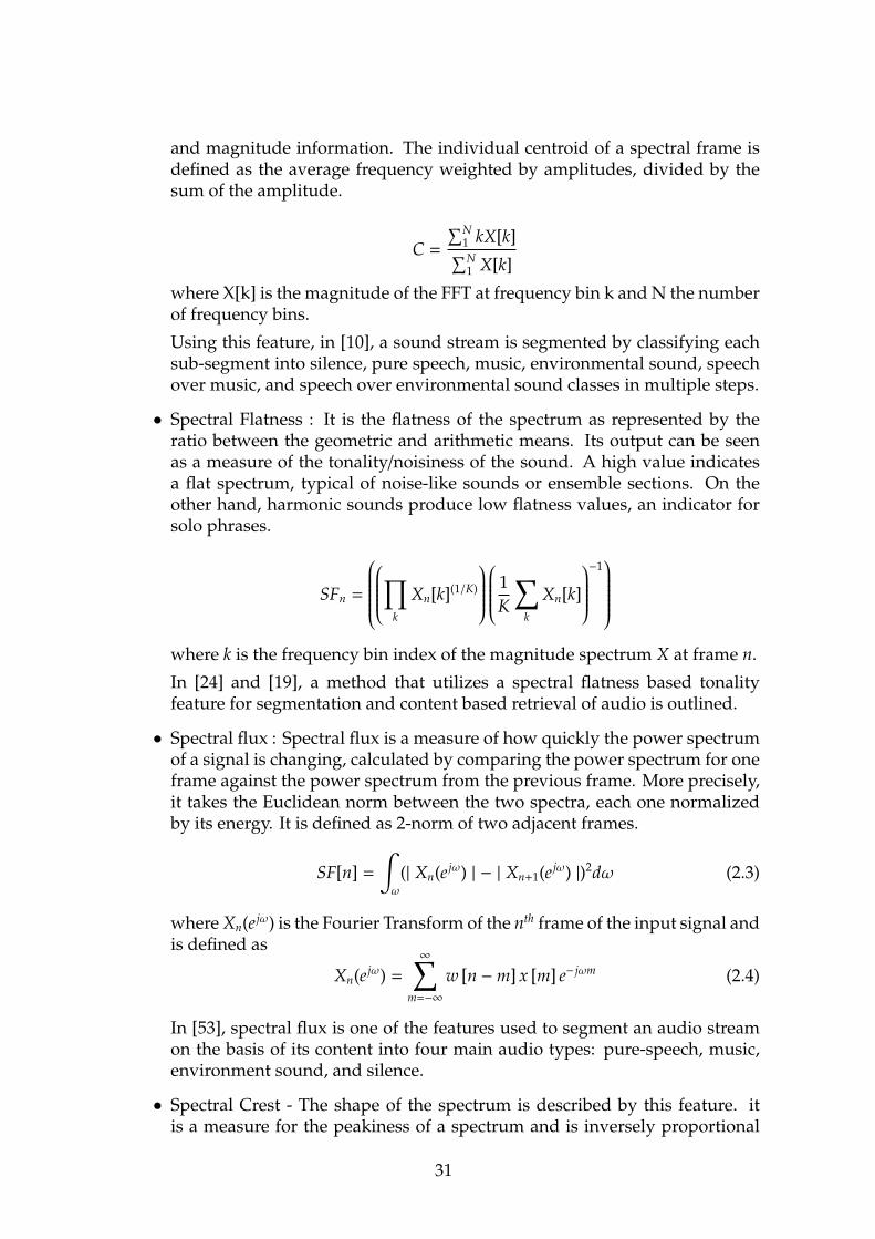
and magnitude information. The individual centroid of a spectral frame isdefined as the average frequency weighted by amplitudes, divided by thesum of the amplitude.

C =

∑N1 kX[k]∑N1 X[k]

where X[k] is the magnitude of the FFT at frequency bin k and N the numberof frequency bins.

Using this feature, in [10], a sound stream is segmented by classifying eachsub-segment into silence, pure speech, music, environmental sound, speechover music, and speech over environmental sound classes in multiple steps.

• Spectral Flatness : It is the flatness of the spectrum as represented by theratio between the geometric and arithmetic means. Its output can be seenas a measure of the tonality/noisiness of the sound. A high value indicatesa flat spectrum, typical of noise-like sounds or ensemble sections. On theother hand, harmonic sounds produce low flatness values, an indicator forsolo phrases.

SFn =

∏

k

Xn[k](1/K)

1

K

∑k

Xn[k]

−1

where k is the frequency bin index of the magnitude spectrum X at frame n.

In [24] and [19], a method that utilizes a spectral flatness based tonalityfeature for segmentation and content based retrieval of audio is outlined.

• Spectral flux : Spectral flux is a measure of how quickly the power spectrumof a signal is changing, calculated by comparing the power spectrum for oneframe against the power spectrum from the previous frame. More precisely,it takes the Euclidean norm between the two spectra, each one normalizedby its energy. It is defined as 2-norm of two adjacent frames.

SF[n] =

∫ω

(| Xn(e jω) | − | Xn+1(e jω) |)2dω (2.3)

where Xn(e jω) is the Fourier Transform of the nth frame of the input signal andis defined as

Xn(e jω) =

∞∑m=−∞

w [n −m] x [m] e− jωm (2.4)

In [53], spectral flux is one of the features used to segment an audio streamon the basis of its content into four main audio types: pure-speech, music,environment sound, and silence.

• Spectral Crest - The shape of the spectrum is described by this feature. itis a measure for the peakiness of a spectrum and is inversely proportional

31

to the spectral flatness. It is used to distinguish between sounds that arenoise-like and tone-like. Noise like spectra will have a spectral crest near 1.It is calculated by the formula

(max(Xn[k])

) 1K

∑k

Xn[k]

−1

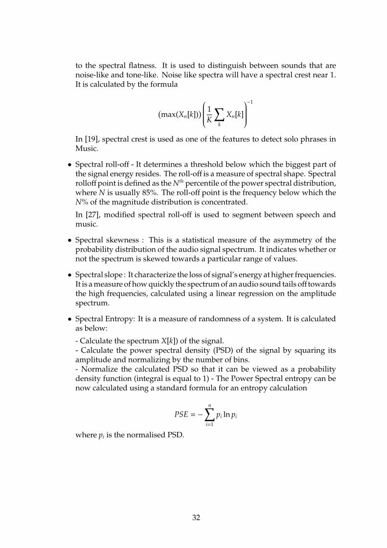
In [19], spectral crest is used as one of the features to detect solo phrases inMusic.

• Spectral roll-off - It determines a threshold below which the biggest part ofthe signal energy resides. The roll-off is a measure of spectral shape. Spectralrolloff point is defined as the Nth percentile of the power spectral distribution,where N is usually 85%. The roll-off point is the frequency below which theN% of the magnitude distribution is concentrated.

In [27], modified spectral roll-off is used to segment between speech andmusic.

• Spectral skewness : This is a statistical measure of the asymmetry of theprobability distribution of the audio signal spectrum. It indicates whether ornot the spectrum is skewed towards a particular range of values.

• Spectral slope : It characterize the loss of signal’s energy at higher frequencies.It is a measure of how quickly the spectrum of an audio sound tails off towardsthe high frequencies, calculated using a linear regression on the amplitudespectrum.

• Spectral Entropy: It is a measure of randomness of a system. It is calculatedas below:

- Calculate the spectrum X[k]) of the signal.- Calculate the power spectral density (PSD) of the signal by squaring itsamplitude and normalizing by the number of bins.- Normalize the calculated PSD so that it can be viewed as a probabilitydensity function (integral is equal to 1) - The Power Spectral entropy can benow calculated using a standard formula for an entropy calculation

PSE = −

n∑i=1

pi ln pi

where pi is the normalised PSD.

32

2.3.3 Cepstral Features

Cepstral analysis originated from speech processing. Speech is composed of two

components - the glottal excitation source and the vocal tract system. These two

components have to be separated from the speech in order to analyze and model

independently. The objective of cepstral analysis is to separate the speech into its

source and system components without any a priori knowledge about source and

/ or system. Because these two component signals are convolved, they cannot be

easily separated in the time domain.

The cepstrum c is defined as the inverse DFT of the log magnitude of the DFT

of the signal x.

c[n] = F −1{log |F {x[n]}|}

where F is the DFT and F −1 is the IDFT.

Cepstral analysis measures rate of change across frequency bands. The cepstral

coefficients are a very compact representation of the spectral envelope. They

are also (to a large extent) uncorrelated. Glottal excitation is captured by the

coefficients where n is high and the vocal tract response, by those where n is

low. For these reasons, cepstral coefficients are widely used in speech recognition,

generally combined with a perceptual auditory scale.

We discuss some types of cepstral coefficients used in speech and music analysis

fields:

• Linear prediction Cepstral co-efficients (LPCC) : For finding the source (glot-tal excitation) and system (vocal tract) components from time domain itself,the linear prediction analysis was proposed by Gunnar Fant [15] as a linearmodel of speech production in which glottis and vocal tract are fully de-coupled. Linear prediction calculates a set of coefficients which provide anestimate - or a prediction - for a forthcoming output sample. The commonest

33

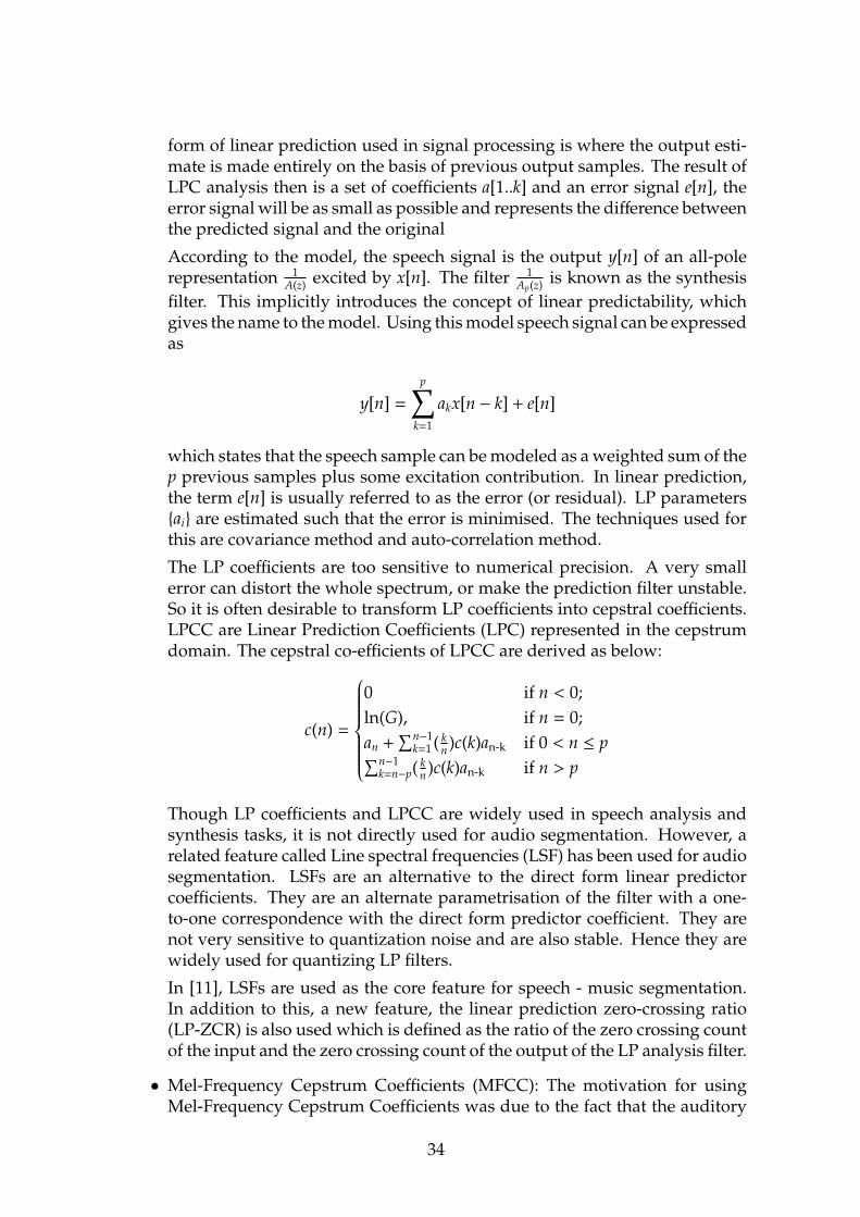
form of linear prediction used in signal processing is where the output esti-mate is made entirely on the basis of previous output samples. The result ofLPC analysis then is a set of coefficients a[1..k] and an error signal e[n], theerror signal will be as small as possible and represents the difference betweenthe predicted signal and the original

According to the model, the speech signal is the output y[n] of an all-polerepresentation 1

A(z) excited by x[n]. The filter 1Ap(z) is known as the synthesis

filter. This implicitly introduces the concept of linear predictability, whichgives the name to the model. Using this model speech signal can be expressedas

y[n] =

p∑k=1

akx[n − k] + e[n]

which states that the speech sample can be modeled as a weighted sum of thep previous samples plus some excitation contribution. In linear prediction,the term e[n] is usually referred to as the error (or residual). LP parameters{ai} are estimated such that the error is minimised. The techniques used forthis are covariance method and auto-correlation method.

The LP coefficients are too sensitive to numerical precision. A very smallerror can distort the whole spectrum, or make the prediction filter unstable.So it is often desirable to transform LP coefficients into cepstral coefficients.LPCC are Linear Prediction Coefficients (LPC) represented in the cepstrumdomain. The cepstral co-efficients of LPCC are derived as below:

c(n) =

0 if n < 0;ln(G), if n = 0;an +

∑n−1k=1 ( k

n )c(k)an-k if 0 < n ≤ p∑n−1k=n−p( k

n )c(k)an-k if n > p

Though LP coefficients and LPCC are widely used in speech analysis andsynthesis tasks, it is not directly used for audio segmentation. However, arelated feature called Line spectral frequencies (LSF) has been used for audiosegmentation. LSFs are an alternative to the direct form linear predictorcoefficients. They are an alternate parametrisation of the filter with a one-to-one correspondence with the direct form predictor coefficient. They arenot very sensitive to quantization noise and are also stable. Hence they arewidely used for quantizing LP filters.

In [11], LSFs are used as the core feature for speech - music segmentation.In addition to this, a new feature, the linear prediction zero-crossing ratio(LP-ZCR) is also used which is defined as the ratio of the zero crossing countof the input and the zero crossing count of the output of the LP analysis filter.

• Mel-Frequency Cepstrum Coefficients (MFCC): The motivation for usingMel-Frequency Cepstrum Coefficients was due to the fact that the auditory

34

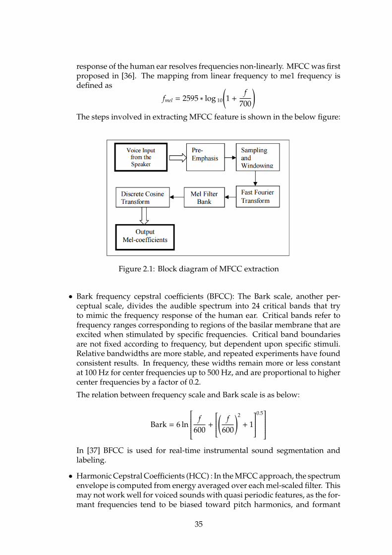
response of the human ear resolves frequencies non-linearly. MFCC was firstproposed in [36]. The mapping from linear frequency to me1 frequency isdefined as

fmel = 2595 ∗ log 10

(1 +

f700

)The steps involved in extracting MFCC feature is shown in the below figure:

Figure 2.1: Block diagram of MFCC extraction

• Bark frequency cepstral coefficients (BFCC): The Bark scale, another per-ceptual scale, divides the audible spectrum into 24 critical bands that tryto mimic the frequency response of the human ear. Critical bands refer tofrequency ranges corresponding to regions of the basilar membrane that areexcited when stimulated by specific frequencies. Critical band boundariesare not fixed according to frequency, but dependent upon specific stimuli.Relative bandwidths are more stable, and repeated experiments have foundconsistent results. In frequency, these widths remain more or less constantat 100 Hz for center frequencies up to 500 Hz, and are proportional to highercenter frequencies by a factor of 0.2.

The relation between frequency scale and Bark scale is as below:

Bark = 6 ln

f600

+

( f600

)2

+ 1

0.5

In [37] BFCC is used for real-time instrumental sound segmentation andlabeling.

• Harmonic Cepstral Coefficients (HCC) : In the MFCC approach, the spectrumenvelope is computed from energy averaged over each mel-scaled filter. Thismay not work well for voiced sounds with quasi periodic features, as the for-mant frequencies tend to be biased toward pitch harmonics, and formant

35

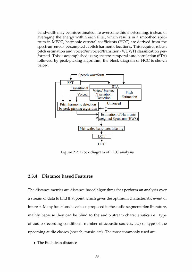
bandwidth may be mis-estimated. To overcome this shortcoming, instead ofaveraging the energy within each filter, which results in a smoothed spec-trum in MFCC, harmonic cepstral coefficients (HCC) are derived from thespectrum envelope sampled at pitch harmonic locations. This requires robustpitch estimation and voiced/unvoiced/transition (V/UV/T) classification per-formed. This is accomplished using spectro-temporal auto-correlation (STA)followed by peak-picking algorithm; the block diagram of HCC is shownbelow:

Figure 2.2: Block diagram of HCC analysis

2.3.4 Distance based Features

The distance metrics are distance-based algorithms that perform an analysis over

a stream of data to find that point which gives the optimum characteristic event of

interest. Many functions have been proposed in the audio segmentation literature,

mainly because they can be blind to the audio stream characteristics i.e. type

of audio (recording conditions, number of acoustic sources, etc) or type of the

upcoming audio classes (speech, music, etc). The most commonly used are:

• The Euclidean distance

36

This is the simplest distance metric for comparing two windows of featurevectors. For distance between two distributions, we take the distance be-tween only the means of the two distributions. For two windows of audiodata described as Gaussian models G1(µ1,Σ1) and (G2(µ2,Σ2), the Euclideandistance metric is given by:

(µ1 − µ2)T(µ1 − µ2)

• The Bayesian information criterion(BIC)

The Bayesian information criterion aims to find the best models that describea set of data. From the two given windows of audio stream the algorithmcomputes three models representing the windows separately and jointly.From each model the formula extracts the likelihood and a complexity termthat expresses the number of the model parameters. For two windows ofaudio data described as Gaussian models G1(µ1,Σ1)and(G2(µ2,Σ2) and withtheir combined windows described as G(µ,Σ) , the ∆BIC distance metric isevaluated as below:

∆BIC = BIC(G1) + BIC(G2) − BIC(G)

BIC(G) = −N log |Σ|

2−λ(d +

d(d−1) log N2 )

2−

dN log 2π2

−N2

∆BIC =N log |Σ|

2−

N1 log |Σ1|

2−

N1 log |Σ2|

2−λd2−λd4

(d+1)(log N1+log N2−log N)

where N,N1,N2 are the number of frames in the corresponding streams, d isthe number of features of the feature vectors andλ is an experimentally factor

In [5], BIC is used detect acoustic change due to speaker change which inturn is used for segmentation based on speaker change.

• The Generalized Likelihood Ratio(GLR): When we process music, context isvery important. We therefore like to understand the trajectory of featuresas a function of time. GLR is a simplification of the Bayesian InformationCriterion. Like BIC, it finds the difference between two windows of audiostream using the three Gaussian models that describe these windows sep-arately and jointly. For two windows of audio data described as Gaussianmodels G1(µ1,Σ1) and G2(µ2,Σ2), the GLR distance is given by:

GLR = w(2 log |Σ] − log[Σ1] − log |Σ2|)

where w is the window size.

In[49], segmenting an audio stream into homogeneous regions accordingto speaker identities, background noise, music, environmental and channelconditions is proposed using GLR.

37

• KL2 Distance Metric based segmentation is a popular technique for seg-mentation. It relies on the computation of a distance between two acousticsegments to determine whether they have similar timbre or not. Change intimbre is an indicator of change in acoustic characteristics such as speaker,musical instrument, background ambience etc.

KL divergence is an information theoretic likelihood-based non-symmetricmeasure that gives the difference between two probability distributions Pand Q. The larger this value, the greater the difference between these PDFs.It is given given by:

DKL(P‖Q) =∑

i

P(i) logP(i)Q(i)

. (2.5)

As mentioned in [46], since DKL(P‖Q) measure is not symmetric, it can notbe used as a distance metric. Hence its variation, KL2 metric is used here fordistance computation. It is defined as follows

DKL2(P,Q) = DKL(P‖Q) + DKL(Q‖P) (2.6)

A Gaussian distribution computed on a window of fourier transformed centnormalised spectrum is considered as a probability density function. KL2distance is computed between adjacent frames to determine the divergencebetween two adjacent spectra.

In [46], KL2 distance is used to detect segment boundaries where speakerchange or channel change occur.

• The Hotelling T2 statistic is another popular tool for comparing distributions.The main difference with KL2 is the assumption that the two comparing win-dows of audio stream have no difference on their covariances. For two win-dows of audio data described as Gaussian models G1(µ1,Σ1) and G2(µ2,Σ2),the Hotelling T2 distance metric is given by:

T2 =N1N2

N1 + N2(µ1 − µ2)TΣ−1(µ1 − µ2)

where Σ equals Σ1 and Σ2 and N1,N2 are the number of frames in the corre-sponding streams

In [54], Hotelling T2 statistic is used to pre-select candidate segmentationboundaries followed by BIC to perform the segmentation decision.

38

2.4 Discussions

While these techniques have been attempted for Western music where the repeti-

tions have more or less static time-frequency melodic content, finding repetitions

in improvisational music is a difficult task. In Indian music, the melody content

of the repetitions varies significantly (Fig 1.3) during repetitions within the same

composition due to the improvisations performed by the musician. A musician‘s

rendering of a composition is considered rich, if (s)he is able improvise and pro-

duce a large number of melodic variants of the line while preserving the grammar,

rhythmic structure and the identity of the composition. Another issue that needs

to be addressed is of the tonic. The same composition when rendered by different

musicians can be sung in different tonics. Hence matching a repeating pattern of a

composition across recordings of various musicians requires a tonic-independent

approach.

The task of segmenting an item into alapana and kriti in Carnatic music involves

differentiating between the textures of the music during alapana and kriti. While

the kriti segment involves both melody and rhythm and hence includes the par-

ticipation of percussion instruments, the alapana segment involves only melody

contributed to by lead performer and the accompanying violinist.

It has been well established in [43] that MFCC features are not suitable for

modelling music analysis tasks where there is a dependency on the tonic. When

MFCCs are used to model music, a common frequency range is used for all musi-

cians, which does not give the best results when variation in tonic is factored in.

With machine learning techniques, when MFCC features are used, training and

testing datasets should have the same tonic. This creates problems when music is

39

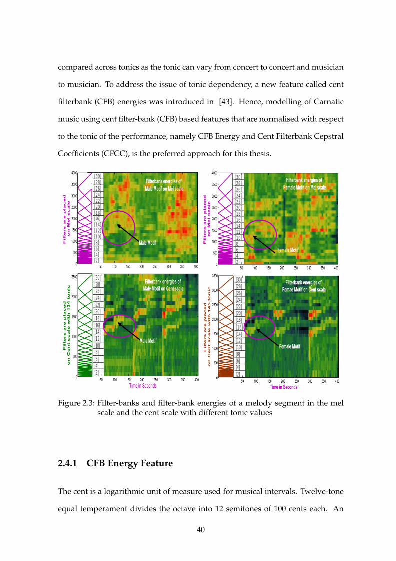
compared across tonics as the tonic can vary from concert to concert and musician

to musician. To address the issue of tonic dependency, a new feature called cent

filterbank (CFB) energies was introduced in [43]. Hence, modelling of Carnatic

music using cent filter-bank (CFB) based features that are normalised with respect

to the tonic of the performance, namely CFB Energy and Cent Filterbank Cepstral

Coefficients (CFCC), is the preferred approach for this thesis.

Figure 2.3: Filter-banks and filter-bank energies of a melody segment in the melscale and the cent scale with different tonic values

2.4.1 CFB Energy Feature

The cent is a logarithmic unit of measure used for musical intervals. Twelve-tone

equal temperament divides the octave into 12 semitones of 100 cents each. An

40

octave (two notes that have a frequency ratio of 2:1) spans twelve semitones and

therefore 1200 cents.

As mentioned earlier, notes that make up a melody in Carnatic music are

defined with respect to the tonic. The tonic chosen for a concert is maintained

throughout the concert using an instrument called the tambura (drone). The anal-

ysis of a concert therefore should depend on the tonic. The tonic ranges from 180

Hz to 220 Hz for female and 100 Hz to 140 Hz for male singers. Tonic normali-

sation in CFB removes the spectral variations. This is illustrated in Fig. 2.3 1 that

shows time filter-bank energy plots for both the mel scale and cent scale. The time

filter-bank energies are shown for the same melody segment as sung by a male

and a female musician. Filter-bank energies and filter-banks are plotted for two

different musicians (male motif with tonic 134 Hz and female motif with tonic 145

Hz) with different tonic values. In the case of mel scale, filters are placed across

the same frequencies for every concert irrespective of the tonic values, whereas, in

the case of the cent scale, the filter-bank frequencies are normalised with respect

to the tonic. The male and female motifs are clearly emphasised irrespective of the

tonic values in the cent scale, and are not clearly emphasised in the mel scale.

CFB energy feature extraction is carried out as below:

1. The audio signal is divided into frames.

2. The short-time DFT is computed for each frame.

3. The frequency scale is normalised by the tonic. The cent scale is defined as:Cent = 1200 . log2 (f / tonic)

4. Six octaves corresponding to [ –1200 : 6000] cents are chosen for every mu-sician. While upto 3 octaves can be covered in a concert, the instrumentsproduce harmonics which are critical to capture the timbre. The choice of sixharmonics is to capture the rich harmonics involved in musical instruments.

1Image courtesy Padi Sarala

41

5. The cent normalised power spectrum is then multiplied by a bank of 80 filtersthat are spaced uniformly in the linear scale to account for the harmonics ofpitch. The choice of 80 filters is based on experimentations in [43].

6. The filterbank energies are computed for every frame and used as a featureafter removing the bias.

CFB energy features were extracted for every frame of length 100 ms of the

musical item, with a shift of 10 ms. Thus, a 80 dimensional feature is obtained for

every 10 ms of the item, resulting in N feature vectors for the entire item.

2.4.2 CFB Slope Feature

In Carnatic music, a collective expression of melodies that consists of svaras (or-

namented notes) in a well defined order constitute phrases (aesthetic threads of

ornamented notes) of a raga. Melodic motifs are those unique phrases of a raga

that collectively give a raga its identity. In Fig. 4.2, it can be seen that the the

presence of the strokes due to the mrudangam destroys the melodic motif. To ad-

dress this issue, cent filterbank based slope was computed along frequency. Let

the vector of log filter bank energy values be represented as Fi = ( f1,i, f2,i, ..., fn f ,i)t,

where n f is the number of filters. Mean subtraction on the sequence Fi, where i =

1,2,..,n is applied as before. Here, n is the number of feature vectors in the query.

To remove the effect of percussion, slope values across consecutive values in each

vector Fi are calculated. Linear regression over 5 consecutive filterbank energies is

performed. A vector of slope values s = (s1,i, s2,i, ..., sF−1,i)t for each frame of music

is obtained as a result.

42

2.4.3 CFCC Feature

To arrive at Cent filterbank cepstral coefficients (CFCC) feature, after carrying out

the steps enumerated in section 2.4.1, DCT is applied on filterbank energies to

de-correlate and the required co-efficients are retained.

43

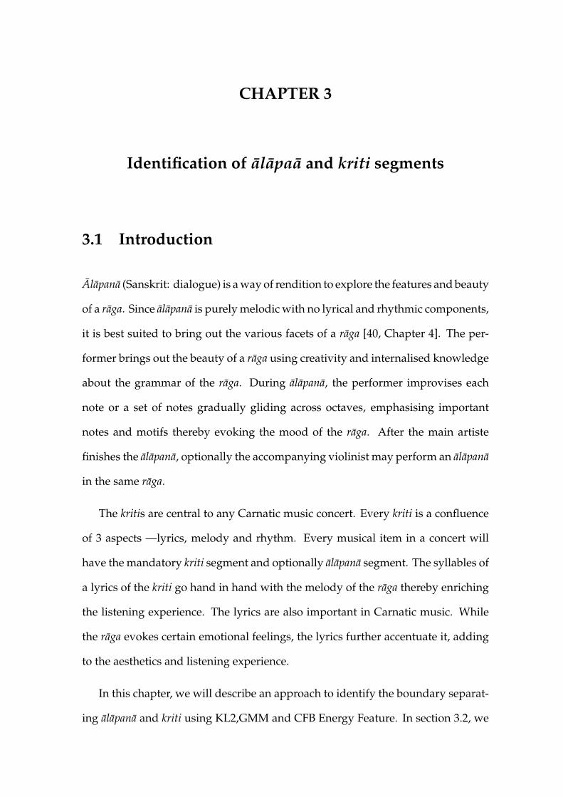
CHAPTER 3

Identification of alapaa and kriti segments

3.1 Introduction

Alapana (Sanskrit: dialogue) is a way of rendition to explore the features and beauty

of a raga. Since alapana is purely melodic with no lyrical and rhythmic components,

it is best suited to bring out the various facets of a raga [40, Chapter 4]. The per-

former brings out the beauty of a raga using creativity and internalised knowledge

about the grammar of the raga. During alapana, the performer improvises each

note or a set of notes gradually gliding across octaves, emphasising important

notes and motifs thereby evoking the mood of the raga. After the main artiste

finishes the alapana, optionally the accompanying violinist may perform an alapana

in the same raga.

The kritis are central to any Carnatic music concert. Every kriti is a confluence

of 3 aspects —lyrics, melody and rhythm. Every musical item in a concert will

have the mandatory kriti segment and optionally alapana segment. The syllables of

a lyrics of the kriti go hand in hand with the melody of the raga thereby enriching

the listening experience. The lyrics are also important in Carnatic music. While

the raga evokes certain emotional feelings, the lyrics further accentuate it, adding

to the aesthetics and listening experience.

In this chapter, we will describe an approach to identify the boundary separat-

ing alapana and kriti using KL2,GMM and CFB Energy Feature. In section 3.2, we

will describe our algorithm used for the segmentation. Under section 3.3, we will

be discussing the results of our experiments. We will conclude this chapter with

discussions on the results.

3.2 Segmentation Approach

3.2.1 Boundary Detection

In order to detect the boundary separating alapana and kriti, individual feature

vectors need to be labelled. One naive approach to find the boundary would be

to label each and every feature vector. Since each feature vector corresponds to 10

ms, and a musical item can last anywhere between 3 mins to 30 mins, there is a

need to label too many feature vectors for the entire musical item. Moreover, there

would be small intervals of time during the kriti, when percussion content would

be absent either due to inter-stroke silence or due to aesthetic pauses deliberately

introduced by the percussionist.

So, a better approach would be to extract a segment of feature vectors from

the item and try to label the segment as a whole. Hence, finding the boundary

between alapana and kriti would involve:

• Iterate over the N feature vectors, one at a time.

• Consider a segment of specified length to the left and right of the currentfeature vector.

• Use a machine learning technique to label these two segment as a whole. Thisreduces the resolution of the segmentation process to the segment length.

• Use music domain knowledge to correct and agglomerate the labels to findthe boundary between alapana and kriti.

45

This approach is computationally intensive. To further improve the efficiency

of this process, we have to reduce the search space for the boundary. The following

approach using KL2 was used:

• Iterate over the N feature vectors, one at a time.

• Consider a sliding window consisting of a sequence of 500 feature vectors (5seconds), Wn, where n denotes the starting position. n = 1, 2..N − 500

• Average the density function obtained earlier for the entire window length.

• Calculate KL2 distance between 2 successive frames of music, Wn and Wn+1.

• Larger values of KL2 distance denote large change in distribution.

• A threshold was automatically chosen such that, there is 3 seconds spacingbetween adjacent peaks of KL2 values. This is to prevent the algorithm fromgenerating too many change points. The choice of 3 seconds was empiricallyarrived at, as a trade-off between accuracy and efficiency.

• The peaks extracted will correspond to a array of K possible boundariesB = [b1, b2, .., bK] between alapana and kriti.

0 1 2 3 4 5 6 7

x 104

0

0.2

0.4

0.6

0.8

1

1.2

1.4

Feature Vector Index

KL

2 V

alu

e

KL2 ValueBoundary PointsAutomatically Chosen ThresholdSelected Peak

Alapana Kriti

Figure 3.1: KL2 Values and possible segment boundaries.

Fig. 3.1 shows the output of the algorithm described above.

46

3.2.2 Boundary verification using GMM

From the K possible boundary values, the actual boundary between kriti and

alapana needs to be identified. In order to verify the boundaries GMMs were

used. GMMs were trained using CFB energy features after applying DCT for

compression. GMMs were trained for both the classes kriti and alapana using a

training dataset with 32 mixtures per class. The approach is as follows:

• A window of length 1000 feature vectors (10 Seconds) was extracted to theleft and right of the possible boundary points, B.

• Labels for left segments, LSL and the right segments, RSL were estimatedusing GMMs (as shown in 3.2).

Figure 3.2: GMM Labels

3.2.3 Label smoothing using Domain Knowledge

Now, using the set of possible boundaries (B) and their left and right segment

labels (LSL and RSL) we need to assign the label for individual feature vector, L.

The following approach was used to find L.

47

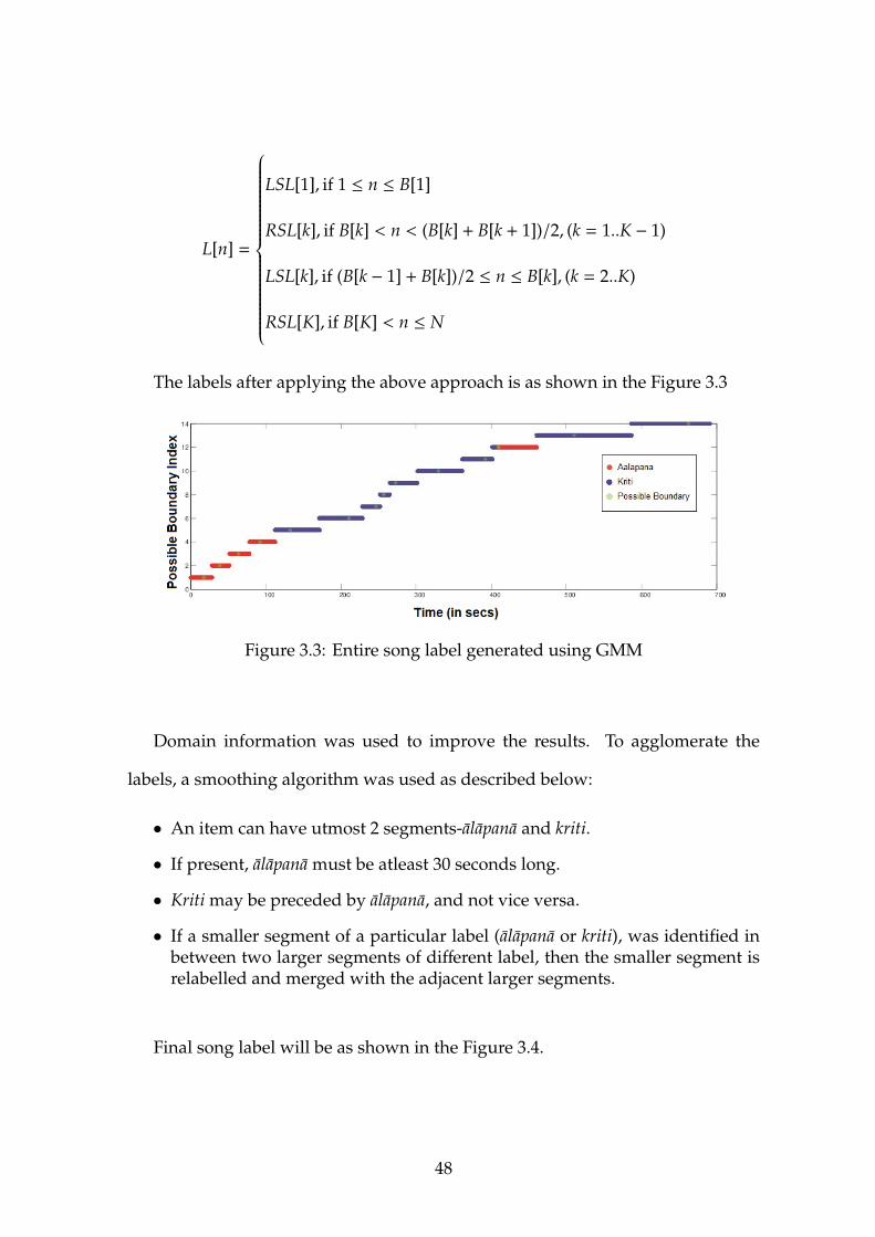
L[n] =

LSL[1], if 1 ≤ n ≤ B[1]

RSL[k], if B[k] < n < (B[k] + B[k + 1])/2, (k = 1..K − 1)

LSL[k], if (B[k − 1] + B[k])/2 ≤ n ≤ B[k], (k = 2..K)

RSL[K], if B[K] < n ≤ N

The labels after applying the above approach is as shown in the Figure 3.3

Figure 3.3: Entire song label generated using GMM

Domain information was used to improve the results. To agglomerate the

labels, a smoothing algorithm was used as described below:

• An item can have utmost 2 segments-alapana and kriti.

• If present, alapana must be atleast 30 seconds long.

• Kriti may be preceded by alapana, and not vice versa.

• If a smaller segment of a particular label (alapana or kriti), was identified inbetween two larger segments of different label, then the smaller segment isrelabelled and merged with the adjacent larger segments.

Final song label will be as shown in the Figure 3.4.

48

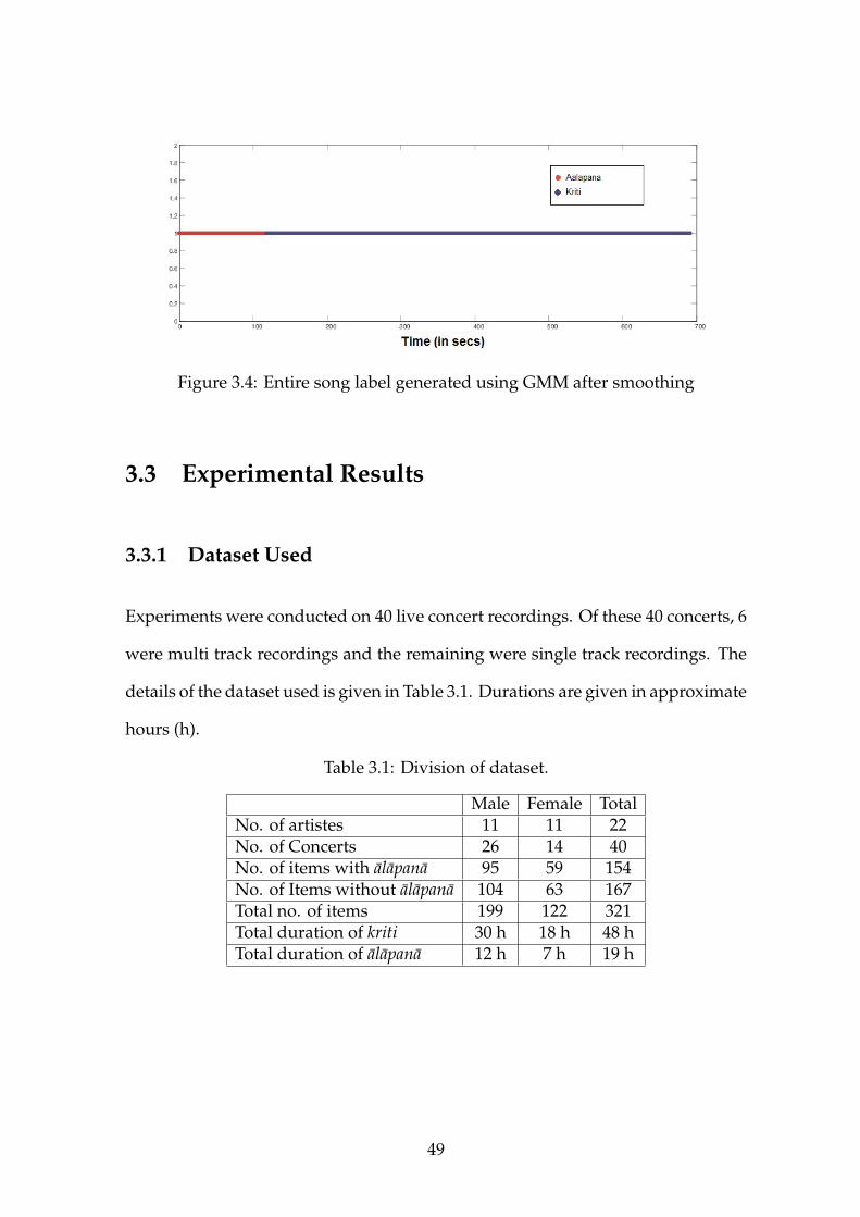
Figure 3.4: Entire song label generated using GMM after smoothing

3.3 Experimental Results

3.3.1 Dataset Used

Experiments were conducted on 40 live concert recordings. Of these 40 concerts, 6

were multi track recordings and the remaining were single track recordings. The

details of the dataset used is given in Table 3.1. Durations are given in approximate

hours (h).

Table 3.1: Division of dataset.

Male Female TotalNo. of artistes 11 11 22No. of Concerts 26 14 40No. of items with alapana 95 59 154No. of Items without alapana 104 63 167Total no. of items 199 122 321Total duration of kriti 30 h 18 h 48 hTotal duration of alapana 12 h 7 h 19 h

49

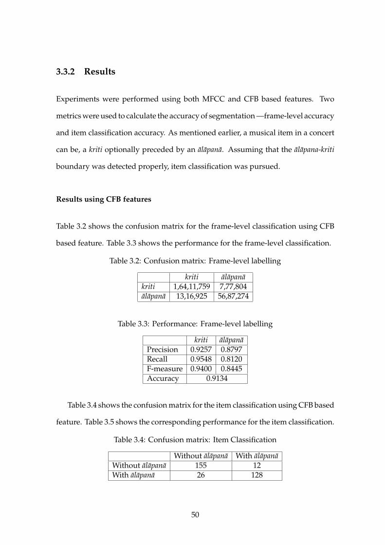
3.3.2 Results

Experiments were performed using both MFCC and CFB based features. Two

metrics were used to calculate the accuracy of segmentation —frame-level accuracy

and item classification accuracy. As mentioned earlier, a musical item in a concert

can be, a kriti optionally preceded by an alapana. Assuming that the alapana-kriti

boundary was detected properly, item classification was pursued.

Results using CFB features

Table 3.2 shows the confusion matrix for the frame-level classification using CFB

based feature. Table 3.3 shows the performance for the frame-level classification.

Table 3.2: Confusion matrix: Frame-level labelling

kriti alapanakriti 1,64,11,759 7,77,804alapana 13,16,925 56,87,274

Table 3.3: Performance: Frame-level labelling

kriti alapanaPrecision 0.9257 0.8797Recall 0.9548 0.8120F-measure 0.9400 0.8445Accuracy 0.9134

Table 3.4 shows the confusion matrix for the item classification using CFB based

feature. Table 3.5 shows the corresponding performance for the item classification.

Table 3.4: Confusion matrix: Item Classification

Without alapana With alapanaWithout alapana 155 12With alapana 26 128

50

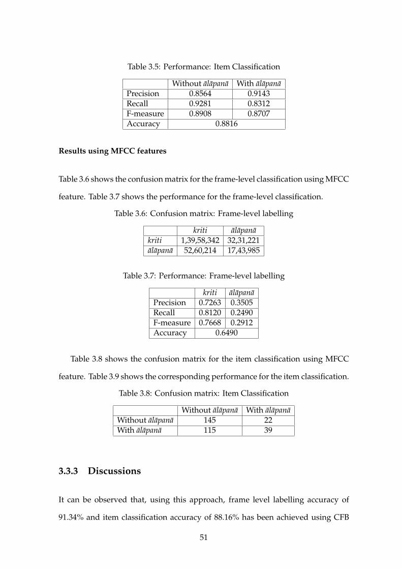
Table 3.5: Performance: Item Classification

Without alapana With alapanaPrecision 0.8564 0.9143Recall 0.9281 0.8312F-measure 0.8908 0.8707Accuracy 0.8816

Results using MFCC features

Table 3.6 shows the confusion matrix for the frame-level classification using MFCC

feature. Table 3.7 shows the performance for the frame-level classification.

Table 3.6: Confusion matrix: Frame-level labelling

kriti alapanakriti 1,39,58,342 32,31,221alapana 52,60,214 17,43,985

Table 3.7: Performance: Frame-level labelling

kriti alapanaPrecision 0.7263 0.3505Recall 0.8120 0.2490F-measure 0.7668 0.2912Accuracy 0.6490

Table 3.8 shows the confusion matrix for the item classification using MFCC

feature. Table 3.9 shows the corresponding performance for the item classification.

Table 3.8: Confusion matrix: Item Classification

Without alapana With alapanaWithout alapana 145 22With alapana 115 39

3.3.3 Discussions

It can be observed that, using this approach, frame level labelling accuracy of

91.34% and item classification accuracy of 88.16% has been achieved using CFB

51

Table 3.9: Performance: Item Classification

Without alapana With alapanaPrecision 0.5577 0.6393Recall 0.8683 0.2532F-measure 0.6792 0.3628Accuracy 0.5732

Energy feature. Whereas using the MFCC feature, frame level labelling accuracy

of 64.90% and item classification accuracy of 57.32 has been achieved. Accuracy of

MFCC is low due to the common frequency range assumed in the feature extraction

process. Also some of the recordings are not clean and in some cases , the alapana

was very short. These have contributed to errors in classification.

52

CHAPTER 4

Segmentation of a kriti

4.1 Introduction

In Carnatic music, a kriti or composition typically comprises of 3 segments-pallavi,

anupallavi and caranam-although in some cases there can be more segments due to

multiple caranam segments. While many artistes render only 1 caranam segment

(even if the composition has multiple caranam segments), some artistes do render

multiple caranam or all the caranams.

The pallavi in a composition in Carnatic music is akin to the chorus or refrain

in Western music albeit with a key difference; the pallavi (or part of it) can be

rendered with a number of variations in melody, without any change in the lyrics,

and is repeated after each segment of a composition. Segmentation and detection of

repeating chorus phrases in Western music is a well researched problem. A number

of techniques have been proposed to segment a Western music composition. While

these techniques have been attempted for Western music where the repetitions

have more or less static time-frequency melodic content, finding repetitions in

improvisational music is a difficult task. In Indian music, the melody content of

the repetitions varies significantly during repetitions within the same composition

due to the improvisations performed by the musician. A musician’s rendering of

a composition is considered rich, if (s)he is able to improvise and produce a large

number of melodic variants of the line while preserving the grammar, identity of

the composition and the raga. Further, the same composition when rendered by

different musicians can be sung in different tonics. Hence matching a repeating

pattern of a composition across recordings of various musicians requires a tonic-

independent approach.

Segmentation of compositions is important both from the perspective of lyrics

and melody. Pallavi, being the first segment, also plays a major role in presenting

a gist of the raga, which gets further elaborated in anupallavi and caranam. In the

pallavi, a musical theme is initiated with key phrases of the raga, developed a

little further in the anupallavi and further enlarged in the caranam, maintaining a

balanced sequence - one built upon the other. Similar stage-by-stage development

from lyrical aspect can also be observed. An idea takes form initially in the

pallavi, which is the central lyrical theme, further emphasised in the anupallavi and

substantiated in the caranam.

Let us illustrate this with an example with the kriti of Saint Tyagaraja. The cen-

tral theme of this composition is ”why there is a screen between us”. The lyrical

meaning of this kriti is as below:

Pallavi: Oh Lord, why this screen (between us) ?

Anu pallavi : Oh lord of moving and non-moving forms who has sun and moon

as eyes, why this screen ?

Caranam: Having searched my inner recess, I have directly perceived that every-

thing is You alone. I shall not even think in my mind of anyone other than You.

Therefore, please protect me. Oh Lord, why this screen ?

The pallavi or a part of pallavi is repeated multiple times with improvisation for

the following reasons: 1) The central lyrical theme that gets expressed in the pallavi

is highlighted by repeating it multiple times, 2) the melodic aspects of the raga

54

and the creative aspects of the artiste (or the music school) jointly get expressed

by repetitions of pallavi. These improvisations in a given composition also stand

out as signatures to identify an artiste or the music school. Since pallavi serves

as a delimiter or separator between the various segments, locating the pallavi

repetitions also leads to knowledge of the number of segments in a composition

(>=3) as rendered by a certain performer.

A commonly observed characteristic of improvisation of pallavi (or a part of it)

is that for a given composition, a portion (typically half) of the repeating segment

will remain more or less constant in melodic content through out the composition

while the other portion varies from one repetition to another. For instance, if

the first half of the repeating segment remains constant in melody, the second half

varies during repetitions and vice-versa. This property is used to locate repetitions

of pallavi inspite of variations in melody from one repetition to another.

In this chapter, under section 4.2, we will discuss the algorithm used to segment

a kriti. Then under section kritiExpResults, we will present the results of our

experiments. We will conclude with discussions on our findings.

4.2 Segmentation Approach

4.2.1 Overview

The structure of a composition in Carnatic music is such that, the pallavi or part of

it gets repeated at the end of anupallavi and caranam segments. Hence our overall

approach is to use the pallavi or a part of it as a query to look for repetitions of

the query in the composition and thereby segment the composition into pallavi ,

55

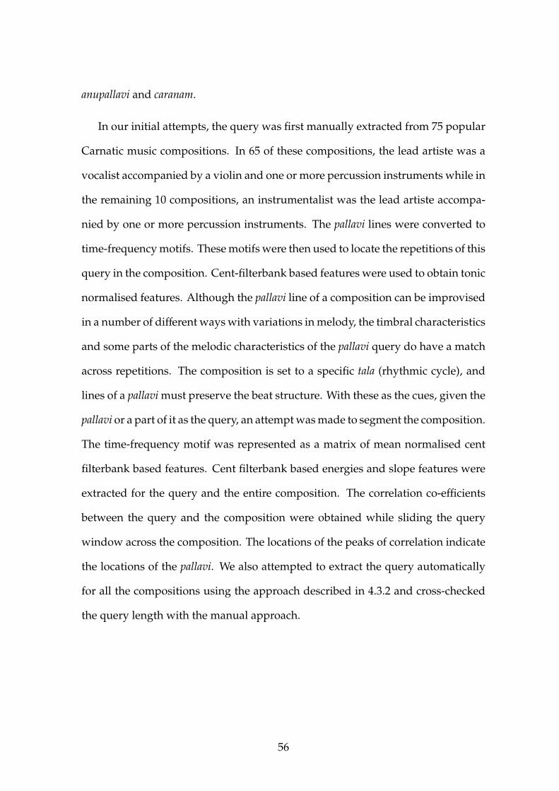
anupallavi and caranam.

In our initial attempts, the query was first manually extracted from 75 popular

Carnatic music compositions. In 65 of these compositions, the lead artiste was a

vocalist accompanied by a violin and one or more percussion instruments while in

the remaining 10 compositions, an instrumentalist was the lead artiste accompa-

nied by one or more percussion instruments. The pallavi lines were converted to

time-frequency motifs. These motifs were then used to locate the repetitions of this

query in the composition. Cent-filterbank based features were used to obtain tonic

normalised features. Although the pallavi line of a composition can be improvised

in a number of different ways with variations in melody, the timbral characteristics

and some parts of the melodic characteristics of the pallavi query do have a match

across repetitions. The composition is set to a specific tala (rhythmic cycle), and

lines of a pallavi must preserve the beat structure. With these as the cues, given the

pallavi or a part of it as the query, an attempt was made to segment the composition.

The time-frequency motif was represented as a matrix of mean normalised cent

filterbank based features. Cent filterbank based energies and slope features were

extracted for the query and the entire composition. The correlation co-efficients

between the query and the composition were obtained while sliding the query

window across the composition. The locations of the peaks of correlation indicate

the locations of the pallavi. We also attempted to extract the query automatically

for all the compositions using the approach described in 4.3.2 and cross-checked

the query length with the manual approach.

56

4.2.2 Time Frequency Templates

The spectrogram is a popular time-frequency representation. The repeated line of

a pallavi is a trajectory in the time-frequency plane. Fig. 4.1 shows spectrograms

of the query and the matched and unmatched time-frequency segments of the

same length in a composition using linear filterbank energies. One can see some

similarity of structure between query and matched segments. Such a similarity

of structure is absent between query and un-matched segments. The frequency

range is set appropriately to occupy about 6 octaves for any musician. Although

the spectrogram does show some structure, the motifs corresponding to that of

the query are not evident. This is primarily because the motif is sung to a specific

tonic. Therefore the analysis of a concert also crucially depends on the tonic.

0

200

400

600

800

1000

0 100 200 300

Query

0

50

100

150

200

250

300

350

0

200

400

600

800

1000

0 100 200 300

Unmatched Segment

50

100

150

200

250

300

350

0

200

400

600

800

1000

0 100 200 300

Unmatched Segment

50

100

150

200

250

300

350

0

200

400

600

800

1000

0 100 200 300

Matched Segment

50

100

150

200

250

300

350

0

200

400

600

800

1000

0 100 200 300

Matched Segment

50

100

150

200

250

300

350

0

200

400

600

800

1000

0 100 200 300

Matched Segment

0

50

100

150

200

250

300

350

Figure 4.1: Time-frequency template of music segments using FFT specturm (Xaxis: Time in frames, Y axis: Frequency in Hz)

57

The cent filterbank energies were computed for both the query and the compo-

sition. The time-dependent filterbank energies were then used as a query. Fig. 4.2

shows a time-frequency template of the query and some matched and unmatched

examples from the composition. A sliding window approach was used to deter-

mine the locations of the query in the composition. The locations at which the

correlation is maximum corresponds to matches with the query. Fig. 4.4 shows

a plot of the correlation as a function of time. The location of the peaks in the

correlation, as verified by a musician, correspond to the locations of the repeating

query.

0

20

40

60

0 100 200 300

Query

-10

-8

-6

-4

-2

0

2

4

0

20

40

60

0 100 200 300

Unmatched

-10

-8

-6

-4

-2

0

2

4

0

20

40

60

0 100 200 300

Unmatched

-10

-8

-6

-4

-2

0

2

4

0

20

40

60

0 100 200 300

Matched

-10

-8

-6

-4

-2

0

2

4

0

20

40

60

0 100 200 300

Matched

-10

-8

-6

-4

-2

0

2

4

0

20

40

60

0 100 200 300

Matched

-10

-8

-6

-4

-2

0

2

4

Figure 4.2: Time-frequency template of music segments using cent filterbank en-ergies (X axis: Time in frames, Y axis: Filter)

As mentioned earlier in 2.4.2, percussion strokes destroy the motif of the

melody. So Cent filterbank slope features were also used as an alternate feature.

Fig. 4.3 shows a plot of the time-dependent query based on filter bank slope and

58

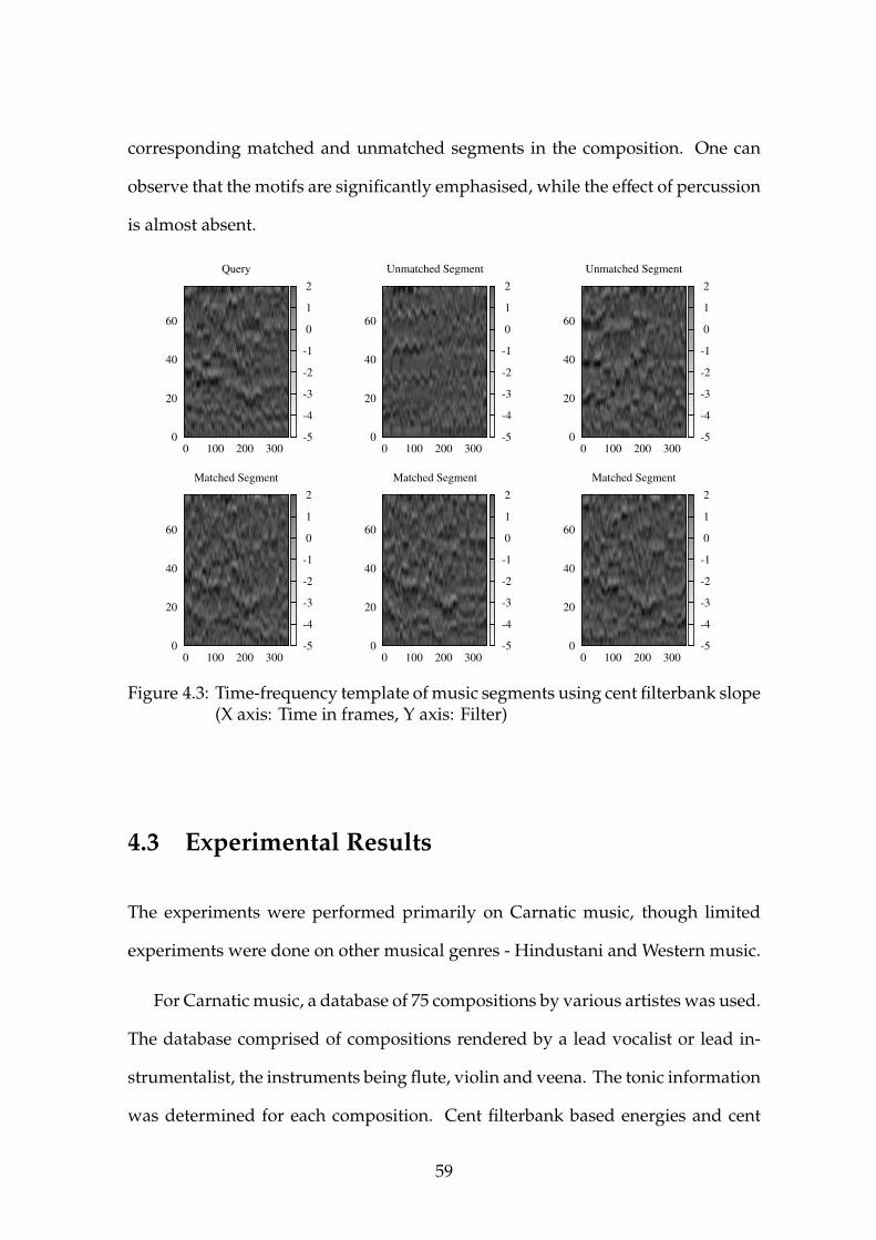
corresponding matched and unmatched segments in the composition. One can

observe that the motifs are significantly emphasised, while the effect of percussion

is almost absent.

0

20

40

60

0 100 200 300

Query

-5

-4

-3

-2

-1

0

1

2

0

20

40

60

0 100 200 300

Unmatched Segment

-5

-4

-3

-2

-1

0

1

2

0

20

40

60

0 100 200 300

Unmatched Segment

-5

-4

-3

-2

-1

0

1

2

0

20

40

60

0 100 200 300

Matched Segment

-5

-4

-3

-2

-1

0

1

2

0

20

40

60

0 100 200 300

Matched Segment

-5

-4

-3

-2

-1

0

1

2

0

20

40

60

0 100 200 300

Matched Segment

-5

-4

-3

-2

-1

0

1

2

Figure 4.3: Time-frequency template of music segments using cent filterbank slope(X axis: Time in frames, Y axis: Filter)

4.3 Experimental Results

The experiments were performed primarily on Carnatic music, though limited

experiments were done on other musical genres - Hindustani and Western music.

For Carnatic music, a database of 75 compositions by various artistes was used.

The database comprised of compositions rendered by a lead vocalist or lead in-

strumentalist, the instruments being flute, violin and veena. The tonic information

was determined for each composition. Cent filterbank based energies and cent

59

filter bank based slope features were extracted for each of these compositions and

used for the experiments. For every 100 millisecond frame of the composition,

80 filters were uniformly placed across 6 octaves (the choice of number of filters

was experimentally arrived at to achieve the required resolution). The correlation

between the query and the moving windows of the composition was computed.

4.3.1 Finding Match with a Given Query

The query for each composition was extracted manually and the cent filterbank

based features were computed. Then Algorithm 1 was used for both CFB based

energy and slope features. Fig. 4.4 and Fig. 4.5 show correlation plots using CFB

energy and slope features for the composition janani ninnu vina. We can see that

the identified repeating patterns clearly stand out among the peaks due to higher

correlation. The spectrogram of the initial portion of the same composition with

the query and the matching sections is shown in Fig. 4.6.

0 50 100 150 200 250 300 350 400−6

−4

−2

0

2

4

6

8

10

12

14x 10

−6

Time (in Seconds)

Correlation

CorrelationThresholdGround Truth

Pallavi

Anu pallavi Caranam

Figure 4.4: Correlation as a function of time (cent filterbank energies)

60

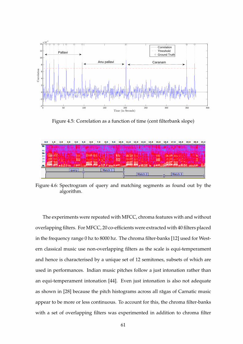
0 50 100 150 200 250 300 350 400−4

−2

0

2

4

6

8

10

12

14x 10

−6

Time (in Seconds)

Correlation

CorrelationThresholdGround Truth

Pallavi

Anu pallavi Caranam

Figure 4.5: Correlation as a function of time (cent filterbank slope)

Figure 4.6: Spectrogram of query and matching segments as found out by thealgorithm.

The experiments were repeated with MFCC, chroma features with and without

overlapping filters. For MFCC, 20 co-efficients were extracted with 40 filters placed

in the frequency range 0 hz to 8000 hz. The chroma filter-banks [12] used for West-

ern classical music use non-overlapping filters as the scale is equi-temperament

and hence is characterised by a unique set of 12 semitones, subsets of which are

used in performances. Indian music pitches follow a just intonation rather than

an equi-temperament intonation [44]. Even just intonation is also not adequate

as shown in [28] because the pitch histograms across all ragas of Carnatic music

appear to be more or less continuous. To account for this, the chroma filter-banks

with a set of overlapping filters was experimented in addition to chroma filter

61

banks without overlapping filters. The comparative performance of these four

features is tabulated in Table 4.1 and the correlation plots for one kriti using these

four features are included in figures 4.7, 4.8, 4.9 and 4.10. It is evident that CFB

based feature outperforms the other three.

Figure 4.7: Query matching with Cent filterbank slope feature

62

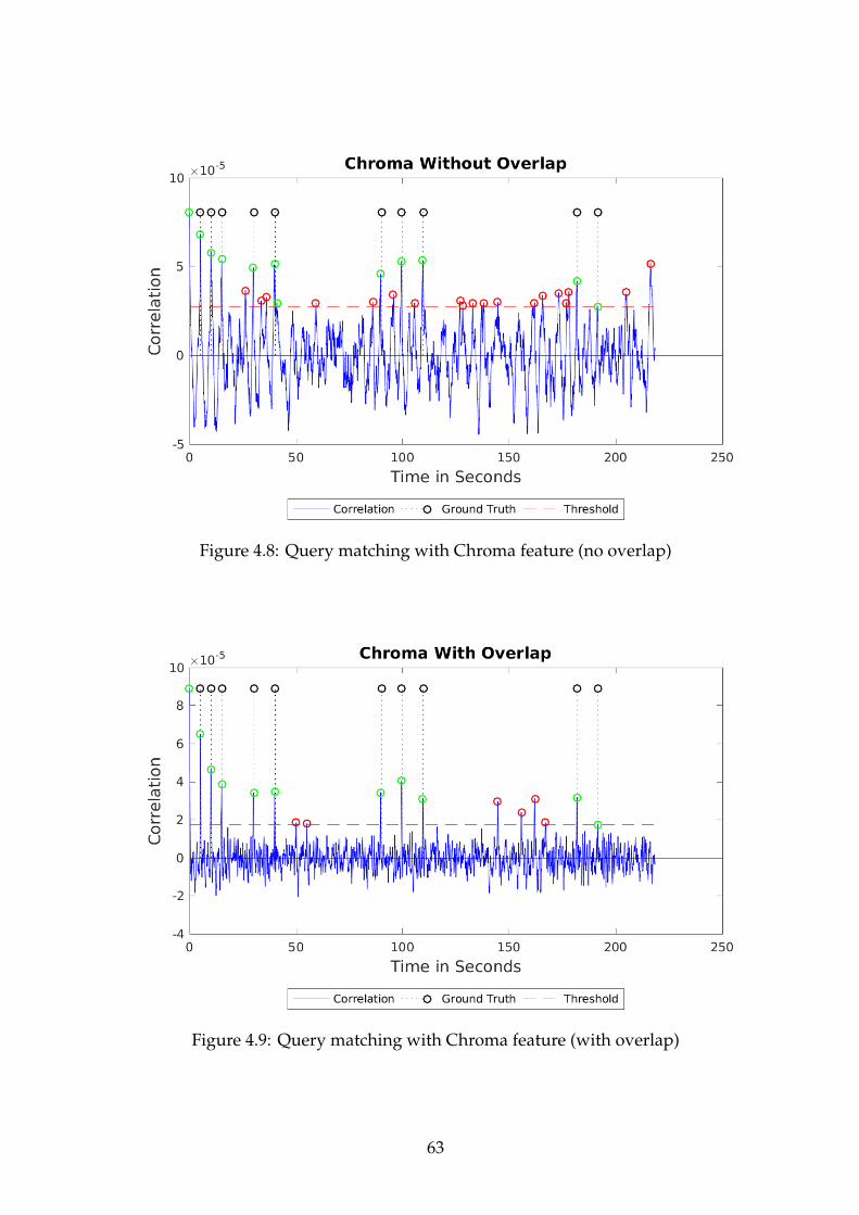
Figure 4.8: Query matching with Chroma feature (no overlap)

Figure 4.9: Query matching with Chroma feature (with overlap)

63

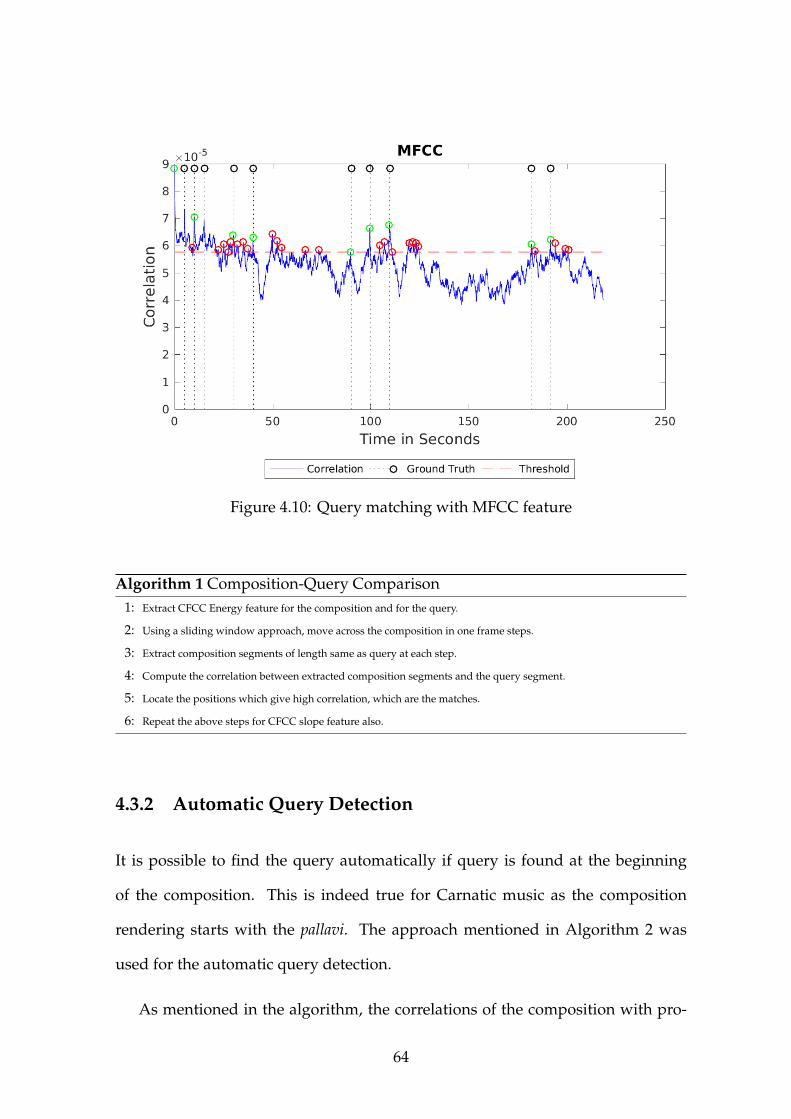
Figure 4.10: Query matching with MFCC feature

Algorithm 1 Composition-Query Comparison1: Extract CFCC Energy feature for the composition and for the query.

2: Using a sliding window approach, move across the composition in one frame steps.

3: Extract composition segments of length same as query at each step.

4: Compute the correlation between extracted composition segments and the query segment.

5: Locate the positions which give high correlation, which are the matches.

6: Repeat the above steps for CFCC slope feature also.

4.3.2 Automatic Query Detection

It is possible to find the query automatically if query is found at the beginning

of the composition. This is indeed true for Carnatic music as the composition

rendering starts with the pallavi. The approach mentioned in Algorithm 2 was

used for the automatic query detection.

As mentioned in the algorithm, the correlations of the composition with pro-

64

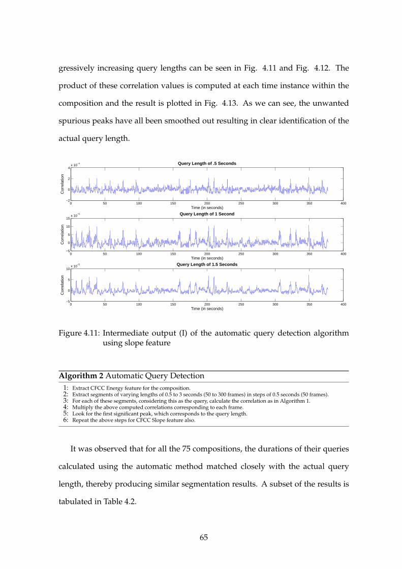
gressively increasing query lengths can be seen in Fig. 4.11 and Fig. 4.12. The

product of these correlation values is computed at each time instance within the

composition and the result is plotted in Fig. 4.13. As we can see, the unwanted

spurious peaks have all been smoothed out resulting in clear identification of the

actual query length.

0 50 100 150 200 250 300 350 400−2

0

2

4x 10

−4 Query Length of .5 Seconds

Time (in seconds)

Cor

rela

tion

0 50 100 150 200 250 300 350 400−5

0

5

10

15x 10

−5 Query Length of 1 Second

Time (in seconds)

Cor

rela

tion

0 50 100 150 200 250 300 350 400−5

0

5

10x 10

−5 Query Length of 1.5 Seconds

Time (in seconds)

Cor

rela

tion

Figure 4.11: Intermediate output (I) of the automatic query detection algorithmusing slope feature

Algorithm 2 Automatic Query Detection1: Extract CFCC Energy feature for the composition.2: Extract segments of varying lengths of 0.5 to 3 seconds (50 to 300 frames) in steps of 0.5 seconds (50 frames).3: For each of these segments, considering this as the query, calculate the correlation as in Algorithm 1.4: Multiply the above computed correlations corresponding to each frame.5: Look for the first significant peak, which corresponds to the query length.6: Repeat the above steps for CFCC Slope feature also.

It was observed that for all the 75 compositions, the durations of their queries

calculated using the automatic method matched closely with the actual query

length, thereby producing similar segmentation results. A subset of the results is

tabulated in Table 4.2.

65

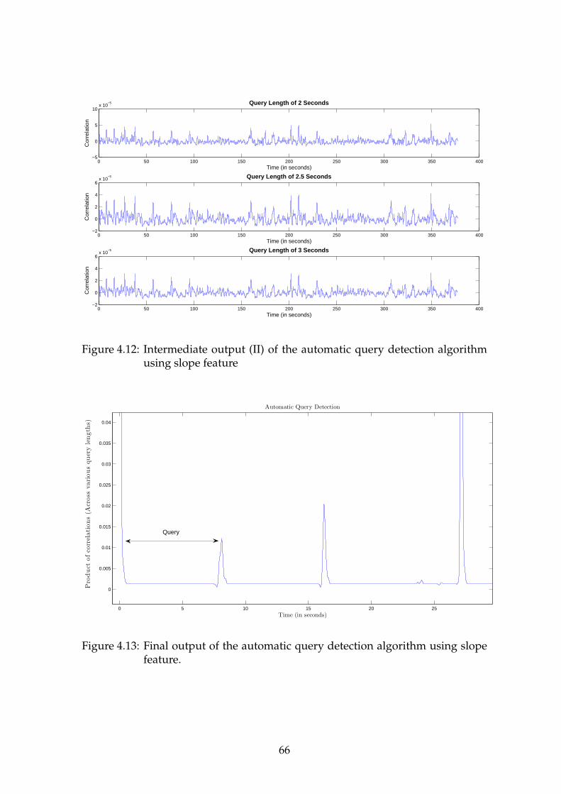
0 50 100 150 200 250 300 350 400−5

0

5

10x 10

−5 Query Length of 2 Seconds

Time (in seconds)

Cor

rela

tion

0 50 100 150 200 250 300 350 400−2

0

2

4

6x 10

−5 Query Length of 2.5 Seconds

Time (in seconds)

Cor

rela

tion

0 50 100 150 200 250 300 350 400−2

0

2

4

6x 10

−5 Query Length of 3 Seconds

Time (in seconds)

Cor

rela

tion

Figure 4.12: Intermediate output (II) of the automatic query detection algorithmusing slope feature

0 5 10 15 20 25

0

0.005

0.01

0.015

0.02

0.025

0.03

0.035

0.04

Time (in seconds)

Product

ofco

rrelations(A

cross

variousquerylength

s)

Automatic Query Detection

Query

Figure 4.13: Final output of the automatic query detection algorithm using slopefeature.

66

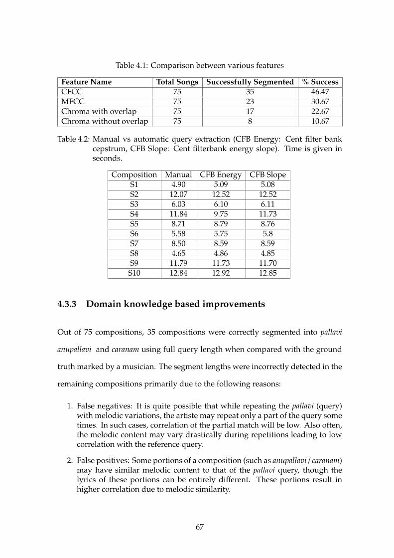
Table 4.1: Comparison between various features

Feature Name Total Songs Successfully Segmented % SuccessCFCC 75 35 46.47MFCC 75 23 30.67Chroma with overlap 75 17 22.67Chroma without overlap 75 8 10.67

Table 4.2: Manual vs automatic query extraction (CFB Energy: Cent filter bankcepstrum, CFB Slope: Cent filterbank energy slope). Time is given inseconds.

Composition Manual CFB Energy CFB SlopeS1 4.90 5.09 5.08S2 12.07 12.52 12.52S3 6.03 6.10 6.11S4 11.84 9.75 11.73S5 8.71 8.79 8.76S6 5.58 5.75 5.8S7 8.50 8.59 8.59S8 4.65 4.86 4.85S9 11.79 11.73 11.70

S10 12.84 12.92 12.85

4.3.3 Domain knowledge based improvements

Out of 75 compositions, 35 compositions were correctly segmented into pallavi

anupallavi and caranam using full query length when compared with the ground

truth marked by a musician. The segment lengths were incorrectly detected in the

remaining compositions primarily due to the following reasons:

1. False negatives: It is quite possible that while repeating the pallavi (query)with melodic variations, the artiste may repeat only a part of the query sometimes. In such cases, correlation of the partial match will be low. Also often,the melodic content may vary drastically during repetitions leading to lowcorrelation with the reference query.

2. False positives: Some portions of a composition (such as anupallavi / caranam)may have similar melodic content to that of the pallavi query, though thelyrics of these portions can be entirely different. These portions result inhigher correlation due to melodic similarity.

67

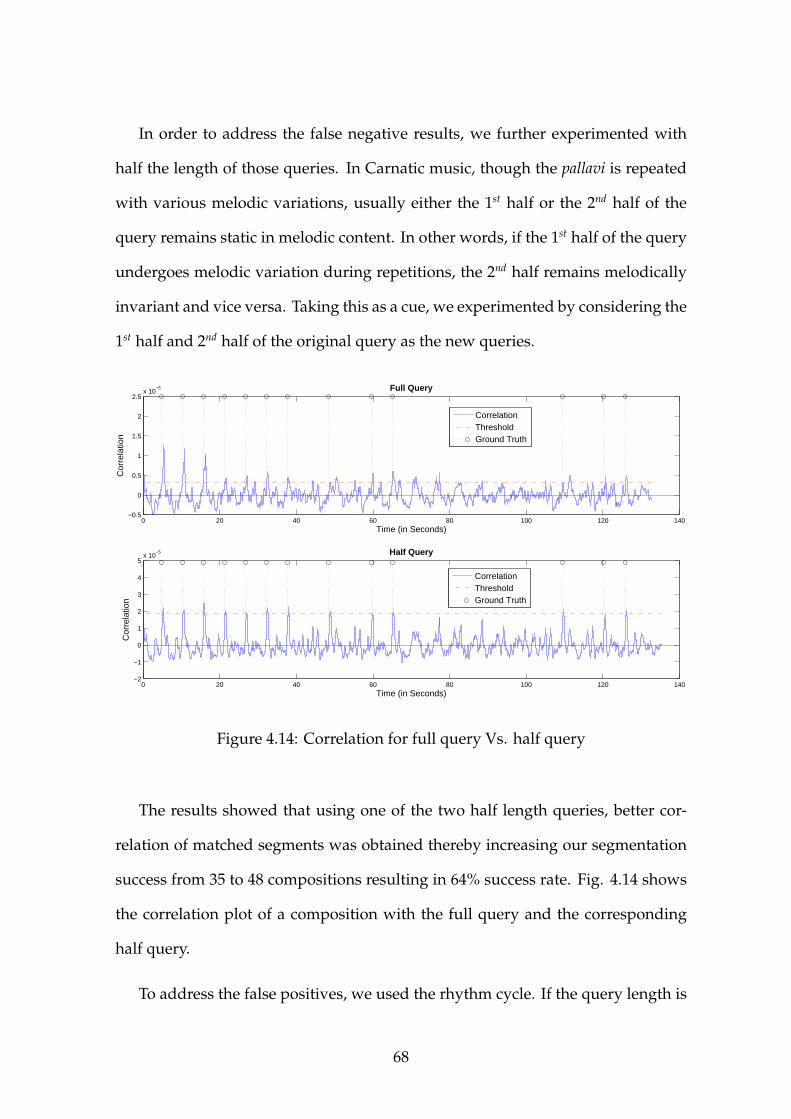
In order to address the false negative results, we further experimented with

half the length of those queries. In Carnatic music, though the pallavi is repeated

with various melodic variations, usually either the 1st half or the 2nd half of the

query remains static in melodic content. In other words, if the 1st half of the query

undergoes melodic variation during repetitions, the 2nd half remains melodically

invariant and vice versa. Taking this as a cue, we experimented by considering the

1st half and 2nd half of the original query as the new queries.

0 20 40 60 80 100 120 140−0.5

0

0.5

1

1.5

2

2.5x 10

−5

Time (in Seconds)

Cor

rela

tion

Full Query

CorrelationThresholdGround Truth

0 20 40 60 80 100 120 140−2

−1

0

1

2

3

4

5x 10

−5

Time (in Seconds)

Cor

rela

tion

Half Query

CorrelationThresholdGround Truth

Figure 4.14: Correlation for full query Vs. half query

The results showed that using one of the two half length queries, better cor-

relation of matched segments was obtained thereby increasing our segmentation

success from 35 to 48 compositions resulting in 64% success rate. Fig. 4.14 shows

the correlation plot of a composition with the full query and the corresponding

half query.

To address the false positives, we used the rhythm cycle. If the query length is

68

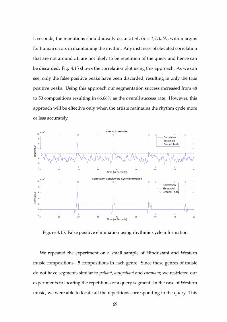
L seconds, the repetitions should ideally occur at nL (n = 1,2,3..N), with margins

for human errors in maintaining the rhythm. Any instances of elevated correlation

that are not around nL are not likely to be repetition of the query and hence can

be discarded. Fig. 4.15 shows the correlation plot using this approach. As we can

see, only the false positive peaks have been discarded, resulting in only the true

positive peaks. Using this approach our segmentation success increased from 48

to 50 compositions resulting in 66.66% as the overall success rate. However, this

approach will be effective only when the artiste maintains the rhythm cycle more

or less accurately.

0 10 20 30 40 50 60 70 80−4

−2

0

2

4

6

8

10x 10

−6

Time (in Seconds)

Cor

rela

tion

Normal Correlation

CorrelationThresholdGround Truth

0 10 20 30 40 50 60 70 80−2

0

2

4

6

8

10x 10

−6

Time (in Seconds)

Cor

rela

tion

Correlation Considering Cycle Information

CorrelationThresholdGround Truth

Figure 4.15: False positive elimination using rhythmic cycle information

We repeated the experiment on a small sample of Hindustani and Western

music compositions - 5 compositions in each genre. Since these genres of music

do not have segments similar to pallavi, anupallavi and caranam; we restricted our

experiments to locating the repetitions of a query segment. In the case of Western

music, we were able to locate all the repetitions corresponding to the query. This

69

is because of little melodic variation between repetitions in Western music. In

the case of Hindustani music, we were able to identify all the repetitions with a

false positive rate of 33%. Fig. 4.16 shows the correlation plot of a Hindustani

composition and a Western music composition.

0 50 100 150 200 250 300−5

0

5

10

15x 10

−6

Time (in Seconds)

Correlation

Hindustani

CorrelationThresholdGround Truth

0 50 100 150 200 250 300−5

0

5

10

15x 10

−6

Time (in Seconds)

Correlation

Western

CorrelationThresholdGround Truth

Figure 4.16: Repeating pattern recognition in other Genres

4.3.4 Repetition detection in a RTP

Ragam Tanam Pallavi (RTP) is a form of singing unique to Carnatic music that

allows the musicians to improvise to a great extent. It incorporates raga alapana,

tanam, niraval, and kalpanasvara and may be followed by a tani avartanam.

Unlike a regular kriti that has pallavi anupallavi and caranam segments, a RTP

has only a pallavi. Also, the pallavi is composed such that it occupies only one

tala cycle. After elaborate alapana and tanam renditions, the pallavi is taken up

for melodic improvisations. This is followed by a rhythmic exercise called tri kala

70

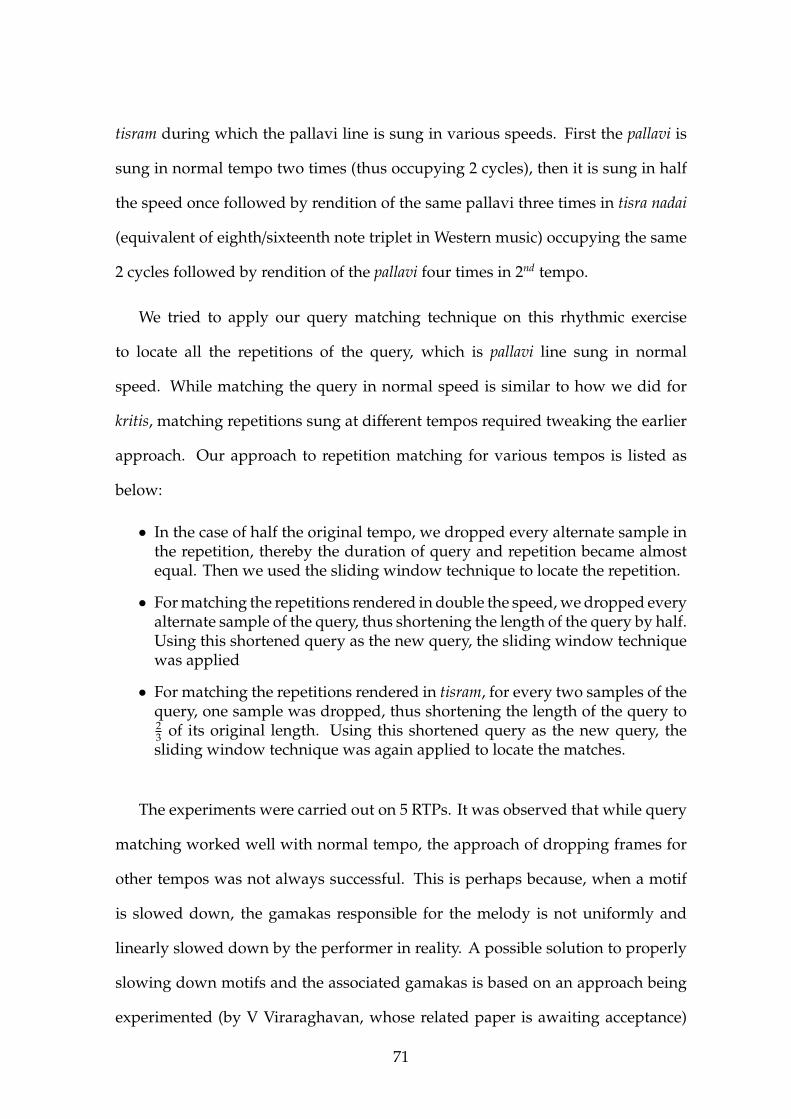
tisram during which the pallavi line is sung in various speeds. First the pallavi is

sung in normal tempo two times (thus occupying 2 cycles), then it is sung in half

the speed once followed by rendition of the same pallavi three times in tisra nadai

(equivalent of eighth/sixteenth note triplet in Western music) occupying the same

2 cycles followed by rendition of the pallavi four times in 2nd tempo.

We tried to apply our query matching technique on this rhythmic exercise

to locate all the repetitions of the query, which is pallavi line sung in normal

speed. While matching the query in normal speed is similar to how we did for

kritis, matching repetitions sung at different tempos required tweaking the earlier

approach. Our approach to repetition matching for various tempos is listed as

below:

• In the case of half the original tempo, we dropped every alternate sample inthe repetition, thereby the duration of query and repetition became almostequal. Then we used the sliding window technique to locate the repetition.

• For matching the repetitions rendered in double the speed, we dropped everyalternate sample of the query, thus shortening the length of the query by half.Using this shortened query as the new query, the sliding window techniquewas applied

• For matching the repetitions rendered in tisram, for every two samples of thequery, one sample was dropped, thus shortening the length of the query to23 of its original length. Using this shortened query as the new query, thesliding window technique was again applied to locate the matches.

The experiments were carried out on 5 RTPs. It was observed that while query

matching worked well with normal tempo, the approach of dropping frames for

other tempos was not always successful. This is perhaps because, when a motif

is slowed down, the gamakas responsible for the melody is not uniformly and

linearly slowed down by the performer in reality. A possible solution to properly

slowing down motifs and the associated gamakas is based on an approach being

experimented (by V Viraraghavan, whose related paper is awaiting acceptance)

71

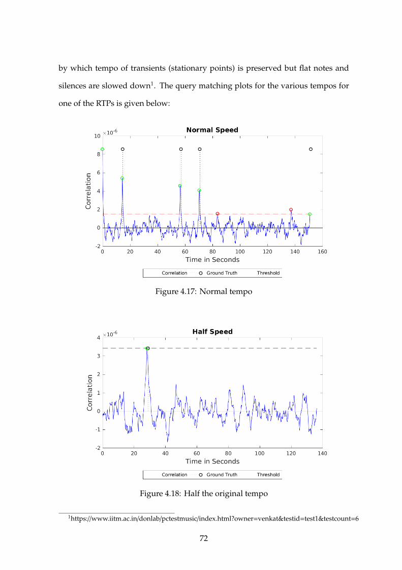
by which tempo of transients (stationary points) is preserved but flat notes and

silences are slowed down1. The query matching plots for the various tempos for

one of the RTPs is given below:

Figure 4.17: Normal tempo

Figure 4.18: Half the original tempo

1https://www.iitm.ac.in/donlab/pctestmusic/index.html?owner=venkat&testid=test1&testcount=6

72

Figure 4.19: tisram tempo

Figure 4.20: Double the original tempo

73

4.3.5 Discussions

For those Carnatic music compositions where segmentation results are accurate, it

is possible to automatically match the audio segments with the pallavi, anupallavi

and caranam lyrics of the composition by looking up a lyrics database. This can

enhance the listening experience by displaying the lyrics as captions when the

composition is played. We were able to automatically generate captions as SRT

(SubRip Text) files for each composition using automatic segmentation and lyrics

database lookup.

It was observed that more the melodic variations of the repetitions, lesser is

the accuracy in segmenting the kriti. While the half query method increased the

accuracy, it can be computationally intense to calculate using full query and then

using both the half queries and choosing the right approach. Cent filter bank

features performed better than mfcc due to tonic normalisation. Though chroma

is tonic normalised, folding of octaves distorted the tf-templates of the motifs and

hence its accuracy was lesser that that of CFB based features. Based on the limited

experiments done with other genres such as Western music and Hindustani music,

we can say that identification of repetitions using t-f template can be extended to

other genres.

74

CHAPTER 5

Conclusion

5.1 Summary of work done

Automatic segmentation of Carnatic music items into segments is required for

automatic archival of a concert for music information retrieval tasks. At present,

there is no automated way to seek directly a given segment within an item. In

this thesis, an attempt was made to segment an item into various segments auto-

matically. A concert is made up of a number of items. Each item can be further

segmented into alapana and kriti and the kriti can be further segmented into pallavi,

anupallavi and caranam.

The key acoustic differentiator between alapaa and kriti is that alapaa is ren-

dered as pure melody without percussion instrument support while kriti is ren-

dered with accompanying percussion instruments. In this thesis, segment bound-

ary between alapaa and kriti was carried out using this key differentiator. Our

approach was to extract a segment of feature vectors from the item and try to

label the segment as a whole. As this approach was computationally intense, to

further improve the efficiency of this process, we had to reduce the search space for

the boundary. We used Kl2 distance metric to look for timbre similarity between

windows. The spectrum of a frame of audio was computed. The spectrum was

converted to a PDF. The KL2 distance was computed between adjacent frames to

determine the divergence between two adjacent spectra. Larger values of KL2

distance denoted large change in distribution. A threshold was automatically

chosen to identify the possible boundaries. Then using domain knowledge, these

boundaries were agglomerated to identify the actual boundary between alapaa

and kriti.

The kriti was further segmented into pallavi, anupallavi an caranam. Our ap-

proach to segmenting a kriti was to use repetition of pallavi as the boundary. In

any kriti, the pallavi gets repeated after anupallavi and again after caranam. By using

pallavi or part of a pallavi¢ as a query, we attempted to look for the repetitions and

hence the segment boundaries. In our initial attempts, the query was fist manually

extracted from 75 popular Carnatic music kritis. We then used time-frequency mo-

tifs to locate the repetitions of this query in the kriti. Cent-filterbank based features

were used to obtain tonic normalised features. Although the pallavi line of a kriti

can be improvised in a number of different ways with variations in melody, the

timbral characteristics and some parts of the melodic characteristics of the pallavi

query do have a match across repetitions. The composition is set to a specific tala

(rhythmic cycle), and lines of a pallavi must preserve the beat structure. With these

as the cues, given the pallavi or a part of it as the query, an attempt was made to

segment the composition. CFB based energies and slope features were extracted

for the query and the entire composition. The correlation co-coefficients between

the query and the kriti were obtained while sliding the query window across the

kriti. The locations of the peaks of correlation indicate the locations of the pallavi.

Next we embarked on identifying the query automatically. It is possible to find

the query automatically if query is found at the beginning of the composition.

This is indeed true for Carnatic music as the composition rendering starts with

the pallavi. It was observed that for all the 75 compositions, the durations of their

queries calculated using the automatic method matched closely with the actual

query length, thereby producing similar segmentation results.

76

We compared the performance of CFB features with that of MFCC and chroma

features. It was found that CFB features outperformed MFCC and chroma features,

justifying our choice of features.

5.2 Criticism of the work

Currently, for segmenting a kriti¢, threshold setting for peak picking is done man-

ually. This manual intervention should be addressed in the future work.

Automatic query detection algorithm works only if the query is exactly at the

start of the item. It is possible that there can be some gap or drone sound at

the beginning. In such cases automatic query detection will fail. This has to be

addressed

Currently locating boundary between alapana and kriti is computational inten-

sive. Tradeoff has to be made between accuracy and performance.

Pallavi repetition detection in RTPs was not giving consistent results for slower

and faster tempos of rendition of the pallavi line. Dropping of samples to increase

the speed of audio appears to spoil the motif and the embedded gamakas and hence

alternate approaches to preserve the shape of the gamaka to be explored.

5.3 Future work

In this work, we have presented a novel approach to composition segmentation

using cent filterbank based features. This approach is particularly suited for Car-

natic music as compared to other fingerprinting algorithms. In Indian music, the

same composition can be sung in different tonics. Further, a number of different

77

variants of the pallavi can be sung. This can vary from musician to musician and

the position of the composition in the entire concert. A large number of variations

is an indication that the musician has chosen the particular composition for a more

detailed exploration.

This segmentation work of the composition into pallavi, anupallavi and caranam

using the repeating pallavi line can be extended to locate repeating niraval patterns

and kalpana-svara portions of an item.

Knowledge of intra kriti segment boundary locations can also be used to look

up lyric database and display the lyrics of those segments as captions when the

music is played. Since lyrics play a pivotal role in Carnatic music, such an effort

will enhance the pleasure of listening to music.

While we have identified the boundary between alapana and kriti, it is possible

to take up identification of the boundary between vocal alapaa and violin alapaa

to further sub-segment the alapaa segment.

The main musical item of a concert will usually feature a thaniavarthanam

during which only the percussion instruments play pure rhythmic patterns. Future

work can take up identification of thaniavarthanam portion in a main item. This

will be of immense value to students of percussion music and rhythm enthusiasts.

78

REFERENCES

[1] Samer Abdallah, Katy Noland, Mark Sandler, Michael A Casey, Christophe Rhodes,et al. Theory and evaluation of a bayesian music structure extractor. 2005.

[2] Bishnu Saroop Atal. Automatic speaker recognition based on pitch contours. TheJournal of the Acoustical Society of America, 52(6B):1687–1697, 1972.

[3] J. Aucouturier, F. Pachet, and M. Sandler. The way it sounds:timbre models foranalysis and retrieval of music signals. In IEEE Trans. Multimedia, vol. 7, no. 6, pp1028–1035, 2005.

[4] Jean-Julien Aucouturier and Mark Sandler. Segmentation of musical signals usinghidden markov models. Preprints-Audio Engineering Society, 2001.

[5] Messaoud Bengherabi and A Sehad. Development and evaluation of automatic-speaker based-audio identification and segmentation for broadcast news recordingsindexation. In Information and Communication Technologies, 2006. ICTTA’06. 2nd, vol-ume 1, pages 1230–1235. IEEE, 2006.

[6] Wei Chai. Automated analysis of musical structure. PhD thesis, Massachusetts Instituteof Technology, 2005.

[7] Shih-Sian Cheng, Hsin-Min Wang, and Hsin-Chia Fu. Bic-based audio segmentationby divide-and-conquer. In 2008 IEEE International Conference on Acoustics, Speech andSignal Processing, pages 4841–4844. IEEE, 2008.

[8] Roger B Dannenberg and Ning Hu. Discovering musical structure in audio recordings.In Music and Artificial Intelligence, pages 43–57. Springer, 2002.

[9] Charlet Delphine. Model-free anchor speaker turn detection for automatic chaptergeneration in broadcast news. In ICASSP, pages 4966–4969, 2010.

[10] Ebru Dogan, Mustafa Sert, and Adnan Yazici. Content-based classification and seg-mentation of mixed-type audio by using mpeg-7 features. In Advances in Multimedia,2009. MMEDIA’09. First International Conference on, pages 152–157. IEEE, 2009.

[11] Khaled El-Maleh, Mark Klein, Grace Petrucci, and Peter Kabal. Speech/music dis-crimination for multimedia applications. In Acoustics, Speech, and Signal Processing,2000. ICASSP’00. Proceedings. 2000 IEEE International Conference on, volume 4, pages2445–2448. IEEE, 2000.

[12] Daniel PW Ellis. Classifying music audio with timbral and chroma features. In ISMIR,volume 7, pages 339–340, 2007.

[13] Asoke Kumar et al. Signal analysis of hindustani classical music, springer 2017.

[14] Universitat Pompeu Fabra. Computational models for the discovery of the world’smusic. http://compmusic.upf.edu/node/25.

79

[15] Gunnar Fant. Acoustic theory of speech production: with calculations based on X-ray studiesof Russian articulations, volume 2. Walter de Gruyter, 1971.

[16] Paul Finkelstein. Music segmentation using markov chain methods. 2011.

[17] Jonathan Foote. Visualizing music and audio using self-similarity. In Proceedings of theseventh ACM international conference on Multimedia (Part 1), pages 77–80. ACM, 1999.

[18] Jonathan Foote. Automatic audio segmentation using a measure of audio novelty. InMultimedia and Expo, 2000. ICME 2000. 2000 IEEE International Conference on, volume 1,pages 452–455. IEEE, 2000.

[19] Ferdinand Fuhrmann, Perfecto Herrera, and Xavier Serra. Detecting solo phrasesin music using spectral and pitch-related descriptors. Journal of New Music Research,38(4):343–356, 2009.

[20] David Gerhard. Pitch extraction and fundamental frequency: History and current tech-niques. Regina: Department of Computer Science, University of Regina, 2003.

[21] Michael M Goodwin and Jean Laroche. Audio segmentation by feature-space cluster-ing using linear discriminant analysis and dynamic programming. In Applications ofSignal Processing to Audio and Acoustics, 2003 IEEE Workshop on., pages 131–134. IEEE,2003.

[22] Masataka Goto. A chorus-section detecting method for musical audio signals. InAcoustics, Speech, and Signal Processing, 2003. Proceedings.(ICASSP’03). 2003 IEEE In-ternational Conference on, volume 5, pages V–437. IEEE, 2003.

[23] Thomas Grill and Jan Schluter. Music boundary detection using neural networks oncombined features and two-level annotations. In Proceedings of the 16th InternationalSociety for Music Information Retrieval Conference (ISMIR 2015), Malaga, Spain. Citeseer,2015.

[24] Ozgur Izmirli. Using a spectral flatness based feature for audio segmentation andretrieval. 2000.

[25] Min-Hong Jian, Chia-Han Lin, and Arbee LP Chen. Perceptual analysis for musicsegmentation. In Electronic Imaging 2004, pages 223–234. International Society forOptics and Photonics, 2003.

[26] A. Klapuri and M. Davy. Signal processing methods for music transcription. In NewYork: Springer-Verlag, 2006.

[27] Marko Kos, Zdravko KacIc, and Damjan Vlaj. Acoustic classification and segmen-tation using modified spectral roll-off and variance-based features. Digital SignalProcessing, 23(2):659–674, 2013.

[28] TM Krishna and Vignesh Ishwar. Svaras, gamaka, motif and raga identity. In Workshopon computer music, 2012.

[29] M. Levy and M. Sandler. Structural segmentation of musical audio by constrainedclustering. In IEEE Trans. Audio, Speech, Lang. Process., vol. 16, no. 2, pp. 318326, Feb2008.

80

[30] Feng Li, You You, Yuqin Lu, and YuQing Pan. An automatic segmentation method ofpopular music based on svm and self-similarity. In International Conference on HumanCentered Computing, pages 15–25. Springer, 2014.

[31] Beth Logan and Stephen Chu. Music summarization using key phrases. In Acoustics,Speech, and Signal Processing, 2000. ICASSP’00. Proceedings. 2000 IEEE InternationalConference on, volume 2, pages II749–II752. IEEE, 2000.

[32] M. Mauch, K. Noland, and S. Dixon. Using musical structure to enhance automaticchord transcription. In Proc. ISMIR, 2009, pp.231236, 2009.

[33] Brian McFee and Dan Ellis. Analyzing song structure with spectral clustering. InISMIR, pages 405–410, 2014.

[34] Brian McFee and Daniel PW Ellis. Learning to segment songs with ordinal lineardiscriminant analysis. In 2014 IEEE International Conference on Acoustics, Speech andSignal Processing (ICASSP), pages 5197–5201. IEEE, 2014.

[35] M. F. McKinney, D. Moelants, M. E. P. Davies, and A. Klapuri. Evaluation of audiobeat tracking and music tempo extraction algorithms. In J. New Music Res., vol. 36, no.1, pp. 116, 2007.

[36] Paul Mermelstein. Distance measures for speech recognition, psychological andinstrumental. Pattern recognition and artificial intelligence, 116:374–388, 1976.

[37] Adriano Monteiro and Jonatas Manzolli. A framework for real-time instrumentalsound segmentation and labeling. In Proceedings of IV International Conference of Puredata–Weimar, 2011.

[38] Jouni Paulus and Anssi Klapuri. Music structure analysis using a probabilistic fitnessmeasure and a greedy search algorithm. IEEE Transactions on Audio, Speech, andLanguage Processing, 17(6):1159–1170, 2009.

[39] Jouni Paulus, Meinard Muller, and Anssi Klapuri. State of the art report: Audio-basedmusic structure analysis. In ISMIR, pages 625–636, 2010.

[40] NS Ramachandran. The Ragas of Karnatic Music. University of Madras, 1938.

[41] K Ramchandran. Mathematical Basic Of Thala System. University of Michigan, 1962.

[42] Geetha Ravikumar. The Concept and Evolution of Raga in Hindustani and Karnatic Music.Bharatiya Vidya Bhavan, 2002.

[43] Padi Sarala and Hema A Murthy. Inter and intra item segmentation of continuousaudio recordings of carnatic music for archival. Entropy, 1500:2500, 2000.

[44] Joan Serra, Gopala K Koduri, Marius Miron, and Xavier Serra. Assessing the tuningof sung indian classical music. In ISMIR, pages 157–162, 2011.

[45] Vidya Shankar. The art and science of Carnatic music. Music Academy Madras, 1983.

[46] Matthew A Siegler, Uday Jain, Bhiksha Raj, and Richard M Stern. Automatic segmen-tation, classification and clustering of broadcast news audio. In Proc. DARPA speechrecognition workshop, volume 1997, 1997.

81

[47] Todd Andrew Stephenson, Herve Bourlard, et al. Automatic speech recognition usingpitch information in dynamic bayesian networks. Technical report, IDIAP, 2000.

[48] Karen Ullrich, Jan Schluter, and Thomas Grill. Boundary detection in music structureanalysis using convolutional neural networks. In ISMIR, pages 417–422, 2014.

[49] David Wang, R Vogt, M Mason, and Sridha Sridharan. Automatic audio segmentationusing the generalized likelihood ratio. In Signal Processing and Communication Systems,2008. ICSPCS 2008. 2nd International Conference on, pages 1–5. IEEE, 2008.

[50] J. Wellhausen and M. Hoeynck. Audio thumbnailing using mpeg-7 low level audiodescriptors. In Proc. ITCom03, Citeseer, 2003.

[51] Hao Xue, HaiFeng Li, Chang Gao, and ZiQiang Shi. Computationally efficient audiosegmentation through a multi-stage bic approach. In Image and Signal Processing(CISP), 2010 3rd International Congress on, volume 8, pages 3774–3777. IEEE, 2010.

[52] Sree Harsha Yella, Vasudeva Varma, and Kishore Prahallad. Significance of anchorspeaker segments for constructing extractive audio summaries of broadcast news. InSpoken Language Technology Workshop (SLT), 2010 IEEE, pages 13–18. IEEE, 2010.

[53] Saadia Zahid, Fawad Hussain, Muhammad Rashid, Muhammad Haroon Yousaf, andHafiz Adnan Habib. Optimized audio classification and segmentation algorithm byusing ensemble methods. Mathematical Problems in Engineering, 2015, 2015.

[54] Bowen Zhou and John HL Hansen. Efficient audio stream segmentation via thecombined t/sup 2/statistic and bayesian information criterion. IEEE Transactions onSpeech and Audio Processing, 13(4):467–474, 2005.

82