sediment survey: ocean dredged material disposal site ... · pdf filesediment survey: ocean...

Sediment Survey: Ocean Dredged MaterialDisposal Site, Miami, Florida

Survey Date: June 13, 2000 Report Date: July 2001

United States Environmental Protection Agency, Region 4 Water Management Division, Atlanta, Georgia Science and Ecosystem Support Division, Athens, Georgia

ACKNOWLEDGMENTS

Sediment samples were collected June 13, 2000 from the Miami Ocean Dredged Material Disposal Site (Christopher McArthur, Site Manager; Gary W. Collins, Chief Scientist, WMD). Sediment analysis was conducted in the Sediment Characterization Laboratory of the Ecological Assessment Branch of the Science and Ecosystem Support Division (SESD, US EPA, Region 4). Wet sieve analysis was performed by Candace Halbrook (SESD). Laser particle size analysis was performed by William F. Simpson (ILS) and Hillary Goerig (ManTech). Chemical analysis was conducted by the Analytical Support Branch (SESD). Data reduction, interpretation, statistical analysis, and findings were reported by Gary W. Collins (WMD) and Bruce A. Pruitt (SESD). The level of successful completion of the sample collection would not have been possible without the positive attitude and efforts of the Captain and crew of the OSV Peter W. Anderson.

Appropriate Citation: Collins1, G.W. and B.A. Pruitt2. 2001. Sediment Survey: Miami Ocean Dredged Material Disposal Site. U.S. Environmental Protection Agency, Region 4, 1Water Management Division, Wetlands, Coastal & Nonpoint Source Branch, Coastal & Nonpoint Source Section, SNAFC, 61 Forsyth St. SW, Atlanta, GA 30303; 2Science and Ecosystem Support Division, Ecological Assessment Branch, Ecological Evaluation Section, 980 College Station Rd., Athens, GA 30605.

emails: G.W. Collins, [email protected]; B.A. Pruitt, [email protected]

Scientific Party:

Name Survey Responsibility Organization 1) Gary Collins Chief Scientist, Co-author EPA/Atlanta 2) Bruce Pruitt Sedimentologist, Co-author EPA/Athens 3) Chris McArthur Project Manager EPA/Atlanta 4) Candace Halbrook Biological Technician EPA/Athens 5) Phyllis Meyer Biologist EPA/Athens 6) Steve Blackburn Biologist EPA/Atlanta 7) Hudson Slay Biologist EPA/Atlanta

This report received peer input from Chris McArthur (R4/WMD) and Philip Murphy (R4/SESD).

ii

TABLE OF CONTENTS

Page

ACKNOWLEDGMENTS................................................................................................ ii

LIST OF TABLES........................................................................................................... iv

LIST OF FIGURES......................................................................................................... v

SUMMARY..................................................................................................................... vii

INTRODUCTION............................................................................................................ 1Statement of the Problem...................................................................................... 1Background........................................................................................................... 1Survey Justification and Rationale........................................................................ 1Objectives.............................................................................................................. 2Survey Location and Description.......................................................................... 2Hypothesis/Statistical Tests.................................................................................. 2

METHODOLOGY............................................................................................................ 4Sediment Particle Size Analysis............................................................................ 4Sediment Chemical Analysis................................................................................ 5Statistical Methods................................................................................................ 6On Site Sediment Characterization....................................................................... 6Sediment Particle Size Analysis (Wet Sieve)....................................................... 7

RESULTS......................................................................................................................... 8On Site Sediment Characterization...................................................................... 8Sediment Particle Size (Wet-Sieve - EPA Dataset)............................................. 8EPA versus CCI................................................................................................... 10Sediment Particle Size (Laser - EPA Dataset)..................................................... 10Sediment Chemical Analysis............................................................................... 12

DISCUSSION................................................................................................................... 13

CONCLUSIONS.............................................................................................................. 14

REFERENCES................................................................................................................. 17

iii

LIST OF TABLES

Table Page

1. Data quality objectives......................................................................................... 18

2. On site visual and textural sediment characterization: Miami, Florida Ocean

disposal site (page 1 of 2).................................................................................... 19

3. On site visual and textural sediment characterization: Miami, Florida Ocean

disposal site (page 2 of 2).................................................................................... 20

4. Chi-square distribution, wet sieve using particle size classes (p-values in

parenthesis, highlighted values not significant at p < 0.025)............................... 21

5. EPA versus CCI, a. descriptive statistics (wet sieve), b. chi-square distribution. 22

6. Chi-square distribution, laser particle size (p-values in parenthesis,

highlighted values not significant at p < 0.025)................................................... 23

7. Metals and nutrient scans, Miami ODMDS, flagged values removed

(Page 1 of 2)......................................................................................................... 24

8. Metals and nutrient scans, Miami ODMDS, flagged values removed

(Page 2 of 2)......................................................................................................... 25

iv

LIST OF FIGURES

Figure Page

1. Miami ODMDS Station Locations............................................................................ 26

2. Wet sieve particle size distribution - Station MIA01 (Miami ODMDS).................. 27













15. Wet sieve particle size distribution using skewness (EPA data,

all particle classes).................................................................................................... 32

16. Wet sieve particle size distribution - Station MIA01 (EPA vs.CCI)........................ 33







v

23. Wet sieve particle size distribution using skewness (EPA versus CCI,

all particle size classes)........................................................................................... 36

24. Particle size distribution < 2 mm - Station MIA01 (Miami ODMDS)................... 37














38. Particle size distribution by D50 - Laser (Miami ODMDS)................................... 42

39. Laser particle size distribution - particle sizes < 2 mm using skewness................ 43

vi

SUMMARY

The goal of the study was to provide scientifically-based data, data interpretation, and rationale to manage and monitor the Miami ODMDS in the most environmentally protective manner. The objectives of the study were three-fold: 1) characterize selected representative areas of the sea floor from a sedimentological and chemical perspective; 2) explore new methods of sediment collection and characterization where deep sea technology is required; and 3) compare the results of this study against a previous site survey (Conservation Consultant, Inc in 1986). The results and conclusions of this study will be utilized as guidance for future site management to develop and refine new methods of deep sea exploration and sediment characterization and to “ground-truth” sidescan sonar records from the 1998 survey.

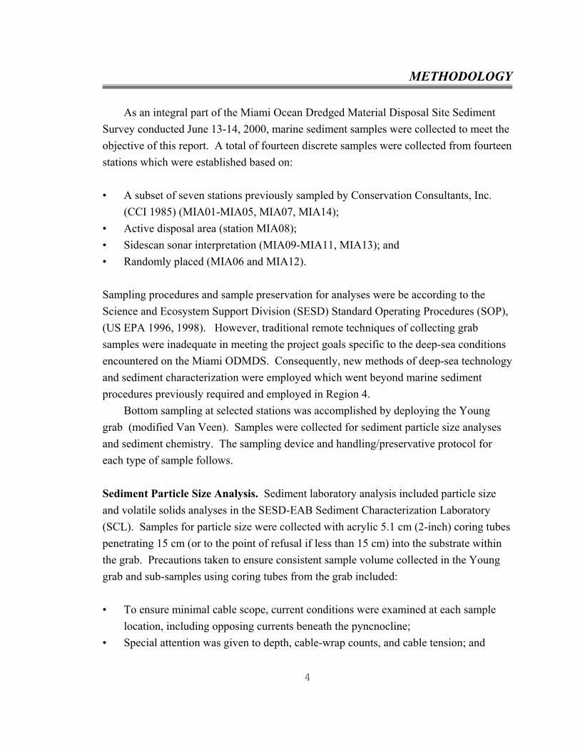
The study area was within and surrounding the Miami, FL ODMDS located offshore Virginia Key (Figure 1). The ODMDS is approximately 3.4 km2 (1.0 square nautical mile, NM), with stations extending up to 5.6 km (3 NM) to each cardinal point of the compass.

A total of fourteen discrete samples were collected from fourteen stations which were established based on:

• A subset of seven stations previously sampled by Conservation Consultants, Inc. (CCI 1985) (MIA01-MIA05, MIA07, MIA14 );

• Active disposal area (station MIA08); • Sidescan sonar interpretation (MIA09-MIA11, MIA13); and • Randomly placed (MIA06 and MIA12).

Bottom sampling at each station was accomplished by deploying a Young grab (modified Van Veen). Samples were collected for sediment particle size analyses and sediment chemistry. Both wet sieve and laser particle size analyses were conducted on sediment samples. Based on assumptions of normality, appropriate statistical analyses were employed to compare data between sample stations and against the previous site survey (CCI 1985). Significance was tested at a 95% confidence level (α = 0.05).

Based on the on-site sediment characterization and sediment particle size analyses (wet sieve and laser), dredged material can be distinguished from the native marine sediments at the Miami ODMDS as follows:

vii

• On-site sediment characterization: In general, stations MIA01 and MIA02 exhibited characteristic native, tropical marine sediments including near white color (5Y 6/2, Munsell Value 6), fine sandy clay loam texture, no strata, no odor, no shell fragments, and benthic organisms (polychaetes). In contrast, marine sediment collected from Stations MIA03 and MIA08 through MIA13 were characteristically stratified, and were slightly darkened with organic matter or minerals not normally associated with tropical marine sediments (i.e., calcites);

• Based on wet sieve particle size analysis alone: Variation in percent particle size classes (inorganic and volatile solids fractions) was observed between Stations MIA01, MIA02, MIA06, MIA07, and MIA14 as compared to Stations MIA03 to MIA05 and MIA08 to MIA13;

• Particle size analysis (laser): By inspection of percent particle size class distribution and percent cumulative finer distribution, Stations MIA01, MIA02, MIA06, MIA07, and MIA14 exhibited finer-grained marine sediment. In addition based on evenness of distribution (skewness and kurtosis), Stations MIA04 and MIA05 were relatively more evenly distributed as compared to other stations; and

• EPA versus CCI (wet sieve): Seven of the fourteen sites (MIA01-MIA05, MIA07, and MIA14) sampled during this EPA study overlapped with the stations sampled in 1985 by CCI. By inspection of the differential distribution of particle size classes, EPA sediment samples were coarser grained as compared to CCI sediment samples. In addition, as evidenced by the cumulative percent distribution curves, this shift was especially pronounced in samples collected from Stations MIA03, MIA04, and MIA05.

viii

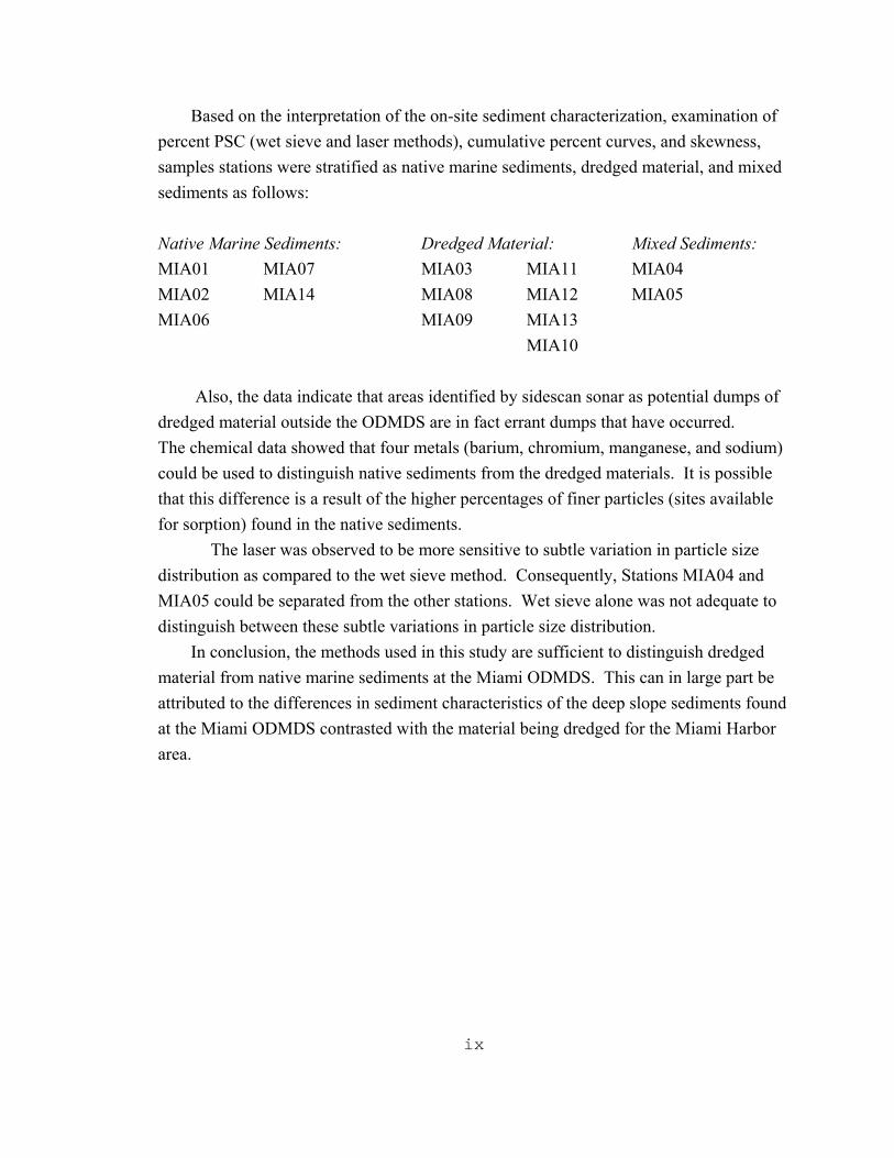
Based on the interpretation of the on-site sediment characterization, examination of percent PSC (wet sieve and laser methods), cumulative percent curves, and skewness, samples stations were stratified as native marine sediments, dredged material, and mixed sediments as follows:

Native Marine Sediments: Dredged Material: Mixed Sediments: MIA01 MIA07 MIA03 MIA11 MIA04 MIA02 MIA14 MIA08 MIA12 MIA05 MIA06 MIA09 MIA13

MIA10

Also, the data indicate that areas identified by sidescan sonar as potential dumps of dredged material outside the ODMDS are in fact errant dumps that have occurred. The chemical data showed that four metals (barium, chromium, manganese, and sodium) could be used to distinguish native sediments from the dredged materials. It is possible that this difference is a result of the higher percentages of finer particles (sites available for sorption) found in the native sediments.

The laser was observed to be more sensitive to subtle variation in particle size distribution as compared to the wet sieve method. Consequently, Stations MIA04 and MIA05 could be separated from the other stations. Wet sieve alone was not adequate to distinguish between these subtle variations in particle size distribution.

In conclusion, the methods used in this study are sufficient to distinguish dredged material from native marine sediments at the Miami ODMDS. This can in large part be attributed to the differences in sediment characteristics of the deep slope sediments found at the Miami ODMDS contrasted with the material being dredged for the Miami Harbor area.

ix

INTRODUCTION

Statement of the Problem. Ocean disposal of dredged materials can affect the environment of a disposal site by disturbing the benthic community and potentially causing long-term reduction of oxygen in the pore waters of the sediments and the overlying waters. Natural oceanographic processes can also be responsible for transporting disposed materials offsite into nearby habitats.

Once a site is chosen for ocean disposal of dredged material, the U.S. Environmental Protection Agency, in cooperation with the U.S. Army Corps of Engineers, is responsible for the management and monitoring of the site. A critical component of Region 4's monitoring program is the characterization and tracking of sediments in and around each Ocean Dredged Material Disposal Site (ODMDS).

Traditional techniques have employed the use of gamma radiation and x-ray fluorescence analyses to discriminate between native and dredged material. However, the Miami ODMDS presents a unique problem in discriminatory analysis given the extreme depths are beyond the physical capabilities of traditional techniques commonly utilized. Consequently, alternate techniques were explored during this study. Results and conclusions derived from this effort will have utility in future monitoring of deeper ocean dredged material disposal activities within Region 4 (e.g., Port Everglades and Palm Beach) and other deep ocean monitoring efforts elsewhere.

Background. The Miami ODMDS was designated in 1995 and a site characterization study was conducted in 1985. Since then over 2.3 million m3 (3 million cubic yards) of dredged material has been disposed at the site. Over 459,000 m3 (600,000 cubic yards) of this material was from an uncharacterized portion of the Miami Harbor West Turning Basin. This material was uncharacterized due to a permitting error. In 1998 a sidescan survey of the ODMDS was conducted to identify the footprint of the disposal mound to aid in future benthic sampling. Several apparent disposal mounds were identified outside of the site boundaries in addition to those identified within the site.

Survey Justification and Rationale. The purpose of this survey was to determine what changes may have occurred to the sediment chemistry and grain size distributions at the disposal site as a consequence of the disposal activity. Sampling station selection were based on previous surveys as well as sidescan data indicating the possibility that some material may have been dumped outside the ODMDS.

2

Objectives. The goal of the study was to manage and monitor the Miami ODMDS in the most environmentally protective manner. The objectives of the study were three-fold (see Table 1 for Data Quality Objectives): 1) characterize selected representative areas of the sea floor from a sedimentological and chemical perspective; 2) explore new methods of sediment collection and characterization where deep sea technology is required; and 3) compare the results of this study against a previous site survey (Conservation Consultant, Inc in 1985). The results and conclusions of this study will be utilized as guidance for future site management, to develop and refine new methods of deep sea sediment exploration, and to “ground-truth” sidescan sonar records from the 1998 survey. Additional uses of the results will be to determine if there is a need for a biological impact study and if disposal of the uncharacterized material caused any adverse environmental impact (such as would be indicated by elevated chemical values).

Survey Location and Description. The study area is within and surrounding the Miami, FL ODMDS located offshore Virginia Key (Figure 1). The ODMDS is approximately 3.4 km2 (1.0 square nautical mile, NM), with stations extending up to 5.6 km (3 NM) to each cardinal point of the compass. Seven stations were selected to coincide with stations sampled by Conservation Consultant, Inc in 1986. One station was positioned in the center of the active disposal area (northwest corner of the ODMDS), whereas four stations were positioned into areas identified by sidescan sonar as possible offsite dumps. The other two stations were a result of improper trans-positioning of coordinates from the survey plan into the navigation system, and were maintained as additional data. The ODMDS boundary coordinates are:

25o45.50'N 80o03.90'W 25o45.50'N 79o02.83'W 26o44.50'N 79o02.83'W 26o44.50'N 80o03.90'W

Hypothesis/ Statistical Tests. The particle size distributions (PSD) of each station and specific size classes across stations were tested for normality using normal probability plots. For normally distributed data, statistical significance was tested using t-tests for dependent samples at a level of significance p < 0.05 (parametric). For data sets that were not normally distributed, chi square analysis was used at a level of significance of p < 0.05 (non-parametric). Testable hypotheses were formulated as:

3

Hypothesis Set 1: Ho = There is no significant difference between physical and chemical analyses of native marine sediments (reference) versus dredged material

H1 = There is a significant difference between physical and chemical analyses of native marine sediments (reference) versus dredged material

Hypothesis Set 2: Ho = There is no significant difference between historic (CCI) and present (EPA) particle size analysis of native marine sediments (reference) versus dredged material

H2 = There is a significant difference between historic (CCI) and present (EPA) particle size analysis of native marine sediments (reference) versus dredged material

Initially, sample stations representative of native marine stations and dredged material were identified by interpretation of previous sidescan sonar records, location with respect to the designated, active disposal area, and disposal records.

METHODOLOGY

As an integral part of the Miami Ocean Dredged Material Disposal Site Sediment Survey conducted June 13-14, 2000, marine sediment samples were collected to meet the objective of this report. A total of fourteen discrete samples were collected from fourteen stations which were established based on:

• A subset of seven stations previously sampled by Conservation Consultants, Inc. (CCI 1985) (MIA01-MIA05, MIA07, MIA14);

• Active disposal area (station MIA08); • Sidescan sonar interpretation (MIA09-MIA11, MIA13); and • Randomly placed (MIA06 and MIA12).

Sampling procedures and sample preservation for analyses were be according to the Science and Ecosystem Support Division (SESD) Standard Operating Procedures (SOP), (US EPA 1996, 1998). However, traditional remote techniques of collecting grab samples were inadequate in meeting the project goals specific to the deep-sea conditions encountered on the Miami ODMDS. Consequently, new methods of deep-sea technology and sediment characterization were employed which went beyond marine sediment procedures previously required and employed in Region 4.

Bottom sampling at selected stations was accomplished by deploying the Young grab (modified Van Veen). Samples were collected for sediment particle size analyses and sediment chemistry. The sampling device and handling/preservative protocol for each type of sample follows.

Sediment Particle Size Analysis. Sediment laboratory analysis included particle size and volatile solids analyses in the SESD-EAB Sediment Characterization Laboratory (SCL). Samples for particle size were collected with acrylic 5.1 cm (2-inch) coring tubes penetrating 15 cm (or to the point of refusal if less than 15 cm) into the substrate within the grab. Precautions taken to ensure consistent sample volume collected in the Young grab and sub-samples using coring tubes from the grab included:

• To ensure minimal cable scope, current conditions were examined at each sample location, including opposing currents beneath the pyncnocline;

• Special attention was given to depth, cable-wrap counts, and cable tension; and

4

5

• To prevent loss of vertical horizons and contamination of the chemical samples, smaller cores were collected during subsampling within the center of the grab.

With the exception of Station MIA10, consistent sampling volumes among the various stations were obtained at all stations.

After settling, the structure and texture of the sediment were observed and recorded, then the clear water decanted and the sediment core placed in a whirl pack, labeled, and frozen for return to the lab. Two replicate samples were obtained at each station. Particle size analyses were determined using a Coulter™ Laser Particle Size Analyzer (Model LS200) in the Sediment Characterization Laboratory (SCL) of the Ecological Assessment Branch (EAB). Volatile solids analyses were determined on seven particle sizes using a modified Wet Sieve Method (Ecological Assessment Branch, Standard Operating Procedures , EAB 2000 as modified from Biological Field and Laboratory Methods for Measuring the Quality of Surface Waters and Effluents, EPA-670/4-73-001).

Prior to particle size analysis, sediment material for particle size distribution (PSD) utilizing the Coulter™ Laser Particle Size Analyzer (Model LS200) was dispersed by adding a dispersing agent (sodium metaphosphate) and placed on an automated shaker overnight. In contrast, in order to be consistent with methods used in the past, no dispersing agent or shaking was conducted on sediment material prior to wet sieve analysis.

Sediment Chemical Analysis. Sediment chemical analysis included pesticides/PCB scan, extractables, metals scan, and classic nutrients (ammonia, nitrates/nitrites, total kjeldahl nitrogen, and total phosphorus) (Appendix A). At each station, samples for metals, nutrient and extractable organic analysis were collected by using 5.1 cm Teflon coring tubes until sufficient volume was obtained. Volatile organic samples were collected in two pre-cleaned and weighed 40 ml vials with a septum seal at each station, with the addition of a 59.1 ml (2 oz.) container at six stations for quality control. Sample handling of cores was similar to that specified above for particle size. The core samples for metals, nutrients and extractable organic compounds were transferred to a glass pan or teflon lined pan and thoroughly mixed. Aliquots of the sample were placed into two 236.6 ml (8 oz.) glass containers. The sample aliquot for nutrients and metals analysis was preserved by freezing. The sample aliquot for pesticides and extractables were preserved at 4EC. VOC collection was conducted utilizing an adaptation to SW846

6

Method 5035 to limit the loss of volatile organics and reduce the possibility of contamination from site conditions, (i.e. diesel fumes from ship operations). Water vials (40 mls) were pre-weighed and filled in the lab with milli-Q water. Sediment was removed directly from the grab at each station, filling the vials one quarter full of sediment. In the ship board lab, approximately 20 mls of sea water was removed utilizing a pipette, leaving approximately 10 mls of sea water over the undisturbed sediment. The standard method of VOC preservation utilizes sodium bisulfate as a preservative. Sodium bisulfate effervesces when it comes in contact with the calcium carbonate found in all marine sediments in the Southeast. The effervescent action then causes a loss of volatile organics. Therefore, once the 20 mls of sea water were removed, and the samples tagged, the samples were preserved by freezing. Samples were placed on their side in the freezer in a protective container to help prevent breakage from freezing.

Statistical Methods. Several methods were utilized to discriminate between native marine sediments and dredged material including (discussed below): on site sediment characterization, PSC within stations (wet sieve and laser), and EPA data versus CCI data (wet sieve). Ultimately, the results of the on site sediment characterization and the PSD analysis were used to stratify stations for interpretation of chemical analysis. Several discriminatory, statistical tests were used to aid in the interpretation of the above datasets including: skewness, standard deviation, t-tests, and chi-square distribution. Data were tested for normality using the Shapiro-Wilkes Test for Normality. Based on the results, parametric (t-tests) or nonparametric (chi-square distribution) tests were employed as appropriate. Data were tested at the 95 % confidence level (α = 0.05).

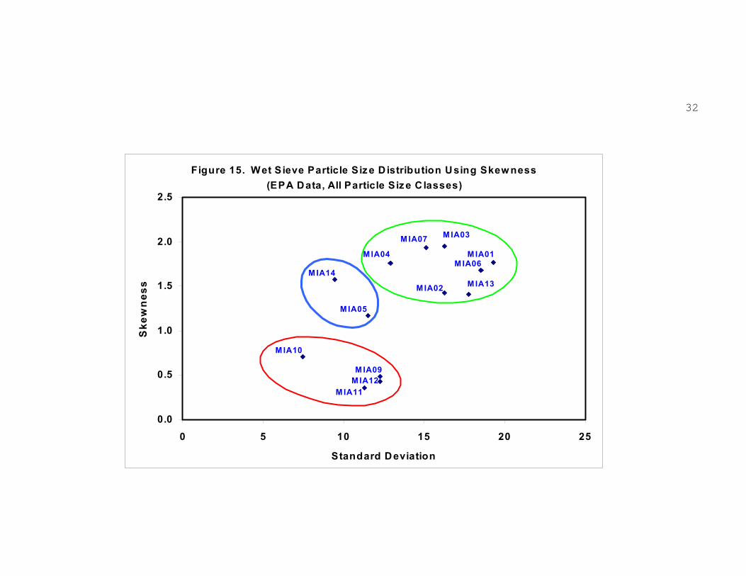
In conjunction with on site sediment characterization, the relative degree of skewness (i.e., variation in PSC) of inorganic fractions plotted against the standard deviation of the means was used, in part, to discriminate between native marine sediment and dredged material. Skewness (third moment in calculus), is a measure of the asymmetry of the PSD in a sediment sample. In general, a frequency curve is skewed with the mode shifted to the right (positive skewness) for an abundance of coarse particles, and to the left (negative skewness) for an abundance of fine particles.

On Site Sediment Characterization. Marine sediments were visually and texturally characterized immediately following collection using a Young box dredge. Sediment

7

characterization included strata, boundary, color (Munsell), texture by feel, and presence or absence of masses, gravel, shell fragments, odor, and benthic organisms.

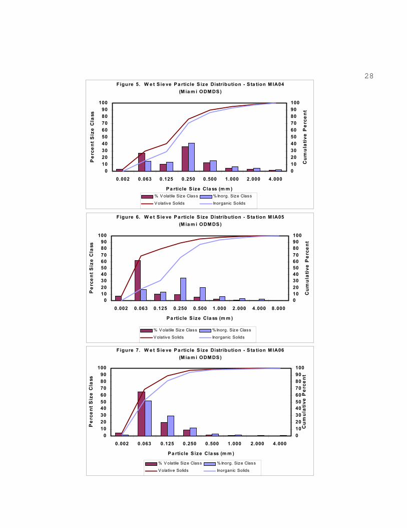
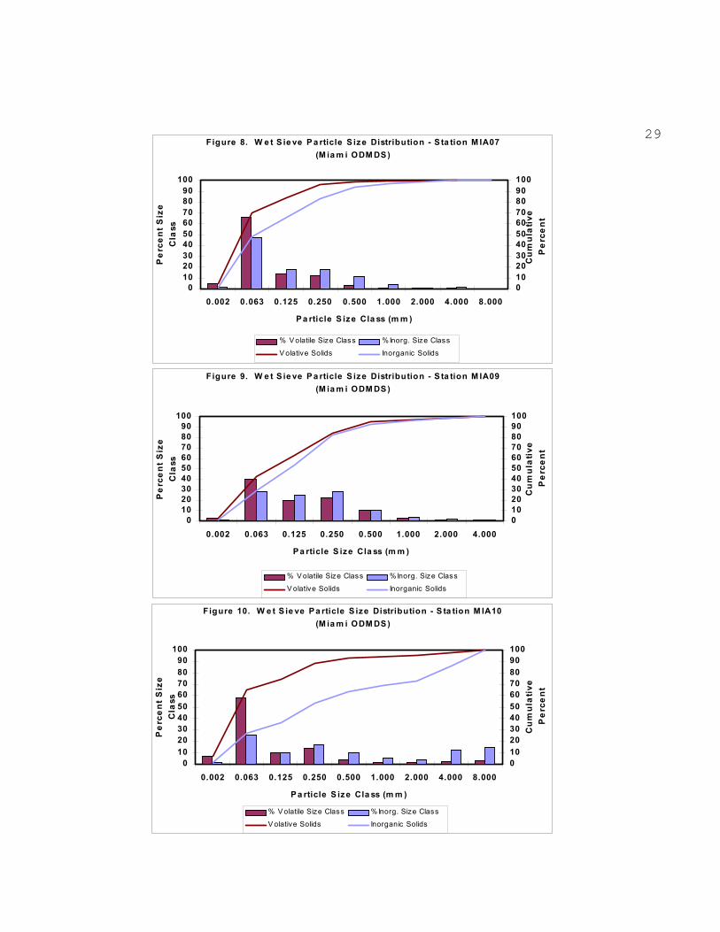
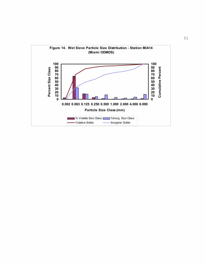
Sediment Particle Size (Wet Sieve). Particle size distributions for both inorganic and volatile solids fractions were plotted on frequency and percent cumulative curves to aid in discriminating between native marine sediments and sediments altered by dredge disposal activities (Figures 2 to 14). Due to an oversight, wet sieve analysis was not conducted on Station MIA08 and is addressed below in Sediment Particle Size (Laser EPA Dataset). Both differential percent (per class) and cumulative percent were plotted against seven particle size classes (PSC, mm): 0.002, 0.063, 0.125, 0.250, 0.500, 1.000, 2.000, 4.000, and 8.000. PSC were arranged on the ordinate axis from left to right (clay fraction to larger than sand fraction, respectively).

CCI (1985) followed, in general, the procedures outlined by Pequegnat et al. (1981) in U.S. Army Waterways Experiment Station Technical Report EL-81-1: Procedural Guide for Designation Surveys of Ocean Dredged Material Disposal Sites. The method consisted of wet sieving the sample through a 62 Fm using a 5 g/l sodium hexametaphosphate dispersant. The sand-shell fraction then underwent grain size analysis by sieving, while pipette analysis was used to quantify the silt-clay fraction. A Tyler Sieve Shaker (Model R-X24) and nested 20.32 cm (8-inch) brass sieves with mesh sizes of 2.0, 1.0, 0.5, 0.25, 0.177, 0.12, and 0.06 mm were used to conduct the sieve analysis. CCI (1985) reported their findings in greater than 2.0, 2.0, 0.50, 0.25, 0.063, and 0.002 mm PSCs. For comparison, the PSC used by EPA were adjusted (mathematically) to match the PSC used by CCI. EPA did not use a dispersing agent prior to wet sieving. Consequently, the assumption was made that the dispersant agent used by CCI did not significantly change the PSD. Three methods of determining relative PSD: skewness, standard deviation, and chi-square distribution.

RESULTS

On-Site Sediment Characterization. In general, Stations MIA01 and MIA02 exhibited characteristic native, tropical marine sediments including near white color (5Y 6/2, Munsell Value 6), fine sandy clay loam texture, no strata, no limestone gravel, no odor, no shell fragments, and benthic organisms (polychaetes) (Table 2). In contrast, marine sediment collected from Stations MIA03, MIA08 through MIA13 were characteristically stratified, and were slightly darkened with organic matter or minerals not normally associated with tropical marine sediments (Tables 2 and 3). Limestone gravel was observed in samples collected from Stations MIA08, MIA10, MIA11, and MIA14. As evidenced by uneven or wavy boundary and masses of different color, stratified samples did not form in place and are interpreted as dredged material.

Sediment Particle Size (Wet Sieve - EPA Dataset). Upon close examination of Figures 2 through 14, variation in percent PSC (inorganic and volatile solids fractions) was observed between Stations MIA01, MIA02, MIA06, MIA07, and MIA14 as compared to Stations MIA03 to MIA05 and MIA09 to MIA13.

Positive skewness was observed in the PSD of samples collected from all stations. However, the degree of skewness varied between stations and was used for discriminatory analysis in the following way. Native marine sediments were characterized by a predominance of fine-grained inorganic and organic material (< 0.125 mm), consequently, exhibited a high positive skewness (skewed right). Based on inspection of PSD (Figures 2 to 14) and skewness (Figure 15), native marine sediments were observed at Stations MIA01, MIA02, MIA06, MIA07, and MIA14. In contrast, marine sediments which were either altered by dredged materials or represented a different native bottom were characterized by the presence of larger particle sizes (> 0.125 mm) and exhibited lower skewness values. These stations included MIA03 through MIA5 and MIA09 through MIA13. This pattern was also observed in the frequency distribution of the volatile solids fractions (Figures 2 to 14).

Building on the interpretation of the on-site sediment characterization, examination of percent PSC (wet sieve method), cumulative percent curves, and skewness, samples stations were stratified as native marine sediments and dredged material initially as follows:

8

9

Native Marine Sediments: Dredged Material: MIA01 MIA03 MIA10 MIA02 MIA04 MIA11 MIA06 MIA05 MIA12 MIA07 MIA09 MIA13 MIA14

Since the dataset was not normally distributed across PSC, a chi-square distribution (non-parametric) was utilized as a confirmation test on the above findings. In this case, stations that were interpreted as native marine sediments (as shown above) were treated as expected PSC and compared against dredged material, observed PSC (Table 4). Stations MIA01, MIA02, MIA06 and MIA07 associated with native marine sediments were found to be significantly different (p < 0.05) from dredged material. Consequently, the results of the chi-square distribution confirmed, in part, the segregation of sample stations shown above.

The objective of the following statistical test was to determine which PSC (among sample stations) changed between native marine sediments and dredged material (shown above). The frequency distribution within specific particle size class was observed to be normally distributed (Appendix B) and the following hypothesis was tested by means of the t-test.

Ho = There is no significant difference between specific particle size classes of native marine sediments (reference) versus the dredged material (wet sieve dataset)

H1 = There is a significant difference between specific particle size classes of native marine sediments (reference) versus the dredged material (wet sieve dataset)

Statistical tests were conducted on specific particle size classes (mm): 0.002, 0.063, 0.125, 0.250, 0.500, 1.000, and 2.000. Significant differences were observed in midrange PSC (mm): 0.063, 0.125, 0.250, and 0.500. No significant difference was observed in PSC (mm): 0.002, 1.000, and 2.000. Thus, significant increases in mid-range PSC were observed at dredged material stations as compared wth native marine sediments. This results complements the relative difference in skewness reported above, in that, marine sediments influenced by dredged material exhibited a more normal PSD due to the introduction of mid-ranged PSC.

10

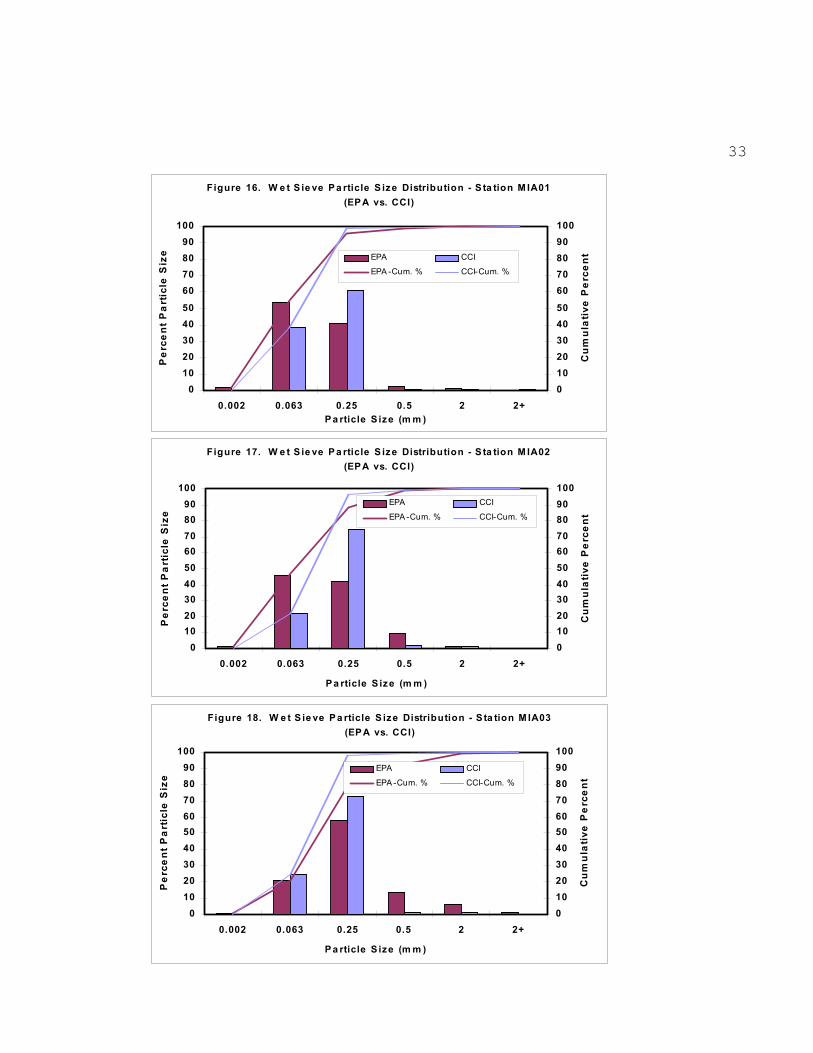
EPA versus CCI. Seven of the fourteen sites (MIA01-MIA05, MIA07, and MIA13) sampled during this EPA study overlapped with the stations sampled in 1985 by Conservation Consultants, Inc. (CCI). As discussed in Methods, CCI reported their findings in greater than 2.0, 2.0, 0.50, 0.25, 0.063, and 0.002 mm PSCs. For comparison, the PSC used by EPA were adjusted (mathematically) to match the PSC used by CCI. EPA did not use a dispersing agent prior to wet sieving. Consequently, the assumption was made that the dispersant agent used by CCI did not significantly change the PSD. Three methods of determining relative PSD: skewness, standard deviation, and chi-square.

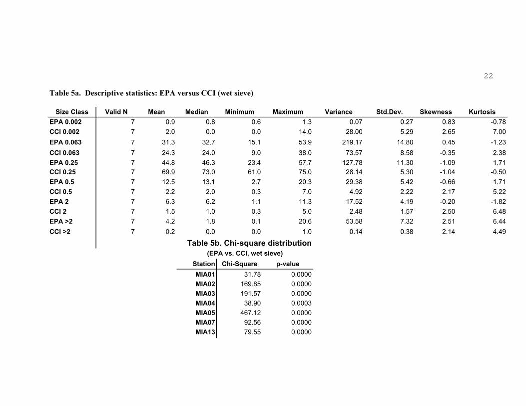
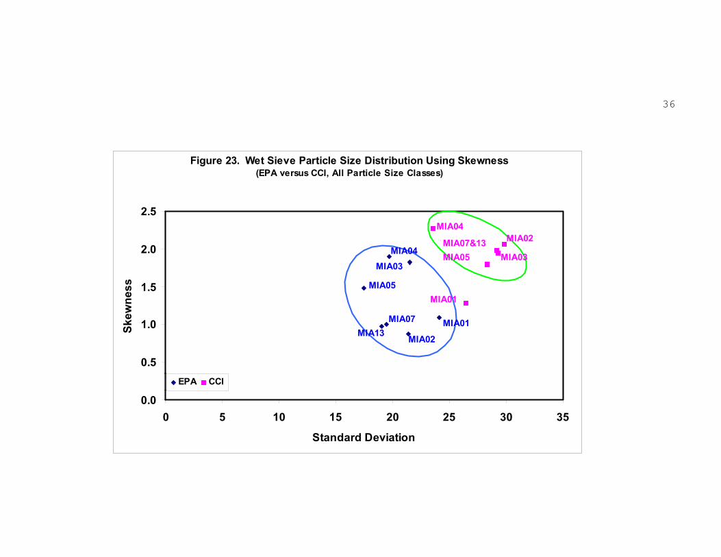
By inspection, EPA sediment samples were shifted down-field (coarser PSC) as compared with CCI sediment samples (Figures 16–22). As evidenced by the cumulative percent distribution curves, this shift was especially pronounced in samples collected from Stations MIA03, MIA04, and MIA05. In order to emphasis this observation, skewness was plotted against standard deviation to determine the degree of separation between the EPA versus the CCI datasets (Figure 23). An excellent segregation of the EPA versus the CCI datasets was observed. Generally, EPA sediment samples were less skewed and had lower standard deviations as compared with CCI sediment samples. Consequently, EPA’s dataset exhibited a more even PSD by the inclusion of coarser PSC with less deviation about the mean PSC as compared with the CCI dataset. As a final confirmation test of the above observations, chi-square distributions were compared between paired sets of data (EPA vs. CCI). Significant difference (p < 0.025) was observed in each of the seven paired datasets (Table 5b).

The above tests were not sensitive to a determination of which PSC was responsible for the difference between the datasets. Hence, the objective of next statistical test was to determine which PSC (between sample stations) were responsible for the significant different observed between the seven paired datasets. Using two-tailed t-tests of each PSC of EPA versus CCI, significant difference (p < 0.025) were observed in PSC 0.250, 0.500, 2.000, and greater than 2.000 mm. By inspection of the arithmetic means of paired PSC, the EPA means were higher than CCI in 0.063, 0.500, 2.000, and greater than 2.000 mm PSC (Table 5a).

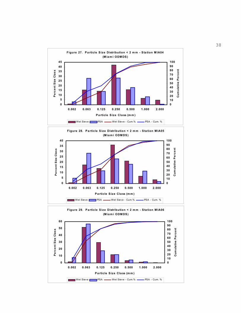
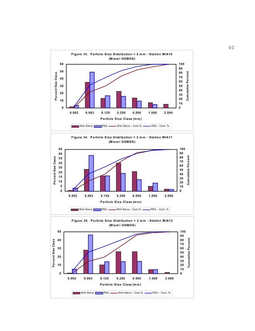
Sediment Particle Size (Laser - EPA Dataset). PSD as determined by laser analyses were plotted on frequency and percent cumulative curves to distinguish between native marine sediments and sediments altered by dredge disposal activities (Figures 24-37). The patterns observed on these graphs show distinctive differences in how the PSC are

11

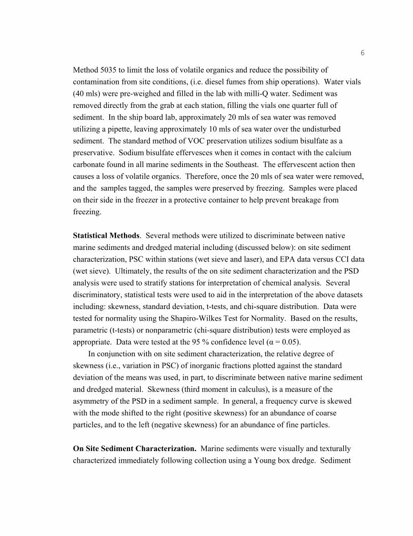
distributed across the various stations related to their proximity to disposal activities as well as their position on the continental slope. Native marine sediments have distributions defined by smaller size fractions with little or no large particles present. This phenomenon is highlighted when D50 values (statistical median) for each station are compared (Figure 38). Stations that were located either within the active disposal area, or thought to have been erroneously dumped on, all have higher D50 values.

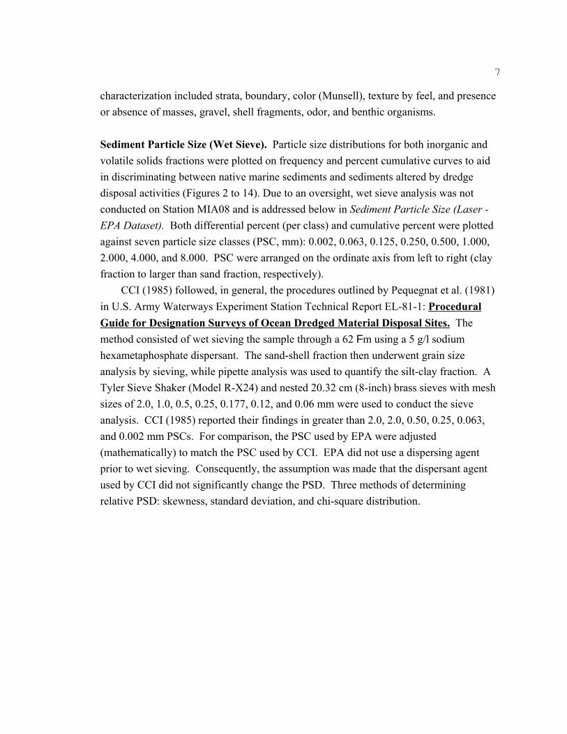
The relative degree of skewness was also plotted against the standard deviation to differentiate between native marine sediment and dredged material (Figure 39). The usefulness and value of comparing skewness and plotting it against the standard deviation has been previously discussed (see above discussion on wet sieve data). The clustering of stations as observed in Figure 39 show how the native marine sediments group together, differently from the other stations. The only anomalies seen are at Stations MIA04 and MIA05. The fact that MIA04 is shallower and closer to the continental shelf (tendency toward sandy sediments) would lead one to expect a less homogeneous PSD. The distribution of MIA05 sediments leads to the conclusion that the sample had a mixture of dredged material and native sediments.

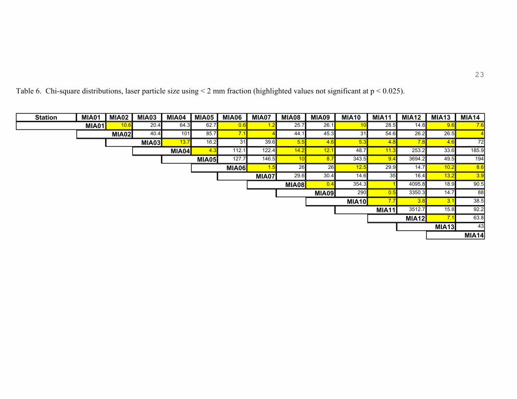
Similar to wet sieve analysis, significant difference between stations on the laser generated analysis was tested using chi-square distribution (α = 0.05, two-tailed) (Table 6). Significant difference was observed between MIA01, MIA03, MIA04, MIA05, MIA08, MIA09, MIA11, and MIA12. MIA02 was also observed to be significantly different from MIA10 and MIA13. However, no significant difference was observed between MIA01, MIA02, MIA06, MIA07, and MIA14. MIA03 was observed to be significantly different from MIA06, MIA07, and MIA14. However, no significant difference was observed between MIA03 as compared to MIA04 and MIA08 to MIA13. MIA04 and MIA05 were not significantly different from each other but were significantly different from MIA06, MIA07, MIA10, MIA12 to MIA14.

Based on the interpretation of the on-site sediment characterization, examination of percent PSC (wet sieve and laser methods), cumulative percent curves, and skewness, samples stations were stratified as native marine sediments, dredged material, and mixed sediments as follows:

Native Marine Sediments: Dredged Material: Mixed Sediments: MIA01 MIA14 MIA03 MIA11 MIA04 MIA02 MIA08 MIA12 MIA05 MIA06 MIA09 MIA13 MIA07 MIA10

12

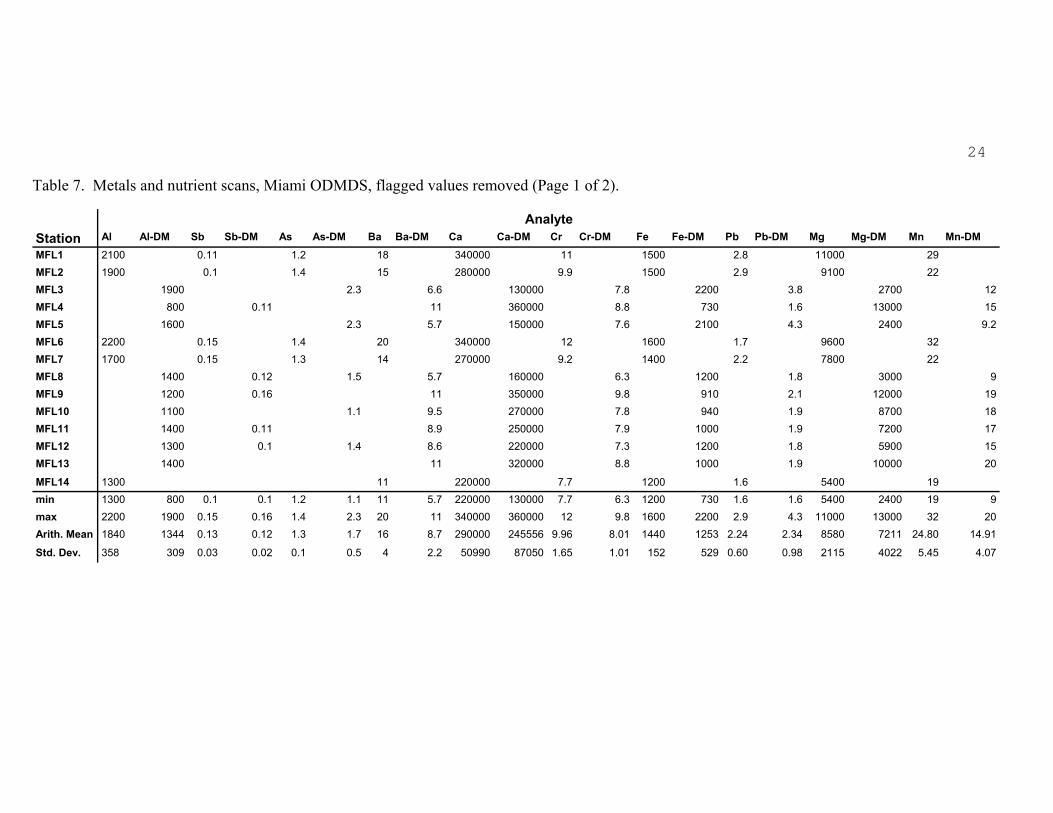
Sediment Chemical Analysis. No pesticides/ PCBs, extractables or nitrates/nitrites were observed above detection limits at the fourteen sample stations. Using a two-tailed t-test, a significant difference (p < 0.025) was observed between native versus dredged material for metals: barium, chromium, manganese, and sodium. By inspection of the means, the four metals were higher in native sediment as compared with dredged material (Table 7 and 8).

The only nutrient that was observed to be significantly different between native as compared with dredged material was total kjeldahl nitrogen (TKN). The mean TKN concentration in native sediments was nearly twice the mean concentration observed in dredged material (1128 versus 670 mg/kg, respectively).

DISCUSSION

In conjunction with on site sediment characterization, the particle size distribution of whole size classes and within specific particle size classes was significantly different between native marine sediments and dredged material.

A major finding of this study was observed by comparing the wet sieve analysis with the laser analysis. Through careful scrutiny of the laser data, two stations (MIA04 and MIA05) were found to be composed of “mixed” sediments. Consequently, the laser method provided better resolution demonstrating its ability to detect more subtle differences in PSD.

The two separate sediment grain size analyses, along with the follow-up statistical analyses, indicates that dredged material can be distinguished from the native marine sediments at the Miami ODMDS. The data also indicates that areas identified by sidescan sonar as potential dumps of dredged material outside the ODMDS are in fact errant dumps that have occurred. However, these types of conclusions should never be made based solely on a single method of analysis. An understanding of the whole environs (e.g., depth, location on the continental shelf vs. continental slope) is also critical to the data synthesis and interpretation for such a study.

The chemical data showed that four metals could be used to distinguish native sediments from the dredged materials. It is possible that this difference is a result of the higher percentages of finer particles (sites available for sorption) found in the native sediments.

The laser was observed to be more sensitive to subtle variation in particle size distribution as compared to the wet sieve method. Consequently, Stations MIA04 and MIA05 could be separated from the other stations. It should be pointed out that one shortfall of the laser analysis is the loss of comparability with the sample’s size fraction above 2 mm. Wet sieve alone was not adequate to distinguish between these subtle variations in particle size distribution. However, depending upon the objectives of future studies, project leaders should use discretion in selecting the method that is best suited for meeting the data quality objectives and anticipated sediment properties encountered during the study.

13

CONCLUSIONS

Sediment samples were collected June 13, 2000 from the Miami Ocean Dredged Material Disposal by the US EPA, Region 4. The objectives of the study were to characterize selected representative areas of the sea floor from a sedimentological and chemical perspective, explore new methods of sediment collection and characterization where deep sea technology is required, and compare the results of this study against a previous site survey (Conservation Consultant, Inc in 1985). We hypothesized there was a significance difference between: 1) physical and chemical analyses of native marine sediments (reference) versus dredged material; and 2) historic (CCI) and current (EPA) particle size analysis of native marine sediments (reference) versus dredged material.

Based on the interpretation of the on-site sediment characterization, statistical analysis of percent particle size classes and cumulative percent curves (wet sieve and laser methods), samples stations were stratified as native marine sediments, dredged material, and mixed sediments as follows:

Native Marine Sediments: Dredged Material: Mixed Sediments: MIA01 MIA14 MIA03 MIA11 MIA04 MIA02 MIA08 MIA12 MIA05 MIA06 MIA09 MIA13 MIA07 MIA10

A careful examination of the sediment regimes that are associated with native marine sediments (Stations MIA01, MIA02, MIA06, MIA07, and MIA14) shows those areas to be located along a similar depth profile on the continental slope. The physical characteristics of different sediment grain sizes means that each would be expected to have different erosional traits and settling rates. Areas such as the five stations listed above which are under similar physical processes, and outside the influence of different sources of material such as dredged material disposal, would be expected to show similar grain size distributions. This explains why these stations, while located far apart, exhibit the same distribution patterns seen in this study.

Seven of the fourteen sites (MIA01-MIA05, MIA07, and MIA13) sampled during this EPA study overlapped with the stations sampled in 1985 by CCI. By inspection of the differential distribution of particle size classes, EPA sediment samples were coarser grained as compared to CCI sediment samples. In addition, as evidenced by the cumulative percent distribution curves, this shift was especially pronounced in samples

14

15

collected from Stations MIA03, MIA04, and MIA05. Using a chi-square distribution, EPA sediment samples at the seven common stations were significantly different from the CCI sediment samples.

We found the Young grab useful in sampling the deep sea stations of this study. However, the following cautionary measures are recommended when attempting to duplicate:

• Carefully exam the current conditions that exist at each location, including opposing currents beneath the pyncnocline, to ensure that minimal scope on the cable exists. If too much scope (angle on the cable) exists upon impact, the device will not ‘grab’ sufficient amounts of material and may not close properly. This type of occurrence will result in lost sediments on the retrieve or inadequate amounts of material, necessitating redeployment;

• Unless the device has a bottom pinger to warn of impending impact, careful attention to present depth, present cable-wrap counts, and tension on the cable are essential. Should you allow the device to sit on the bottom for any extended period of time, vessel movement may tip over the device and waste the time it took for that deployment. Additionally, stopping the cable from paying out any extra length beyond impact could result in cable weight tipping over the device or fouling; again, time wasted on deployment; and

• Special care is needed when subsampling the grab with smaller cores to prevent loss of vertical horizons and contamination of the chemical samples.

Because sampling in depths such as those at the Miami ODMDS requires significant amounts of time due to cable pay-out and retrieval, it is essential that each deployment not be wasted. Following the above recommendations can reduce the amount of ship time necessary to complete such a study.

In conclusion, the methods used in this study are sufficient to distinguish dredged material from native marine sediments at the Miami ODMDS. This can in large part be attributed to the differences in sediment characteristics of the deep slope sediments found

16

at the Miami ODMDS contrasted with the material being dredged for the Miami Harbor area.

REFERENCES

CCI.1985. Environmental Survey in the Vicinity of An Ocean Dredged Material Disposal Site, Miami Harbor, Florida. Report to EPA by Conservation Consultants, Inc. December, 1985. 55 pgs.

USEPA. 1996. Environmental Investigations Standard Operating Procedures and Quality Assurance Manual. US Environmental Protection Agency, Region 4. Athens, GA.

USEPA. 1998. Draft Standard Operation Procedures Ecological Assessment Branch. US Environmental Protection Agency, Region 4. Athens, GA.

USEPA. 1973. Biological Field and Laboratory Methods for Measuring the Quality of Surface Waters and Effluents. EPA-670 / 4-73-001.

17

18

Table 1. Data quality objectives.

DQO Step DQO Description Remarks

Statement of Disposal of dredged materials can adversely Problem affect ocean benthic communities

Decision Management decision on future disposal practices at the site

Objective Characterize selected representative areas of the seafloor from a sedimentological and chemical perspective

Testable Null: No significant difference native marine Alternative: significant Hypothesis 1 sediments (reference) and dredged material difference between

(physical and chemical analysis) reference and disposal site

Testable Null: No significant difference between Alternative: significant Hypothesis 2 historic (CCI) and present (EPA) particle difference between

size analysis of native marine sediments historic and present (reference) versus the dredged material PSD

Statistical Descriptive, Normality, skewness, Chi-Tests Square, t-test of means

Acceptable α = 0.05 MDL: Error and Wet Sieve = 2 µm Limits Laser = 0.375 µm

Sample Size Variance about the mean

19

Table 2: On-site, visual and textural sediment characterization: Miami, Florida ocean dredged material disposal site (Page 1 of 2).

STA LAT/LONG WATER STRATA MUNSELL TEXTURE REMARKS DEPTH COLOR

(ft)

MIA01 25o47.079' / 605 None 5Y 6/2 Fine Sandy Clay No Strata; Few masses (5/10B); No limestone gravel; No 80o03.383' Loam shell fragments; No odor

MIA02 25o46.117' / 80o03.432'

570 None 5Y 6/2 Fine Sandy Clay Loam

No Strata; Few masses (5/10B); No limestone gravel; No shell fragments; No odor

MIA03 25o45.388' / 80o03.360'

566 Surface 5Y 6/2 Fine to Medium Sandy Clay Loam

Infrequent shell fragments; No odor; No limestone gravel

Subsurface 5/10B Fine to Medium Sandy Clay Loam

Common Shell Fragments 1-3mm; No odor; No limestone gravel

MIA04 25o44.999' / 80o04.461'

270 None 5Y 7/1 Fine Sandy Loam No Strata; No limestone gravel; Infrequent small shell fragments; no odor; large polychaete

MIA05 25o45.311' / 80o03.413'

550 Surface 5Y 6-7/1 Fine Sand Thin veneer

Subsurface 5Y 5/1 Silt Loam No distinct boundary; Calcareous clays mixed with numerous shell fragments; No odor; No limestone gravel

MIA06 25o45.00' / 720 None 5Y 6/3 fine Sandy Clay No Strata; Infrequent, small shell fragments <2mm, no 80o02.58' Loam odor; No limestone gravel; plasticity; calcareous sediment;

no benthic

MIA07 25o44.00' / 550 None 5Y 6/1 fine Sandy Clay No Strata; Infrequent, small shell fragments 2-4 mm; few 80o03.367' Loam masses (5/5BG); whole small shells on surface; no odor;

masses 5/5BG No limestone gravel; possibly one polychaete

20

Table 3: On-site, visual and textural sediment characterization: Miami, Florida ocean dredged material disposal site (Page 2 of 2).

STA LAT/LONG WATER STRATA MUNSELL TEXTURE REMARKS DEPTH COLOR

(ft)

MIA08 25o45.337' / 440 Surface 5Y 6/2 Fine to Medium Infrequent shell fragments; No odor; Common small to 80o03.777' Sandy Clay Loam medium limestone gravel

Subsurface 5/10B Fine to Medium Common shell fragments 1-3mm; Some HS- odor on Sandy Clay Loam underside of bluish-green limestone gravel

MIA09 25o45.894' / 80o04.315'

310 none 5Y 6/2 Fine to Medium Sandy Clay Loam

No Strata; No limestone gravel; Infrequent shell fragments; No odor

MIA10 25o45.357' / 80o04.227'

321 None n/a n/a Limestone gravel sized on-site; representative sample returned to EAB Sediment Laboratory

MIA11 25o45.043' / 80o04.009'

373 None 5Y 5/2 Fine-Med. Sandy Clay Loam

No Strata; Common limestone gravel; Infrequent shell fragments; No odor; Frequent polychaetes

MIA12 25o44.467' / 80o03.561'

500 Surface 5Y 6/3 Sandy Loam Stratified; infrequent small shell fragments 1-3 mm; No odor; No limestone gravel

Subsurface 2.5Y 6/1 Silt Loam Frequent shell fragments 1-3mm; No odor; No limestone gravel

MIA13 25o44.396' / 370 None 5Y 6/2 Silt Loam w/ Fine No Strata; Small shell fragments <2mm; No odor; 80o03.976' Sand Plasticity; calcareous sediment; No benthic; No limestone

gravel

MIA14 25o45.070' / 80o03.027'

795 Surface 5Y 6/3 Fine Sand Numerous small shell fragments; No odor; No benthic

Subsurface 5Y 6/1-2 Fine-coarse Larger shell fragments (2-4mm) than surface strata; Sandy Loam Common limestone gravel; Calcareous sand

21

Table 4. Chi-square distribution, wet sieve method using all particle size classes (highlighted values not significant at p < 0.025).

Station 9.1 136.4 155.4 135.1 18.6 44.5 90.8 81.3 83.7 49.3

82.8 96.5 81.1 19.4 20.9 55.9 43.2 44.9 8873 36.4 8.6 12.5 190 76.1 28.8 75.9 1215.6 212.6

2.7 215.3 72.2 24.6 11.8 2990 142.3 215 56.5 23.7 14.4 2966 113.6

17.8 38.5 88.1 75.1 45.1 20.1 50.4 35.3 28.6 4697 38.4

41.9 11.2 28.5 9507 60.4 66.2 127.3 1540 19.7

6.5 4107 66.2 1828 57.9

195.6

MIA01 MIA02 MIA03 MIA04 MIA05 MIA06 MIA07 MIA09 MIA10 MIA11 MIA12 MIA13 MIA14 MIA01 1.1 12228

MIA02 6.2 MIA03 19 29

MIA04 53 28 MIA05 56 4.4

MIA06 82 13419 MIA07

MIA09 MIA10

MIA11 MIA12

MIA13 MIA14

22

Table 5a. Descriptive statistics: EPA versus CCI (wet sieve)

Size Class EPA 0.002 CCI 0.002 EPA 0.063 CCI 0.063 EPA 0.25 CCI 0.25 EPA 0.5 CCI 0.5 EPA 2 CCI 2 EPA >2 CCI >2

Valid N Mean Median Minimum Maximum Variance Std.Dev. Skewness Kurtosis 7 0.9 0.8 0.6 1.3 0.07 0.27 0.83 -0.78 7 2.0 0.0 0.0 14.0 28.00 5.29 2.65 7.00 7 31.3 32.7 15.1 53.9 219.17 14.80 0.45 -1.23 7 24.3 24.0 9.0 38.0 73.57 8.58 -0.35 2.38 7 44.8 46.3 23.4 57.7 127.78 11.30 -1.09 1.71 7 69.9 73.0 61.0 75.0 28.14 5.30 -1.04 -0.50 7 12.5 13.1 2.7 20.3 29.38 5.42 -0.66 1.71 7 2.2 2.0 0.3 7.0 4.92 2.22 2.17 5.22 7 6.3 6.2 1.1 11.3 17.52 4.19 -0.20 -1.82 7 1.5 1.0 0.3 5.0 2.48 1.57 2.50 6.48 7 4.2 1.8 0.1 20.6 53.58 7.32 2.51 6.44 7 0.2 0.0 0.0 1.0 0.14 0.38 2.14 4.49

Table 5b. Chi-square distribution (EPA vs. CCI, wet sieve)

Station MIA01 31.78 0.0000 MIA02 169.85 0.0000 MIA03 191.57 0.0000 MIA04 38.90 0.0003 MIA05 467.12 0.0000 MIA07 92.56 0.0000 MIA13 79.55 0.0000

Chi-Square p-value

23

Table 6. Chi-square distributions, laser particle size using < 2 mm fraction (highlighted values not significant at p < 0.025).

Station MIA02 MIA04 MIA06 MIA08 MIA10 MIA12 MIA14 MIA01 10.6 20.4 64.3 62.7 1.2 25.7 26.1 28.5 14.8 7.6

MIA02 40.4 101 85.7 4 44.1 45.3 54.6 26.2 26.5 4

MIA03 13.7 16.2 39.6 4.6 4.8 4.6

MIA04 4.3 112.1 122.4 14.2 12.1 48.7 11.3 253.2 33.6 185.9

MIA05 127.7 146.5 343.5 3694.2 49.5 194

MIA06 1.5 12.5 29.9 14.7 10.2

MIA07 29.6 30.4 14.6 16.4 13.2

MIA08 0.4 354.3 1 4095.8 18.9 90.5

MIA09 290 0.5 3350.3 14.7

MIA10 7.7 3.1 38.5

MIA11 3512.7 15.8 92.2

MIA12 7.1 63.8

MIA13 43

MIA14

MIA01 MIA03 MIA05 MIA07 MIA09 MIA11 MIA13 0.6 10 9.6 7.1 31 31 5.5 5.3 7.8 72

10 8.7 9.4 26 26 8.6

35 3.9

88 3.8

24

Table 7. Metals and nutrient scans, Miami ODMDS, flagged values removed (Page 1 of 2).

Analyte Station Al Al-DM Sb Sb-DM As As-DM Ba Ba-DM Ca Ca-DM Cr Cr-DM Fe Fe-DM Pb Pb-DM Mg Mg-DM Mn Mn-DM MFL1 2100 0.11 1.2 18 340000 11 1500 2.8 11000 29 MFL2 1900 0.1 1.4 15 280000 9.9 1500 2.9 9100 22 MFL3 1900 2.3 6.6 130000 7.8 2200 3.8 2700 12 MFL4 800 0.11 11 360000 8.8 730 1.6 13000 15 MFL5 1600 2.3 5.7 150000 7.6 2100 4.3 2400 9.2 MFL6 2200 0.15 1.4 20 340000 12 1600 1.7 9600 32 MFL7 1700 0.15 1.3 14 270000 9.2 1400 2.2 7800 22 MFL8 1400 0.12 1.5 5.7 160000 6.3 1200 1.8 3000 9 MFL9 1200 0.16 11 350000 9.8 910 2.1 12000 19 MFL10 1100 1.1 9.5 270000 7.8 940 1.9 8700 18 MFL11 1400 0.11 8.9 250000 7.9 1000 1.9 7200 17 MFL12 1300 0.1 1.4 8.6 220000 7.3 1200 1.8 5900 15 MFL13 1400 11 320000 8.8 1000 1.9 10000 20

MFL14 1300 11 220000 7.7 1200 1.6 5400 19 min 1300 800 0.1 0.1 1.2 1.1 11 5.7 220000 130000 7.7 6.3 1200 730 1.6 1.6 5400 2400 19 9 max 2200 1900 0.15 0.16 1.4 2.3 20 11 340000 360000 12 9.8 1600 2200 2.9 4.3 11000 13000 32 20 Arith. Mean 1840 1344 0.13 0.12 1.3 1.7 16 8.7 290000 245556 9.96 8.01 1440 1253 2.24 2.34 8580 7211 24.80 14.91

Std. Dev. 358 309 0.03 0.02 0.1 0.5 4 2.2 50990 87050 1.65 1.01 152 529 0.60 0.98 2115 4022 5.45 4.07

25

Table 8. Metals and nutrient scans, Miami ODMDS, flagged values removed (Page 2 of 2).

Station Na Na-DM Sr Sr-DM V V-DM Y Y-DM Analyte Zn Zn-DM NH3-N NH3-N-DM TKN TKN-DM TP TP-DM

MFL1 MFL2

12000 11000

4300 3300

5.5 5.4

5.3 4.7

11 13

11 14

1300 1200

340 320

MFL3 MFL4 MFL5

6400 9200 5800

910 4800

910

5

4.7

4.6 4.7

4

11

9.4

5.9 10

530 530 480

470 290 260

MFL6 12000 4100 6.3 5.7 12 9 1200 340 MFL7 9400 3100 4.1 14 12 1100 290 MFL8 5100 890 4.3 4.2 9.1 11 390 390 MFL9 11000 4400 4.8 13 810 290 MFL10 13000 2800 3.9 12 18 960 340 MFL11 8800 2600 4 4.2 8.9 690 340 MFL12 8300 2500 3.9 3.2 6.9 730 200 MFL13 10000 3800 4.6 10 910 280

MFL14 8300 2200 3.8 3.3 11 840 190 min 8300 5100 2200 890 3.8 3.9 3.3 3.2 11 9.1 9 5.9 840 390 190 200 max 12000 13000 4300 4800 6.3 5 5.7 4.8 14 12 14 18 1300 960 340 470 Arith. Mean 10540 8622 3400 2623 5.3 4.4 4.6 4.2 12.5 10.4 11.4 10.5 1128 670 296 318

Std. Dev. 1643 2562 843 1508 1.0 0.5 1.0 0.5 1.3 1.4 1.8 3.8 176 200 63 79

MIA01

MIA02MIA09

MIA10

MIA04

MIA08 MIA03

MIA05MIA11

MIA13 MIA12

MIA07

MIA06

MIA14

MIA01

MIA02 MIA09

MIA10

MIA04

MIA08 MIA03

MIA05 MIA11

MIA13 MIA12

MIA07

MIA06

MIA14

= EPA Stations (June 13, 2000)= EPA Stations (June 13, 2000) = EPA and CCI Stations= EPA and CCI Stations

26

Figure 1. Miami ODMDS station locations.

27

( )

0 10 20 30 40 50 60 70 80 90

( )

0 10 20 30 40 50 60 70 80 90

i l i l

i lids

( )

0 10 20 30 40 50 60 70 80 90

( )

0 10 20 30 40 50 60 70 80 90

i l i l

i lids

( )

0 10 20 30 40 50 60 70 80 90

( )

0 10 20 30 40 50 60 70 80 90

i l i l

i I lids

Figure 2. W e t S ie ve Pa rticle S ize Distribution - S ta tion M IA01 M ia m i ODM DS

100

0.002 0.063 0.125 0.250 0.500 1.000 2.000 4.000

Pa rticle S ize Cla ss m m

Per

cent

Siz

e C

lass

100

Cum

ulat

ive

Per

cent

% V olatile S ze C ass % Inorg. S ze C ass

V olat ve Solids Inorganic So


100

0.002 0.063 0.125 0.250 0.500 1.000 2.000 4.000


Per

cent

Siz

e C

lass

100

Cum

ulat

ive

Per

cent


V olat ve Solids Inorganic So


100

0.002 0.063 0.125 0.250 0.500 1.000 2.000 4.000


Per

cent

Siz

e C

lass

100

Cum

ulat

ive

Per

cent


V olat ve Solids norganic So

28Fi i i i I

( i )

0 10 20 30 40 50 60 70 80 90

( )

0 10 20 30 40 50 60 70 80 90

l i l i l

V ol i li ids

Fi i i i I( i )

0 10 20 30 40 50 60 70 80 90

i l ( )

0 10 20 30 40 50 60 70 80 90

l i l i l

V ol i li ids

Fi i i i I( i )

0 10 20 30 40 50 60 70 80 90

( )

0 10 20 30 40 50 60 70 80 90

l i l i l

V ol i li ids

gure 5. W e t S e ve P a rticle S ize D stribut on - S ta tion M A04 M ia m ODM DS

100

0.002 0.063 0.125 0.250 0.500 1.000 2.000 4.000

P a rticle S ize Cla ss m m

Per

cent

Siz

e C

lass

100

Cum

ulat

ive

Per

cent

% V o atile S ze C ass % Inorg. S ze C ass

at ve So ds Inorganic Sol


100

0.002 0.063 0.125 0.250 0.500 1.000 2.000 4.000 8.000

P a rticle S ze C a ss m m

Per

cent

Siz

e C

lass

100

Cum

ulat

ive

Per

cent




100

0.002 0.063 0.125 0.250 0.500 1.000 2.000 4.000


Per

cent

Siz

e C

lass

100

Cum

ulat

ive

Per

cent



29

)

0 10 20 30 40 50 60 70 80 90

100

( )

0 10 20 30 40 50 60 70 80 90 100

i i l i l

i ids

)

0 10 20 30 40 50 60 70 80 90

100

( )

0 10 20 30 40 50 60 70 80 90 100

i i l i l

i ids

)

0 10 20 30 40 50 60 70 80 90

100

( )

0 10 20 30 40 50 60 70 80 90 100

i i l i l

i ids

Figure 8. W e t S ie ve P a rticle S ize Distribution - S ta tion M IA07 (M ia m i ODM DS

0.002 0.063 0.125 0.250 0.500 1.000 2.000 4.000 8.000


Per

cent

Siz

e C

lass

Cum

ulat

ive

Per

cent

% V olat le S ze C ass % Inorg. S ze C ass

V olat ve Solids Inorganic Sol


0.002 0.063 0.125 0.250 0.500 1.000 2.000 4.000


Per

cent

Siz

e C

lass

Cum

ulat

ive

Per

cent




0.002 0.063 0.125 0.250 0.500 1.000 2.000 4.000 8.000


Per

cent

Siz

e C

lass

Cum

ulat

ive

Per

cent



30

( )

0 10 20 30 40 50 60 70 80 90

100

( )

0 10 20 30 40 50 60 70 80 90 100

l l i l i l

i li

( )

0 10 20 30 40 50 60 70 80 90

100

( )

0 10 20 30 40 50 60 70 80 90 100

l l i l i l

i li

( )

0 10 20 30 40 50 60 70 80 90

100

( )

0 10 20 30 40 50 60 70 80 90 100

l l i l i l

i li


0.002 0.063 0.125 0.250 0.500 1.000 2.000 4.000


Per

cent

Siz

e C

lass

Cum

ulat

ive

Per

cent

% V o ati e S ze C ass % Inorg. S ze C ass

V olat ve Solids Inorganic So ds


0.002 0.063 0.125 0.250 0.500 1.000 2.000 4.000


Per

cent

Siz

e C

lass

Cum

ulat

ive

Per

cent




0.002 0.063 0.125 0.250 0.500 1.000 2.000 4.000


Per

cent

Siz

e C

lass

Cum

ulat

ive

Per

cent



31

(

0 10 20 30 40 50 60 70 80 90

( )

Perc

ent S

ize

Cla

ss

0 10 20 30 40 50 60 70 80 90

Cum

ulat

ive

Perc

ent

i l i ll lids li

Figure 14. Wet Sieve Particle Size Distribution - Station MIA14 Miami ODMDS)

100

0.002 0.063 0.125 0.250 0.500 1.000 2.000 4.000 8.000 Particle Size Class mm

100

% Volatile S ze Cass %Inorg. S ze Cass Vo ative So Inorganic So ds

32

i i i i( )

0 5 10 15 20 25

Figure 15. Wet S eve Part cle Siz e D istr bution Us ng Skew ness EPA Data, All Particle Siz e C lasses

0.0

0.5

1.0

1.5

2.0

2.5

Standard Deviation

Ske

wne

ss

M IA01

M IA02

M IA03

M IA04

M IA05

M IA13 M IA14

M IA07

M IA06

M IA10

M IA11 M IA12 M IA09

33

i icl i i ibuti ion M I(

0 10 20 30 40 50 60 70 80 90

100

2 2+ ( )

0 10 20 30 40 50 60 70 80 90 100

CCI

i icl i i ibuti ion M I(

0 10 20 30 40 50 60 70 80 90

100

2 2+

( )

0 10 20 30 40 50 60 70 80 90 100

CCI

i icl i i ibuti i(

0 10 20 30 40 50 60 70 80 90

100

2 2+

( )

0 10 20 30 40 50 60 70 80 90 100

CCI

Figure 16. W e t S e ve P a rt e S ze D str on - S ta t A01 EPA vs. CCI)

0.002 0.063 0.25 0.5 P a rticle S ize m m

Per

cent

Par

ticle

Siz

e

Cum

ulat

ive

Per

cent

EPA

EPA -Cum. % CCI-Cum. %

Figure 17. W e t S e ve P a rt e S ze D str on - S ta t A02 EPA vs. CCI)

0.002 0.063 0.25 0.5

P a rticle S ize m m

Per

cent

Par

ticle

Siz

e

Cum

ulat

ive

Per

cent

EPA


Figure 18. W e t S e ve P a rt e S ze D str on - S ta t on M IA03 EPA vs. CCI)

0.002 0.063 0.25 0.5


Per

cent

Par

ticle

Siz

e

Cum

ulat

ive

Per

cent

EPA


34

(

0 10 20 30 40 50 60 70 80 90

100

2

( )

0 10 20 30 40 50 60 70 80 90 100

CCI

(

0 10 20 30 40 50 60 70 80 90

100

2 2+

( )

0 10 20 30 40 50 60 70 80 90 100

CCI

-

(

0 10 20

30 40 50 60 70

80 90

100

2 2+

( )

0 10 20

30 40 50 60 70

80 90 100

CCI

-

Figure 19. W e t S ie ve P a rticle S ize Distribution - S ta tion M IA04 EP A vs. CCI)

0.002 0.063 0.25 0.5 2+


Per

cent

Par

ticle

Siz

e

Cum

ulat

ive

Per

cent

EPA


Figure 20. W e t S ie ve P a rticle S ize Distribution - S ta tion M IA05 EP A vs. CCI)

0.002 0.063 0.25 0.5


Per

cent

Par

ticle

Siz

e

Cum

ulat

ive

Per

cent

EPA

EPA Cum. % CCI-Cum. %

Figure 21. P a rticle S ize Distribution - S ta tion M IA07 EP A vs. CCI)

0.002 0.063 0.25 0.5


Per

cent

Par

ticle

Siz

e

Cum

ula

tive

Per

cent

EPA

EPA Cum. % CCI-Cum. %

35

)

0 10 20 30 40 50 60 70 80 90

2 2+ ( )

Perc

ent P

artic

le S

ize

0 10 20 30 40 50 60 70 80 90

Cum

ulat

ive

Perc

ent

-

Figure 22. Particle Size Distribution - Station MIA13 (EPA vs. CCI

100

0.002 0.063 0.25 0.5 Particle Size mm

100

EPA CCI EPA Cum. % CCI-Cum. %

36

i( )

0 5 10 15 20 25 30 35

Skew

ness

CCI

Figure 23. Wet Sieve Particle Size D stribution Using Skewness EPA versus CCI, All Particle Size Classes

0.0

0.5

1.0

1.5

2.0

2.5

Standard Deviation

EPA

MIA01 MIA02

MIA03 MIA04

MIA05

MIA13 MIA07

MIA01

MIA02

MIA03

MIA04

MIA05 MIA07&13

37

( )

0

10

20

30

40

50

60

70

( )

0 10 20 30 40 50 60 70 80 90

i

( )

0

10

20

30

40

50

60

70

( )

0 10 20 30 40 50 60 70 80 90

i

i

( )

0

10

20

30

40

50

60

( )

0 10 20 30 40 50 60 70 80 90

i

i

Figure 24. P a rticle S ize Distribution < 2 m m - S ta tion M IA01 M ia m i ODM DS

0.002 0.063 0.125 0.250 0.500 1.000 2.000


Per

cent

Siz

e C

lass

100

Cum

ulat

ive

Per

cent

Wet S eve PSA Wet Sieve - Cum.% PSA - Cum. %


0.002 0.063 0.125 0.250 0.500 1.000 2.000


Per

cent

Siz

e C

lass

100

Cum

ulat

ve P

erce

nt



0.002 0.063 0.125 0.250 0.500 1.000 2.000


Per

cent

Siz

e C

lass

100

Cum

ulat

ve P

erce

nt


38

icl i i i i i I)

0 5

10 15 20 25 30 35 40 45

icl ( )

0 10 20 30 40 50 60 70 80 90 100

i i

icl i i i i i I)

0

5

10

15 20

25

30

35

40

icl ( )

0 10 20 30 40 50 60 70 80 90 100

i i

icl i i i i i I)

0

10

20

30

40

50

60

icl ( )

0 10 20 30 40 50 60 70 80 90 100

i i

Figure 27. P a rt e S ze D str but on < 2 m m - S ta t on M A04 (M ia m i ODM DS

0.002 0.063 0.125 0.250 0.500 1.000 2.000

P a rt e S ize Cla ss m m

Per

cent

Siz

e C

lass

Cum

ulat

ive

Per

cent

Wet S eve PSA Wet S eve - Cum.% PSA - Cum. %


0.002 0.063 0.125 0.250 0.500 1.000 2.000


Per

cent

Siz

e C

lass

Cum

ulat

ive

Per

cent



0.002 0.063 0.125 0.250 0.500 1.000 2.000


Per

cent

Siz

e C

lass

Cum

ulat

ive

Per

cent


39

)

0

10

20

30

40

50

60

70

( )

0 10 20 30 40 50 60 70 80 90

i

)

0 5

10

15 20 25 30

35 40 45

( )

ila

ss

0 10 20 30 40 50 60 70 80 90

i

)

0

5

10

15

20

25

30

35

40

45

( )

0 10 20 30 40 50

60 70 80 90

Figure 30. P a rticle S ize Distribution < 2 m m - S ta tion M IA07 (M ia m i ODM DS

0.002 0.063 0.125 0.250 0.500 1.000 2.000


Per

cent

Siz

e C

lass

100

Cum

ulat

ive

Per

cent

Wet S eve PSA Wet Sieve - Cum.% PSA Cum. %


0.002 0.063 0.125 0.250 0.500 1.000 2.000


Per

cent

Sze

C

100

Cum

ulat

ive

Per

cent

Wet S eve PSA Wet Sieve - Cum.% PSA Cum. %


0.002 0.063 0.125 0.250 0.500 1.000 2.000


Per

cent

Siz

e C

lass

100

Cum

ulat

ive

Per

cent

PSA PSA Cum. %

40

( )

0

10

20

30

40

50

60

( )

0 10 20 30 40 50 60 70 80 90 100

i

( )

0 5

10 15 20 25 30 35 40 45

( )

0 10 20 30 40 50 60 70 80 90 100

i

( )

0

10

20

30

40

50

( )

0 10 20 30 40 50 60 70 80 90 100

i


0.002 0.063 0.125 0.250 0.500 1.000 2.000


Per

cent

Siz

e C

lass

Cum

ulat

ive

Per

cent



0.002 0.063 0.125 0.250 0.500 1.000 2.000


Per

cent

Siz

e C

lass

Cum

ulat

ive

Per

cent



0.002 0.063 0.125 0.250 0.500 1.000 2.000


Per

cent

Siz

e C

lass

Cum

ulat

ive

Per

cent


41

Fi I( i )

0

10

20

30

40

50

( )

0 10 20 30 40 50 60 70 80 90

i i

i( )

0

10

20

30

40

50

60

70

80

( )

0 10 20 30 40 50 60 70 80 90

i i

gure 36. Pa rticle S ize Distribution < 2 m m - S ta tion M A13 M ia m ODM DS

0.002 0.063 0.125 0.250 0.500 1.000 2.000


Per

cent

Siz

e C

lass

100

Cum

ulat

ive

Per

cent


Figure 37. Pa rticle S ze Distribution < 2 m m - S ta tion M IA14 M ia m i ODM DS

0.002 0.063 0.125 0.250 0.500 1.000 2.000


Per

cent

Siz

e C

lass

100

Cum

ulat

ive

Per

cent


42

)

D50

(mm

)

Figure 38. Particle Size Distribution by D50 - Laser (Miami ODMDS

0.00

0.02

0.04

0.06

0.08

0.10

0.12

0.14

0.16

MIA01 MIA02 MIA03 MIA04 MIA05 MIA06 MIA07 MIA08 MIA09 MIA10 MIA11 MIA12 MIA13 MIA14

Station

Native

Dredge Mat'l

Mixed Sediments

Ske

wne

ss

F igure 39. Laser Particle S iz e D istribution - Particle S iz es < 2 mm

U sing Skew ness 3.0

2.5

2.0

1.5

1.0

0.5

0.0

EPA Stations : 1,2,6,7,14

EPA Stations : 3, 8-13

(no e vide nce o f dre dge m at'l)

(e vide nce of dre dge m at'l)

EPA Stations : 4&5 (e vide nce of dre dge m at'd iffe re nt s e dim e nt type )

l or

0 5 10 15 20 25 30 Standard D eviation

43

sediment survey: ocean dredged material disposal site ... · pdf filesediment survey: ocean...

Documents