sediment movement under combined waves, tide...

Coastal Dynamics 2009 Paper No.67

1

SEDIMENT MOVEMENT UNDER COMBINED WAVES, TIDE AND RIVER DISCHARGE IN A RIVER MOUTH

Xiaojing Niu1, 2, Satoshi Ueyama1, Shinji Sato1, Yoshimitsu Tajima1 and Haijiang Liu1

Abstract Sediment movement around the river mouth is intensive and complicated, owing to the combined effects of short waves, long waves, tide currents and river discharge, which usually leads to great and frequent topography change. This study aims to describe the sediment movement in a river mouth, further to distinguish the contribution of each hydrodynamic component to sediment movement, and to get better understanding on the nonlinear effects to sediment transport and their interactions. A numerical model was developed to simulate the hydrodynamic environment and the movement of color sand tracers. Both field survey and numerical modeling were carried out around the Magome River mouth, which is located on the Enshu Coast, Shizuoka Prefecture, Japan and drains into the Pacific Ocean. Key words: sediment transport, wave-current interaction, color sand tracking, river mouth 1. Introduction Sediment movement around the river mouth is of great importance for estuary environment and of great influence on human being. Sediment accumulation at the river mouth caused by the intensive and complicated sediment movement may greatly reduce the discharge capability of the river and results in serious flood hazard. At some large river mouths, people are suffering from endless dredging to keep enough water depth for shipping. According to some previous investigations (Tajima et al., 2008), sediment movement could cause great topography change in a couple of days under some extreme conditions, such as storm, flood etc. The primary objective of this study is to develop a model that can simulate the sediment movement in such complicated situations.

ShizuokaPrefectureJAPAN

1 km

N

Magome River

Enshu Coast

NakatajimaSand Dune

Ten

ryu

Riv

er

Figure 1. Location of the Magome River

The Magome River mouth studied in this paper is a reconstructed river mouth. In the past, the downstream area of the river often suffered from flood because of the sinuousness and frequent changing of the river mouth. In 1964, a double guide jetty was constructed to fix the river mouth, in order to enhance the discharge capability of the river. It has been proved to be an efficient method to solve the flood problem. However, the problem of shoreline retreat around this area emerged recently and became more and more significant after the construction of several dams along the Tenryu River, which is the main sediment

1 Department of Civil Engineering, The University of Tokyo, 7-3-1 Hongo, Bunkyo-ku, Tokyo 113-8656, Japan.

[email protected] 2 Department of hydraulic Engineering, Tsinghua University, Beijing 100084, China.


2

source for the Enshu Coast. The Tenryu River is located about 4km to the east of the Magome River mouth. The decrease of sediment supply to this area resulted in abrupt shoreline retreat. Especially, the Nakatajima sand dune on the west of the Magome River has been greatly eroded, because the jetty at the Magome River mouth seems to block the westward longshore sediment transport from the Tenryu River mouth. To maintain the sand dune, sand from other place is carried to the Nakatajima sand dune now. However, it’s a time-consuming and high-cost project. If some sediment inside the river mouth could be taken to the Nakatajima sand dune by natural processes, then we might find out a much more feasible and efficient way to maintain the sand dune. Therefore, the investigation on hydrodynamic environment and sediment movement in this river mouth is required.

In most cases, the jetty at the river mouth can intercept the estuary turbidity belt and let tide bring clear water upstream into river mouth. But in case of storm, a large amount of sediment can be brought from offshore into the river mouth basin (Hiramatsu et al., 2008). The hydrodynamic condition in the river mouth is rather complex. Beside tide current and river discharge, there is also a sewage flow draining into the basin. Waves inside the river mouth are also significant, especially when incident wave direction is parallel to the jetty. Topography inside the river mouth might be modified greatly and frequently, due to the complex hydrodynamic environment and the intensive sediment movement.

To capture the feature of sediment movement inside the Magome River mouth, sediment movement is tracked by using different kinds of color sand as tracers, which is a common method adopted in field survey. From field survey we can quantify the color sand content in each sampling point after a certain period and estimate the speed and the amount of sediment movement. However, it’s a rather arduous work to take lots of the samples. By numerical modeling we can look into the detail of sediment movement in any time and any place.

In this paper, a field survey in the Magome River mouth is introduced firstly. Then an associated numerical modeling for the river month is described. Finally, the model is applied to the Magome River mouth, and compared with the observation data of field survey. The results of simulation agree with the results of field survey reasonably, and several observed phenomena are demonstrated by numerical simulation. 2. Field survey Field survey in the Magome River mouth was carried out in 2008. Flow velocities and wave height were measured on Sep13th -14th during the spring tide. Two kinds of color sands were placed inside the river mouth basin in order to trace the sediment movement.

Figure 2. Magome river mouth and the setup of the field survey

2.1. Measurement of the hydrodynamic factors Flow velocities were measured at the three points marked with squares, shown in Figure 2. Velocity meters ‘V1’ and ‘V2’ were electromagnetic flow meters, installed upstream and inside the river basin respectively. Velocity meter ‘V3’ at the right bank of outlet was an acoustic Doppler current meter.


3

Water surface elevations were recorded by wave gauges at the three points marked with triangles, shown in figure 2. Wave gauge ‘H3’ was installed near the left bank at the seaward end of the outlet, wave gauge ‘H2’ was installed near the right bank where the outlet becomes wide, and wave gauge ‘H1’ was installed furthest inside the river mouth. Wave parameters were obtained from the FFT (the Fast Fourier Transform) analysis.

(a) Sep 14th (b) Sep 22th (c) Sep 29th

(d) Oct 13th (e) Nov 8th (f) Dec 12th

Figure 3. Spatial distribution of blue sand

(a) Sep 14th (b) Sep 22th (c) Sep 29th

(d) Oct 13th (e) Nov 8th (f) Dec 12th

Figure 4. Spatial distribution of yellow sand


4

2.2. Tracing the color sand Two kinds of color sand were placed at the blue and yellow points illustrated in Figure 2 during low tide on Sep 13th 2008. The blue sand was placed near the left bank where the sewage drains into river mouth. The yellow sand was placed upstream at the edge of shoal which emerged during the low tide. The amount of injected color sand is about 500kg respectively, and the diameter of color sand is similar to that of local sand, around 0.2mm to 0.4mm. In the following two days, we collected sand samples inside the river mouth hourly. Subsequently, we continued surface sediment sampling during the low tide once in two weeks for three months.

Color sand content in the collected sample was counted by an automated counting machine, which takes sand sample image and recognizes color sand particles by image analysis. Then we obtained the spatial distribution of the color sand after one day, one week, two weeks, one month, two mouths and three mouths, as shown in Figure 3 and Figure 4. The larger mark represents more color sand had been found in the sample. Some blue sand had been found upstream and along the sewage flow. At first only a few yellow sand particles were found in the samples, and after several weeks some had been found scattered in the shoal area. 3. Numerical model A numerical model for the sediment movement in the river mouth has been developed, which includes three associated parts to deal with current, waves and sediment particles movement respectively. These three parts are named as current module, wave module and sediment movement module respectively. Short waves are estimated based on the spectral action balance equation with the effect of current. The nonlinear shallow water equation is then applied to calculate the flow due to tide, river discharge, and long waves. Radiation stress is included to consider the effect from short waves. Following Tajima et al.(2007), the movement of sediment particles is associated with the bottom shear stress under combined waves-current field. 3.1. Current module Based on the shallow water assumption, the governing equations of current are expressed in the Cartesian coordinates as follows.

0p qt x yη∂ ∂ ∂+ + =

∂ ∂ ∂ (1)

2

0bcxx x

p p pq gh M Rt x h y h x

τηρ

∂ ∂ ∂ ∂ + + + + − + = ∂ ∂ ∂ ∂ (2)

2

0bcyy y

q pq q gh M Rt x h y h y

τηρ

∂ ∂ ∂ ∂ + + + + − + = ∂ ∂ ∂ ∂ (3)

where η is the surface elevation; p and q are the flux per unit width in x and y direction; h is the total water depth, h d η= + , here d is the still water depth; g is the gravity acceleration; ρ is the water density. bcxτ and bcyτ are the bottom shear stresses due to mean current component in x and y direction, considering as the summation of the skin friction under combined wave-current field and the form drag due to sand ripples. The skin friction for current is estimated by Madsen’s (1994) boundary layer model. Mx and My represent the diffusion term,

x e ep pM h v v

x x h y y h ∂ ∂ ∂ ∂ = + ∂ ∂ ∂ ∂

(4)

y e eq qM h v v

x x h y y h ∂ ∂ ∂ ∂ = + ∂ ∂ ∂ ∂

(5)

Here, eν is the eddy viscosity. Rx and Ry represent the force due to wave motion, expressed by


5

1 xyxxx

SSR

x yρ∂ ∂

= + ∂ ∂ (6)

1 yx yyy

S SR

x yρ∂ ∂

= + ∂ ∂ (7)

Here, xxS , xyS , yyS are wave radiation stress components, determined by

( )2 11 cos2xxS E n θ = + −

(8)

( )2 11 sin2yyS E n θ = + −

(9)

sin cosxyS En θ θ= (10)

Here, θ is the wave angle; E is the wave energy flux, 218

E gHρ= ; 1 212 sinh 2

khnkh

= +

is the shallowness

parameter. And H is the wave height; k is the magnitude of wave number; h is the water depth. Wave height, wave direction, period can be estimated by the wave module. Governing equations are discretized in a staggered mesh by finite volume method, and the discrete equations are solved by ADI (Alternating Direction Implicit) method. This numerical scheme has been proved efficient and of good stability. 3.2 Wave module A steady spectral action balance equation is applied to model the random waves, which is expressed as follows.

22 2

2

1cos cos2 2

yxb g g

c Nc N c N N NN CC CCx y y y y

θ κε θ θθ σ

∂ ∂ ∂ ∂ ∂ ∂+ + = − + − ∂ ∂ ∂ ∂ ∂ ∂

(11)

where N is the wave action, ( ), , ,N x y f Eθ σ= ; θ is the wave angle. The second term at right side is the diffraction effect proposed by Mase (2001) and Mase et al.(2004). Here, C is the wave phase velocity, Cg is the wave group velocity, κ is a coefficient, 2.5κ = was adopted by Mase (2001) . The characteristic velocities cx, cy and cθ are defined as follows, considering the effect of current.

cosx gc C Uθ= + (12)siny gc C Vθ= + (13)

sin cossinh 2

sin cos cos sin cos sin

h hckh x y

U U V Vx y x y

θσ θ θ

θ θ θ θ θ θ

∂ ∂= − ∂ ∂ ∂ ∂ ∂ ∂

+ − + − ∂ ∂ ∂ ∂

(14)

Here, U and V are the velocity in x and y direction respectively. σ is the intrinsic wave frequency; ω is the absolute frequency relative to a stationary observer, which has a Doppler shift to the intrinsic wave frequency. The dispersion relation of waves with uniform current is expressed as

( )cos sink U Vσ ω θ θ= − + (15) 2 tanhgk khσ = (16)

In equation (11), bε is the coefficient of wave energy dissipation. The energy dissipation can be estimated by Tajima & Madsen’s (2006) model.

( ) ( )2 2exp 1bb g b total b r

total

K NN C E Eh E

ε ξ ξ = − + − ⋅ (17)

where b

brms

HH

ξ = (18)


6

2

2 2

tan5 , tan 025 , tan 0

16

s

s rb

r

K

γ ββ

γ γ

γ β

> −=

≤

(19)

4 tans rγ γ β= + (20) 0.3rγ = (21)

bb

rms

HH

ξ = (22)

( )2

8r

r

g hE

ρ γ= (23)

And the breaking wave height Hb is estimated by 1.5

00 0

1.07 0.59exp 8.6 2.59 tan exp 15.1tanh

b b b b

b b

k H h hk h L L

β = − − + −

(24)

The incident wave is random in terms of both frequency and direction. The incident wave spectrum is generally expressed as the product of frequency spectrum and directional spreading function. The Bretschneider-Mitsuyasu type frequency spectrum and the Mitsuyasu type directional spreading function are used.

Governing equations are discretized by finite difference method. Considering waves are mainly propagating in x direction, x directional derivative is approximated by explicit difference, and y directional derivative and θ directional derivative are approximated by implicit difference. In this way, wave height can be calculated step by step in x direction from offshore to onshore, and in each step wave spectrum is calculated implicitly. This method is economical in memory and effective unless the wave direction depart far from x direction. 3.3 Sediment movement module At first, sediment particles are assumed moving with the same velocity as currents if the local Shields number is larger than the criterion for general movement. Using this assumption, the speed of sediment movement was overestimated comparing with the field observation. Afterward, the model proposed by Tajima et al. (2007) was applied with certain modifications. In their model, the movement of each sediment particle includes two components, a mean movement and a random walk.

,t t ti i s i ix x u t r+∆ = + ∆ + (25)

where t tix +∆ , t

ix are the location of i-th sediment particle at time t and t t+ ∆ ; ,s iu is the mean velocity of sediment movement and ir

is the random walk step for one time step. Tajima’s model followed Madsen’s (1991) bedload sediment transport model and presented the

instantaneous velocity of the moving particles, su , which is determined as a function of bottom shear stress, bτ .

**

max ,0b bs s cr

m b

u uuτ τ

α βρ τ

′ ′ = − ′

(26)

where *cru is the critical bottom shear velocity corresponding to the shear stress just enough to initiate the movement of sand particle on a horizontal plane bed, *mu is the maximum shear velocity under wave-current coexisting field,α (=3.3) is a constant and sβ is a coefficient accounting for the influence of the bottom slope.

( )121 cos 1 tan tan

2s mβ β β φ = + (27)

Here, β is the bottom slope in the flow direction and mφ is the friction angle of moving sand grain. The instantaneous bottom shear stress is expressed as a vector summation of two components due to

mean current and waves.


7

( )2cw

b bc wm wf

u u tτ τ ρ′ ′= + (28)

Here, bcτ ′ is the skin friction shear stress due to mean current, cwf is wave friction factor under wave-current coexisting field. The shear stress bcτ ′ and the friction factors cwf are estimated by Madsen’s (1994) bottom boundary layer model under combined wave-current field. ( )wu t and wmu are the wave orbital velocity vector and its amplitude. To consider the nonlinear effect of nearshore wave, the 2nd order Stokes wave theory was applied to estimate the wave orbital velocity. To consider the dispersion characteristics of sediment movement, a random component based on random walk theory is adopted. Tajima et al. (2007) considered that the sediment took a random walk only in the mean current direction and in the wave-propagation direction, and suggested two different dispersion coefficients for wave and current. In their model, the sediment movement was averaged over one wave period and the time step for calculating sediment movement was larger than several wave periods, so the random walk in one time step was designed to display the orientation effect of wave oscillating motion and mean current. The present model computes the movement of each particle under wave-current coexisting oscillating flow and thus already account for dispersive effects due to wave oscillating motion. Therefore, the random walk in the present model should account for pure dispersive phenomena due to turbulence. Here, the random walk is assumed to occur in arbitrary direction as follows.

0 2 cwr r tε= ∆ (29)

where 0r is the unit vectors in arbitrary direction randomly with each particle at each computational time

step. And the dispersion coefficient, cwε is determined by *cw luε κ= . Here, κ is the Karman’s constant, l is length scale of the near-bottom turbulence which is assumed equal to the boundary layer thickness of combined wave-current field calculated from Madsen’s (1994) model and *u is the bottom shear velocity. 4. Observation and model application 4.1 Hydrodynamic factors The computational domain is shown in Figure 5. The contour shows the topography of the basin. The mesh size is 4m in both x and y direction. At landward boundary, 0mx = , a uniform velocity is used in the whole section, and the measured current velocity at location ‘V1’ is adopted. At seaward boundary,

640mx = , the water level from Omaezaki station, which is located about 45km to east of the Magome River mouth, is adopted as the boundary of current module. The measured wave height and period at the outlet of river mouth are used as the seaward boundary for wave module. The discharge of sewage draining into the basin is considered as a constant value of 1.75m3/s.

x (m)

y (m

)

0 100 200 300 400 500 6000

50

100

150

200

250

0

0.5

1

1.5

2

2.5d (m)

Figure 5. Magome River mouth topography

4.1.1 Tide The calculated water surface elevation at different location is shown in Figure 6(a). Small difference among each location can be found. It’s obvious that the difference during ebb tide is larger than that during flood tide. The difference between the most seaward location ‘H1’ and most landward location ‘H3’ is illustrated in Figure 6(b). The solid line shows the numerical result and the dots show the measured data. The elevation difference of the two meters is estimated as 1.84m, which was added to the measured data. Tendency between the numerical result and the measurement agrees well.


8

0 10 20 30 40 50-1

-0.5

0

0.5

1

t (h)

η (m

)

ηH2

ηH1

ηH3

10 15 20 25 30 35 40

-0.2

-0.1

0

0.1

0.2

t (h)

η H1-η

H3(m

)

calculationmeasurement(ηH1-ηH3+1.84)

(a) Water surface elevation (b) Difference between location ‘H1’ and ‘H3’

Figure 6. Water surface elevation 4.1.2. Current The current in the Magome River mouth contains four components, river discharge, sewage discharge, tide flow and wave induced flow. Figure 7 shows the calculated velocity compared with the measured flow velocity inside the river basin. Seaward flow during ebb tide is stronger than landward flow during flood tide. The simulated results acceptably agree with the measurements.

0 5 10 15 20 25 30 35 40 45-1

-0.5

0

0.5

1

t (h)

U (m

/s)

calculated Ucalculated Vmeasured Vmeasured U

Figure 7. Current velocity inside the river mouth basin

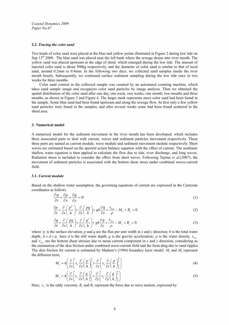
Figure 8 presents the current field at each specified time. Waves induce a circulation in the river basin,

which can be observed when tide current is small, e.g., during low tide and high tide period as illustrated in Figure 8(a) and (c). A simple average of the current velocity is made during one tide period shown in Figure 9. The mean current is mainly contributed by the river discharge and the sewage discharge, and a weak circulation can be found near the sewage outlet.

x (m)

y (m

)

0.6m/s

0 100 200 300 400 500 6000

50

100

150

200

250

x (m)

y (m

)

0.6m/s

0 100 200 300 400 500 6000

50

100

150

200

250

(a) Low tide (t = 10h) (b) Flood tide (t = 14h)

x (m)

y (m

)

0.1m/s

0 100 200 300 400 500 6000

50

100

150

200

250

x (m)

y (m

)

0.6m/s

0 100 200 300 400 500 6000

50

100

150

200

250

(c) High tide (t = 29h) (d) Ebb tide (t = 20h)

Figure 8. Current field at each specified time


9

x (m)

y (m

)

0.2m/s

0 100 200 300 400 500 6000

50

100

150

200

250

Figure 9. Mean current field during one tide period

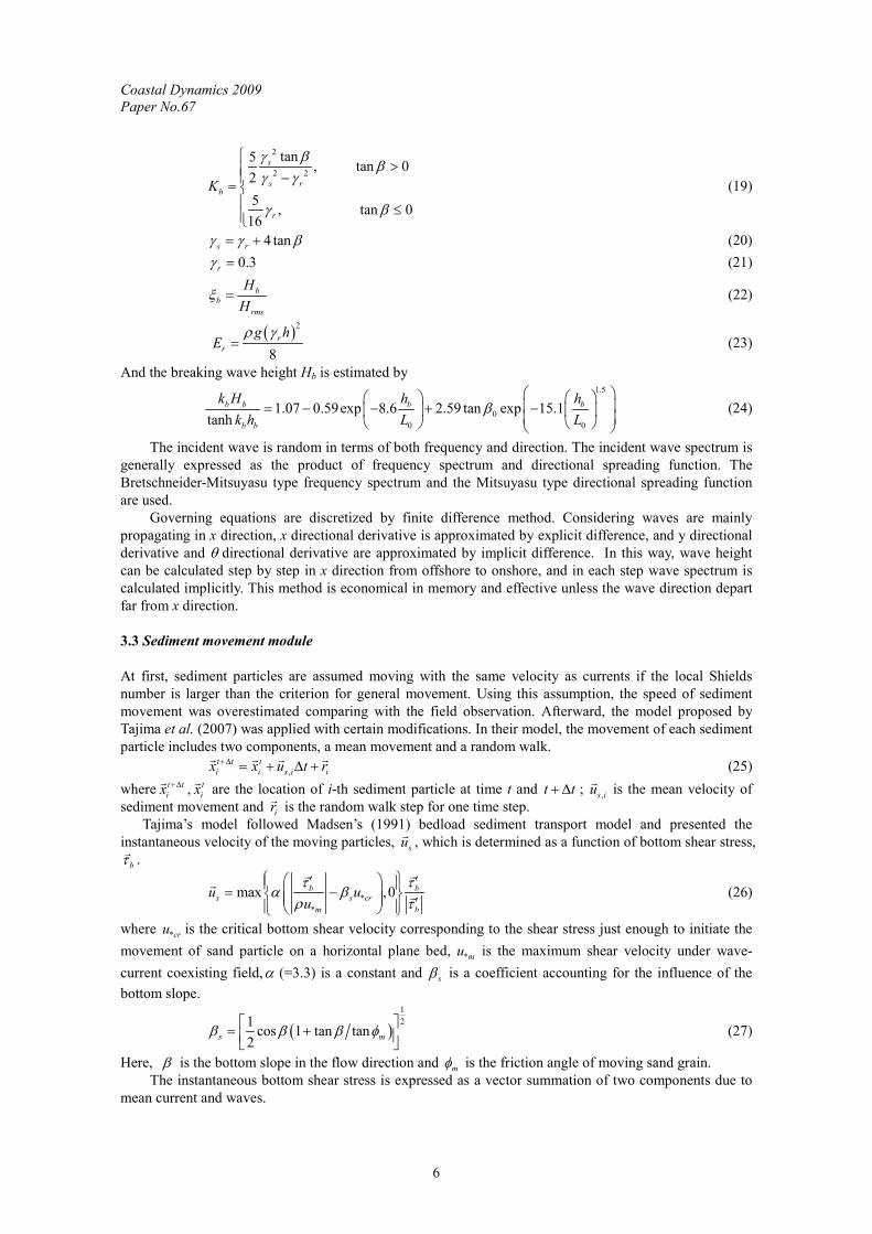
4.1.3. Waves The calculated wave height is compared with the other two measurements inside the river mouth, shown in Figure 10. Points represent the measurement, lines represent calculation results. Computational results agree well with the measurement.

0 5 10 15 20 25 30 35 40 45 500

0.2

0.4

0.6

0.8

t (h)

H (m

)

H1

H2

H3

Figure 10. Wave height at different time

Figure 11 shows the distribution of wave inside the river mouth basin, in which the contour shows the

wave height and the vectors show the direction of wave. Waves are obviously deflected inside the river basin due to refraction and diffraction. Figure 11(a) and (b) show the wave height distribution at the high tide and the low tide respectively. Obviously, waves during high tide invade much further inside of the river basin comparing to that during low tide. It means that waves can reach further upstream which makes the sediment movement inside river mouth more active, while the water depth is larger.

x (m)

y (m

)

0 100 200 300 400 500 6000

50

100

150

200

250

x (m)

y (m

)

0 100 200 300 400 500 6000

50

100

150

200

250

0.1

0.20.30.40.5

H (m)

(a) High tide (b) Low tide

Figure 11. Wave height distribution

Considering that wave period vary due to the effect of current, the intrinsic wave period is calculated by numerical iteration before using the measured wave data as the seaward boundary. It is also found that wave height has periodical alteration even when the wave condition is almost uniform at offshore. That is because waves are affected by the oscillating tidal current in the jetty channel. The present model has the capability to model the interaction between waves and current. The computation results of a wider computational domain show clear periodical variation of wave height in the channel of the river mouth, by


10

using an almost uniform incident wave height, as shown in Figure 12. The dashed line shows the incident wave height and the solid line shows the calculated wave height in the jetty channel. The observation also shows a clear tendency that wave height is amplified by the ebb current. Peaks appear in the measured wave height at the channel around time 20h and 32h without visible peaks of offshore wave height.

0

0.2

0.4

0.6

0.8

1

1.2

0 10 20 30 40 50t (h)

H(m

)

Measured

Offshore data

CalculatedOffshore input

Figure 12. Periodic variation of wave height

4.1.4. Long waves From the field observation, long wave component inside the river mouth basin was found. Long waves can propagate further into the shallow area with less energy dissipation. The mean wave height of long wave components and short wave components is evaluated by spectral analysis. Figure 13 (a) is the result at the most seaward location ‘H3’, and Figure 13 (b) is the result at the most landward location ‘H1’. It shows that the short waves significantly decay inside the river mouth basin, whereas the long waves survive.

Figure 14 shows the transfer function and the phase lag between velocity and water surface elevation. The phase lag of high frequency components is around zero, but the lag of low components is around 0.5π or -0.5π . That characteristic of the low frequency indicates the existence of standing wave, which is the result of interference of the incident wave and the reflected wave due to river bank.

10 15 20 25 30 35 400

0.1

0.2

0.3

0.4

t (h)

H (m

)

10-3

10-2

10-1

0

0.5

1

f (Hz)

Tran

sfer

func

tion

(a) ‘H3’ (a) Transfer function

10 15 20 25 30 35 400

0.1

0.2

0.3

0.4

t (h)

H (m

)

Short waveLong wave

10-3

10-1

10-2

-1

-0.5

0

0.5

1

f (Hz)

phas

e la

g ( π

)

(b) ‘H1’ (b) Phase lag to velocity

Figure 13. The long wave component Figure14. Relation between velocity and water surface

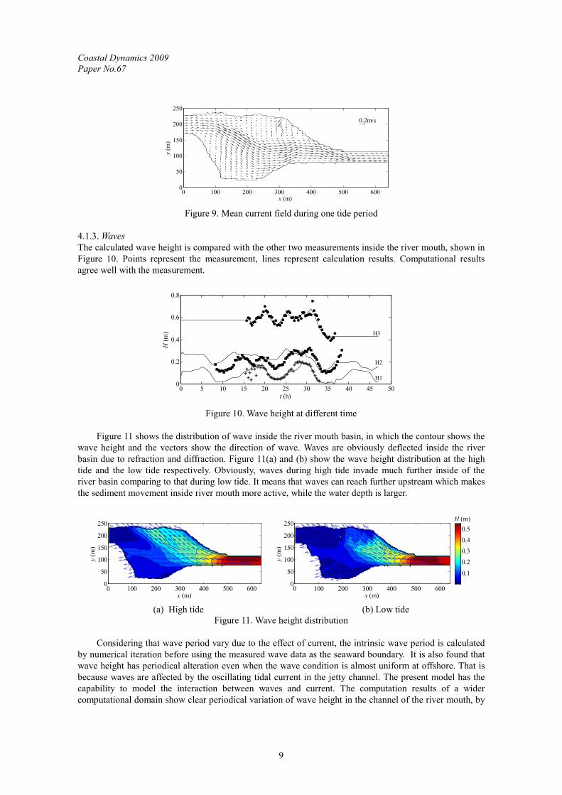
A representative wave with the period of 100s is chosen to study the feature of long wave numerically by shallow water model. A sinusoidal wave with amplitude of 5cm is applied to the seaward boundary. Figure 15 shows the calculated wave height distribution under the condition that initial water level is 0m and current is absent. Standing wave characteristic can be clearly found, and this agrees well with the observation.


11

x (m)

y (m

)

100 200 300 400 500 6000

50

100

150

200

250

0.05

0.1

0.15

0.2

0.25

H (m)

Figure 15. Long wave height distribution

4.2 Sediment movement The color sand movement in the first day of the field measurements was modeled. The number of particles used in the model is 105 for each color sand, which is large enough to capture the feature of sand movement. The critical Shields number adopted is 0.06. In order to represent the mixture of surface sand particles with bed sediments, half of color sand particles is assumed to be moved when the local Shields number exceeds the critical value. Figure 16 shows the spatial distribution of the color sand by tracing large number of particles at each specified time. The yellow dots represent yellow sand particles and the blue dots represent blue sand particles.

The blue particles move landwards during flood tide and seawards during ebb tide mainly along the left bank. Some of blue particles remain at the shoal area after ebb tide, so during low tide there are still some particles found landward to the original location of blue sand, as shown in Figure 16(e) and (i). The sewage flow plays an important role to transport sediment to main flow channel. It is clearly shown in Figure 16 (f) and (k) that some blue sand particles are transported by the sewage flow. The simulated sediment movement agrees well with the observation (Figure 3).

The injection location of the blue particles is near the outlet of sewage flow, as shown in Figure 16(a), where water depth is small. Here waves are relatively intensive, as shown in Figure 11, which offer the main driving force of sediment movement. It is known that wave could induce more intensive bottom shear stress than current, and under the wave condition sediment particles are easy to be picked up. Although the oscillatory wave motion does not induce great net sediment transport, waves still play a very important role in sediment transport under coexisting field of waves and tide current. Under the imaginary situation without waves, the numerical result shows that the blue particles barely move.

In contrast, the original location of yellow sand is further close to the river flow route, as shown in Figure 16(a), where the flow of river and tide is dominant and the effect of waves is weak. At the beginning, the yellow particles are mainly moving along the main flow channel, where the water depth is relatively large. The preceding numerical analysis of hydrodynamic environment in the river mouth shows that along the main flow channel current velocity is large. Consequently sediment particles at main flow channel are dominantly carried by the current and generally tend to move seawards due to the seaward residual current during one tide period. When the yellow particles move into the contraction part of the jetty, where the effect of waves becomes notable, sediment would be transported to the shoal area at the left bank by waves during flood tide and be flushed back to main flow channel during ebb tide, as shown in Figure 16(k) and (l). This is the reason why some yellow particles spread at the shoal. The numerical simulation of yellow sand movement is therefore reasonable with the observation.

The numerical result also shows that sand particles spread in broader area with time. The simulation is performed only for one day, so the distribution of color sand is more concentrated. Generally the color sands will scatter after the longer period as is confirmed in the observed results.

It is noted that some yellow sand is found around its injection location and along the mean flow channel in the field survey, as shown in Figure 4. Because some color sand particles might be covered by the bed sand and remain there until the color sand is exposed again on the surface. It means that some color sand might be found along their tracks. However, in the present model, the topography is assumed to be fixed, and only the mixing percentage is introduced at 50%. Further improvement is required to include topography change and parameter tuning for the mixing layer.


12

x (m)

y (m

)

0 100 200 300 400 500 6000

50

100

150

200

250

x (m)

y (m

)

0 100 200 300 400 500 6000

50

100

150

200

250

(a) t =10h (low tide) (b) t =14h (flood tide)

x (m)

y (m

)

0 100 200 300 400 500 6000

50

100

150

200

250

x (m)y

(m)

0 100 200 300 400 500 6000

50

100

150

200

250

(c) t =17h (high tide) (d) t =20h (ebb tide)

x (m)

y (m

)

0 100 200 300 400 500 6000

50

100

150

200

250

x (m)

y (m

)

0 100 200 300 400 500 6000

50

100

150

200

250

(e) t =23h (low tide) (f) t =26h (flood tide)

x (m)

y (m

)

0 100 200 300 400 500 6000

50

100

150

200

250

x (m)

y (m

)

0 100 200 300 400 500 6000

50

100

150

200

250

(g) t =29h (high tide) (h) t =32h (ebb tide)

x (m)

y (m

)

0 100 200 300 400 500 6000

50

100

150

200

250

x (m)

y (m

)

0 100 200 300 400 500 6000

50

100

150

200

250

(i) t =35h (low tide) (j) t =38h (flood tide)

x (m)

y (m

)

0 100 200 300 400 500 6000

50

100

150

200

250

x (m)

y (m

)

0 100 200 300 400 500 6000

50

100

150

200

250

(k) t =41h (high tide) (l) t =44h (ebb tide)

Figure 16. Spatial distribution of color sand


13

5. Conclusion and discussion Hydrodynamic environment in the Magome River mouth is quite complex owing to the contribution of waves, river discharge and tide, as well as a sewage discharge into the river mouth basin. Field survey inside the Magome River mouth was carried out. Long waves were observed more significantly inside the river mouth in contrast with short waves. Waves invading through the jetty channel were found to be greatly interacted with the tide current.

A numerical model was developed to simulate the complex hydrodynamic environment, including tide current, river discharge, sewage flow, long waves and short waves. Short waves are estimated by the wave energy balance, considering the influence of current. All the other components are simulated by the shallow water equation including the nearshore current induced by shore waves. Reasonable agreement was found between field observation and numerical estimation.

Two kinds of color sand were introduced at two different locations in order to investigate the mechanism of sediment movement. By surface sand sampling in the succedent three month, spatial distributions of color sand inside the river basin were obtained. The sediment movement pattern was evaluated. A numerical model to track the color sand transport was also applied to reveal detailed features of sediment movement in a couple of tide periods. The simulation result reproduced the observed color sand moving characteristics. Acknowledgements This study is a part of Tenryu-Enshu project, “Dynamic sediment management and coastal disaster prevention by advanced technologies”, which is supported by the Special Coordination Funds for promoting Science and Technology of Ministry of Education, Culture, Sports, Science and Technology. References Hiramatsu, H., Tomita, S., Sato, S., Tajima, Y., Aoki, S. and Okabe, T., 2008. Sediment movement mechanism around

the Magome River mouth based on color sand tracer experiments. Annual Journal of Coastal Engineering, JSCE, 55(1):696-700 (in Japanese).

Madsen, O.S., 1991. Mechanics of cohesionless sediment transport in coastal waters. Coastal Sediment 91, 1: 15-27. Madsen, O.S., 1994. Spectral wave-current bottom boundary layer flows. Proceedings of the 24th International

Conference on Coastal Engineering. ASCE, 384-398. Mase, H., 2001. Multidirectional random wave transformation model based on energy balance equation. Coastal

Engineering Journal, 43 (4): 317-337. Mase, H., Yuhi, M., Amamori H., Takayama, T., 2004. Phase averaging wave prediction model with breaking and

diffraction effects in wave-current coexisting field. Annual Journal of Coastal Engineering, JSCE, 51:6-10 (in Japanese).

Tajima, Y., and Madsen, O.S., 2006. Modeling near-shore waves, surface rollers, and undertow velocity profiles. Journal of Waterway, Port, Coastal and Ocean Engineering, 132(6): 429-438.

Tajima, Y., Kozuka, M., Tsuru, M., Ishii, T., Sakagami, T., Momose, K., Mimura, N. and Madsen, O.S., 2007. Tracking sediment particles under wave-current coexisting field. Coastal Sediment 07, 96-109.

Tajima, Y., Liu, H., Sasaki, Y., and Sato, S., 2008. Interactions of morphology change and wave and current fields around a river mouth under severe flood. Annual Journal of Coastal Engineering, JSCE, 55(1):6-10 (in Japanese).

sediment movement under combined waves, tide...

Documents