securitized banking, asymmetric information, and financial ... · securitized banking, asymmetric...
TRANSCRIPT

Securitized Banking, Asymmetric Information, and
Financial Crisis: Regulating Systemic Risk Away∗
Sudipto BhattacharyaLondon School of Economics and CEPR
Georgy ChabakauriLondon School of Economics
Kjell Gustav NyborgISB, University of Zurich and CEPR
February 2012
Abstract
We develop a model of securitized (Originate, then Distribute) lending, in which both publicly
observed aggregate shocks to values of securitized loan portfolios, and later some asymmetrically
observed discernment of varying qualities of subsets thereof, play crucial roles. We find that
originators and potential buyers of such assets may differ in their preferences over their timing of
trades, leading to a reduction in the aggregate surplus accruing from securitization. In addition,
heterogeneity in sellers’ selected timing of trades – arising from differences in their ex ante beliefs
– coupled with initial leverage choices based on pre-shock prices, may lead to financial crises, im-
plying uncoordinated asset liquidations inconsistent with any inter-temporal market equilibrium.
We consider and contrast two mitigating regulatory interventions: leverage restrictions, and ex
ante specified resale price guarantees on securitized asset portfolios. We show that the latter tool
performs strictly better than the former, by ensuring not only bank survival, but also enhanced
social surplus arising from securitized lending in a more coordinated market equilibrium, not
requiring interim leverage buildup to support a “cherry picking” seller trading strategy.
∗We are grateful to Patrick Bolton, Pete Kyle, Frederic Malherbe, the seminar participants at an AXA-FMGconference, the European Finance Association Meetings, the Universities of Zurich, New South Wales, Melbourne,Australian National, Queensland, the Shanghai Advanced Institute of Finance, and the Central Banks of Austriaand Switzerland, for their comments. All errors remain our own.

1. Introduction
Securitization of bank-intermediated loans, via the sales of diversified portfolios backed by these
assets to market-based institutions, which are funded using longer maturity liabilities, has been
a key part of reality in US as well as other developed financial markets for quite a long time.
The presumptive benefits arising from such transactions are due, in addition to the much greater
cross-sectional diversification in the resulting portfolios backing securities, to “inter-temporal
diversification”, owing to which institutions with longer-maturity debt claims, or obligations, are
less vulnerable to any (short-term) aggregate shocks impacting on the current market values of
assets supporting payoffs on these. Hellwig (1998) was one of the first to emphasize such a role for
securitization, in a context of inter-temporal variations in economy-wide interest rates impacting
on interim values of long-maturity loan assets, given fixity of originating banks’ short-maturity
liability claims, and of the returns (interest rates) on their loans.
However, it was only in the previous decade, of “financial innovation”, that we have witnessed
explosive expansion in the securitization of bank-originated lending based on securitization of
credit-backed asset portfolios of a far broader quality spectrum, culminating in an even more
implosive crash leading to a broad-based financial cum economic crisis, considered to be the
worst since the Great Depression of the 1930s. These included credit card debt-based asset
portfolios of varying qualities, and mortgage-backed loan portfolios with much higher debt to
value ratios (also less borrowers’ income information), all subject to potential losses arising from
sectoral shocks with origins beyond economy-wide interest rates. In addition, the financing of
various quasi-independent entities providing funding for such securitization, was often based on
complex “tranching” of the payoffs arising from the asset/loan portfolios which backed up these
liabilities, leading to non-transparency vis-a-vis their default risks.1
In essence, this phase of rapid expansion of securitization - of at least ostensibly lower risk
tranches of portfolios based on bank-originated loans of heterogeneous qualities, and potentially
lower average value than at origination - remained still-born, at or just before the near-closure
(flow-wise) of these markets by 2008. As Adrian and Shin (2009a) have noted, the share of Asset
Based Securities (ABS) held by intermediaries with high and short-maturity leverage ratios -
investment and commercial banks and sponsored investment vehicles - was almost two-third at
the end of 2008, with the remainder held by mutual and pension funds, as well as insurance
companies et al. Earlier in the process, as securitization markets exploded over 2002-2007 (new
issuance sharply slowed over 2007-8, following bad news on some securitized funds), their funding
1When securitized loan portfolios, to be sold by their originating agents to others, do contain payoff defaultrisks which may be mitigated by better ex ante screening and ex post monitoring by their originators, there is anobvious role for some degree of such tranching of their ex post payoffs. For example, originating agents holding onto their lowest priority (equity) tranches, would serve to better incentivize such screening cum monitoring, whiledisposing of their higher priority tranches would enable them to divest other risks connected to the future interimmarket valuations of these assets.
2

by the investing firms was provided largely via increases in their leverage ratios, either directly
as with the investment banks, or within “off the book” special purpose entities sponsored by the
larger commercial banks, quite often in the form of overnight Repurchase contracts, or Repos.
Subsequently, declines in the market valuations of the underlying asset-backed portfolios,
coupled with asymmetric information on their qualities leading to Lemons issues vis-vis mutually
acceptable trade prices, led to Runs in these Repo markets. These in turn led to the possibility
- in some cases reality - of Runs on these investing firms, leading to both higher spreads on
their Repo rates, as well as enhanced “haircuts”, or margins, imposed on such financing. Gorton
and Metrick (2009) have documented these crisis-induced phenomena across securities, as well as
inter-bank, markets. One of their key findings, elaborated on in Gorton and Metrick (2010), was
that post-crisis effects on spreads and haircuts also occurred in securitization markets other than
those backed by sub-prime mortgage backed assets, including on credit-card receivables based
portfolios. On the other hand, the impact on rates and haircuts was much lower for corporate
bonds, which are held largely by investors with either low fixed liabilities, or those of longer
maturities. In particular, yield differentials on industrial bonds of differing categories (AAA vs
BBB) widened in the financial crisis of 2008-9 to a far lesser extent, than those on banks’ ABS
(asset based securities).
These circumstances, and findings, have clearly called for a systematic program of research,
on the functioning and potential vulnerabilities of a “market based banking” system, in which
banks with specialized expertise originate, package, and distribute portfolios of securities to other
financial market participants. In the initial stage of a very rapid expansion of such markets, only
a few firms may have had the required expertise to evaluate risks associated with such portfolios,
to create tranches of these varying in seniority and risk for sale to the ultimate investors, such as
pension funds and insurance firms. During this phase, many securities remained in the portfolios
of these specialized entities, investment banks and the sponsored investment vehicles and conduits
of large commercial banks. This was associated with large increases in their leverage, often of
a short-term nature. The resulting increase in funding for the originated assets was often also
associated with increases in the prices of such assets in the short run – Adrian and Shin (2009b) –
allowing for easy refinancing of loans made to finance these. As a result, medium-run repayment
risks pertinent to affiliated credit-backed portfolios were difficult to judge, as compared to on
corporate bonds, by outside rating agencies as well as by the suppliers of short-term funding to
the initial portfolio owners. But, ultimately, when these asset price “bubbles” proved not to be
sustainable, it led to values of securities based on loans made to finance such assets collapsing,
resulting in attempted deleveraging via liquidations, and further drops in these prices. Shin
(2009) provides a clear outline of such a process of credit expansion and collapse; on pioneering
earlier work on this set of themes, see especially Geanakoplos (2010).
Several recent papers have amplified and elaborated on micro-economic foundations for bank
3

behavior and “systemic risk” - of asset price declines and potential bank failures - in these
settings. Acharya, Shin, Yorulmazer (2010), and Stein (2010), have examined this process further,
by characterizing banks’ ex ante portfolio choices, over risky long-term loans vs risk-free liquid
assets. Liquidity for the purchase of the long-maturity assets of banks, which are sold to service
their debts in low return states, is provided by a combination of other banks which have surplus
liquidity, as well as by outside investors who are less efficient at realizing value from these assets.
Both sets of authors emphasize the externalities on asset prices arising from such inefficient
liquidation, that an individual bank may ignore in making its ex ante portfolio choice. Stein
focuses on the ostensible liquidity premium (cheaper short-term debt) banks may obtain, with
excessive investment in illiquid assets to be sold later at a discount to outside investors in a bad
state of nature. Acharya et al emphasize that an originating bank’s anticipated return on its long-
term assets/loans would not be fully “pledgeable” to facilitate additional interim refinancing, to
stave off such asset sales in adverse states.
In contrast to these papers, in which an originating institution sells its longer-term assets, or
loans, only in low individual or aggregate return states, trying to avert default, Bolton, Santos
and Scheikman (2010) develop and analyze another model in which securitization of originated
assets to markets is an ongoing, and essential, part of the investment process in longer-maturity
and risky assets. The market participants who are potential buyers of these assets ascribe higher
values to them than their originators do, at least contingent on an aggregate value-reducing
shock, which leads their originating institutions to consider selling these assets. Their focus is on
endogenizing the timing of these asset sales, by short-run (SR) funded to long-run (LR) investors,
during a time interval following upon such an aggregate shock. Over that period, originators (or
interim holders) of securitized asset portfolios come to know more about the qualities, in terms of
prospective future payoffs, of subsets within their holdings. Then, if they had not sold all of their
holdings at the start of this stage, the market price would change, to reflect their incentive to sell
only those asset classes on which they have bad news, or at best no idiosyncratic news beyond the
public aggregate shock. Indeed, Bolton et al (hereafter BSS) make a strong assumption, that for
the subset of an SR’s assets on which she has received good news, there is no longer any wedge
between their values as perceived by SR vs LR investors. Hence, given that the LR investors
face an opportunity cost of holding liquidity to buy such assets, there are no gains to be realized
via SR agents trading good assets with LRs.
Building on the last observation, BSS then show that whenever a Delayed trading equilibrium
- in which SRs wait until asymmetric information is (thought to be) prevalent, and then sell only
their “bad” and “no new information” assets to LRs - exists, despite a “lemons discount” in its
equilibrium market price, it Pareto dominates an Early trading equilibrium, for both SR and LR
agents, in an ex ante sense. It is also associated with relatively higher equilibrium origination of
the long-maturity risky asset by SR agents, together with greater outside liquidity provision by
4

LR investors. Therefore, the overall thrust of their conclusions is in sharp contrast with those of
Acharya et al (2010), and Stein (2010). In discussing various policy implications of their model in
a companion paper, BSS (2009), they suggest that when the Delayed trading equilibrium might
not exist – owing to the opportunity cost of holding liquid assets for LR agents, coupled with
prices reflecting asymmetric information about the qualities of assets to be sold therein - a key
role of government policy ought to be that of providing a price subsidy to restore its existence,
complementing the functioning of private purchasers.
Despite the richness of its framework, and the elegance of its analysis, these BSS conclusions
leave many issues unanswered, and raise other questions. There is, for example, no clear “tipping
point” at which a Crisis arises, besides when SR agents discover that there is no delayed trading
equilibrium price at which they are willing to trade medium quality assets, about which they
have no additional news beyond the initial average value-reducing aggregate shock.2 In reality,
significant doubts about the sustainability of high and safe (flow) returns on sub-prime mortgage-
backed securities arose by mid-2007, while the realization of a financial crisis, with sharply
enhanced haircuts and yields related to credit granted based on such assets, did not materialize
until mid-2008. During this long interval, there were also reports of some (investment) banks
divesting, or curtailing purchases of, mortgage-backed securities, so that uniform co-ordination
on a (potential) Delayed Trading equilibrium is far from evident. Rather, it suggests to us
the possibility of developing differences in opinion among SR agents, about the (medium-term)
likelihood of continuation of a benign state for mortgage-backed securities as a whole, leading to
their making differing choices on the timing of trades in these assets, an outcome infeasible in
BSS (2010). Furthermore, the leverage choices made by SR agents who chose not to divest their
risky asset portfolios early, plays no role whatsoever in their model.
For these reasons, concerning our sense that SR agents’ possibly divergent (from 2007 on-
wards) beliefs, regarding the likelihood of an adverse shock to values of sub-prime mortgage-
backed securities as a whole, had an important impact on their choices of timing of trade on
the extant holdings thereof, as well as future investments in these, we develop an alternative
analysis otherwise in the spirit of the BSS framework. In sharp contrast to them, we assume that
the valuation wedge that arises between SR and LR agents, following upon an average value-
reducing aggregate shock, applies to all asset subsets, irrespective of their heterogeneous qualities
as discerned by SRs; Chari et al (2010) assume the same in a reputation-based secondary market
model.3 We examine the potential existence of both delayed and early trading equilibria, as in
2Indeed, in all of the numerical examples of BSS (2010) in which a Delayed Trading equilibrium does exist -and Pareto dominates the Early trading equilibrium - it is only the LR agents who gain strictly, as a result ofincurring lower opportunity costs of providing outside liquidity to SRs. It appears to us to be more than a trifleironic, to base their theory of financial crises on the unanticipated non-existence of the Delayed equilibrium forother parameter values, on the part of SR agents who adopt such a trading strategy despite expecting No strictgains relative to trading earlier. In contrast, in our model SRs gain strictly from delayed trading.
3BSS (2010) assume that such a payoff valuation wedge, across SRs and LRs, disappears for subsets of assetsdiscerned (asymmetrically by SR agents) to be of the highest quality. They base this precept on the assumption
5

BSS (2010), and agents’ preferences over these. We show, in sharp contrast to the BSS conclu-
sions, that LR agents are always worse off in a delayed trading equilibrium whenever it exists, as
compared to in the early trading equilibrium for the same exogenous parameters. SR agents, on
the other hand, may be better off in such a delayed trading equilibrium, but that is the case only
if their ex ante prior, regarding the likelihood of the benign aggregate state continuing - the ad-
verse aggregate shock not occurring - is above an interior threshold level. In essence, sufficiently
“exuberant” ex ante beliefs are essential for the delayed trading equilibrium to be preferred by
(some) SRs. As in BSS (2010), such an SR-preferred delayed trading equilibrium is associated
with (weakly) higher investment in the long-term risky asset, and lower (indeed zero) holding of
inside liquidity by SRs. However, the overall surplus from asset origination and trading, summed
across SRs and LRs, is strictly lower in our delayed, as compared to early, trading equilibrium,
a result yet again in sharp contrast with the conclusions reached by BSS (2009, 2010).
We then consider, again consistent with our view of empirical reality, a scenario in which a
subset of optimistic/exuberant agents, who ascribe a lower likelihood to the adverse aggregate
shock arising, make their choices based on the delayed trading strategy, whereas other SR (as well
as LR) agents, who are less optimistic, make their trades immediately, even before the aggregate
shock has arisen. Such immediate trading plays a key role in our model, unlike in BSS (2010).
We use this scenario to sketch a plausible process for a Financial Crisis, in which some “price
discovery” from immediate trading by a subset of SR and LR agents serves to provide a basis for
Leverage choices of other SR agents, who plan to trade later in a Delayed trading equilibrium,
as outlined above. We then show that even small changes in the beliefs of the less optimistic LR
agents, via its impact on their offered immediate trading prices, may lead to (Repo) Runs by the
short-term creditors of optimistic SRs. The resulting attempted asset sales, by those SR agents
who had planned to trade a proper subset of their assets in a Delayed equilibrium, leads then
to a “market meltdown”, prior to a stage in which idiosyncratic asymmetric information about
subsets of their held assets has accrued to SRs. The market then collapses, and stays that way.
In other words, adverse selection pertinent to delayed trading serves to provide a backdrop for,
rather than the immediate triggering mechanism in, a process of financial crisis. Unanticipated
non-existence of a delayed trading equilibrium plays no role in our model.4
that the aggregate shock to asset payoffs has absolutely no impact on this subset. To us, this assumption seemsmore like a notational simplification, rather than a compelling one. As long as even these subsets are subject tosome likelihood of paying off less than their maximum levels, conditional on an adverse aggregate shock, outsideproviders of leveraged financing to SRs who retain such assets would demand equity injections to ensure the safetyof their debt, as with asset subsets subject to higher likelihoods of low payoffs. That would, in turn, lower theiroverall pledgeable value to investors, as in Diamond and Rajan (2000), owing to greater rent extraction by bank(SR) “insiders”. Further, under asymmetric information mere retention, chosen by them, can not signal quality.
4See also Heider et al (2010) for a model of inter-bank markets, a la Bhattacharya and Gale (1987), which mayfail to function owing to asymmetric information across banks, about the quality of their collateral assets. Hellwig(2008) cautions all modelers, of financial crises in a market based banking system, to take into account not just debtand “excessive maturity transformation”, but also other dimensions of what he terms “market malfunctioning”. Asan example, he refers to risk-assessment, and ensuing leverage choices, by SR agents predicated on observed price
6

Our paper is organized as follows. In Section 2, we provide an overview of the model in
BSS (2010), emphasizing the departure point for our variation on it. Section 3 deals with our
characterization of the manifolds of early and delayed trading equilibria in our setting. Section 4
develops the implications of mis-coordination - across SRs’ trading strategies and leverage choices
- for financial crises. In Section 5 we compare two significant policy interventions: leverage
restrictions, and guaranteed ex ante resale price supports, both of which can mitigate the impact
of such mis-coordination. In Section 6, we conclude, with a discussion of other related recent
literature.
2. The Model
In this Section we present the “originate and distribute” model, inspired by BSS (2009). In
contrast to the model of BSS, where a subset of assets may pay off early, in our model all assets
pay off at the same, but stochastic, terminal date. We further demonstrate that this departure
from BSS has a very significant effect on the structure of equilibrium, which in turn has rich
implications for the understanding of financial crises, which we elaborate on in Sections 4 and 5.
2.1. Outline and motivation for “originate and distribute”
There are four dates, t = 0, . . . , 3, and two classes of institutional agents, with differing investment
opportunity sets and inter-temporal preferences, which are implicitly related to their differing
liability maturity structures. Thus, there are potential gains from trade, as outlined in the
Introduction and discussed below. The timing and extent of such trade, and its equilibrium
implications for initial portfolio choices and welfare, are the foci of our analysis. Agents make
their initial investment choices at t = 0 and may engage in trade at the early and late interim
dates, t = 1, 2. (Later we will consider trading immediately, following upon investment.) All
assets pay off by t = 3, at the latest.
Short-run (SR) agents, funded with short-maturity liabilities, are uniquely capable of orig-
inating long-maturity risky assets, but they ascribe a lower valuation to holding such assets to
maturity, especially if the economy is “shocked”,5 than the other set of agents in the model, Long-
run (LR) investors. One can think of SR agents as representing banks that are funded largely
with short-term liabilities. LR agents can be thought of as pension, insurance other investment
funds that have to cope with longer-duration liabilities, and hence are less concerned with the
interim fluctuations in the values of risky long-term assets. As a result, there are potential gains
volatility prior to any adverse aggregate shock. Our notion of ex ante leverage choices based on offered - but nottaken, by optimistic SR agents - immediate trading prices, is based on the same notion, but amplifies it via linkingit to inter-temporal trading strategy choice. That serves to resolve Hellwig’s justified bafflement, regarding theextent of price declines on higher tranches of asset based securities, which defied any reasonable payoff projections.
5In the sense of an economy-wide, non-diversifiable, negative payoff shock to securitized assets.
7

from trade to be had from SRs selling risky assets that they originate on to LRs at one of the
interim dates.
However, LRs face opportunity costs associated with holding liquidity, to enable them to buy
SR-originated assets. This arises in the form of an alternative long-term investment that pays
off at t = 3. These alternative investments have diminishing marginal returns, implying that
LRs face increasing marginal costs with respect to holding cash. Trade can also be impaired
by adverse selection (Akerlof, 1970) with respect to the quality of SRs’ assets in a shocked
economy. Both sides are aware of the potential trading opportunities that may arise at the
interim dates and make their date 0 portfolio choices - over cash and long-term assets – taking
their anticipated trades, and the rationally conjectured market equilibrium prices associated with
these, into account.
2.2. Details and notation
There is a continuum, with measure 1, of each class of agent. All the SRs are endowed with one
unit of wealth, to be thought of as their investment capacity. LRs are endowed with K units.
They can invest this in Cash, which earns no interest. In addition to holding cash, each agent can
invest in a long term asset, depending on her type. The long-term assets generated by SRs have
uncertain payoffs, while the long-term investments available to LRs have deterministic payoffs.
All agents of the same class are symmetric and we focus on symmetric rational expectations
equilibria. Denote by m ∈ [0, 1] the amount an SR invests in cash, and by M ∈ [0,K] the
amount an LR invests in cash. Equilibrium levels are denoted with a ∗ superscript. Both agent
types invest the rest of their wealth in their respective long-term investment opportunities.
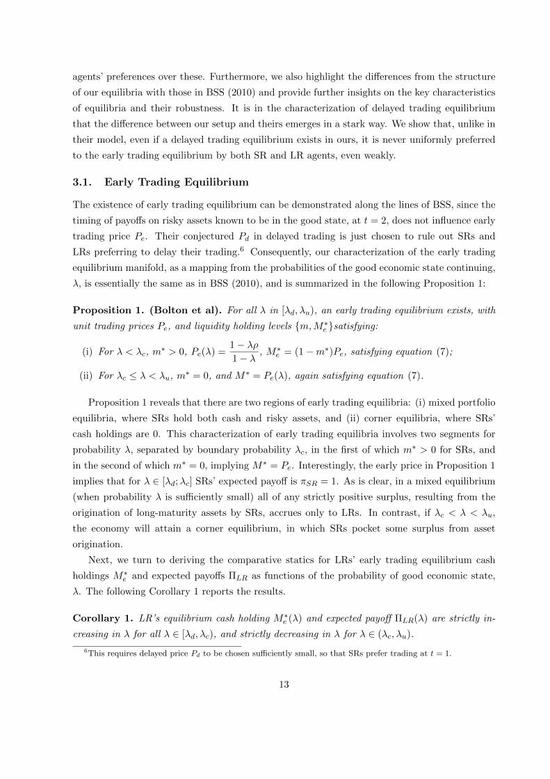
SRs investment opportunity set and preferences: As shown in the event tree depicted in
Figure 1, the risky assets available to SRs may pay off ρ > 1 with probability λ at t = 1. Alter-
natively, the economy is “shocked.” In this case, a risky asset continues until t = 2 whereupon it
enters one of three states. In the good (alternatively, bad) state, which occurs with conditional
probability of qη (alternatively, q − qη), the payoff at t = 3 will be ρ (alternatively, 0). In the
neutral state, which thus occurs with conditional probability 1− q, the payoff at t = 3 is ρ with
conditional probability η or 0 with conditional probability 1 − η. The state of an asset held by
an SR at t = 2 is her private information. All probabilities are nontrivial: λ, q, η ∈ (0, 1).
To be clear, at t = 1 the state of the world with respect to all of SRs’ risky assets’ future
payoffs are common knowledge. Moreover, when economy is shocked at t = 1, risky assets’
payoffs evolve independently of one another by t = 2, and the state of any risky asset held by
an SR then becomes her private information. Since there is a continuum of SRs, there is no
aggregate uncertainty over this period. In addition, we assume that all SRs hold well diversified
portfolios of risky assets, meaning that if at t = 1 the economy is shocked then at t = 2 each SR
has a deterministic proportion of its risky assets in the good, bad, and neutral states according
8

0
0
1q
q1
1
1
0 1 2 3 t
Early trade
Delayed trade
LR information set
SR asset sales
Figure 1: The Time Line of the Events.
to the probabilities above. That is, the proportions of good, bad, and neutral assets are given
by qη, q − qη, 1− q, respectively.
SRs seek to maximize
πSR(C1, C2, C3) = C1 + C2 + δC3, (1)
where Ct is an SR’s cash flow at date t and δ ∈ (0, 1).
LRs investment opportunity set and preferences: The long term asset available to LRs has a
liquidation value of 0 at t = 1, 2 and a positive payoff at t = 3 determined by the function F (I),
where I is the amount invested. This “production function,” F , is strictly increasing, strictly
concave, and satisfies the Inada conditions. It also has F ′(K) > 1 everywhere, ensuring that
even holding minute amounts of cash involves a strict opportunity cost for LRs. In turn, this
implies that LRs would carry cash only if they would be able to buy SRs risky assets cheaply
(below its actuarially fair value) in some state(s) of the world. LRs seek to maximize
πLR(C1, C2, C3) = C1 + C2 + C3. (2)
Gains from trade: The discounting of t = 3 cash flows by SRs, but not LRs, generates
potential gains from trade at one or more of the interim dates.
The actuarially fair value of a unit of the risky asset in the shocked state at t = 1 is ηρ. The
model is set up so that this remains the actuarially fair value of the average asset in all of the
9

subsequent non-endnodes shown in Figure 1, for example, at t = 2 if an asset is in the neutral
state. However, the value of the average risky asset to an SR at any of these nodes is only δηρ.
Note that an SR’s private information at t = 2 gives rise to a potential adverse selection
problem with respect to trading at this date, which could be avoided by trading at t = 1. The
prices that will be obtained from trading at either date will have to be determined in equilibrium,
and these will depend on the equilibrium amount of cash carried by LRs.
The (securitization and) selling of the SRs investments in risky assets is central to the model.
In particular, it is assumed that
A1. λρ+ (1− λ)δηρ < 1.
A2. λρ+ (1− λ)ηρ > 1.
The first assumption (A1) implies that the expected payoff to an SR from holding the risky asset
all the way to t = 3 is less than what the SR would get from holding cash. (A2) says that the
expected payoff from the risky asset is larger than that of cash, implying that it may be socially
optimal for the risky investment to made (under the assumption that all agents are risk neutral)
if they can be transferred to LRs. To generate such trade, it is necessary that LRs opportunity
cost of holding cash is not “too large.” The precise condition we assume is stated below, [(A3)],
after we discuss trading at t = 1 versus t = 2.
Assumptions (A1) and (A2) that generate the originate and sell (securitize) feature of the
model also constrain λ to be in an interval
(λd, λu) ≡(
1− ηρ(1− η)ρ
,1− δηρ
(1− δη)ρ
). (3)
Early versus delayed trade: Denote the quantity of risky assets and the price per unit an SR
sells at t = 1 (early trade) by Xe and Pe, respectively. The corresponding notation for trade at
t = 2 (delayed trade) is Xd and Pd. Given this notation, an SR’s expected payoff can be written
πSR = m+ λ(1−m)ρ+ (1− λ){XePe +XdPd) + δ(1−m−Xe −Xd)E[ρ̃3|Φ]}, (4)
where E[ρ̃3|Φ] is the per unit expected payoff to the risky assets the SR holds to t = 3 given
the expected characteristics of these, Φ. Due to the adverse selection problem at time t = 2 the
expected characteristics Φ of assets traded at time t = 2 depend on second period price Pd. In
particular, if this price is too low then only lemons are traded and hence the expected payoff is
zero.
Private information and an associated lemons problem at t = 2 gives rise to the possibility
that an SR would hold on to her good assets when trading at t = 2. If so, (4) becomes
πSR = m+ λ(1−m)ρ+ (1− λ){XePe + (1−m−Xe)[(1− qη)Pd + qηδρ]}. (5)
10

In this case, an SR prefers trading early if and only if Pe ≥ (1 − qη)Pd + qηδρ All agents are
“small,” in the sense that they do not believe they influence market prices.
Given a preference for early trading (Pd is sufficiently low), an SR would invest in the risky
asset at t = 0 only if Pe(1− λ) + ρλ ≥ 1. Equality of these terms is required for the SR to hold
both cash and the risky asset. Given (5) and a preference for delayed trading (Pe is sufficiently
low), an SR would invest in the risky asset at t = 0 only if [Pd(1− qη) + qηδρ](1− λ) + ρλ ≥ 1.
Our analysis in subsequent sections focuses on early versus delayed trading equilibria, where
SRs invest in risky assets and, if the economy is shocked, trades either at t = 1 or at t = 2. With
δ being sufficiently large, trade is subject to adverse selection at t = 2, i.e., only bad and neutral
risky assets would be sold in it. In equilibrium, if the economy is shocked, all of an LR’s cash
holdings, M , will be used to buy risky assets. Thus, in a conjectured early trading equilibrium
(where all trade after a shock occurs at t = 1), Xe = M/Pe and so the expected payoff to an LR
is:
ΠLR = F (K −M) + λM + (1− λ)M
Peηρ. (6)
The LR optimizes by choosing M to satisfy the first order condition:
F ′(K −M∗e ) = λ+ (1− λ)ηρ
Pe. (7)
This simply says that the marginal cost to an LR of holding cash must equal the marginal return.
The optimal cash holding, M∗, is strictly positive if F ′(K) is sufficiently small:
A3. F ′(K) < λ+(1− λ)2ηρ
1− λρ.
Assumption (A3) guarantees the existence of a non-trivial early trading rational expectations
equilibrium.
Similarly, if a non-trivial delayed trading equilibrium with price Pd exists, in which SRs at
t = 2 trade not only “lemons” but also neutral assets, the ex ante expected payoff of LR agents
in it is given by:
ΠLR = F (K −M) + λM + (1− λ)1− q1− qη
M
Pdηρ, (8)
where (1 − q)/(1 − qη) is the probability of buying a neutral asset, conditional on the fact that
both bad and neutral assets are traded at t = 2. Accordingly, an LR’s first order condition in
delayed trading equilibrium is given by:
F ′(K −M∗d ) = λ+ (1− λ)(1− q)1− qη
ηρ
Pd. (9)
The asset prices are then determined from market clearing conditions that equate the demand
and supply of assets at times t = 1 and t = 2.
11

2.3. Comparison with BSS (2010)
Both models capture the idea that SRs (banks) may generate liquidity at an interim date by
selling long-term risky assets, but there may be a cost due to adverse selection when they choose
to trade at a later date, after asymmetric information about these assets has arisen.. SRs can
potentially avoid adverse selection costs by selling at the early interim date, rather than the late
interim date, before asymmetric information develops. However, this may have other costs, since
it is costly for LRs to carry cash, by way of opportunity costs arising from foregone alternative
investments in their illiquid long-term asset. Since trade at the early interim date involves a
larger portion of SRs risky assets being sold, early trade may thereby be inferior to late trade.
Thus, there is a potential tradeoff between trading early versus late that relates to a tradeoff
between adverse selection costs, and demand-side liquidity holding costs for LRs..
In their setup, BSS show that whenever both early and delayed trading equilibria exist, the
delayed trading equilibrium is Pareto superior. In our setup, this is not the case. Indeed, we
will argue below that the delayed trading equilibrium lacks robustness. This dramatic difference
in our conclusions, and thus our respective interpretations of what constitutes a crisis, as well
as how to respond to it, has its origins in our differing key assumptions. We assume that if the
economy suffers an adverse shock at t = 1, SRs’ risky assets would not pay off before t = 3. In
contrast, BSS assume that a subset of these risky assets will pay off early, i.e., become perfectly
liquid, hence completely risk-free. Specifically, they assume that a risky asset pays off ρ at t = 2
if it is in the good state. In our setup, the payoff of ρ will not occur immediately, but at t = 3.
This is a short-cut to a more realistic assumption, whereby some residual risk of a lower payoff
will remain for this subset, which would reduce the payoff to SRs holding on to these.
This seemingly minor difference impacts crucially the tradeoff between adverse selection ver-
sus liquidity holding costs that is at the heart both models. In BSS (2010), the analysis and
results on early versus delayed trading are determined by LRs’ comparative costs of investing in
liquid assets, to support the long-term equilibrium asset prices in these two markets. In contrast,
in our setup we allow for the possibility of adverse selection at t = 2 giving rise to a deadweight
cost for SRs, namely their payoff loss from holding onto those risky assets that are deemed to
be in the good state at t = 2, something that is absent in BSS (2010). Thus, our setup contains
an additional benefit from early trading, before adverse selection related issues arise. In our
analysis, we will trace out how this affects the results. It turns out that the impact is significant,
and leads to an alternative view of financial crises.
3. Early vs Delayed Equilibrium: Descriptions and Comparisons
In this Section we proceed to describe both early and delayed trading equilibrium, and charac-
terize the conditions under which one or the other should be expected to arise, depending on
12
agents’ preferences over these. Furthermore, we also highlight the differences from the structure
of our equilibria with those in BSS (2010) and provide further insights on the key characteristics
of equilibria and their robustness. It is in the characterization of delayed trading equilibrium
that the difference between our setup and theirs emerges in a stark way. We show that, unlike in
their model, even if a delayed trading equilibrium exists in ours, it is never uniformly preferred
to the early trading equilibrium by both SR and LR agents, even weakly.
3.1. Early Trading Equilibrium
The existence of early trading equilibrium can be demonstrated along the lines of BSS, since the
timing of payoffs on risky assets known to be in the good state, at t = 2, does not influence early
trading price Pe. Their conjectured Pd in delayed trading is just chosen to rule out SRs and
LRs preferring to delay their trading.6 Consequently, our characterization of the early trading
equilibrium manifold, as a mapping from the probabilities of the good economic state continuing,
λ, is essentially the same as in BSS (2010), and is summarized in the following Proposition 1:
Proposition 1. (Bolton et al). For all λ in [λd, λu), an early trading equilibrium exists, with
unit trading prices Pe, and liquidity holding levels {m,M∗e }satisfying:
(i) For λ < λc, m∗ > 0, Pe(λ) =
1− λρ1− λ
, M∗e = (1−m∗)Pe, satisfying equation (7);
(ii) For λc ≤ λ < λu, m∗ = 0, and M∗ = Pe(λ), again satisfying equation (7).
Proposition 1 reveals that there are two regions of early trading equilibria: (i) mixed portfolio
equilibria, where SRs hold both cash and risky assets, and (ii) corner equilibria, where SRs’
cash holdings are 0. This characterization of early trading equilibria involves two segments for
probability λ, separated by boundary probability λc, in the first of which m∗ > 0 for SRs, and
in the second of which m∗ = 0, implying M∗ = Pe. Interestingly, the early price in Proposition 1
implies that for λ ∈ [λd;λc] SRs’ expected payoff is πSR = 1. As is clear, in a mixed equilibrium
(when probability λ is sufficiently small) all of any strictly positive surplus, resulting from the
origination of long-maturity assets by SRs, accrues only to LRs. In contrast, if λc < λ < λu,
the economy will attain a corner equilibrium, in which SRs pocket some surplus from asset
origination.
Next, we turn to deriving the comparative statics for LRs’ early trading equilibrium cash
holdings M∗e and expected payoffs ΠLR as functions of the probability of good economic state,
λ. The following Corollary 1 reports the results.
Corollary 1. LR’s equilibrium cash holding M∗e (λ) and expected payoff ΠLR(λ) are strictly in-
creasing in λ for all λ ∈ [λd, λc), and strictly decreasing in λ for λ ∈ (λc, λu).
6This requires delayed price Pd to be chosen sufficiently small, so that SRs prefer trading at t = 1.
13

Proof: see Appendix.
The co-movement of the unit asset prices Pe(λ), and LR money holdings M∗e (λ), across the
set of early trading equilibria when λ is in [λd, λc), may well be thought of as the inverse of
“cash in the market pricing” (see Shin (2009) for its exposition), in that unit asset prices, and
external (LR) liquidity holdings held in the anticipation of buying these assets, move in opposite
directions as a function (1 − λ), the probability of such a shock. The reason, of course, is that
m∗ decreases, and hence the quantity of the long- maturity asset supplied by SRs, (1 − m∗),increases strictly in λ, i.e., as the probability of the adverse aggregate shock decreases. However,
SRs gain nothing all from that enhanced surplus!
3.2. Delayed Trading Equilibrium
In this Subsection we explore the nature of delayed trading equilibria in our economy and demon-
strate that they are substantially different from those in BSS (2010). In contrast to BSS (2010),
it turns out that there exists no set of commonly conjectured prices {Pe, Pd} such that both the
sellers (SRs) and the buyers (LRs) would prefer delayed over early trading, even weakly. Con-
sequently, we characterize delayed trading equilibria in a setting where SRs decide the timing
of trades. Specifically, a delayed trading equilibrium arises when SRs prefer delaying trading,
in which they plan to offer a proper subset of their assets to the market only at date t = 2,
irrespective of LRs’ preferences. Anticipating such a strategy of SRs, we initially assume that
LR investors have no other choice, but to trade in such a delayed equilibrium. Later, we shall
consider the possibility of strategic bilateral trading offers by LRs, at earlier stages.
Before we proceed further, we rule out an uninteresting case of pooled delayed trading equi-
librium, in which SRs sell all of their assets regardless of quality, by assuming that their discount
parameter δ is such that:
A4. δ > η.
On one hand, the delayed equilibrium price Pd cannot exceed the actuarially fair value of ηρ
for LRs to be willing to buy. On the other hand, the value of holding onto a good asset to an
SR is δρ, if he does not sell them. Consequently, assumption (A4) guarantees that δρ > Pd, and
hence SRs strictly prefer not to sell any good assets in equilibrium. Thus, our focus, as in Bolton
et al, is on non-trivial delayed trading equilibria, in which just neutral and bad assets are both
sold. SRs are willing to sell their neutral assets provided
Pd ≥ ηρδ. (10)
This condition is needed to get them to invest in the risky asset in the first place.
We now demonstrate why a BSS (2010) type of delayed trading equilibrium, in which both
SR and LR agents prefer to trade at t = 2, breaks down in our modification of their setup. Let
14

P1 be the conjectured t = 1 price in an early equilibrium, so that SRs prefer to trade at t = 2.
SRs’ objective function in (5) implies that trading at date t = 2 will be preferred whenever price
P1 is sufficiently low, so that the following inequality is satisfied:
P1 < qηρδ + (1− qη)Pd. (11)
Similarly, the LRs objective function implies that LRs would prefer to trade at t = 2 if their
expected return from trading at t = 2, conditional on both neutral and bad assets being traded
at t = 2, exceeds the expected return from an early trade. Similarly to BSS (2010) this leads to
the following condition:(1− q)ηρ
(1− qη)Pd≥ ηρ
P1, (12)
where (1− q)/(1− qη) is the conditional probability of buying a neutral asset at t = 2 given that
inequality (10) is satisfied, and hence both bad and neutral assets are traded at t = 2. It can
easily be verified that inequalities (10)–(12) cannot hold simultaneously, and hence, there is no
delayed equilibrium in which both SRs and LRs would prefer to trade at t = 2. Indeed, the last
inequality implies that (1− q)P1 ≥ (1− qη)Pd, which in conjunction with (11) yields P1 < ηρδ.
The two latter inequalities (1−q)P1 ≥ (1−qη)Pd and P1 < ηρδ then jointly imply that Pd < ηρδ,
which contradicts inequality (10) guaranteeing that neutral assets are traded at t = 2. Thus, we
have proven the following Lemma.
Lemma 1. In a delayed trading equilibrium (where conjectured P1 is sufficiently low, so that
SRs prefer trading at t = 2), an LR would actually prefer trading early as this would earn her a
strictly higher rate of return.
This opposing preferences for the timing of trades is a very significant departure, in terms of
results, from BSS (2010). It is driven by our assumption that after the economy experiences
an adverse aggregate shock, even assets that turn out to be good do not become fully liquid
(implicitly risk-free). We model this difference via assuming that assets which SRs know to be
(relatively) good (better) at t = 2, do not pay off before t = 3, making it costly for them to
hold on to these. In contrast, in BSS (2010) there is a range of examples, involving SRs choosing
strictly positive money holdings m∗ > 0 in both early and delayed trading equilibrium, and thus
being indifferent vis-a-vis their payoffs across the two, in which the LR agents strictly prefer
to trade later, benefiting from being able to buy a proper subset of a greater quantity of SR
investment in the long-maturity assets in the delayed equilibrium, at a relatively advantageous
price.
Given Lemma 1 above, the only case in which a delayed trading equilibrium could arise in our
setup is one where SR agents perceive that they will be strictly better off in such an equilibrium,
as compared to an early trading equilibrium. As a result, they withhold their supply of the long-
maturity asset from its market, until it is common belief that they have asymmetric information
15

about subsets of their portfolio, and would only be selling their average and bad quality assets.
In general, such a delayed equilibrium will be supported by a wide range of prices P1 satisfying
inequality (11). However, it is reasonable to consider only refined equilibria, where P1 coincides
with a pertinent early trading equilibrium price, which reflects SRs’ belief that their deviation
from a delayed trading strategy will result in an early trading equilibrium outcome. The following
Lemma allows us to impose further restrictions on the set of plausible delayed trading equilibria.
Lemma 2. SRs would never strictly prefer a Delayed trading equilibrium in which m∗ > 0, over
any early trading equilibrium. Such a delayed equilibrium would also make LR agents strictly
worse off than in early trading - unlike as in BSS (2010).
Lemma 2 can easily be established by simply comparing the expected payoffs across the
two equilibria. An important implication of this Lemma is that it prompts us to look only
for delayed equilibria which entail m∗ = 0 for SRs, since otherwise SRs will be better off by
switching to an early equilibrium. For example, consider a set of parameters such that an early
trading equilibrium, described in Proposition 1 above, entails money holdings m∗ > 0 by SR
agents, whereas delayed equilibrium entails m∗ = 0 for SRs. As noted in the discussion following
Proposition 1, SR agents’ payoff in such an early equilibrium would be equal to πSR = 1, and
hence be no more than if she had invested only in the liquid asset, setting m = 1. In contrast, in a
delayed equilibrium with m∗ = 0, in which SRs invest all of their endowment in the long-maturity
asset, their expected payoff from so doing, [λρ + (1 − λ){qηδρ + (1 − qη)Pd}], must necessarily
strictly exceed the unit payoff from just holding the liquid asset, despite gains from trade given
up (to the detriment of LR agents’ payoffs) by SRs planning not to trade their better quality
asset subsets.
To start with, we derive a necessary condition for the existence of a delayed trading equi-
librium with m∗ = 0, wherein SRs expect to get price Pe(λ) = (1 − λρ)/(1 − λ) – the price
in an early trading equilibrium with m∗ > 0 – if they would deviate to trading early. SRs
would strictly prefer to trade in such a delayed trading equilibrium, as compared to any early
equilibrium involving m∗ > 0. This leads to an economically intuitive and interpretable condi-
tion, under which a non-trivial delayed trading equilibrium could conceivably exist. Then, we
strengthen this condition, by deriving necessary and sufficient conditions for the existence of a
delayed trading equilibrium. In the process, we derive tractable upper and lower bounds on the
set of exogenous model parameters, under which an unique delayed trading equilibrium with
these desired properties must exist.
In any non-trivial delayed equilibrium with Pd ≥ δηρ, SRs would only trade a proportion
(1− qη) of their long-maturity assets about which they get either bad or neutral news. To buy
these assets at the market clearing price Pd, LR investors would have to hold Md = (1 − qη)Pd
in liquid assets, on which they obtain the expected return of [λ + (1 − λ)(1− q)ηρ/(1− qη)Pd].
16
From LRs’ optimization we then obtain the following first order condition for the optimal choice
of Md in liquid assets:
F ′(K −Md) = λ+ (1− λ)(1− q)ηρ
(1− qη)Pd> 1. (13)
Combining the above inequality with the non-triviality condition Pd ≥ δηρ, we see that for any
λ it must be true that:
δ <1− q1− qη
< 1. (14)
In addition, a consistent equilibrium price Pd must be such that SR agents strictly prefer to trade
in the delayed equilibrium, rather than coordinating on an early one:
Pe(λ) =1− λρ1− λ
≤ qηδρ+ (1− qη)Pd(λ), (15)
where we have assumed that λ < λc, so that the early trading equilibrium entails m∗ > 0 (see
Proposition 1). Combining the conditions (14) and (15) above, we can derive the following
Lemma which gives a necessary condition for the existence of a delayed trading equilibrium with
m∗ = 0:
Lemma 3. Define the “social surplus” per unit of the SR-created long-maturity asset,
S(λ) = [λρ+ (1− λ)ηρ− 1]. (16)
A necessary condition for the existence of a delayed trading equilibrium with m∗ = 0 is
S(λ) ≥ (1− λ)q21− η1− qη
ηρ. (17)
Proof: see Appendix.
Under the maintained hypothesis that λ < λc, this necessary condition creates the possibility
of a lower bound λ∗, 0 < λ∗ < λc, such that the selected equilibrium would entail early trading
for all λ < λ∗, and delayed trading for λ > λ∗. The results of Lemma 3 are further strengthened
in Proposition 2 below, which provides both necessary and sufficient conditions for the existence
of a delayed trading equilibrium with m∗ = 0 when the investors expect to trade at the early
equilibrium price Pe(λ) if they deviate and trade early. While the derivation of Lemma 3 assumes
that λ < λc, and hence m∗ > 0 in the early trading equilibrium, the results of Proposition 2 hold
more generally, even in the region of λc ≤ λ ≤ λu when m∗ = 0 in the early trading equilibrium,
if SRs switch to trading early (see Proposition 1).
Proposition 2. Condition (17) above, together with the condition in inequality (19) below, are
necessary and sufficient for the existence of a delayed trading equilibrium in which m∗, the liquid
asset holdings of the selling SR agents, equals zero. Defining:
Pmin =Pe(λ)
1 + q(1− η), (18)
17

F ′(K − (1− qη)Pmin) <[λ+ (1− λ)
(1− q)ηρ(1− qη)Pmin
]. (19)
Moreover, there exist upper and lower bounds on δ, given by:
δ∗(λ) =x
ηρ, δ∗(λ) = max
{xρ,Pe(λ)− (1− qη)x
qηρ
}, (20)
where x solves a nonlinear equation
F ′(K − (1− qη)x) = λ+ (1− λ)ηρ(1− q)(1− qη)x
, (21)
such that for all pairs {λ, δ} ∈{{λ, δ} : δ∗(λ) ≤ δ ≤ δ∗(λ)
}there exists a unique delayed
equilibrium with m∗ = 0 and price Pd = x ≥ Pmin which SRs prefer to an early equilibrium
with price Pe(λ). Furthermore, the length of the equilibrium existence interval on δ satisfies the
following inequality:
δ∗(λ)− δ∗(λ) < min{
1− η, 1− qq
}. (22)
Proof: See the Appendix.
Proposition 2 establishes necessary and sufficient conditions for the existence of a unique
delayed trading equilibrium and provides a tractable characterization of the equilibrium existence
regions. It also establishes a lower bound on the equilibrium price Pd, given by (18), which
guarantees that the equilibrium price is high enough to induce SRs to choose to trade late and
supply not only the lemons but also average quality assets. The existence region is characterized
in terms of upper and lower bounds (20) on the discount parameter δ. Intuitively, on one hand,
parameter δ should be sufficiently high to induce the SRs to trade at t = 2, so that they get a
higher total expected discounted payoff, despite holding onto the subset of assets on which they
receive good news at t = 1. On the other hand, it cannot be too high since otherwise Pd ≥ δηρ
is violated and hence only lemons are traded in the market. Consequently, the equilibrium exists
only for δ in an intermediate range, bounded by some δ∗ and δ∗.
The results of Proposition 2 indicate that the bounds on parameter δ become tighter as η or
q increases. To understand the intuition we note that as η increases a good outcome becomes
more likely in the no-news state at t = 2. Therefore, for the delayed trade to be an equilibrium
outcome, SRs with no news should be more impatient to be willing to sell the asset at time t = 2.
Consequently, the upper bound δ∗ should decrease leading to the shrinkage of the interval for δ
supporting the delayed equilibrium. Furthermore, the interval for δ shrinks as q increases. The
reason is that higher q makes the no-news state less likely, increasing the proportion of lemons
traded at t = 2. Consequently, price Pd decreases, and the no-news SRs should be more impatient
(as measured by their δ) to sell assets at t = 2, and hence δ∗ should decrease reaching zero in
the limit.
18
From the results of Proposition 2 it can additionally be demonstrated that SRs prefer a
delayed equilibrium with m∗d = 0 to an early one with m∗e = 0 or m∗e > 0, so that πd ≥ πe, where
expected payoffs πd and πe are given by:
πd = λρ+ (1− λ)(qηρδ + (1− qη)Pd), (23)
πe = m∗e + (1−m∗e)(λρ+ (1− λ)Pe). (24)
Consequently, the SRs choose to trade late, enforcing the delayed equilibrium.
To facilitate our numerical (calibration) analysis below, from Proposition 1 we observe that
the early equilibrium price Pe, required for construction of the bounds δ∗ and δ∗, can conveniently
be written as follows:
Pe(λ) = max{1− λρ
1− λ, y}, (25)
where y solves a nonlinear equation:
F ′(K − y) ={λ+ (1− λ)
ηρ
y
}. (26)
Indeed, it follows from Proposition 1 that:
Pe(λ) =
1− λρ1− λ
, if m∗e > 0,
y(λ), if m∗e = 0.
(27)
Moreover, from Proposition 1, M∗e < Pe when m∗e > 0, and hence from the first order condition
(6) and concavity of function F (·) it follows that F ′(K−Pe) ≥ λ+(1−λ)ηρ/Pe. Consequently, in
the early equilibrium with m∗e > 0 it can easily be demonstrated that Pe = (1−λρ)/(1−λ) ≥ y,
giving rise to expression (25). Expressions (20) for the bounds δ∗ and δ∗ along with expression
(25) for the price in the early equilibrium allow for an efficient numerical computation of the
existence regions for delayed and early equilibria, which we describe in the next subsection.
3.3. Numerical Analysis
In this subsection we numerically explore the existence regions for different equilibria in {λ, δ}-space, payoffs aggregated across SRs and LRs in different equilibria, and other relevant economic
quantities. In particular, we are interested in the regions where the delayed equilibrium with
m∗d = 0 is preferred by SRs to early equilibrium with either m∗e > 0 or m∗e = 0. Our construction
of these regions is based on the bounds for discount parameter δ derived in Proposition 2. In
addition to bounds δ∗ and δ∗, we also note that assumption (A1) imposes the following upper
bound on δ:
δ ≤ δ̄(λ) =1− λρ1− λ
1
ηρ. (28)
From the results of Proposition 1 we note that (28) along with assumption (A3) are enough to
guarantee the existence of an early equilibrium.
19

For our numerical analysis we pick the following specification for LR investment technology,
satisfying all the conditions in Section 2:
F (I) =K1−αIα
α, (29)
where α ∈ (0, 1). Given the concavity of F (·) it can easily be demonstrated that the nonlinear
equations (21) and (26) have unique solutions x and y in terms of which the early Pe and delayed
Pd equilibrium prices are derived. We calculate x and y numerically, and by substituting them
into expressions (20) obtain the upper and lower bounds for δ as functions of λ.
The characterization of the existence regions in Proposition 2 allows us to calculate the lower
bound λ∗ for the benign state probability λ, such that the delayed equilibrium with m∗ = 0 exists
(for some δ) whenever λ ≥ λ∗. The discussion in Proposition 2 implies that λ∗ can be obtained as
a solution to equation δ∗(λ∗) = δ∗(λ∗). Similarly, the expression for the early equilibrium price
Pe in (25) can be employed to characterize the “switching point” λc, introduced in Proposition
1, which separates early equilibria with m∗ > 0 (when λ < λc) and early equilibria with m∗ = 0
(when λ ≥ λc). In particular, it can easily be demonstrated that parameters λ∗ and λc solve the
following equations:
x(λ∗) =Pe(λ∗)
1 + q(1− η),
y(λc) =1− λcρ1− λc
,
(30)
where x and y in turn solve equations (21) and (26), and price Pe(λ) is given by (25).
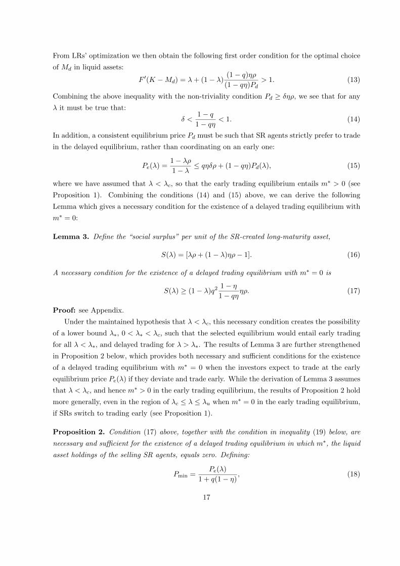
Figure 2 shows the existence regions for delayed and early equilibria in {λ, δ}-space. For
the numerical calculations we use the following set of parameters: K = 2, ρ = 1.2, η = 1/ρ,
q = 0.3, α = 0.87 (left Panel) and α = 0.925 (right Panel). The existence region for the delayed
equilibrium with m∗d = 0 is the region bounded from above by δ∗(λ) and δ̄(λ) and from below
by δ∗(λ). The early equilibrium exists for all parameters λ and δ such that δ ≤ δ̄(λ), and λc
separates the equilibria with m∗e > 0 (when λ < λc) and the equilibria with m∗e = 0 (when
λ ≥ λc). One could argue that Assumption(A1) is in some sense inessential, in that gains from
trade between SRs and LRs arising from from securitization would clearly exist even without it.
Dropping it would clearly serve to increase the size of the region in which SRs would prefer to
trade in a delayed over an early equilibrium.
The numerical calculations demonstrate that the existence regions for the delayed and early
equilibria overlap, and λ∗ < λc. Moreover, bounds δ∗(λ) and δ∗(λ) turn out to be decreasing
functions of the good state probability λ. To explain this result, we note that the delayed price
Pd = x, where x solves equation (21), is a decreasing function of λ, which can be established by
differentiating equation (21) and showing that ∂x/∂λ < 0. Intuitively, as probability λ increases,
a bad shock at t = 1 becomes less likely. Since the SRs trade only conditional on observing the
bad state at t = 1, ex ante at t = 0 the probability of trade after t = 0 goes down. Therefore, LRs
20

face higher opportunity cost of holding liquidity M , and thus prefer to invest more in their long-
term, and illiquid, technology. Consequently, conditional on a bad shock at t = 1, SRs will face
lower demand for their assets both in early and delayed equilibria, and hence both the delayed
and early prices are decreasing functions of λ, which also translates into decreasing bounds for δ.
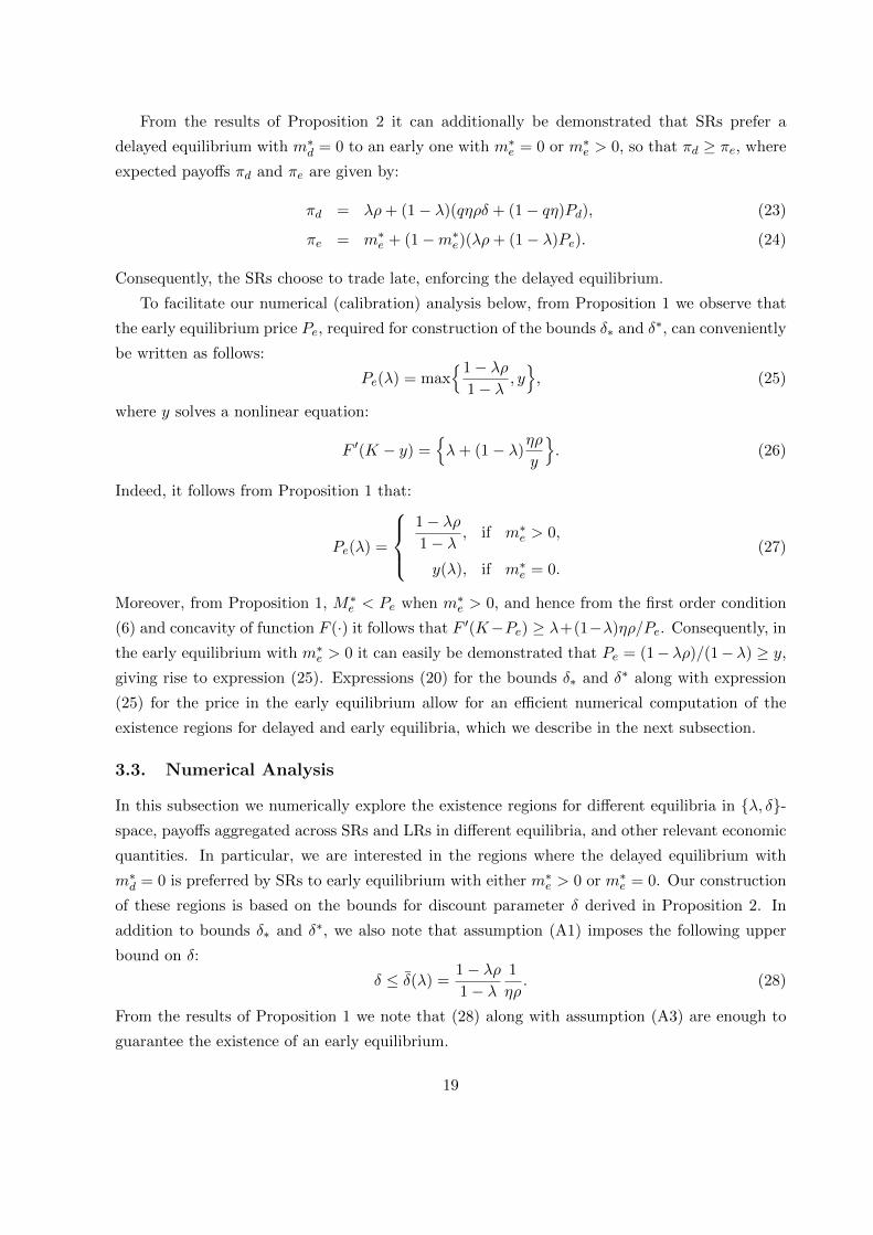
The delayed equilibrium coexists with the early equilibrium with m∗e > 0 when λ ∈ [λ∗, λc]
and with the early equilibrium with m∗e = 0 when λ ≥ λc. The size of [λ∗, λc] interval depends
on the curvature of the technology function, −F ′′(I)I/F ′(I) = 1 − α, parameterized by α. To
investigate the sensitivity of the size of this region with respect to α we numerically calculate λ∗
and λc as functions of α. Figure 3 presents the results of the calculations and demonstrates that
the size of the region decreases as parameter α goes up.
We now investigate the welfare implications of our analysis. Given the significant overlap
of the existence regions it becomes important to compare the aggregate welfare across different
equilibria. We quantify the aggregate welfare by an expected total payoff defined as the sum of
the expected payoffs of LRs and SRs, denoted by Π and π, respectively. The expected payoffs of
SRs are given by expressions (23) and (24) whereas for LRs the expected payoffs in delayed and
early equilibria take the following form:
Πd = F (K −Md) + λMd + (1− λ)M
Pd
1− q1− qη
ηρ, (31)
Πe = F (K −Me) + λMd + (1− λ)M
Peηρ. (32)
Figure 4 shows aggregate welfare in delayed and early equilibria for the model parameters K = 2,
ρ = 1.2, η = 1/ρ, q = 0.3, δ = 0.74, α = 0.87 (left Panel) and α = 0.925 (right Panel).
The aggregate welfare functions are increasing in probability λ. Moreover, the aggregate
welfare in the early equilibrium exceeds that in the delayed equilibrium for each level of the
parameter λ. To understand the economic intuition we note that SRs can have higher expected
payoff in the delayed equilibrium with m∗d = 0 than in early equilibrium. However, according
to Lemma 2 they can not have strict preference for a delayed equilibrium with m∗d > 0 over an
early equilibrium. Therefore, in a neighborhood of λ∗, their welfare will be almost unchanged by
switching from an early to a delayed equilibrium. Furthermore, according to Lemma 1, LRs are
always strictly better off in the early trading equilibrium, and hence, at least in the neighborhood
of λ∗ the aggregate welfare must be higher in the early equilibrium, a result which holds globally.
In the region where λ > Max(λ∗, λc), the intuition is again clear-cut; the non-realization of
potential gains from trading the good assets in a Delayed equilibrium must hurt LRs’ payoffs
more than it augments SRs’ payoffs, relative to these in an Early trading equilibrium for the
same parameters, by the Axioms of Revealed Preference.
21

Figure 2: Existence Regions for Early and Delayed Equilibria.
This Figure shows the existence regions for early and delayed trading equilibria for parameters K = 2,
ρ = 1.2, η = 1/ρ, q = 0.3, α = 0.87 and α = 0.925. The delayed equilibrium with m∗ = 0 exists for all
{λ, δ} such that δ∗ ≤ δ ≤ δ∗, λ∗ ≤ λ ≤ 1/ρ. The early equilibrium with m∗ > 0 exists for all {λ, δ} such
that δ ≤ δ∗e and 0 < λ ≤ λc, and the early equilibrium with m∗ > 0 exists for all {λ, δ} such that δ ≤ δ∗eand λc ≤ λ ≤ 1/ρ.
0.4 0.5 0.6 0.70.7
0.72
0.74
0.76
0.78
0.8
0.82
0.84
0.86
0.88
Equilibrium Existence Regions, = 087
c*
∗
∗
∗
0.3 0.4 0.50.85
0.855
0.86
0.865
0.87
0.875
0.88
0.885
0.89
0.895
0.9
Equilibrium Existence Regions, = 0925
c*
∗
∗
∗
Figure 3: Equilibrium λ∗ and λc as Functions of Curvature Parameter α.
This Figure plots parameters λ∗ and λc as functions of curvature parameter α for parameters K = 2,
ρ = 1.2, η = 1/ρ, q = 0.3. Delayed equilibria with m∗ = 0 and early equilibria with m∗ > 0 coexist if
λ∗ < λ < λc, while delayed equilibria withm∗ = 0 and early equilibria withm∗ = 0 coexist if λc ≤ λ ≤ 1/ρ.
0 0.1 0.2 0.3 0.4 0.5 0.6 0.7 0.8 0.90
0.1
0.2
0.3
0.4
0.5
0.6
0.7
0.8
Equilibrium ∗ and
∗
22

Figure 4: Aggregate Welfare Across Early and Delayed Equilibria.
This Figure shows the aggregate welfare in delayed and early equilibria for parameters K = 2, ρ = 1.2,
η = 1/ρ, q = 0.3, and δ = 0.74 for two cases: α = 0.87 and α = 0.925. Πe + πe is the aggregate welfare
of LRs and SRs in early equilibrium while Πd + πd is the aggregate welfare of LRs and SRs in delayed
equilibrium.
0.4 0.5 0.6 0.7 0.8 0.9 13.28
3.3
3.32
3.34
3.36
3.38
3.4
3.42
3.44
3.46
3.48
Π+
Welfare Comparison Across Delayed and Early Equilibria, = 087
Π +
Π +
0.2 0.3 0.4 0.5 0.6 0.7 0.8 0.9 13.1
3.15
3.2
3.25
3.3
3.35
Π+
Welfare Comparison Across Delayed and Early Equilibria, = 0925
Π +
Π +
Figure 5: Price Support Pe(λ∗) as Function of Curvature Parameter α.
This Figure shows the price support function Pe(λ∗) for parameters K = 2, ρ = 1.2, η = 1/ρ, q = 0.3.
0 0.1 0.2 0.3 0.4 0.5 0.6 0.7 0.8 0.9 10.4
0.5
0.6
0.7
0.8
0.9
1
1(∗)
Minimal Price Support 1(∗)
= 11
= 115
= 12
Finally, Figure 5 shows Pe(λ∗) as a function of the parameter α for different levels of return
ρ, while the other parameters are as for the previous graphs. It turns out that this function is an
increasing function of the parameter α, as well as the return ρ. As demonstrated in the subsequent
23

part of the paper, Pe(λ∗) can be thought of as a government (resale, or equity injection) Price
Support that induces “exuberant” SRs to switch to an early trading equilibrium, augmenting
overall surplus.
4. Strategy-Proofness, and Immediate Trading
We now further scrutinize the notion of delayed equilibrium we developed in Section 3. In the
Introduction, we discussed some real-life evidence in support of the existence of delayed trades.
We now address the question of the strategy proofness of delayed trading equilibria. Specifically,
we demonstrate that these equilibria are not strategy-proof, in the sense that there exist Pareto
improving bilateral offers by LRs that would induce SRs to switch to an early trade, at the
margin. Next, we reconcile the evidence in favor of the existence of delayed trading with the
non-strategy-proofness of delayed trading equilibria.
This reconciliation is achieved by introducing a realistic modification of our model in which
agents are allowed to trade immediately at the initial date t = 0, and SRs can potentially disagree
on the probability of a benign economic state, λ. We provide an example which demonstrates
that such heterogeneity of beliefs results in market segmentation, whereby some agents trade
immediately at time t = 0 and others at t = 2, consistent with anecdotal accounts of the recent
financial crisis. Indeed, we believe that such immediate (pre-shock) trading as far more realistic
depiction, than early (post-shock) trading as in BSS (2010). For the latter, we need to assume
common knowledge across traders of a state, in a real-time rather than a conceptual sense, in
which the SRs have as yet gleaned no private information about subsets of their assets, even after
an adverse aggregate shock.
4.1. Immediate Trading
As we noted in the Introduction, in early 2008, even after some adverse valuation shocks to the
mortgage backed securities market had occurred, highly levered institutions such as banks and
investment banks continued to hold nearly two-thirds in value of these assets on or off their
balance sheets. This suggests strongly that not all of these SR agents were coordinating their
planned trading of these assets with LR agents, such as insurance firms and pension funds,
in an early trading equilibrium. At the same time, it also appears to be the case that such LR
agents had acquired quite significant (over one third by value) proportions of such assets, or their
tranches, from SR originators over the years 2002-2007, before an aggregate shock pertaining to
the housing market was fully perceived. It was not until mid-2007 that these shocks lead to value
declines, and downside risk recognition, on mortgage baked securities, culminating in significant
lowering of credit ratings on many of these. Since these (SR to LR) trades occurred before
the realization of an aggregate shock, this period of asset acquisitions by LRs over 2002-2007
24

most naturally maps into date t = 0 of our model. Accordingly, we label these acquisitions as
immediate trades.
Immediate trading plays no role in the BSS (2010) model. Indeed, they note that it is
strictly sub-optimal for SRs and LRs to engage in such trades in their setting. The reasoning is
simple: relative to an Early trading equilibrium, immediate trading, at a set of prices satisfying
Π(λ) = [λρ + (1 − λ)Pe] – for SRs to be indifferent between trading at t = 0 and t = 1 –
would simply serve to make LR agents worse off, by having to hold a strictly higher amount of
liquidity Md(λ) > Me(λ). As a result, any immediate trading equilibrium would result in strictly
lower origination of the tradable asset by SRs, leading to a (weakly) Pareto inferior outcome. A
similar argument applies vis-a-vis comparing a delayed to an immediate trading equilibrium in
BSS (2010) model, in which delayed trading equilibrium outcomes Pareto dominate those from
early trading.
4.2. Strategy-Proofness and Exuberance of Priors
We show below that, in the modified setting of our model, there is a clear possibility of and a a
role for immediate trading. However, given heterogeneous prior beliefs regarding the likelihood
of an (adverse) aggregate valuation shock across SR agents, not all SRs would choose to engage
in immediate trading either. That would result in the possibility of “segmented markets”, in
which more optimistic SR agents, along with LR agents with higher marginal liquidity holding
costs, would wait to trade assets in a delayed trading equilibrium instead. The reason such a
possibility arises in our setting is the following. Unlike in the BSS model, in which their delayed
trading equilibrium exhausts all feasible gains from trade across SR and LR agents, and hence
is Pareto-preferred by them to the early trading equilibrium, in our modified setup LR agents
would have strictly preferred trading early instead. Indeed, essentially because of this feature
of our analysis, it is easily shown that, being faced with the prospect of engaging in delayed
equilibrium trade, the LR agents could make herself and her SR trading partner better off at
the margin by making an offer to buy an unit of the latter’s assets early, at time t = 1, more
pertinently (see above) initially at time t = 0. In other words, our delayed trading equilibrium
notion is not “strategy-proof”. The following Proposition formalizes this intuition.
Proposition 3. Given a delayed trading equilibrium price Pd, there is always an early trade
price offer by an LR of P > qηδρ+ (1− qη)Pd - that makes both her and her SR trading partner
strictly better off, via exchanging an unit of the asset at this price.
Proof: see Appendix.
At first sight, the lack of strategy proofness of our delayed equilibrium may lead to the
conclusion that the only valid competitive price-taking equilibrium outcomes in our setup could
be those which are associated with some early trading equilibrium. We take a more pragmatic
25

view, by considering instead the possibility of Immediate trading offers, based on the same idea
as in Proposition 3 above. We do so because, as we have argued above, the common knowledge
required of agents’ information states to allow trading after an adverse aggregate shock, but prior
to any accrual of asymmetric information, is unlikely to be valid in practice. We then show, via
an extended example, that if LR agents’ offers are based on a lower estimate of λ than that of a
subset of SR agents, then the latter may not find it worthwhile to sell their assets immediately, as
compared to waiting to trade proper subsets of these at their conjectured delayed trading price
Pd. What this example does not accomplish, however, is the task of full integration of of the
extent of such immediate trading, based on bilateral offers, among some SR and LR agents, as
compared to that of others planning to trade in a delayed, price-taking, equilibrium.
Example: Consider a scenario where ρ = 1.20, ηρ = 1, α = 0.87, δ = 0.84, q = 0.3, and Pd is such
that qηδρ+ (1− qη)Pd is between 0.892 and 0.9.7 LR agents, and some SRs as well, believe that
the ex ante probability of the benign state continuing is λp = 0.35, whereas as other “exuberant”
SR agents believe that it is λo = 0.45. Both beliefs are consistent with the conjecture that SR
agents would prefer to trade in a price-taking Delayed trading equilibrium over an Early trading
one, as Pe(λp) = [1− 1.2× 0.35/(1 − 0.35)] = 0.892 < 0.9. Suppose that LR agents are willing
to offer SR agents the equivalent of an early trading price of Pe = 0.92 in their immediate offers,
amounting to offers of Π = 0.35× 1.2 + 0.65× 0.92 = 1.02. The exuberant SR agents would
prefer not to sell immediately at this price, as they conjecture that if they wait and then trade in
a Delayed equilibrium, at the price Pd, if and when the aggregate shock would occur, they would
obtain the ex ante (at t = 0) expected payoff of 0.45× 1.20 + 0.55× 0.892 = 1.03 > 1.02, their
offered immediate trading price. This would give rise to a market segmentation, in which SRs’
assets are traded at both t = 0, 2. Here, we think of the post aggregate but pre idiosyncratic
private information state t = 1, as a conceptual rather than a “real time” state, in which trading
is feasible.
5. Implications for Financial Crises, and Optimal Regulation
In this Section, building on the insights developed in the previous ones, we provide a discussion
of financial crises and the design of regulatory policies. First, we point out the importance
of leverage for the funding of securitization prior to the recent US financial crisis, and discuss
supporting evidence. Then, we enrich our tractable example on the role of exuberance in Section
4.2, by incorporating SR agents who are leveraged using short-term repurchase contracts, and
choose their leverage levels “based on” immediate trade prices available to them at t = 0. In the
7In this example λ∗ = 0.381 and for a vector λ = (0.35, 0.4, 0.45, 0.5, 0.55) the numerical values of Pd andqηδρ+ (1 − qη)Pd are given by (0.864, 0.859, 0.854, 0.847, 0.839) and (0.9, 0.896, 0.892, 0.887, 0.881), respectively.Consequently, λ = 0.35 corresponds to qηδρ+ (1 − qη)Pd = 0.9 and λ = 0.45 corresponds to qηδρ+ (1 − qη)Pd =0.892.
26

context of a simple numerical illustration, we discuss how reassessment of the probability of an
adverse valuation shock, by initially less pessimistic LR agents, may sharply decrease immediate
trading prices, leading to Runs by repo holders. Given such a run, all SR agents would attempt
to sell (most) of their assets immediately, including those who had planned to trade only a subset
of these later, as in the example in Section 4.2. The resulting selling pressure could then give
rise to (shadow) prices at which SRs would no longer like to sell their average quality assets,
unless forced to. This trading at sub-optimal (non-equilibrium) prices constitutes our definition
of crises, and we explore potential ways of preventing, or mitigating the impact of, these using
regulatory interventions.
5.1. Myopic Leverage Choices, and Crises
It is well known that the explosive growth of securitization, of (potentially) lower quality and
riskier loan-based assets, over the years of 2002-7, was funded with sharply higher, and short-term
uninsured, debt in the form of commercial paper and repo financing. It is also commonly accepted
that market doubts, about the qualities of securitized assets which served as collateral for these
loans, started accruing from early 2007, This had negative implications for market valuation of
even the higher rated (tranches of) securities. Eventually, this accumulation of bad news resulted
in significant downgrades by credit rating agencies starting in mid-2007, after which both the
interest rates paid and haircuts (margin requirements) demanded on repo financing increased,
as documented in Gorton and Metrick (2009, 2010). This process was slow in the beginning.
While sales of new securities backed by newly originated mortgage pools, to be funded with a
lower extent of repo finance, essentially ceased by late 2007, haircuts and rates on such repo
financing only crept upwards from mid-2007 until the first quarter of 2008, before accelerating
to full-fledged systemic bank/repo runs during the summer of 2008.
In the context of the calibration of our model of Delayed trading, such high and short-term
debt financing of securitized assets by SRs is not difficult to understand. In our numerical
example, SR agents who plan to trade in a Delayed equilibrium, intend to divest a proportion
1−qη, or 75 percent, of their risky investments in that market at t = 2. Hence, to the extent they
were unconstrained by regulatory capital constraints (on their “market book” for commercial
banks), it made sense to these agents to fund their holdings between origination and trading
dates, using short-term collateralized debt, rather than via augmenting their longer-term deposit
or equity bases. So, commercial banks which held on to their own, or bought from others,
higher rated tranches of securitized assets, increased their commercial paper issuance sharply.
Alternatively, they and others “sold” such risky assets to special investment vehicles (or conduits),
which obtained their funding largely with repo financing, coupled with “implicit” equity injection
promises from their sponsors.
In his magisterial review of the consequences and possible causes of the great financial crisis
27
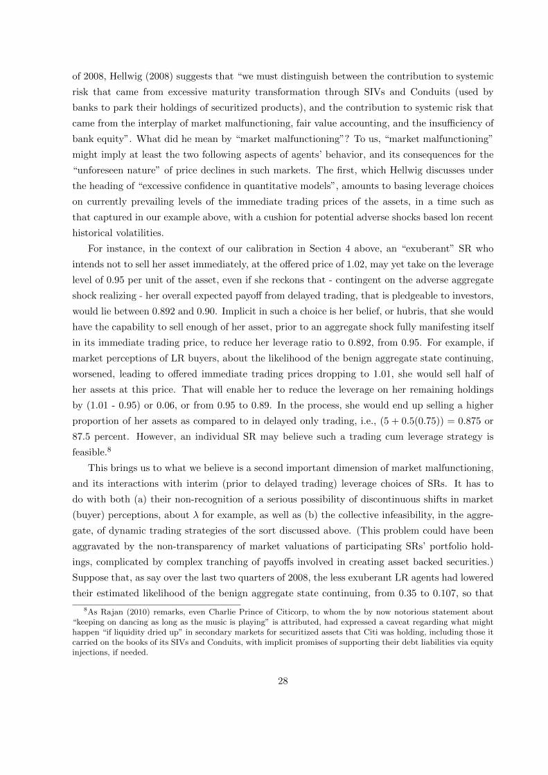
of 2008, Hellwig (2008) suggests that “we must distinguish between the contribution to systemic
risk that came from excessive maturity transformation through SIVs and Conduits (used by
banks to park their holdings of securitized products), and the contribution to systemic risk that
came from the interplay of market malfunctioning, fair value accounting, and the insufficiency of
bank equity”. What did he mean by “market malfunctioning”? To us, “market malfunctioning”
might imply at least the two following aspects of agents’ behavior, and its consequences for the
“unforeseen nature” of price declines in such markets. The first, which Hellwig discusses under
the heading of “excessive confidence in quantitative models”, amounts to basing leverage choices
on currently prevailing levels of the immediate trading prices of the assets, in a time such as
that captured in our example above, with a cushion for potential adverse shocks based lon recent
historical volatilities.
For instance, in the context of our calibration in Section 4 above, an “exuberant” SR who
intends not to sell her asset immediately, at the offered price of 1.02, may yet take on the leverage
level of 0.95 per unit of the asset, even if she reckons that - contingent on the adverse aggregate
shock realizing - her overall expected payoff from delayed trading, that is pledgeable to investors,
would lie between 0.892 and 0.90. Implicit in such a choice is her belief, or hubris, that she would
have the capability to sell enough of her asset, prior to an aggregate shock fully manifesting itself
in its immediate trading price, to reduce her leverage ratio to 0.892, from 0.95. For example, if
market perceptions of LR buyers, about the likelihood of the benign aggregate state continuing,
worsened, leading to offered immediate trading prices dropping to 1.01, she would sell half of
her assets at this price. That will enable her to reduce the leverage on her remaining holdings
by (1.01 - 0.95) or 0.06, or from 0.95 to 0.89. In the process, she would end up selling a higher
proportion of her assets as compared to in delayed only trading, i.e., (5 + 0.5(0.75)) = 0.875 or
87.5 percent. However, an individual SR may believe such a trading cum leverage strategy is
feasible.8
This brings us to what we believe is a second important dimension of market malfunctioning,
and its interactions with interim (prior to delayed trading) leverage choices of SRs. It has to
do with both (a) their non-recognition of a serious possibility of discontinuous shifts in market
(buyer) perceptions, about λ for example, as well as (b) the collective infeasibility, in the aggre-
gate, of dynamic trading strategies of the sort discussed above. (This problem could have been
aggravated by the non-transparency of market valuations of participating SRs’ portfolio hold-
ings, complicated by complex tranching of payoffs involved in creating asset backed securities.)
Suppose that, as say over the last two quarters of 2008, the less exuberant LR agents had lowered
their estimated likelihood of the benign aggregate state continuing, from 0.35 to 0.107, so that
8As Rajan (2010) remarks, even Charlie Prince of Citicorp, to whom the by now notorious statement about“keeping on dancing as long as the music is playing” is attributed, had expressed a caveat regarding what mighthappen “if liquidity dried up” in secondary markets for securitized assets that Citi was holding, including those itcarried on the books of its SIVs and Conduits, with implicit promises of supporting their debt liabilities via equityinjections, if needed.
28

their maximal price offer for immediate trading had declined to 0.107× 1.2 + 0.893× 0.92 = 0.95,
in the context of our example above. As soon as that happened, repo holders of an SR who had
taken on the leverage level of 0.95 would have started a Run, taking the immediate trading price
as the maximal liquidation value of the SR assets they had funded, as in the model of He and
Xiong (2009).9 If sufficiently many SRs, with similar leverage levels as well as absence of inside
liquidity m∗ to finance such withdrawals, then try to sell ALL of their assets immediately, that
would further lower offered prices, ultimately to a level below δηρ, at which point the secondary
market will collapse, and remain so into period t = 2, when asymmetric information about
qualities of offered assets takes hold. At best, in a more general setting, only the worst quality
assets would be voluntarily traded. The reason is, of course, that the liquidity available from
LR agents for buying these assets equals at most - because some had bought the asset earlier in
immediate trading from less exuberant SRs - the level required to support a price level of Pd,
for a volume/measure (1 − qη) units of assets to be sold in Delayed trading. It would thus not
suffice even to support the price level of Pe(λ∗), given such a Run.
5.2. Alternative Mitigating Regulatory Policies
Two major regulatory policy interventions that are natural to consider in our setting are minimum
capital, or equivalently maximum leverage, ratio restrictions, as well as minimum asset price
Guarantees, possibly coupled with restrictions on Liquidity ratiosm∗ ex ante. Let us first consider
the former. For example, a regulator may set the maximum leverage ratio on investments in the
risky technology to be Pe(λ∗) = qηδρ+ (1− qη)Pd(λ∗), in which λ∗ represents, as before, the
switch point above which SR agents would prefer the delayed over the early trading equilibrium.
Without much detailed knowledge of the LR agents’ opportunity cost function for providing
liquidity to the asset market, or F (I), this would not be an easy policy to implement: doing
so based on the lowest λ that satisfies our necessary condition in Lemma 3 above, will result
in a too generous leverage ratio, which may result in runs as above. Even if a regulator has
the informational capacity to calculate λ∗, there are still two potential difficulties. For λ > λ∗,
Pd(λ) in Delayed trading equilibrium with m∗ = 0 would be decreasing in λ, as with a set of
Early trading equilibrium with m∗ = 0, for λ > λc > λ∗, as described in Proposition 1 and
its Corollary above. On the other hand, if the regulator sets a maximum leverage ratio at the
level of say Pe(λu), that may be overly restrictive, and serve to decrease the pledgeable value to
investors arising from securitizing the assets. In any event, a maximal leverage ratio constraint
on SRs, applied also to their “off balance sheet” (effective) asset holdings, will not prevent the
planned trading strategies of at least a subset of them – all assigning probabilities λ > λ∗ to the
9If on the other hand the book Leverage Ratio chosen by Optimistic SRs were 0.99, when Offered immediatePrice was 1.02 – market debt to equity ratios of 33 were observed in 2007-8 – then relatively Pessimistic LR’slambda beliefs would only have to decline from 0.35 to 0.25, in order to cause Repo Runs by the short-term debtholders of the more optimistic SRs, as 0.25 × 1.2 + 0.75 × 0.92 = 0.99 (see He and Xiong (2009)).
29

aggregate adverse valuation shock not occurring – being delayed trading, coupled with no inside
liquidity holding (setting m = 0). As we have noted above, such delayed trading - in our model,
as opposed to that of BSS (2010) - would lead to part of the feasible gains from trade between
SR and LR agents being unrealized, decreasing (as seen in our numerical simulations) payoffs
aggregated over them.
An alternative regulatory tool, also noted in the BSS (2009, 2010) papers, would be for the
regulator – with access to fiscal or monetary powers - to provide a minimum resale price guarantee
on the risky asset. The purpose of such a guarantee in our setting would be the opposite of what
it is in the BSS setting, where it supports a delayed trading equilibrium when private liquidity
provision by LR agents, in the face of the lemons discount in pricing given adverse selection,
is insufficient for its existence. Our price guarantee will apply at Par to Immediate trading,
or to (post-shock) or Early trading at the price level Pe(λ∗). In practice, given the difficulty of
ruling out asymmetric information about the quality levels of subsets of assets held by SR agents,
especially after an adverse aggregate shock, such a guarantee may be implemented instead via
a pre-specified valuation criterion for partial equity injections. For λ < λ∗, no SR agent would
strictly prefer to sell to the regulator at these prices. Instead, they would invest and trade as in
the BSS Early trading equilibrium, with m∗ > 0, or implement an immediate trading equilibrium
with a higher level of m∗. However, in these cases, they would not be constrained by possibly
overly restrictive (see above) leverage regulations.
Indeed, now even when SR agents would believe that λ > λ∗, they would plan to sell all or
part of their securitized assets immediately to LRs, and then may later accept a partial equity
injection, after an aggregate shock. Thus, the possibility of Runs of the sort we outlined above,
associated with a delayed “cherry picking” trading strategy, would be eliminated. However, SR
agents would now invest - given the simple linear-in-payoffs expected utility functions we have
assumed - all of their funding capacity in the long-term asset, setting m∗ = 0. As a result, some
of the sales of assets being originated by SR agents would indeed be to the regulator/government,
as private external liquidity provided by LR agents would not suffice, to support a price level of
P (λ∗) for this volume of asset sales. If the regulator’s marginal cost of providing such liquidity is
no lower than that of LR agents, at the hypothetical Early equilibrium for these levels of λ, the
regulator may seek to couple is price support with a minimum liquidity ratio.10 Nevertheless, the
regulator’s overall objective function must take into account not only the costs of providing such a
price guarantee, but also the augmentation of the overall surplus arising from securitization.This
would manifest itself in the form of higher expected profit for LR agents, and it is conceivable that
taxation of that could suffice to compensate the regulator (government) for its cost of providing
10A tight one would be at m∗(λ∗) and a looser one would be at m∗(λu) provided the latter is indeed non-zero,i.e., λu < λc in Proposition 1 above. In setting the level of this minimum Liquidity ratio, optimal regulatory policywould thus need to trade off governmental (deadweight or opportunity) costs of providing asset price support,for excessive asset origination at levels of λ in the neighborhood of λ∗, versus constraining such asset originationexcessively when λ is closer to λu >> λ∗.
30

a price guarantee.
6. Discussion and Concluding Remarks
In this paper, we have emphasized the theme that “systemic” risks leading to the potential
fragility of financial intermediaries, particularly those such as commercial banks with a maturity
mismatch between their originated assets and liabilities, depends on two separate if related
issues. The first is the existence of systematic aggregate risks which remain in well-diversified
portfolios backed by bank-originated assets, which may then be securitized and sold to other less
fragile institutions and investors. The second dimension of such systemic risk has to do with
the planned trading strategies of these originating (and packaging) institutions in the process
of selling their securitized (loan) portfolios. We analyze these issues using a dynamic model,
having potentially asymmetrically informed short-run funded originators, and long-run buyers
of financial assets, as in BSS (2010). We have argued that the difference in the time structure
of payments between our paper and BSS (2010), giving rise to differential costs of holding onto
even good quality assets among the originators and potential buyers, translates into dramatically
different economic implications. In particular, in contrast to their findings, we show that the
delayed trading equilibria –involving “cherry-picking” of the best quality assets by originators,
are not robust to Pareto-improving bilateral early trade offers. We have shown that delayed
trades coupled with Immediate trades prior to any adverse aggregate shock, can nevertheless
be rationalized, in an economy with heterogeneously optimistic asset originators (sellers) and
buyers.
Our analysis has yielded new insights on financial crises, and its regulation. Specifically, we
have discussed how a crisis can arise in a setting where originating short-run funded SR agents
leverage up, via repo contracts or commercial paper, at levels related to offered immediate prices
prior to an adverse aggregate shock, though their trading strategy involves “cherry-picking”, of
trading a proper subset of their assets at a lower price later. When reassessment of the probability
of an adverse aggregate shock, by less exuberant buyer agents, leads to a run by the short-term
creditors of such SRs, the resulting (attempted) dumping of assets results in sub-optimal prices
at which at best only the worst quality assets are traded, and thereby potential insolvency
among such SR agents. We have argued that optimal regulatory policy should not only attempt
– via conservative leverage and liquidity ratio restrictions – no ensure the non-bankruptcy of
systemically (to the economy) important SRs – but also try to alter their planned trading strategy,
to one of earlier and more complete disposal of their securitized assets to investors more capable of
bearing their longer-term risks. Pre-set asset resale prices, or equity injection term guarantees,
as provided by a regulatory body with fiscal powers, can play such a prudential role. Such
measures need not be thought of only as ex post interventions, to prevent systemic spreading of
crises, with repercussions beyond immediately affected institutions because of interconnections,
31
when other prudential ex ante restrictions have failed to do so.
This reemphasis is intended to contribute to current policy debates on the reform of financial
regulation, in particular on measures such as the proposed Volcker Rule. Some seek to drasti-
cally curtail “proprietary” trading by the regulated commercial banking sector, many of whose
liabilities enjoy governmental safety net protections. Bankers in turn have argued that its imple-
mentation would greatly impede their (socially beneficial) securitization activities. Our stance
is that rather than, or in addition to, reducing “clearly speculative” trading – as in (levered)
Delayed trading by SR agents in our model above – measures that dissuade banks from doing
so voluntarily, at the occasional cost of government support, may contribute to both systemic
stability and overall surplus accruing from securitization.
Some other recent papers have also focused on scenarios which may give rise to financial
crises, in which there is nevertheless an ex ante beneficial role for the securitization of assets, for
sale to non-bank investors at an early ex ante stage. Perhaps the paper closest to ours is that of
Gennaioli, Shleifer, and Vishny (2011), in which the arrival, leading to cognizance, of an adverse
aggregate shock to future payoffs on diversified securitized assets, can lead to a systemic crisis.
There are some key differences between our papers, however. First, in their model, the ex ante
benefit from securitization arises from a high demand for (ostensibly) risk-free assets by infinitely
risk-averse investors. Originating (and packaging) institutions meet this demand by tranching
the future payoffs on their assets, into a higher priority “risk-free” tranche that they sell to these
investors, retaining the rest on their balance sheets. When doing so, neither they nor the buyers
of the sold tranches recognize the possibility of the worst of (three) possible future states. When
that possibility is (sometimes) recognized later, these investors sell assets en masse, and – in the
absence of enough other investors willing to buy these (now risky) assets – the market for these
collapses.
In our model, the possibility of such an adverse aggregate payoff shock is recognized by all
parties, with some heterogeneity in their beliefs about its likelihood, and all agents are risk-
neutral. Nevertheless, leverage choices based on asset prices prevailing before such a shock,
coupled with asymmetric information about their qualities held by their originators, may lead to
dramatic drops in their post-shock prices, which are not commensurate with the post-shock ex-
pected payoffs of the average quality asset. Hellwig (2008) notes that, based on the International
Monetary Fund’s projections of losses to the values of sub-prime mortgage-backed securities as a
whole over 2007-8. it would have taken a default rate amounting to 40-45 percent of the amounts
due on the underlying loans, to rationalize the extent of such market value losses on the average
asset. Such numbers vastly exceed the hen prevailing, or later, delinquency ratios on sub-prime
mortgages as a whole. In our opinion, without adverse selection leading to withdrawal from the
supply of a major subset of better quality securitized assets from trading, it is hard to explain
32

these magnitudes, in a world with other potential buyers such as sovereign and hedge funds.11
Diamond and Rajan (2012) build an alternative model, in which potential shocks to financial
institutions at a future date arise from higher than anticipated “liquidity” demands for early
withdrawal, at an interim date prior to the full realization of returns on their longer maturity
assets. They allow, and model, a secondary market for sales of such assets to other investors,
including other banks as well as other investors, at two dates, prior to or upon realization of
this liquidity-demand shock. They show that, when decisions regarding timing of asset sales are
taken by banks’ levered equity holders, they may refrain from selling assets early, even when
that would have met their liabilities fully, but doing so at the interim date in the event of an
adverse aggregate liquidity shock would not. They interpret this as a pre-shock market “freeze”.
However, they do not allow for pre-shock runs, by (sufficiently many) uninsured bank liability
holders holding demandable debt claims, which would have forced their banks to sell assets earlier
to meet their withdrawal demands, thus “unfreezing” this market.
In future work, we hope to provide a more complete welfare analysis of our recommended
regulatory policy, involving a pre-specified asset resale price (or equity injection terms) guarantee.
This would involve a more detailed comparison of the benefits from SRs selling much more of
their originated assets early, prior to any asymmetric information arising on these, to LR buyers,
with the (deadweight) costs to regulatory authorities of providing such a price support, which
may entail their buying the remaining unsold quantities of SR originated assets at the support
price, or providing equity injections to them. In a recent paper, Angeletos, Lorenzoni, and
Pavan (2010) have analyzed an environment in which systematic, and highly correlated, shocks
to future asset payoffs may be perceived by the sellers, but not necessarily by the buyers, of a
risky asset. The buyers also attempt to infer their expected payoff from the level of investment
in this asset by its originators, a subset of the sellers. They show that in such an environment
the level of investment, and the asset price, respond relatively more to such shocks, as compared
to conditionally independent signals also received by buyers, relative to a welfare maximizing set
of these. In this single-shot trading scenario with a homogeneous risky asset, they characterize
the optimal policy interventions to attain optimal market outcomes. Our setting above, which
allows for sheterogeneity of beliefs, as well as the possibility of trading differing subsets of assets
at different points in time, having different information sets, calls for analogous modeling.
11A similar remark applies to models based on ”Knightian uncertainty” about future asset payoffs, such asCaballero and Krishnamurthy (2008)
33

Appendix: Proofs
Proof of Corollary 1. Consider LR’s expected return on money holding M as a function of
λ, R(λ):
R(λ) = λ+ (1− λ)ηρ
Pe(λ), (a.1)
which in the segment λ in [λd, λc), in part (i) of the Proposition, implies that:
R(λ) = λ+ ηρ(1− λ)2
1− λρ. (a.2)
It is straightforward to show, via differentiation, that the right hand side of (a.2) is strictly
increasing in λ, which using LR’s optimality condition (7) yields the result.12
For the second part of the corollary, concerning the region [λc, λu) in which money holdings
m∗ of SRs equals zero, so that M∗e (λ) = Pe(λ), suppose to the contrary that M∗e (λ), and thus
Pe(λ) are (weakly) increasing in λ. But, then R(λ) would be strictly decreasing in λ, which
would contradict LRs’ optimality condition, in equation (7).
Finally, the statement that LRs’ overall expected payoff is increasing (vs decreasing) in λ
whenever M∗e (λ) is increasing (vs decreasing) in λ, is implied by the axioms of Revealed Prefer-
ence, applied to LR’s objective function, described in equation (2). Q.E.D.
Proof of Lemma 3: Conditions (15) and Pd ≥ δηρ, required for a delayed equilibrium, together
imply
S ≥ (1− λ)[(1− δ)ηρ− q(1− η)δηρ]. (a.3)
Which, upon substitution for {δ, (1−δ)} from the inequality (14), implies inequality (17). Q.E.D.
Proof of Proposition 2. We first observe that if there exists a delayed equilibrium with
m∗ = 0 then the market clearing condition implies that Md = (1 − qη)Pd. Substituting the
expression for liquidity Md into LR’s first order condition (13) in delayed equilibrium we obtain
that the price Pd in delayed equilibrium is given by Pd = (1 − qη)x, where x solves a nonlinear
equation (21).
By comparing the payoffs from early and delayed trades we obtain the following condition
guaranteeing that SRs prefer to trade late:
Pe ≤ qηρδ + (1− qη)Pd, (a.4)
where Pe denotes the early equilibrium price that the SRs expect to see if they switch to early
trade. The expression on the right-hand side of (a.8) represents the expected gain from the
delayed trade conditional on observing a bad shock at t = 1.
12It is easily shown that:dR(λ)
dλ=
[1 − η
{ (1 − λρ)2 − (1 − ρ)2
(1 − λρ)2
}]> 0.
34

Moreover, if there exists a delayed equilibrium with m∗ = 0 then Pd should satisfy the
following two inequalities:
Pd ≥ ηρδ, Pd ≤ ρδ. (a.5)
Indeed, if the first inequality in (a.9) is violated only lemons are traded at time t = 2, which
is not consistent with having a non-trivial delayed equilibrium. The second inequality in (a.9)
guarantees that the SRs receiving good news at t = 2 do not trade the assets (as discussed in
Section II). Substituting Pd = (1− qη)x into the inequalities (a.8) and (a.9) and rewriting them
as inequalities on x we obtain the following inequality:
max{ηρδ,
Pe(λ)− qηρδ1− qη
}≤ x(λ) ≤ ρδ. (a.6)
The inequality (a.10) imposes restrictions on {λ, δ} in equilibrium. Resolving the inequality
(a.10) with respect to δ we obtain an equivalent inequality:
δ∗(λ) ≤ δ ≤ δ∗(λ), (a.7)
where δ∗ and δ∗ are given in (20).
So far, the inequality (a.11) has been derived as a necessary condition for the existence of the
delayed equilibrium. However, we observe that this inequality is equivalent to inequality (a.10)
which also gives a sufficient condition for the existence of a delayed equilibrium. Indeed, x solves
a nonlinear equation (21) and Pd = x defines the price in the delayed equilibrium since all the
equilibrium conditions are satisfied. In particular, from (a.10) it follows that inequalities (a.8)
and (a.9) are satisfied, and hence under the price Pd the SRs prefer to trade late. Moreover,
noting that Md = (1− qη)Pd we rewrite the non-linear equation (21) as follows:
F ′(K −Md) = λ+ (1− λ)ηρ(1− q)
(1− qη)Pd, (a.8)
which gives the FOC for LRs. Therefore, Md defined as Md = (1 − qθ)Pd indeed gives the
optimal liquidity level chosen by LRs that anticipate the delayed equilibrium. This completes
the proof that inequality (a.11) defines both necessary and sufficient condition for the existence
of a delayed equilibrium.
The uniqueness of the delayed equilibrium follows from the properties of production function
F (·). Since F (·) is an increasing and concave function the left-hand side of the equation (21)
for x is a monotonically increasing function of x on the interval (0,K) and goes to infinity as
x→ K. On the other hand, the right-hand side of (21) is a monotonically decreasing function x
which becomes infinite when x→ 0. Therefore, there exists the unique solution of equation (21)
defining the price Pd.
We now demonstrate that the inequality (19) presents an equivalent way of rewriting the
necessary and sufficient condition for the existence of the delayed equilibrium. From the inequality
35

(a.11) on δ we observe that the necessary and sufficient condition for the existence of equilibrium
is given by the inequality δ∗(λ) ≥ δ∗(λ) which implies that there exists at least one equilibrium
pair {λ, δ} satisfying inequality (a.11). By comparing δ∗(λ) and δ∗(λ) in (20) we obtain that the
inequality δ∗(λ) ≥ δ∗(λ) is equivalent to the following inequality:
x
ηρ≥ Pe − (1− qη)x
qηρ.
Resolving the above inequality with respect to x we obtain that the necessary and sufficient
condition for the existence of the delayed equilibrium is given by x ≥ Pmin, where Pmin is defined
in Proposition 2. Thus, we obtain an exogenous lower bound Pmin on the delayed equilibrium
price. Since F ′(K− (1−qη)x) is an increasing function of x the inequality x ≥ Pmin is equivalent
to the inequality (19) in Proposition 2. Therefore, the inequality (19) gives a necessary and
sufficient condition for the existence of delayed equilibrium.
We also note that the necessary condition for the existence of a delayed trading equilibrium
(17), derived in Lemma 2, is implied by the inequality (19). To demonstrate this, we first observe
that F ′(K − (1− qη)x) > 1 by assumption. Therefore, the left-hand side of the equation (21) for
x exceeds unity. Consequently, from (21) we obtain the following upper bound on price Pd:
Pd ≤(1− q)ηρ
1− qη. (a.9)
Noting that the early equilibrium price satisfies inequality Pe ≥ (1 − λρ)/(1 − λ) allows us to
rewrite the inequality Pd ≥ Pmin as follows:
Pd ≥Pe
1 + q(1− η)≥ 1− λρ
1− λ1
1 + q(1− η). (a.10)
The inequalities (a.13) and (a.14) imply that:
1− λρ1− λ
1
1 + q(1− η)≤ (1− q)ηρ
1− qη.
After simple algebraic manipulations it can easily be demonstrated that the above inequality is
tantamount to the necessary condition (17).
Finally, we prove the inequality (22) that gives an upper bound on the size of the interval for
the discount δ that supports the delayed trading equilibrium. In particular, from the expressions
for the upper and lower bounds for δ in (20) we obtain:
δ∗ − δ∗ ≤x
ηρ− x
ρ=x
ρ
1− ηη
. (a.11)
Combining the inequality (a.15) with the inequality (a.13) we obtain:
δ∗ − δ∗ ≤(1− q)(1− η)
1− qη
=(1− q)(1− η)
1− q + q(1− η)η=
11
1−η + q1−q
≤ min{
1− η, 1− qq
}.
36

The above inequality demonstrates that the equilibrium existence region shrinks as η → 1 or
q → 1. Q.E.D.
Proof of Proposition 3. Given a Pd, the commonly held conjecture of SR and LR agents
about Delayed trading equilibrium price, at the margin an LR agents would be indifferent between
reducing her planned trade at t = 2 by an unit, and making an offer to use the liquidity freed up
to buy Pd/Po units of an SR’s asset early, at the unit price Po equalling;
Po = Pd(1− qη)
(1− q). (a.12)
The SR agent who is offered this price would be strictly better off by selling early if:
Po > qηδρ+ (1− qη)Pd, (a.13)
which holds provided
ηδρ < Pd1− qη1− q
(a.14)
Inequality (a.6) holds for Pd > δηρ, which is true of any non-trivial Delayed trading equilibrium.
In contrast, in the BSS model, the analogue of (a.6) would require that:
ηρ < Pd(1− qη)
(1− q)(a.15)
which contradicts the LR agent’s First Order Condition for optimality, in equation (13). Q.E.D.
37

References
Acharya, V., H.S. Shin, and T. Yorulmazer (2009), “Crisis Resolution and Bank Liquidity”,
NBER Working Paper 15567, forthcoming in Review of Financial Studies.
Adrian, T. and H.S. Shin (2009a), “The Shadow Banking System: Implications for Financial
Regulation”, Working Paper, Federal Reserve Bank of New York.
Adrian, T. and H.S. Shin (2009b), “Liquidity, Leverage, and Monetary Policy”, American Eco-
nomic Review 89, Papers and Proceedings.
Akerlof, G. (2010), “The Market for “Lemons”: Quality Uncertainty and the Market Mecha-
nism”, Quarterly Journal of Economics 84, 488-500.
Allen, F. and D. Gale (1995), “A Welfare Comparison of Intermediaries and Financial Markets
in Germany and the US”, European Economic Review 39, 179-209.
Angeletos, G-M., G. Lorenzoni, and A. Pavan (2010), “Beauty Contests and Irrational Exuber-
ance: a Neoclassical Approach”, Working Paper, MIT and Northwestern.
Bhattacharya, S., and G. Gale (1987), “Preference Shocks, Liquidity and Central Bank Pol-
icy”, in: W.A. Barnett and K.J. Singleton, eds., New approaches to monetary economics
(Cambridge University Press, Cambridge).
Bolton, P., T. Santos, and J. Scheinkman (2009), “Market and Public Liquidity”, American
Economic Review 89, Papers and Proceedings, 594-599.
Bolton, P., T. Santos, and J. Scheinkman (2012), “Outside and Inside Liquidity”, Quarterly
Journal of Economics, ......
Caballero, R.J., and A. Krishnamurthy, “Collective Risk Management in a Flight to Quality
Episode”, Journal of Finance 63, 2195-2229.
Chari, V.V, A. Shourideh and A. Zetlin-Jones (2010), “Adverse Selection, Reputation and
Sudden Collapses in Secondary Loan Markets”, NBER Working Paper 16080.
Diamond, D.W. and R. Rajan (2000), “A Model of Bank Capital”, Journal of Finance 55,
2431-2465.
Diamond, D.W. and R. Rajan (2012), “Fear of Fire Sales, Illiquidity Seeking, and the Credit
Freeze”, Quarterly Journal of Economics.
Downing, C., D. Jaffee and N. Wallace (2009), “Is the Market for Mortgage-Backed Securities
a Market for Lemons?”, Review of Financial Studies 22, 2457-2494.
Geanakoplos, J. (2010), “The Leverage Cycle”, NBER Macroeconomics Annual.
Gennaioli, N, A. Shleifer, and R. Vishny (2011), “A Model of Shadow Banking”, Working Paper,
Harvard and Chicago.
Gorton, G. and A. Metrick (2009), “Runs on Repos”, NBER Working Paper.
Gorton, G. and A. Metrick (2010), “Haircuts”, NBER Working Paper.
He, J. and W. Xiong (2009), “Dynamic Debt Runs,” NBER Working Paper.
38
Heider, F, M. Hierova, and C. Holthausen (2010), “Liquidity Hoarding and Inter-bank Market
Spreads: the Role of Counterparty Risk”, European Central Bank working paper.
Hellwig, M. (1998), “Banks, Markets, and the Allocation of Risks in an Economy”, Journal
Institutional and Theoretical Economics 154, 328-345.
Hellwig, M. (2008), “Systemic Risk in the Financial Sector: an Analysis of the Subprime-
Mortgage Financial Crisis”, Max Planck Institute for Research, Bonn.
Rajan, R.G (2010), “Fault Lines”, Princeton University Press.
Shin, H.S. (2009), “Securitization and Financial Stability”, Economic Journal, 118, 309-332.
Stein, J. (2012), “Monetary Policy as Financial Stability Regulation”, Quarterly Journal of
Economics, forthcoming.
39