section six soil mechanics and foundations...6.1 section six soil mechanics and foundations robert...
TRANSCRIPT
6.1
SECTION SIXSOIL MECHANICS AND
FOUNDATIONS
Robert W. DayChief Engineer, American Geotechnical
San Diego, California
6.1 INTRODUCTION
6.1.1 Soil Mechanics
Soil mechanics is defined as the application of the laws and principles of mechanicsand hydraulics to engineering problems dealing with soil as an engineering material.Soil has many different meanings, depending on the field of study. For example,in agronomy (application of science to farming), soil is defined as a surface depositthat contains mineral matter that originated from the original weathering of rockand also contains organic matter that has accumulated through the decompositionof plants and animals. To an agronomist, soil is that material that has been suffi-ciently altered and supplied with nutrients that it can support the growth of plantroots. But to a geotechnical engineer, soil has a much broader meaning and caninclude not only agronomic material, but also broken-up fragments of rock, volcanicash, alluvium, aeolian sand, glacial material, and any other residual or transportedproduct of rock weathering. Difficulties naturally arise because there is not a distinctdividing line between rock and soil. For example, to a geologist a given materialmay be classified as a formational rock because it belongs to a definite geologicenvironment, but to a geotechnical engineer it may be sufficiently weathered orfriable that it should be classified as a soil.
6.1.2 Rock Mechanics
Rock mechanics is defined as the application of the knowledge of the mechanicalbehavior of rock to engineering problems dealing with rock. To the geotechnicalengineer, rock is a relatively solid mass that has permanent and strong bonds be-tween the minerals. Rocks can be classified as being either sedimentary, igneous,or metamorphic. There are significant differences in the behavior of soil versusrock, and there is not much overlap between soil mechanics and rock mechanics.
6.2 SECTION SIX
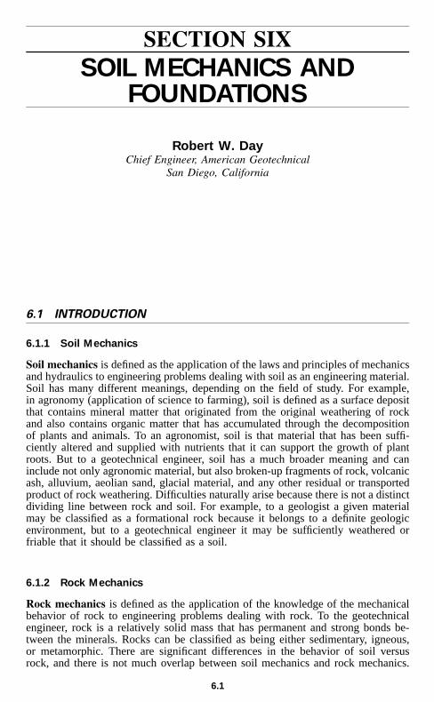
TABLE 6.1 Problem Conditions Requiring Special Consideration
Problemtype Description Comments
Organic soil, highly plasticsoil
Low strength and high compressibility
Sensitive clay Potentially large strength loss upon largestraining
Micaceous soil Potentially high compressibilitySoil Expansive clay, silt, or slag Potentially large expansion upon wetting
Liquefiable soil Complete strength loss and high deformationscaused by earthquakes
Collapsible soil Potentially large deformations upon wettingPyritic soil Potentially large expansion upon oxidation
Laminated rock Low strength when loaded parallel to beddingExpansive shale Potentially large expansion upon wetting;
degrades readily upon exposure to air andwater
Pyritic shale Expands upon exposure to air and water
RockSoluble rock Rock such as limestone, limerock, and gypsum
that is soluble in flowing and standing waterCretaceous shale Indicator of potentially corrosive groundwaterWeak claystone Low strength and readily degradable upon
exposure to air and waterGneiss and schist Highly distorted with irregular weathering
profiles and steep discontinuitiesSubsidence Typical in areas of underground mining or high
groundwater extractionSinkholes Areas underlain by carbonate rock (Karst
topography)
Negative skin friction Additional compressive load on deepfoundations due to settlement of soil
ConditionExpansion loading Additional uplift load on foundation due to
swelling of soilCorrosive environment Acid mine drainage and degradation of soil and
rockFrost and permafrost Typical in northern climatesCapillary water Rise in water level which leads to strength loss
for silts and fine sands
Source: ‘‘Standard Specifications for Highway Bridges,’’ 16th ed., American Association of StateHighway and Transporation Officials, Washington, DC.
Table 6.1 presents a list of common soil and rock conditions that require specialconsideration by the geotechnical engineer.
6.1.3 Foundation Engineering
A foundation is defined as that part of the structure that supports the weight ofthe structure and transmits the load to underlying soil or rock. Foundation engi-neering applies the knowledge of soil mechanics, rock mechanics, geology, and
SOIL MECHANICS AND FOUNDATIONS 6.3
structural engineering to the design and construction of foundations for buildingsand other structures. The most basic aspect of foundation engineering deals withthe selection of the type of foundation, such as using a shallow or deep foundationsystem. Another important aspect of foundation engineering involves the develop-ment of design parameters, such as the bearing capacity of the foundation. Foun-dation engineering could also include the actual foundation design, such as deter-mining the type and spacing of steel reinforcement in concrete footings. Asindicated in Table 6.2, foundations are commonly divided into two categories: shal-low and deep foundations.
6.2 FIELD EXPLORATION
The purpose of the field exploration is to obtain the following (M. J. Tomlinson,‘‘Foundation Design and Construction,’’ 5th ed., John Wiley & Sons, Inc., NewYork):
1. Knowledge of the general topography of the site as it affects foundation designand construction, e.g., surface configuration, adjacent property, the presence ofwatercourses, ponds, hedges, trees, rock outcrops, etc., and the available accessfor construction vehicles and materials.
2. The location of buried utilities such as electric power and telephone cables,water mains, and sewers.
3. The general geology of the area, with particular reference to the main geologicformations underlying the site and the possibility of subsidence from mineralextraction or other causes.
4. The previous history and use of the site, including information on any defectsor failures of existing or former buildings attributable to foundation conditions.
5. Any special features such as the possibility of earthquakes or climate factorssuch as flooding, seasonal swelling and shrinkage, permafrost, and soil erosion.
6. The availability and quality of local construction materials such as concreteaggregates, building and road stone, and water for construction purposes.
7. For maritime or river structures, information on tidal ranges and river levels,velocity of tidal and river currents, and other hydrographic and meteorologicaldata.
8. A detailed record of the soil and rock strata and groundwater conditions withinthe zones affected by foundation bearing pressures and construction operations,or of any deeper strata affecting the site conditions in any way.
9. Results of laboratory tests on soil and rock samples appropriate to the particularfoundation design or construction problems.
10. Results of chemical analyses on soil or groundwater to determine possibledeleterious effects of foundation structures.
6.2.1 Document Review
Some of the required information, such as the previous history and use of the site,can be obtained from a document review. For example, there may be old engi-
6.4
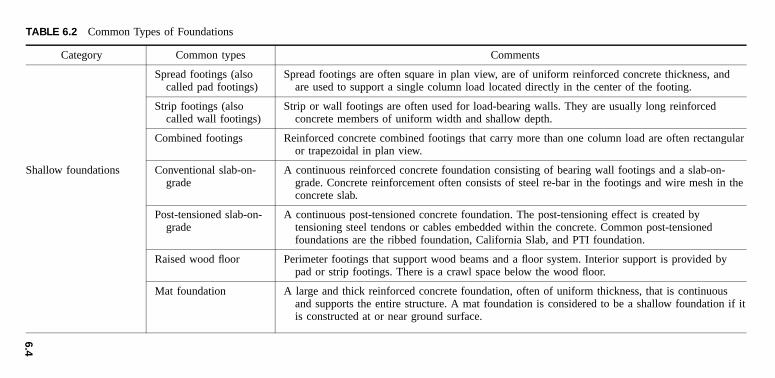
TABLE 6.2 Common Types of Foundations
Category Common types Comments
Spread footings (alsocalled pad footings)
Spread footings are often square in plan view, are of uniform reinforced concrete thickness, andare used to support a single column load located directly in the center of the footing.
Strip footings (alsocalled wall footings)
Strip or wall footings are often used for load-bearing walls. They are usually long reinforcedconcrete members of uniform width and shallow depth.
Combined footings Reinforced concrete combined footings that carry more than one column load are often rectangularor trapezoidal in plan view.
Shallow foundations Conventional slab-on-grade
A continuous reinforced concrete foundation consisting of bearing wall footings and a slab-on-grade. Concrete reinforcement often consists of steel re-bar in the footings and wire mesh in theconcrete slab.
Post-tensioned slab-on-grade
A continuous post-tensioned concrete foundation. The post-tensioning effect is created bytensioning steel tendons or cables embedded within the concrete. Common post-tensionedfoundations are the ribbed foundation, California Slab, and PTI foundation.
Raised wood floor Perimeter footings that support wood beams and a floor system. Interior support is provided bypad or strip footings. There is a crawl space below the wood floor.
Mat foundation A large and thick reinforced concrete foundation, often of uniform thickness, that is continuousand supports the entire structure. A mat foundation is considered to be a shallow foundation if itis constructed at or near ground surface.

6.5
TABLE 6.2 Common Types of Foundations (Continued)
Category Common types Comments
Driven piles Driven piles are slender members, made of wood, steel, or precast concrete, that are driven intoplace using pile-driving equipment.
Other types of piles There are many other types of piles, such as bored piles, cast-in-place piles, or composite piles.
Piers Similar to cast-in-place piles, piers are often of large diameter and contain reinforced concrete. Pierand grade beam support are often used for foundation support on expansive soil.
Caissons Large piers are sometimes referred to as caissons. A caisson can also be a watertight undergroundstructure within which construction work is carried on.
Deep foundations Mat or raft foundation If a mat or raft foundation is constructed below ground surface or if the mat or raft foundation issupported by piles or piers, then it should be considered to be a deep foundation system.
Floating foundation A special foundation type where the weight of the structure is balanced by the removal of soil andconstruction of an underground basement.
Basement-typefoundation
A common foundation for houses and other buildings in frost-prone areas. The foundation consistsof perimeter footings and basement walls that support a wood floor system. The basement flooris usually a concrete slab.
Shallow and deep foundations in this table are based on the depth of the soil or rock support of the foundation.
6.6 SECTION SIX
neering reports indicating that the site contains deposits of fill, abandoned septicsystems and leach fields, buried storage tanks, seepage pits, cisterns, mining shafts,tunnels, or other man-made surface and subsurface works that could impact thenew proposed development. There may also be information concerning on-site util-ities and underground pipelines, which may need to be capped or rerouted aroundthe project.
During the course of the work, it may be necessary to check reference materials,such as geologic and topographic maps. Geologic maps can be especially usefulbecause they often indicate potential geologic hazards (e.g., faults, landslides) aswell as the type of near-surface soil or rock at the site. Both old and recent topo-graphic maps can also provide valuable site information. Topographic maps areusually to scale and show the locations of buildings, roads, freeways, train tracks,and other civil engineering works as well as natural features such as canyons, rivers,lagoons, sea cliffs, and beaches. The topographic maps can even show the locationsof sewage disposal ponds and water tanks, and by using different colors and shad-ing, they indicate older versus newer development. But the main purpose of thetopographic map is to indicate ground surface elevations. This information can beused to determine the major topographic features at the site and for the planningof subsurface exploration, such as available site access for drilling rigs.
Another important source of information is aerial photographs, which are takenfrom an aircraft flying at a prescribed altitude along preestablished lines. Viewinga pair of aerial photographs, with the aid of a stereoscope, provides a three-dimensional view of the land surface. This view may reveal important geologicinformation at the site, such as the presence of landslides, fault scarps, types oflandforms (e.g., dunes, alluvial fans, glacial deposits such as moraines and eskers),erosional features, general type and approximate thickness of vegetation, and drain-age patterns. By comparing older versus newer aerial photographs, the engineeringgeologist can also observe any man-made or natural changes that have occurred atthe site.
6.2.2 Subsurface Exploration
In order for a detailed record of the soil and rock strata and groundwater conditionsat the site to be determined, subsurface exploration is usually required. There aredifferent types of subsurface exploration, such as borings, test pits, and trenches.Table 6.3 summarizes the boring, core drilling, sampling, and other exploratorytechniques that can be used by the geotechnical engineer.
A boring is defined as a cylindrical hole drilled into the ground for the purposesof investigating subsurface conditions, performing field tests, and obtaining soil,rock, or groundwater specimens for testing. Borings can be excavated by hand (e.g.,with a hand auger), although the usual procedure is to use mechanical equipmentto excavate the borings.
Many different types of equipment are used to excavate borings. Typical typesof borings are listed in Table 6.3 and include:
Auger Boring. A mechanical auger is a very fast method of excavating a boring.The hole is excavated by rotating the auger while at the same time applying adownward pressure on the auger to help obtain penetration of the soil or rock.There are basically two types of augers: flight augers and bucket augers. Com-mon available diameters of flight augers are 5 cm to 1.2 m (2 in to 4 ft) and ofbucket augers are 0.3 m to 2.4 m (1 ft to 8 ft). The auger is periodically removed
6.7
TABLE 6.3 Boring, Core Drilling, Sampling, and Other Exploratory Techniques*
Method(1)
Procedure(2)
Type of sample(3)
Applications(4)
Limitations(5)
Auger boring, ASTM D1452
Dry hole drilled with handor power auger; samplespreferably recovered fromauger flutes
Auger cuttings, disturbed,ground up, partially driedfrom drill heat in hardmaterials
In soil and soft rock; toidentify geologic units andwater content above watertable
Soil and rock stratificationdestroyed; sample mixedwith water below thewater table
Test boring, ASTM D 1586 Hole drilled with auger orrotary drill; at intervalssamples taken 36-mm(1.4-in) ID and 50-mm (2-in) OD driven 0.45 m (1.5ft) in three 150-mm (6-in)increments by 64-kg (140-lb) hammer falling 0.76 m(30 in); hydrostaticbalance of fluidmaintained below waterlevel
Intact but partially disturbed(number of hammer blowsfor second plus thirdincrement of driving isstandard penetrationresistance or N )
To identify soil or soft rock;to determine watercontent; in classificationtests and crude shear testof sample (N-value acrude index to density ofcohesionless soil andundrained shear strengthof cohesive soil)
Gaps between samples, 30 to120 cm (12 to 50 in);sample too distorted foraccurate shear andconsolidation tests; samplelimited by gravel; N-valuesubject to variations,depending on free fall ofhammer
Test boring of large samples 50- to 75-mm (2- to 3-in) IDand 63- to 89-mm (2.5- to3.5-in) OD samplersdriven by hammers up to160 kg (350 lb)
Intact but partially disturbed(number of hammer blowsfor second plus thirdincrement of driving ispenetration resistance)
In gravelly soils Sample limited by largergravel
Test boring through hollowstem auger
Hole advanced by hollowstem auger; soil sampledbelow auger as in testboring above
Intact but partially disturbed(number of hammer blowsfor second plus thirdincrement of driving is N-value)
In gravelly soils (not welladapted to harder soils orsoft rock)
Sample limited by largergravel; maintaininghydrostatic balance inhole below water table isdifficult
6.8
TABLE 6.3 Boring, Core Drilling, Sampling, and Other Exploratory Techniques* (Continued)
Method(1)
Procedure(2)
Type of sample(3)
Applications(4)
Limitations(5)
Rotary coring of soil or softrock
Outer tube with teethrotated; soil protected andheld stationary in innertube; cuttings flushedupward by drill fluid(examples: Denison,Pitcher, and Ackersamplers)
Relatively undisturbedsample, 50 to 200 mm (2to 8 in) wide and 0.3 to1.5 m (1 to 5 ft) long inliner tube
In firm to stiff cohesive soilsand soft but coherent rock
Sample may twist in softclays; sampling loose sandbelow water table isdifficult; success in gravelseldom occurs
Rotary coring of swellingclay, soft rock
Similar to rotary coring ofrock; swelling coreretained by third innerplastic liner
Soil cylinder 28.5 to 53.2mm (1.1 to 2.0 in) wideand 600 to 1500 mm (24to 60 in) long, encased inplastic tube
In soils and soft rocks thatswell or disintegraterapidly in air (protectedby plastic tube)
Sample smaller; equipmentmore complex
Rotary coring of rock,ASTM D 2113
Outer tube with diamond biton lower end rotated tocut annular hole in rock;core protected bystationary inner tube;cuttings flushed upwardby drill fluid
Rock cylinder 22 to 100 mm(0.9 to 4 in) wide and aslong as 6 m (20 ft),depending on rocksoundness
To obtain continuous core insound rock (percent ofcore recovered depends onfractures, rock variability,equipment, and drillerskill)
Core lost in fractured orvariable rock; blockageprevents drilling in badlyfractured rock; dip ofbedding and joint evidentbut not strike
Rotary coring of rock,oriented core
Similar to rotary coring ofrock above; continuousgrooves scribed on rockcore with compassdirection
Rock cylinder, typically 54mm (2 in) wide and 1.5 m(5 ft) long with compassorientation
To determine strike of jointsand bedding
Method may not be effectivein fractured rock
TABLE 6.3 Boring, Core Drilling, Sampling, and Other Exploratory Techniques* (Continued)
Method(1)
Procedure(2)
Type of sample(3)
Applications(4)
Limitations(5)
6.9
Rotary coring of rock, wireline
Outer tube with diamond biton lower end rotated tocut annular hole in rock;core protected bystationary inner tube;cuttings flushed upwardby drill fluid; core andstationary inner tuberetrieved from outer corebarrel by lifting device or‘‘overshot’’ suspended onthin cable (wire line)through special large-diameter drill rods andouter core barrel
Rock cylinder 36.5 to 85mm (1.4 to 3.3 in) wideand 1.5 to 4.6 m (5 to 15ft) long
To recover core better infractured rock, which hasless tendency for cavingduring core removal; toobtain much faster cycleof core recovery andresumption of drilling indeep holes
Same as ASTM D 2113 butto lesser degree
Rotary coring of rock,integral sampling method
22-mm (0.9-in) hole drilledfor length of proposedcore; steel rod groutedinto hole; core drilledaround grouted rod with100- to 150-mm (4- to 6-in) rock coring drill (sameas for ASTM D 2113)
Continuous core reinforcedby grouted steel rod
To obtain continuous core inbadly fractured, soft, orweathered rock in whichrecovery is low by ASTMD 2113
Grout may not adhere insome badly weatheredrock; fractures sometimescause drift of diamond bitand cutting rod
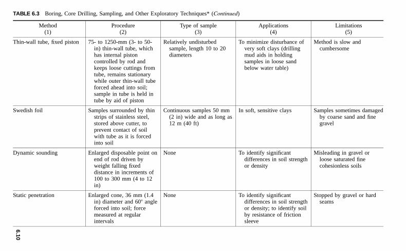
Thin-wall tube, ASTM D1587
75- to 1250-mm (3–50 in)thin-wall tube forced intosoil with static force (ordriven in soft rock);retention of sample helpedby drilling mud
Relatively undisturbedsample, length 10 to 20diameters
In soft to firm clays, short(5-diameter) samples ofstiff cohesive soil, softrock and, with aid ofdrilling mud, in firm todense sands
Cutting edge wrinkled bygravel; samples lost inloose sand or very softclay below water table;more disturbance occurs ifdriven with hammer
6.1
0
TABLE 6.3 Boring, Core Drilling, Sampling, and Other Exploratory Techniques* (Continued)
Method(1)
Procedure(2)
Type of sample(3)
Applications(4)
Limitations(5)
Thin-wall tube, fixed piston 75- to 1250-mm (3- to 50-in) thin-wall tube, whichhas internal pistoncontrolled by rod andkeeps loose cuttings fromtube, remains stationarywhile outer thin-wall tubeforced ahead into soil;sample in tube is held intube by aid of piston
Relatively undisturbedsample, length 10 to 20diameters
To minimize disturbance ofvery soft clays (drillingmud aids in holdingsamples in loose sandbelow water table)
Method is slow andcumbersome
Swedish foil Samples surrounded by thinstrips of stainless steel,stored above cutter, toprevent contact of soilwith tube as it is forcedinto soil
Continuous samples 50 mm(2 in) wide and as long as12 m (40 ft)
In soft, sensitive clays Samples sometimes damagedby coarse sand and finegravel
Dynamic sounding Enlarged disposable point onend of rod driven byweight falling fixeddistance in increments of100 to 300 mm (4 to 12in)
None To identify significantdifferences in soil strengthor density
Misleading in gravel orloose saturated finecohesionless soils
Static penetration Enlarged cone, 36 mm (1.4in) diameter and 60� angleforced into soil; forcemeasured at regularintervals
None To identify significantdifferences in soil strengthor density; to identify soilby resistance of frictionsleeve
Stopped by gravel or hardseams
6.1
1
TABLE 6.3 Boring, Core Drilling, Sampling, and Other Exploratory Techniques* (Continued)
Method(1)
Procedure(2)
Type of sample(3)
Applications(4)
Limitations(5)
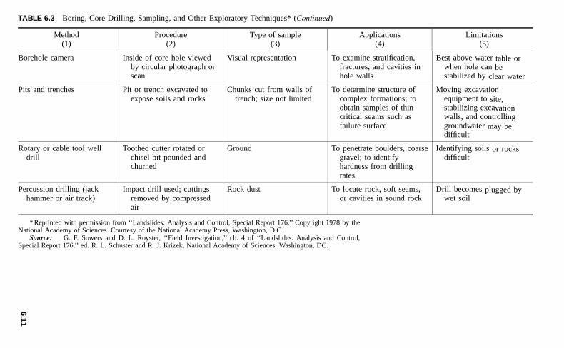
Borehole camera Inside of core hole viewedby circular photograph orscan
Visual representation To examine stratification,fractures, and cavities inhole walls
Best above water table orwhen hole can bestabilized by clear water
Pits and trenches Pit or trench excavated toexpose soils and rocks
Chunks cut from walls oftrench; size not limited
To determine structure ofcomplex formations; toobtain samples of thincritical seams such asfailure surface
Moving excavationequipment to site,stabilizing excavationwalls, and controllinggroundwater may bedifficult
Rotary or cable tool welldrill
Toothed cutter rotated orchisel bit pounded andchurned
Ground To penetrate boulders, coarsegravel; to identifyhardness from drillingrates
Identifying soils or rocksdifficult
Percussion drilling (jackhammer or air track)
Impact drill used; cuttingsremoved by compressedair
Rock dust To locate rock, soft seams,or cavities in sound rock
Drill becomes plugged bywet soil
* Reprinted with permission from ‘‘Landslides: Analysis and Control, Special Report 176,’’ Copyright 1978 by theNational Academy of Sciences. Courtesy of the National Academy Press, Washington, D.C.
Source: G. F. Sowers and D. L. Royster, ‘‘Field Investigation,’’ ch. 4 of ‘‘Landslides: Analysis and Control,Special Report 176,’’ ed. R. L. Schuster and R. J. Krizek, National Academy of Sciences, Washington, DC.
6.12 SECTION SIX
from the hole, and the soil lodged in the groves of the flight auger or containedin the bucket of the bucket auger is removed. A casing is generally not used forauger borings, and the hole may cave-in during the excavation of loose or softsoils or when the excavation is below the groundwater table. Augers are probablythe most common type of equipment used to excavate borings.Hollow-Stem Flight Auger. A hollow-stem flight auger has a circular hollowcore which allows for sampling down the center of the auger. The hollow-stemauger acts like a casing and allows for sampling in loose or soft soils or whenthe excavation is below the groundwater table.Wash-Type Borings. Wash-type borings use circulating drilling fluid, whichremoves cuttings from the borehole. The cuttings are created by the chopping,twisting, and jetting action of the drill bit, which breaks the soil or rock intosmall fragments. Casings are often used to prevent cave-in of the hole. Becausedrilling fluid is used during the excavation, it can be difficult to classify the soiland obtain uncontaminated soil samples.Rotary Coring. This type of boring equipment uses power rotation of the drill-ing bit as circulating fluid removes cuttings from the hole. Table 6.3 lists varioustypes of rotary coring for soil and rock.Percussion Drilling. This type of drilling equipment is often used to penetratehard rock, for subsurface exploration or for the purpose of drilling wells. Thedrill bit works much like a jackhammer, rising and falling to break up and crushthe rock material.
In addition to borings, other methods for performing subsurface exploration in-clude test pits and trenches. Test pits are often square in plan view, with a typicaldimension of 1.2 m by 1.2 m (4 ft by 4 ft). Trenches are long and narrow exca-vations usually made by a backhoe or bulldozer. Table 6.4 presents the uses, ca-pabilities, and limitations of test pits and trenches.
Test pits and trenches provide for a visual observation of subsurface conditions.They can also be used to obtain undisturbed block samples of soil. The processconsists of carving a block of soil from the side or bottom of the test pit or trench.Soil samples can also be obtained from the test pits or trenches by manually drivingShelby tubes, drive cylinders, or other types of sampling tubes into the ground.(See Art. 6.2.3.)
Backhoe trenches are an economical means of performing subsurface explora-tion. The backhoe can quickly excavate the trench, which can then be used toobserve and test the in-situ soil. In many subsurface explorations, backhoe trenchesare used to evaluate near-surface and geologic conditions (i.e., up to 15 ft deep),with borings being used to investigate deeper subsurface conditions.
6.2.3 Soil Sampling
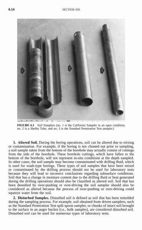
Many different types of samplers are used to retrieve soil and rock specimens fromthe borings. Common examples are indicated in Table 6.3. Figure 6.1 shows threetypes of samplers, the ‘‘California Sampler,’’ Shelby tube sampler, and StandardPenetration Test (SPT) sampler.
The most common type of soil sampler used in the United States is the Shelbytube, which is a thin-walled sampling tube. It can be manufactured to differentdiameters and lengths, with a typical diameter varying from 5 to 7.6 cm (2 to 3 in)and a length of 0.6 to 0.9 m (2 to 3 ft). The Shelby tube should be manufactured
SOIL MECHANICS AND FOUNDATIONS 6.13
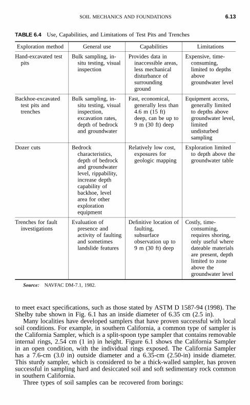
TABLE 6.4 Use, Capabilities, and Limitations of Test Pits and Trenches
Exploration method General use Capabilities Limitations
Hand-excavated testpits
Bulk sampling, in-situ testing, visualinspection
Provides data ininaccessible areas,less mechanicaldisturbance ofsurroundingground
Expensive, time-consuming,limited to depthsabovegroundwater level
Backhoe-excavatedtest pits andtrenches
Bulk sampling, in-situ testing, visualinspection,excavation rates,depth of bedrockand groundwater
Fast, economical,generally less than4.6 m (15 ft)deep, can be up to9 m (30 ft) deep
Equipment access,generally limitedto depths abovegroundwater level,limitedundisturbedsampling
Dozer cuts Bedrockcharacteristics,depth of bedrockand groundwaterlevel, rippability,increase depthcapability ofbackhoe, levelarea for otherexplorationequipment
Relatively low cost,exposures forgeologic mapping
Exploration limitedto depth above thegroundwater table
Trenches for faultinvestigations
Evaluation ofpresence andactivity of faultingand sometimeslandslide features
Definitive location offaulting,subsurfaceobservation up to9 m (30 ft) deep
Costly, time-consuming,requires shoring,only useful wheredateable materialsare present, depthlimited to zoneabove thegroundwater level
Source: NAVFAC DM-7.1, 1982.
to meet exact specifications, such as those stated by ASTM D 1587-94 (1998). TheShelby tube shown in Fig. 6.1 has an inside diameter of 6.35 cm (2.5 in).
Many localities have developed samplers that have proven successful with localsoil conditions. For example, in southern California, a common type of sampler isthe California Sampler, which is a split-spoon type sampler that contains removableinternal rings, 2.54 cm (1 in) in height. Figure 6.1 shows the California Samplerin an open condition, with the individual rings exposed. The California Samplerhas a 7.6-cm (3.0 in) outside diameter and a 6.35-cm (2.50-in) inside diameter.This sturdy sampler, which is considered to be a thick-walled sampler, has provensuccessful in sampling hard and desiccated soil and soft sedimentary rock commonin southern California.
Three types of soil samples can be recovered from borings:
6.14 SECTION SIX
FIGURE 6.1 Soil Samplers (no. 1 is the California Sampler in an open condition,no. 2 is a Shelby Tube, and no. 3 is the Standard Penetration Test sampler.)
1. Altered Soil. During the boring operations, soil can be altered due to mixingor contamination. For example, if the boring is not cleaned out prior to sampling,a soil sample taken from the bottom of the borehole may actually consist of cuttingsfrom the side of the borehole. These borehole cuttings, which have fallen to thebottom of the borehole, will not represent in-situ conditions at the depth sampled.In other cases, the soil sample may become contaminated with drilling fluid, whichis used for wash-type borings. These types of soil samples that have been mixedor contaminated by the drilling process should not be used for laboratory testsbecause they will lead to incorrect conclusions regarding subsurface conditions.Soil that has a change in moisture content due to the drilling fluid or heat generatedduring the drilling operations should also be classified as altered soil. Soil that hasbeen densified by over-pushing or over-driving the soil sampler should also beconsidered as altered because the process of over-pushing or over-driving couldsqueeze water from the soil.
2. Disturbed Samples. Disturbed soil is defined as soil that has been remoldedduring the sampling process. For example, soil obtained from driven samplers, suchas the Standard Penetration Test spilt spoon sampler, or chunks of intact soil broughtto the surface in an auger bucket (i.e., bulk samples), are considered disturbed soil.Disturbed soil can be used for numerous types of laboratory tests.
SOIL MECHANICS AND FOUNDATIONS 6.15
3. Undisturbed Sample. It should be recognized that no soil sample can betaken from the ground in a perfectly undisturbed state. However, this terminologyhas been applied to those soil samples taken by certain sampling methods. Undis-turbed samples are often defined as those samples obtained by slowly pushing thin-walled tubes, having sharp cutting ends and tip relief, into the soil. Two parameters,the inside clearance ratio and the area ratio, are often used to evaluate the dis-turbance potential of different samplers, and they are defined as follows:
D � Di einside clearance ratio (%) � 100 (6.1)De
2 2D � Do iarea ratio (%) � 100 (6.2)2Di
where De � diameter at the sampler cutting tipDi � inside diameter of the sampling tubeDo � outside diameter of the sampling tube
In general, a sampling tube for undisturbed soil specimens should have an insideclearance ratio of about 1% and an area ratio of about 10% or less. Having aninside clearance ratio of about 1% provides for tip relief of the soil and reducesthe friction between the soil and inside of the sampling tube during the samplingprocess. A thin film of oil can be applied at the cutting edge to also reduce thefriction between the soil and metal tube during sampling operations. The purposeof having a low area ratio and a sharp cutting end is to slice into the soil with aslittle disruption and displacement of the soil as possible. Shelby tubes are manu-factured to meet these specifications and are considered to be undisturbed soilsamplers. As a comparison, the California Sampler has an area ratio of 44% andis considered to be a thick-walled sampler.
It should be mentioned that using a thin-walled tube, such as a Shelby tube, willnot guarantee an undisturbed soil specimen. Many other factors can cause soildisturbance, such as:
• Pieces of hard gravel or shell fragments in the soil, which can cause voids todevelop along the sides of the sampling tube during the sampling process
• Soil adjustment caused by stress relief when making a borehole
• Disruption of the soil structure due to hammering or pushing the sampling tubeinto the soil stratum
• Expansion of gas during retrieval of the sampling tube
• Jarring or banging the sampling tube during transportation to the laboratory
• Roughly removing the soil from the sampling tube
• Crudely cutting the soil specimen to a specific size for a laboratory test
The actions listed above cause a decrease in effective stress, a reduction in theinterparticle bonds, and a rearrangement of the soil particles. An ‘‘undisturbed’’ soilspecimen will have little rearrangement of the soil particles and perhaps no distur-bance except that caused by stress relief where there is a change from the in-situstress condition to an isotropic ‘‘perfect sample’’ stress condition. A disturbed soilspecimen will have a disrupted soil structure with perhaps a total rearrangement of
6.16 SECTION SIX
soil particles. When measuring the shear strength or deformation characteristics ofthe soil, the results of laboratory tests run on undisturbed specimens obviouslybetter represent in-situ properties than laboratory tests run on disturbed specimens.
Soil samples recovered from the borehole should be kept within the samplingtube or sampling rings. The soil sampling tube should be tightly sealed with endcaps or the sampling rings thoroughly sealed in containers to prevent a loss ofmoisture during transportation to the laboratory. The soil samples should be markedwith the file or project number, date of sampling, name of engineer or geologistwho performed the sampling, and boring number and depth.
6.2.4 Field Testing
There are many different types of tests that can be performed at the time of drilling.The three most common types of field tests are discussed in this section:
Standard Penetration Test (SPT ). The Standard Penetration Test (SPT) consistsof driving a thick-walled sampler into a sand deposit. The SPT sampler must havean inside barrel diameter (Di) � 3.81 cm (1.5 in) and an outside diameter (Do) �5.08 cm (2 in). The SPT sampler is shown in Fig. 6.1. The SPT sampler is driveninto the sand by using a 63.5-kg (140-lb.) hammer falling a distance of 0.76 m (30in). The SPT sampler is driven a total of 45 cm (18 in), with the number of blowsrecorded for each 15 cm (6 in) interval. The ‘‘measured SPT N value’’ (blows perft) is defined as the penetration resistance of the sand, which equals the sum of thenumber of blows required to drive the SPT sampler over the depth interval of 15to 45 cm (6 to 18 in). The reason the number of blows required to drive the SPTsampler for the first 15 cm (6 in) is not included in the N value is that the drillingprocess often disturbs the soil at the bottom of the borehole and the readings at 15to 45 cm (6 to 18 in) are believed to be more representative of the in-situ penetrationresistance of the sand. The data below present a correlation between the measuredSPT N value (blows per ft) and the density condition of a clean sand deposit.
N value (blows per ft) Sand density Relative density
0 to 4 Very loose condition 0 to 15%4 to 10 Loose condition 15 to 35%
10 to 30 Medium condition 35 to 65%30 to 50 Dense condition 65 to 85%Over 50 Very dense condition 85 to 100%
Relative density is defined in Art. 6.3.4. Note that the above correlation is veryapproximate and the boundaries between different density conditions are not asdistinct as implied by the table.
The measured SPT N value can be influenced by many testing factors and soilconditions. For example, gravel-size particles increase the driving resistance (henceincreased N value) by becoming stuck in the SPT sampler tip or barrel. Anotherfactor that could influence the measured SPT N value is groundwater. It is importantto maintain a level of water in the borehole at or above the in-situ groundwaterlevel. This is to prevent groundwater from rushing into the bottom of the borehole,which could loosen the sand and result in low measured N values.
SOIL MECHANICS AND FOUNDATIONS 6.17
Besides gravel and groundwater conditions described above, there are manydifferent testing factors that can influence the accuracy of the SPT readings. Forexample, the measured SPT N value could be influenced by the hammer efficiency,rate at which the blows are applied, borehole diameter, and rod lengths. The fol-lowing equation is used to compensate for these testing factors (A. W. Skempton,‘‘Standard Penetration Test Procedures,’’ Geotechnique 36):
N � 1.67 E C C N (6.3)60 m b r
where N60 � SPT N value corrected for field testing procedures.Em � hammer efficiency (for U.S. equipment, Em equals 0.6 for a safety
hammer and Em equals 0.45 for a donut hammer)Cb � borehole diameter correction (Cb � 1.0 for boreholes of 65 to 115
mm (2.5 to 4.5 in) diameter, 1.05 for 150-mm diameter (5.9-in), and1.15 for 200-mm (7.9-in) diameter hole)
Cr � Rod length correction (Cr � 0.75 for up to 4 m (13 ft) of drill rods,0.85 for 4 to 6 m (13 to 20 ft) of drill rods, 0.95 for 6 to 10 m (20to 33 ft) of drill rods, and 1.00 for drill rods in excess of 10 m (33ft)
N � measured SPT N value
Even with the limitations and all of the corrections that must be applied to themeasured SPT N value, the Standard Penetration Test is probably the most widelyused field test in the United States. This is because it is relatively easy to use, thetest is economical as compared to other types of field testing, and the SPT equip-ment can be quickly adapted and included as part of almost any type of drillingrig.
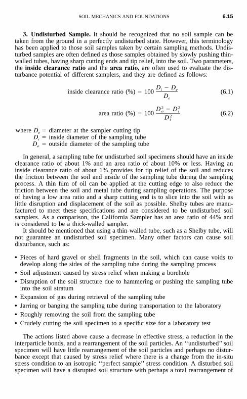
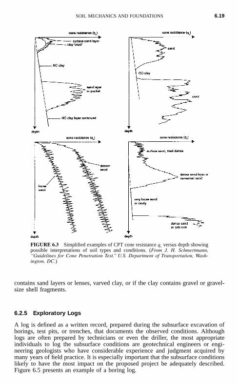
Cone Penetration Test (CPT ). The idea for the Cone Penetration Test (CPT) issimilar to that for the Standard Penetration Test, except that instead of a thick-walled sampler being driven into the soil, a steel cone is pushed into the soil. Thereare many different types of cone penetration devices, such as the mechanical cone,mechanical-friction cone, electric cone, and piezocone. The simplest type of coneis shown in Fig. 6.2. The cone is first pushed into the soil to the desired depth(initial position) and then a force is applied to the inner rods that moves the conedownward into the extended position. The force required to move the cone into theextended position (Fig. 6.2) divided by the horizontally projected area of the coneis defined as the cone resistance (qc). By continual repetition of the two-step processshown in Fig. 6.2, the cone resistance data is obtained at increments of depth. Acontinuous record of the cone resistance versus depth can be obtained by using theelectric cone, where the cone is pushed into the soil at a rate of 10 to 20 mm/sec(2 to 4 ft /min). Figure 6.3 presents four simplified examples of cone resistance(qc) versus depth profiles and the possible interpretation of the soil types and con-ditions.
A major advantage of the Cone Penetration Test is that by use of the electriccone, a continuous subsurface record of the cone resistance (qc) can be obtained.This is in contrast to the Standard Penetration Test, which obtains data at intervalsin the soil deposit. Disadvantages of the Cone Penetration Test are that soil samplescan not be recovered and special equipment is required to produce a steady andslow penetration of the cone. Unlike the SPT, the ability to obtain a steady andslow penetration of the cone is not included as part of conventional drilling rigs.Because of these factors, in the United States the CPT is used less frequently thanthe SPT.
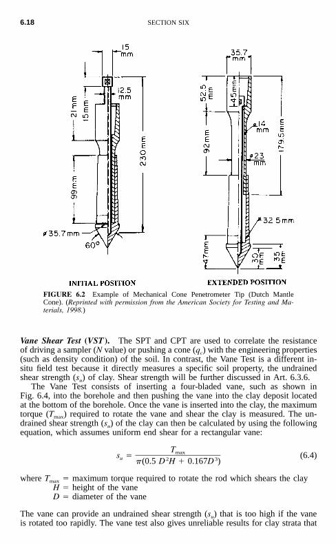
6.18 SECTION SIX
FIGURE 6.2 Example of Mechanical Cone Penetrometer Tip (Dutch MantleCone). (Reprinted with permission from the American Society for Testing and Ma-terials, 1998.)
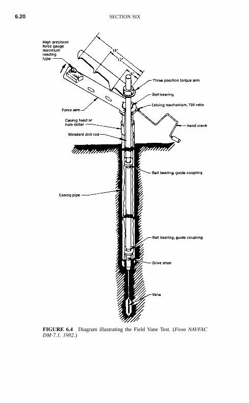
Vane Shear Test (VST ). The SPT and CPT are used to correlate the resistanceof driving a sampler (N value) or pushing a cone (qc) with the engineering properties(such as density condition) of the soil. In contrast, the Vane Test is a different in-situ field test because it directly measures a specific soil property, the undrainedshear strength (su) of clay. Shear strength will be further discussed in Art. 6.3.6.
The Vane Test consists of inserting a four-bladed vane, such as shown inFig. 6.4, into the borehole and then pushing the vane into the clay deposit locatedat the bottom of the borehole. Once the vane is inserted into the clay, the maximumtorque (Tmax) required to rotate the vane and shear the clay is measured. The un-drained shear strength (su) of the clay can then be calculated by using the followingequation, which assumes uniform end shear for a rectangular vane:
Tmaxs � (6.4)u 2 3� (0.5 D H � 0.167D )
where Tmax � maximum torque required to rotate the rod which shears the clayH � height of the vaneD � diameter of the vane
The vane can provide an undrained shear strength (su) that is too high if the vaneis rotated too rapidly. The vane test also gives unreliable results for clay strata that
SOIL MECHANICS AND FOUNDATIONS 6.19
FIGURE 6.3 Simplified examples of CPT cone resistance qc versus depth showingpossible interpretations of soil types and conditions. (From J. H. Schmertmann,‘‘Guidelines for Cone Penetration Test.’’ U.S. Department of Transportation, Wash-ington, DC.)
contains sand layers or lenses, varved clay, or if the clay contains gravel or gravel-size shell fragments.
6.2.5 Exploratory Logs
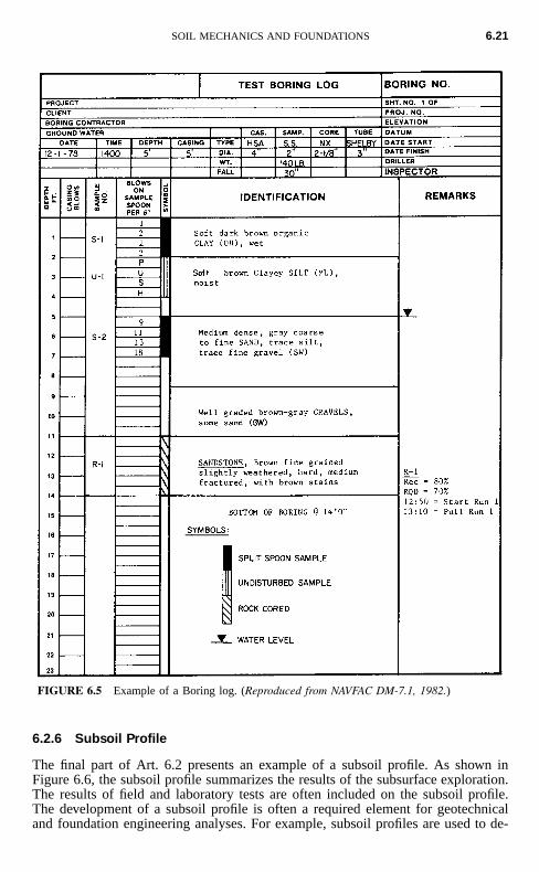
A log is defined as a written record, prepared during the subsurface excavation ofborings, test pits, or trenches, that documents the observed conditions. Althoughlogs are often prepared by technicians or even the driller, the most appropriateindividuals to log the subsurface conditions are geotechnical engineers or engi-neering geologists who have considerable experience and judgment acquired bymany years of field practice. It is especially important that the subsurface conditionslikely to have the most impact on the proposed project be adequately described.Figure 6.5 presents an example of a boring log.
6.20 SECTION SIX
FIGURE 6.4 Diagram illustrating the Field Vane Test. (From NAVFACDM-7.1, 1982.)
SOIL MECHANICS AND FOUNDATIONS 6.21
FIGURE 6.5 Example of a Boring log. (Reproduced from NAVFAC DM-7.1, 1982.)
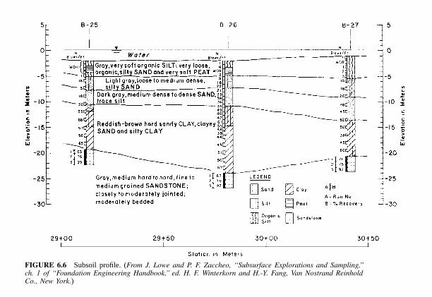
6.2.6 Subsoil Profile
The final part of Art. 6.2 presents an example of a subsoil profile. As shown inFigure 6.6, the subsoil profile summarizes the results of the subsurface exploration.The results of field and laboratory tests are often included on the subsoil profile.The development of a subsoil profile is often a required element for geotechnicaland foundation engineering analyses. For example, subsoil profiles are used to de-
6.2
2
FIGURE 6.6 Subsoil profile. (From J. Lowe and P. F. Zaccheo, ‘‘Subsurface Explorations and Sampling,’’ch. 1 of ‘‘Foundation Engineering Handbook,’’ ed. H. F. Winterkorn and H.-Y. Fang, Van Nostrand ReinholdCo., New York.)
SOIL MECHANICS AND FOUNDATIONS 6.23
termine the foundation type (shallow versus deep foundation), calculate the amountof settlement of the structure, evaluate the effect of groundwater on the project anddevelop recommendations for dewatering of underground structures, perform slopestability analyses for projects having sloping topography, and prepare site devel-opment recommendations.
6.3 LABORATORY TESTING
6.3.1 Introduction
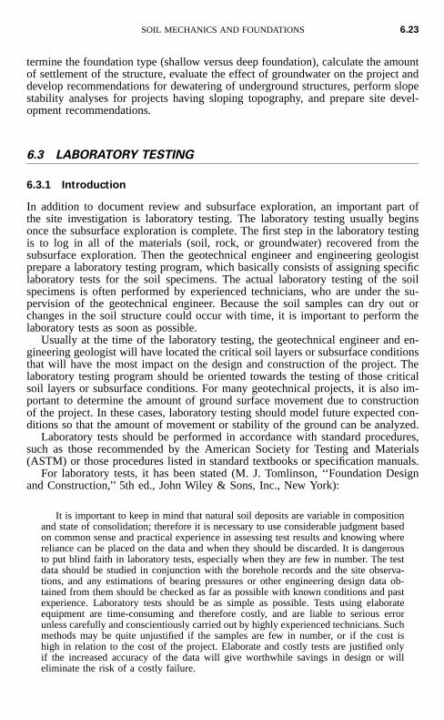
In addition to document review and subsurface exploration, an important part ofthe site investigation is laboratory testing. The laboratory testing usually beginsonce the subsurface exploration is complete. The first step in the laboratory testingis to log in all of the materials (soil, rock, or groundwater) recovered from thesubsurface exploration. Then the geotechnical engineer and engineering geologistprepare a laboratory testing program, which basically consists of assigning specificlaboratory tests for the soil specimens. The actual laboratory testing of the soilspecimens is often performed by experienced technicians, who are under the su-pervision of the geotechnical engineer. Because the soil samples can dry out orchanges in the soil structure could occur with time, it is important to perform thelaboratory tests as soon as possible.
Usually at the time of the laboratory testing, the geotechnical engineer and en-gineering geologist will have located the critical soil layers or subsurface conditionsthat will have the most impact on the design and construction of the project. Thelaboratory testing program should be oriented towards the testing of those criticalsoil layers or subsurface conditions. For many geotechnical projects, it is also im-portant to determine the amount of ground surface movement due to constructionof the project. In these cases, laboratory testing should model future expected con-ditions so that the amount of movement or stability of the ground can be analyzed.
Laboratory tests should be performed in accordance with standard procedures,such as those recommended by the American Society for Testing and Materials(ASTM) or those procedures listed in standard textbooks or specification manuals.
For laboratory tests, it has been stated (M. J. Tomlinson, ‘‘Foundation Designand Construction,’’ 5th ed., John Wiley & Sons, Inc., New York):
It is important to keep in mind that natural soil deposits are variable in compositionand state of consolidation; therefore it is necessary to use considerable judgment basedon common sense and practical experience in assessing test results and knowing wherereliance can be placed on the data and when they should be discarded. It is dangerousto put blind faith in laboratory tests, especially when they are few in number. The testdata should be studied in conjunction with the borehole records and the site observa-tions, and any estimations of bearing pressures or other engineering design data ob-tained from them should be checked as far as possible with known conditions and pastexperience. Laboratory tests should be as simple as possible. Tests using elaborateequipment are time-consuming and therefore costly, and are liable to serious errorunless carefully and conscientiously carried out by highly experienced technicians. Suchmethods may be quite unjustified if the samples are few in number, or if the cost ishigh in relation to the cost of the project. Elaborate and costly tests are justified onlyif the increased accuracy of the data will give worthwhile savings in design or willeliminate the risk of a costly failure.
6.24 SECTION SIX
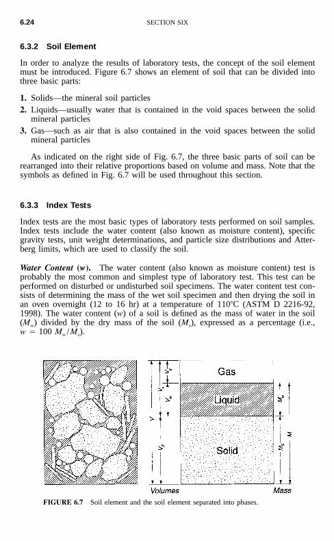
FIGURE 6.7 Soil element and the soil element separated into phases.
6.3.2 Soil Element
In order to analyze the results of laboratory tests, the concept of the soil elementmust be introduced. Figure 6.7 shows an element of soil that can be divided intothree basic parts:
1. Solids—the mineral soil particles2. Liquids—usually water that is contained in the void spaces between the solid
mineral particles3. Gas—such as air that is also contained in the void spaces between the solid
mineral particles
As indicated on the right side of Fig. 6.7, the three basic parts of soil can berearranged into their relative proportions based on volume and mass. Note that thesymbols as defined in Fig. 6.7 will be used throughout this section.
6.3.3 Index Tests
Index tests are the most basic types of laboratory tests performed on soil samples.Index tests include the water content (also known as moisture content), specificgravity tests, unit weight determinations, and particle size distributions and Atter-berg limits, which are used to classify the soil.
Water Content (w). The water content (also known as moisture content) test isprobably the most common and simplest type of laboratory test. This test can beperformed on disturbed or undisturbed soil specimens. The water content test con-sists of determining the mass of the wet soil specimen and then drying the soil inan oven overnight (12 to 16 hr) at a temperature of 110�C (ASTM D 2216-92,1998). The water content (w) of a soil is defined as the mass of water in the soil(Mw) divided by the dry mass of the soil (Ms), expressed as a percentage (i.e.,w � 100 Mw /Ms).
SOIL MECHANICS AND FOUNDATIONS 6.25
TABLE 6.5 Formula and Specific Gravity of Common Soil Minerals
Type of mineral FormulaSpecificgravity Comments
Quartz SiO2 2.65 Silicate, most common type of soilmineral
K FeldsparNa or Ca Feldspar
KAlSi3O8
NaAlSi3O8
2.54–2.572.62–2.76
Feldspars are also silicates and arethe second most common type ofsoil mineral.
Calcite CaCO3 2.71 Basic constituent of carbonate rocksDolomite CaMg(CO3)2 2.85 Basic constituent of carbonate rocksMuscovite varies 2.76–3.0 Silicate sheet type mineral (mica
group)Biotite complex 2.8–3.2 Silicate sheet type mineral (mica
group)Hematite Fe2O3 5.2–5.3 Frequent cause of reddish-brown
color in soilGypsum CaSO4�2H2O 2.35 Can lead to sulfate attack of concreteSerpentine Mg3Si2O5(OH)4 2.5–2.6 Silicate sheet or fibrous type mineralKaolinite Al2Si2O5(OH)4 2.61–2.66 Silicate clay mineral, low activityIllite complex 2.60–2.86 Silicate clay mineral, intermediate
activityMontmorillonite complex 2.74–2.78 Silicate clay mineral, highest activity
NOTE: Silicates are very common and account for about 80% of the minerals at the Earth’s surface.
Values of water content (w) can vary from essentially 0% up to 1200%. A watercontent of 0% indicates a dry soil. An example of a dry soil would be near-surfacerubble, gravel, or clean sand located in a hot and dry climate, such as Death Valley,California. Soil having the highest water content is organic soil, such as fibrouspeat, which has been reported to have a water content as high as 1200%.
Specific Gravity of Soil Solids (G). The specific gravity (G) is a dimensionlessparameter that is defined as the density of solids (�s) divided by the density ofwater (�w), or G � �s /�w. The density of solids (�s) is defined as the mass of solids(Ms) divided by the volume of solids (Vs). The density of water (�w) is equal to1 g/cm3 (or 1 Mg/m3) and 62.4 pcf.
For soil, the specific gravity is obtained by measuring the dry mass of the soiland then using a pycnometer to obtain the volume of the soil. Table 6.5 presentstypical values and ranges of specific gravity versus different types of soil minerals.Because quartz is the most abundant type of soil mineral, the specific gravity forinorganic soil is often assumed to be 2.65. For clays, the specific gravity is oftenassumed to be 2.70 because common clay particles, such as montmorillonite andillite, have slightly higher specific gravity values.
Total Unit Weight (�t ). The total unit weight (also known as the wet unit weight)should only be obtained from undisturbed soil specimens, such as those extrudedfrom Shelby tubes or on undisturbed block samples obtained from test pits andtrenches. The first step in the laboratory testing is to determine the wet density,defined as �t � M /V, where M � total mass of the soil, which is the sum of themass of water (Mw) and mass of solids (Ms), and V � total volume of the soil

6.26 SECTION SIX
TABLE 6.6 Unit Weight Relationships*
Parameter Relationships
Total unit weight (�t)W � W G� (1 � w)s w w� � �t V 1 � e
Dry unit weight (�d )W G� �s w t� � � �d V 1 � e 1 � w
Saturated unit weight (�sat)W � V � (G � e)� G� (1 � w)s v w w w� � � �sat V 1 � e 1 � G w
Note: The total unit weight (�t) is equal to the saturated unitweight (�sat) when all the void spaces are filled withwater (i.e., S � 100%).
Buoyant unit weight (�b)
� � � � �b sat w
� (G � 1) � (G � 1)w w� � �b 1 � e 1 � G wNote: The buoyant unit weight is also known as the
submerged unit weight.
* See Fig. 6.7 for definition of terms.Notes:1. For the equations listed in this table, water content (w) and degree of saturation (S ) must be
expressed as a decimal (not as a percentage).2. �w � density of water (1.0 Mg / m3, 62.4 pcf) and �w � unit weight of water (9.81 kN / m3, 62.4 pcf).
sample as defined in Fig. 6.7. The volume (V ) is determined by trimming the soilspecimen to a specific size or extruding the soil specimen directly from the samplerinto confining rings of known volume, and then the total mass (M) of the soilspecimen is obtained by using a balance.
The next step is to convert the wet density (�t) to total unit weight (�t). In orderto convert wet density to total unit weight in the International System of Units (SI),the wet density is multiplied by g (where g � acceleration of gravity � 9.81 m/sec2) to obtain the total unit weight, which has units of kN/m3. For example, inthe International System of Units, the density of water (�w) � 1.0 g/cm3 or 1.0Mg/m3, while the unit weight of water (�w) � 9.81 kN/m3.
In the United States Customary System, density and unit weight have exactlythe same value. Thus, the density of water and the unit weight of water are 62.4pcf. However, for the density of water (�w), the units should be thought of as lb-mass (lbm) per cubic ft, while for unit weight (�w), the units are lb-force (lbf) percubic foot. In the United States Customary System, it is common to assume that1 lbm � 1 lbf.
Typical values for total unit weight (�t) are 110 to 130 pcf (17 to 20 kN/m3).Besides the total unit weight, other types of unit weight are used in geotechnicalengineering. For example, the dry unit weight (�d ) refers to only the dry soil pervolume, while the saturated unit weight (�sat) refers to a special case where all thesoil voids are filled with water (i.e., saturated soil). Another commonly used unitweight is the buoyant unit weight (�b) which is used for calculations involving soillocated below the groundwater table. Table 6.6 presents various equations used to
SOIL MECHANICS AND FOUNDATIONS 6.27
calculate the different types of unit weights. Note in Table 6.6 that w � watercontent and G � specific gravity of soil solids. The void ratio (e) and degree ofsaturation (S) are discussed in the next article.
6.3.4 Phase Relationships
Phase relationships are the basic soil relationships used in geotechnical engineering.They are also known as weight-volume relationships. Different types of phase re-lationships are discussed below:
Void Ratio (e) and Porosity (n). The void ratio (e) is defined as the volume ofvoids (Vv) divided by the volume of solids (Vs). The porosity (n) is defined asvolume of voids (Vv) divided by the total volume (V). As indicated in Fig. 6.7, thevolume of voids is defined as the sum of the volume of air and volume of waterin the soil.
The void ratio (e) and porosity (n) are related as follows:
n ee � and n � (6.5)
1 � n 1 � e
The void ratio and porosity indicate the relative amount of void space in a soil.The lower the void ratio and porosity, the denser the soil (and vice versa). Thenatural soil having the lowest void ratio is probably till. For example, a typicalvalue of dry density for till is 2.34 Mg/m3 (146 pcf), which corresponds to a voidratio of 0.14. A typical till consists of a well-graded soil ranging in particle sizesfrom clay to gravel and boulders. The high density and low void ratio are due tothe extremely high stress exerted by glaciers. For compacted soil, the soil type withtypically the lowest void ratio is a well-graded decomposed granite (DG). A typicalvalue of maximum dry density (Modified Proctor) for a well-graded DG is 2.20Mg/m3 (137 pcf), which corresponds to a void ratio of 0.21. In general, the factorsneeded for a very low void ratio for compacted and naturally deposited soil are asfollows:
1. A well-graded grain-size distribution2. A high ratio of D100 /D0 (ratio of the largest and smallest grain sizes)3. Clay particles (having low activity) to fill in the smallest void spaces4. A process, such as compaction or the weight of glaciers, to compress the soil
particles into dense arrangements
At the other extreme are clays, such as sodium montmorillonite, which at lowconfining pressures can have a void ratio of more than 25. Highly organic soil,such as peat, can have even higher void ratios.
Degree of Saturation (S). The degree of saturation (S) is defined as:
100 VwS(%) � (6.6)Vv
The degree of saturation indicates the degree to which the soil voids are filled
6.28 SECTION SIX
with water. A totally dry soil will have a degree of saturation of 0%, while asaturated soil, such as a soil below the groundwater table, will have a degree ofsaturation of 100%. Typical ranges of degree of saturation versus soil condition areas follows:
Dry: S � 0%Humid: S � 1 to 25%Damp: S � 26 to 50%Moist: S � 51 to 75%Wet: S � 76 to 99%Saturated: S � 100%
Relative Density. The relative density is a measure of the density state of a non-plastic soil. The relative density can only be used for soil that is nonplastic, suchas sands and gravels. The relative density (Dr in %) is defined as:
e � emaxD (%) � 100 (6.7)r e � emax min
where emax � void ratio corresponding to the loosest possible state of the soil, usu-ally obtained by pouring the soil into a mold of known volume
emin � void ratio corresponding to the densest possible state of the soil,usually obtained by vibrating the soil particles into a dense state
e � the natural void ratio of the soil
The density state of the natural soil can be described as follows:
Very loose condition Dr � 0 to 15%Loose condition Dr � 15 to 35%Medium condition Dr � 35 to 65%Dense condition Dr � 65 to 85%Very dense condition Dr � 85 to 100%
The relative density (Dr) should not be confused with the relative compaction(RC), which will be discussed in Art. 6.10.1.
Useful Relationships. A frequently used method of solving phase relationships isfirst to fill in the phase diagram shown in Fig. 6.7. Once the different mass andvolumes are known, the various phase relationships can be determined. Anotherapproach is to use equations that relate different parameters. A useful relationshipis as follows:
Gw � Se (6.8)
where G � specific gravity of soil solidsw � water contentS � degree of saturatione � void ratio
Other commonly used relationships are presented in Table 6.7.
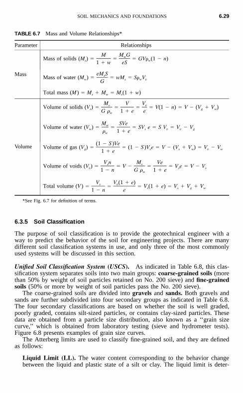
SOIL MECHANICS AND FOUNDATIONS 6.29
TABLE 6.7 Mass and Volume Relationships*
Parameter Relationships
Mass
M M GwMass of solids (M ) � � � GV� (1 � n)s w1 � w eS
eM SsMass of water (M ) � � wM � S� Vw s w vG
Total mass (M ) � M � M � M (1 � w)s w s
Volume
M V Vs vVolume of solids (V ) � � � � V(1 � n) � V � (V � V )s g wG � 1 � e ew
M SVewVolume of water (V ) � � � SV e � S V � V � Vw s v v g� 1 � ew
(1 � S )VeVolume of gas (V ) � � (1 � S )V e � V � (V � V ) � V � Vg s s w v w1 � e
V n M Ves sVolume of voids (V ) � � V � � � V e � V � Vv s s1 � n G � 1 � ew
V V (1 � e)s vTotal volume (V ) � � � V (1 � e) � V � V � Vs s g w1 � n e
*See Fig. 6.7 for definition of terms.
6.3.5 Soil Classification
The purpose of soil classification is to provide the geotechnical engineer with away to predict the behavior of the soil for engineering projects. There are manydifferent soil classification systems in use, and only three of the most commonlyused systems will be discussed in this section.
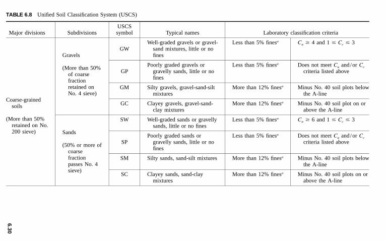
Unified Soil Classification System (USCS). As indicated in Table 6.8, this clas-sification system separates soils into two main groups: coarse-grained soils (morethan 50% by weight of soil particles retained on No. 200 sieve) and fine-grainedsoils (50% or more by weight of soil particles pass the No. 200 sieve).
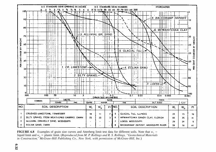
The coarse-grained soils are divided into gravels and sands. Both gravels andsands are further subdivided into four secondary groups as indicated in Table 6.8.The four secondary classifications are based on whether the soil is well graded,poorly graded, contains silt-sized particles, or contains clay-sized particles. Thesedata are obtained from a particle size distribution, also known as a ‘‘grain sizecurve,’’ which is obtained from laboratory testing (sieve and hydrometer tests).Figure 6.8 presents examples of grain size curves.
The Atterberg limits are used to classify fine-grained soil, and they are definedas follows:
Liquid Limit (LL). The water content corresponding to the behavior changebetween the liquid and plastic state of a silt or clay. The liquid limit is deter-
6.3
0
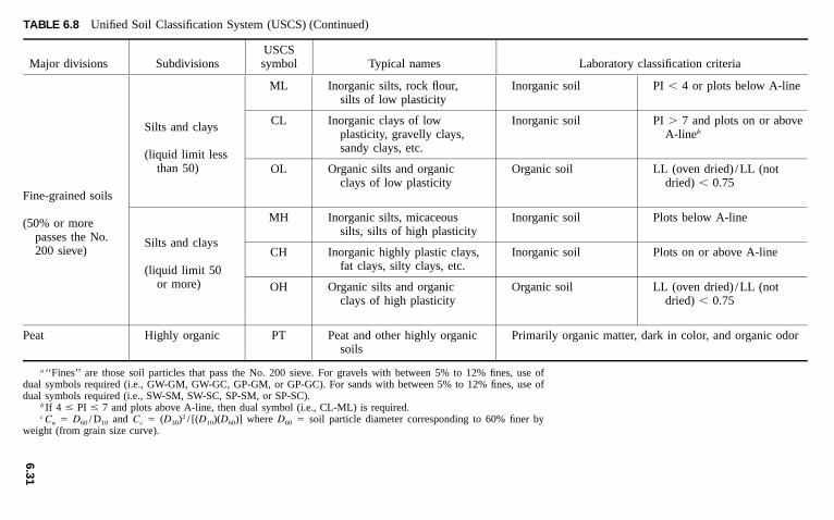
TABLE 6.8 Unified Soil Classification System (USCS)
Major divisions SubdivisionsUSCSsymbol Typical names Laboratory classification criteria
Coarse-grainedsoils
(More than 50%retained on No.200 sieve)
Gravels
(More than 50%of coarsefractionretained onNo. 4 sieve)
Sands
(50% or more ofcoarsefractionpasses No. 4sieve)
GW
GP
GM
GC
SW
SP
SM
SC
Well-graded gravels or gravel-sand mixtures, little or nofines
Poorly graded gravels orgravelly sands, little or nofines
Silty gravels, gravel-sand-siltmixtures
Clayey gravels, gravel-sand-clay mixtures
Well-graded sands or gravellysands, little or no fines
Poorly graded sands orgravelly sands, little or nofines
Silty sands, sand-silt mixtures
Clayey sands, sand-claymixtures
Less than 5% finesa
Less than 5% finesa
More than 12% finesa
More than 12% finesa
Less than 5% finesa
Less than 5% finesa
More than 12% finesa
More than 12% finesa
Cu � 4 and 1 � Cc � 3
Does not meet Cu and /or Cc
criteria listed above
Minus No. 40 soil plots belowthe A-line
Minus No. 40 soil plot on orabove the A-line
Cu � 6 and 1 � Cc � 3
Does not meet Cu and /or Cc
criteria listed above
Minus No. 40 soil plots belowthe A-line
Minus No. 40 soil plots on orabove the A-line
6.31
TABLE 6.8 Unified Soil Classification System (USCS) (Continued)
Major divisions SubdivisionsUSCSsymbol Typical names Laboratory classification criteria
Fine-grained soils
(50% or morepasses the No.200 sieve)
Silts and clays
(liquid limit lessthan 50)
Silts and clays
(liquid limit 50or more)
ML
CL
OL
MH
CH
OH
Inorganic silts, rock flour,silts of low plasticity
Inorganic clays of lowplasticity, gravelly clays,sandy clays, etc.
Organic silts and organicclays of low plasticity
Inorganic silts, micaceoussilts, silts of high plasticity
Inorganic highly plastic clays,fat clays, silty clays, etc.
Organic silts and organicclays of high plasticity
Inorganic soil
Inorganic soil
Organic soil
Inorganic soil
Inorganic soil
Organic soil
PI � 4 or plots below A-line
PI � 7 and plots on or aboveA-lineb
LL (oven dried) /LL (notdried) � 0.75
Plots below A-line
Plots on or above A-line
LL (oven dried) /LL (notdried) � 0.75
Peat Highly organic PT Peat and other highly organicsoils
Primarily organic matter, dark in color, and organic odor
a ‘‘Fines’’ are those soil particles that pass the No. 200 sieve. For gravels with between 5% to 12% fines, use ofdual symbols required (i.e., GW-GM, GW-GC, GP-GM, or GP-GC). For sands with between 5% to 12% fines, use ofdual symbols required (i.e., SW-SM, SW-SC, SP-SM, or SP-SC).
b If 4 � PI � 7 and plots above A-line, then dual symbol (i.e., CL-ML) is required.c Cu � D60 / D10 and Cc � (D30)2 / [(D10)(D60)] where D60 � soil particle diameter corresponding to 60% finer by
weight (from grain size curve).
6.3
2
FIGURE 6.8 Examples of grain size curves and Atterberg limit test data for different soils. Note that w1 �liquid limit and wp � plastic limit. (Reproduced from M. P. Rollings and R. S. Rollings, ‘‘Geotechnical Materialsin Construction,’’ McGraw-Hill Publishing Co., New York, with permission of McGraw-Hill, Inc.)
SOIL MECHANICS AND FOUNDATIONS 6.33
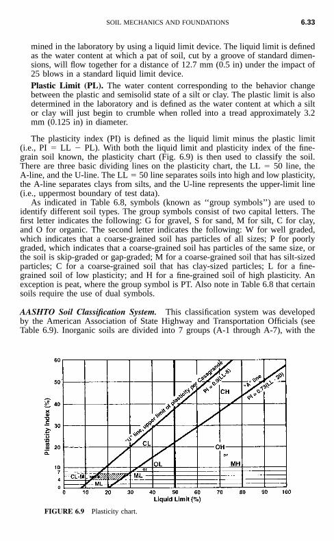
FIGURE 6.9 Plasticity chart.
mined in the laboratory by using a liquid limit device. The liquid limit is definedas the water content at which a pat of soil, cut by a groove of standard dimen-sions, will flow together for a distance of 12.7 mm (0.5 in) under the impact of25 blows in a standard liquid limit device.Plastic Limit (PL). The water content corresponding to the behavior changebetween the plastic and semisolid state of a silt or clay. The plastic limit is alsodetermined in the laboratory and is defined as the water content at which a siltor clay will just begin to crumble when rolled into a tread approximately 3.2mm (0.125 in) in diameter.
The plasticity index (PI) is defined as the liquid limit minus the plastic limit(i.e., PI � LL � PL). With both the liquid limit and plasticity index of the fine-grain soil known, the plasticity chart (Fig. 6.9) is then used to classify the soil.There are three basic dividing lines on the plasticity chart, the LL � 50 line, theA-line, and the U-line. The LL � 50 line separates soils into high and low plasticity,the A-line separates clays from silts, and the U-line represents the upper-limit line(i.e., uppermost boundary of test data).
As indicated in Table 6.8, symbols (known as ‘‘group symbols’’) are used toidentify different soil types. The group symbols consist of two capital letters. Thefirst letter indicates the following: G for gravel, S for sand, M for silt, C for clay,and O for organic. The second letter indicates the following: W for well graded,which indicates that a coarse-grained soil has particles of all sizes; P for poorlygraded, which indicates that a coarse-grained soil has particles of the same size, orthe soil is skip-graded or gap-graded; M for a coarse-grained soil that has silt-sizedparticles; C for a coarse-grained soil that has clay-sized particles; L for a fine-grained soil of low plasticity; and H for a fine-grained soil of high plasticity. Anexception is peat, where the group symbol is PT. Also note in Table 6.8 that certainsoils require the use of dual symbols.
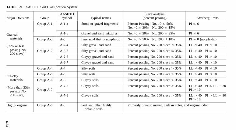
AASHTO Soil Classification System. This classification system was developedby the American Association of State Highway and Transportation Officials (seeTable 6.9). Inorganic soils are divided into 7 groups (A-1 through A-7), with the
6.3
4
TABLE 6.9 AASHTO Soil Classification System
Major Divisions GroupAASHTO
symbol Typical namesSieve analysis
(percent passing) Atterberg limits
Granualmaterials
(35% or lesspassing No.200 sieve)
Group A-1
Group A-3
Group A-2
A-1-a
A-1-b
A-3
A-2-4
A-2-5
A-2-6
A-2-7
Stone or gravel fragments
Gravel and sand mixtures
Fine sand that is nonplastic
Silty gravel and sand
Silty gravel and sand
Clayey gravel and sand
Clayey gravel and sand
Percent Passing: No. 10 � 50%No. 40 � 30% No. 200 � 15%
No. 40 � 50% No. 200 � 25%
No. 40 � 50% No. 200 � 10%
Percent passing No. 200 sieve � 35%
Percent passing No. 200 sieve � 35%
Percent passing No. 200 sieve � 35%
Percent passing No. 200 sieve � 35%
PI � 6
PI � 6
PI � 0 (nonplastic)
LL � 40 PI � 10
LL � 40 PI � 10
LL � 40 PI � 10
LL � 40 PI � 10
Silt-claymaterials
(More than 35%passing No.200 sieve)
Group A-4
Group A-5
Group A-6
Group A-7
A-4
A-5
A-6
A-7-5
A-7-6
Silty soils
Silty soils
Clayey soils
Clayey soils
Clayey soils
Percent passing No. 200 sieve � 35%
Percent passing No. 200 sieve � 35%
Percent passing No. 200 sieve � 35%
Percent passing No. 200 sieve � 35%
Percent passing No. 200 sieve � 35%
LL � 40 PI � 10
LL � 40 PI � 10
LL � 40 PI � 10
LL � 40 PI � LL � 30PI � 10
LL � 40 PI � LL � 30PI � 10
Highly organic Group A-8 A-8 Peat and other highlyorganic soils
Primarily organic matter, dark in color, and organic odor
6.3
5
Notes:1. Classification Procedure: First decide which of the three main categories (granular materials, silt-clay materials,
or highly organic) the soil belongs. Then proceed from the top to the bottom of the chart and the first group thatmeets the particle size and Atterberg limits criteria is the correct classification.
2. Group Index � (F � 35)[0.2 � 0.005(LL � 40)] � 0.01(F � 15)(PI � 10), where F � percent passing No.200 sieve, LL � liquid limit, and PI � plasticity index. Report group index to nearest whole number. For negativegroup index, report as zero. When working with A-2-6 and A-2-7 subgroups, use only the PI portion of thegroup index equation.
3. Atterberg limits are performed on soil passing the No. 40 sieve. LL � liquid limit, PL � plastic limit, andPI � plasticity index.
4. AASHTO definitions of particle sizes are as follows: (a) boulders: above 75 mm, (b) gravel: 75 mm to No. 10sieve, (c) coarse sand: No. 10 to No. 40 sieve, (d) fine sand: No. 40 to No. 200 sieve, and (e) silt-clay sizeparticles: material passing No. 200 sieve.
5. Example: An example of an AASHTO classification for a clay is A-7-6 (30), or Group A-7, subgroup 6, groupindex 30.
6.36 SECTION SIX
eighth group (A-8) reserved for highly organic soils. Soil types A-1, A-2, andA-7 have subgroups as indicated in Table 6.9. Those soils having plastic fines canbe further categorized by using the group index (defined in Table 6.9). GroupsA-1-a, A-1-b, A-3, A-2-4, and A-2-5 should be considered to have a group indexequal to zero. According to AASHTO, the road supporting characteristics of asubgrade may be assumed as an inverse ratio to its group index. Thus, a roadsubgrade having a group index of 0 indicates a ‘‘good’’ subgrade material that willoften provide good drainage and adequate bearing when thoroughly compacted. Aroad subgrade material that has a group index of 20 or greater indicates a ‘‘verypoor’’ subgrade material that will often be impervious and have a low bearingcapacity.
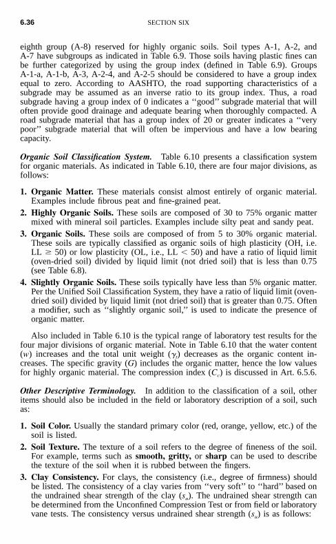
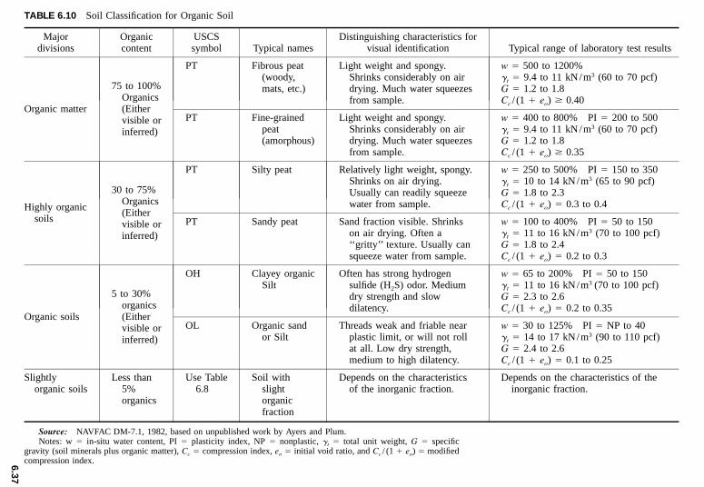
Organic Soil Classification System. Table 6.10 presents a classification systemfor organic materials. As indicated in Table 6.10, there are four major divisions, asfollows:
1. Organic Matter. These materials consist almost entirely of organic material.Examples include fibrous peat and fine-grained peat.
2. Highly Organic Soils. These soils are composed of 30 to 75% organic mattermixed with mineral soil particles. Examples include silty peat and sandy peat.
3. Organic Soils. These soils are composed of from 5 to 30% organic material.These soils are typically classified as organic soils of high plasticity (OH, i.e.LL � 50) or low plasticity (OL, i.e., LL � 50) and have a ratio of liquid limit(oven-dried soil) divided by liquid limit (not dried soil) that is less than 0.75(see Table 6.8).
4. Slightly Organic Soils. These soils typically have less than 5% organic matter.Per the Unified Soil Classification System, they have a ratio of liquid limit (oven-dried soil) divided by liquid limit (not dried soil) that is greater than 0.75. Oftena modifier, such as ‘‘slightly organic soil,’’ is used to indicate the presence oforganic matter.
Also included in Table 6.10 is the typical range of laboratory test results for thefour major divisions of organic material. Note in Table 6.10 that the water content(w) increases and the total unit weight (�t) decreases as the organic content in-creases. The specific gravity (G) includes the organic matter, hence the low valuesfor highly organic material. The compression index (Cc) is discussed in Art. 6.5.6.
Other Descriptive Terminology. In addition to the classification of a soil, otheritems should also be included in the field or laboratory description of a soil, suchas:
1. Soil Color. Usually the standard primary color (red, orange, yellow, etc.) of thesoil is listed.
2. Soil Texture. The texture of a soil refers to the degree of fineness of the soil.For example, terms such as smooth, gritty, or sharp can be used to describethe texture of the soil when it is rubbed between the fingers.
3. Clay Consistency. For clays, the consistency (i.e., degree of firmness) shouldbe listed. The consistency of a clay varies from ‘‘very soft’’ to ‘‘hard’’ based onthe undrained shear strength of the clay (su). The undrained shear strength canbe determined from the Unconfined Compression Test or from field or laboratoryvane tests. The consistency versus undrained shear strength (su) is as follows:
6.3
7
TABLE 6.10 Soil Classification for Organic Soil
Majordivisions
Organiccontent
USCSsymbol Typical names
Distinguishing characteristics forvisual identification Typical range of laboratory test results
Organic matter
75 to 100%Organics(Eithervisible orinferred)
PT
PT
Fibrous peat(woody,mats, etc.)
Fine-grainedpeat(amorphous)
Light weight and spongy.Shrinks considerably on airdrying. Much water squeezesfrom sample.
Light weight and spongy.Shrinks considerably on airdrying. Much water squeezesfrom sample.
w � 500 to 1200%�t � 9.4 to 11 kN/m3 (60 to 70 pcf)G � 1.2 to 1.8Cc / (1 � eo) � 0.40
w � 400 to 800% PI � 200 to 500�t � 9.4 to 11 kN/m3 (60 to 70 pcf)G � 1.2 to 1.8Cc / (1 � eo) � 0.35
Highly organicsoils
30 to 75%Organics(Eithervisible orinferred)
PT
PT
Silty peat
Sandy peat
Relatively light weight, spongy.Shrinks on air drying.Usually can readily squeezewater from sample.
Sand fraction visible. Shrinkson air drying. Often a‘‘gritty’’ texture. Usually cansqueeze water from sample.
w � 250 to 500% PI � 150 to 350�t � 10 to 14 kN/m3 (65 to 90 pcf)G � 1.8 to 2.3Cc / (1 � eo) � 0.3 to 0.4
w � 100 to 400% PI � 50 to 150�t � 11 to 16 kN/m3 (70 to 100 pcf)G � 1.8 to 2.4Cc / (1 � eo) � 0.2 to 0.3
Organic soils
5 to 30%organics(Eithervisible orinferred)
OH
OL
Clayey organicSilt
Organic sandor Silt
Often has strong hydrogensulfide (H2S) odor. Mediumdry strength and slowdilatency.
Threads weak and friable nearplastic limit, or will not rollat all. Low dry strength,medium to high dilatency.
w � 65 to 200% PI � 50 to 150�t � 11 to 16 kN/m3 (70 to 100 pcf)G � 2.3 to 2.6Cc / (1 � eo) � 0.2 to 0.35
w � 30 to 125% PI � NP to 40�t � 14 to 17 kN/m3 (90 to 110 pcf)G � 2.4 to 2.6Cc / (1 � eo) � 0.1 to 0.25
Slightlyorganic soils
Less than5%organics
Use Table6.8
Soil withslightorganicfraction
Depends on the characteristicsof the inorganic fraction.
Depends on the characteristics of theinorganic fraction.
Source: NAVFAC DM-7.1, 1982, based on unpublished work by Ayers and Plum.Notes: w � in-situ water content, PI � plasticity index, NP � nonplastic, �t � total unit weight, G � specific
gravity (soil minerals plus organic matter), Cc � compression index, eo � initial void ratio, and Cc / (1 � eo) � modifiedcompression index.
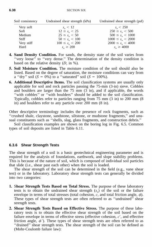
6.38 SECTION SIX
Soil consistency Undrained shear strength (kPa) Undrained shear strength (psf)
Very soft su � 12 su � 250Soft 12 � su � 25 250 � su � 500Medium 25 � su � 50 500 � su � 1000Stiff 50 � su � 100 1000 � su � 2000Very stiff 100 � su � 200 2000 � su � 4000Hard su � 200 su � 4000
4. Sand Density Condition. For sands, the density state of the soil varies from‘‘very loose’’ to ‘‘very dense.’’ The determination of the density condition isbased on the relative density (Dr in %).
5. Soil Moisture Condition. The moisture condition of the soil should also belisted. Based on the degree of saturation, the moisture conditions can vary froma ‘‘dry’’ soil (S � 0%) to a ‘‘saturated’’ soil (S � 100%).
6. Additional Descriptive Items. The soil classification systems are usually onlyapplicable for soil and rock particles passing the 75-mm (3-in) sieve. Cobblesand boulders are larger than the 75 mm (3 in), and if applicable, the words‘‘with cobbles’’ or ‘‘with boulders’’ should be added to the soil classification.Typically, cobbles refer to particles ranging from 75 mm (3 in) to 200 mm (8in) and boulders refer to any particle over 200 mm (8 in).
Other descriptive terminology includes the presence of rock fragments, such as‘‘crushed shale, claystone, sandstone, siltstone, or mudstone fragments,’’ and unu-sual constituents such as ‘‘shells, slag, glass fragments, and construction debris.’’
Soil classification examples are shown on the boring log in Fig. 6.5. Commontypes of soil deposits are listed in Table 6.11.
6.3.6 Shear Strength Tests
The shear strength of a soil is a basic geotechnical engineering parameter and isrequired for the analysis of foundations, earthwork, and slope stability problems.This is because of the nature of soil, which is composed of individual soil particlesthat slide (i.e., shear past each other) when the soil is loaded.
The shear strength of the soil can be determined in the field (e.g., vane sheartest) or in the laboratory. Laboratory shear strength tests can generally be dividedinto two categories:
1. Shear Strength Tests Based on Total Stress. The purpose of these laboratorytests is to obtain the undrained shear strength (su) of the soil or the failureenvelope in terms of total stresses (total cohesion, c, and total friction angle, �).These types of shear strength tests are often referred to as ‘‘undrained’’ shearstrength tests.
2. Shear Strength Tests Based on Effective Stress. The purpose of these labo-ratory tests is to obtain the effective shear strength of the soil based on thefailure envelope in terms of effective stress (effective cohesion, c�, and effectivefriction angle, ��). These types of shear strength tests are often referred to as‘‘drained’’ shear strength tests. The shear strength of the soil can be defined as(Mohr-Coulomb failure law):
SOIL MECHANICS AND FOUNDATIONS 6.39
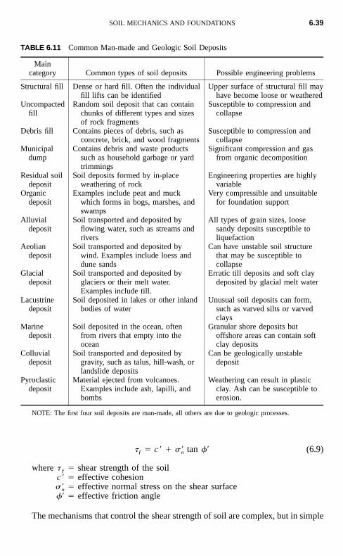
TABLE 6.11 Common Man-made and Geologic Soil Deposits
Maincategory Common types of soil deposits Possible engineering problems
Structural fill Dense or hard fill. Often the individualfill lifts can be identified
Upper surface of structural fill mayhave become loose or weathered
Uncompactedfill
Random soil deposit that can containchunks of different types and sizesof rock fragments
Susceptible to compression andcollapse
Debris fill Contains pieces of debris, such asconcrete, brick, and wood fragments
Susceptible to compression andcollapse
Municipaldump
Contains debris and waste productssuch as household garbage or yardtrimmings
Significant compression and gasfrom organic decomposition
Residual soildeposit
Soil deposits formed by in-placeweathering of rock
Engineering properties are highlyvariable
Organicdeposit
Examples include peat and muckwhich forms in bogs, marshes, andswamps
Very compressible and unsuitablefor foundation support
Alluvialdeposit
Soil transported and deposited byflowing water, such as streams andrivers
All types of grain sizes, loosesandy deposits susceptible toliquefaction
Aeoliandeposit
Soil transported and deposited bywind. Examples include loess anddune sands
Can have unstable soil structurethat may be susceptible tocollapse
Glacialdeposit
Soil transported and deposited byglaciers or their melt water.Examples include till.
Erratic till deposits and soft claydeposited by glacial melt water
Lacustrinedeposit
Soil deposited in lakes or other inlandbodies of water
Unusual soil deposits can form,such as varved silts or varvedclays
Marinedeposit
Soil deposited in the ocean, oftenfrom rivers that empty into theocean
Granular shore deposits butoffshore areas can contain softclay deposits
Colluvialdeposit
Soil transported and deposited bygravity, such as talus, hill-wash, orlandslide deposits
Can be geologically unstabledeposit
Pyroclasticdeposit
Material ejected from volcanoes.Examples include ash, lapilli, andbombs
Weathering can result in plasticclay. Ash can be susceptible toerosion.
NOTE: The first four soil deposits are man-made, all others are due to geologic processes.
� c � � � tan �� (6.9)ƒ n
where �ƒ shear strength of the soilc � � effective cohesion ��n effective normal stress on the shear surface�� � effective friction angle
The mechanisms that control the shear strength of soil are complex, but in simple
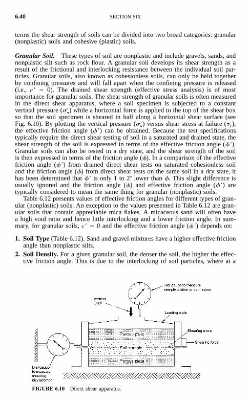
6.40 SECTION SIX
FIGURE 6.10 Direct shear apparatus.
terms the shear strength of soils can be divided into two broad categories: granular(nonplastic) soils and cohesive (plastic) soils.
Granular Soil. These types of soil are nonplastic and include gravels, sands, andnonplastic silt such as rock flour. A granular soil develops its shear strength as aresult of the frictional and interlocking resistance between the individual soil par-ticles. Granular soils, also known as cohesionless soils, can only be held togetherby confining pressures and will fall apart when the confining pressure is released(i.e., c � � 0). The drained shear strength (effective stress analysis) is of mostimportance for granular soils. The shear strength of granular soils is often measuredin the direct shear apparatus, where a soil specimen is subjected to a constantvertical pressure ( ) while a horizontal force is applied to the top of the shear box�nso that the soil specimen is sheared in half along a horizontal shear surface (seeFig. 6.10). By plotting the vertical pressure ( ) versus shear stress at failure (ƒ ),�nthe effective friction angle (��) can be obtained. Because the test specificationstypically require the direct shear testing of soil in a saturated and drained state, theshear strength of the soil is expressed in terms of the effective friction angle (��).Granular soils can also be tested in a dry state, and the shear strength of the soilis then expressed in terms of the friction angle (�). In a comparison of the effectivefriction angle (��) from drained direct shear tests on saturated cohesionless soiland the friction angle (�) from direct shear tests on the same soil in a dry state, ithas been determined that �� is only 1 to 2� lower than �. This slight difference isusually ignored and the friction angle (�) and effective friction angle (��) aretypically considered to mean the same thing for granular (nonplastic) soils.
Table 6.12 presents values of effective friction angles for different types of gran-ular (nonplastic) soils. An exception to the values presented in Table 6.12 are gran-ular soils that contain appreciable mica flakes. A micaceous sand will often havea high void ratio and hence little interlocking and a lower friction angle. In sum-mary, for granular soils, c � � 0 and the effective friction angle (��) depends on:
1. Soil Type (Table 6.12). Sand and gravel mixtures have a higher effective frictionangle than nonplastic silts.
2. Soil Density. For a given granular soil, the denser the soil, the higher the effec-tive friction angle. This is due to the interlocking of soil particles, where at a
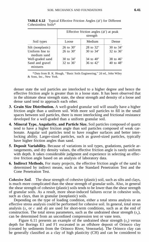
SOIL MECHANICS AND FOUNDATIONS 6.41
TABLE 6.12 Typical Effective Friction Angles (��) for DifferentCohesionless Soils*
Soil types
Effective friction angles (��) at peakstrength
Loose Medium Dense
Silt (nonplastic) 26 to 30� 28 to 32� 30 to 34�Uniform fine to
medium sand26 to 30� 30 to 34� 32 to 36�
Well-graded sand 30 to 34� 34 to 40� 38 to 46�Sand and gravel
mixtures32 to 36� 36 to 42� 40 to 48�
* Data from B. K. Hough, ‘‘Basic Soils Engineering,’’ 2d ed., John Wiley& Sons, Inc., New York.
denser state the soil particles are interlocked to a higher degree and hence theeffective friction angle is greater than in a loose state. It has been observed thatin the ultimate shear strength state, the shear strength and density of a loose anddense sand tend to approach each other.
3. Grain Size Distribution. A well-graded granular soil will usually have a higherfriction angle than a uniform soil. With more soil particles to fill in the smallspaces between soil particles, there is more interlocking and frictional resistancedeveloped for a well-graded than a uniform granular soil.
4. Mineral Type, Angularity, and Particle Size. Soil particles composed of quartztend to have a higher friction angle than soil particles composed of weak car-bonate. Angular soil particles tend to have rougher surfaces and better inter-locking ability. Larger-sized particles, such as gravel-sized particles, typicallyhave higher friction angles than sand.
5. Deposit Variability. Because of variations in soil types, gradations, particle ar-rangements, and dry density values, the effective friction angle is rarely uniformwith depth. It takes considerable judgment and experience in selecting an effec-tive friction angle based on an analysis of laboratory data.
6. Indirect Methods. For many projects, the effective friction angle of the sand isdetermined by indirect means, such as the Standard Penetration Test and theCone Penetration Test.
Cohesive Soil. The shear strength of cohesive (plastic) soil, such as silts and clays,is much more complicated than the shear strength of granular soils. Also, in generalthe shear strength of cohesive (plastic) soils tends to be lower than the shear strengthof granular soils. As a result, more shear-induced failures occur in cohesive soils,such as clays, than in granular (nonplastic) soils.
Depending on the type of loading condition, either a total stress analysis or aneffective stress analysis could be performed for cohesive soil. In general, total stressanalysis (su or c and �) are used for short-term conditions, such as at the end ofconstruction. The total stress parameters, such as the undrained shear strength (su),can be determined from an unconfined compression test or vane tests.
Figure 6.11 presents an example of the undrained shear strength (su) versusdepth for Borings E1 and F1 excavated in an offshore deposit of Orinoco clay(created by sediments from the Orinoco River, Venezuela). The Orinoco clay canbe generally classified as a clay of high plasticity (CH) and can be considered to
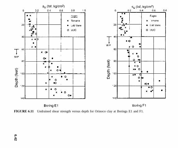
6.4
2
FIGURE 6.11 Undrained shear strength versus depth for Orinoco clay at Borings E1 and F1.
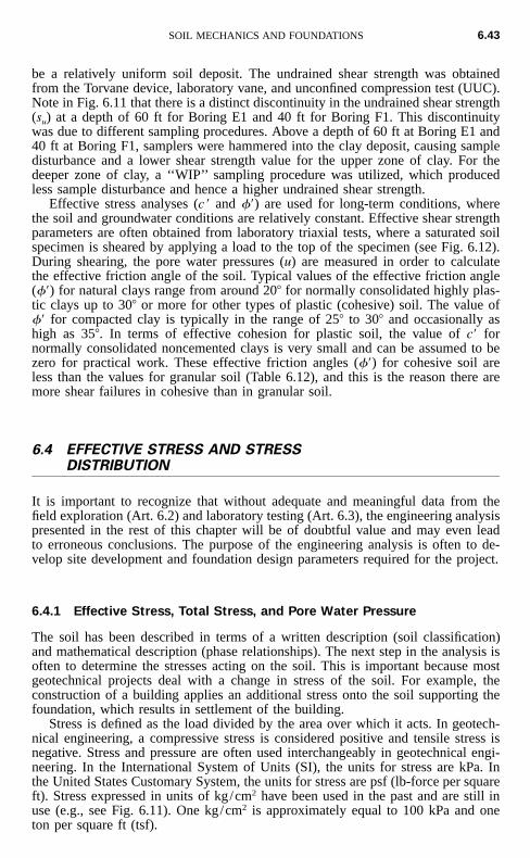
SOIL MECHANICS AND FOUNDATIONS 6.43
be a relatively uniform soil deposit. The undrained shear strength was obtainedfrom the Torvane device, laboratory vane, and unconfined compression test (UUC).Note in Fig. 6.11 that there is a distinct discontinuity in the undrained shear strength(su) at a depth of 60 ft for Boring E1 and 40 ft for Boring F1. This discontinuitywas due to different sampling procedures. Above a depth of 60 ft at Boring E1 and40 ft at Boring F1, samplers were hammered into the clay deposit, causing sampledisturbance and a lower shear strength value for the upper zone of clay. For thedeeper zone of clay, a ‘‘WIP’’ sampling procedure was utilized, which producedless sample disturbance and hence a higher undrained shear strength.
Effective stress analyses (c � and ��) are used for long-term conditions, wherethe soil and groundwater conditions are relatively constant. Effective shear strengthparameters are often obtained from laboratory triaxial tests, where a saturated soilspecimen is sheared by applying a load to the top of the specimen (see Fig. 6.12).During shearing, the pore water pressures (u) are measured in order to calculatethe effective friction angle of the soil. Typical values of the effective friction angle(��) for natural clays range from around 20� for normally consolidated highly plas-tic clays up to 30� or more for other types of plastic (cohesive) soil. The value of�� for compacted clay is typically in the range of 25� to 30� and occasionally ashigh as 35�. In terms of effective cohesion for plastic soil, the value of c� fornormally consolidated noncemented clays is very small and can be assumed to bezero for practical work. These effective friction angles (��) for cohesive soil areless than the values for granular soil (Table 6.12), and this is the reason there aremore shear failures in cohesive than in granular soil.
6.4 EFFECTIVE STRESS AND STRESSDISTRIBUTION
It is important to recognize that without adequate and meaningful data from thefield exploration (Art. 6.2) and laboratory testing (Art. 6.3), the engineering analysispresented in the rest of this chapter will be of doubtful value and may even leadto erroneous conclusions. The purpose of the engineering analysis is often to de-velop site development and foundation design parameters required for the project.
6.4.1 Effective Stress, Total Stress, and Pore Water Pressure
The soil has been described in terms of a written description (soil classification)and mathematical description (phase relationships). The next step in the analysis isoften to determine the stresses acting on the soil. This is important because mostgeotechnical projects deal with a change in stress of the soil. For example, theconstruction of a building applies an additional stress onto the soil supporting thefoundation, which results in settlement of the building.
Stress is defined as the load divided by the area over which it acts. In geotech-nical engineering, a compressive stress is considered positive and tensile stress isnegative. Stress and pressure are often used interchangeably in geotechnical engi-neering. In the International System of Units (SI), the units for stress are kPa. Inthe United States Customary System, the units for stress are psf (lb-force per squareft). Stress expressed in units of kg/cm2 have been used in the past and are still inuse (e.g., see Fig. 6.11). One kg/cm2 is approximately equal to 100 kPa and oneton per square ft (tsf).
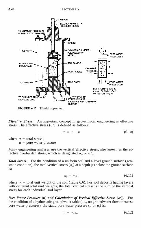
6.44 SECTION SIX
FIGURE 6.12 Triaxial apparatus.
Effective Stress. An important concept in geotechnical engineering is effectivestress. The effective stress (�) is defined as follows:
� � � u (6.10)
where � total stressu � pore water pressure
Many engineering analyses use the vertical effective stress, also known as the ef-fective overburden stress, which is designated or .� �v vo
Total Stress. For the condition of a uniform soil and a level ground surface (geo-static condition), the total vertical stress (v) at a depth (z) below the ground surfaceis:
� � z (6.11)v t
where �t � total unit weight of the soil (Table 6.6). For soil deposits having layerswith different total unit weights, the total vertical stress is the sum of the verticalstress for each individual soil layer.
Pore Water Pressure (u) and Calculation of Vertical Effective Stress (� ). For�vthe condition of a hydrostatic groundwater table (i.e., no groundwater flow or excesspore water pressures), the static pore water pressure (u or us) is:
u � � z (6.12)w w
SOIL MECHANICS AND FOUNDATIONS 6.45
where �w � unit weight of waterzw � depth below the groundwater table
If the total unit weight of the soil (Eq. 6.11), and the pore water pressure (Eq.6.12) are known, then the vertical effective stress ( ) can be calculated. An alter-�vnative method is to use the buoyant unit weight (�b , see Table 6.6) to calculate thevertical effective stress. For example, suppose that a groundwater table correspondswith the ground surface. In this case, the vertical effective stress ( ) is simply the�vbuoyant unit weight (�b) times the depth below the ground surface. More often, thegroundwater table is below the ground surface, in which case the vertical total stressof the soil layer above the groundwater table must be added to the buoyant unitweight calculations.
6.4.2 Stress Distribution
The previous section described methods used to determine the existing stresseswithin the soil mass. This section describes commonly used methods to determinethe increase in stress in the soil deposit due to applied loads. This is naturallyimportant in settlement analysis because the settlement of the structure is due di-rectly to its weight, which causes an increase in stress in the underlying soil. Inmost cases, it is the increase in vertical stress that is of most importance in settle-ment analyses. The symbol z is often used to denote an increase in vertical stressin the soil, although �v (change in total vertical stress) is also used.
When dealing with stress distribution, a distinction must be made between one-dimensional and two- or three-dimensional loading. A one-dimensional loadingapplies a stress increase at depth that is 100% of the applied surface stress. Anexample of a one-dimensional loading would be the placement of a fill layer ofuniform thickness and large areal extent at ground surface. Beneath the center ofthe uniform fill, the in-situ soil is subjected to an increase in vertical stress thatequals the following:
� � � h� (6.13)z v t
where h � thickness of the fill layer�t � total unit weight of the fill
In this case of one-dimensional loading, the soil would only be compressed in thevertical direction (i.e., strain only in the vertical direction).
Another example of one-dimensional loading is the uniform lowering of agroundwater table. If the total unit weight of the soil does not change as the ground-water table is lowered, then the one-dimensional increase in vertical stress for thein-situ soil located below the groundwater table would equal the following:
� � � h� (6.14)z v w
where h � vertical distance that the groundwater table is uniformly lowered�w � unit weight of water
Surface loadings can cause both vertical and horizontal strains, and this is re-ferred to as two- or three-dimensional loading. Common examples of two-dimensional loading are from strip footings or long embankments (i.e., plane strainconditions). Examples of three-dimensional loading would be square and rectan-
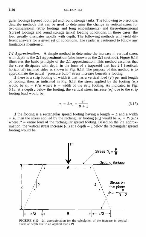
6.46 SECTION SIX
FIGURE 6.13 2:1 approximation for the calculation of the increase in verticalstress at depth due to an applied load (P).
gular footings (spread footings) and round storage tanks. The following two sectionsdescribe methods that can be used to determine the change in vertical stress fortwo-dimensional (strip footings and long embankments) and three-dimensional(spread footings and round storage tanks) loading conditions. In these cases, theload usually dissipates rapidly with depth. The following methods will yield dif-ferent answers for a given set of conditions. The reader is cautioned to follow anylimitations mentioned.
2:1 Approximation. A simple method to determine the increase in vertical stresswith depth is the 2:1 approximation (also known as the 2:1 method). Figure 6.13illustrates the basic principle of the 2:1 approximation. This method assumes thatthe stress dissipates with depth in the form of a trapezoid that has 2:1 (vertical:horizontal) inclined sides as shown in Fig. 6.13. The purpose of this method is toapproximate the actual ‘‘pressure bulb’’ stress increase beneath a footing.
If there is a strip footing of width B that has a vertical load (P) per unit lengthof footing, then, as indicated in Fig. 6.13, the stress applied by the footing (o)would be o � P /B where B � width of the strip footing. As indicated in Fig.6.13, at a depth z below the footing, the vertical stress increase (z) due to the stripfooting load would be:
P � � � (6.15)z v B � z
If the footing is a rectangular spread footing having a length � L and a width� B, then the stress applied by the rectangular footing (o) would be o � P / (BL)where P � entire load of the rectangular spread footing. Based on the 2:1 approx-imation, the vertical stress increase (z) at a depth � z below the rectangular spreadfooting would be:
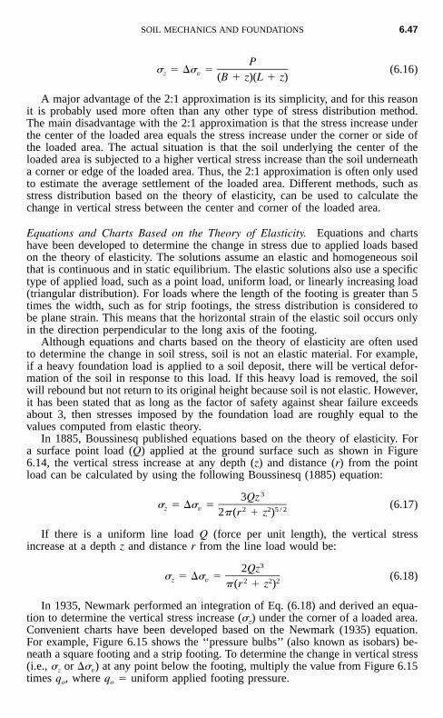
SOIL MECHANICS AND FOUNDATIONS 6.47
P � � � (6.16)z v (B � z)(L � z)
A major advantage of the 2:1 approximation is its simplicity, and for this reasonit is probably used more often than any other type of stress distribution method.The main disadvantage with the 2:1 approximation is that the stress increase underthe center of the loaded area equals the stress increase under the corner or side ofthe loaded area. The actual situation is that the soil underlying the center of theloaded area is subjected to a higher vertical stress increase than the soil underneatha corner or edge of the loaded area. Thus, the 2:1 approximation is often only usedto estimate the average settlement of the loaded area. Different methods, such asstress distribution based on the theory of elasticity, can be used to calculate thechange in vertical stress between the center and corner of the loaded area.
Equations and Charts Based on the Theory of Elasticity. Equations and chartshave been developed to determine the change in stress due to applied loads basedon the theory of elasticity. The solutions assume an elastic and homogeneous soilthat is continuous and in static equilibrium. The elastic solutions also use a specifictype of applied load, such as a point load, uniform load, or linearly increasing load(triangular distribution). For loads where the length of the footing is greater than 5times the width, such as for strip footings, the stress distribution is considered tobe plane strain. This means that the horizontal strain of the elastic soil occurs onlyin the direction perpendicular to the long axis of the footing.
Although equations and charts based on the theory of elasticity are often usedto determine the change in soil stress, soil is not an elastic material. For example,if a heavy foundation load is applied to a soil deposit, there will be vertical defor-mation of the soil in response to this load. If this heavy load is removed, the soilwill rebound but not return to its original height because soil is not elastic. However,it has been stated that as long as the factor of safety against shear failure exceedsabout 3, then stresses imposed by the foundation load are roughly equal to thevalues computed from elastic theory.
In 1885, Boussinesq published equations based on the theory of elasticity. Fora surface point load (Q) applied at the ground surface such as shown in Figure6.14, the vertical stress increase at any depth (z) and distance (r) from the pointload can be calculated by using the following Boussinesq (1885) equation:
33Qz � � � (6.17)z v 2 2 5 / 22� (r � z )
If there is a uniform line load Q (force per unit length), the vertical stressincrease at a depth z and distance r from the line load would be:
32Qz � � � (6.18)z v 2 2 2� (r � z )
In 1935, Newmark performed an integration of Eq. (6.18) and derived an equa-tion to determine the vertical stress increase (z) under the corner of a loaded area.Convenient charts have been developed based on the Newmark (1935) equation.For example, Figure 6.15 shows the ‘‘pressure bulbs’’ (also known as isobars) be-neath a square footing and a strip footing. To determine the change in vertical stress(i.e., z or �v) at any point below the footing, multiply the value from Figure 6.15times qo, where qo � uniform applied footing pressure.
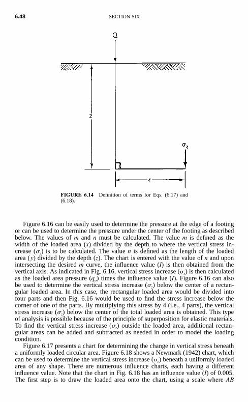
6.48 SECTION SIX
FIGURE 6.14 Definition of terms for Eqs. (6.17) and(6.18).
Figure 6.16 can be easily used to determine the pressure at the edge of a footingor can be used to determine the pressure under the center of the footing as describedbelow. The values of m and n must be calculated. The value m is defined as thewidth of the loaded area (x) divided by the depth to where the vertical stress in-crease (z) is to be calculated. The value n is defined as the length of the loadedarea (y) divided by the depth (z). The chart is entered with the value of n and uponintersecting the desired m curve, the influence value (I) is then obtained from thevertical axis. As indicated in Fig. 6.16, vertical stress increase (z) is then calculatedas the loaded area pressure (qo) times the influence value (I). Figure 6.16 can alsobe used to determine the vertical stress increase (z) below the center of a rectan-gular loaded area. In this case, the rectangular loaded area would be divided intofour parts and then Fig. 6.16 would be used to find the stress increase below thecorner of one of the parts. By multiplying this stress by 4 (i.e., 4 parts), the verticalstress increase (z) below the center of the total loaded area is obtained. This typeof analysis is possible because of the principle of superposition for elastic materials.To find the vertical stress increase (z) outside the loaded area, additional rectan-gular areas can be added and subtracted as needed in order to model the loadingcondition.
Figure 6.17 presents a chart for determining the change in vertical stress beneatha uniformly loaded circular area. Figure 6.18 shows a Newmark (1942) chart, whichcan be used to determine the vertical stress increase (z) beneath a uniformly loadedarea of any shape. There are numerous influence charts, each having a differentinfluence value. Note that the chart in Fig. 6.18 has an influence value (I) of 0.005.The first step is to draw the loaded area onto the chart, using a scale where AB
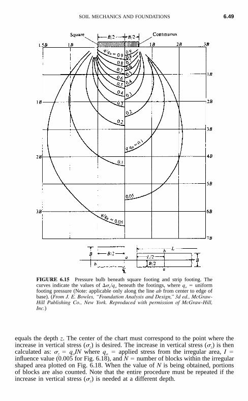
SOIL MECHANICS AND FOUNDATIONS 6.49
FIGURE 6.15 Pressure bulb beneath square footing and strip footing. Thecurves indicate the values of � /qo beneath the footings, where qo � uniformvfooting pressure (Note: applicable only along the line ab from center to edge ofbase). (From J. E. Bowles, ‘‘Foundation Analysis and Design,’’ 3d ed., McGraw-Hill Publishing Co., New York. Reproduced with permission of McGraw-Hill,Inc.)
equals the depth z. The center of the chart must correspond to the point where theincrease in vertical stress (z) is desired. The increase in vertical stress (z) is thencalculated as: z � qoIN where qo � applied stress from the irregular area, I �influence value (0.005 for Fig. 6.18), and N � number of blocks within the irregularshaped area plotted on Fig. 6.18. When the value of N is being obtained, portionsof blocks are also counted. Note that the entire procedure must be repeated if theincrease in vertical stress (z) is needed at a different depth.
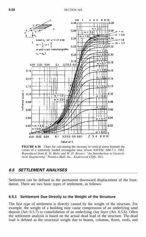
6.50 SECTION SIX
FIGURE 6.16 Chart for calculating the increase in vertical stress beneath thecorner of a uniformly loaded rectangular area. (From NAVFAC DM-7.1, 1982,Reproduced from R. D. Holtz and W. D. Kovacs, ‘‘An Introduction to Geotech-nical Engineering,’’ Prentice-Hall, Inc., Englewood Cliffs, NJ.)
6.5 SETTLEMENT ANALYSES
Settlement can be defined as the permanent downward displacement of the foun-dation. There are two basic types of settlement, as follows:
6.5.1 Settlement Due Directly to the Weight of the Structure
The first type of settlement is directly caused by the weight of the structure. Forexample, the weight of a building may cause compression of an underlying sanddeposit (Art. 6.5.7) or consolidation of an underlying clay layer (Art. 6.5.6). Oftenthe settlement analysis is based on the actual dead load of the structure. The deadload is defined as the structural weight due to beams, columns, floors, roofs, and
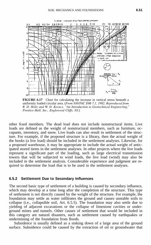
SOIL MECHANICS AND FOUNDATIONS 6.51
FIGURE 6.17 Chart for calculating the increase in vertical stress beneath auniformly loaded circular area. (From NAVFAC DM-7.1, 1982, Reproduced fromR. D. Holtz and W. D. Kovacs, ‘‘An Introduction to Geotechnical Engineering,’’Prentice-Hall, Inc., Englewood Cliffs, NJ.)
other fixed members. The dead load does not include nonstructural items. Liveloads are defined as the weight of nonstructural members, such as furniture, oc-cupants, inventory, and snow. Live loads can also result in settlement of the struc-ture. For example, if the proposed structure is a library, then the actual weight ofthe books (a live load) should be included in the settlement analyses. Likewise, fora proposed warehouse, it may be appropriate to include the actual weight of antic-ipated stored items in the settlement analyses. In other projects where the live loadsrepresent a significant part of the loading, such as large electrical transmissiontowers that will be subjected to wind loads, the live load (wind) may also beincluded in the settlement analysis. Considerable experience and judgment are re-quired to determine the load that is to be used in the settlement analyses.
6.5.2 Settlement Due to Secondary Influences
The second basic type of settlement of a building is caused by secondary influence,which may develop at a time long after the completion of the structure. This typeof settlement is not directly caused by the weight of the structure. For example, thefoundation may settle as water infiltrates the ground and causes unstable soils tocollapse (i.e., collapsible soil, Art. 6.5.5). The foundation may also settle due toyielding of adjacent excavations or the collapse of limestone cavities or under-ground mines and tunnels. Other causes of settlement that would be included inthis category are natural disasters, such as settlement caused by earthquakes orundermining of the foundation from floods.
Subsidence is usually defined as a sinking down of a large area of the groundsurface. Subsidence could be caused by the extraction of oil or groundwater that
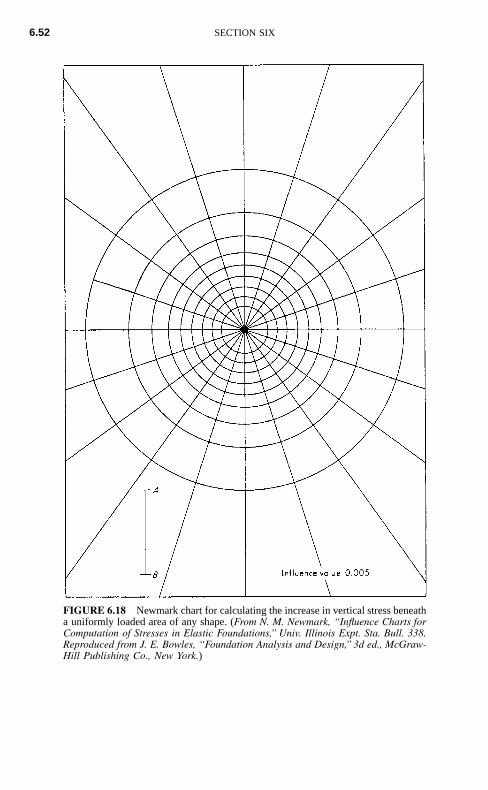
6.52 SECTION SIX
FIGURE 6.18 Newmark chart for calculating the increase in vertical stress beneatha uniformly loaded area of any shape. (From N. M. Newmark, ‘‘Influence Charts forComputation of Stresses in Elastic Foundations,’’ Univ. Illinois Expt. Sta. Bull. 338.Reproduced from J. E. Bowles, ‘‘Foundation Analysis and Design,’’ 3d ed., McGraw-Hill Publishing Co., New York.)
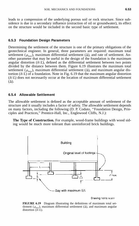
SOIL MECHANICS AND FOUNDATIONS 6.53
FIGURE 6.19 Diagram illustrating the definitions of maximum total set-tlement (�max), maximum differential settlement (�), and maximum angulardistortion (� / L).
leads to a compression of the underlying porous soil or rock structure. Since sub-sidence is due to a secondary influence (extraction of oil or groundwater), its effecton the structure would be included in the second basic type of settlement.
6.5.3 Foundation Design Parameters
Determining the settlement of the structure is one of the primary obligations of thegeotechnical engineer. In general, three parameters are required: maximum totalsettlement (�max), maximum differential settlement (�), and rate of settlement. An-other parameter that may be useful in the design of the foundation is the maximumangular distortion (� /L), defined as the differential settlement between two pointsdivided by the distance between them. Figure 6.19 illustrates the maximum totalsettlement (�max), maximum differential settlement (�), and maximum angular dis-tortion (� /L) of a foundation. Note in Fig. 6.19 that the maximum angular distortion(� /L) does not necessarily occur at the location of maximum differential settlement(�).
6.5.4 Allowable Settlement
The allowable settlement is defined as the acceptable amount of settlement of thestructure and it usually includes a factor of safety. The allowable settlement dependson many factors, including the following (D. P. Coduto, ‘‘Foundation Design, Prin-ciples and Practices,’’ Prentice-Hall, Inc., Englewood Cliffs, N.J.):
The Type of Construction. For example, wood-frame buildings with wood sid-ing would be much more tolerant than unreinforced brick buildings.
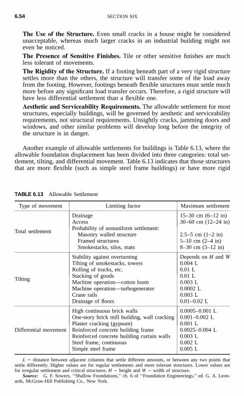
6.54 SECTION SIX
TABLE 6.13 Allowable Settlement
Type of movement Limiting factor Maximum settlement
Total settlement
DrainageAccessProbability of nonuniform settlement:
Masonry walled structureFramed structuresSmokestacks, silos, mats
15–30 cm (6–12 in)30–60 cm (12–24 in)
2.5–5 cm (1–2 in)5–10 cm (2–4 in)8–30 cm (3–12 in)
Tilting
Stability against overturningTilting of smokestacks, towersRolling of trucks, etc.Stacking of goodsMachine operation—cotton loomMachine operation—turbogeneratorCrane railsDrainage of floors
Depends on H and W0.004 L0.01 L0.01 L0.003 L0.0002 L0.003 L0.01–0.02 L
Differential movement
High continuous brick wallsOne-story brick mill building, wall crackingPlaster cracking (gypsum)Reinforced concrete building frameReinforced concrete building curtain wallsSteel frame, continuousSimple steel frame
0.0005–0.001 L0.001–0.002 L0.001 L0.0025–0.004 L0.003 L0.002 L0.005 L
L � distance between adjacent columns that settle different amounts, or between any two points thatsettle differently. Higher values are for regular settlements and more tolerant structures. Lower values arefor irregular settlement and critical structures. H � height and W � width of structure.
Source: G. F. Sowers, ‘‘Shallow Foundations,’’ ch. 6 of ‘‘Foundation Engineerings,’’ ed. G. A. Leon-ards, McGraw-Hill Publishing Co., New York.
The Use of the Structure. Even small cracks in a house might be consideredunacceptable, whereas much larger cracks in an industrial building might noteven be noticed.The Presence of Sensitive Finishes. Tile or other sensitive finishes are muchless tolerant of movements.The Rigidity of the Structure. If a footing beneath part of a very rigid structuresettles more than the others, the structure will transfer some of the load awayfrom the footing. However, footings beneath flexible structures must settle muchmore before any significant load transfer occurs. Therefore, a rigid structure willhave less differential settlement than a flexible one.Aesthetic and Serviceability Requirements. The allowable settlement for moststructures, especially buildings, will be governed by aesthetic and serviceabilityrequirements, not structural requirements. Unsightly cracks, jamming doors andwindows, and other similar problems will develop long before the integrity ofthe structure is in danger.
Another example of allowable settlements for buildings is Table 6.13, where theallowable foundation displacement has been divided into three categories: total set-tlement, tilting, and differential movement. Table 6.13 indicates that those structuresthat are more flexible (such as simple steel frame buildings) or have more rigid
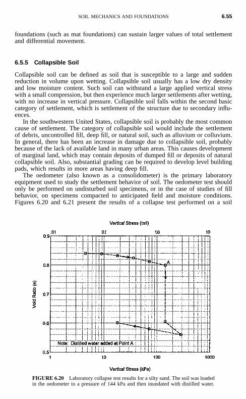
SOIL MECHANICS AND FOUNDATIONS 6.55
FIGURE 6.20 Laboratory collapse test results for a silty sand. The soil was loadedin the oedometer to a pressure of 144 kPa and then inundated with distilled water.
foundations (such as mat foundations) can sustain larger values of total settlementand differential movement.
6.5.5 Collapsible Soil
Collapsible soil can be defined as soil that is susceptible to a large and suddenreduction in volume upon wetting. Collapsible soil usually has a low dry densityand low moisture content. Such soil can withstand a large applied vertical stresswith a small compression, but then experience much larger settlements after wetting,with no increase in vertical pressure. Collapsible soil falls within the second basiccategory of settlement, which is settlement of the structure due to secondary influ-ences.
In the southwestern United States, collapsible soil is probably the most commoncause of settlement. The category of collapsible soil would include the settlementof debris, uncontrolled fill, deep fill, or natural soil, such as alluvium or colluvium.In general, there has been an increase in damage due to collapsible soil, probablybecause of the lack of available land in many urban areas. This causes developmentof marginal land, which may contain deposits of dumped fill or deposits of naturalcollapsible soil. Also, substantial grading can be required to develop level buildingpads, which results in more areas having deep fill.
The oedometer (also known as a consolidometer) is the primary laboratoryequipment used to study the settlement behavior of soil. The oedometer test shouldonly be performed on undisturbed soil specimens, or in the case of studies of fillbehavior, on specimens compacted to anticipated field and moisture conditions.Figures 6.20 and 6.21 present the results of a collapse test performed on a soil
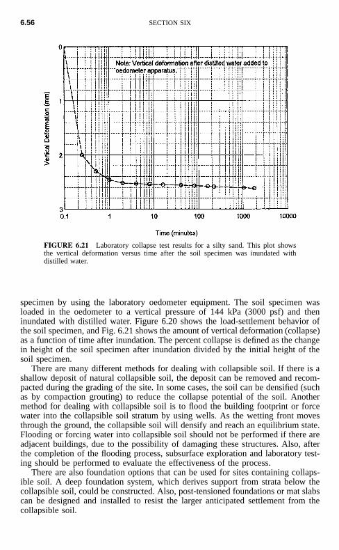
6.56 SECTION SIX
FIGURE 6.21 Laboratory collapse test results for a silty sand. This plot showsthe vertical deformation versus time after the soil specimen was inundated withdistilled water.
specimen by using the laboratory oedometer equipment. The soil specimen wasloaded in the oedometer to a vertical pressure of 144 kPa (3000 psf) and theninundated with distilled water. Figure 6.20 shows the load-settlement behavior ofthe soil specimen, and Fig. 6.21 shows the amount of vertical deformation (collapse)as a function of time after inundation. The percent collapse is defined as the changein height of the soil specimen after inundation divided by the initial height of thesoil specimen.
There are many different methods for dealing with collapsible soil. If there is ashallow deposit of natural collapsible soil, the deposit can be removed and recom-pacted during the grading of the site. In some cases, the soil can be densified (suchas by compaction grouting) to reduce the collapse potential of the soil. Anothermethod for dealing with collapsible soil is to flood the building footprint or forcewater into the collapsible soil stratum by using wells. As the wetting front movesthrough the ground, the collapsible soil will densify and reach an equilibrium state.Flooding or forcing water into collapsible soil should not be performed if there areadjacent buildings, due to the possibility of damaging these structures. Also, afterthe completion of the flooding process, subsurface exploration and laboratory test-ing should be performed to evaluate the effectiveness of the process.
There are also foundation options that can be used for sites containing collaps-ible soil. A deep foundation system, which derives support from strata below thecollapsible soil, could be constructed. Also, post-tensioned foundations or mat slabscan be designed and installed to resist the larger anticipated settlement from thecollapsible soil.
SOIL MECHANICS AND FOUNDATIONS 6.57
6.5.6 Settlement of Cohesive and Organic Soils
Cohesive and organic soil can be susceptible to a large amount of settlement fromstructural loads. It is usually the direct weight of the structure that causes settlementof the cohesive or organic soil. The settlement of saturated clay or organic soil canhave three different components: immediate (also known as ‘‘initial settlement’’),primary consolidation, and secondary compression.
Immediate Settlement. In most situations, surface loading causes both vertical andhorizontal strains. This is referred to as two- or three-dimensional loading. Imme-diate settlement is due to undrained shear deformations, or in some cases containedplastic flow, caused by the two- or three-dimensional loading. Common examplesof three-dimensional loading are from square footings and round storage tanks.Many different methods are available to determine the amount of immediate settle-ment for two- or three-dimensional loadings. Examples include field plate load tests,equations based on the theory of elasticity, and the stress path method (see R. W.Day, ‘‘Geotechnical and Foundation Engineering: Design and Construction,’’ Mc-Graw-Hill Publishing Co., New York).
Primary Consolidation. The increase in vertical pressure due to the weight of thestructure constructed on top of saturated soft clays and organic soil will initially becarried by the pore water in the soil. This increase in pore water pressure is knownas an excess pore water pressure (ue). The excess pore water pressure will decreasewith time as water slowly flows out of the cohesive soil. This flow of water fromcohesive soil (which has a low permeability) as the excess pore water pressuresslowly dissipate is known as primary consolidation, or simply consolidation. Asthe water slowly flows from the cohesive soil, the structure settles as the load istransferred to the soil particle skeleton, thereby increasing the effective stress ofthe soil. Consolidation is a time-dependent process that may take many years tocomplete.
Based on the stress history of saturated cohesive soils, they are considered tobe either underconsolidated, normally consolidated, or overconsolidated. The over-consolidation ratio (OCR) is used to describe the stress history of cohesive soil,and it is defined as: OCR � / , where: or � maximum past pressure� � � �vm vo vm p
( ), also known as the preconsolidation pressure ( ), which is equal to the� �vm p
highest previous vertical effective stress that the cohesive soil was subjected to andconsolidated under, and or � existing vertical effective stress. In terms of� �vo vthe stress history of a cohesive soil, there are three possible conditions:
1. Underconsolidated (OCR � 1). A saturated cohesive soil is considered under-consolidated if the soil is not fully consolidated under the existing overburdenpressure and excess pore water pressures (ue) exist within the soil. Undercon-solidation occurs in areas where a cohesive soil is being deposited very rapidlyand not enough time has elapsed for the soil to consolidate under its own weight.
2. Normally Consolidated (OCR � 1). A saturated cohesive soil is considerednormally consolidated if it has never been subjected to an effective stress greaterthan the existing overburden pressure and if the deposit is completely consoli-dated under the existing overburden pressure.
3. Overconsolidated or Preconsolidated (OCR � 1): A saturated cohesive soil isconsidered overconsolidated if it has been subjected in the past to a vertical
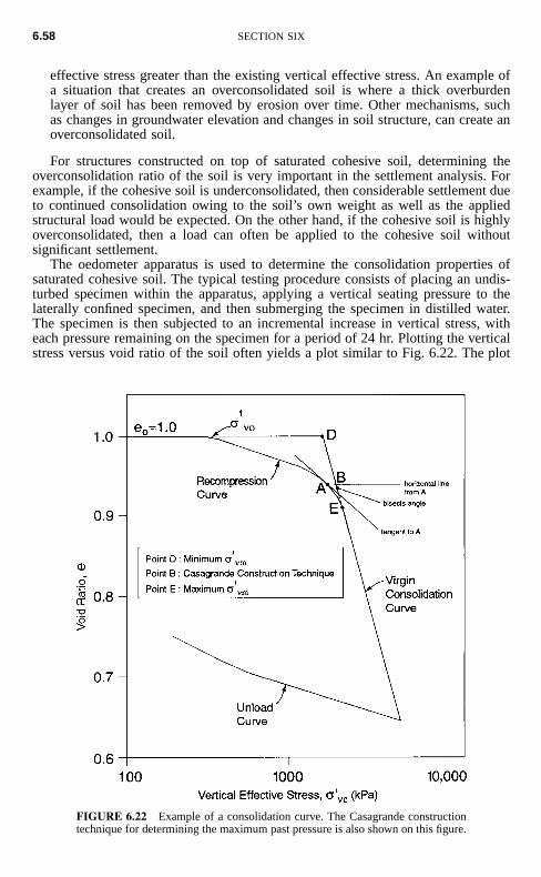
6.58 SECTION SIX
FIGURE 6.22 Example of a consolidation curve. The Casagrande constructiontechnique for determining the maximum past pressure is also shown on this figure.
effective stress greater than the existing vertical effective stress. An example ofa situation that creates an overconsolidated soil is where a thick overburdenlayer of soil has been removed by erosion over time. Other mechanisms, suchas changes in groundwater elevation and changes in soil structure, can create anoverconsolidated soil.
For structures constructed on top of saturated cohesive soil, determining theoverconsolidation ratio of the soil is very important in the settlement analysis. Forexample, if the cohesive soil is underconsolidated, then considerable settlement dueto continued consolidation owing to the soil’s own weight as well as the appliedstructural load would be expected. On the other hand, if the cohesive soil is highlyoverconsolidated, then a load can often be applied to the cohesive soil withoutsignificant settlement.
The oedometer apparatus is used to determine the consolidation properties ofsaturated cohesive soil. The typical testing procedure consists of placing an undis-turbed specimen within the apparatus, applying a vertical seating pressure to thelaterally confined specimen, and then submerging the specimen in distilled water.The specimen is then subjected to an incremental increase in vertical stress, witheach pressure remaining on the specimen for a period of 24 hr. Plotting the verticalstress versus void ratio of the soil often yields a plot similar to Fig. 6.22. The plot
SOIL MECHANICS AND FOUNDATIONS 6.59
is known as the consolidation curve and consists of two important segments, therecompression curve (defined by the recompression index Cr) and the virgin con-solidation curve (defined by the compression index Cc). Figure 6.22 also illustratesthe Casagrande construction technique, which can be used to determine the maxi-mum past pressure ( ).�vm
Using the calculated values of Cr and Cc , the primary consolidation settlement(sc) due to an increase in load (�v) can be determined from the following equa-tions:
1. For underconsolidated soil (OCR � 1):
H � � �� � �o vo v vs � C log (6.19)c c 1 � e �o vo
2. For normally consolidated soil (OCR � 1):
H � � �o vo vs � C log (6.20)c c 1 � e �o vo
3. For overconsolidated soil (OCR � 1):Case I: � �� � �vo v vm
H � � �o vo vs � C log (6.21)c r 1 � e �o vo
Case II: � � � � �vo v vm
H � H � � �o vm o vo vs � C log � C log (6.22)c r c1 � e � 1 � e �o vo o vm
where sc � settlement due to primary consolidation caused by an increase inload
Cc � compression index, obtained from the virgin consolidation curve(Fig. 6.22)
Cr � recompression index, obtained from the recompression portion ofthe consolidation curve (Fig. 6.22)
Ho � initial thickness of the in-situ saturated cohesive soil layereo � initial void ratio of the in-situ saturated cohesive soil layer
��vo initial vertical effective stress of the in-situ soil (see Art. 6.4.1)� ��v for an underconsolidated soil (this represents the increase in vertical
effective stress that will occur as the cohesive soil consolidates underits own weight)
��vm maximum past pressure, also known as the preconsolidation pressure( ), which is obtained from the consolidation curve using the Cas-�pagrande construction technique (see Fig. 6.22)
�v � increase in load, typically due to the construction of a building orthe construction of a fill layer at ground surface
The value of �v (also known as z) can be obtained from stress distributiontheory as discussed in Art. 6.4.2. Note that a drop in the groundwater table or areduction in pore water pressure can also result in an increase in load on the co-hesive soil.
6.60 SECTION SIX
For overconsolidated soil, there are two possible cases that can be used to cal-culate the amount of settlement. The first case occurs when the existing verticaleffective stress ( ) plus the increase in vertical stress (�v) due to the proposed�vo
building weight does not exceed the maximum past pressure ( ). For this first�vm
case, there will only be recompression of the cohesive soil.For the second case, the sum of the existing vertical effective stress ( ) plus�vo
the increase in vertical stress (�v) due to the proposed building weight exceedsthe maximum past pressure ( ). For the second case, there will be virgin con-�vm
solidation of the cohesive soil. Given the same cohesive soil and identical fieldconditions, the settlement due to the second case will be significantly more thanthe first case.
As previously mentioned, primary consolidation is a time-dependent process thatcan take many years to complete. The rate of consolidation can be estimated usingthe Terzaghi theory of consolidation (see K. Terzaghi and R. B. Peck, ‘‘Soil Me-chanics in Engineering Practice,’’ John Wiley & Sons, Inc., New York):
Secondary Compression. The final component of settlement is due to secondarycompression, which is that part of the settlement that occurs after essentially all ofthe excess pore water pressures have dissipated (i.e., settlement that occurs at con-stant effective stress). The usual assumption is that secondary compression does notstart until after primary consolidation is complete. The amount of secondary com-pression is often neglected because it is rather small compared to the primaryconsolidation settlement. However, secondary compression can constitute a majorpart of the total settlement for peat or other highly organic soil (see R. D. Holtzand W. D. Kovacs, ‘‘An Introduction to Geotechnical Engineering,’’ Prentice-Hall,Inc., Englewood Cliffs, NJ).
The final calculation for estimating the maximum settlement (�max) of the in-situ cohesive soil would be to add together the three components of settlement, or:
� � s � s � s (6.23)max i c s
where �max � maximum settlement over the life of the structuresi � immediate settlementsc � primary consolidation settlementss � secondary compression settlement
6.5.7 Settlement of Granular Soil
A major difference between saturated cohesive soil and granular soil is that thesettlement of cohesionless soil is not time dependent. Because of the generally highpermeability of granular soil, the settlement usually occurs as the load is appliedduring the construction of the building. Many different methods can be used todetermine the settlement of granular soil, such as plate load tests, laboratory testingof undisturbed soil samples, equations based on the theory of elasticity, and em-pirical correlations. For example, Fig. 6.23 shows a chart that presents an empiricalcorrelation between the measured N value (obtained from the Standard PenetrationTest, see Art. 6.2.4) and the allowable soil pressure (tsf) that will produce a settle-ment of the footing of 1 in (2.5 cm).
As an example of the use of Fig. 6.23, suppose a site contains a sand depositand the proposed structure can be subjected to a maximum settlement (�max) of1.0 in (2.5 cm). If the measured N value from the Standard Penetration Test � 10and the width of the proposed footings � 5 ft (1.5 m), then the allowable soilpressure � 1 tsf (100 kPa).
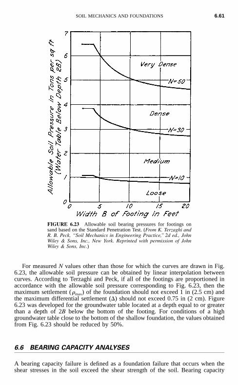
SOIL MECHANICS AND FOUNDATIONS 6.61
FIGURE 6.23 Allowable soil bearing pressures for footings onsand based on the Standard Penetration Test. (From K. Terzaghi andR. B. Peck, ‘‘Soil Mechanics in Engineering Practice,’’ 2d ed., JohnWiley & Sons, Inc., New York. Reprinted with permission of JohnWiley & Sons, Inc.)
For measured N values other than those for which the curves are drawn in Fig.6.23, the allowable soil pressure can be obtained by linear interpolation betweencurves. According to Terzaghi and Peck, if all of the footings are proportioned inaccordance with the allowable soil pressure corresponding to Fig. 6.23, then themaximum settlement (�max) of the foundation should not exceed 1 in (2.5 cm) andthe maximum differential settlement (�) should not exceed 0.75 in (2 cm). Figure6.23 was developed for the groundwater table located at a depth equal to or greaterthan a depth of 2B below the bottom of the footing. For conditions of a highgroundwater table close to the bottom of the shallow foundation, the values obtainedfrom Fig. 6.23 should be reduced by 50%.
6.6 BEARING CAPACITY ANALYSES
A bearing capacity failure is defined as a foundation failure that occurs when theshear stresses in the soil exceed the shear strength of the soil. Bearing capacity
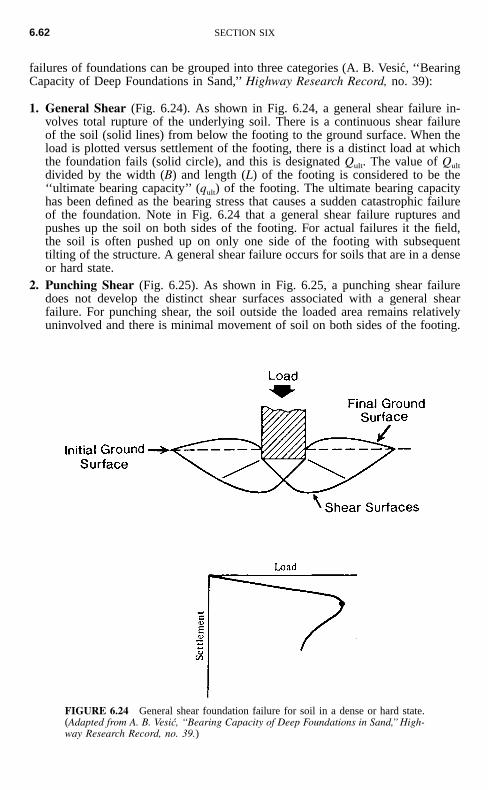
6.62 SECTION SIX
FIGURE 6.24 General shear foundation failure for soil in a dense or hard state.(Adapted from A. B. Vesic, ‘‘Bearing Capacity of Deep Foundations in Sand,’’ High-way Research Record, no. 39.)
failures of foundations can be grouped into three categories (A. B. Vesic, ‘‘BearingCapacity of Deep Foundations in Sand,’’ Highway Research Record, no. 39):
1. General Shear (Fig. 6.24). As shown in Fig. 6.24, a general shear failure in-volves total rupture of the underlying soil. There is a continuous shear failureof the soil (solid lines) from below the footing to the ground surface. When theload is plotted versus settlement of the footing, there is a distinct load at whichthe foundation fails (solid circle), and this is designated Qult. The value of Qult
divided by the width (B) and length (L) of the footing is considered to be the‘‘ultimate bearing capacity’’ (qult) of the footing. The ultimate bearing capacityhas been defined as the bearing stress that causes a sudden catastrophic failureof the foundation. Note in Fig. 6.24 that a general shear failure ruptures andpushes up the soil on both sides of the footing. For actual failures it the field,the soil is often pushed up on only one side of the footing with subsequenttilting of the structure. A general shear failure occurs for soils that are in a denseor hard state.
2. Punching Shear (Fig. 6.25). As shown in Fig. 6.25, a punching shear failuredoes not develop the distinct shear surfaces associated with a general shearfailure. For punching shear, the soil outside the loaded area remains relativelyuninvolved and there is minimal movement of soil on both sides of the footing.
SOIL MECHANICS AND FOUNDATIONS 6.63
FIGURE 6.25 Punching shear foundation failure for soilin a loose or soft state. (Adapted from A. B. Vesic, ‘‘BearingCapacity of Deep Foundations in Sand,’’ Highway Re-search Record, no. 39.)
The process of deformation of the footing involves compression of soil directlybelow the footing as well as the vertical shearing of soil around the footingperimeter. As shown in Fig. 6.25, the load settlement curve does not have adramatic break, and for punching shear, the bearing capacity is often defined asthe first major nonlinearity in the load-settlement curve (open circle). A punchingshear failure occurs for soils that are in a loose or soft state.
3. Local Shear Failure (Fig. 6.26). As shown in Fig. 6.26, local shear failureinvolves rupture of the soil only immediately below the footing. There is soilbulging on both sides of the footing, but the bulging is not as significant as ingeneral shear. Local shear failure can be considered as a transitional phase be-tween general shear and punching shear. Because of the transitional nature oflocal shear failure, the bearing capacity could be defined as the first major non-linearity in the load-settlement curve (open circle) or at the point where thesettlement rapidly increases (solid circle). A local shear failure occurs for soilsthat have a medium density or firm state.
The documented cases of bearing capacity failures indicate that usually the fol-lowing three factors (separately or in combination) are the cause of the failure:
6.64 SECTION SIX
FIGURE 6.26 Local shear foundation failure, which is a transitional phase be-tween general shear and punching shear failures. (Adapted from A. B. Vesic, ‘‘Bear-ing Capacity of Deep Foundations in Sand,’’ Highway Research Record, no. 39.)
1. There was an overestimation of the shear strength of the underlying soil.2. The actual structural load at the time of the bearing capacity failure was greater
than that assumed during the design phase.3. The site was altered, such as the construction of an adjacent excavation, which
resulted in a reduction in support and a bearing capacity failure.
A famous case of a bearing capacity failure is the Transcona grain elevator,located at Transcona, Manitoba, Canada, near Winnipeg. Figure 6.27 shows theOctober 1913 failure of the grain elevator. At the time of failure, the grain elevatorwas essentially fully loaded. The foundation had been constructed on clay that wasdescribed as a stiff clay. Note in Fig. 6.27 that the soil has been pushed up on onlyone side of the foundation, with subsequent tilting of the structure.
6.6.1 Bearing Capacity for Shallow Foundations
As indicated in Table 6.2, common types of shallow foundations include spreadfootings for isolated columns, combined footings for supporting the load from morethan one structural unit, strip footings for walls, and mats or raft foundations con-structed at or near ground surface. Shallow footings often have an embedment thatis less than the footing width.
SOIL MECHANICS AND FOUNDATIONS 6.65
FIGURE 6.27 Transcona grain elevator bearing capacity failure.
Bearing Capacity Equation. The most commonly used bearing capacity equationis the equation developed by Terzaghi (‘‘Theoretical Soil Mechanics,’’ John Wiley& Sons, Inc., New York). For a uniform vertical loading of a strip footing, Terzaghiassumed a general shear failure (Fig. 6.24) in order to develop the following bearingcapacity equation:
Qult 1q � � cN � ⁄2 � BN � � D N (6.24)ult c t � t ƒ qBL
where qult � ultimate bearing capacity for a strip footingQult � vertical load causing a general shear failure of the underlying soil
(Fig. 6.24)B � width of the strip footingL � length of the strip footing�t � total unit weight of the soil
Dƒ � vertical distance from the ground surface to the bottom of thestrip footing
c � cohesion of the soil underlying the strip footingNc, N�, and Nq � dimensionless bearing capacity factors
In order to calculate the allowable bearing pressure (qall), the following equationis used: qall � qult /F, where qall � allowable bearing pressure, qult � ultimate bearingcapacity from Eq. (6.24), and F � factor of safety (typically F � 3). This allowablebearing pressure often has to be reduced in order to prevent excessive settlementof the foundation. In addition, building codes often list allowable bearing pressuresversus soil or rock types, such as Table 6.14, which presents the allowable bearingpressures (qall) from the ‘‘Uniform Building Code’’ (1997).
6.66 SECTION SIX
TABLE 6.14 Allowable Bearing Pressures
Material typeAllowable bearing
pressureaMaximum allowable
bearing pressureb
Massive crystalline bedrock 4,000 psf (200 kPa) 12,000 psf (600 kPa)Sedimentary and foliated rock 2,000 psf (100 kPa) 6,000 psf (300 kPa)Gravel and sandy gravel (GW, GP) 2,000 psf (100 kPa) 6,000 psf (300 kPa)Nonplastic soil: sands, silts, and NP silt
(GM, SW, SP, SM)c1,500 psf (75 kPa) 4,500 psf (220 kPa)
Plastic soil: silts and clays (ML, MH, SC,CL, CH)c
1,000 psf (50 kPa) 3,000 psf (150 kPa)d
a Minimum footing width and embedment depth equals 1 ft (0.3 m).b An increase of 20% of the allowable bearing pressure is allowed for each additional foot (0.3 m) of
width or depth up to the maximum allowable bearing pressures listed in Column 3. An exception is plasticsoil, see note d.
c Group symbols from Table 6.8.d No increase in the allowable bearing pressure is allowed for an increase in width of the footing.For dense or stiff soils, allowable bearing values in this table are generally conservative. For very loose
or very soft soils, the allowable bearing values may be too high.Source: Data from ‘‘Uniform Building Code’’ (1997)
There are many charts, graphs, and figures that present bearing capacity factorsdeveloped by different engineers and researchers based on varying assumptions. Forexample, Fig. 6.28 presents bearing capacity factors Nc, N�, and Nq , which auto-matically incorporate allowance for punching and local shear failure. Another ex-ample is Fig. 6.29, which presents bearing capacity factors that have not beenadjusted for punching or local shear failure. Figure 6.29 also presents the bearingcapacity equations for square, rectangular, and circular footings. The equations forgranular soil (i.e., cohesionless soil, c � 0) and for a total stress analysis for co-hesive soil (i.e., � � 0 and c � su) are also shown in Fig. 6.29.
Other Footing Loads. In addition to the vertical load acting on the footing, itmay also be subjected to a lateral load. A common procedure is to treat lateralloads separately and resist the lateral loads by using the soil pressure acting on thesides of the footing (passive pressure) and the frictional resistance along the bottomof the footing.
It is always desirable to design and construct shallow footings so that the verticalload is applied at the center of gravity of the footing. For combined footings thatcarry more than one vertical load, the combined footing should be designed andconstructed so that the vertical loads are symmetric. There may be design situationswhere the footing is subjected to a moment, such as where there is a fixed-endconnection between the building frame and the footing. This moment can be rep-resented by a load Q that is offset a certain distance (known as the eccentricity)from the center of gravity of the footing. For other projects, there may be propertyline constraints and the load must be offset a certain distance (eccentricity) fromthe center of gravity of the footing. Because an eccentrically loaded footing willcreate a higher bearing pressure under one side as compared to the opposite side,one approach is to evaluate the actual pressure distribution beneath the footing. Theusual procedure is to assume a rigid footing (hence linear pressure distribution) anduse the section modulus (1⁄6B2) in order to calculate the largest and lowest bearingpressure. For a footing having a width B, the largest (q �) and lowest (q �) bearingpressures are as follows:
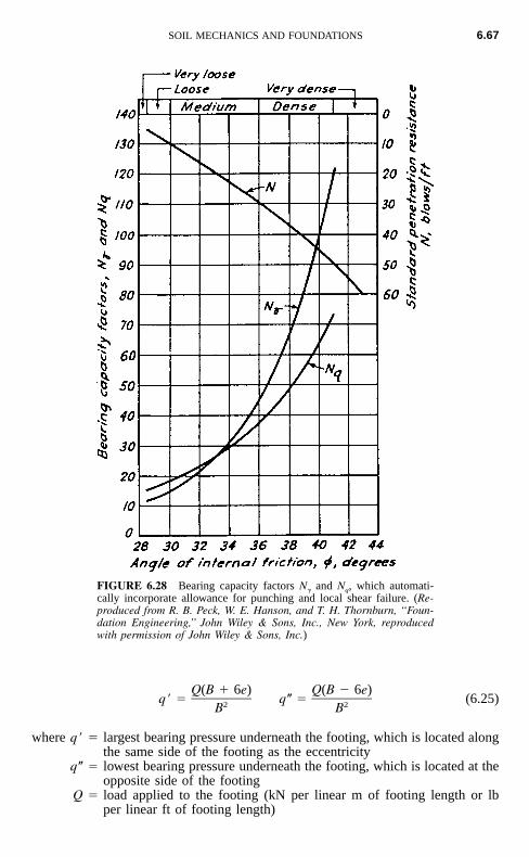
SOIL MECHANICS AND FOUNDATIONS 6.67
FIGURE 6.28 Bearing capacity factors N� and Nq, which automati-cally incorporate allowance for punching and local shear failure. (Re-produced from R. B. Peck, W. E. Hanson, and T. H. Thornburn, ‘‘Foun-dation Engineering,’’ John Wiley & Sons, Inc., New York, reproducedwith permission of John Wiley & Sons, Inc.)
Q(B � 6e) Q(B � 6e)q � � q � � (6.25)2 2B B
where q � � largest bearing pressure underneath the footing, which is located alongthe same side of the footing as the eccentricity
q � � lowest bearing pressure underneath the footing, which is located at theopposite side of the footing
Q � load applied to the footing (kN per linear m of footing length or lbper linear ft of footing length)
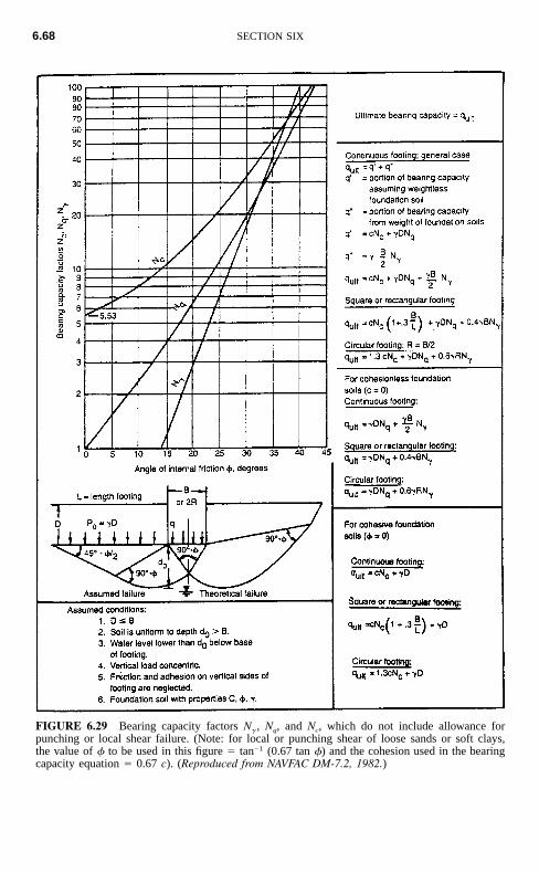
6.68 SECTION SIX
FIGURE 6.29 Bearing capacity factors N� , Nq, and Nc, which do not include allowance forpunching or local shear failure. (Note: for local or punching shear of loose sands or soft clays,the value of � to be used in this figure � tan (0.67 tan �) and the cohesion used in the bearing�1
capacity equation � 0.67 c). (Reproduced from NAVFAC DM-7.2, 1982.)
SOIL MECHANICS AND FOUNDATIONS 6.69
e � eccentricity of the load Q ; i.e., the lateral distance from Q to the centerof gravity of the footing
B � width of the footing
A usual requirement is that the load (Q ) must be located within the middle 1⁄3of the footing. The above equations are only valid for this condition. The value ofq � must not exceed the allowable bearing pressure (qall).
For dense or stiff soils, allowable bearing values in Table 6.14 are generallyconservative. For very loose or very soft soils, the allowable bearing values in Table6.14 may be too high.
6.6.2 Bearing Capacity for Deep Foundations in Granular Soil
Deep foundations are used when the upper soil stratum is too soft, weak, or com-pressible to support the foundation loads. Deep foundations are also used whenthere is a possibility of the undermining of the foundation. For example, bridgepiers are often founded on deep foundations to prevent a loss of support due toflood conditions which could cause river bottom scour. The most common types ofdeep foundations are piles and piers that support individual footings or mat foun-dations (Table 6.2). Piles are defined as relatively long, slender, column-like mem-bers often made of steel, concrete, or wood that are either driven into place or cast-in-place in predrilled holes. Common types of piles are as follows:
Batter Pile. A pile driven in at an angle inclined to the vertical to provide highresistance to lateral loads.End-Bearing Pile. A pile whose support capacity is derived principally fromthe resistance of the foundation material on which the pile tip rests. End-bearingpiles are often used when a soft upper layer is underlain by a dense or hardstratum. If the upper soft layer should settle, the pile could be subjected to down-drag forces, and the pile must be designed to resist these soil-induced forces.Friction Pile. A pile whose support capacity is derived principally from theresistance of the soil friction and/or adhesion mobilized along the side of thepile. Friction piles are often used in soft clays where the end-bearing resistanceis small because of punching shear at the pile tip.Combined End-Bearing and Friction Pile. A pile that derives its support ca-pacity from combined end-bearing resistance developed at the pile tip and fric-tional and/or adhesion resistance on the pile perimeter.
A pier is defined as a deep foundation system, similar to a cast-in-place pile,that consists of a column-like reinforced concrete member. Piers are often of largeenough diameter to enable down-hole inspection. Piers are also commonly referredto as drilled shafts, bored piles, or drilled caissons.
Many other methods are available for forming deep foundation elements. Ex-amples include earth stabilization columns, such as (NAVFAC DM-7.2, 1982):
Mixed-in-Place Piles. A mixed-in-place soil-cement or soil-lime pile.Vibro-Replacement Stone Columns. Vibroflotation or other method is used tomake a cylindrical, vertical hole that is filled with compacted gravel or crushedrock.
6.70 SECTION SIX
Grouted Stone Columns. Similar to the above but includes filling voids withbentonite-cement or water-sand-bentonite cement mixtures.Concrete Vibro Columns. Similar to stone columns, but concrete is used insteadof gravel.
Several different items are used in the design and construction of piles, includ-ing:
Engineering Analysis. Based on the results of subsurface exploration and lab-oratory testing, the bearing capacity of the deep foundation can be calculated ina similar manner to the previous section on shallow foundations. This sectionwill describe the engineering analyses for deep foundations in granular and co-hesive soil.Field Load Tests. Prior to the construction of the foundation, a pile or piercould be load tested in the field to determine its carrying capacity. Because ofthe uncertainties in the design of piles based on engineering analyses, pile loadtests are common. The pile load test can often result in a more economicalfoundation than one based solely on engineering analyses.Application of Pile Driving Resistance. Often the pile driving resistance (i.e.,blows per ft) is recorded as the pile is driven into place. When the anticipatedbearing layer is encountered, the driving resistance (blows per ft) should sub-stantially increase.Specifications and Experience. Other factors that should be considered in thedeep foundation design include governing building code or agency requirementsand local experience.
End Bearing Pile for Granular Soil. For an end bearing pile or pier, the bearingcapacity equation can be used to determine the ultimate bearing capacity (qult).When we compare the second and third term in Eq. (6.24), the value of B (widthof pile) is much less than the embedment depth (Dƒ ) of the pile. Therefore, thesecond term in Eq. (6.24) can be neglected. Assuming granular soil (c � 0), Eq.(6.24) reduces to the following:
Qpq � � � D N � �N (6.26)ult t ƒ q v qarea
where qult � the ultimate bearing capacity of the end-bearing pile or pierQp � point resistance force
area � pile tip area (B2 in the case of a square pile and �R 2 in the case ofa round pile)
��v vertical effective stress at the pile tipNq � dimensionless bearing capacity factor
For drilled piers or piles placed in predrilled holes, the value of Nq can beobtained from Fig. 6.28 or 6.29 based on the friction angle (�) of the granular soillocated at the pile tip. However, for driven piles, the values of Nq listed in Figs.6.28 and 6.29 are generally too conservative. Figure 6.30 presents a chart thatprovides the bearing capacity factor Nq from several different sources. Note in Fig.6.30 that at � � 30�, Nq varies from about 30 to 150, while at � � 40�, Nq variesfrom about 100 to 1000. This is a tremendous variation in Nq values and is relatedto the different approaches used by the various researchers, where in some cases
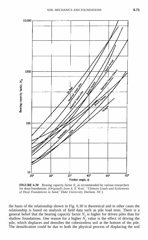
SOIL MECHANICS AND FOUNDATIONS 6.71
FIGURE 6.30 Bearing capacity factor Nq as recommended by various researchersfor deep foundations. (Originally from A. S. Vesic, ‘‘Ultimate Loads and Settlementsof Deep Foundations in Sand,’’ Duke University, Durham, NC.)
the basis of the relationship shown in Fig. 6.30 is theoretical and in other cases therelationship is based on analysis of field data such as pile load tests. There is ageneral belief that the bearing capacity factor Nq is higher for driven piles than forshallow foundations. One reason for a higher Nq value is the effect of driving thepile, which displaces and densifies the cohesionless soil at the bottom of the pile.The densification could be due to both the physical process of displacing the soil
6.72 SECTION SIX
and the driving vibrations. These actions would tend to increase the friction angleof the granular soil in the vicinity of the driven pile. Large-diameter piles wouldtend to displace and densify more soil than smaller-diameter piles.
Friction Pile for Granular Soil. As the name implies, a friction pile develops itsload carrying capacity due to the frictional resistance between the granular soil andthe pile perimeter. Piles subjected to vertical uplift forces would be designed asfriction piles because there would be no end-bearing resistance as the pile is pulledfrom the ground.
Based on a linear increase in frictional resistance with confining pressure, theaverage ultimate frictional capacity (qult) can be calculated as follows:
Qsq � � � tan � � � k tan � (6.27)ult h w v wsurface area
where qult � the average ultimate frictional capacity for the pile or pierQs � ultimate skin friction resistance force
Surface area � perimeter surface area of the pile, which is equal to 4DL for asquare pile and �DL for a round pile (D � diameter or width ofpile and L � length of pile)
��h average horizontal effective stress over the length of the pile or pier ��v average vertical effective stress over the length of the pile or pier
k � dimensionless parameter equal to divided by (because of the� �h vdensification of the granular soil associated with driven displace-ment piles, values of k between 1 and 2 are often assumed)
�w � friction angle between the cohesionless soil and the perimeter ofthe pile or pier (degrees)
Commonly used friction angles are �w � 3⁄4� for wood and concrete piles and�w � 20� for steel piles.
In Eq. (6.27), the term tan �w equals the shear strength (ƒ) between the pile�hor pier surface and the granular soil. This term is identical to Eq. (6.9) (with c � �0), that is, ƒ � tan ��. Thus, the frictional resistance force (Qs) in Eq. (6.27)�nis equal to the perimeter surface area times the shear strength of the soil at the pileor pier surface.
Combined End-Bearing and Friction Pile in Granular Soil. Piles and piers sub-jected to vertical compressive loads and embedded in a deposit of granular soil areusually treated in the design analysis as combined end-bearing and friction piles orpiers. This is because the pile or pier can develop substantial load-carrying capacityfrom both end-bearing and frictional resistance. To calculate the ultimate pile orpier capacity for a condition of combined end-bearing and friction, the value of Qp
from Eq. (6.26) is added to the value of Qs from Eq. (6.27). Usually the ultimatecapacity is divided by a factor of safety of 3 in order to calculate the allowablepile or pier load.
Pile Groups in Granular Soil. The previous discussion dealt with the load ca-pacity of a single pile in cohesionless soil. Usually pile groups are used to supportthe foundation elements, such as a group of piles supporting a pile cap or a matslab. In loose sand and gravel deposits, the load-carrying capacity of each pile inthe group may be greater than that of a single pile because of the densificationeffect due to driving the piles. Because of this densification effect, the load capacity
SOIL MECHANICS AND FOUNDATIONS 6.73
of the group is often taken as the load capacity of a single pile times the numberof piles in the group. An exception would be a situation where a weak layer un-derlies the cohesionless soil. In this case, group action of the piles could causethem to punch through the granular soil and into the weaker layer or cause excessivesettlement of the weak layer located below the pile tips.
In order to determine the settlement of the strata underlying the pile group, the2:1 approximation (see Art. 6.4.2) can be used to determine the increase in verticalstress (�v) for those soil layers located below the pile tip. If the piles in the groupare principally end-bearing, then the 2:1 approximation starts at the tip of the piles(L � bottom length of the pile group, B � width of the pile group, and z � depthbelow the tip of the piles, see Eq. 6.16). If the pile group develops its load-carryingcapacity principally through side friction, then the 2:1 approximation starts at adepth of 2⁄3D, where D � depth of the pile group.
6.6.3 Bearing Capacity for Deep Foundations in Cohesive Soil
The load-carrying capacity of piles and piers in cohesive soil is more complex thanthe analysis for granular soil. Some of the factors that may need to be consideredin the analysis are as follows (AASHTO, ‘‘Standard Specifications for Bridges,’’16th ed., American Association of State Highway and Transportation Officials,Washington, DC):
• A lower load-carrying capacity of a pile in a pile group as compared to that ofa single pile.
• The settlement of the underlying cohesive soil due to the load of the pile group.
• The effects of driving piles on adjacent structures or slopes. The ground willoften heave around piles driven into soft and saturated cohesive soil.
• The increase in load on the pile due to negative skin friction (i.e., down-dragloads) from consolidating soil.
• The effects of uplift loads from expansive and swelling clays.
• The reduction in shear strength of the cohesive soil due to construction tech-niques, such as the disturbance of sensitive clays or development of excess porewater pressures during the driving of the pile. There is often an increase in load-carrying capacity of a pile after it has been driven into a soft and saturated claydeposit. This increase with time is known as freeze or setup and is caused pri-marily by the dissipation of excess pore water pressures.
• The influence of fluctuations in the elevation of the groundwater table on theload-carrying capacity when analyzed in terms of effective stresses.
Total Stress Analysis. The ultimate load capacity of a single pile or pier in co-hesive soil is often determined by performing a total stress analysis. This is becausethe critical load on the pile, such as from wind or earthquake loads, is a short-termloading condition and thus the undrained shear strength of the cohesive soil willgovern. The total stress analysis for a single pile or pier in cohesive soil typicallyis based on the undrained shear strength (su � c) of the cohesive soil.
The ultimate load capacity of the pile or pier in cohesive soil would equal thesum of the ultimate end-bearing and ultimate side adhesion components. Using theTerzaghi bearing capacity equation (Eq. 6.24), the ultimate load capacity (Qult) ofa single pile or pier in cohesive soil equals:
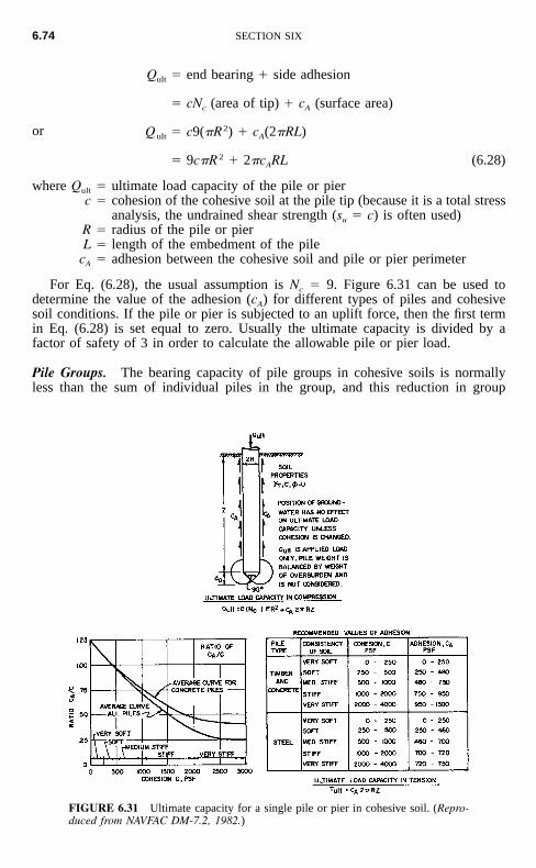
6.74 SECTION SIX
FIGURE 6.31 Ultimate capacity for a single pile or pier in cohesive soil. (Repro-duced from NAVFAC DM-7.2, 1982.)
Q � end bearing � side adhesionult
� cN (area of tip) � c (surface area)c A
2Q � c9(�R ) � c (2�RL)ult A
2� 9c�R � 2�c RL (6.28)A
or
where Qult � ultimate load capacity of the pile or pierc � cohesion of the cohesive soil at the pile tip (because it is a total stress
analysis, the undrained shear strength (su � c) is often used)R � radius of the pile or pierL � length of the embedment of the pile
cA � adhesion between the cohesive soil and pile or pier perimeter
For Eq. (6.28), the usual assumption is Nc � 9. Figure 6.31 can be used todetermine the value of the adhesion (cA) for different types of piles and cohesivesoil conditions. If the pile or pier is subjected to an uplift force, then the first termin Eq. (6.28) is set equal to zero. Usually the ultimate capacity is divided by afactor of safety of 3 in order to calculate the allowable pile or pier load.
Pile Groups. The bearing capacity of pile groups in cohesive soils is normallyless than the sum of individual piles in the group, and this reduction in group
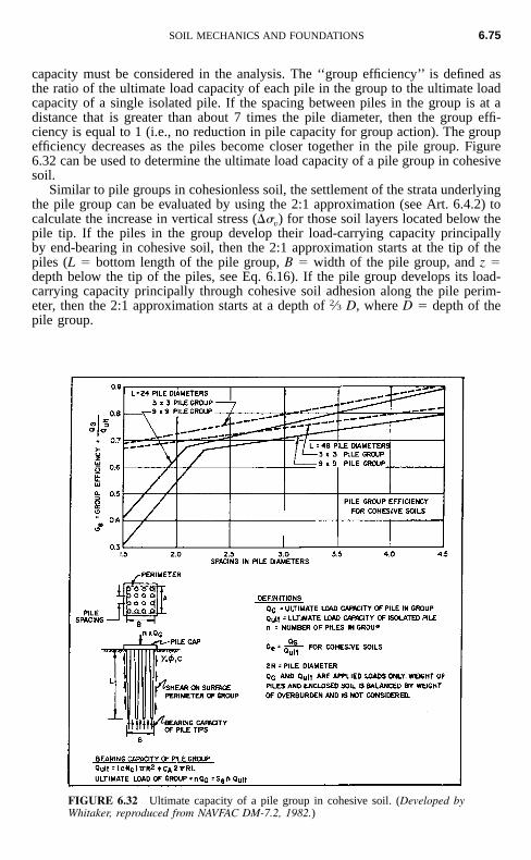
SOIL MECHANICS AND FOUNDATIONS 6.75
FIGURE 6.32 Ultimate capacity of a pile group in cohesive soil. (Developed byWhitaker, reproduced from NAVFAC DM-7.2, 1982.)
capacity must be considered in the analysis. The ‘‘group efficiency’’ is defined asthe ratio of the ultimate load capacity of each pile in the group to the ultimate loadcapacity of a single isolated pile. If the spacing between piles in the group is at adistance that is greater than about 7 times the pile diameter, then the group effi-ciency is equal to 1 (i.e., no reduction in pile capacity for group action). The groupefficiency decreases as the piles become closer together in the pile group. Figure6.32 can be used to determine the ultimate load capacity of a pile group in cohesivesoil.
Similar to pile groups in cohesionless soil, the settlement of the strata underlyingthe pile group can be evaluated by using the 2:1 approximation (see Art. 6.4.2) tocalculate the increase in vertical stress (�v) for those soil layers located below thepile tip. If the piles in the group develop their load-carrying capacity principallyby end-bearing in cohesive soil, then the 2:1 approximation starts at the tip of thepiles (L � bottom length of the pile group, B � width of the pile group, and z �depth below the tip of the piles, see Eq. 6.16). If the pile group develops its load-carrying capacity principally through cohesive soil adhesion along the pile perim-eter, then the 2:1 approximation starts at a depth of 2⁄3 D, where D � depth of thepile group.
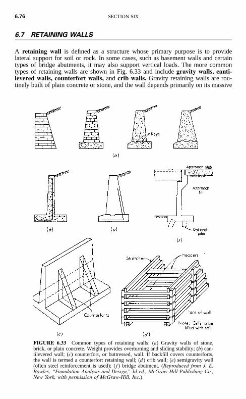
6.76 SECTION SIX
FIGURE 6.33 Common types of retaining walls: (a) Gravity walls of stone,brick, or plain concrete. Weight provides overturning and sliding stability; (b) can-tilevered wall; (c) counterfort, or buttressed, wall. If backfill covers counterforts,the wall is termed a counterfort retaining wall; (d ) crib wall; (e) semigravity wall(often steel reinforcement is used); ( f ) bridge abutment. (Reproduced from J. E.Bowles, ‘‘Foundation Analysis and Design,’’ 3d ed., McGraw-Hill Publishing Co.,New York, with permission of McGraw-Hill, Inc.)
6.7 RETAINING WALLS
A retaining wall is defined as a structure whose primary purpose is to providelateral support for soil or rock. In some cases, such as basement walls and certaintypes of bridge abutments, it may also support vertical loads. The more commontypes of retaining walls are shown in Fig. 6.33 and include gravity walls, canti-levered walls, counterfort walls, and crib walls. Gravity retaining walls are rou-tinely built of plain concrete or stone, and the wall depends primarily on its massive
SOIL MECHANICS AND FOUNDATIONS 6.77
weight to resist failure from overturning and sliding. Counterfort walls consist ofa footing, a wall stem, and intermittent vertical ribs (called counterforts) that tiethe footing and wall stem together. Crib walls consist of interlocking concrete mem-bers that form cells which are then filled with compacted soil.
Granular soils (sands or gravels) are the standard recommendation for backfillmaterial. There are several reasons for this recommendation:
1. Predictable Behavior. Import granular backfill generally has a more predictablebehavior in terms of earth pressure exerted on the wall. If silts or clays are usedas backfill material, expansive soil-related forces could be generated by thesesoil types.
2. Drainage System. To prevent the build-up of hydrostatic water pressure on theretaining wall, a drainage system is often constructed at the heel of the wall.This system will be more effective if highly permeable granular soil is used asbackfill.
3. Frost Action. In cold climates, the formation of ice lenses in the backfill soilcan cause so much lateral movement that the retaining wall will become un-usable. Backfill soil consisting of granular soil and the installation of a drainagesystem at the heel of the wall will help to protect the wall from frost action.
6.7.1 Retaining Wall Analyses
Figure 6.34 shows various types of retaining walls and the soil pressures acting onthe walls. Three types of soil pressures act on a retaining wall: (1) active earthpressure, which is exerted on the back side of the wall, (2) passive earth pressure,which acts on the front of the retaining wall footing, and (3) bearing pressure,which acts on the bottom of the retaining wall footing. These three pressures areindividually discussed below.
Active Earth Pressure. In order to calculate the active earth pressure resultantforce (PA), in kN per linear meter of wall or pounds per linear foot of wall, thefollowing equation is used for granular backfill:
21P � ⁄2k � H (6.29)A A t
where kA � active earth pressure coefficient�t � total unit weight of the granular backfillH � height over which the active earth pressure acts as defined in Fig. 6.34a
In its simplest form, the active earth pressure coefficient (kA) is equal to:
2 1k � tan (45� � ⁄2�) (6.30)A
where � � friction angle of the granular backfill. Equation (6.30) is known as theactive Rankine state, after the British engineer Rankine, who in 1857 obtained thisrelationship. Equation (6.30) is valid only for the simple case of a retaining wallthat has a vertical rear face, no friction between the rear wall face and backfill soil,and the backfill ground surface is horizontal. For retaining walls that do not meetthese requirements, the active earth pressure coefficient (kA) for Eq. (6.29) is oftendetermined using the Coulomb equation (see Fig. 6.35). Often the wall friction isneglected (� � 0�), but if it is included in the analysis, typical values are � � 3⁄4�
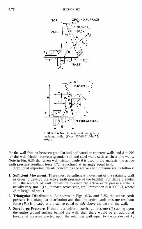
6.78 SECTION SIX
FIGURE 6.34a Gravity and semigravityretaining walls. (From NAVFAC DM-7.2,1982.)
for the wall friction between granular soil and wood or concrete walls and � � 20�for the wall friction between granular soil and steel walls such as sheet-pile walls.Note in Fig. 6.35 that when wall friction angle � is used in the analysis, the activeearth pressure resultant force (PA) is inclined at an angle equal to �.
Additional important details concerning the active earth pressure are as follows:
1. Sufficient Movement. There must be sufficient movement of the retaining wallin order to develop the active earth pressure of the backfill. For dense granularsoil, the amount of wall translation to reach the active earth pressure state isusually very small (i.e., to reach active state, wall translation � 0.0005 H, whereH � height of wall).
2. Triangular Distribution. As shown in Figs. 6.34 and 6.35, the active earthpressure is a triangular distribution and thus the active earth pressure resultantforce (PA) is located at a distance equal to 1⁄3H above the base of the wall.
3. Surcharge Pressure. If there is a uniform surcharge pressure (Q ) acting uponthe entire ground surface behind the wall, then there would be an additionalhorizontal pressure exerted upon the retaining wall equal to the product of kA
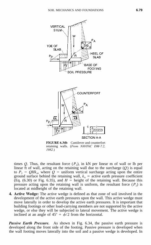
SOIL MECHANICS AND FOUNDATIONS 6.79
FIGURE 6.34b Cantilever and counterfortretaining walls. (From NAVFAC DM-7.2,1982.)
times Q. Thus, the resultant force (P2), in kN per linear m of wall or lb perlinear ft of wall, acting on the retaining wall due to the surcharge (Q ) is equalto P2 � QHkA, where Q � uniform vertical surcharge acting upon the entireground surface behind the retaining wall, kA � active earth pressure coefficient(Eq. (6.30) or Fig. 6.35), and H � height of the retaining wall. Because thispressure acting upon the retaining wall is uniform, the resultant force (P2) islocated at midheight of the retaining wall.
4. Active Wedge: The active wedge is defined as that zone of soil involved in thedevelopment of the active earth pressures upon the wall. This active wedge mustmove laterally in order to develop the active earth pressures. It is important thatbuilding footings or other load-carrying members are not supported by the activewedge, or else they will be subjected to lateral movement. The active wedge isinclined at an angle of 45� � � /2 from the horizontal.
Passive Earth Pressure. As shown in Fig. 6.34, the passive earth pressure isdeveloped along the front side of the footing. Passive pressure is developed whenthe wall footing moves laterally into the soil and a passive wedge is developed. In
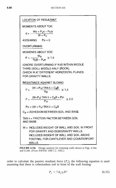
6.80 SECTION SIX
FIGURE 6.34c Design analysis for retaining walls shown in Figs. 6.34aand 6.34b. (From NAVFAC DM-7.2, 1982.)
order to calculate the passive resultant force (Pp), the following equation is usedassuming that there is cohesionless soil in front of the wall footing:
21P � ⁄2k � D (6.31)p p t
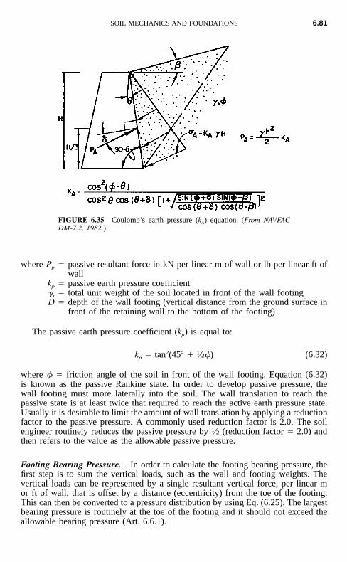
SOIL MECHANICS AND FOUNDATIONS 6.81
FIGURE 6.35 Coulomb’s earth pressure (kA) equation. (From NAVFACDM-7.2, 1982.)
where Pp � passive resultant force in kN per linear m of wall or lb per linear ft ofwall
kp � passive earth pressure coefficient�t � total unit weight of the soil located in front of the wall footingD � depth of the wall footing (vertical distance from the ground surface in
front of the retaining wall to the bottom of the footing)
The passive earth pressure coefficient (kp) is equal to:
2 1k � tan (45� � ⁄2�) (6.32)p
where � � friction angle of the soil in front of the wall footing. Equation (6.32)is known as the passive Rankine state. In order to develop passive pressure, thewall footing must more laterally into the soil. The wall translation to reach thepassive state is at least twice that required to reach the active earth pressure state.Usually it is desirable to limit the amount of wall translation by applying a reductionfactor to the passive pressure. A commonly used reduction factor is 2.0. The soilengineer routinely reduces the passive pressure by 1⁄2 (reduction factor � 2.0) andthen refers to the value as the allowable passive pressure.
Footing Bearing Pressure. In order to calculate the footing bearing pressure, thefirst step is to sum the vertical loads, such as the wall and footing weights. Thevertical loads can be represented by a single resultant vertical force, per linear mor ft of wall, that is offset by a distance (eccentricity) from the toe of the footing.This can then be converted to a pressure distribution by using Eq. (6.25). The largestbearing pressure is routinely at the toe of the footing and it should not exceed theallowable bearing pressure (Art. 6.6.1).
6.82 SECTION SIX
Retaining Wall Analyses. Once the active earth pressure resultant force (PA) andthe passive resultant force (Pp) have been calculated, the design analysis is per-formed as indicated in Fig. 6.34c. The retaining wall analysis includes determiningthe resultant location of the forces (i.e., calculate d, which should be within themiddle third of the footing), the factor of safety for overturning, and the factor ofsafety for sliding. The adhesion (ca) between the bottom of the footing and theunderlying soil is often ignored for the sliding analysis.
6.7.2 Restrained Retaining Walls
As mentioned in the previous article, in order for the active wedge to be developed,there must be sufficient movement of the retaining wall. There are many caseswhere movement of the retaining wall is restricted. Examples include massivebridge abutments, rigid basement walls, and retaining walls that are anchored innonyielding rock. These cases are often described as restrained retaining walls.
In order to determine the earth pressure acting on a restrained retaining wall,Eq. (6.29) can be utilized where the coefficient of earth pressure at rest (k0) issubstituted for kA. A common value of k0 for granular soil that is used for restrainedretaining walls is 0.5. Restrained retaining walls are especially susceptible to higherearth pressures induced by heavy compaction equipment, and extra care must betaken during the compaction of backfill for restrained retaining walls.
6.7.3 Mechanically Stabilized Earth Retaining Walls
Mechanically stabilized earth retaining walls (also known as MSE retainingwalls) are typically composed of strip- or grid-type (geosynthetic) reinforcement.Because they are often more economical to construct than conventional concreteretaining walls, mechanically stabilized earth retaining walls have become verypopular in the past decade. A mechanically stabilized earth retaining wall is com-posed of three elements: (1) wall facing material, (2) soil reinforcement, such asstrip- or grid-type reinforcement, and (3) compacted fill between the soil reinforce-ment.
The design analysis for a mechanically stabilized earth retaining wall is morecomplex than for a cantilevered retaining wall. For a mechanically stabilized earthretaining wall, both the internal and external stability must be checked.
External Stability. The analysis for the external stability is similar to that for agravity retaining wall. For example, Figs. 6.36 and 6.37 present the design analysisfor external stability for a level backfill condition and a sloping backfill condition.In both Figs. 6.36 and 6.37, the zone of mechanically stabilized earth mass is treatedin a similar fashion as a massive gravity retaining wall. The following analysesmust be performed:
1. Allowable bearing pressure: the bearing pressure due to the reinforced soil massmust not exceed the allowable bearing pressure.
2. Factor of safety of sliding: the reinforced soil mass must have an adequate factorof safety for sliding.
3. Factor of safety of overturning; the reinforced soil mass must have an adequatefactor of safety for overturning about Point O.
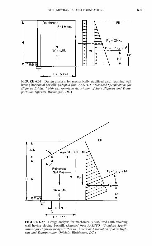
SOIL MECHANICS AND FOUNDATIONS 6.83
FIGURE 6.36 Design analysis for mechanically stabilized earth retaining wallhaving horizontal backfill. (Adapted from AASHTO, ‘‘Standard Specifications forHighway Bridges,’’ 16th ed., American Association of State Highway and Trans-portation Officials, Washington, DC.)
FIGURE 6.37 Design analysis for mechanically stabilized earth retainingwall having sloping backfill. (Adapted from AASHTO, ‘‘Standard Specifi-cations for Highway Bridges,’’ 16th ed., American Association of State High-way and Transportation Officials, Washington, DC.)
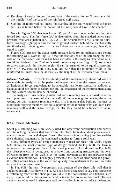
6.84 SECTION SIX
4. Resultant of vertical forces: the resultant of the vertical forces N must be withinthe middle 1⁄3 of the base of the reinforced soil mass.
5. Stability of reinforced soil mass: the stability of the entire reinforced soil mass(i.e., shear failure below the bottom of the wall) would have to be checked.
Note in Figure 6.36 that two forces (P1 and P2) are shown acting on the rein-forced soil mass. The first force (P1) is determined from the standard active earthpressure resultant equation (i.e., Eq. 6.29). The second force (P2) is due to a uni-form surcharge (Q) applied to the entire ground surface behind the mechanicallystabilized earth retaining wall. If the wall does not have a surcharge, then P2 isequal to zero.
Figure 6.37 presents the active earth pressure force for an inclined slope behindthe retaining wall. Note in Fig. 6.37 that the friction (�) of the soil along the backside of the reinforced soil mass has been included in the analysis. The value of kA
would be obtained from Coulomb’s earth pressure equation (Fig. 6.35). As a con-servative approach, the friction angle (�) can be assumed to be equal to zero andthen PH � PA. Note in both Figs. 6.36 and 6.37 that the minimum width of thereinforced soil mass must be at least 7⁄10 the height of the reinforced soil mass.
Internal Stability. To check the stability of the mechanically stabilized zone, aslope stability analysis can be performed where the soil reinforcement is modeledas horizontal forces equivalent to its allowable tensile resistance. In addition tocalculation of the factor of safety, the pull-out resistance of the reinforcement alongthe slip surface should also be checked.
The analysis of mechanically stabilized earth retaining walls is based on activeearth pressures. It is assumed that the wall will move enough to develop the activewedge. As with concrete retaining walls, it is important that building footings orother load carrying members are not supported by the mechanically stabilized earthretaining wall and the active wedge, or else they could be subjected to lateralmovement.
6.7.4 Sheet Pile Walls
Sheet pile retaining walls are widely used for waterfront construction and consistof interlocking members that are driven into place. Individual sheet piles come inmany different sizes and shapes. Sheet piles have an interlocking joint that enablesthe individual segments to be connected together to form a solid wall.
Many different types of design methods are used for sheet pile walls. Figure6.38 shows the most common type of design method. In Fig. 6.38, the term Hrepresents the unsupported face of the sheet pile wall. As indicated in Fig. 6.38,this sheet pile wall is being used as a waterfront retaining structure and the levelof water in front of the wall is at the same elevation as the groundwater tableelevation behind the wall. For highly permeable soil, such as clean sand and gravel,this often occurs because the water can quickly flow underneath the wall in orderto equalize the water levels.
In Fig. 6.38, the term D represents that portion of the sheet pile wall that isanchored in soil. Also shown in Fig. 6.38 is a force designated as Ap. This representsa restraining force on the sheet pile wall due to the construction of a tieback, suchas by using a rod that has a grouted end or is attached to an anchor block. Tiebackanchors are often used in sheet pile wall construction in order to reduce the bending
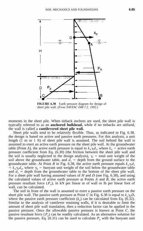
SOIL MECHANICS AND FOUNDATIONS 6.85
FIGURE 6.38 Earth pressure diagram for design ofsheet pile wall. (From NAVFAC DM-7.2, 1982.)
moments in the sheet pile. When tieback anchors are used, the sheet pile wall istypically referred to as an anchored bulkhead, while if no tiebacks are utilized,the wall is called a cantilevered sheet pile wall.
Sheet pile walls tend to be relatively flexible. Thus, as indicated in Fig. 6.38,the design is based on active and passive earth pressures. For this analysis, a unitlength (1 m or 1 ft) of sheet pile wall is assumed. The soil behind the wall isassumed to exert an active earth pressure on the sheet pile wall. At the groundwatertable (Point A), the active earth pressure is equal to kA�td1, where kA � active earthpressure coefficient from Eq. (6.30) (the friction between the sheet pile wall andthe soil is usually neglected in the design analysis), �t � total unit weight of thesoil above the groundwater table, and d1 � depth from the ground surface to thegroundwater table. At Point B in Fig. 6.38, the active earth pressure equals kA�td1
� kA�bd2, where �b � buoyant unit weight of the soil below the groundwater tableand d2 � depth from the groundwater table to the bottom of the sheet pile wall.For a sheet pile wall having assumed values of H and D (see Fig. 6.38), and usingthe calculated values of active earth pressure at Points A and B, the active earthpressure resultant force (PA), in kN per linear m of wall or lb per linear foot ofwall, can be calculated.
The soil in front of the wall is assumed to exert a passive earth pressure on thesheet pile wall. The passive earth pressure at Point C in Fig. 6.38 is equal to kp�bD,where the passive earth pressure coefficient (kp) can be calculated from Eq. (6.32).Similar to the analysis of cantilever retaining walls, if it is desirable to limit theamount of sheet pile wall translation, then a reduction factor can be applied to thepassive pressure. Once the allowable passive pressure is known at Point C, thepassive resultant force (Pp) can be readily calculated. As an alternative solution forthe passive pressure, Eq. (6.31) can be used to calculate Pp with the buoyant unit
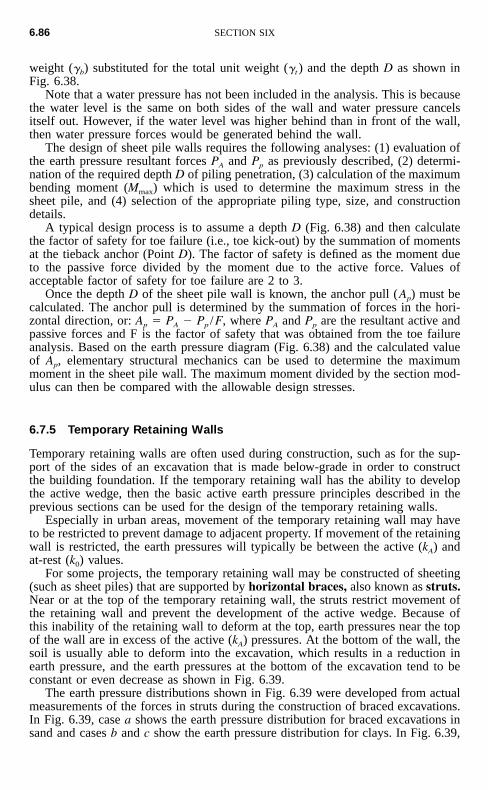
6.86 SECTION SIX
weight (�b) substituted for the total unit weight (�t ) and the depth D as shown inFig. 6.38.
Note that a water pressure has not been included in the analysis. This is becausethe water level is the same on both sides of the wall and water pressure cancelsitself out. However, if the water level was higher behind than in front of the wall,then water pressure forces would be generated behind the wall.
The design of sheet pile walls requires the following analyses: (1) evaluation ofthe earth pressure resultant forces PA and Pp as previously described, (2) determi-nation of the required depth D of piling penetration, (3) calculation of the maximumbending moment (Mmax) which is used to determine the maximum stress in thesheet pile, and (4) selection of the appropriate piling type, size, and constructiondetails.
A typical design process is to assume a depth D (Fig. 6.38) and then calculatethe factor of safety for toe failure (i.e., toe kick-out) by the summation of momentsat the tieback anchor (Point D). The factor of safety is defined as the moment dueto the passive force divided by the moment due to the active force. Values ofacceptable factor of safety for toe failure are 2 to 3.
Once the depth D of the sheet pile wall is known, the anchor pull (Ap) must becalculated. The anchor pull is determined by the summation of forces in the hori-zontal direction, or: Ap � PA � Pp /F, where PA and Pp are the resultant active andpassive forces and F is the factor of safety that was obtained from the toe failureanalysis. Based on the earth pressure diagram (Fig. 6.38) and the calculated valueof Ap, elementary structural mechanics can be used to determine the maximummoment in the sheet pile wall. The maximum moment divided by the section mod-ulus can then be compared with the allowable design stresses.
6.7.5 Temporary Retaining Walls
Temporary retaining walls are often used during construction, such as for the sup-port of the sides of an excavation that is made below-grade in order to constructthe building foundation. If the temporary retaining wall has the ability to developthe active wedge, then the basic active earth pressure principles described in theprevious sections can be used for the design of the temporary retaining walls.
Especially in urban areas, movement of the temporary retaining wall may haveto be restricted to prevent damage to adjacent property. If movement of the retainingwall is restricted, the earth pressures will typically be between the active (kA) andat-rest (k0) values.
For some projects, the temporary retaining wall may be constructed of sheeting(such as sheet piles) that are supported by horizontal braces, also known as struts.Near or at the top of the temporary retaining wall, the struts restrict movement ofthe retaining wall and prevent the development of the active wedge. Because ofthis inability of the retaining wall to deform at the top, earth pressures near the topof the wall are in excess of the active (kA) pressures. At the bottom of the wall, thesoil is usually able to deform into the excavation, which results in a reduction inearth pressure, and the earth pressures at the bottom of the excavation tend to beconstant or even decrease as shown in Fig. 6.39.
The earth pressure distributions shown in Fig. 6.39 were developed from actualmeasurements of the forces in struts during the construction of braced excavations.In Fig. 6.39, case a shows the earth pressure distribution for braced excavations insand and cases b and c show the earth pressure distribution for clays. In Fig. 6.39,
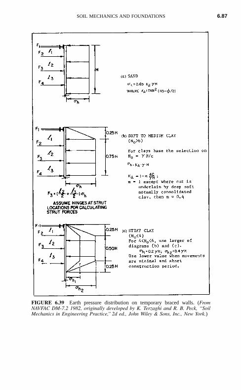
SOIL MECHANICS AND FOUNDATIONS 6.87
FIGURE 6.39 Earth pressure distribution on temporary braced walls. (FromNAVFAC DM-7.2 1982, originally developed by K. Terzaghi and R. B. Peck, ‘‘SoilMechanics in Engineering Practice,’’ 2d ed., John Wiley & Sons, Inc., New York.)
6.88 SECTION SIX
the distance H represents the depth of the excavation (i.e., the height of the exposedwall surface). The earth pressure distribution is applied over the exposed height (H)of the wall surface with the earth pressures transferred from the wall sheeting tothe struts (the struts are labeled with the forces F1, F2, etc.).
Any surcharge pressures, such as surcharge pressures on the ground surfaceadjacent the excavation, must be added to the pressure distributions shown in Fig.6.39. In addition, if the sand deposit has a groundwater table that is above the levelof the bottom of the excavation, then water pressures must be added to the case apressure distribution shown in Fig. 6.39.
Because the excavations are temporary (i.e., short-term condition), the undrainedshear strength (su � c) is used for the analysis of the earth pressure distributionsfor clay. The earth pressure distributions for clay (i.e., cases b and c) are not validfor permanent walls or for walls where the groundwater table is above the bottomof the excavation.
6.8 FOUNDATIONS
This section deals with the selection of the type of foundation. The selection of aparticular type of foundation is often based on a number of factors, such as:
1. Adequate Depth. It must have an adequate depth to prevent frost damage. Forsuch foundations as bridge piers, the depth of the foundation must be sufficientto prevent undermining by scour.
2. Bearing Capacity Failure. The foundation must be safe against a bearing ca-pacity failure (Art. 6.6).
3. Settlement. The foundation must not settle to such an extent that it damagesthe structure (Art. 6.5).
4. Quality. The foundation must be of adequate quality so that it is not subjectedto deterioration, such as the sulfate attack of concrete footings.
5. Adequate Strength. The foundation must be designed with sufficient strengththat it does not fracture or break apart under the applied superstructure loads. Itmust also be properly constructed in conformance with the design specifications.
6. Adverse Soil Changes. The foundation must be able to resist long-term adversesoil changes. An example is expansive soil (silts and clays), which could expandor shrink causing movement of the foundation and damage to the structure.
7. Seismic Forces. The foundation must be able to support the structure during anearthquake without excessive settlement or lateral movement.
6.8.1 Shallow Foundations
A shallow foundation is often selected when the structural load will not causeexcessive settlement of the underlying soil layers. In general, shallow foundationsare more economical to construct than deep foundations. Common types of shallowfoundations are listed in Table 6.2 and described below:
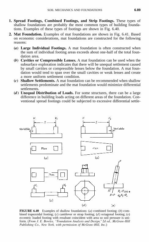
SOIL MECHANICS AND FOUNDATIONS 6.89
FIGURE 6.40 Examples of shallow foundations: (a) combined footing; (b) com-bined trapezoidal footing; (c) cantilever or strap footing; (d ) octagonal footing; (e)eccentric loaded footing with resultant coincident with area so soil pressure is uni-form. (From J. E. Bowles, ‘‘Foundation Analysis and Design,’’ 2d ed., McGraw-HillPublishing Co., New York, with permission of McGraw-Hill, Inc.)
1. Spread Footings, Combined Footings, and Strip Footings. These types ofshallow foundations are probably the most common types of building founda-tions. Examples of these types of footings are shown in Fig. 6.40.
2. Mat Foundation. Examples of mat foundations are shown in Fig. 6.41. Basedon economic considerations, mat foundations are constructed for the followingreasons:
(a) Large Individual Footings. A mat foundation is often constructed whenthe sum of individual footing areas exceeds about one-half of the total foun-dation area.
(b) Cavities or Compressible Lenses. A mat foundation can be used when thesubsurface exploration indicates that there will be unequal settlement causedby small cavities or compressible lenses below the foundation. A mat foun-dation would tend to span over the small cavities or weak lenses and createa more uniform settlement condition.
(c) Shallow Settlements. A mat foundation can be recommended when shallowsettlements predominate and the mat foundation would minimize differentialsettlements.
(d ) Unequal Distribution of Loads. For some structures, there can be a largedifference in building loads acting on different areas of the foundation. Con-ventional spread footings could be subjected to excessive differential settle-
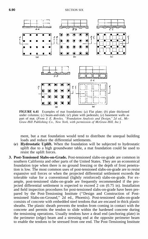
6.90 SECTION SIX
FIGURE 6.41 Examples of mat foundations: (a) Flat plate; (b) plate thickenedunder columns; (c) beam-and-slab; (d ) plate with pedestals; (e) basement walls aspart of mat. (From J. E. Bowles, ‘‘Foundation Analysis and Design,’’ 2d ed., Mc-Graw-Hill Publishing Co., New York, with permission of McGraw-Hill, Inc.)
ment, but a mat foundation would tend to distribute the unequal buildingloads and reduce the differential settlements.
(e) Hydrostatic Uplift. When the foundation will be subjected to hydrostaticuplift due to a high groundwater table, a mat foundation could be used toresist the uplift forces.
3. Post-Tensioned Slabs-on-Grade. Post-tensioned slabs-on-grade are common insouthern California and other parts of the United States. They are an economicalfoundation type when there is no ground freezing or the depth of frost penetra-tion is low. The most common uses of post-tensioned slabs-on-grade are to resistexpansive soil forces or when the projected differential settlement exceeds thetolerable value for a conventional (lightly reinforced) slabs-on-grade. For ex-ample, post-tensioned slabs-on-grade are frequently recommended if the pro-jected differential settlement is expected to exceed 2 cm (0.75 in). Installationand field inspection procedures for post-tensioned slabs-on-grade have been pre-pared by the Post-Tensioning Institute (‘‘Design and Construction of Post-tensioned Slabs-on-Ground,’’ 2d ed., Phoenix). Post-tensioned slabs-on-gradeconsists of concrete with embedded steel tendons that are encased in thick plasticsheaths. The plastic sheath prevents the tendon from coming in contact with theconcrete and permits the tendon to slide within the hardened concrete duringthe tensioning operations. Usually tendons have a dead end (anchoring plate) inthe perimeter (edge) beam and a stressing end at the opposite perimeter beamto enable the tendons to be stressed from one end. The Post-Tensioning Institute
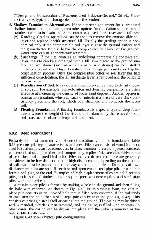
SOIL MECHANICS AND FOUNDATIONS 6.91
(‘‘Design and Construction of Post-tensioned Slabs-on-Ground,’’ 2d ed., Phoe-nix) provides typical anchorage details for the tendons.
4. Shallow Foundation Alternatives. If the expected settlement for a proposedshallow foundation is too large, then other options for foundation support or soilstabilization must be evaluated. Some commonly used alternatives are as follows:(a) Grading. Grading operations can be used to remove the compressible soil
layer and replace it with structural fill. Usually the grading option is eco-nomical only if the compressible soil layer is near the ground surface andthe groundwater table is below the compressible soil layer or the ground-water table can be economically lowered.
(b) Surcharge. If the site contains an underlying compressible cohesive soillayer, the site can be surcharged with a fill layer placed at the ground sur-face. Vertical drains (such as wick drains or sand drains) can be installedin the compressible soil layer to reduce the drainage paths and speed up theconsolidation process. Once the compressible cohesive soil layer has hadsufficient consolidation, the fill surcharge layer is removed and the buildingis constructed.
(c) Densification of Soil. Many different methods can be used to densify looseor soft soil. For example, vibro-flotation and dynamic compaction are ofteneffective at increasing the density of loose sand deposits. Another option iscompaction grouting, which consists of intruding a mass of very thick con-sistency grout into the soil, which both displaces and compacts the loosesoil.
(d ) Floating Foundation. A floating foundation is a special type of deep foun-dation where the weight of the structure is balanced by the removal of soiland construction of an underground basement.
6.8.2 Deep Foundations
Probably the most common type of deep foundation is the pile foundation. Table6.15 presents pile type characteristics and uses. Piles can consist of wood (timber),steel H-sections, precast concrete, cast-in-place concrete, pressure injected concrete,concrete filled steel pipe piles, and composite type piles. Piles are either driven intoplace or installed in predrilled holes. Piles that are driven into place are generallyconsidered to be low displacement or high displacement, depending on the amountof soil that must be pushed out of the way as the pile is driven. Examples of low-displacement piles are steel H-sections and open-ended steel pipe piles that do notform a soil plug at the end. Examples of high-displacement piles are solid sectionpiles, such as round timber piles or square precast concrete piles, and steel pipepiles with a closed end.
A cast-in-place pile is formed by making a hole in the ground and then fillingthe hole with concrete. As shown in Fig. 6.42, in its simplest form, the cast-in-place pile consists of an uncased hole that is filled with concrete. If the soil tendsto cave into the hole, then a shell-type pile can be installed (see Fig. 6.42). Thisconsists of driving a steel shell or casing into the ground. The casing may be drivenwith a mandrel, which is then removed, and the casing is filled with concrete. Inother cases, the casing can be driven into place and then slowly removed as thehole is filled with concrete.
Figure 6.43 shows typical pile configurations.
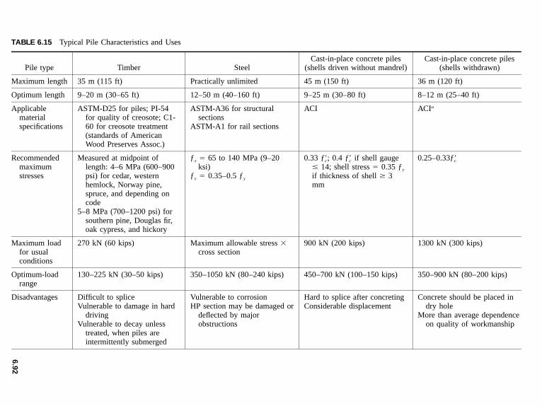
6.9
2
TABLE 6.15 Typical Pile Characteristics and Uses
Pile type Timber SteelCast-in-place concrete piles
(shells driven without mandrel)Cast-in-place concrete piles
(shells withdrawn)
Maximum length 35 m (115 ft) Practically unlimited 45 m (150 ft) 36 m (120 ft)
Optimum length 9–20 m (30–65 ft) 12–50 m (40–160 ft) 9–25 m (30–80 ft) 8–12 m (25–40 ft)
Applicablematerialspecifications
ASTM-D25 for piles; PI-54for quality of creosote; C1-60 for creosote treatment(standards of AmericanWood Preserves Assoc.)
ASTM-A36 for structuralsections
ASTM-A1 for rail sections
ACI ACIa
Recommendedmaximumstresses
Measured at midpoint oflength: 4–6 MPa (600–900psi) for cedar, westernhemlock, Norway pine,spruce, and depending oncode
5–8 MPa (700–1200 psi) forsouthern pine, Douglas fir,oak cypress, and hickory
ƒs � 65 to 140 MPa (9–20ksi)
ƒs � 0.35–0.5 ƒy
0.33 ; 0.4 if shell gaugeƒ� ƒ�c c
� 14; shell stress � 0.35 ƒy
if thickness of shell � 3mm
0.25–0.33ƒ�c
Maximum loadfor usualconditions
270 kN (60 kips) Maximum allowable stress �cross section
900 kN (200 kips) 1300 kN (300 kips)
Optimum-loadrange
130–225 kN (30–50 kips) 350–1050 kN (80–240 kips) 450–700 kN (100–150 kips) 350–900 kN (80–200 kips)
Disadvantages Difficult to spliceVulnerable to damage in hard
drivingVulnerable to decay unless
treated, when piles areintermittently submerged
Vulnerable to corrosionHP section may be damaged or
deflected by majorobstructions
Hard to splice after concretingConsiderable displacement
Concrete should be placed indry hole
More than average dependenceon quality of workmanship
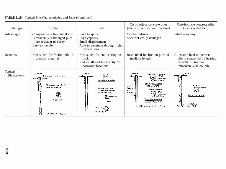
6.9
3
TABLE 6.15 Typical Pile Characteristics and Uses (Continued)
Pile type Timber SteelCast-in-place concrete piles
(shells driven without mandrel)Cast-in-place concrete piles
(shells withdrawn)
Advantages Comparatively low initial costPermanently submerged piles
are resistant to decayEasy to handle
Easy to spliceHigh capacitySmall displacementAble to penetrate through light
obstructions
Can be redrivenShell not easily damaged
Initial economy
Remarks Best suited for friction pile ingranular material
Best suited for end bearing onrock
Reduce allowable capacity forcorrosive locations
Best suited for friction piles ofmedium length
Allowable load on pedestalpile is controlled by bearingcapacity of stratumimmediately below pile
Typicalillustrations
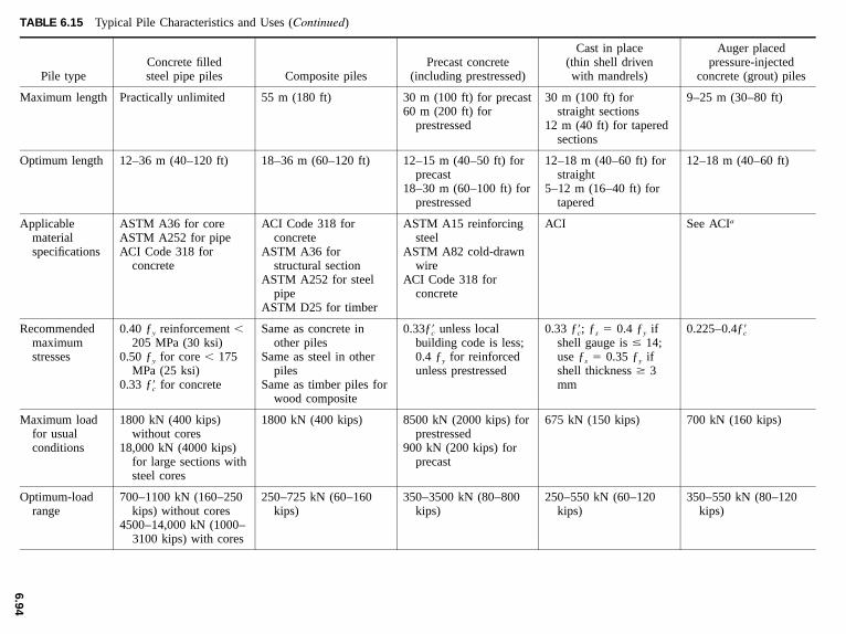
6.9
4
TABLE 6.15 Typical Pile Characteristics and Uses (Continued)
Pile typeConcrete filledsteel pipe piles Composite piles
Precast concrete(including prestressed)
Cast in place(thin shell drivenwith mandrels)
Auger placedpressure-injected
concrete (grout) piles
Maximum length Practically unlimited 55 m (180 ft) 30 m (100 ft) for precast60 m (200 ft) for
prestressed
30 m (100 ft) forstraight sections
12 m (40 ft) for taperedsections
9–25 m (30–80 ft)
Optimum length 12–36 m (40–120 ft) 18–36 m (60–120 ft) 12–15 m (40–50 ft) forprecast
18–30 m (60–100 ft) forprestressed
12–18 m (40–60 ft) forstraight
5–12 m (16–40 ft) fortapered
12–18 m (40–60 ft)
Applicablematerialspecifications
ASTM A36 for coreASTM A252 for pipeACI Code 318 for
concrete
ACI Code 318 forconcrete
ASTM A36 forstructural section
ASTM A252 for steelpipe
ASTM D25 for timber
ASTM A15 reinforcingsteel
ASTM A82 cold-drawnwire
ACI Code 318 forconcrete
ACI See ACIa
Recommendedmaximumstresses
0.40 ƒy reinforcement �205 MPa (30 ksi)
0.50 ƒy for core � 175MPa (25 ksi)
0.33 for concreteƒ�c
Same as concrete inother piles
Same as steel in otherpiles
Same as timber piles forwood composite
0.33 unless localƒ�cbuilding code is less;0.4 ƒy for reinforcedunless prestressed
0.33 ; ƒs � 0.4 ƒy ifƒ�cshell gauge is � 14;use ƒs � 0.35 ƒy ifshell thickness � 3mm
0.225–0.4ƒ�c
Maximum loadfor usualconditions
1800 kN (400 kips)without cores
18,000 kN (4000 kips)for large sections withsteel cores
1800 kN (400 kips) 8500 kN (2000 kips) forprestressed
900 kN (200 kips) forprecast
675 kN (150 kips) 700 kN (160 kips)
Optimum-loadrange
700–1100 kN (160–250kips) without cores
4500–14,000 kN (1000–3100 kips) with cores
250–725 kN (60–160kips)
350–3500 kN (80–800kips)
250–550 kN (60–120kips)
350–550 kN (80–120kips)
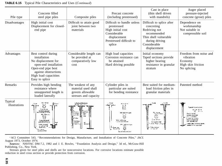
6.9
5
TABLE 6.15 Typical Pile Characteristics and Uses (Continued)
Pile typeConcrete filledsteel pipe piles Composite piles
Precast concrete(including prestressed)
Cast in place(thin shell drivenwith mandrels)
Auger placedpressure-injected
concrete (grout) piles
Disadvantages High initial costDisplacement for closed-
end pipe
Difficult to attain goodjoint between twomaterials
Difficult to handle unlessprestressed
High initial costConsiderable
displacementPrestressed difficult to
splice
Difficult to splice afterconcreting
Redriving notrecommended
Thin shell vulnerableduring driving
Considerabledisplacement
Dependence onworkmanship
Not suitable incompressible soil
Advantages Best control duringinstallation
No displacement foropen-end installation
Open-end pipe bestagainst obstructions
High load capacititesEasy to splice
Considerable length canbe provided atcomparatively lowcost
High load capacitiesCorrosion resistance can
be attainedHard driving possible
Initial economyTaped sections provide
higher bearingresistance in granularstratum
Freedom from noise andvibration
EconomyHigh skin frictionNo splicing
Remarks Provides high bendingresistance whereunsupported length isloaded laterally
The weakest of anymaterial used shallgovern allowablestresses and capacity
Cylinder piles inparticular are suitedfor bending resistance
Best suited for medium-load friction piles ingranular materials
Patented method
Typicalillustrations
a ACI Committee 543, ‘‘Recommendations for Design, Manufacture, and Installation of Concrete Piles,’’ JACI,August 1973, October 1974.
Sources: NAVFAC DM-7.2, 1982 and J. E. Bowles, ‘‘Foundation Analysis and Design,’’ 3d ed., McGraw-HillPublishing, Co., New York.
Stresses given for steel piles and shells are for noncorrosive locations. For corrosive locations estimate possiblereduction in steel cross section or provide protection from corrosion.
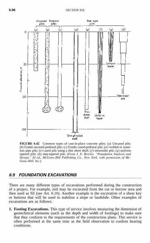
6.96 SECTION SIX
FIGURE 6.42 Common types of cast-in-place concrete piles: (a) Uncased pile;(b) Franki uncased-pedestal pile; (c) Franki cased-pedestal pile; (d ) welded or seam-less pipe pile; (e) cased pile using a thin sheet shell; ( f ) monotube pile; (g) uniformtapered pile; (h) step-tapered pile. (From J. E. Bowles, ‘‘Foundation Analysis andDesign,’’ 3d ed., McGraw-Hill Publishing Co., New York, with permission of Mc-Graw-Hill, Inc.)
6.9 FOUNDATION EXCAVATIONS
There are many different types of excavations performed during the constructionof a project. For example, soil may be excavated from the cut or borrow area andthen used as fill (see Art. 6.10). Another example is the excavation of a shear keyor buttress that will be used to stabilize a slope or landslide. Other examples ofexcavations are as follows:
1. Footing Excavations. This type of service involves measuring the dimension ofgeotechnical elements (such as the depth and width of footings) to make surethat they conform to the requirements of the construction plans. This service isoften performed at the same time as the field observation to confirm bearingconditions.
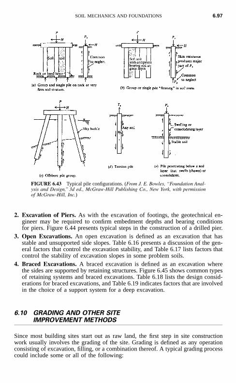
SOIL MECHANICS AND FOUNDATIONS 6.97
FIGURE 6.43 Typical pile configurations. (From J. E. Bowles, ‘‘Foundation Anal-ysis and Design,’’ 3d ed., McGraw-Hill Publishing Co., New York, with permissionof McGraw-Hill, Inc.)
2. Excavation of Piers. As with the excavation of footings, the geotechnical en-gineer may be required to confirm embedment depths and bearing conditionsfor piers. Figure 6.44 presents typical steps in the construction of a drilled pier.
3. Open Excavations. An open excavation is defined as an excavation that hasstable and unsupported side slopes. Table 6.16 presents a discussion of the gen-eral factors that control the excavation stability, and Table 6.17 lists factors thatcontrol the stability of excavation slopes in some problem soils.
4. Braced Excavations. A braced excavation is defined as an excavation wherethe sides are supported by retaining structures. Figure 6.45 shows common typesof retaining systems and braced excavations. Table 6.18 lists the design consid-erations for braced excavations, and Table 6.19 indicates factors that are involvedin the choice of a support system for a deep excavation.
6.10 GRADING AND OTHER SITEIMPROVEMENT METHODS
Since most building sites start out as raw land, the first step in site constructionwork usually involves the grading of the site. Grading is defined as any operationconsisting of excavation, filling, or a combination thereof. A typical grading processcould include some or all of the following:
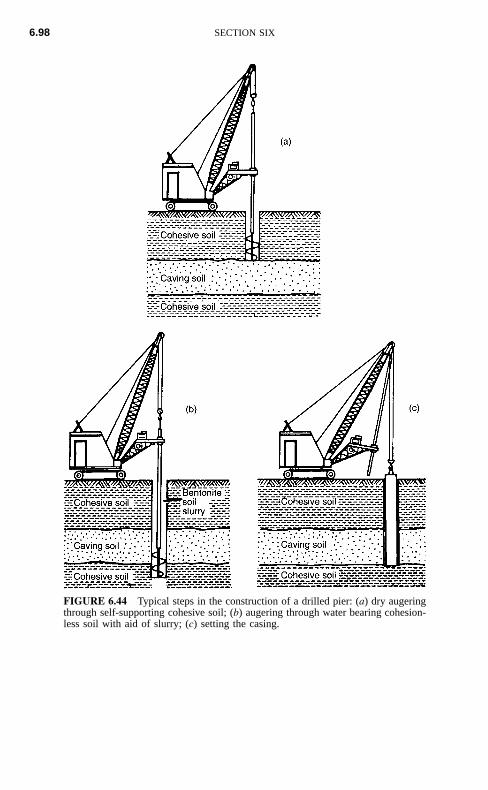
6.98 SECTION SIX
FIGURE 6.44 Typical steps in the construction of a drilled pier: (a) dry augeringthrough self-supporting cohesive soil; (b) augering through water bearing cohesion-less soil with aid of slurry; (c) setting the casing.
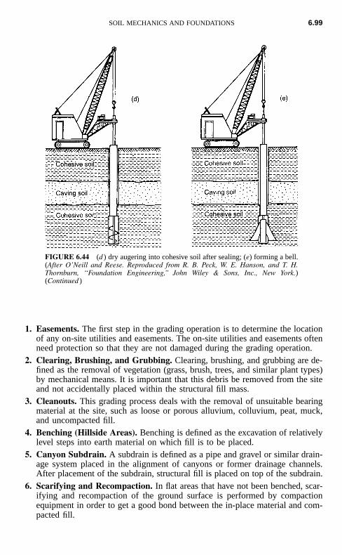
SOIL MECHANICS AND FOUNDATIONS 6.99
FIGURE 6.44 (d ) dry augering into cohesive soil after sealing; (e) forming a bell.(After O’Neill and Reese. Reproduced from R. B. Peck, W. E. Hanson, and T. H.Thornburn, ‘‘Foundation Engineering,’’ John Wiley & Sons, Inc., New York.)(Continued )
1. Easements. The first step in the grading operation is to determine the locationof any on-site utilities and easements. The on-site utilities and easements oftenneed protection so that they are not damaged during the grading operation.
2. Clearing, Brushing, and Grubbing. Clearing, brushing, and grubbing are de-fined as the removal of vegetation (grass, brush, trees, and similar plant types)by mechanical means. It is important that this debris be removed from the siteand not accidentally placed within the structural fill mass.
3. Cleanouts. This grading process deals with the removal of unsuitable bearingmaterial at the site, such as loose or porous alluvium, colluvium, peat, muck,and uncompacted fill.
4. Benching (Hillside Areas). Benching is defined as the excavation of relativelylevel steps into earth material on which fill is to be placed.
5. Canyon Subdrain. A subdrain is defined as a pipe and gravel or similar drain-age system placed in the alignment of canyons or former drainage channels.After placement of the subdrain, structural fill is placed on top of the subdrain.
6. Scarifying and Recompaction. In flat areas that have not been benched, scar-ifying and recompaction of the ground surface is performed by compactionequipment in order to get a good bond between the in-place material and com-pacted fill.
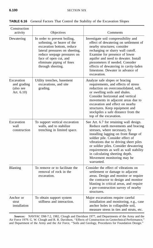
6.100 SECTION SIX
TABLE 6.16 General Factors That Control the Stability of the Excavation Slopes
Constructionactivity Objectives Comments
Dewatering In order to prevent boiling,softening, or heave of theexcavation bottom, reducelateral pressures on sheeting,reduce seepage pressures onface of open cut, andeliminate piping of finesthrough sheeting.
Investigate soil compressibility andeffect of dewatering on settlement ofnearby structures; considerrecharging or slurry wall cutoff.Examine for presence of loweraquifer and need to dewater. Installpiezometers if needed. Considereffects of dewatering in cavity-ladenlimestone. Dewater in advance ofexcavation.
Excavationand grading(also seeArt. 6.10)
Utility trenches, basementexcavations, and sitegrading.
Analyze safe slopes or bracingrequirements, and effects of stressreduction on overconsolidated, soft,or swelling soils and shales.Consider horizontal and verticalmovements in adjacent areas due toexcavation and effect on nearbystructures. Keep equipment andstockpiles a safe distance from thetop of the excavation.
Excavationwallconstruction
To support vertical excavationwalls, and to stabilizetrenching in limited space.
See Art. 6.7 for retaining wall design.Reduce earth movements and bracingstresses, where necessary, byinstalling lagging on front flange ofsoldier pile. Consider effect ofvibrations due to driving sheet pilesor soldier piles. Consider dewateringrequirements as well as wall stabilityin calculating sheeting depth.Movement monitoring may bewarranted.
Blasting To remove or to facilitate theremoval of rock in theexcavation.
Consider the effect of vibrations onsettlement or damage to adjacentareas. Design and monitor or requirethe contractor to design and monitorblasting in critical areas, and requirea pre-construction survey of nearbystructures.
Anchor orstrutinstallation
To obtain support systemstiffness and interaction.
Major excavations require carefulinstallation and monitoring, e.g., caseanchor holes in collapsible soil,measure stress in ties and struts, etc.
Sources: NAVFAC DM-7.2, 1982, Clough and Davidson 1977, and Departments of the Army and theAir Force 1979. G. W. Clough and R. R. Davidson, ‘‘Effects of Construction on Geotechnical Performance,’’and Department of the Army and the Air Force, ‘‘Soils and Geology, Procedures for Foundation Design.’’
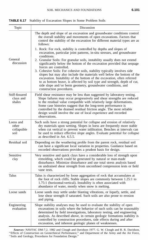
SOIL MECHANICS AND FOUNDATIONS 6.101
TABLE 6.17 Stability of Excavation Slopes in Some Problem Soils
Topic Discussion
Generaldiscussion
The depth and slope of an excavation and groundwater conditions controlthe overall stability and movements of open excavations. Factors thatcontrol the stability of the excavation for different material types are asfollows:
1. Rock: For rock, stability is controlled by depths and slopes ofexcavation, particular joint patterns, in-situ stresses, and groundwaterconditions.
2. Granular Soils: For granular soils, instability usually does not extendsignificantly below the bottom of the excavation provided that seepageforces are controlled.
3. Cohesive Soils: For cohesive soils, stability typically involves sideslopes but may also include the materials well below the bottom of theexcavation. Instability of the bottom of the excavation, often referredto as bottom heave, is affected by soil type and strength, depth of cut,side slope and /or berm geometry, groundwater conditions, andconstruction procedures.
Stiff-fissuredclays andshales
Field shear resistance may be less than suggested by laboratory testing.Slope failures may occur progressively and shear strengths are reducedto the residual value compatible with relatively large deformations.Some case histories suggest that the long-term performance iscontrolled by the drained residual friction angle. The most reliabledesign would involve the use of local experience and recordedobservations.
Loess andothercollapsiblesoil
Such soils have a strong potential for collapse and erosion of relativelydry materials upon wetting. Slopes in loess are frequently more stablewhen cut vertical to prevent water infiltration. Benches at intervals canbe used to reduce effective slope angles. Evaluate potential for collapseas described in Art. 6.5.5.
Residual soil Depending on the weathering profile from the parent rock, residual soilcan have a significant local variation in properties. Guidance based onrecorded observations provides a prudent basis for design.
Sensitiveclay
Very sensitive and quick clays have a considerable loss of strength uponremolding, which could be generated by natural or man-madedisturbance. Minimize disturbance and use total stress analysis basedon undrained shear strength from unconfined compression tests or fieldvane tests.
Talus Talus is characterized by loose aggregation of rock that accumulates atthe foot of rock cliffs. Stable slopes are commonly between 1.25:1 to1.75:1 (horizontal:vertical). Instability is often associated withabundance of water, mostly when snow is melting.
Loose sands Loose sands may settle under blasting vibrations, or liquefy, settle, andlose shear strength if saturated. Such soils are also prone to erosionand piping.
Engineeringevaluation
Slope stability analyses may be used to evaluate the stability of openexcavations in soils where the behavior of such soils can be reasonablydetermined by field investigations, laboratory testing, and engineeringanalysis. As described above, in certain geologic formations stability iscontrolled by construction procedures, side effects during and afterexcavation, and inherent geologic planes of weaknesses.
Sources: NAVFAC DM-7.2, 1982 and Clough and Davidson 1977. G. W. Clough and R. R. Davidson,‘‘Effects of Construction on Geotechnical Performance,’’ and Department of the Army and the Air Force,‘‘Soils and Geology, Procedures for Foundation Design.’’
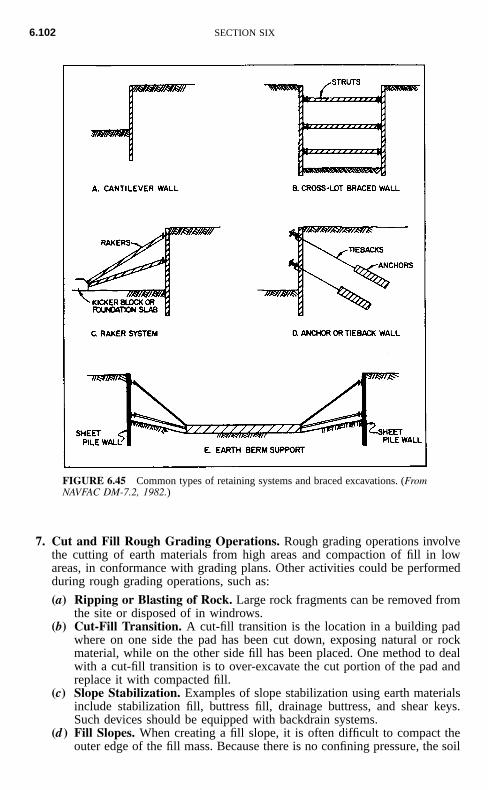
6.102 SECTION SIX
FIGURE 6.45 Common types of retaining systems and braced excavations. (FromNAVFAC DM-7.2, 1982.)
7. Cut and Fill Rough Grading Operations. Rough grading operations involvethe cutting of earth materials from high areas and compaction of fill in lowareas, in conformance with grading plans. Other activities could be performedduring rough grading operations, such as:
(a) Ripping or Blasting of Rock. Large rock fragments can be removed fromthe site or disposed of in windrows.
(b) Cut-Fill Transition. A cut-fill transition is the location in a building padwhere on one side the pad has been cut down, exposing natural or rockmaterial, while on the other side fill has been placed. One method to dealwith a cut-fill transition is to over-excavate the cut portion of the pad andreplace it with compacted fill.
(c) Slope Stabilization. Examples of slope stabilization using earth materialsinclude stabilization fill, buttress fill, drainage buttress, and shear keys.Such devices should be equipped with backdrain systems.
(d ) Fill Slopes. When creating a fill slope, it is often difficult to compact theouter edge of the fill mass. Because there is no confining pressure, the soil
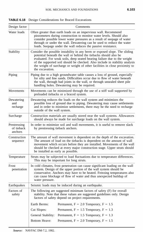
SOIL MECHANICS AND FOUNDATIONS 6.103
TABLE 6.18 Design Considerations for Braced Excavations
Design factor Comments
Water loads Often greater than earth loads on an impervious wall. Recommendpiezometers during construction to monitor water levels. Should alsoconsider possible lower water pressures as a result of seepage of waterthrough or under the wall. Dewatering can be used to reduce the waterloads. Seepage under the wall reduces the passive resistance.
Stability Consider the possible instability in any berm or exposed slope. The slidingpotential beneath the wall or behind the tiebacks should also beevaluated. For weak soils, deep seated bearing failure due to the weightof the supported soil should be checked. Also include in stability analysisthe weight of surcharge or weight of other facilities in close proximity tothe excavation.
Piping Piping due to a high groundwater table causes a loss of ground, especiallyfor silty and fine sands. Difficulties occur due to flow of water beneaththe wall, through bad joints in the wall, or through unsealed sheet pilehandling holes. Dewatering may be required.
Movements Movements can be minimized through the use of a stiff wall supported bypreloaded tiebacks or a braced system.
Dewateringandrecharge
Dewatering reduces the loads on the wall system and minimizes thepossible loss of ground due to piping. Dewatering may cause settlementsand in order to minimize settlements, there may be the need to rechargeoutside of the wall system.
Surcharge Construction materials are usually stored near the wall systems. Allowancesshould always be made for surcharge loads on the wall system.
Prestressingof tiebackanchors
In order to minimize soil and wall movements, it is useful to remove slackby prestressing tieback anchors.
Constructionsequence
The amount of wall movement is dependent on the depth of the excavation.The amount of load on the tiebacks is dependent on the amount of wallmovement which occurs before they are installed. Movements of the wallshould be checked at every major construction stage. Upper struts shouldbe installed as early as possible.
Temperature Struts may be subjected to load fluctuations due to temperature differences.This may be important for long struts.
Frostpenetration
In cold climates, frost penetration can cause significant loading on the wallsystem. Design of the upper portion of the wall system should beconservative. Anchors may have to be heated. Freezing temperatures alsocan cause blockage of flow of water and thus unexpected buildup ofwater pressure.
Earthquakes Seismic loads may be induced during an earthquake.
Factors ofsafety
The following are suggested minimum factors of safety (F) for overallstability. Note that these values are suggested guidelines only. Designfactors of safety depend on project requirements.
Earth Berms: Permanent, F � 2.0 Temporary, F � 1.5
Cut Slopes: Permanent, F � 1.5 Temporary, F � 1.3
General Stability: Permanent, F � 1.5 Temporary, F � 1.3
Bottom Heave: Permanent, F � 2.0 Temporary, F � 1.5
Source: NAVFAC DM-7.2, 1982.
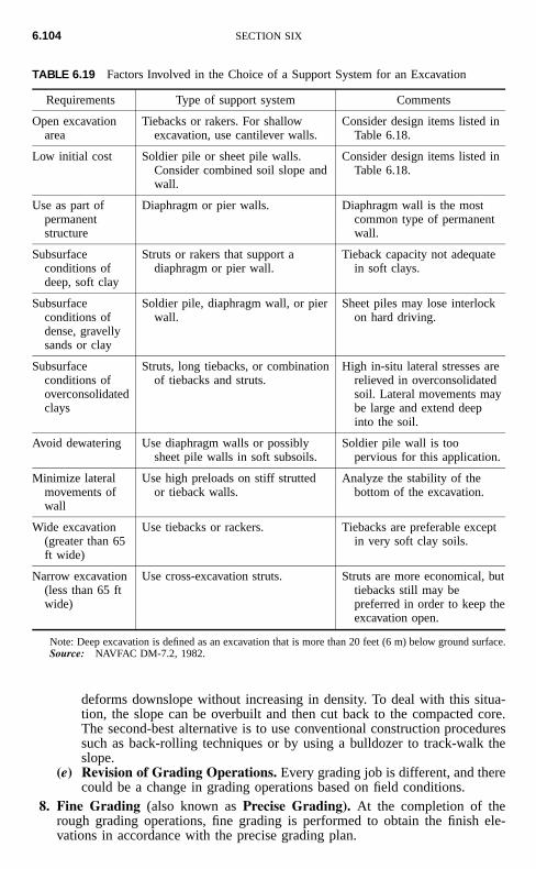
6.104 SECTION SIX
TABLE 6.19 Factors Involved in the Choice of a Support System for an Excavation
Requirements Type of support system Comments
Open excavationarea
Tiebacks or rakers. For shallowexcavation, use cantilever walls.
Consider design items listed inTable 6.18.
Low initial cost Soldier pile or sheet pile walls.Consider combined soil slope andwall.
Consider design items listed inTable 6.18.
Use as part ofpermanentstructure
Diaphragm or pier walls. Diaphragm wall is the mostcommon type of permanentwall.
Subsurfaceconditions ofdeep, soft clay
Struts or rakers that support adiaphragm or pier wall.
Tieback capacity not adequatein soft clays.
Subsurfaceconditions ofdense, gravellysands or clay
Soldier pile, diaphragm wall, or pierwall.
Sheet piles may lose interlockon hard driving.
Subsurfaceconditions ofoverconsolidatedclays
Struts, long tiebacks, or combinationof tiebacks and struts.
High in-situ lateral stresses arerelieved in overconsolidatedsoil. Lateral movements maybe large and extend deepinto the soil.
Avoid dewatering Use diaphragm walls or possiblysheet pile walls in soft subsoils.
Soldier pile wall is toopervious for this application.
Minimize lateralmovements ofwall
Use high preloads on stiff struttedor tieback walls.
Analyze the stability of thebottom of the excavation.
Wide excavation(greater than 65ft wide)
Use tiebacks or rackers. Tiebacks are preferable exceptin very soft clay soils.
Narrow excavation(less than 65 ftwide)
Use cross-excavation struts. Struts are more economical, buttiebacks still may bepreferred in order to keep theexcavation open.
Note: Deep excavation is defined as an excavation that is more than 20 feet (6 m) below ground surface.Source: NAVFAC DM-7.2, 1982.
deforms downslope without increasing in density. To deal with this situa-tion, the slope can be overbuilt and then cut back to the compacted core.The second-best alternative is to use conventional construction proceduressuch as back-rolling techniques or by using a bulldozer to track-walk theslope.
(e) Revision of Grading Operations. Every grading job is different, and therecould be a change in grading operations based on field conditions.
8. Fine Grading (also known as Precise Grading). At the completion of therough grading operations, fine grading is performed to obtain the finish ele-vations in accordance with the precise grading plan.
SOIL MECHANICS AND FOUNDATIONS 6.105
9. Slope Protection and Erosion Control. Although this is usually not the re-sponsibility of the grading contractor, upon completion of the fine grading,slope protection and permanent erosion control devices are installed.
10. Trench Excavations. Utility trenches are excavated in the proposed road align-ments and building pads for the installation of the on-site utilities. The exca-vation and compaction of utility trenches is often part of the grading process.Once the utility lines are installed, scarifying and recompaction of the roadsubgrade is performed and base material is placed and compacted.
11. Footing and Foundation Excavations. Although this is usually not part of thegrading operation, the footing and foundation elements are then excavated (seeArt. 6.9).
6.10.1 Compaction Fundamentals
An important part of the grading of the site often includes the compaction of fill.Compaction is defined as the densification of a fill by mechanical means. Thisphysical process of getting the soil into a dense state can increase the shear strength,decrease the compressibility, and decrease the permeability of the soil. There arefour basic factors that affect compaction:
1. Soil Type. Nonplastic (i.e., granular) soil, such as sands and gravels, can beeffectively compacted by using a vibrating or shaking type of compaction op-eration. Plastic (i.e., cohesive) soil, such as silts and clays, is more difficult tocompact and requires a kneading or manipulation type of compaction operation.If the soil contains oversize particles, such as coarse gravel and cobbles, theseparticles tend to interfere with the compaction process and reduce the effective-ness of compaction for the finer soil particles. Typical values of dry density fordifferent types of compacted soil are listed in Table 6.20.
2. Material Gradation. Those soils that have a well-graded grain size distributioncan generally be compacted into a denser state than a poorly graded soil that iscomposed of soil particles of about the same size. For example, a well-gradeddecomposed granite (DG) can have a maximum dry density of 2.2 Mg/m3 (137pcf), while a poorly graded sand can have a maximum dry density of only 1.6Mg/m3 (100 pcf, Modified Proctor).
3. Water Content. The water content is an important parameter in the compactionof soil. Water tends to lubricate the soil particles thus helping them slide intodense arrangements. However, too much water and the soil becomes saturatedand often difficult to compact. There is an optimum water content at which thesoil can be compacted into its densest state for a given compaction energy.Typical optimum moisture contents (Modified Proctor) for different soil typesare as follows:
(a) Clay of High Plasticity (CH): optimum moisture content � 18%(b) Clay of Low Plasticity (CL): optimum moisture content � 12 to 18%(c) Well-Graded Sand (SW): optimum moisture content � 10%(d ) Well-Graded Gravel (GW): optimum moisture content � 7%
Some soils may be relatively insensitive to compaction water content. Forexample, open-graded gravels and clean coarse sands are so permeable that watersimply drains out of the soil or is forced out of the soil during the compactionprocess. These types of soil can often be placed in a dry state and then vibratedinto dense particle arrangements.
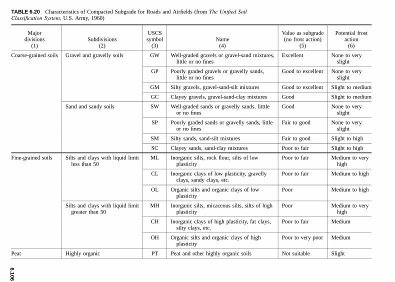
6.1
06
TABLE 6.20 Characteristics of Compacted Subgrade for Roads and Airfields (from The Unified SoilClassification System, U.S. Army, 1960)
Majordivisions
(1)Subdivisions
(2)
USCSsymbol
(3)Name
(4)
Value as subgrade(no frost action)
(5)
Potential frostaction
(6)
Coarse-grained soils Gravel and gravelly soils GW Well-graded gravels or gravel-sand mixtures,little or no fines
Excellent None to veryslight
GP Poorly graded gravels or gravelly sands,little or no fines
Good to excellent None to veryslight
GM Silty gravels, gravel-sand-silt mixtures Good to excellent Slight to medium
GC Clayey gravels, gravel-sand-clay mixtures Good Slight to medium
Sand and sandy soils SW Well-graded sands or gravelly sands, litttleor no fines
Good None to veryslight
SP Poorly graded sands or gravelly sands, littleor no fines
Fair to good None to veryslight
SM Silty sands, sand-silt mixtures Fair to good Slight to high
SC Clayey sands, sand-clay mixtures Poor to fair Slight to high
Fine-grained soils Silts and clays with liquid limitless than 50
ML Inorganic silts, rock flour, silts of lowplasticity
Poor to fair Medium to veryhigh
CL Inorganic clays of low plasticity, gravellyclays, sandy clays, etc.
Poor to fair Medium to high
OL Organic silts and organic clays of lowplasticity
Poor Medium to high
Silts and clays with liquid limitgreater than 50
MH Inorganic silts, micaceous silts, silts of highplasticity
Poor Medium to veryhigh
CH Inorganic clays of high plasticity, fat clays,silty clays, etc.
Poor to fair Medium
OH Organic silts and organic clays of highplasticity
Poor to very poor Medium
Peat Highly organic PT Peat and other highly organic soils Not suitable Slight
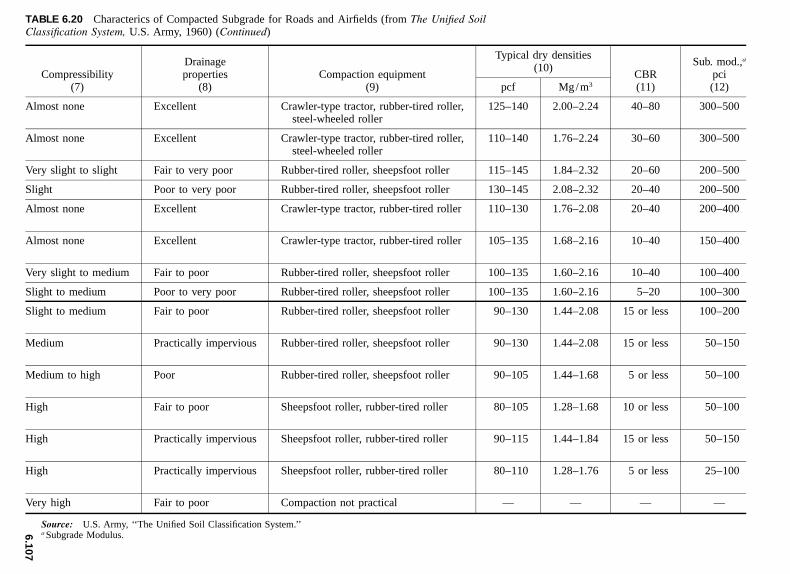
6.1
07
TABLE 6.20 Characterics of Compacted Subgrade for Roads and Airfields (from The Unified SoilClassification System, U.S. Army, 1960) (Continued)
Compressibility(7)
Drainageproperties
(8)Compaction equipment
(9)
Typical dry densities(10)
pcf Mg/m3CBR(11)
Sub. mod.,a
pci(12)
Almost none Excellent Crawler-type tractor, rubber-tired roller,steel-wheeled roller
125–140 2.00–2.24 40–80 300–500
Almost none Excellent Crawler-type tractor, rubber-tired roller,steel-wheeled roller
110–140 1.76–2.24 30–60 300–500
Very slight to slight Fair to very poor Rubber-tired roller, sheepsfoot roller 115–145 1.84–2.32 20–60 200–500
Slight Poor to very poor Rubber-tired roller, sheepsfoot roller 130–145 2.08–2.32 20–40 200–500
Almost none Excellent Crawler-type tractor, rubber-tired roller 110–130 1.76–2.08 20–40 200–400
Almost none Excellent Crawler-type tractor, rubber-tired roller 105–135 1.68–2.16 10–40 150–400
Very slight to medium Fair to poor Rubber-tired roller, sheepsfoot roller 100–135 1.60–2.16 10–40 100–400
Slight to medium Poor to very poor Rubber-tired roller, sheepsfoot roller 100–135 1.60–2.16 5–20 100–300
Slight to medium Fair to poor Rubber-tired roller, sheepsfoot roller 90–130 1.44–2.08 15 or less 100–200
Medium Practically impervious Rubber-tired roller, sheepsfoot roller 90–130 1.44–2.08 15 or less 50–150
Medium to high Poor Rubber-tired roller, sheepsfoot roller 90–105 1.44–1.68 5 or less 50–100
High Fair to poor Sheepsfoot roller, rubber-tired roller 80–105 1.28–1.68 10 or less 50–100
High Practically impervious Sheepsfoot roller, rubber-tired roller 90–115 1.44–1.84 15 or less 50–150
High Practically impervious Sheepsfoot roller, rubber-tired roller 80–110 1.28–1.76 5 or less 25–100
Very high Fair to poor Compaction not practical — — — —
Source: U.S. Army, ‘‘The Unified Soil Classification System.’’a Subgrade Modulus.
6.108 SECTION SIX
4. Compaction Effort (or Energy). The compactive effort is a measure of themechanical energy applied to the soil. Usually, the greater the amount of com-paction energy applied to a soil, the denser the soil will become. There areexceptions, such as pumping soils (i.e., saturated clays), which can not be den-sified by an increased compaction effort. Compactors are designed to use oneor a combination of the following types of compaction effort:
(a) Static weight or pressure(b) Kneading action or manipulation(c) Impact or a sharp blow(d ) Vibration or shaking
The laboratory compaction test consists of compacting a soil at a known watercontent into a mold of specific dimensions using a certain compaction energy. Theprocedure is repeated for various water contents to establish the compaction curve.The most common testing procedures (compaction energy, number of soil layers inthe mold, etc.) are the Modified Proctor (ASTM D 1557-91, 1998) and the StandardProctor (ASTM D 698-91, 1998). The term Proctor is in honor of R. R. Proctor,who in 1933 showed that the dry density of a soil for a given compactive effortdepends on the amount of water the soil contains during compaction.
For the Modified Proctor (ASTM D 1557-91, 1998, procedure A), the soil iscompacted into a 10.2-cm (4-in) diameter mold that has a volume of 944 cm3
(1/30 ft3), where five layers of soil are compacted into the mold, with each layerreceiving 25 blows from a 44.5-N (10-lbf) hammer that has a 0.46-m (18-in) drop.The Modified Proctor has a compaction energy of 2700 kN-m/m3 (56,000 ft-lbf /ft3). The test procedure is to prepare soil at a certain water content, compact thesoil into the mold, and then, by recording the mass of soil within the mold, obtainthe wet density of the compacted soil. By measuring the water content of thecompacted soil, the dry density can be calculated. This compaction procedure isrepeated for the soil at different water contents and then the data are plotted on agraph in order to obtain the compaction curve.
Figure 6.46 shows the compaction curves for various soils using the ModifiedProctor compaction test. The compaction curves show the relationship between thedry density (or dry unit weight) and water content for a given compaction effort.The compaction data presented in Fig. 6.46 were obtained using the Modified Proc-tor specifications. The lines to the right of the compaction curves are each knownas a zero air voids curve. These curves represent a condition of saturation (S �100%) for a specified specific gravity. Note how the right side of the compactioncurves are approximately parallel to the zero air voids curve. This is often the casefor many soil types and can be used as a check on the laboratory test results.
The peak point of the compaction curve is the laboratory maximum dry density(or the maximum dry unit weight). The water content corresponding to the labo-ratory maximum dry density is known as the optimum moisture content. Theselaboratory data are important because it tells the grading contractor the best watercontent for the most efficient compaction of the soil.
The most common method of assessing the quality of the field compaction is tocalculate the relative compaction (RC) of the fill, defined as: RC � 100 �d /�d max,where �d max � laboratory maximum dry density and �d � field dry density. Themaximum dry density (�d max) is the peak point of the laboratory compaction curve.In order for �d to be determined, a field density test must be performed. Fielddensity tests can be classified as either destructive or nondestructive tests. Probablythe most common destructive method of determining the field dry density is through
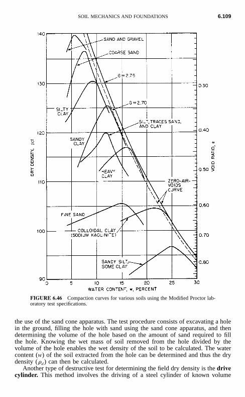
SOIL MECHANICS AND FOUNDATIONS 6.109
FIGURE 6.46 Compaction curves for various soils using the Modified Proctor lab-oratory test specifications.
the use of the sand cone apparatus. The test procedure consists of excavating a holein the ground, filling the hole with sand using the sand cone apparatus, and thendetermining the volume of the hole based on the amount of sand required to fillthe hole. Knowing the wet mass of soil removed from the hole divided by thevolume of the hole enables the wet density of the soil to be calculated. The watercontent (w) of the soil extracted from the hole can be determined and thus the drydensity (�d ) can then be calculated.
Another type of destructive test for determining the field dry density is the drivecylinder. This method involves the driving of a steel cylinder of known volume
6.110 SECTION SIX
into the soil. Based on the mass of soil within the cylinder, the wet density can becalculated. Once the water content (w) of the soil is obtained, the dry density(�d ) of the fill can be calculated.
Probably the most common type of nondestructive field test is the nuclearmethod. In this method, the wet density is determined by the attenuation of gammaradiation. The nuclear method can give inaccurate results (density too high) whereoversize particles are present, such as coarse gravel and cobbles. Likewise, if thereis a large void in the source-detector path, then unusually low density values maybe recorded.
6.10.2 Site Improvement Methods
If the expected settlement for a proposed structure is too large, then different foun-dation support or soil stabilization options must be evaluated. As discussed in Art.6.8.2, one alternative is a deep foundation system that can transfer structural loadsto adequate bearing material in order to bypass a compressible soil layer. Anotheroption is to construct a floating foundation, which is a special type of deep foun-dation where the weight of the structure is balanced by the removal of soil andconstruction of an underground basement. Other alternatives include site improve-ment methods, such as the following (see Table 6.21):
Soil Replacement. As indicated in Table 6.21, there are basically two types ofsoil replacement methods: (1) removal and replacement, and (2) displacement.The first is the most common approach and consists of the removal of the com-pressible soil layer and replacement with structural fill during the grading op-erations. Usually the remove and replace grading option is economical only ifthe compressible soil layer is near the ground surface and the groundwater tableis below the compressible soil layer or the groundwater table can be economi-cally lowered.Water Removal. Table 6.21 lists several different types of water removal siteimprovement techniques. If the site contains an underlying compressible cohe-sive soil layer, the site can be surcharged with a fill layer placed at groundsurface. Vertical drains (such as wick drains or sand drains) can be installed inthe compressible soil layer to reduce the drainage path and speed up the con-solidation process. Once the compressible cohesive soil layer has had sufficientconsolidation, the fill surcharge layer is removed and the building is constructed.Site Strengthening. Many different methods can be used to strengthen the on-site soil (see Table 6.21). For example, deep vibratory techniques are often usedto increase the density of loose sand deposits.Grouting. In order to stabilize the ground, fluid grout can be injected into theground to fill in joints, fractures, or underground voids. For the releveling ofexisting structures, one option is mudjacking, which has been defined as a pro-cess whereby a water and soil-cement or soil-lime cement grout is pumpedbeneath the slab, under pressure, to produce a lifting force that literally floatsthe slab to the desired position. Another commonly used site improvement tech-nique is compaction grouting, which consists of intruding a mass of very thick-consistency grout into the soil, which both displaces and compacts the loosesoil. Compaction grouting has proved successful in increasing the density ofpoorly compacted fill, alluvium, and compressible or collapsible soil. The ad-vantages of compaction grouting are less expense and disturbance to the structure
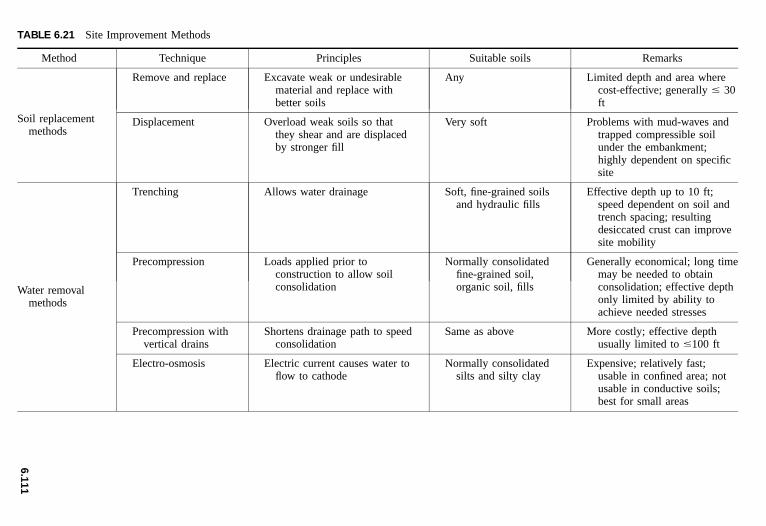
6.1
11
TABLE 6.21 Site Improvement Methods
Method Technique Principles Suitable soils Remarks
Soil replacementmethods
Remove and replace
Displacement
Excavate weak or undesirablematerial and replace withbetter soils
Overload weak soils so thatthey shear and are displacedby stronger fill
Any
Very soft
Limited depth and area wherecost-effective; generally � 30ft
Problems with mud-waves andtrapped compressible soilunder the embankment;highly dependent on specificsite
Water removalmethods
Trenching
Precompression
Precompression withvertical drains
Electro-osmosis
Allows water drainage
Loads applied prior toconstruction to allow soilconsolidation
Shortens drainage path to speedconsolidation
Electric current causes water toflow to cathode
Soft, fine-grained soilsand hydraulic fills
Normally consolidatedfine-grained soil,organic soil, fills
Same as above
Normally consolidatedsilts and silty clay
Effective depth up to 10 ft;speed dependent on soil andtrench spacing; resultingdesiccated crust can improvesite mobility
Generally economical; long timemay be needed to obtainconsolidation; effective depthonly limited by ability toachieve needed stresses
More costly; effective depthusually limited to �100 ft
Expensive; relatively fast;usable in confined area; notusable in conductive soils;best for small areas
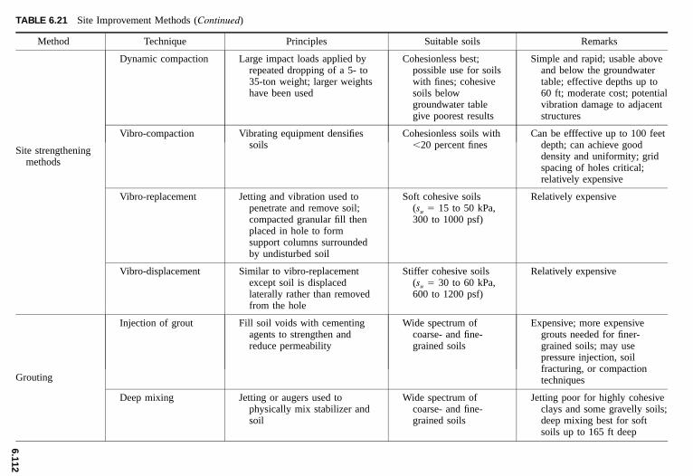
6.1
12
TABLE 6.21 Site Improvement Methods (Continued)
Method Technique Principles Suitable soils Remarks
Site strengtheningmethods
Dynamic compaction
Vibro-compaction
Vibro-replacement
Large impact loads applied byrepeated dropping of a 5- to35-ton weight; larger weightshave been used
Vibrating equipment densifiessoils
Jetting and vibration used topenetrate and remove soil;compacted granular fill thenplaced in hole to formsupport columns surroundedby undisturbed soil
Cohesionless best;possible use for soilswith fines; cohesivesoils belowgroundwater tablegive poorest results
Cohesionless soils with�20 percent fines
Soft cohesive soils(su � 15 to 50 kPa,300 to 1000 psf)
Simple and rapid; usable aboveand below the groundwatertable; effective depths up to60 ft; moderate cost; potentialvibration damage to adjacentstructures
Can be efffective up to 100 feetdepth; can achieve gooddensity and uniformity; gridspacing of holes critical;relatively expensive
Relatively expensive
Vibro-displacement Similar to vibro-replacementexcept soil is displacedlaterally rather than removedfrom the hole
Stiffer cohesive soils(su � 30 to 60 kPa,600 to 1200 psf)
Relatively expensive
Grouting
Injection of grout
Deep mixing
Fill soil voids with cementingagents to strengthen andreduce permeability
Jetting or augers used tophysically mix stabilizer andsoil
Wide spectrum ofcoarse- and fine-grained soils
Wide spectrum ofcoarse- and fine-grained soils
Expensive; more expensivegrouts needed for finer-grained soils; may usepressure injection, soilfracturing, or compactiontechniques
Jetting poor for highly cohesiveclays and some gravelly soils;deep mixing best for softsoils up to 165 ft deep
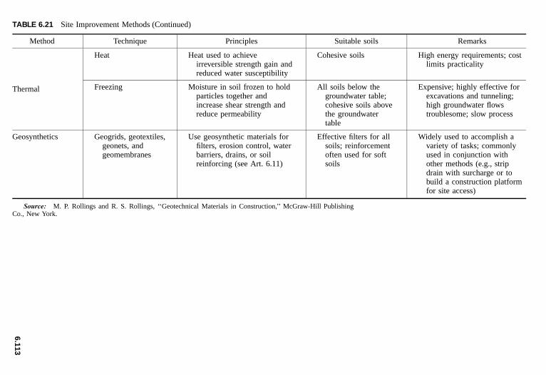
6.1
13
Thermal
Heat
Freezing
Heat used to achieveirreversible strength gain andreduced water susceptibility
Moisture in soil frozen to holdparticles together andincrease shear strength andreduce permeability
Cohesive soils
All soils below thegroundwater table;cohesive soils abovethe groundwatertable
High energy requirements; costlimits practicality
Expensive; highly effective forexcavations and tunneling;high groundwater flowstroublesome; slow process
Geosynthetics Geogrids, geotextiles,geonets, andgeomembranes
Use geosynthetic materials forfilters, erosion control, waterbarriers, drains, or soilreinforcing (see Art. 6.11)
Effective filters for allsoils; reinforcementoften used for softsoils
Widely used to accomplish avariety of tasks; commonlyused in conjunction withother methods (e.g., stripdrain with surcharge or tobuild a construction platformfor site access)
Source: M. P. Rollings and R. S. Rollings, ‘‘Geotechnical Materials in Construction,’’ McGraw-Hill PublishingCo., New York.
TABLE 6.21 Site Improvement Methods (Continued)
Method Technique Principles Suitable soils Remarks
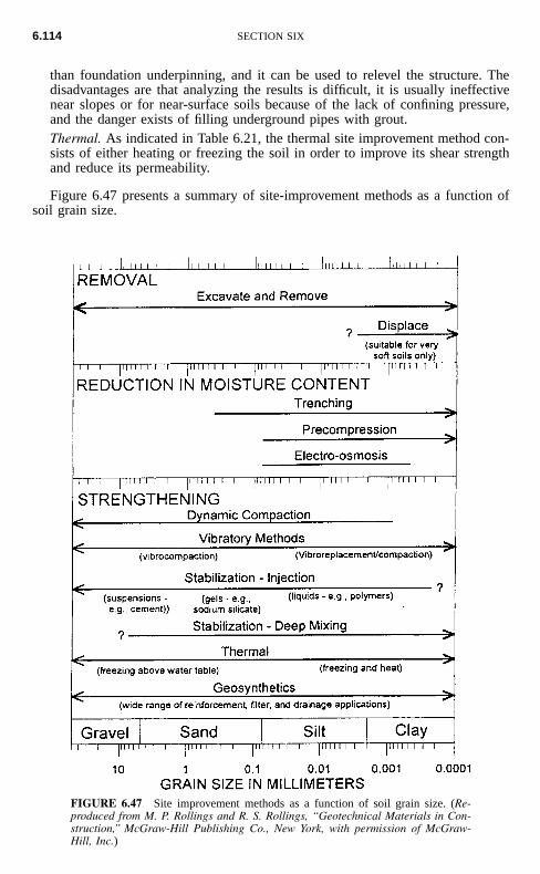
6.114 SECTION SIX
FIGURE 6.47 Site improvement methods as a function of soil grain size. (Re-produced from M. P. Rollings and R. S. Rollings, ‘‘Geotechnical Materials in Con-struction,’’ McGraw-Hill Publishing Co., New York, with permission of McGraw-Hill, Inc.)
than foundation underpinning, and it can be used to relevel the structure. Thedisadvantages are that analyzing the results is difficult, it is usually ineffectivenear slopes or for near-surface soils because of the lack of confining pressure,and the danger exists of filling underground pipes with grout.Thermal. As indicated in Table 6.21, the thermal site improvement method con-sists of either heating or freezing the soil in order to improve its shear strengthand reduce its permeability.
Figure 6.47 presents a summary of site-improvement methods as a function ofsoil grain size.
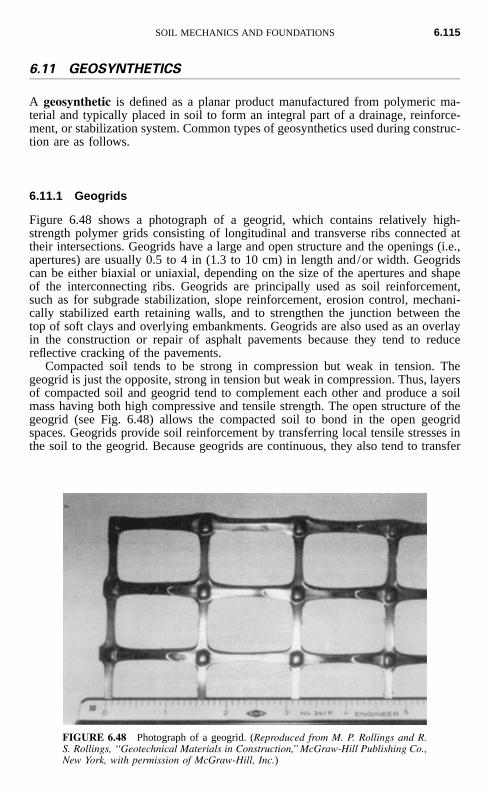
SOIL MECHANICS AND FOUNDATIONS 6.115
FIGURE 6.48 Photograph of a geogrid. (Reproduced from M. P. Rollings and R.S. Rollings, ‘‘Geotechnical Materials in Construction,’’ McGraw-Hill Publishing Co.,New York, with permission of McGraw-Hill, Inc.)
6.11 GEOSYNTHETICS
A geosynthetic is defined as a planar product manufactured from polymeric ma-terial and typically placed in soil to form an integral part of a drainage, reinforce-ment, or stabilization system. Common types of geosynthetics used during construc-tion are as follows.
6.11.1 Geogrids
Figure 6.48 shows a photograph of a geogrid, which contains relatively high-strength polymer grids consisting of longitudinal and transverse ribs connected attheir intersections. Geogrids have a large and open structure and the openings (i.e.,apertures) are usually 0.5 to 4 in (1.3 to 10 cm) in length and/or width. Geogridscan be either biaxial or uniaxial, depending on the size of the apertures and shapeof the interconnecting ribs. Geogrids are principally used as soil reinforcement,such as for subgrade stabilization, slope reinforcement, erosion control, mechani-cally stabilized earth retaining walls, and to strengthen the junction between thetop of soft clays and overlying embankments. Geogrids are also used as an overlayin the construction or repair of asphalt pavements because they tend to reducereflective cracking of the pavements.
Compacted soil tends to be strong in compression but weak in tension. Thegeogrid is just the opposite, strong in tension but weak in compression. Thus, layersof compacted soil and geogrid tend to complement each other and produce a soilmass having both high compressive and tensile strength. The open structure of thegeogrid (see Fig. 6.48) allows the compacted soil to bond in the open geogridspaces. Geogrids provide soil reinforcement by transferring local tensile stresses inthe soil to the geogrid. Because geogrids are continuous, they also tend to transfer
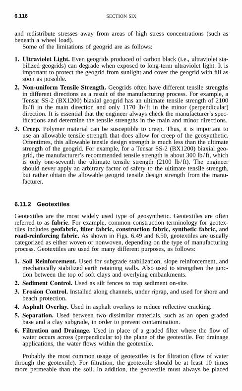
6.116 SECTION SIX
and redistribute stresses away from areas of high stress concentrations (such asbeneath a wheel load).
Some of the limitations of geogrid are as follows:
1. Ultraviolet Light. Even geogrids produced of carbon black (i.e., ultraviolet sta-bilized geogrids) can degrade when exposed to long-term ultraviolet light. It isimportant to protect the geogrid from sunlight and cover the geogrid with fill assoon as possible.
2. Non-uniform Tensile Strength. Geogrids often have different tensile strengthsin different directions as a result of the manufacturing process. For example, aTensar SS-2 (BX1200) biaxial geogrid has an ultimate tensile strength of 2100lb/ ft in the main direction and only 1170 lb/ ft in the minor (perpendicular)direction. It is essential that the engineer always check the manufacturer’s spec-ifications and determine the tensile strengths in the main and minor directions.
3. Creep. Polymer material can be susceptible to creep. Thus, it is important touse an allowable tensile strength that does allow for creep of the geosynthetic.Oftentimes, this allowable tensile design strength is much less than the ultimatestrength of the geogrid. For example, for a Tensar SS-2 (BX1200) biaxial geo-grid, the manufacturer’s recommended tensile strength is about 300 lb/ ft, whichis only one-seventh the ultimate tensile strength (2100 lb/ ft). The engineershould never apply an arbitrary factor of safety to the ultimate tensile strength,but rather obtain the allowable geogrid tensile design strength from the manu-facturer.
6.11.2 Geotextiles
Geotextiles are the most widely used type of geosynthetic. Geotextiles are oftenreferred to as fabric. For example, common construction terminology for geotex-tiles includes geofabric, filter fabric, construction fabric, synthetic fabric, androad-reinforcing fabric. As shown in Figs. 6.49 and 6.50, geotextiles are usuallycategorized as either woven or nonwoven, depending on the type of manufacturingprocess. Geotextiles are used for many different purposes, as follows:
1. Soil Reinforcement. Used for subgrade stabilization, slope reinforcement, andmechanically stabilized earth retaining walls. Also used to strengthen the junc-tion between the top of soft clays and overlying embankments.
2. Sediment Control. Used as silt fences to trap sediment on-site.3. Erosion Control. Installed along channels, under riprap, and used for shore and
beach protection.4. Asphalt Overlay. Used in asphalt overlays to reduce reflective cracking.5. Separation. Used between two dissimilar materials, such as an open graded
base and a clay subgrade, in order to prevent contamination.6. Filtration and Drainage. Used in place of a graded filter where the flow of
water occurs across (perpendicular to) the plane of the geotextile. For drainageapplications, the water flows within the geotextile.
Probably the most common usage of geotextiles is for filtration (flow of waterthrough the geotextile). For filtration, the geotextile should be at least 10 timesmore permeable than the soil. In addition, the geotextile must always be placed
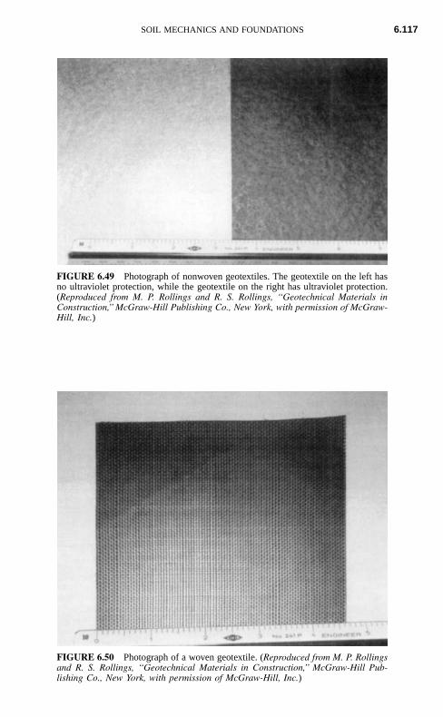
SOIL MECHANICS AND FOUNDATIONS 6.117
FIGURE 6.49 Photograph of nonwoven geotextiles. The geotextile on the left hasno ultraviolet protection, while the geotextile on the right has ultraviolet protection.(Reproduced from M. P. Rollings and R. S. Rollings, ‘‘Geotechnical Materials inConstruction,’’ McGraw-Hill Publishing Co., New York, with permission of McGraw-Hill, Inc.)
FIGURE 6.50 Photograph of a woven geotextile. (Reproduced from M. P. Rollingsand R. S. Rollings, ‘‘Geotechnical Materials in Construction,’’ McGraw-Hill Pub-lishing Co., New York, with permission of McGraw-Hill, Inc.)
6.118 SECTION SIX
between a less permeable (i.e., the soil) and a more permeable (i.e., the open gradedgravel) material. An inappropriate use of a geotextile would be to wrap it arounda drainage pipe and then cover the geotextile with open-graded gravel. This isbecause the geotextile would then have more permeable material on both sides ofthe geotextile and it would tend to restrict flow.
Two important design properties for geotextiles used as filtration devices are thatthey have an adequate flow capacity and a proper soil retention capability:
1. Flow Capacity. Although specifications have been developed that limit the openarea of the filtration geotextile to 10% or even 5%, it is best to have a largeropen area to develop an adequate flow capacity.
2. Soil Retention Capability. The apparent opening size (AOS), also known asthe equivalent opening size (EOS), determines the soil retention capability. TheAOS is often expressed in terms of opening size (mm) or equivalent sieve size(e.g., AOS � 40–70 indicates openings equivalent to the No. 40 to No. 70sieves). Obviously, if the geotextile openings are larger than the largest soilparticle diameter, then all of the soil particles will migrate through the geotextileand clog the drainage system. A common recommendation is that the requiredAOS be less than or equal to D85 (grain size corresponding to 85% percentpassing).
Some of the limitations of geotextile are as follows:
1. Ultraviolet Light. Geotextile that has no ultraviolet light protection can rapidlydeteriorate. For example, certain polypropylene geotextiles lost 100% of theirstrength after only 8 weeks of exposure.
2. Sealing of Geotextile. When the geotextile is used for filtration, an impermeablesoil layer can develop adjacent the geotextile if it has too low an open area ortoo small an AOS.
3. Construction Problems. Some of the more common problems related to con-struction with geotextiles are as follows (G. N. Richardson and D. C. Wyant,‘‘Geotextiles Construction Criteria’’):
(a) Fill placement or compaction techniques damage the geotextile.(b) Installation loads are greater than design loads, leading to failure during
construction.(c) Construction environment leads to a significant reduction in assumed fabric
properties, causing failure of the completed project.(d ) Field seaming or overlap of the geotextile fails to fully develop desired
fabric mechanical properties.(e) Instabilities during various construction phases may render a design inade-
quate even though the final product would have been stable.
6.11.3 Geomembranes
Common construction terminology for geomembranes includes liners, membranes,visqueen, plastic sheets, and impermeable sheets. Geomembranes are used almostexclusively as barriers to reduce water or vapor migration through soil (see Fig.6.51). For example, a common usage for geomembranes is for the lining and cap-ping systems in municipal landfills. For liners in municipal landfills, the thickness
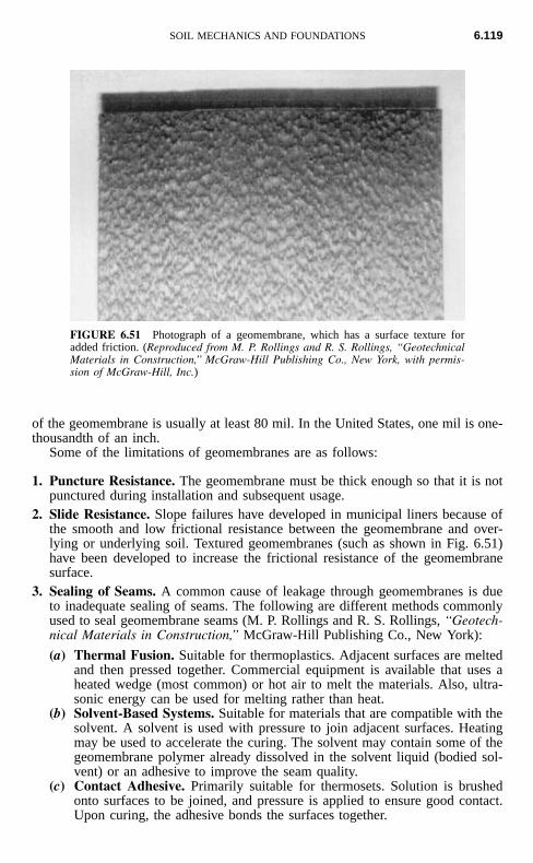
SOIL MECHANICS AND FOUNDATIONS 6.119
FIGURE 6.51 Photograph of a geomembrane, which has a surface texture foradded friction. (Reproduced from M. P. Rollings and R. S. Rollings, ‘‘GeotechnicalMaterials in Construction,’’ McGraw-Hill Publishing Co., New York, with permis-sion of McGraw-Hill, Inc.)
of the geomembrane is usually at least 80 mil. In the United States, one mil is one-thousandth of an inch.
Some of the limitations of geomembranes are as follows:
1. Puncture Resistance. The geomembrane must be thick enough so that it is notpunctured during installation and subsequent usage.
2. Slide Resistance. Slope failures have developed in municipal liners because ofthe smooth and low frictional resistance between the geomembrane and over-lying or underlying soil. Textured geomembranes (such as shown in Fig. 6.51)have been developed to increase the frictional resistance of the geomembranesurface.
3. Sealing of Seams. A common cause of leakage through geomembranes is dueto inadequate sealing of seams. The following are different methods commonlyused to seal geomembrane seams (M. P. Rollings and R. S. Rollings, ‘‘Geotech-nical Materials in Construction,’’ McGraw-Hill Publishing Co., New York):
(a) Thermal Fusion. Suitable for thermoplastics. Adjacent surfaces are meltedand then pressed together. Commercial equipment is available that uses aheated wedge (most common) or hot air to melt the materials. Also, ultra-sonic energy can be used for melting rather than heat.
(b) Solvent-Based Systems. Suitable for materials that are compatible with thesolvent. A solvent is used with pressure to join adjacent surfaces. Heatingmay be used to accelerate the curing. The solvent may contain some of thegeomembrane polymer already dissolved in the solvent liquid (bodied sol-vent) or an adhesive to improve the seam quality.
(c) Contact Adhesive. Primarily suitable for thermosets. Solution is brushedonto surfaces to be joined, and pressure is applied to ensure good contact.Upon curing, the adhesive bonds the surfaces together.
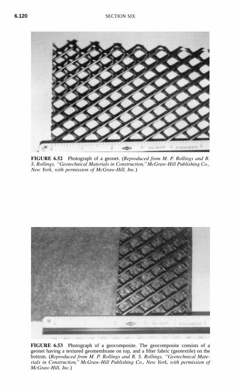
6.120 SECTION SIX
FIGURE 6.52 Photograph of a geonet. (Reproduced from M. P. Rollings and R.S. Rollings, ‘‘Geotechnical Materials in Construction,’’ McGraw-Hill Publishing Co.,New York, with permission of McGraw-Hill, Inc.)
FIGURE 6.53 Photograph of a geocomposite. The geocomposite consists of ageonet having a textured geomembrane on top, and a filter fabric (geotextile) on thebottom. (Reproduced from M. P. Rollings and R. S. Rollings, ‘‘Geotechnical Mate-rials in Construction,’’ McGraw-Hill Publishing Co., New York, with permission ofMcGraw-Hill, Inc.)
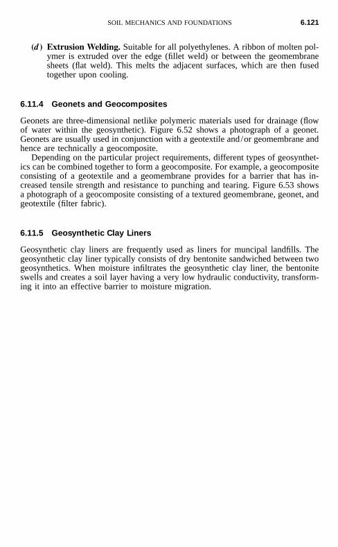
SOIL MECHANICS AND FOUNDATIONS 6.121
(d ) Extrusion Welding. Suitable for all polyethylenes. A ribbon of molten pol-ymer is extruded over the edge (fillet weld) or between the geomembranesheets (flat weld). This melts the adjacent surfaces, which are then fusedtogether upon cooling.
6.11.4 Geonets and Geocomposites
Geonets are three-dimensional netlike polymeric materials used for drainage (flowof water within the geosynthetic). Figure 6.52 shows a photograph of a geonet.Geonets are usually used in conjunction with a geotextile and/or geomembrane andhence are technically a geocomposite.
Depending on the particular project requirements, different types of geosynthet-ics can be combined together to form a geocomposite. For example, a geocompositeconsisting of a geotextile and a geomembrane provides for a barrier that has in-creased tensile strength and resistance to punching and tearing. Figure 6.53 showsa photograph of a geocomposite consisting of a textured geomembrane, geonet, andgeotextile (filter fabric).
6.11.5 Geosynthetic Clay Liners
Geosynthetic clay liners are frequently used as liners for muncipal landfills. Thegeosynthetic clay liner typically consists of dry bentonite sandwiched between twogeosynthetics. When moisture infiltrates the geosynthetic clay liner, the bentoniteswells and creates a soil layer having a very low hydraulic conductivity, transform-ing it into an effective barrier to moisture migration.