Section II

Descriptive Statistics

for continuous & binary Data

(including survival

data)

II - Checklist of summary statistics

Do you know what all of the following are and what they are for?

One variable – continuous data (variables like age, weight, serum levels, IQ, days to relapse ) _

Means (Y) Medians = 50th percentile Mode = most frequently occurring value Quartile – Q1=25th percentile, Q2= 50th percentile, Q3=75th percentile) Percentile Range (max – min) IQR – Interquartile range = Q3 – Q1 SD – standard deviation (most useful when data are Gaussian) (note, for a rough approximation, SD 0.75 IQR, IQR 1.33 SD) Survival curve = life table CDF = Cumulative dist function = 1 – survival curve Hazard rate (death rate) One variable discrete data (diseased yes or no, gender, diagnosis category, alive/dead) Risk = proportion = P = (Odds/(1+Odds)) Odds = P/(1-P) Relation between two (or more) continuous variables (Y vs X) Correlation coefficient (r) Intercept = b0 = value of Y when X is zero Slope = regression coefficient = b, in units of Y/X Multiple regression coefficient (bi) from a regression equation: Y = b0 + b1X1 + b2X2 + … + bkXk + error Relation between two (or more) discrete variables Risk ratio = relative risk = RR and log risk ratio Odds ratio (OR) and log odds ratio Logistic regression coefficient (=log odds ratio) from a logistic regression equation: ln(P/1-P)) = b0 + b1X1 + b2X2 + … + bkXk Relation between continuous outcome and discrete predictor Analysis of variance = comparing means Evaluating medical tests – where the test is positive or negative for a disease In those with disease: Sensitivity = 1 – false negative proportion In those without disease: Specificity = 1- false positive proportion ROC curve – plot of sensitivity versus false positive (1-specificity) – used to find best cutoff value of a continuously valued measurement

DESCRIPTIVE STATISTICS A few definitions: Nominal data come as unordered categories such as gender and color. Ordinal data come as ordered categories such as cancer stage, APGAR score, rating scales Continuous data (also called interval or ratio data) are measured on a continuum. Examples are age, weight, number of caries or serum bilirubin level. OUTLINE of the descriptive statistics for univariate continuous data A. Measures of central tendency (where the middle is) Mean, Median, Mode, Geometric mean (GM) B. Picturing distributions Histogram, cumulative distribution curve (CDF), "survival" curve, box and whisker plot, skewness C. Measures of location other then the middle Quartiles, Quintiles, Declines, Percentiles D. Measures of dispersion or spread Range, interquartile range (IQR), Standard deviation (SD) (note: Do not confuse an SD with a standard error or SE)

Measures of central tendency (where the middle is) In the examples below, we use survival times (in days) of 13 stomach cancer first controls (Cameron and Pauling, Proc Nat. Aca. Sci. Oct 1976, V 73, No 10, p 3685-3689). Times are from end of treatment (Tx) to death and are sorted in order. We use this data to illustrate definitions. 4, 6, 8, 8, 12, 14, 15, 17, 19, 22, 24, 34, 45. (n=13) Definintions: Mean = 4 + 6 + 8 + ... + 45 = 17.54 days = Y 13 Median = the middle value in sorted order. In this example, the median is the 7th observation = 15 days. Formally, the median is Y(7) = 15 days where Y(k) is the kth ordered value (Let n= sample size. For medians, if n is odd, take the middle value, if n is even, take the average of the two middle values). Mode = most frequency occurring value. It is 8 in this example. The mode is not a good measure in small samples and may not be unique even in large samples. Geometric mean (GM)= n(Y1 Y2 … Yn)= 134x6x8 x … 45 = 14.25 days If Xi=log(Yi), the antilog of X, or 10X, is the GM of theYs. That is, log GM = log(Yi) or GM = 10 ( log(Yi) )/n n The GM is always less than or equal the usual (arithmetic) mean. (GM arithmetic mean). If the data is symmetric on the log scale, the GM of the Ys will be about the same as the median Y. Note the similarity between the median and the geometric mean (GM) in this example. For survival data, the median and geometric mean are often similar. If we drop the longest survivor (45 days), note that now Mean = Y=15.25 days Median = (Y(6) + Y(7))/2 = 14.5 Geometric mean (GM) = 13.0 The (arithmetic) mean changes more than the median or the geometric mean when an extreme value is removed. The median (and often the GM) is said to be more “robust” to changes than the mean.

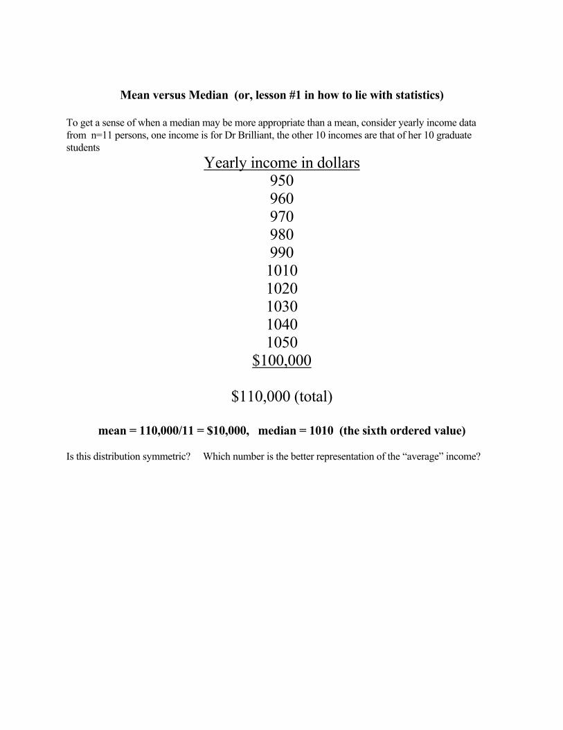
Mean versus Median (or, lesson #1 in how to lie with statistics)

To get a sense of when a median may be more appropriate than a mean, consider yearly income data from n=11 persons, one income is for Dr Brilliant, the other 10 incomes are that of her 10 graduate students

Yearly income in dollars 950 960 970 980 990 1010 1020 1030 1040 1050

$100,000

$110,000 (total)

mean = 110,000/11 = $10,000, median = 1010 (the sixth ordered value) Is this distribution symmetric? Which number is the better representation of the “average” income?

Mean versus Median when the data are censored (topic may be omitted) Sometimes the actual data value is not observed, only a minimum or floor of the true value. When such a minimum of the true value is observed, the observed value is called censored. By far the most common example involves time from diagnosis (or treatment) to death. If a subject is still alive, the true time of death is not observed. We only have a lower bound, the time from diagnosis (or treatment) to the last follow up. In the case of censored data, the mean may not be the best measure of typical behavior or central tendency. Example - Survival times in women with advanced Breast Cancer Below are survival times in days in a group of n=16 women. The data in the left column was collected after 275 days of follow-up. The data in the right column, on the same 16 women, was collected after 305 days of follow-up. Survival time in days after end of radiotherapy woman after 275 days f/u after 305 days f/u 1 14 14 2 26 26 3 43 43 4 45 45 5 50 50 6 58 58 7 60 60 8 62 62 9 70 70 10 70 70 11 83 83 12 98* 128* 13 104* 134* 14 124* 154* 15 125* 155* 16 275* 305* mean 75.6 83.1 median 66.0 66.0 SD 55.8 66.3 *still alive (censored) The median is still a valid measure when less than half the data are censored. Questions: What if a patient dies of an unrelated cause? (i.e. is hit by a truck and dies?) Is the SD a good measure here? What if there is no censoring?

Data distributions and survival curves Consider this example using our stomach cancer data: Cumulative frequencies and survival Days num dead pct dead cum num dead cum pct dead cum pct alive=S 1-10 4 30.8 4 30.8 69.2 11-20 5 38.5 9 69.2 30.8 21-30 2 15.4 11 84.6 15.4 31-40 1 7.7 12 92.3 7.7 41-50 1 7.7 13 100.0 0 total 13 The cumulative frequency table or cumulative incidence (also called cumulative frequency distribution-CDF) is a further extension of the frequency distribution idea. It is a plot of the cumulative frequency versus time. The fourth and fifth columns from the left give the number (or percentage) who died in the current class interval plus all intervals proceeding. From this it is easy to see that the median survival time (discussed below) must be somewhere between 11 and 20 days. The rightmost column (Cumulative percent alive) is obtained from the previous column by subtracting the previous column's value from 100 percent. A plot of the values in the rightmost column versus survival time is called a Survival Curve (S curve) and is frequently cited when time to death or time to recurrence of a disease is being studied. The above method of obtaining the CDF and S curves based on class intervals of fixed length (i.e. 10 days) is called the actuarial method. Another method which provides a value at each death (or at each observation) is called the product-limit or Kaplan_meier method. Despite its imposing name, the product limit method just says that, the CDF =cumulative incidence= number of deaths up to time t / n where n is the sample size. The survival curve S at any time t (or at any observation x) is given by S = 1 - CDF = (n - number of deaths up to time t) /n Of course, we can make these curves with any data, not just survival data. (There is a complication that we will not discuss in depth. This involves producing a CDF or survival curve when persons have died of other causes, are lost to follow up or are still alive. Such persons are called censored, that is, the person is still alive and only the time till the last follow up is known.)

For the stomach cancer survival data we compute cumulate incidence and Survival = 1-cum incidence. t cumulative # <=t incidence Surv=S 4 1 .077 .923 6 2 .154 .846 8 4 .308 .692 12 5 .385 .615 14 6 .461 .538 15 7 .538 .461 17 8 .615 .385 19 9 .692 .308 22 10 .769 .231 24 11 .846 .154 34 12 .923 .077 45 13 1.000 .000

The numbers in the incidence column also indicate the cumulative percentiles. In this example, we would say that 34 is the 92nd percentile since 92% of the survival times are 34 or less.

Bevacizumab & Ovarian Cancer Berger et.a. NDJM Dec 2011

Why survival curves? Why should we insist on comparing survival curves and not just look at, for example, the percentage alive at some particular time such as one year or five years? The time one chooses to compare survival can give misleading impressions. At time zero, everyone is alive. After a long time, everyone eventually is dead. Therefore, if one wants to manipulate a comparison, one can choose to compare survival only at a time that supports whatever claim one wants to make. It is therefore better to demand to see an entire survival curve rather than the survival at a single point in time, particularly when making comparisons.

0%

10%

20%

30%

40%

50%

60%

70%

80%

90%

100%

0 1 2 3 4 5 6 7 8 9 10

day

pct

aliv

e

Summarizing mortality – hazard rates

Sometimes it is desirable to give a single summary (similar to a mean) in order to summarize mortality over time. A single summary that takes into account differing follow up in each person is the hazard rate. In the case where the outcome is death, this is also called the mortality rate. However, the term

hazard rate is used when the outcome is something other than death, such as disease occurrence.

Hazard rate = h = number of persons who had the outcome Total person-time follow up in all persons at risk

Note that this is a rate, per person-time. It is NOT a probability (not a risk).

In our stomach cancer survival time example with 13 persons, the total follow up is

4+6+8+8+12+14+15+17+19+22+24+34+45 = 228 person-days

There were, sadly, 13 deaths.

So the hazard rate (or, in this case, the mortality rate) is

Hazard rate = 13/228 = 0.057 or 5.7 deaths per 100 person-days of follow up.

The value of 0.057 does NOT say that one has a 5.7% chance of dying.

Ratios of these rates are often made when comparing one group to another.

It is more fair to compute hazard rates than to simply compute the percentage of persons who died. Simply computing the percentage ignores the follow up time.

Example:

Imagine that 100 persons receiving treatment A are compared to 100 similar persons receiving treatment B. In group A, seven have died and in group B, only 2 have died. One might be tempted to say that treatment B is better than A since only 2% of those who received B died compared to 7% who received A. However, if we also found that the mean follow up time is 36 months under treatment A and only 3 months under treatment B, then hazard rates are 7/( 36 x100) = 1.94 deaths per 1000 person-months for Treatment A and 2/( 3 x 100) = 6.66 deaths per 1000 person-months for Treatment B So, the rate of mortality is higher for B than for A even though the number of persons in each group is the same and more died in group A. The(hazard) rate ratio for A/B is 1.94/6.66=0.291. This is not to be confused with a risk ratio but is qualitatively similar. When ALL patients are followed to the endpoint, (no censoring) mean time to event= 1/hazard. (Also see the discussion about the Poisson distribution in Section III)

Hazard rates and survival curves

The hazard rate and survival curves have a direct relationship. The usual survival curve is a plot of Survival=S versus time (t). However, if the relation between loge(S) and t is linear, it fits the equation Y = a + h X where Y=loge(S) and X=t. In this equation, the intercept “a” is always zero since a is the value of loge(S)=1 when t=0. (When t=0, S=1 and log(S)=0 so a=0). Therefore, for survival, if the relation between loge(S) and t is linear, then loge(S) =-h t. The constant “h” is the hazard rate. (Equation assumes h is constant). Therefore, when the relation between loge(S) and t is approximately linear, the hazard rate h can also be interpreted as the average rate at which loge(S) is decreasing per unit time. For example, if t is in months, h is the rate of change of loge(S) per month.

Survival

0%

20%

40%

60%

80%

100%

0 2 4 6 8 10 12

t

S 0.2 0.4

hazard rate

log Survival

-6.0

-5.0

-4.0

-3.0

-2.0

-1.0

0.0

0 2 4 6 8 10 12t

log

(S)

0.2 0.4

hazard rate

When all subjects are followed to the endpoint (ie all patient followed till they die), the mean time to outcome = 1/hazard rate = 1/h. But if some have not reached the outcome (censored data), then this is NOT true and it is better to quote hazard rates, not means.

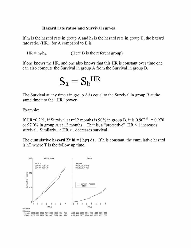
Hazard rate ratios and Survival curves If ha is the hazard rate in group A and hb is the hazard rate in group B, the hazard rate ratio, (HR) for A compared to B is HR = ha/hb. (Here B is the referent group). If one knows the HR, and one also knows that this HR is constant over time one can also compute the Survival in group A from the Survival in group B.

Sa = SbHR

The Survival at any time t in group A is equal to the Survival in group B at the same time t to the “HR” power. Example: If HR=0.291, if Survival at t=12 months is 90% in group B, it is 0.900.291 = 0.970 or 97.0% in group A at 12 months. That is, a “protective” HR < 1 increases survival. Similarly, a HR >1 decreases survival. The cumulative hazard Σt hi = ∫ h(t) dt . If h is constant, the cumulative hazard is hT where T is the follow up time.

Skewness

Another important property of distributions is the distribution symmetry or skewness. The mean is only in the middle when a distribution is symmetric. When the distribution is symmetric, the mean and the median are the same. The more skewed the distribution, the more the mean and median will differ. Long right tailed distribution median < mean (very common for survival data)

Long left tailed distribution median > mean (not as common in medicine)

Symmetric distribution median = mean (very common in medicine, sometimes on a log scale)

When continuous data is skewed, one must use “non parametric” statistical methods and quote medians rather than means.

Example: ICU length of stay

0

1

0 9

m e d ia n

m e a n

0 .0 0

0 .4 0

-3 .5 3 .5

0

1

0 9

m e d ia n

m e a n

mean

median

n=94, Mean=11.3 days, median = 6 days, range 1-80 days

Other measure of location and

MEASURES OF VARIABILITY (SPREAD) So far we have concentrated on measures of average or typical values. Another measure of "location" is the percentile, defined below. Differences between percentiles allow one to define measures of variability or spread. The range and interquartile range are two such measures. In order to define the interquartile range, we must first define a percentile. Imagine that the data is sorted from smallest to largest. The kth percentile is the data value X such that k% of the observations are lower than X and 100 - k% are higher than X. By definition, the first or lower quartile is the 25th percentile. That is, it is the data value X such that 25% of the observations are lower than X and 75% are higher. This value is often denoted Q1 for first quartile. The third or upper quartile is the 75th percentile (Q3). The second quartile is the median. Of course, this grouping into "bins" containing 25% of the observations is arbitrary. When the data is grouped into 20% bins, (20th, 40th, 60th, 80th and 100th percentiles) the boundary values are called quintiles. When the data is grouped into 10% bins the values are called deciles.

'

6 18 30 42 54 66 78

0

10

20

30

40

50

60

70

80P

erce

nt

LOS_ICU

0

0.1

0.2

0.3

0.4

0.5

0 2 4 6 8 10 12 14 16 18 20

Q1 Q3median

25% 25%25% 25%

The interquartile range and the box plot

The distance between the 1st and 3rd quartiles is defined as the interquartile range. This is the range that captures the middle 50% of the data. Let Q1 = lower quartile Q3 = upper quartile, then IQR = interquartile range = Q3 - Q1. Below is a graphical display called a box and whisker plot (or sometimes just a box plot) that summarizes a distribution of some measurement X. A star (*) is often used to indicate the position of the mean. +-------------------+ | | | minimum ----------------| | * +-------maximum | | | +-------------------+ Q1 median Q3 _________________________________________________________________ scale of X In this plot, the IQR is indicated by the inside of the box.

mean

The Variance and the Standard Deviation

Another measure of spread is defined by a rather complicated looking formula. If there are n observations, if Xi is the ith data value and X is the mean, then the (sample) variance is defined as _ Variance = (Xi - X)2 (n-1) In words, the variance is the average squared deviation from the mean. Note, however, that we divide the sum of squared deviations from the mean by n-1, not by n. If X is in units of years, then the units of the variance is "squared" years. Therefore, variances are not usually reported in the medical literature. What is reported is the standard deviation or SD. By definition, the (sample) standard deviation is the square root of the variance. SD = Variance The SD is in the original units of X. The symbol S is also often used instead of SD for the standard deviation. Another name for the SD, used by engineers, is the average RMS (root-mean square) deviation (from the mean). At first glance, the SD is not an intuitive measure of variation. However, when the data distribution is unimodal, symmetric and "bell shaped", that is, when the data is well approximated by a Normal or Gaussian distribution (discussed later), the SD turns out to be a reasonable way to summarize the variability. Useful rules of thumb and the “normal” clinical range When the data distribution is unimodal symmetric & bell shaped, we will learn later that, approximately the middle 2/3 of the data are in the range: mean +/- SD the middle 95% of the data are in the range: mean +/- 2SD The second rule implies that the range of the data is approximately 4SD. Therefore, for unimodel, symmetric distributions, SD approximately equals range (for "small" samples). 4 In clinical practice, when data is gathered on disease free ("normal") individuals, the mean +/- 2S rule is often used to establish (at least provisionally) a normal clinical range. One must have a sense of the normal range of a parameter in order to know when an individual is diseased and when "outliers" are present.

Computing the variance and standard deviation (SD) For our stomach cancer survival data, the variance can be computed “manually” as shown below. This can be avoided if one uses a calculator or spreadsheet with a built in SD function. (STDEV in EXCEL, for example) Data 4,6,8,8,12,14,15,17,19,22,24,34,45 (n=13) Mean = 17.54 days, _ _ X X-X (X-X)2 4 -13.54 183.3 6 -11.54 133.2 8 -9.54 91.0 8 -9.54 91.0 12 -5.54 30.7 14 -3.54 12.5 15 -2.54 6.5 17 -0.54 0.3 19 1.46 2.1 22 4.46 19.9 24 6.46 41.7 34 16.46 270.9 45 27.46 754.1 sum 0 1637.2 variance = 1637.2/12 = 136.4 days2 SD = standard deviation = 136.4 = 11.7 days Note that the lower quartile (Q1) is 8 days and the upper quartile (Q3) is 22 days. The interquartile range, another measure of variation, is 22-8 = 14 days. It is not necessarily the same as the SD.

Computing the Standard Deviation of Differences – paired data

The example below shows that the SD of a set of “end” minus “start” differences is not related in a simple way to the SD of the “start” data or the SD of the “end” data. The table below shows serum cholesterol (chol) in mmol/L from 6 patients who were put on a regimen of superactivated charcoal. They consumed the charcoal after every breakfast and dinner for three weeks. Their cholesterol at the start and end of the regimen is recorded. person chol at start chol at end decline (difference) 1 12.6 10.0 2.6 2 8.5 7.5 1.0 3 7.0 5.8 1.2 4 6.9 4.9 2.0 5 5.8 4.0 1.8 6 4.1 3.8 0.3 mean 7.48 6.00 1.48 SD 2.90 2.38 0.82 Imagine that only the "start" and "end" statistics were reported as in the box above. (mean=7.48 at start, SD=2.90 at start. mean=6.00 at end, SD=2.38 at end). From these statistics we can reconstruct the correct mean difference. That is, the mean difference is 7.48 mmol/L – 6.00 mmol/L = 1.48 mmol/L So, the difference of the means = the mean of the differences. But this rule does NOT work with the standard deviations. Note that 2.90 mmol/L - 2.38 mmol/L = 0.52 mmol/L. But the SD of the differences is 0.82 mmol/L. In general, the SD of the differences also depends on the correlation (r) between the start and end values, not just the starting SD and the ending SD. In this data, r= 0.971. (SDdifference= √ [SD2

start + SD2end – r 2 SDstart SDend] )

For treatment efficacy, the most relevant SD is often the SD of the differences, not the starting SD or the ending SD. The mean difference of 1.48 mmol/L tells us, on average, how effective the treatment is. On average, patients cholesterol declined 1.48 mmol/L. The SD of the differences, the 0.82 mmol/L, is a measure of how patients vary in their response as opposed to how much they vary at the start (or the end). A related question: If all six subjects had a cholesterol decrease of 2.0 mmol/L, what would be the SD of the differences?

Computing the SD of differences (& sums) – unpaired independent groups

For comparing age between two groups (A and B), the table below gives some summary statistics.

Ages in group A (n=4) and group B (n=3) group A group B 30 50

35 51 77 55 41

n 4 3 B – A B + A

mean 45.75 52.00 6.25 97.75 SD 18.46 2.16 18.58 18.58

Var=SD2 340.69 4.67 345.35 345.35 It is clear that the mean difference for B – A is 52.00 – 45.75 = 6.25. The formula above can also be applied to obtain the SD of 18.46 in group A and SD of 2.16 in group B. But what is the SD of the differences B-A? This is NOT a paired comparison but a comparison of two independent groups. The tables below give the differences and sums for ALL 4 x 3 = 12 possible pairwise combinations/ comparisons between the two groups and their means, SDs and variances (n=12).

All possible differences, B-A all possible sums, B+A 50 51 55 50 51 55

30 20 21 25 30 80 81 85 35 15 16 20 35 85 86 90 77 -27 -26 -22 77 127 128 132 41 9 10 14 41 91 92 96

mean 6.25 mean 97.75 SD 18.58 SD 18.58 Var 345.36 Var 345.36

In this calculation, the variances of B-A and the variances of B+A are the same. Moreover, 345.36 = 340.69 + 4.67. That is,

Var(Y - X) = Var(Y) + Var(X) Var(Y + X) = Var(Y) + Var(X) SD(Y-X) SD(Y-X)= √ SD2(Y) + SD2(X) SD(Y) SD(Y+X)=√ SD2(Y) + SD2(X)

SD(X)

Section II (cont)

Statistics for bivariate binary data (2 x 2 tables) Very often we look at binary nominal or categorical data. Male and female, alive or dead, diseased or well are all examples of binary nominal categories. Two important statistics for describing the relationship between two binary variables are the relative risk (RR) and the odds ratio (OR). The RR and OR are often employed in epidemiology when we wish to quantify the risk of disease in those exposed to a possible causative agent compared to those not exposed to the agent. This also applies to experimental trials where we compare those still not cured in those “exposed” to a new treatment compared to those on a standard treatment. Discrete data frequency counts are often arranged in a 2x2 table

Diseased Non Diseased Total Exposed (e) a b a+b

Unexposed (u) c d c+d

Relative risk or risk ratio and prospective studies In a prospective study, we can think of this table as being composed of two groups, the exposed group of a+b persons and the unexposed group of c+d persons. The risk of disease in the exposed group is defined as Pe = risk = a/(a+b). This is the proportion (P) with the disease. Similarly, in the unexposed group, the risk of disease is Pu= c/(c+d). Obviously, the risk ratio or relative risk in the exposed versus the unexposed is defined by risk in exposed/risk in unexposed = (a/(a+b))/(c/(c+d)) = Pe/Pu = a(c+d) = risk ratio = relative risk = RR c(a+b) It is also important to report the risk difference, Pe-Pu as well as the risk ratio. For a rare disease where Pu = 1/100,000 in unexposed, even if the risk ratio is RR=10, Pe is still only 1/10,000, still a rare event. It is misleading to report only the risk ratio.

Odds, Odds ratio and retrospective (case-control) studies

If “a” persons have disease and “b” persons do not have disease in a group of a+b persons, then P=a/(a+b) is the risk of disease. The odds of disease is defined as O = a/b. For example, if a=10 have disease and b=90 do not, then a+b=100, the risk= 10/100 = 0.10 and the odds = 10/90 = 0.11. In general, O= odds = risk/(1-risk) = P/(1-P) and P= risk = odds/(odds + 1)= O/(O+1) In ordinary language, one says that the risk is 10% (1 in 10) or the odds is 1 to 9. Risk is the ratio of diseased persons to all persons. Odds is the ratio of those with disease to those without disease. Of course, if a/b is the odds of disease in the exposed group and c/d is the odds of disease in the unexposed group, then the odds ratio is, by definition odds ratio = OR = Oe/Ou= (a/b)/(c/d) = ad/bc. When there is no association between exposure and disease both the relative risk and the odds ratio are equal to 1.0. (and their logarithms are equal to zero). Moreover, when a disease is rare, so that a and c are small relative to b and c, the OR is approximately equal to the RR. For example, consider the table below. Diseased Not Diseased total Exposed 50 950 1000 Unexposed 200 8550 8750 RR = (50/1000)/ (200/8750) = 2.188, OR = (50/950)/ (200/8550) = 2.25 Why quote odds ratios when we can quote relative risks? The odds ratio, ad/bc, is the odds of disease in the exposed relative to the unexposed. However, the odds ratio is also the odds of exposure in the diseased (cases) versus the not diseased (controls)! Unlike the RR, the OR comes out the same regardless of which variable is the exposure variable and which is the outcome variable. As shown in the above example, when the disease is rare, the OR approximates the RR. Therefore, when the disease is rare, the OR of exposure in a retrospective, case control study can be used to get an estimate of the RR of disease in a prospective study!! This is not intuitive since it is not possible to obtain the absolute risk of disease in a case control study. However, to the degree that the OR approximates the RR, it is possible to estimate the relative risk of disease by looking at the odds ratio for exposure in diseased versus non diseased groups (which equals the odds ratio of disease in exposed versus non exposed groups). This is one of the chief reasons why case-control studies are valuable (and why they can also be very misleading). If one knows the absolute risk of disease in the unexposed population, Pu, then one can compute the RR from the OR by RR = OR/(1 – Pu + OR Pu).

Why Odds Ratios (OR) are the same in a prospective and retrospective study – an example

PROSPECTIVE STUDY & POPULATION

BC no BC Total risk odds

OC 50 950 1000 0.050 0.053 no OC 200 8550 8750 0.0228 0.0234

OC use 0.2 0.1 RR OR

ratio 2.188 2.250

RETROSPECTIVE (Case control) STUDY BC=Breast Cancer

BC no BC OC=oral contraceptive use

OC 100 5 no OC 400 45

500 50

OC use 0.2 0.1

odds 0.25 0.11 OR 2.25

This example uses the data above and assumes that: 1. There is no confounding 2. There is no bias 3. For simplicity, the prospective sample is a random, representative sample of the population. In the prospective study above, the RR = 2.188 and the OR = 2.25. Further, in the prospective study, patients are chosen on the basis of their OC status. That is, the number of OC and non OC patients are fixed by the investigator, but the BC (breast cancer) frequencies are determined by nature. However, note that 20% of the BC patients use OCs and 10% of the non BC patients use OCs. Now, suppose we do a retrospective study, where the number of BC and non BC patients are determined by the investigator. Say, as an arbitrary example, we get 500 BC patients and 50 matched BC free controls. (The imbalance is deliberate to demonstrate that the sample size does not have to be the same). If sampling BC patients and non BC controls is indepdent of OC status, we expect that 20% of the BC patients will use OCs and that 10% of the non BC patients will use OCs. This will force the OR to be 2.25, just as in the prospective study. While the numerator and denominator odds are not the same in the prospective versus the retrospective studies, the ratio (that is the OR) is the same. Frequency data: disease status disease no disease exposed a b not exposed c d Prospective Retrospective both equal Odds Ratio a/b a/c = ad c/d b/d bc

Why use ORs? 1.In prospective studies, we usually quote disease risk & risk ratio (RR). In case-control, we always quote OR, not RR. Case-control OR of exposure in disease/no disease equals the prospective OR of disease in exposed/unexposed in the population if the probability of exposure is same as in the target population. (Not necessarily true if there is confounding, bias). 2. OR more “stable” (universal) across studies. If unexposed risk=20%, RR=2, exposed risk=40% If unexposed risk=60%, RR can’t be 2.

Independence/multiplication rule for Odds ratios

ORs for heart attack (MI) For smokers/non smoker: OR = 4 For alcohol/no alcohol: OR = 2

If the odds ratios for smoking and alcohol are independent, the OR for those who smoke AND drink alcohol is 4 x 2 = 8 (relative to no smoke,

no alcohol).

This “multiplication rule” is only true if smoking and drinking are independent influences on MI. In a study where both a measured, can

determine if the two factors are independent.

Having a logistic regression model that contains no interaction terms is equivalent to making the assumption of independence and therefore of multiplicity on the OR scale since it is an assumption of additivity on the log OR scale.

Other statistical definitions for binary outcomes NNT-Number needed to treat

When evaluating the benefit of a treatment in a clinical trial (experiment) where disease reduction (risk reduction) is desired, the following definitions are often encountered. Pc = Proportion (risk) with disease under the control (standard) treatment (like Pu) Pt = Proportion (risk) with disease after using the new treatment (like Pe) RR = Risk ratio = relative risk of disease = Pt/Pc (like Pe/Pu above) (Some report RR= Pc/Pt depending on context) Absolute risk reduction = ARR = Pc – Pt = risk difference = RD (The standard error for ARR is given in the confidence interval section of the notes) Relative risk reduction = RRR = (Pc – Pt)/ Pc = ARR/Pc = 1- (1/RR) Reduction relative to the control risk of disease NNT = number needed to treat = 1/ARR The NNT is the absolute number of patients that need to be treated with the new treatment in order to prevent (or cure) one (new) person with disease compared to control. Example: Pc = 0.36 = 36%, Pt = 0.34 = 34% ARR = RD= 0.36 – 0.34 = 0.02 = 2% RRR = 0.02/0.36 = 0.055 = 5.5%, RR= 0.34/0.36 = 0.944 (some report RR=0.36/0.34= 1.059 – must label clearly) NNT = 1/0.02 = 50 Thus, 50 patients must be given the new treatment to prevent (or cure) one additional disease case compared to the control treatment. The NNT is a common measure of the benefit to be obtained from a new treatment.

In the context of etiology, if Pu=1/10,000 and Pe=3/10,000, RD = 2/10,000 but RR=Pe/Pu = 3.0

Summary – “Ratios” For one group:

Risk Odds Hazard rate P O h

For comparing two groups (exposed=e vs unexposed=u)

Ratio: RR=Pe/Pu OR=Oe/Ou HR=he/hu

All of these ratios above have the null value of 1.0 when there is no association. The distribution of the logs of their ratios from study to study are usually bell curve shaped around the true population value. The log scale null value is log(1.0) = 0.

Sensitivity and Specificity in diagnostic tests 2x2 tables are also often used to present information concerning the evaluation of diagnostic tests. This sort of information should not be confused with the disease versus exposure information in the previous section. In evaluating a diagnostic test, one must have some way of determining the true state of a patient (diseased or not diseased). For example, one may have to wait until autopsy to obtain the definitive "gold standard" true diagnosis. Or, to obtain the true diagnosis, one might often have to perform invasive surgical procedures or use expensive technology. Therefore, there is often a great need for a simpler and/or cheaper diagnostic test to be used in place of the expensive or generally unavailable gold standard. However, in order to evaluate whether the diagnostic test is an adequate proxy for the definitive gold standard, both the sensitivity and specificity of the test must be high. The sensitivity of a test is defined as the proportion of all truly diseased persons who test positive. 1 - sensitivity is defined as the proportion of false negatives. The specificity of a test is defined as the proportion of all truly disease free persons who test negative. 1 - specificity is defined as the proportion of false positives. These definitions can be summarized in reference to the 2 x 2 table below.

“gold standard” True-disease True-no disease

Test positive a b Test negative c d

total a+c b+d Sensitivity = a/(a+c) False negative proportion = c/(a+c) Specificity = d/(b+d) False positive proportion = b/(b+d) Positive predictive value (PPV) = a/(a+b)* Negative predictive value (NPV) = d/(c+d)* * not a measure of test performance since it depends on disease prevalence . This definition is only appropriate if the data is from a prospective study where the overall prevalence is (a+c)/(a+b+c+d) = (a+c)/n

ROC curves – best continuous data cutpoint If we have a continuous variable Y (often a lab variable), we can choose a threshold (or cutoff), Yc, such that we designate a patient positive for disease if Y > Yc and designate a patient negative if Y < Yc.(or the reverse). But what is the best value for Yc? We can vary Yc, recompute the sensitivity and specificity, and graph the “tradeoff” between sensitivity and specificity, sometimes expressed as sensitivity versus (1-specificity)=false positive probability. Plots of sensitivity versus false positive or sensitivity and specificity on the same axis are examples of ROC curves.

0%

10%

20%

30%

40%

50%

60%

70%

80%

90%

100%

0.0 0.1 0.2 0.3 0.4 0.5 0.6 0.7 0.8 0.9 1.0

Yc =threshold (cutpoint)

sensitivity

specificity

0.00

0.10

0.20

0.30

0.40

0.50

0 0.1 0.2 0.3 0.4 0.5 0.6 0.7 0.8 0.9 1

Y

Y

If we define accuracy = (sensitivity + specificity)/2 we can plot accuracy versus the cutpoint Yc. (More generally, accuracy = W sensitivity + (1-W) specificity for 0 < W < 1. W represents the relative “weight” we give to sensitivity versus specificity. W=0.5 is unweighted accuracy).

accuracy

0%

10%

20%

30%

40%

50%

60%

70%

80%

90%

100%

0 0.1 0.2 0.3 0.4 0.5 0.6 0.7 0.8 0.9 1

Yc =threshold (cutpoint)

un

wei

gh

ed a

ccu

racy

One finds the cutpoint (threshold) that maximizes the accuracy. The highest accuracy does NOT necessarily occur where the sensitivity equals the specificity.

“Traditional” ROC curve C (concordance) statistic for ROC A measure of how accurate the variable Y can separate the disease and non disease groups is the concordance statistic, denoted C. C is the area under the “traditional” ROC curve above. The value of C ranges from 0.5 (bad) to 1.0 (perfect). Alternative interpretation of C - If there are nd=a+c true diseased subjects and nnd=b+d true not diseased subjects, imagine forming all nd x nnd pairs of subjects where one member of the pair has disease and the other does not. Also assume that the diseased patients have the larger values of Y, so we predict positive if Y>Yc. Call a given pair “concordant” if the diseased patient in the pair is positive and the non diseased patient is negative. Then C is the proportion of the pairs that are concordant.

traditional ROC

0%10%20%30%40%50%60%70%80%90%

100%

0% 10% 20% 30% 40% 50% 60% 70% 80% 90% 100%

false pos=1-spec

sen

s

Positive and Negative Predictive Values

In general, positive predictive value (PPV) and negative predictive value (NPV) depend on sensitivity (sens), specificity (spec) and the disease prevalence (P). In contrast, sensitivity and specificity do NOT depend on disease prevalence. If we compute PPV and NPV using PPV=a/(a+b) and NPV=d/(c+d) as above, this is only valid for a disease prevalence equal to

P = (a+c)/(a+b+c+d) = (a+c)/n

Bayes formulas for PPV and NPV

Let P = prevalence of disease

PPV = test true pos/ (test true pos + test false pos) = Sens x P / [ Sens x P + (1- Spec) x (1- P) ]

NPV = test true neg/ (test true neg + test false neg) = Spec x (1-P) / [ Spec x (1-P) + (1-Sens) x P ]

Example: Disease no disease Total

Test positive 95 20 115 Test negative 5 1980 1985

Total 100 2000 2100

Sens = 95/100=0.95, Spec= 1980/2000 = 0.99, P = 100/2100 = 0.0476

PPV = (0.95 x 0.0476) / [ 0.95 x 0.0476 + 0.01 x 0.9524 ] = 0.826 PPV = 95/115=0.826

NPV = (0.99 x 0.9524) / [0.99 x 0.9524 + 0.05 x 0.0476] = 0.9974 NPV = 1980/1985 = 0.9974 P is also sometimes called the “prior probability” of disease and the PPV is the “posterior” (post testing) probability of disease.

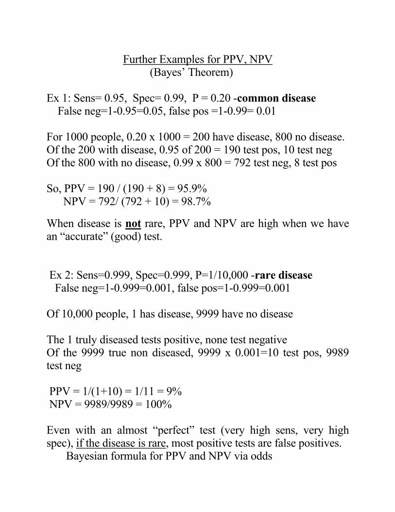
Further Examples for PPV, NPV (Bayes’ Theorem) Ex 1: Sens= 0.95, Spec= 0.99, P = 0.20 -common disease False neg=1-0.95=0.05, false pos =1-0.99= 0.01 For 1000 people, 0.20 x 1000 = 200 have disease, 800 no disease. Of the 200 with disease, 0.95 of 200 = 190 test pos, 10 test neg Of the 800 with no disease, 0.99 x 800 = 792 test neg, 8 test pos So, PPV = 190 / (190 + 8) = 95.9% NPV = 792/ (792 + 10) = 98.7%

When disease is not rare, PPV and NPV are high when we have an “accurate” (good) test. Ex 2: Sens=0.999, Spec=0.999, P=1/10,000 -rare disease False neg=1-0.999=0.001, false pos=1-0.999=0.001 Of 10,000 people, 1 has disease, 9999 have no disease The 1 truly diseased tests positive, none test negative Of the 9999 true non diseased, 9999 x 0.001=10 test pos, 9989 test neg PPV = 1/(1+10) = 1/11 = 9% NPV = 9989/9989 = 100% Even with an almost “perfect” test (very high sens, very high spec), if the disease is rare, most positive tests are false positives. Bayesian formula for PPV and NPV via odds

(“Bayesian paradigm”)

Computing the PPV or the NPV is a special case of a more general approach to computing probabilities from odds, the “Bayesian paradigm”. The general concept is that one has a “prior” probability of the event of interest (ie, having a disease) that is known before one has gathered any data. Then, once the data (in this example, the disease test result) has been obtained, the prior probability is updated. This updated probability is called the posterior probability. The posterior is also a conditional probability given the data (given the test result).

Prior probability -> data -> posterior probability

The relation between the prior probability and the posterior probability is via their corresponding odds and via the odds of the data (test result). This “odds of the data” is called the (data) likelihood ratio (LR) where LR = probability of the data (a positive test) given disease probability of the data (a positive test) given no disease LR = sensitivity/false positive = sensitivity/(1-specificity)

Once the data LR is known

Posterior odds of disease = prior odds of disease x data LR Using the data from the previous example

Prior disease probability=prevalence =100/2100=0.0476, Test sensitivity=95/100=0.95, test false positive=20/2000=0.01

Odds Probability Prior 100/2000=0.05 100/2100=0.0476=4.76%

LR (“data is a pos test”)

Sens/false pos= 0.95/0.01=95

(not applicable)

Posterior 0.05 x 95=4.75 4.75/(1+4.75)=0.826=82.6%

Summary - Univariate statistics for binary data

Risk of disease = num disease / total at risk = P (=”proportion”)

Odds of disease = num disease / num without disease = O

Summary -Bivariate statistics for binary data True diseased True not diseased total

test positive or e a b a+b test negative or u c d c+d

total a+c b+d n Define: “positive” = “exposed”=”e”, “negative = ‘unexposed”=”u”

Risk difference = RD (also called absolute risk reduction) Risk in positive – Risk in negatives= Ppos- Pneg = Pe - Pu

Risk ratio = relative risk = RR Risk in positive / Risk in negative = [a/(a+b)] / [c/(c+d)] = Ppos / Pneg = Pe /Pu

Odds ratio =OR= odds if exposed / odds if unexposed= Oe/Ou = (a/b) / (c/d) = ad/bc (OR ≈ RR only if disease is rare/ P is small in target population)

Relative Risk reduction = RRR= RD/Risk in negatives = (Ppos – Pneg) / Pneg = (Pe-Pu)/Pu

NNT = number needed to treat = 1/RD = 1/( Ppos - Pneg) Sensitivity = Prob positive test is diseased = a/(a+c) Specificity = Prob negative test if not diseased = d/(b+d) Accuracy= W Sensitivity + (1-W) Specificity (0 ≤ W ≤ 1)

Positive predictive value = Prob disease if positive test = a/(a+b)

Negative predictive value = Prob no disease if negative test = d/(c+d)