(Section 3.7: Implicit Differentiation) 3.7.1

SECTION 3.7: IMPLICIT DIFFERENTIATION

LEARNING OBJECTIVES

• Understand that an equation can “determine” many implicit functions.

• Perform Implicit Differentiation and obtain templates of differentiation rules built on basic rules such as the Chain Rule.

• Relate derivatives obtained from Implicit Differentiation to slopes of tangent lines to a graph, even if the graph fails the Vertical Line Test (VLT).

PART A: EXPLICIT vs. IMPLICIT DEFINITIONS OF FUNCTIONS

• The equation y = x +1 defines y explicitly as a function of x. If f x( ) = x +1, then f is the corresponding explicit function.

• The equation y − x = 1 defines y implicitly as a function of x.

y − x = 1 is equivalent to our first equation, y = x +1. However, it is not solved for y. y is “buried in” the equation. If f x( ) = x +1, then f is the corresponding implicit function. (Technically, if we restrict the domain of f , we get other implicit functions.)

• The equation x2 + y2 = 1 “determines” (a questionable term, but used by some

sources) many implicit functions f : if y = f x( ) , then the equation is satisfied.

•• The graph of x2 + y2 = 1 fails the Vertical Line Test (VLT), and solving

for y yields y = ± 1− x2 , in which y is not a well-defined function of x.

•• However, any non-empty part of the graph that passes the VLT corresponds to an implicit function – examples are f1 , f2 , and f3 below.

Graph of x2 + y2 = 1

Graph of y = f1 x( ), where f1 x( ) = 1− x2 Graph of y = f2 x( ) , where f2 x( ) = − 1− x2

Graph of y = f3 x( ) , where

f3 x( ) = 1− x2 , 0.5≤ x ≤ 0.8

− 1− x2 , x ≤ 0.4

⎧⎨⎪

⎩⎪

• x2 + y2 = −1, whose graph is empty, determines no implicit functions.

(Section 3.7: Implicit Differentiation) 3.7.2 PART B: IMPLICIT DIFFERENTIATION

• We assume that the equations in this section determine at least one implicit function f that is differentiable “where needed.” Here, y = f x( ) , but we can also

have h = s t( ) , etc.

• Notation. We assume that ′y = dy

dx= Dx y .

WARNING 1: ′y . The ′y notation can be ambiguous if we have many

variables, or if we are dealing with dydt

, say, instead of

dydx

. In Section 3.8,

we will often prefer Leibniz notation such as dydt

.

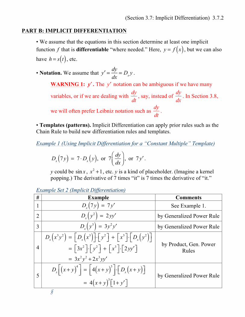
• Templates (patterns). Implicit Differentiation can apply prior rules such as the Chain Rule to build new differentiation rules and templates. Example 1 (Using Implicit Differentiation for a “Constant Multiple” Template)

Dx 7 y( ) = 7 ⋅Dx y( ), or 7

dydx

⎛⎝⎜

⎞⎠⎟

, or 7 ′y .

y could be sin x , x2 +1, etc. y is a kind of placeholder. (Imagine a kernel popping.) The derivative of 7 times “it” is 7 times the derivative of “it.”

Example Set 2 (Implicit Differentiation)

# Example Comments 1 Dx 7 y( ) = 7 ′y See Example 1.

2 Dx y2( ) = 2y ′y by Generalized Power Rule

3 Dx y3( ) = 3y2 ′y by Generalized Power Rule

4

Dx x3 y2( ) = Dx x3( )⎡⎣

⎤⎦ ⋅ y2⎡⎣ ⎤⎦ + x3⎡⎣ ⎤⎦ ⋅ Dx y2( )⎡

⎣⎤⎦

= 3x2⎡⎣ ⎤⎦ ⋅ y2⎡⎣ ⎤⎦ + x3⎡⎣ ⎤⎦ ⋅ 2y ′y⎡⎣ ⎤⎦= 3x2 y2 + 2x3 y ′y

by Product, Gen. Power

Rules

5

Dx x + y( )4⎡⎣⎢

⎤⎦⎥= 4 x + y( )3⎡

⎣⎢⎤⎦⎥⋅ Dx x + y( )⎡⎣ ⎤⎦

= 4 x + y( )31+ ′y⎡⎣ ⎤⎦

by Generalized Power Rule

§

(Section 3.7: Implicit Differentiation) 3.7.3

Example 3 (Implicit Differentiation)

Dx cos3 xy( )⎡⎣ ⎤⎦ = Dx cos xy( )⎡⎣ ⎤⎦3( ) Rewriting( )

= 3 cos xy( )⎡⎣ ⎤⎦2( ) ⋅ Dx cos xy( )⎡⎣ ⎤⎦( ) by Gen. Power Rule( )

= 3 cos xy( )⎡⎣ ⎤⎦2( ) ⋅ −sin xy( )⎡⎣ ⎤⎦ ⋅ Dx xy( )⎡⎣ ⎤⎦

by Gen. Trig Rules( )= 3 cos xy( )⎡⎣ ⎤⎦

2( ) ⋅ −sin xy( )⎡⎣ ⎤⎦ ⋅ Dx x( )⎡⎣ ⎤⎦ ⋅ y + x ⋅ Dx y( )⎡⎣ ⎤⎦( )by Product Rule( )

= 3 cos xy( )⎡⎣ ⎤⎦2( ) ⋅ −sin xy( )⎡⎣ ⎤⎦ ⋅ 1⋅ y + x ⋅ ′y( )

= −3 y + x ′y( ) cos2 xy( )⎡⎣ ⎤⎦sin xy( )

§

Example 4 (Using Implicit Differentiation to Find y’)

Consider the given equation x2 − 2x + y2 + 6y = 15 . Assume that it

“determines” implicit differentiable functions f such that

�

y = f x( ) .

Find a general formula for ′y , or

dydx

.

§ Solution

• If we solve for y by using Completing the Square (CTS), we obtain:

y = −3± 25− x −1( )2. (See Example 7.)

• Instead, Implicit Differentiation may be easier. Step 1. Implicitly differentiate both sides of the given equation with respect to x. We expect the result to include ′y .

x2 − 2x + y2 + 6y = 15 ⇒

Dx x2 − 2x + y2 + 6y( ) = Dx 15( )

WARNING 2: Write this last step. Otherwise, you are in danger of copying “15” instead of differentiating it! Very common error…

2x − 2+ 2y ′y + 6 ′y = 0

(Section 3.7: Implicit Differentiation) 3.7.4

Simplify by dividing both sides by 2.

x −1+ y ′y + 3 ′y = 0

Step 2. Isolate terms with ′y on one side.

y ′y + 3 ′y = 1− x

Step 3. Factor out ′y on that side.

′y y + 3( ) = 1− x

Step 4. Solve for ′y by dividing both sides by the other factor.

′y = 1− x

y + 3

Note 1: If we had not divided by 2 earlier, we would have had

′y = 2− 2x

2y + 6, which must be simplified to, say,

′y = 1− x

y + 3.

Note 2: Our formula for ′y includes y, itself! This allows us to analyze points on the graph of x

2 − 2x + y2 + 6y = 15 with the same x-coordinate but different y-coordinates (like “tiebreakers”). §

Example 5 (Evaluating y’; Revisiting Example 4)

Find the slope of the tangent line to the graph of x2 − 2x + y2 + 6y = 15

at the point 4,1( ) in the usual xy-plane.

§ Solution

Although it shouldn’t be necessary, we could check to ensure that the point

4,1( ) lies on the graph. We can plug in (substitute) x = 4 and y = 1 into the

equation to see if 4,1( ) is a solution point:

4( )2− 2 4( ) + 1( )2

+ 6 1( ) =?

15

15= 15 Checks( )

Therefore, 4,1( ) lies on the graph. (Let’s assume it’s not an endpoint.)

(Section 3.7: Implicit Differentiation) 3.7.5

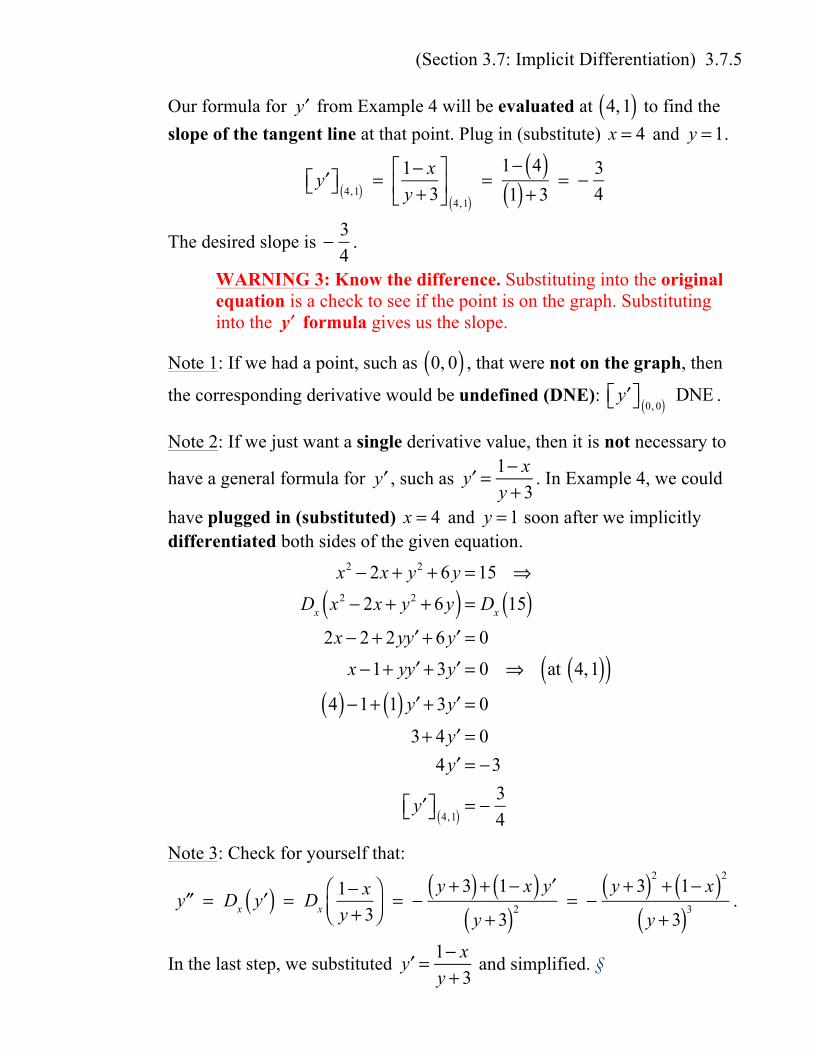
Our formula for ′y from Example 4 will be evaluated at 4,1( ) to find the slope of the tangent line at that point. Plug in (substitute) x = 4 and y = 1.

′y⎡⎣ ⎤⎦ 4,1( ) = 1− x

y + 3⎡

⎣⎢

⎤

⎦⎥

4,1( )=

1− 4( )1( ) + 3

= − 34

The desired slope is − 3

4.

WARNING 3: Know the difference. Substituting into the original equation is a check to see if the point is on the graph. Substituting into the ′y formula gives us the slope.

Note 1: If we had a point, such as 0, 0( ) , that were not on the graph, then

the corresponding derivative would be undefined (DNE):

′y⎡⎣ ⎤⎦ 0, 0( ) DNE .

Note 2: If we just want a single derivative value, then it is not necessary to

have a general formula for ′y , such as ′y = 1− x

y + 3. In Example 4, we could

have plugged in (substituted) x = 4 and y = 1 soon after we implicitly differentiated both sides of the given equation.

x2 − 2x + y2 + 6y = 15 ⇒

Dx x2 − 2x + y2 + 6y( ) = Dx 15( )2x − 2+ 2y ′y + 6 ′y = 0

x −1+ y ′y + 3 ′y = 0 ⇒ at 4,1( )( )4( )−1+ 1( ) ′y + 3 ′y = 0

3+ 4 ′y = 04 ′y = −3

′y⎡⎣ ⎤⎦ 4,1( ) = − 34

Note 3: Check for yourself that:

′′y = Dx ′y( ) = Dx

1− xy + 3

⎛⎝⎜

⎞⎠⎟= −

y + 3( ) + 1− x( ) ′y

y + 3( )2 = −y + 3( )2

+ 1− x( )2

y + 3( )3 .

In the last step, we substituted ′y = 1− x

y + 3 and simplified. §

(Section 3.7: Implicit Differentiation) 3.7.6

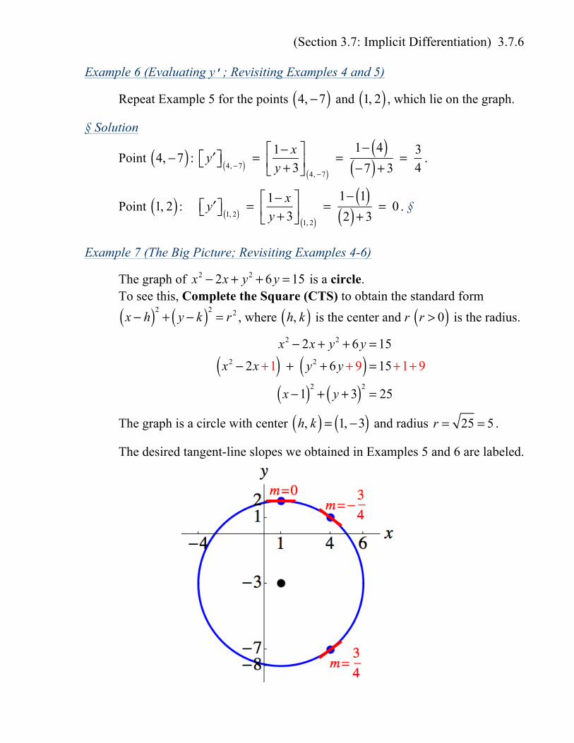
Example 6 (Evaluating y’; Revisiting Examples 4 and 5)

Repeat Example 5 for the points 4, −7( ) and 1, 2( ) , which lie on the graph.

§ Solution

Point 4, −7( ) :

′y⎡⎣ ⎤⎦ 4, −7( ) = 1− xy + 3

⎡

⎣⎢

⎤

⎦⎥

4, −7( )=

1− 4( )−7( ) + 3

= 34

.

Point 1, 2( ) :

′y⎡⎣ ⎤⎦ 1, 2( ) = 1− x

y + 3⎡

⎣⎢

⎤

⎦⎥

1, 2( )=

1− 1( )2( ) + 3

= 0 . §

Example 7 (The Big Picture; Revisiting Examples 4-6)

The graph of x2 − 2x + y2 + 6y = 15 is a circle.

To see this, Complete the Square (CTS) to obtain the standard form

x − h( )2+ y − k( )2

= r 2 , where h, k( ) is the center and r r > 0( ) is the radius.

x2 − 2x + y2 + 6y = 15

x2 − 2x +1( ) + y2 + 6y + 9( ) = 15+1+ 9

x −1( )2+ y + 3( )2

= 25

The graph is a circle with center h, k( ) = 1, −3( ) and radius r = 25 = 5 .

The desired tangent-line slopes we obtained in Examples 5 and 6 are labeled.

(Section 3.7: Implicit Differentiation) 3.7.7.

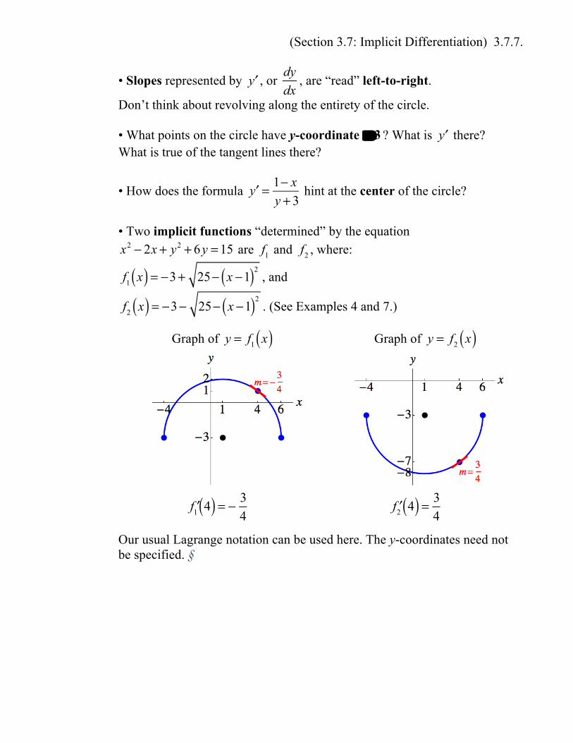
• Slopes represented by ′y , or

dydx

, are “read” left-to-right.

Don’t think about revolving along the entirety of the circle. • What points on the circle have y-coordinate − 3 ? What is ′y there? What is true of the tangent lines there?

• How does the formula ′y = 1− x

y + 3 hint at the center of the circle?

• Two implicit functions “determined” by the equation

x2 − 2x + y2 + 6y = 15 are f1 and f2 , where:

f1 x( ) = −3+ 25− x −1( )2, and

f2 x( ) = −3− 25− x −1( )2. (See Examples 4 and 7.)

Graph of y = f1 x( ) Graph of y = f2 x( )

′f1 4( ) = − 3

4

′f2 4( ) = 3

4

Our usual Lagrange notation can be used here. The y-coordinates need not be specified. §