secondary school - tripod.comsmktbr.tripod.com/file/ms-excel.pdfictl for secondary school programme...
TRANSCRIPT

KKEEMMEENNTTEERRIIAANN PPEELLAAJJAARRAANN MMAALLAAYYSSIIAA
SSeellff AAcccceessss LLeeaarrnniinngg MMoodduullee
MMiiccrroossoofftt EExxcceell
PUSAT PERKEMBANGAN KURIKULUM KEMENTERIAN PELAJARAN MALAYSIA
IIICCCTTT LLLiiittteeerrraaacccyyy fffooorrr SSSeeecccooonnndddaaarrryyy SSSccchhhoooooolll
PPPrrrooogggrrraaammmmmmeee
ICTL for Secondary School programme - Spreadsheet Module
1
MODULE 1
INTRODUCTION TO MICROSOFT EXCEL 2003
Curriculum Development Centre Ministry of Education Malaysia
ICTL for Secondary School programme - Spreadsheet Module
2
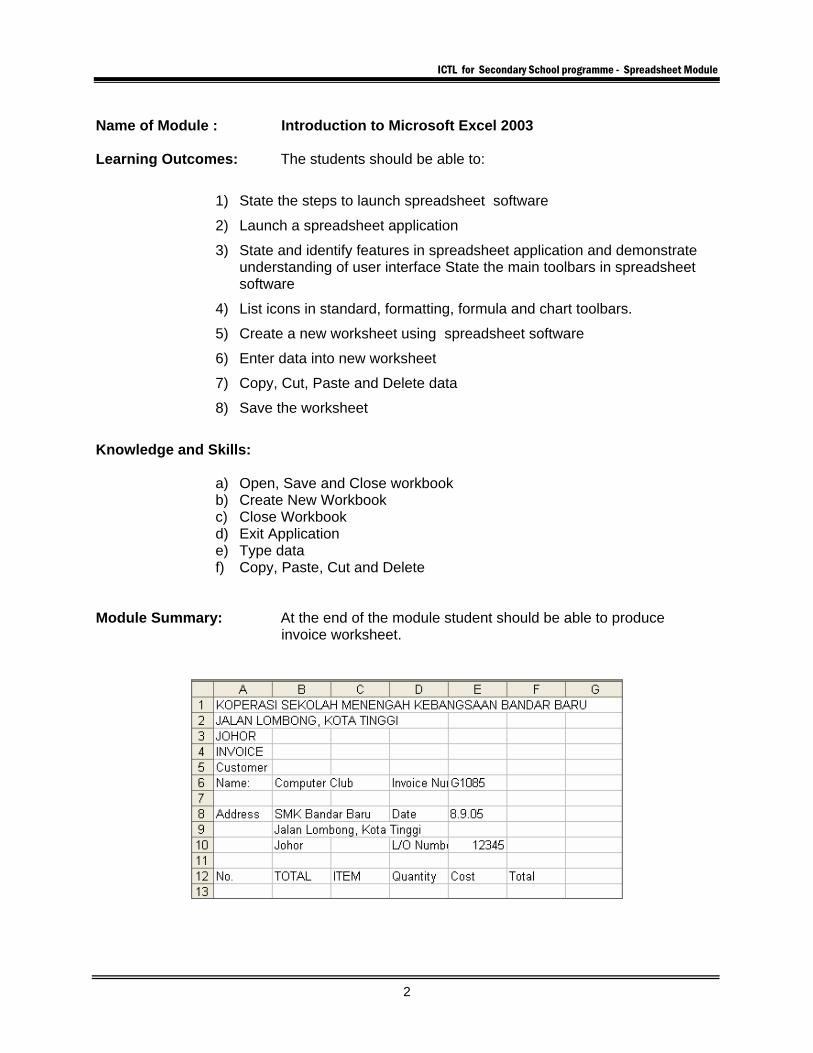
Name of Module : Introduction to Microsoft Excel 2003 Learning Outcomes: The students should be able to:
1) State the steps to launch spreadsheet software
2) Launch a spreadsheet application
3) State and identify features in spreadsheet application and demonstrate understanding of user interface State the main toolbars in spreadsheet software
4) List icons in standard, formatting, formula and chart toolbars.
5) Create a new worksheet using spreadsheet software
6) Enter data into new worksheet
7) Copy, Cut, Paste and Delete data
8) Save the worksheet
Knowledge and Skills:
a) Open, Save and Close workbook b) Create New Workbook c) Close Workbook d) Exit Application e) Type data f) Copy, Paste, Cut and Delete
Module Summary: At the end of the module student should be able to produce invoice worksheet.
ICTL for Secondary School programme - Spreadsheet Module
3
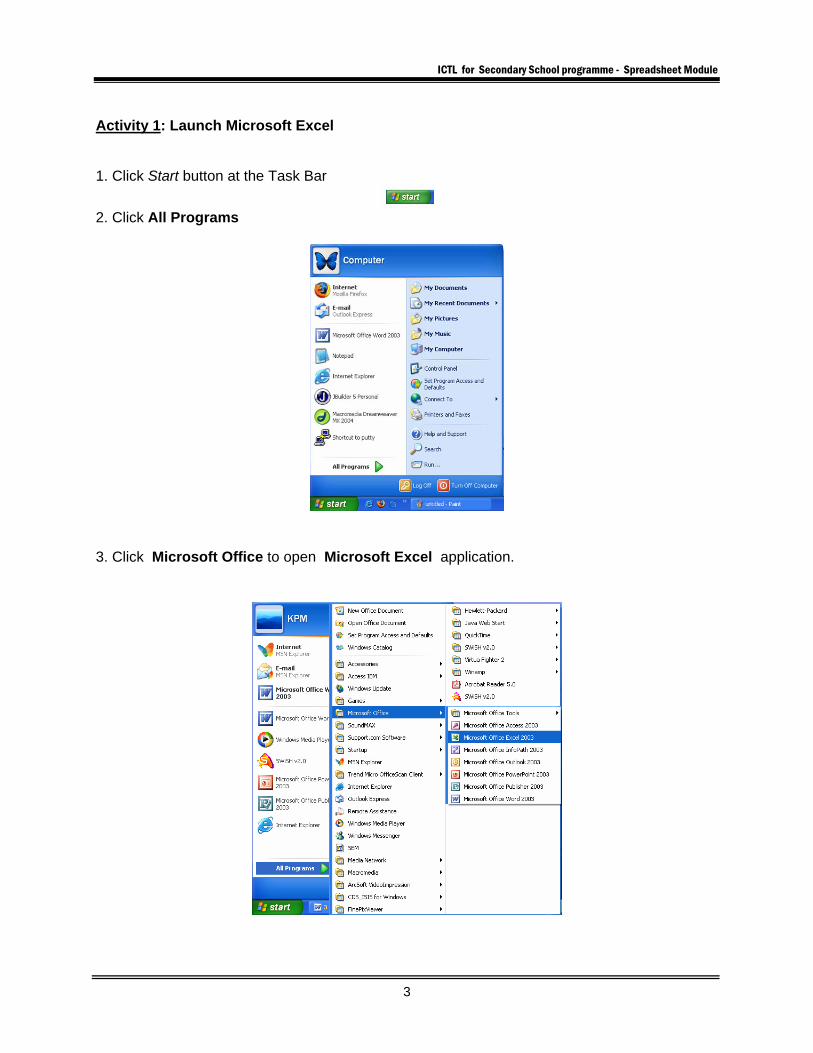
Activity 1: Launch Microsoft Excel 1. Click Start button at the Task Bar
2. Click All Programs
3. Click Microsoft Office to open Microsoft Excel application.
ICTL for Secondary School programme - Spreadsheet Module
4
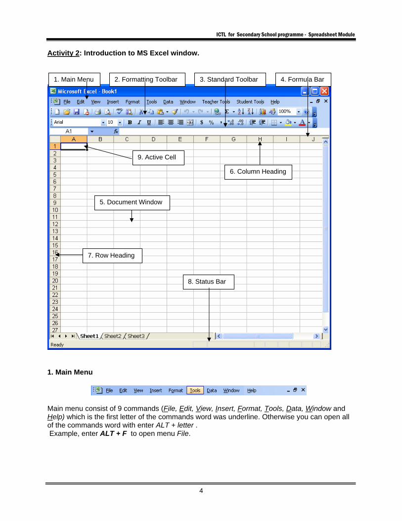
Activity 2: Introduction to MS Excel window.
1. Main Menu Main menu consist of 9 commands (File, Edit, View, Insert, Format, Tools, Data, Window and Help) which is the first letter of the commands word was underline. Otherwise you can open all of the commands word with enter ALT + letter . Example, enter ALT + F to open menu File.
1. Main Menu 2. Formatting Toolbar 3. Standard Toolbar 4. Formula Bar
9. Active Cell
5. Document Window
6. Column Heading
7. Row Heading
8. Status Bar
ICTL for Secondary School programme - Spreadsheet Module
5
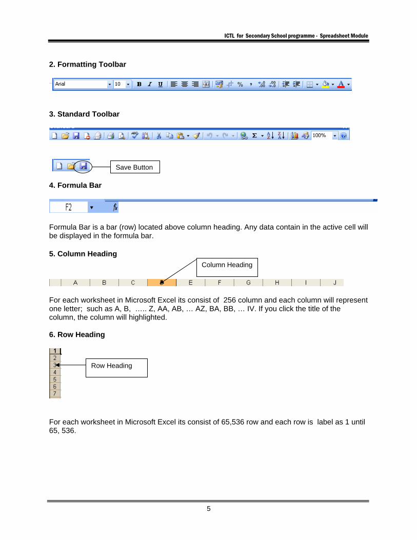
2. Formatting Toolbar
3. Standard Toolbar
4. Formula Bar
Formula Bar is a bar (row) located above column heading. Any data contain in the active cell will be displayed in the formula bar. 5. Column Heading
For each worksheet in Microsoft Excel its consist of 256 column and each column will represent one letter; such as A, B, ….. Z, AA, AB, … AZ, BA, BB, … IV. If you click the title of the column, the column will highlighted. 6. Row Heading
For each worksheet in Microsoft Excel its consist of 65,536 row and each row is label as 1 until 65, 536.
Column Heading
Row Heading
Save Button
ICTL for Secondary School programme - Spreadsheet Module
6
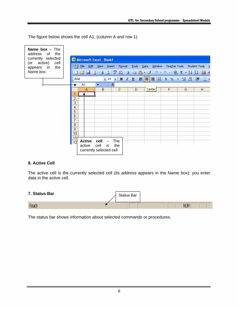
The figure below shows the cell A1, (column A and row 1)
8. Active Cell The active cell is the currently selected cell (its address appears in the Name box); you enter data in the active cell. 7. Status Bar
The status bar shows information about selected commands or procedures.
Name box – The address of the currently selected (or active) cell appears in the Name box.
Active cell – The active cell is the currently selected cell
Status Bar
ICTL for Secondary School programme - Spreadsheet Module
7
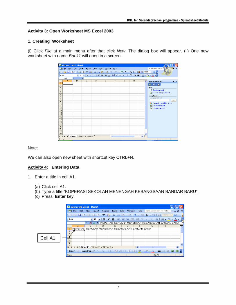
Activity 3: Open Worksheet MS Excel 2003 1. Creating Worksheet (i) Click File at a main menu after that click New. The dialog box will appear. (ii) One new worksheet with name Book1 will open in a screen.
Note:
We can also open new sheet with shortcut key CTRL+N. Activity 4: Entering Data 1. Enter a title in cell A1.
(a) Click cell A1. (b) Type a title “KOPERASI SEKOLAH MENENGAH KEBANGSAAN BANDAR BARU”. (c) Press Enter key.
Cell A1
ICTL for Secondary School programme - Spreadsheet Module
8
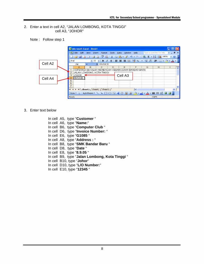
2. Enter a text in cell A2, “JALAN LOMBONG, KOTA TINGGI” cell A3, “JOHOR”
Note : Follow step 1
3. Enter text below
In cell A5, type “Customer “ In cell A6, type “Name:“ In cell B6, type “Computer Club “ In cell D6, type “Invoice Number: “ In cell E6, type “G1085 “ In cell A8, type “Address : “ In cell B8, type “SMK Bandar Baru “ In cell D8, type “Date “ In cell E8, type “8.9.05 “ In cell B9, type “Jalan Lombong, Kota Tinggi “ In cell B10, type “Johor“ In cell D10, type “L/O Number:“ In cell E10, type “12345 “
Cell A2
Cell A4 Cell A3
ICTL for Secondary School programme - Spreadsheet Module
9
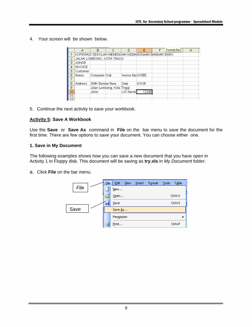
4. Your screen will be shown below.
5. Continue the next activity to save your workbook. Activity 5: Save A Workbook Use the Save or Save As command in File on the bar menu to save the document for the first time. There are few options to save your document. You can choose either one. 1. Save in My Document The following examples shows how you can save a new document that you have open in Activity 1 in Floppy disk. This document will be saving as try.xls in My Document folder. a. Click File on the bar menu.
File
Save
ICTL for Secondary School programme - Spreadsheet Module
10
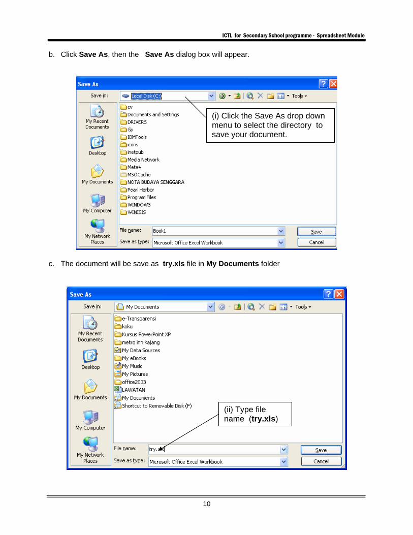
b. Click Save As, then the Save As dialog box will appear.
c. The document will be save as try.xls file in My Documents folder
(i) Click the Save As drop down menu to select the directory to save your document.
(ii) Type file name (try.xls)
ICTL for Secondary School programme - Spreadsheet Module
11
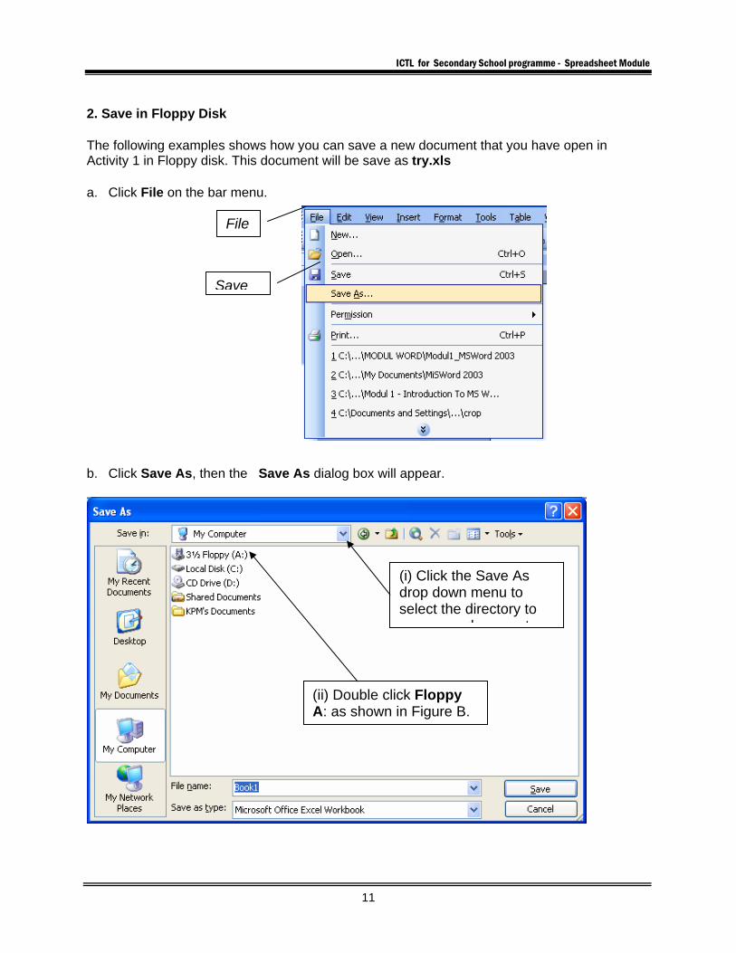
2. Save in Floppy Disk The following examples shows how you can save a new document that you have open in Activity 1 in Floppy disk. This document will be save as try.xls a. Click File on the bar menu. b. Click Save As, then the Save As dialog box will appear.
File
Save
(i) Click the Save As drop down menu to select the directory to
d t
(ii) Double click Floppy A: as shown in Figure B.
ICTL for Secondary School programme - Spreadsheet Module
12
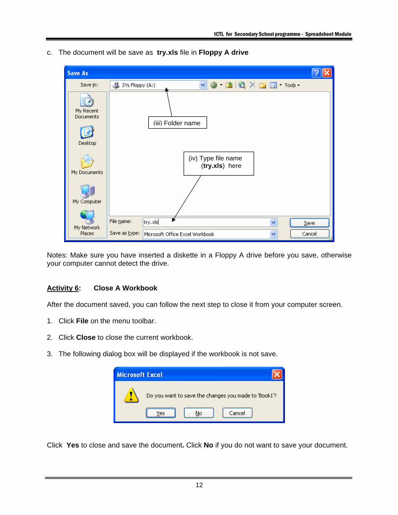
c. The document will be save as try.xls file in Floppy A drive
Notes: Make sure you have inserted a diskette in a Floppy A drive before you save, otherwise your computer cannot detect the drive. Activity 6: Close A Workbook After the document saved, you can follow the next step to close it from your computer screen. 1. Click File on the menu toolbar. 2. Click Close to close the current workbook. 3. The following dialog box will be displayed if the workbook is not save.
Click Yes to close and save the document. Click No if you do not want to save your document.
(iii) Folder name
(iv) Type file name (try.xls) here
ICTL for Secondary School programme - Spreadsheet Module
13
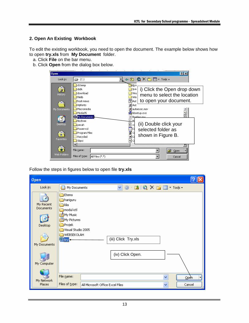
2. Open An Existing Workbook To edit the existing workbook, you need to open the document. The example below shows how to open try.xls from My Document folder.
a. Click File on the bar menu. b. Click Open from the dialog box below.
Follow the steps in figures below to open file try.xls
i) Click the Open drop down menu to select the location to open your document.
(ii) Double click your selected folder as shown in Figure B.
(iii) Click Try.xls
(iv) Click Open.
ICTL for Secondary School programme - Spreadsheet Module
14
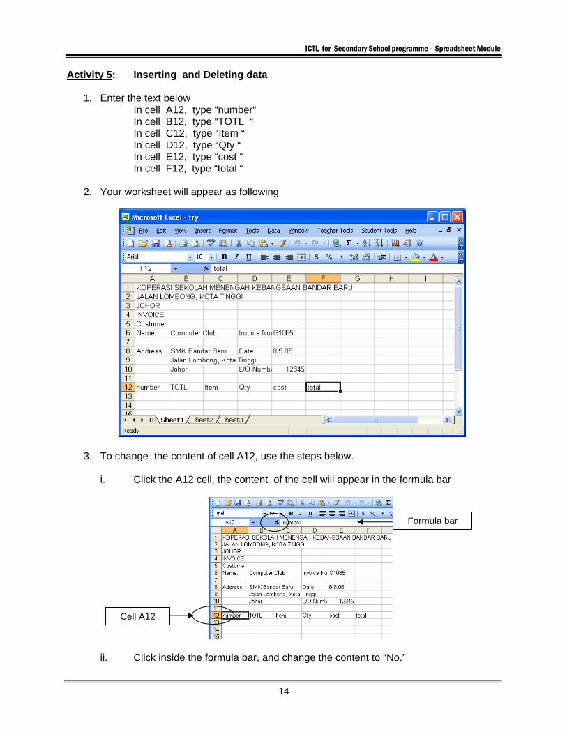
Activity 5: Inserting and Deleting data
1. Enter the text below In cell A12, type “number“ In cell B12, type “TOTL “ In cell C12, type “Item “ In cell D12, type “Qty “ In cell E12, type “cost “ In cell F12, type “total “
2. Your worksheet will appear as following
3. To change the content of cell A12, use the steps below.
i. Click the A12 cell, the content of the cell will appear in the formula bar
ii. Click inside the formula bar, and change the content to “No.”
Cell A12
Formula bar

ICTL for Secondary School programme - Spreadsheet Module
15
4. To edit the content of cell B12, use the steps below.
i. Double Click cell B12, and notice that the cursor will blinking inside the cell instead of on the formula bar.
ii. Edit the cell content, move the cursor before letter “L”, then insert letter “A”.
iii. Click Enter, the new cell content for B12 is “TOTAL” as below.
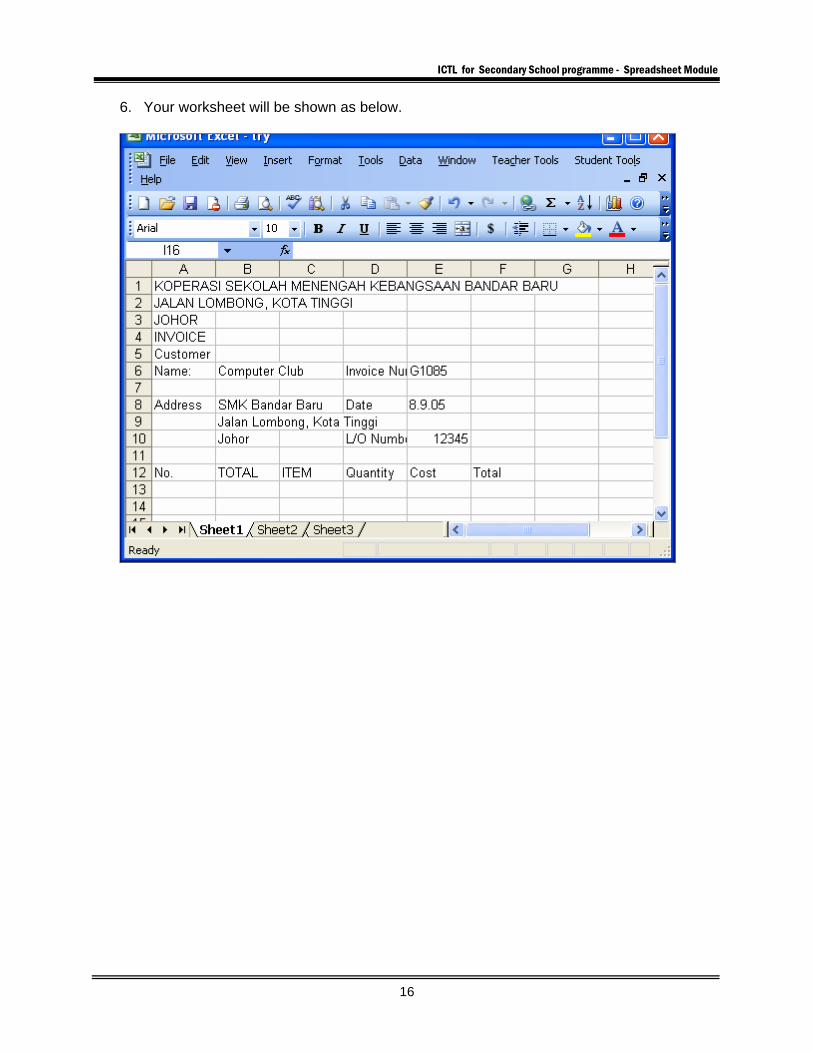
5. Use either step 3 or step 4 to change the following cell content : In cell C12, change “Item “ to “ITEM” In cell D12, change “Qty “ to “Quantity” In cell E12, change “cost “ to “Cost” In cell F12, change “total “ to “Total”
Cell B12
ICTL for Secondary School programme - Spreadsheet Module
16
6. Your worksheet will be shown as below.
ICTL for Secondary School programme - Spreadsheet Module
17
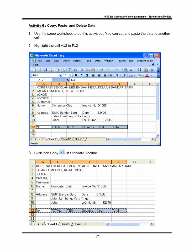
Activity 6 : Copy, Paste and Delete Data 1. Use the same worksheet to do this activities . You can cut and paste the data to another
cell. 2. Highlight the cell A12 to F12
3. Click icon Copy in Standard Toolbar.
ICTL for Secondary School programme - Spreadsheet Module
18
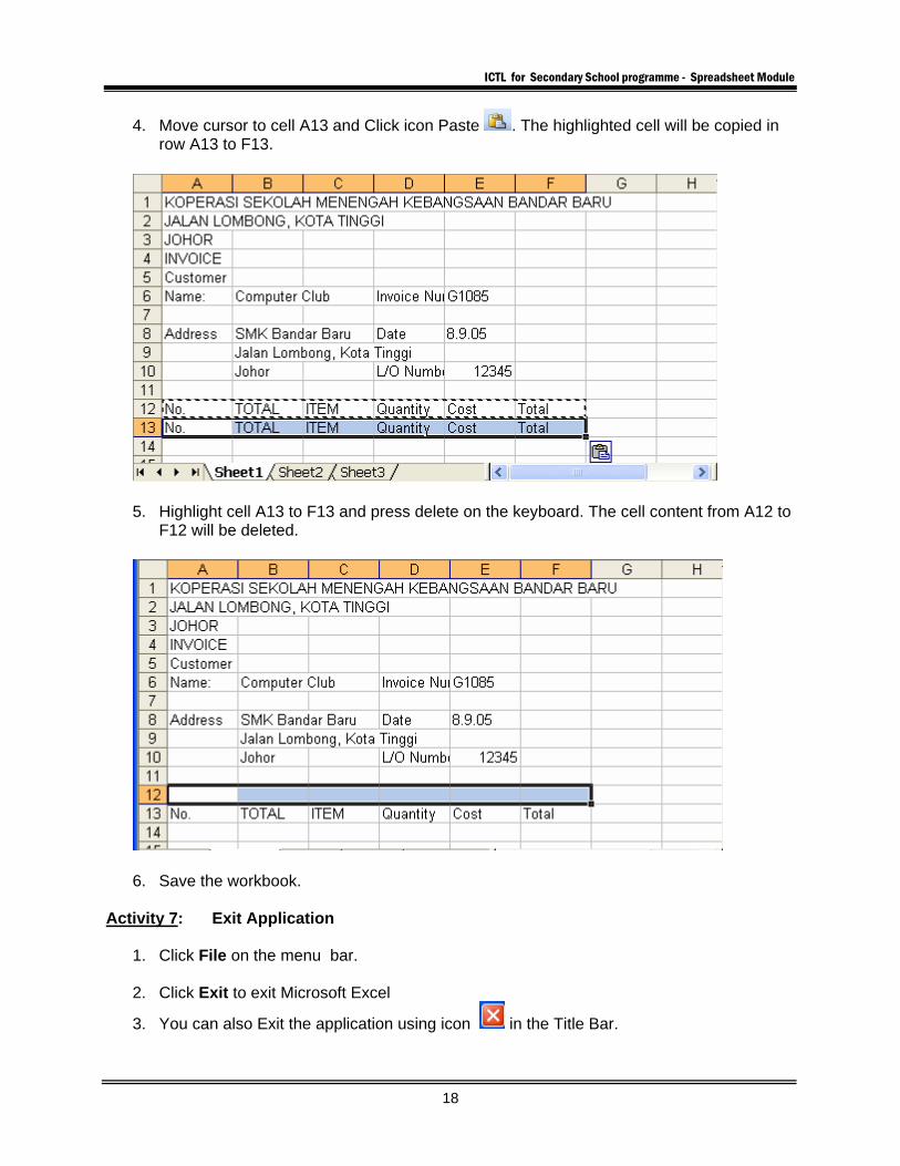
4. Move cursor to cell A13 and Click icon Paste . The highlighted cell will be copied in row A13 to F13.
5. Highlight cell A13 to F13 and press delete on the keyboard. The cell content from A12 to
F12 will be deleted.
6. Save the workbook.
Activity 7: Exit Application
1. Click File on the menu bar.
2. Click Exit to exit Microsoft Excel
3. You can also Exit the application using icon in the Title Bar.
ICTL for Secondary School programme - Spreadsheet Module
19
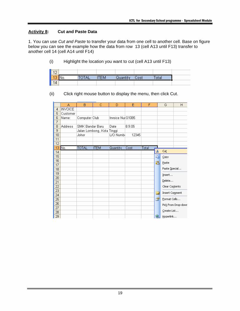
Activity 8: Cut and Paste Data 1. You can use Cut and Paste to transfer your data from one cell to another cell. Base on figure below you can see the example how the data from row 13 (cell A13 until F13) transfer to another cell 14 (cell A14 until F14)
(i) Highlight the location you want to cut (cell A13 until F13)
(ii) Click right mouse button to display the menu, then click Cut.

ICTL for Secondary School programme - Spreadsheet Module
20
(iii) Notice that the selected cells will change to blinking line.
(iv) Place the cursor in Cell A14, Click right mouse button to display the menu,
then click paste. The content of Cells A13 to F13 will be deleted and copied into Cells A14 to F14.
(iii) Save and exit the application.
Notes: Copy and Paste operation is similar with Cut and Paste operation. But the different between the two operations is Copy and Paste operation is not delete the original data. The differences between Cut and Paste with Copy and Paste:
i. Cut and Paste – the highlighted data will be deleted from sentence when Cut was clicked.
ii. Copy and Paste - the highlighted data will not be deleted from sentence when Copy was clicked.
ICTL for Secondary School programme - Spreadsheet Module
21
MODULE 2
INVOICE
Curriculum Development Centre Ministry of Education Malaysia
ICTL for Secondary School programme - Spreadsheet Module
22
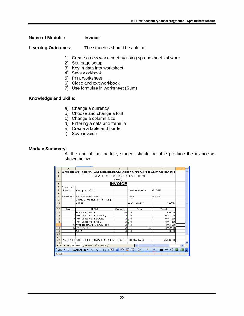
Name of Module : Invoice Learning Outcomes: The students should be able to:
1) Create a new worksheet by using spreadsheet software 2) Set ‘page setup’ 3) Key in data into worksheet 4) Save workbook 5) Print worksheet 6) Close and exit workbook 7) Use formulae in worksheet (Sum)
Knowledge and Skills:
a) Change a currency b) Choose and change a font c) Change a column size d) Entering a data and formula e) Create a table and border f) Save invoice
Module Summary:
At the end of the module, student should be able produce the invoice as shown below.
ICTL for Secondary School programme - Spreadsheet Module
23
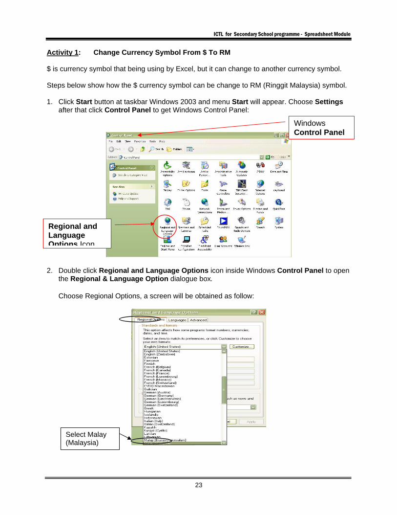
Activity 1: Change Currency Symbol From $ To RM $ is currency symbol that being using by Excel, but it can change to another currency symbol. Steps below show how the $ currency symbol can be change to RM (Ringgit Malaysia) symbol. 1. Click Start button at taskbar Windows 2003 and menu Start will appear. Choose Settings
after that click Control Panel to get Windows Control Panel:
2. Double click Regional and Language Options icon inside Windows Control Panel to open
the Regional & Language Option dialogue box.
Choose Regional Options, a screen will be obtained as follow:
Windows Control Panel
Regional and Language Options Icon
Select Malay (Malaysia)
ICTL for Secondary School programme - Spreadsheet Module
24
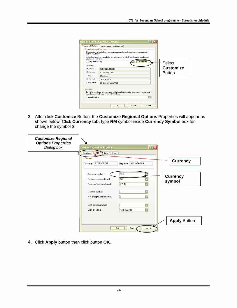
3. After click Customize Button, the Customize Regional Options Properties will appear as shown below. Click Currency tab, type RM symbol inside Currency Symbol box for change the symbol $.
4. Click Apply button then click button OK.
Customize Regional Options Properties
Dialog box
Currency
Currency symbol B
Apply Button
Select Customize Button
ICTL for Secondary School programme - Spreadsheet Module
25
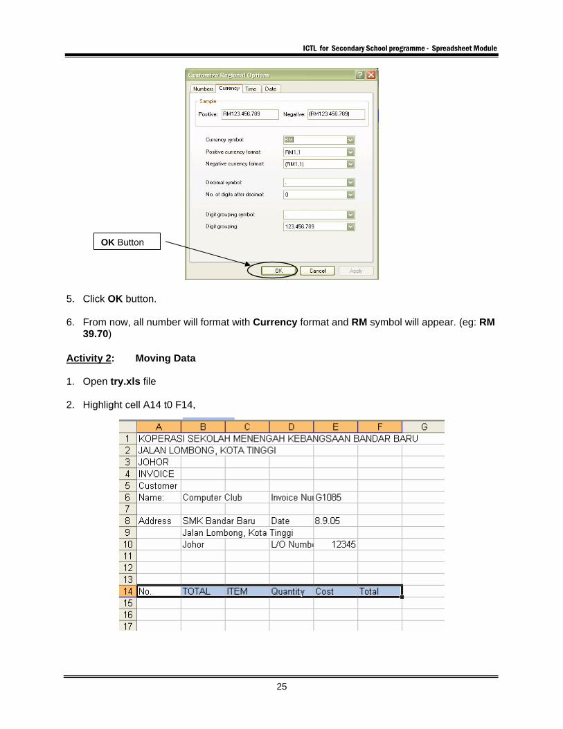
5. Click OK button. 6. From now, all number will format with Currency format and RM symbol will appear. (eg: RM
39.70) Activity 2: Moving Data 1. Open try.xls file 2. Highlight cell A14 t0 F14,
OK Button
ICTL for Secondary School programme - Spreadsheet Module
26
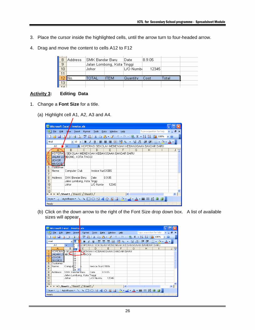
3. Place the cursor inside the highlighted cells, until the arrow turn to four-headed arrow. 4. Drag and move the content to cells A12 to F12
Activity 3: Editing Data 1. Change a Font Size for a title.
(a) Highlight cell A1, A2, A3 and A4.
(b) Click on the down arrow to the right of the Font Size drop down box. A list of available sizes will appear.
ICTL for Secondary School programme - Spreadsheet Module
27
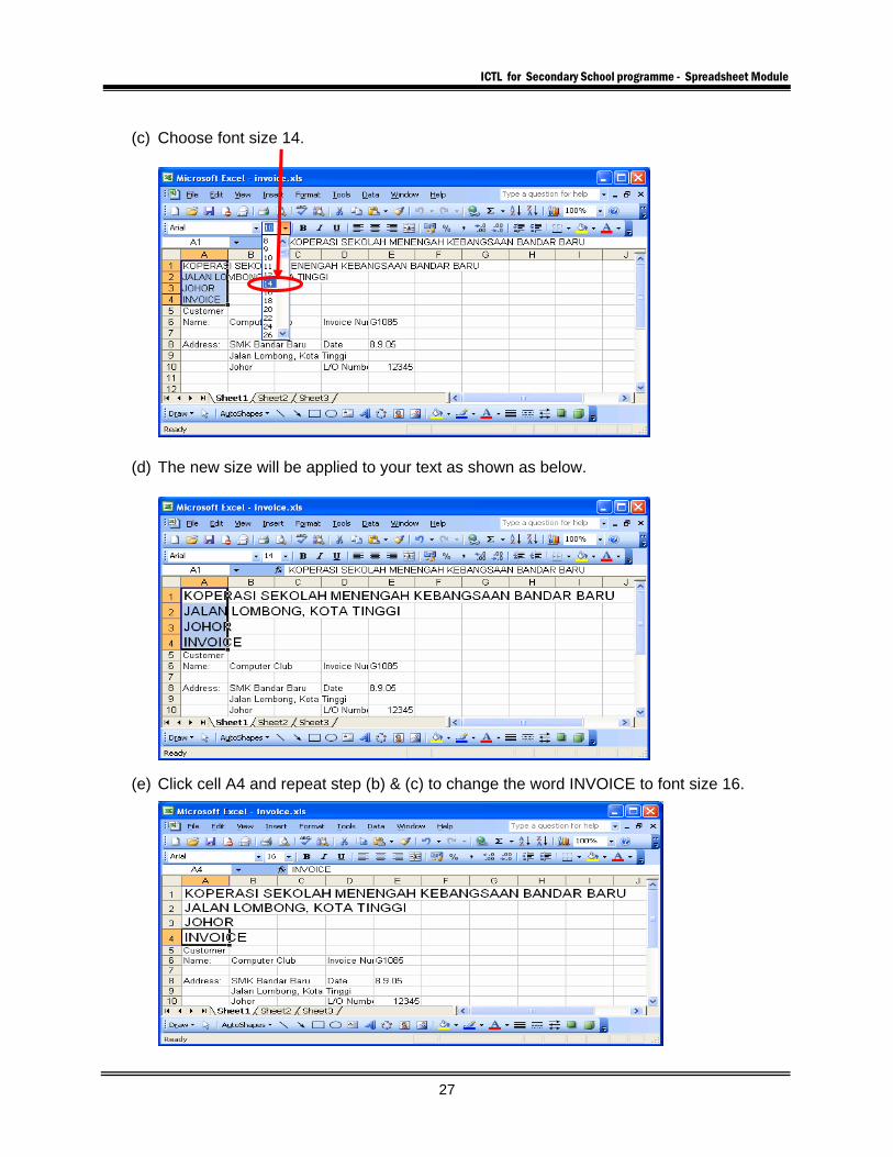
(c) Choose font size 14.
(d) The new size will be applied to your text as shown as below.
(e) Click cell A4 and repeat step (b) & (c) to change the word INVOICE to font size 16.
ICTL for Secondary School programme - Spreadsheet Module
28
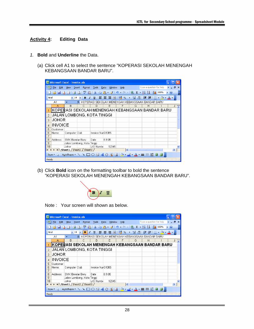
Activity 4: Editing Data 1. Bold and Underline the Data.
(a) Click cell A1 to select the sentence ”KOPERASI SEKOLAH MENENGAH KEBANGSAAN BANDAR BARU”.
(b) Click Bold icon on the formatting toolbar to bold the sentence ”KOPERASI SEKOLAH MENENGAH KEBANGSAAN BANDAR BARU”.
Note : Your screen will shown as below.
ICTL for Secondary School programme - Spreadsheet Module
29
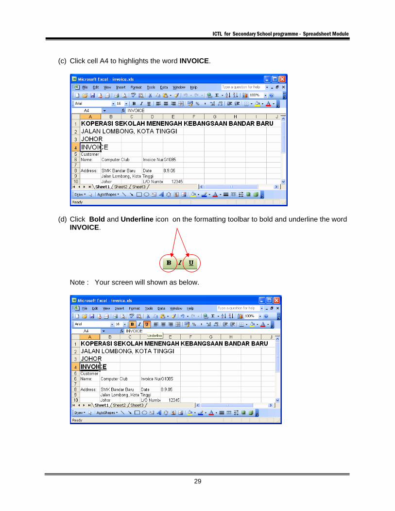
(c) Click cell A4 to highlights the word INVOICE.
(d) Click Bold and Underline icon on the formatting toolbar to bold and underline the word INVOICE.
Note : Your screen will shown as below.
ICTL for Secondary School programme - Spreadsheet Module
30
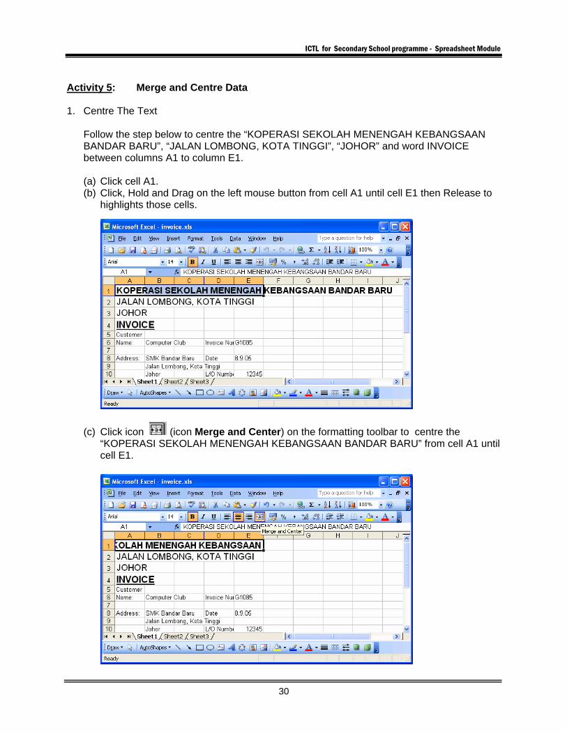
Activity 5: Merge and Centre Data 1. Centre The Text
Follow the step below to centre the “KOPERASI SEKOLAH MENENGAH KEBANGSAAN BANDAR BARU”, “JALAN LOMBONG, KOTA TINGGI”, “JOHOR” and word INVOICE between columns A1 to column E1. (a) Click cell A1. (b) Click, Hold and Drag on the left mouse button from cell A1 until cell E1 then Release to
highlights those cells.
(c) Click icon (icon Merge and Center) on the formatting toolbar to centre the “KOPERASI SEKOLAH MENENGAH KEBANGSAAN BANDAR BARU” from cell A1 until cell E1.
ICTL for Secondary School programme - Spreadsheet Module
31
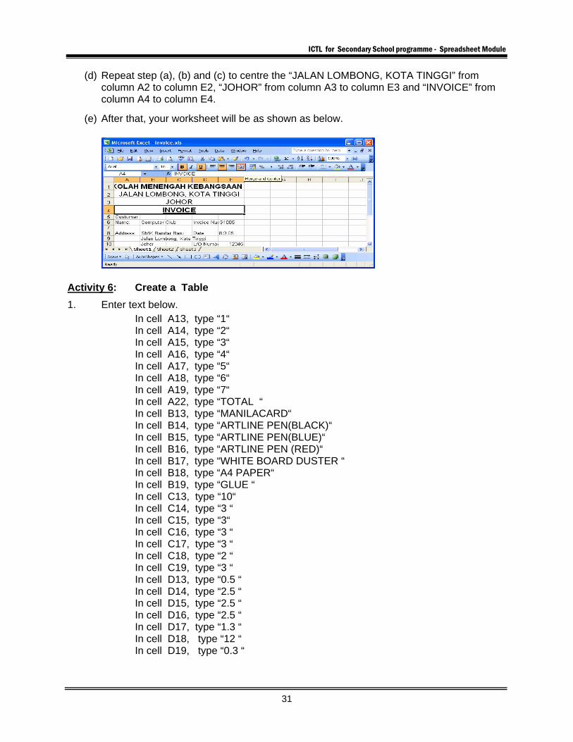
(d) Repeat step (a), (b) and (c) to centre the “JALAN LOMBONG, KOTA TINGGI” from column A2 to column E2, “JOHOR” from column A3 to column E3 and “INVOICE” from column A4 to column E4.
(e) After that, your worksheet will be as shown as below.
Activity 6: Create a Table
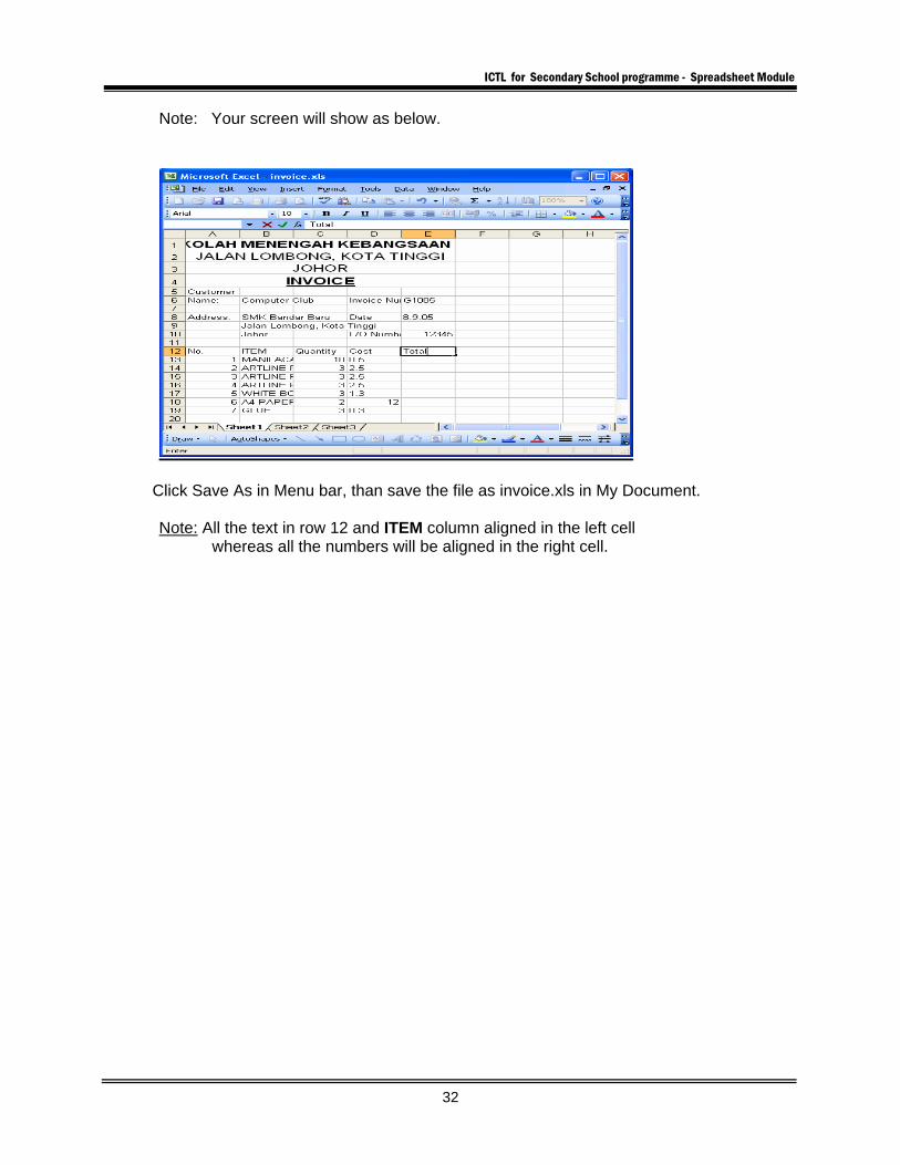
1. Enter text below.
In cell A13, type “1“ In cell A14, type “2“ In cell A15, type “3“ In cell A16, type “4“ In cell A17, type “5“ In cell A18, type “6“ In cell A19, type “7“ In cell A22, type “TOTAL “ In cell B13, type “MANILACARD“ In cell B14, type “ARTLINE PEN(BLACK)“ In cell B15, type “ARTLINE PEN(BLUE)“ In cell B16, type “ARTLINE PEN (RED)“ In cell B17, type “WHITE BOARD DUSTER “ In cell B18, type “A4 PAPER“ In cell B19, type “GLUE “ In cell C13, type “10“ In cell C14, type “3 “ In cell C15, type “3“ In cell C16, type “3 “ In cell C17, type “3 “ In cell C18, type “2 “ In cell C19, type “3 “ In cell D13, type “0.5 “ In cell D14, type “2.5 “ In cell D15, type “2.5 “ In cell D16, type “2.5 “ In cell D17, type “1.3 “ In cell D18, type “12 “ In cell D19, type “0.3 “
ICTL for Secondary School programme - Spreadsheet Module
32
Note: Your screen will show as below.
Click Save As in Menu bar, than save the file as invoice.xls in My Document.
Note: All the text in row 12 and ITEM column aligned in the left cell whereas all the numbers will be aligned in the right cell.
ICTL for Secondary School programme - Spreadsheet Module
33
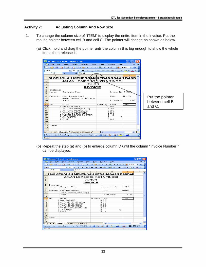
Activity 7: Adjusting Column And Row Size 1. To change the column size of “ITEM” to display the entire item in the invoice. Put the
mouse pointer between cell B and cell C. The pointer will change as shown as below.
(a) Click, hold and drag the pointer until the column B is big enough to show the whole items then release it.
(b) Repeat the step (a) and (b) to enlarge column D until the column “Invoice Number:” can be displayed.
Put the pointer between cell B and C.
ICTL for Secondary School programme - Spreadsheet Module
34
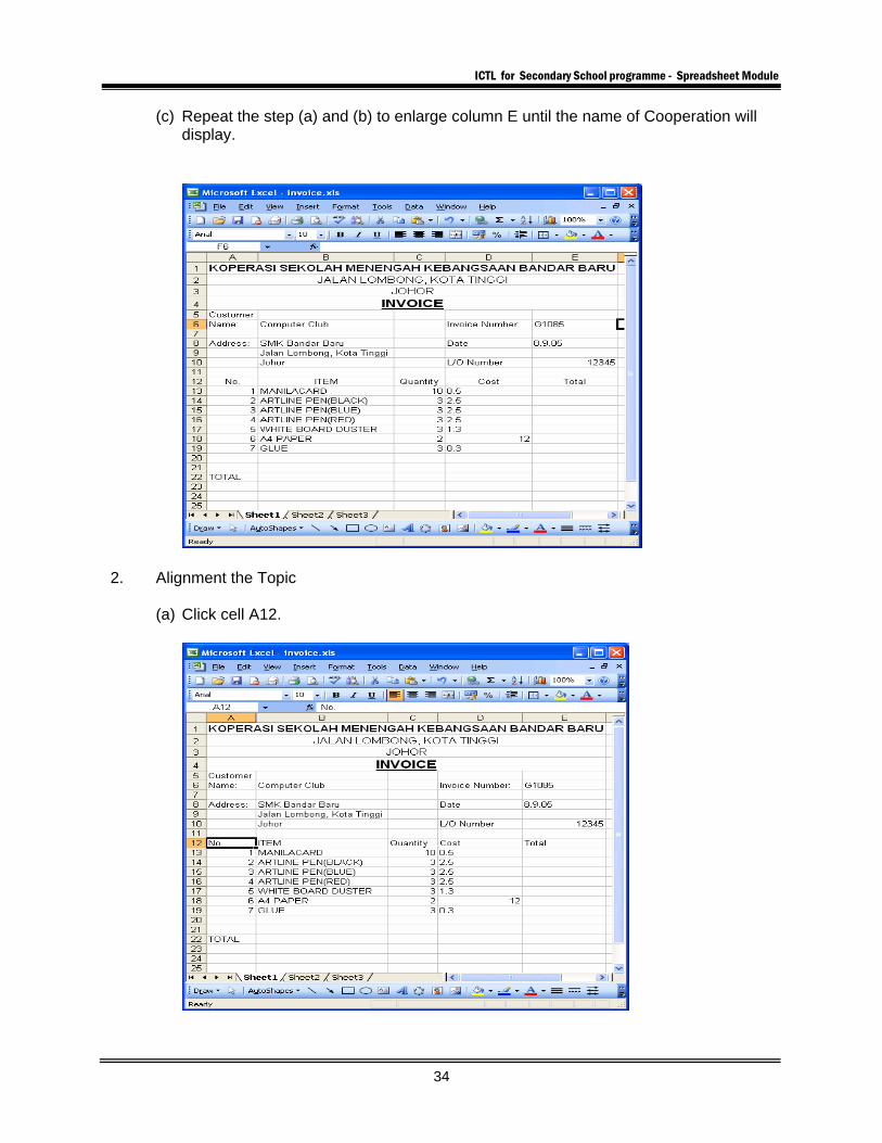
(c) Repeat the step (a) and (b) to enlarge column E until the name of Cooperation will display.
2. Alignment the Topic
(a) Click cell A12.
ICTL for Secondary School programme - Spreadsheet Module
35
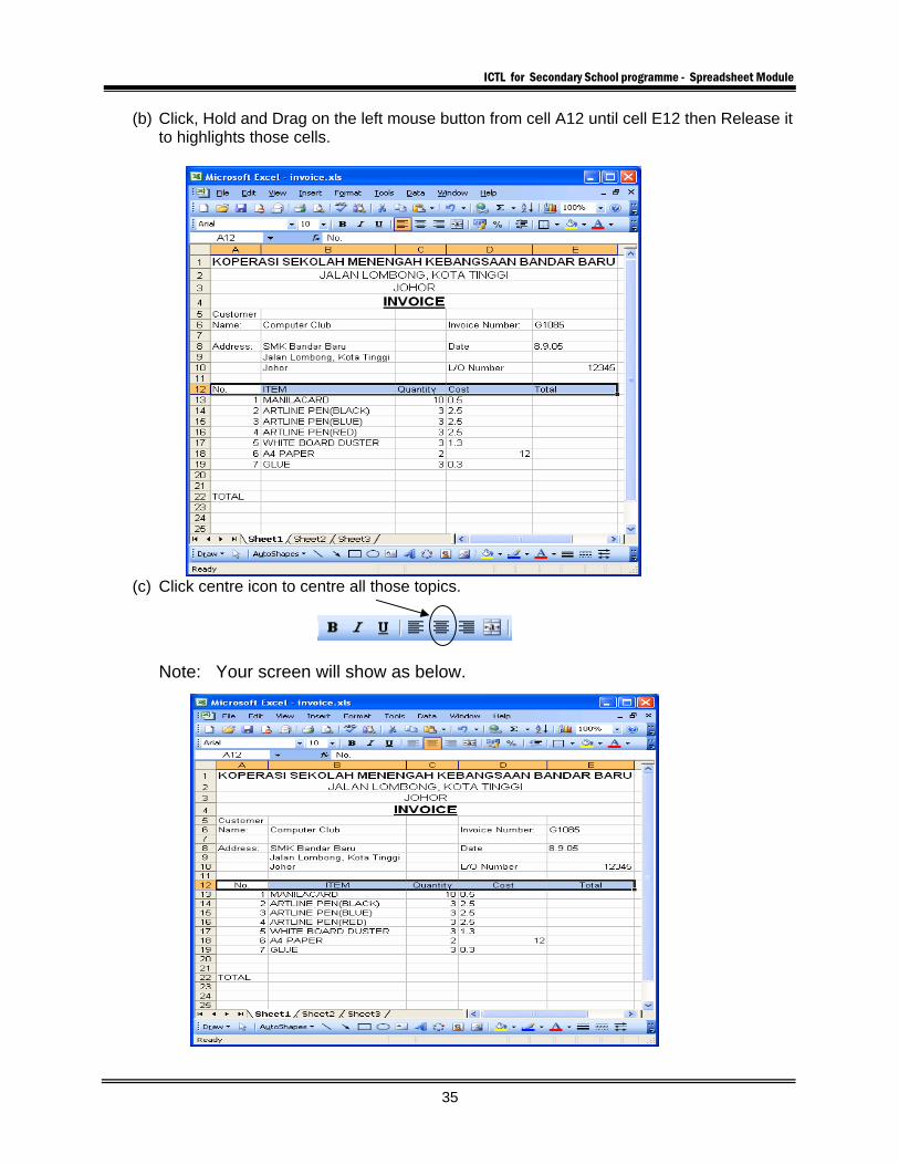
(b) Click, Hold and Drag on the left mouse button from cell A12 until cell E12 then Release it to highlights those cells.
(c) Click centre icon to centre all those topics.
Note: Your screen will show as below.
ICTL for Secondary School programme - Spreadsheet Module
36
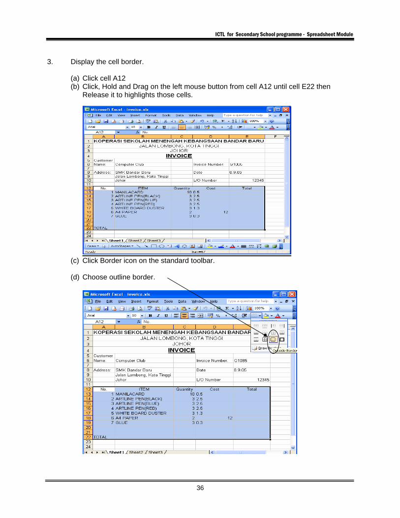
3. Display the cell border.
(a) Click cell A12 (b) Click, Hold and Drag on the left mouse button from cell A12 until cell E22 then
Release it to highlights those cells.
(c) Click Border icon on the standard toolbar. (d) Choose outline border.
ICTL for Secondary School programme - Spreadsheet Module
37
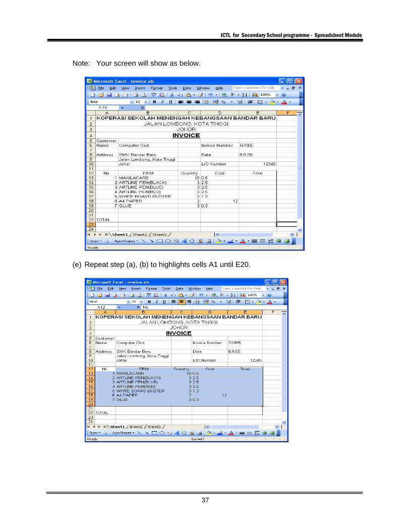
Note: Your screen will show as below.
(e) Repeat step (a), (b) to highlights cells A1 until E20.
ICTL for Secondary School programme - Spreadsheet Module
38
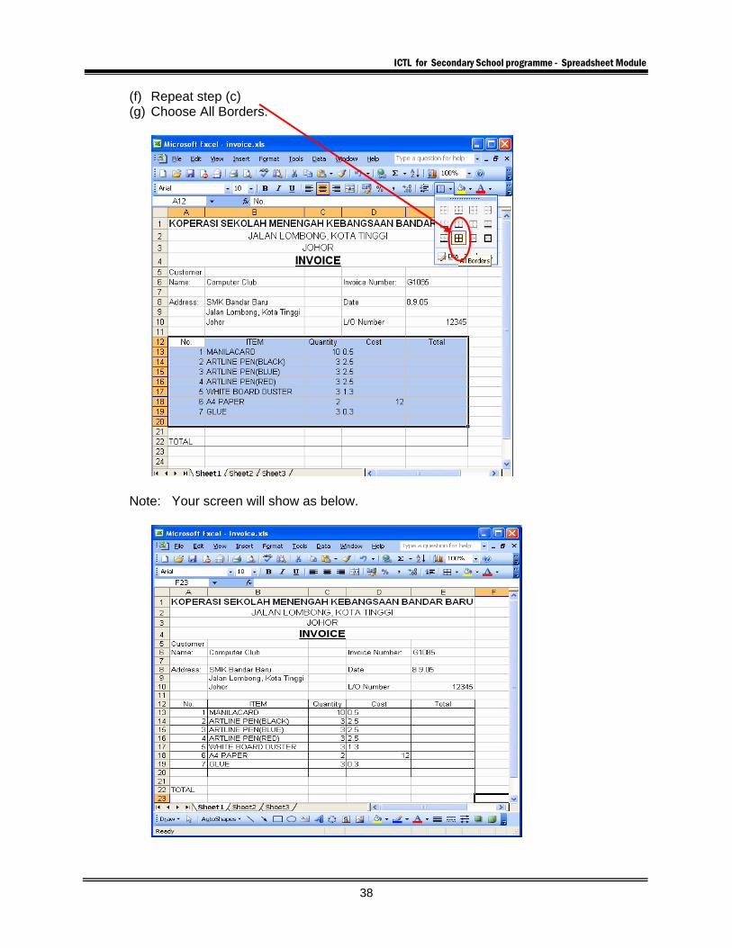
(f) Repeat step (c) (g) Choose All Borders.
Note: Your screen will show as below.
ICTL for Secondary School programme - Spreadsheet Module
39
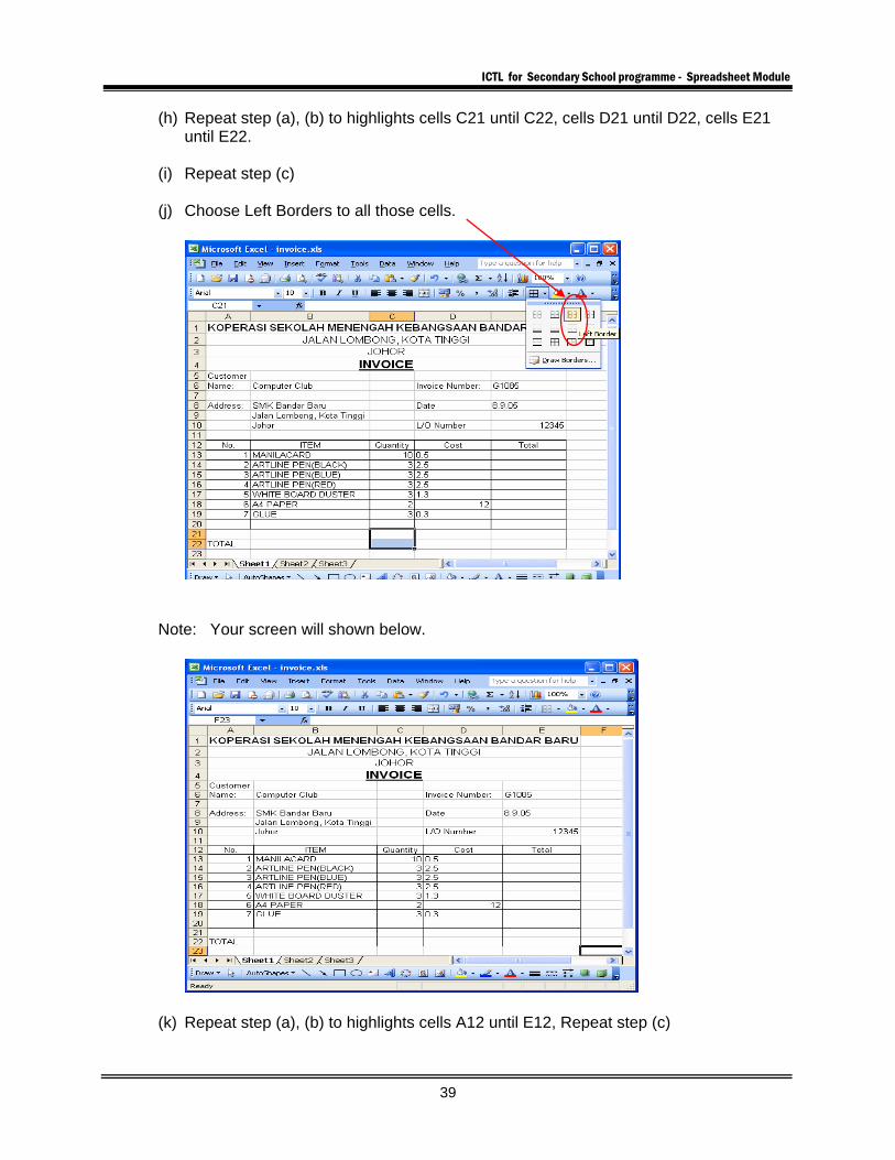
(h) Repeat step (a), (b) to highlights cells C21 until C22, cells D21 until D22, cells E21 until E22.
(i) Repeat step (c)
(j) Choose Left Borders to all those cells.
Note: Your screen will shown below.
(k) Repeat step (a), (b) to highlights cells A12 until E12, Repeat step (c)
ICTL for Secondary School programme - Spreadsheet Module
40
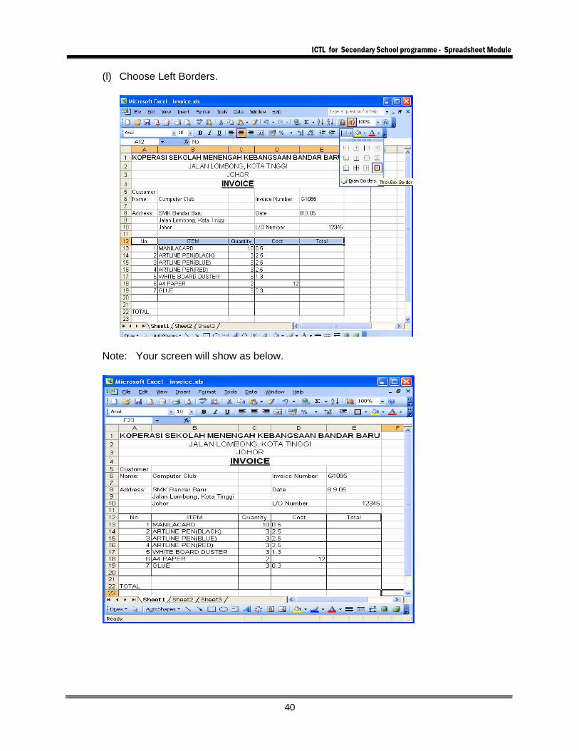
(l) Choose Left Borders.
Note: Your screen will show as below.
ICTL for Secondary School programme - Spreadsheet Module
41
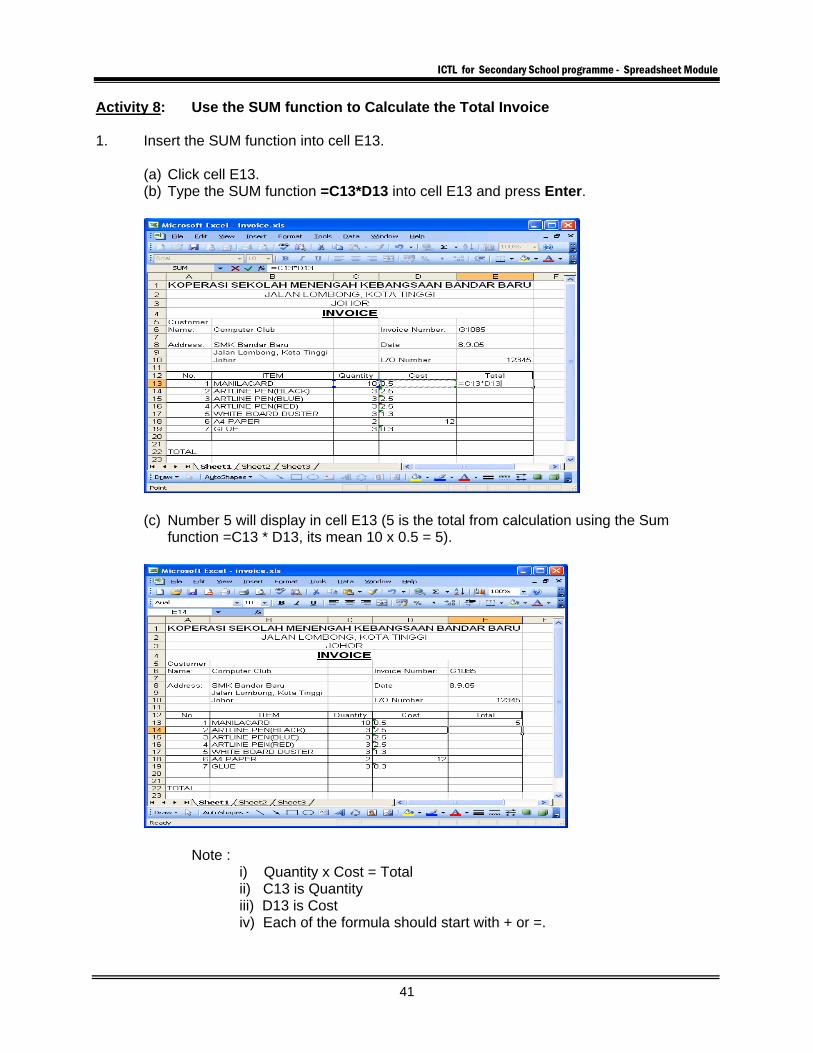
Activity 8: Use the SUM function to Calculate the Total Invoice 1. Insert the SUM function into cell E13.
(a) Click cell E13. (b) Type the SUM function =C13*D13 into cell E13 and press Enter.
(c) Number 5 will display in cell E13 (5 is the total from calculation using the Sum function =C13 * D13, its mean 10 x 0.5 = 5).
Note : i) Quantity x Cost = Total ii) C13 is Quantity iii) D13 is Cost iv) Each of the formula should start with + or =.
ICTL for Secondary School programme - Spreadsheet Module
42
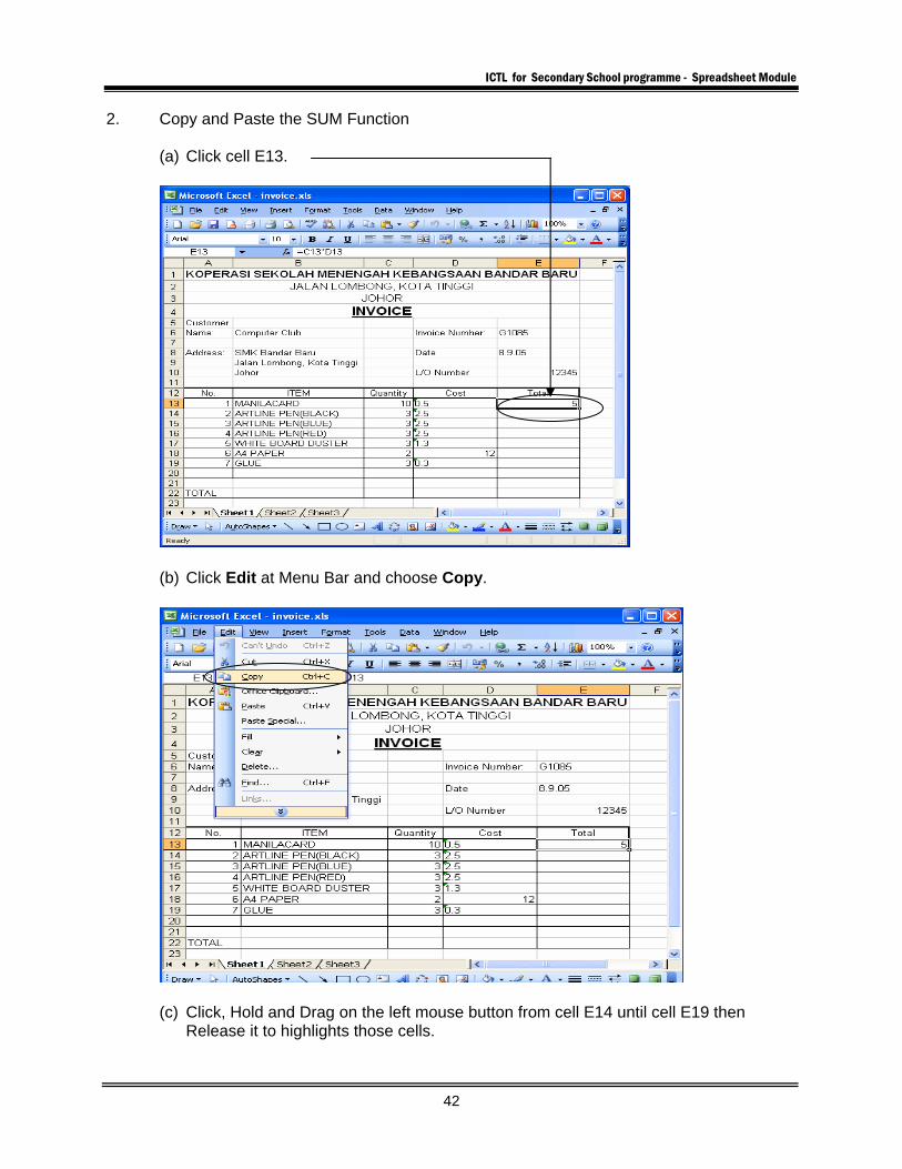
2. Copy and Paste the SUM Function
(a) Click cell E13.
(b) Click Edit at Menu Bar and choose Copy.
(c) Click, Hold and Drag on the left mouse button from cell E14 until cell E19 then Release it to highlights those cells.
ICTL for Secondary School programme - Spreadsheet Module
43
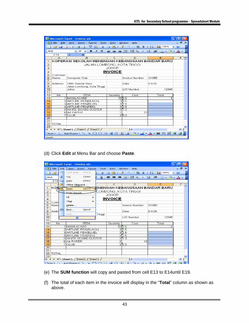
(d) Click Edit at Menu Bar and choose Paste.
(e) The SUM function will copy and pasted from cell E13 to E14until E19. (f) The total of each item in the invoice will display in the “Total” column as shown as
above.
ICTL for Secondary School programme - Spreadsheet Module
44
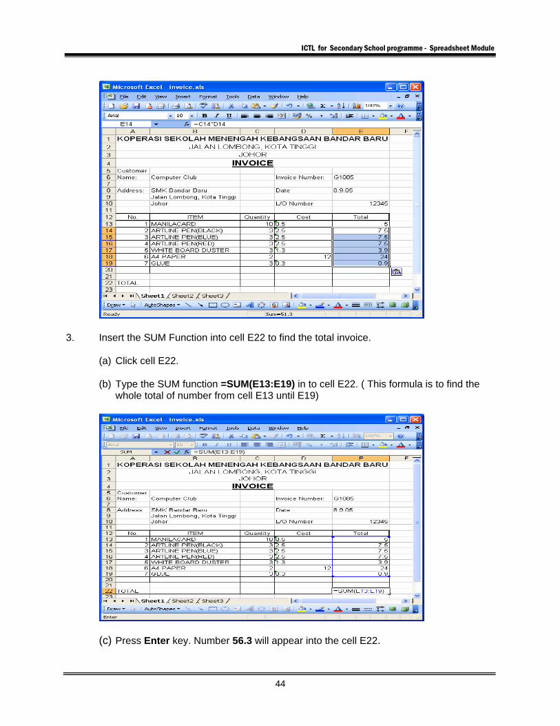
3. Insert the SUM Function into cell E22 to find the total invoice.
(a) Click cell E22. (b) Type the SUM function =SUM(E13:E19) in to cell E22. ( This formula is to find the
whole total of number from cell E13 until E19)
(c) Press Enter key. Number 56.3 will appear into the cell E22.

ICTL for Secondary School programme - Spreadsheet Module
45
(d) Click cell A22 and type text “RINGGIT LIMA PULUH ENAM DAN SEN TIGA
PULUH SAHAJA” into the cell A22.
ICTL for Secondary School programme - Spreadsheet Module
46
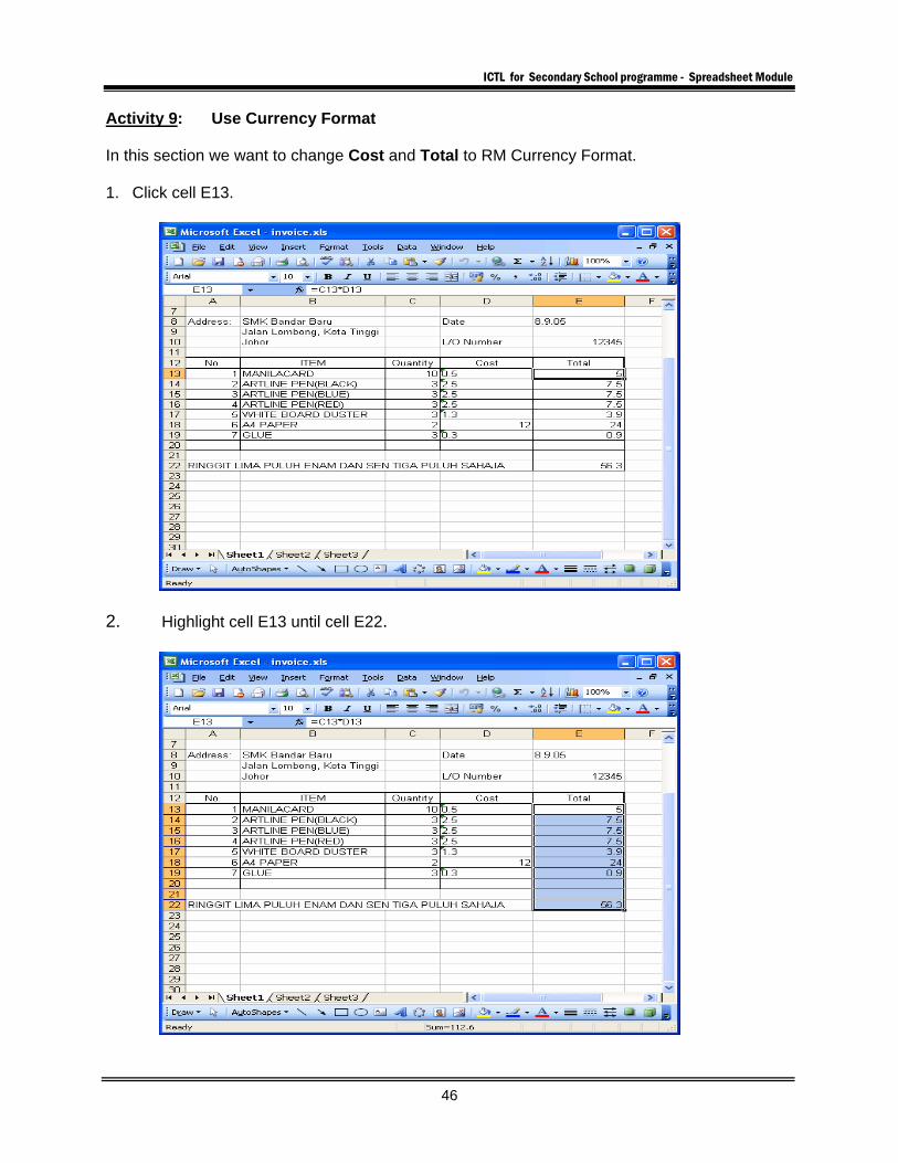
Activity 9: Use Currency Format In this section we want to change Cost and Total to RM Currency Format. 1. Click cell E13.
2. Highlight cell E13 until cell E22.
ICTL for Secondary School programme - Spreadsheet Module
47
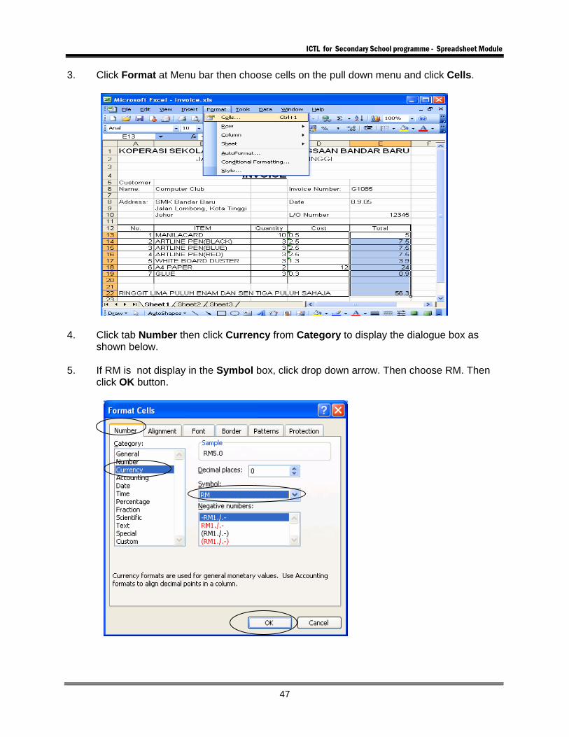
3. Click Format at Menu bar then choose cells on the pull down menu and click Cells.
4. Click tab Number then click Currency from Category to display the dialogue box as
shown below. 5. If RM is not display in the Symbol box, click drop down arrow. Then choose RM. Then
click OK button.
ICTL for Secondary School programme - Spreadsheet Module
48
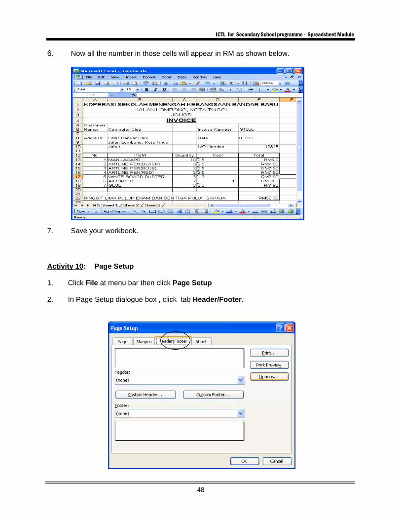
6. Now all the number in those cells will appear in RM as shown below.
7. Save your workbook. Activity 10: Page Setup 1. Click File at menu bar then click Page Setup 2. In Page Setup dialogue box , click tab Header/Footer.
ICTL for Secondary School programme - Spreadsheet Module
49
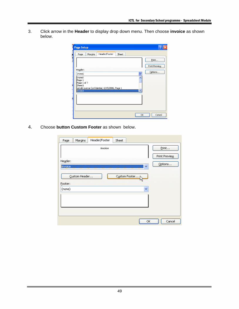
3. Click arrow in the Header to display drop down menu. Then choose invoice as shown below.
4. Choose button Custom Footer as shown below.
ICTL for Secondary School programme - Spreadsheet Module
50
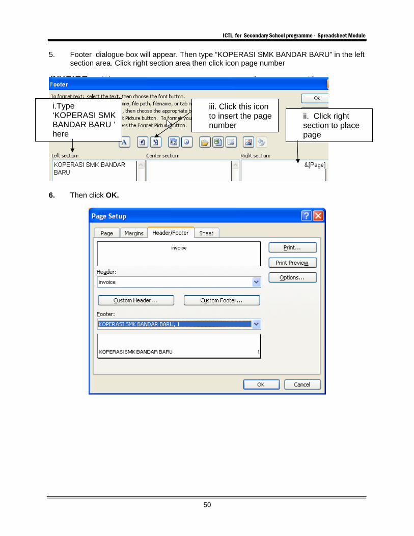
5. Footer dialogue box will appear. Then type “KOPERASI SMK BANDAR BARU” in the left section area. Click right section area then click icon page number
6. Then click OK.
iii. Click this icon to insert the page number
i.Type ‘KOPERASI SMK BANDAR BARU ’ here
ii. Click right section to place page
ICTL for Secondary School programme - Spreadsheet Module
51
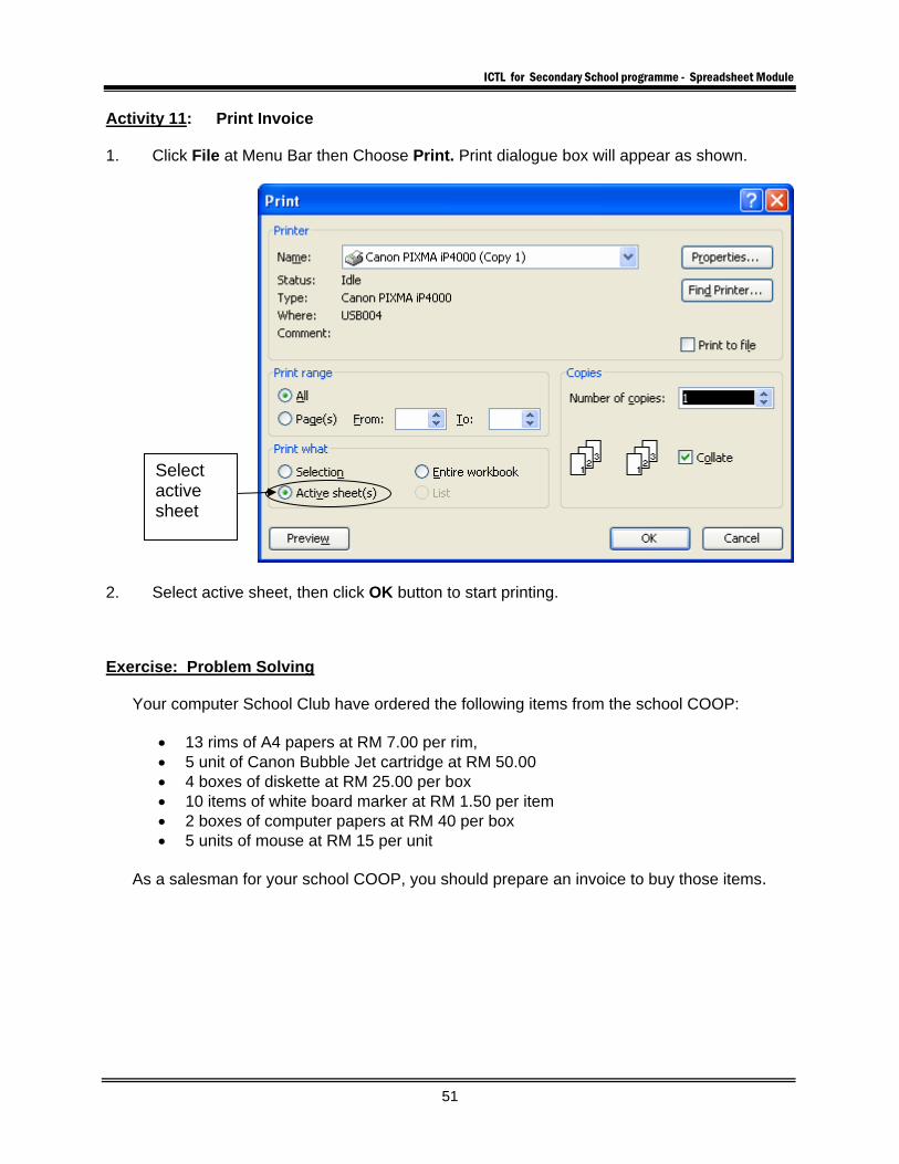
Activity 11: Print Invoice 1. Click File at Menu Bar then Choose Print. Print dialogue box will appear as shown.
2. Select active sheet, then click OK button to start printing. Exercise: Problem Solving
Your computer School Club have ordered the following items from the school COOP:
• 13 rims of A4 papers at RM 7.00 per rim, • 5 unit of Canon Bubble Jet cartridge at RM 50.00 • 4 boxes of diskette at RM 25.00 per box • 10 items of white board marker at RM 1.50 per item • 2 boxes of computer papers at RM 40 per box • 5 units of mouse at RM 15 per unit
As a salesman for your school COOP, you should prepare an invoice to buy those items.
Select active sheet
ICTL for Secondary School programme - Spreadsheet Module
52
MODULE 3
UNIT CHANGE
Curriculum Development Centre Ministry of Education Malaysia
ICTL for Secondary School programme - Spreadsheet Module
53
Name of Module : Unit Change Learning Outcomes: The students should be able to:
1) Using currency format 2) Key in data into worksheet 3) Inserting table 4) Save workbook 5) Close and exit workbook 6) Use formulae in worksheet
Knowledge and Skills:
a) Entering text b) Change the font typeface, font style, and font size c) Text Alignment d) Formatting Cell e) Entering formula f) Using unit change spreadsheet g) Printing spreadsheet
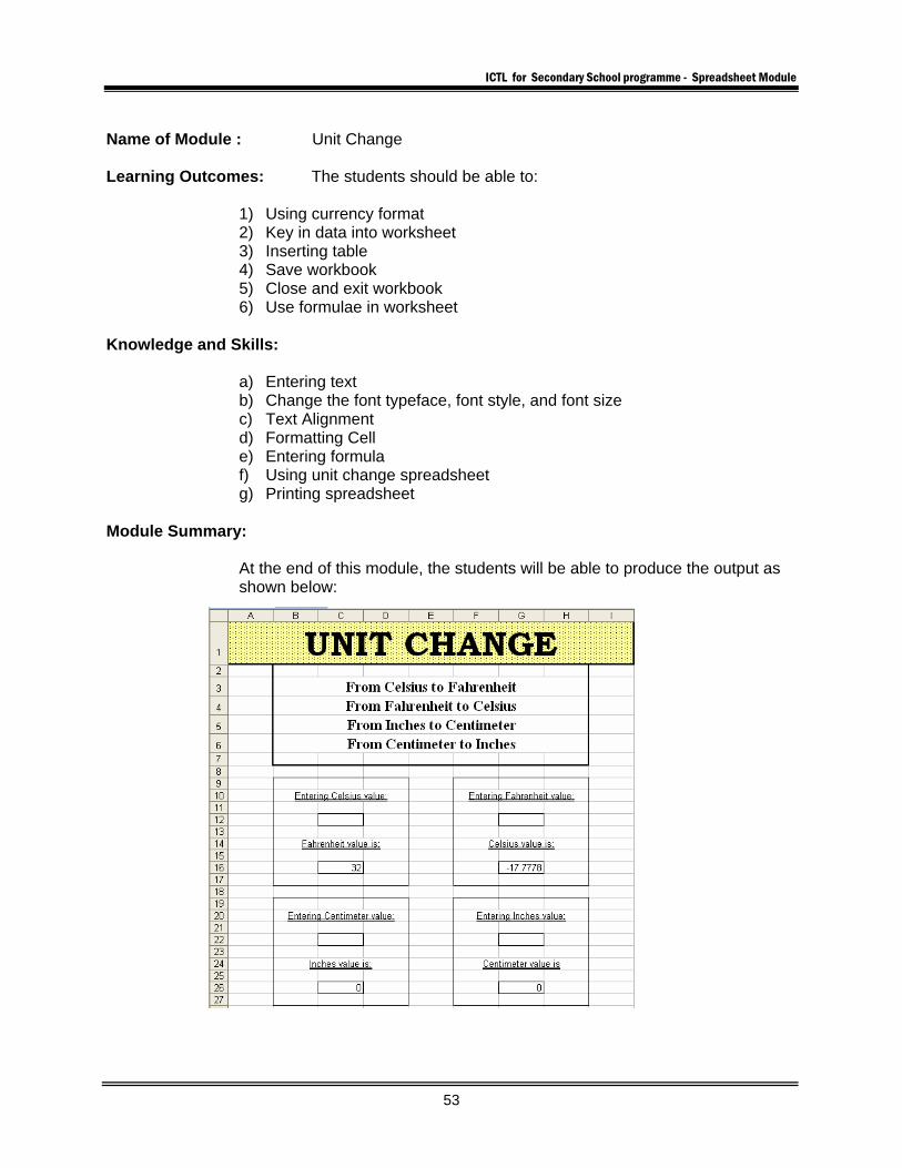
Module Summary:
At the end of this module, the students will be able to produce the output as shown below:
ICTL for Secondary School programme - Spreadsheet Module
54
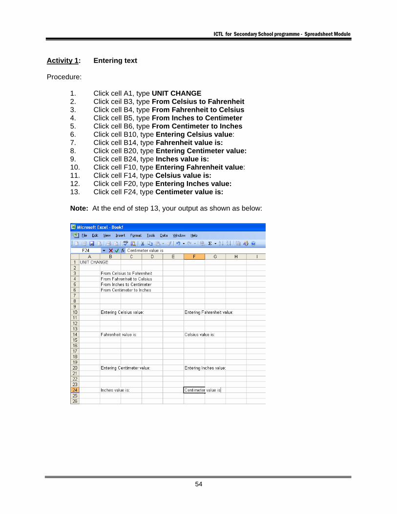
Activity 1: Entering text Procedure:
1. Click cell A1, type UNIT CHANGE 2. Click ceil B3, type From Celsius to Fahrenheit 3. Click cell B4, type From Fahrenheit to Celsius 4. Click cell B5, type From Inches to Centimeter 5. Click cell B6, type From Centimeter to Inches 6. Click cell B10, type Entering Celsius value: 7. Click cell B14, type Fahrenheit value is: 8. Click cell B20, type Entering Centimeter value: 9. Click cell B24, type Inches value is: 10. Click cell F10, type Entering Fahrenheit value: 11. Click cell F14, type Celsius value is: 12. Click cell F20, type Entering Inches value: 13. Click cell F24, type Centimeter value is: Note: At the end of step 13, your output as shown as below:
ICTL for Secondary School programme - Spreadsheet Module
55
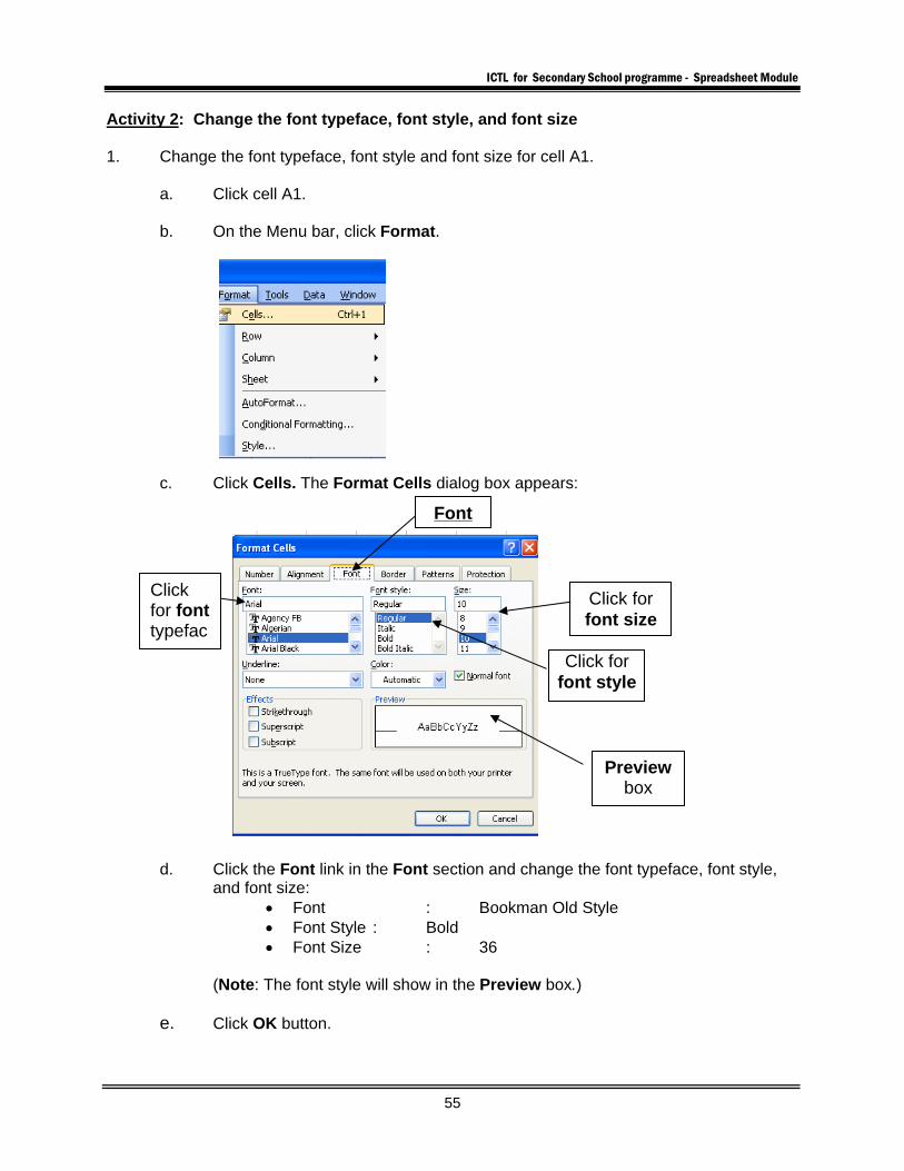
Activity 2: Change the font typeface, font style, and font size 1. Change the font typeface, font style and font size for cell A1.
a. Click cell A1. b. On the Menu bar, click Format.
c. Click Cells. The Format Cells dialog box appears:
d. Click the Font link in the Font section and change the font typeface, font style, and font size:
• Font : Bookman Old Style • Font Style : Bold • Font Size : 36
(Note: The font style will show in the Preview box.)
e. Click OK button.
Font
Click for font size
Click for font style
Click for font typefac
Preview box
ICTL for Secondary School programme - Spreadsheet Module
56
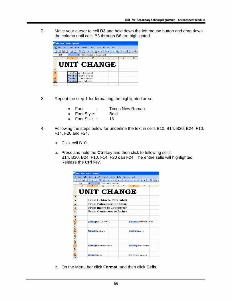
2. Move your cursor to cell B3 and hold down the left mouse button and drag down the column until cells B3 through B6 are highlighted.
3. Repeat the step 1 for formatting the highlighted area:
• Font : Times New Roman • Font Style: Bold • Font Size : 16
4. Following the steps below for underline the text in cells B10, B14, B20, B24, F10,
F14, F20 and F24.
a. Click cell B10. b. Press and hold the Ctrl key and then click to following sells:
B14, B20, B24, F10, F14, F20 dan F24. The entire sells will highlighted. Release the Ctrl key.
c. On the Menu bar click Format, and then click Cells.
ICTL for Secondary School programme - Spreadsheet Module
57
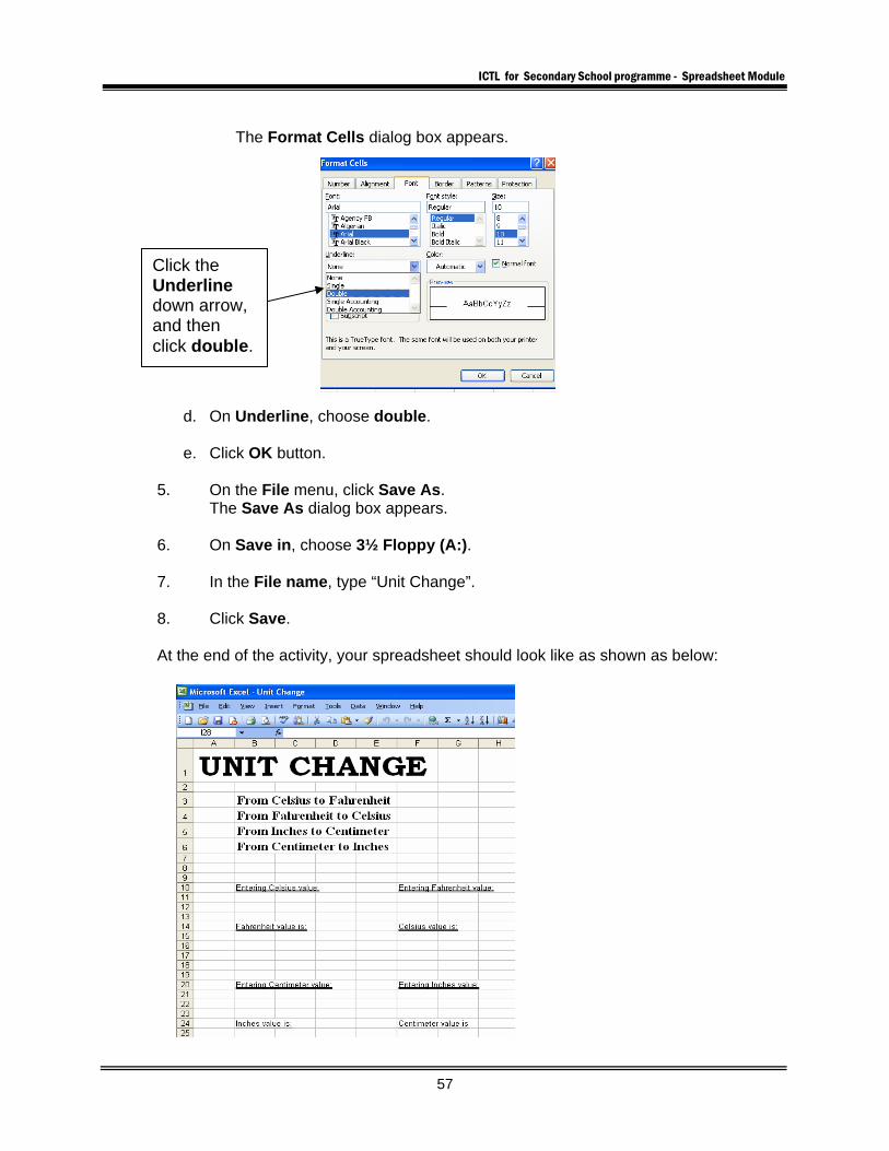
The Format Cells dialog box appears.
d. On Underline, choose double. e. Click OK button.
5. On the File menu, click Save As. The Save As dialog box appears. 6. On Save in, choose 3½ Floppy (A:). 7. In the File name, type “Unit Change”. 8. Click Save.
At the end of the activity, your spreadsheet should look like as shown as below:
Click the Underline down arrow, and then click double.
ICTL for Secondary School programme - Spreadsheet Module
58
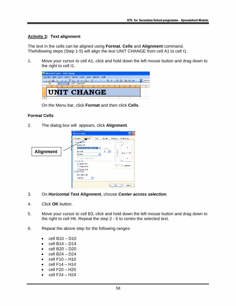
Activity 3: Text alignment The text in the cells can be aligned using Format, Cells and Alignment command. Thefollowing steps (Step 1-5) will align the text UNIT CHANGE from cell A1 to cell I1.
1. Move your cursor to cell A1, click and hold down the left mouse button and drag down to
the right to cell I1.
On the Menu bar, click Format and then click Cells. Format Cells 2. The dialog box will appears, click Alignment. 3. On Horizontal Text Alignment, choose Center across selection. 4. Click OK button. 5. Move your cursor to cell B3, click and hold down the left mouse button and drag down to
the right to cell H6. Repeat the step 2 - 5 to centre the selected text. 6. Repeat the above step for the following ranges:
• cell B10 – D10 • cell B14 – D14 • cell B20 – D20 • cell B24 – D24 • cell F10 – H10 • cell F14 – H14 • cell F20 – H20 • cell F24 – H24
Alignment

ICTL for Secondary School programme - Spreadsheet Module
59
Note: At the end of the activity, your spreadsheet should look like as shown as below:
ICTL for Secondary School programme - Spreadsheet Module
60
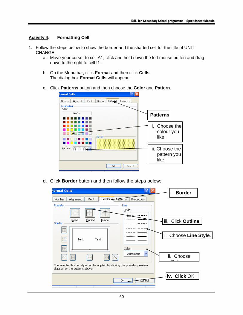
Activity 4: Formatting Cell
1. Follow the steps below to show the border and the shaded cell for the title of UNIT
CHANGE. a. Move your cursor to cell A1, click and hold down the left mouse button and drag
down to the right to cell I1. b. On the Menu bar, click Format and then click Cells.
The dialog box Format Cells will appear.
c. Click Patterns button and then choose the Color and Pattern. d. Click Border button and then follow the steps below:
ii. Choose the pattern you like.
i. Choose the colour you like.
Patterns
Border
iv. Click OK
ii. Choose Colo r
iii. Click Outline.
i. Choose Line Style.
ICTL for Secondary School programme - Spreadsheet Module
61
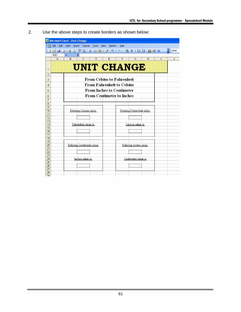
2. Use the above steps to create borders as shown below:
ICTL for Secondary School programme - Spreadsheet Module
62
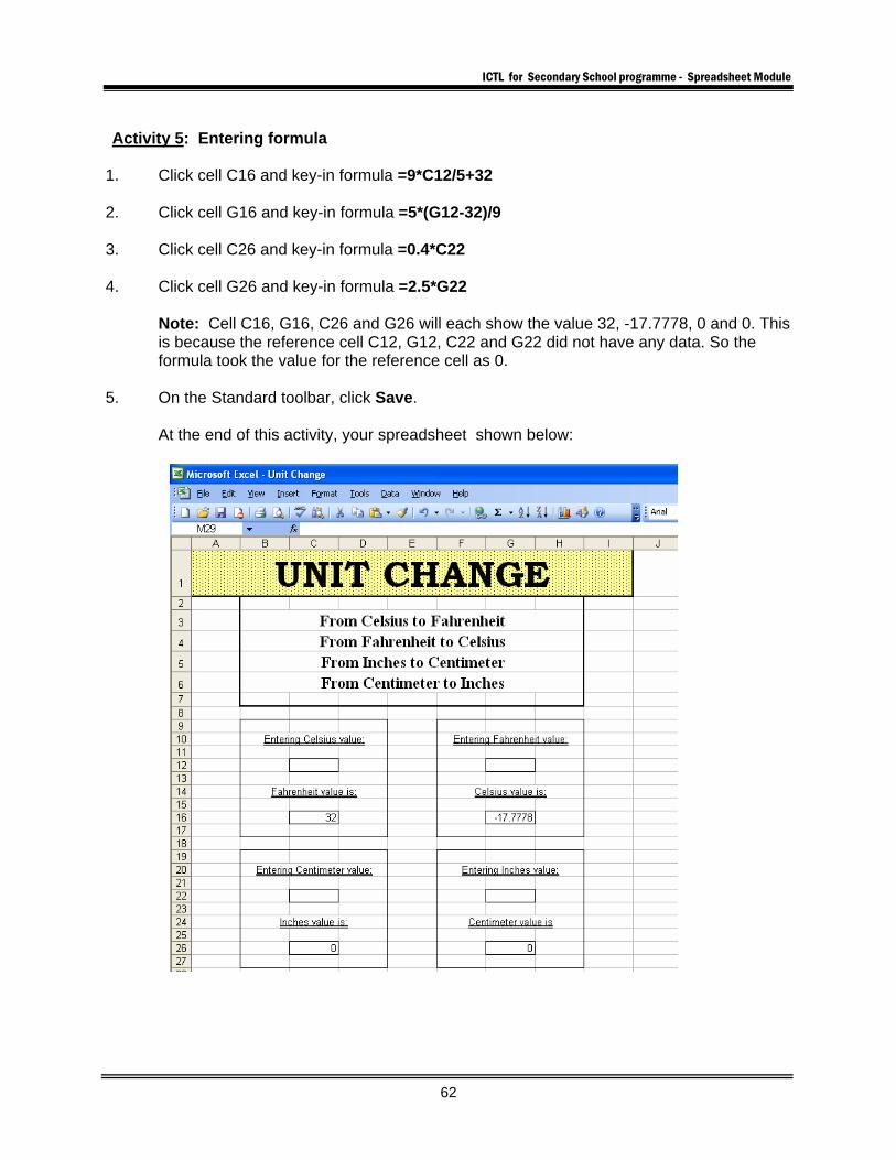
Activity 5: Entering formula
1. Click cell C16 and key-in formula =9*C12/5+32 2. Click cell G16 and key-in formula =5*(G12-32)/9 3. Click cell C26 and key-in formula =0.4*C22 4. Click cell G26 and key-in formula =2.5*G22
Note: Cell C16, G16, C26 and G26 will each show the value 32, -17.7778, 0 and 0. This is because the reference cell C12, G12, C22 and G22 did not have any data. So the formula took the value for the reference cell as 0.
5. On the Standard toolbar, click Save. At the end of this activity, your spreadsheet shown below:
ICTL for Secondary School programme - Spreadsheet Module
63
Activity 6: Using unit change spreadsheet
1. To change the Celsius unit to Fahrenheit unit: • Click cell C12. • Entering a temperature value into that cell. • The Fahrenheit unit for that temperature will appears on the cell C16.
2. To change the Fahrenheit unit to Celsius unit:
• Click cell G12. • Entering a temperature value into that cell. • The Celsius unit for that temperature will appears on the cell G16.
3. To change the centimeter unit to inches unit:
• Click cell C22. • Entering a value into that cell. • The inches unit for that value will appears on the cell C26.
4. To change the inches unit to centimeter unit:
• Click cell G22. • Entering a value into that cell. • The Centimeter unit for that value will appears on the cell G26.
ICTL for Secondary School programme - Spreadsheet Module
64
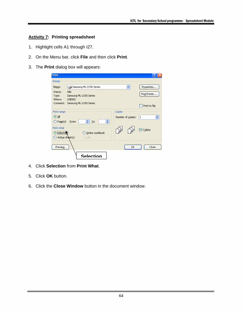
Activity 7: Printing spreadsheet
1. Highlight cells A1 through I27. 2. On the Menu bar, click File and then click Print. 3. The Print dialog box will appears: 4. Click Selection from Print What. 5. Click OK button. 6. Click the Close Window button in the document window.
Selection
ICTL for Secondary School programme - Spreadsheet Module
65
MODULE 4
MARKSHEET
Curriculum Development Centre Ministry of Education Malaysia
ICTL for Secondary School programme - Spreadsheet Module
66
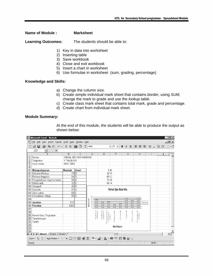
Name of Module : Marksheet Learning Outcomes: The students should be able to:
1) Key in data into worksheet 2) Inserting table 3) Save workbook 4) Close and exit workbook 5) Insert a chart in worksheet 6) Use formulae in worksheet (sum, grading, percentage)
Knowledge and Skills:
a) Change the column size. b) Create simple individual mark sheet that contains border, using SUM,
change the mark to grade and use the lookup table. c) Create class mark sheet that contains total mark, grade and percentage. d) Create chart from individual mark sheet.
Module Summary:
At the end of this module, the students will be able to produce the output as shown below:
ICTL for Secondary School programme - Spreadsheet Module
67
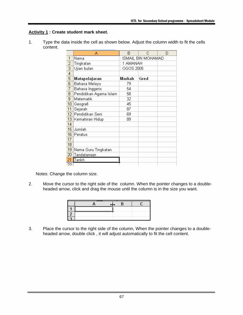
Activity 1 : Create student mark sheet. 1. Type the data inside the cell as shown below. Adjust the column width to fit the cells
content.
Notes: Change the column size. 2. Move the cursor to the right side of the column. When the pointer changes to a double-
headed arrow, click and drag the mouse until the column is in the size you want.
3. Place the cursor to the right side of the column, When the pointer changes to a double-
headed arrow, double click , it will adjust automatically to fit the cell content.
ICTL for Secondary School programme - Spreadsheet Module
68
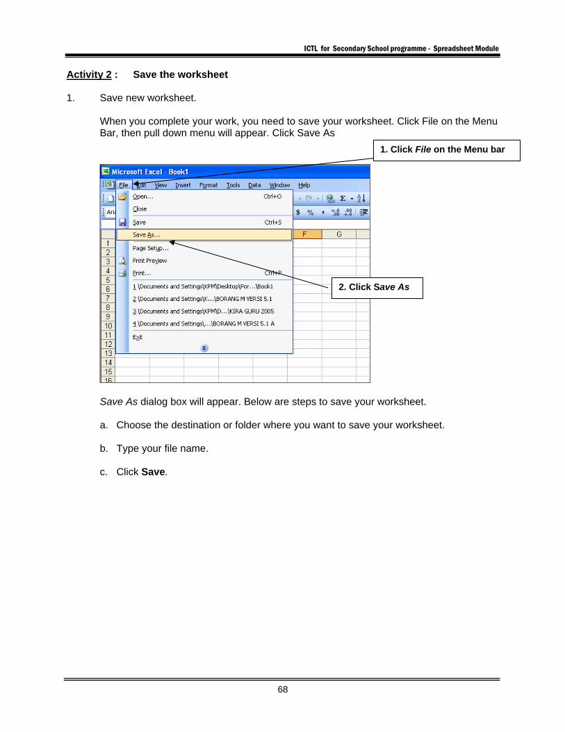
Activity 2 : Save the worksheet 1. Save new worksheet.
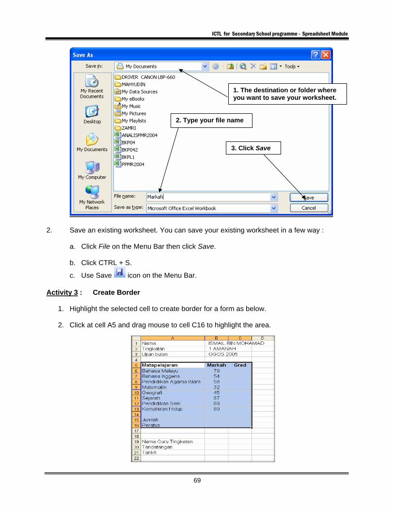
When you complete your work, you need to save your worksheet. Click File on the Menu Bar, then pull down menu will appear. Click Save As
Save As dialog box will appear. Below are steps to save your worksheet. a. Choose the destination or folder where you want to save your worksheet. b. Type your file name. c. Click Save.
1. Click File on the Menu bar
2. Click Save As
ICTL for Secondary School programme - Spreadsheet Module
69
2. Save an existing worksheet. You can save your existing worksheet in a few way :
a. Click File on the Menu Bar then click Save.
b. Click CTRL + S.
c. Use Save icon on the Menu Bar. Activity 3 : Create Border
1. Highlight the selected cell to create border for a form as below. 2. Click at cell A5 and drag mouse to cell C16 to highlight the area.
1. The destination or folder where you want to save your worksheet.
2. Type your file name
3. Click Save
ICTL for Secondary School programme - Spreadsheet Module
70
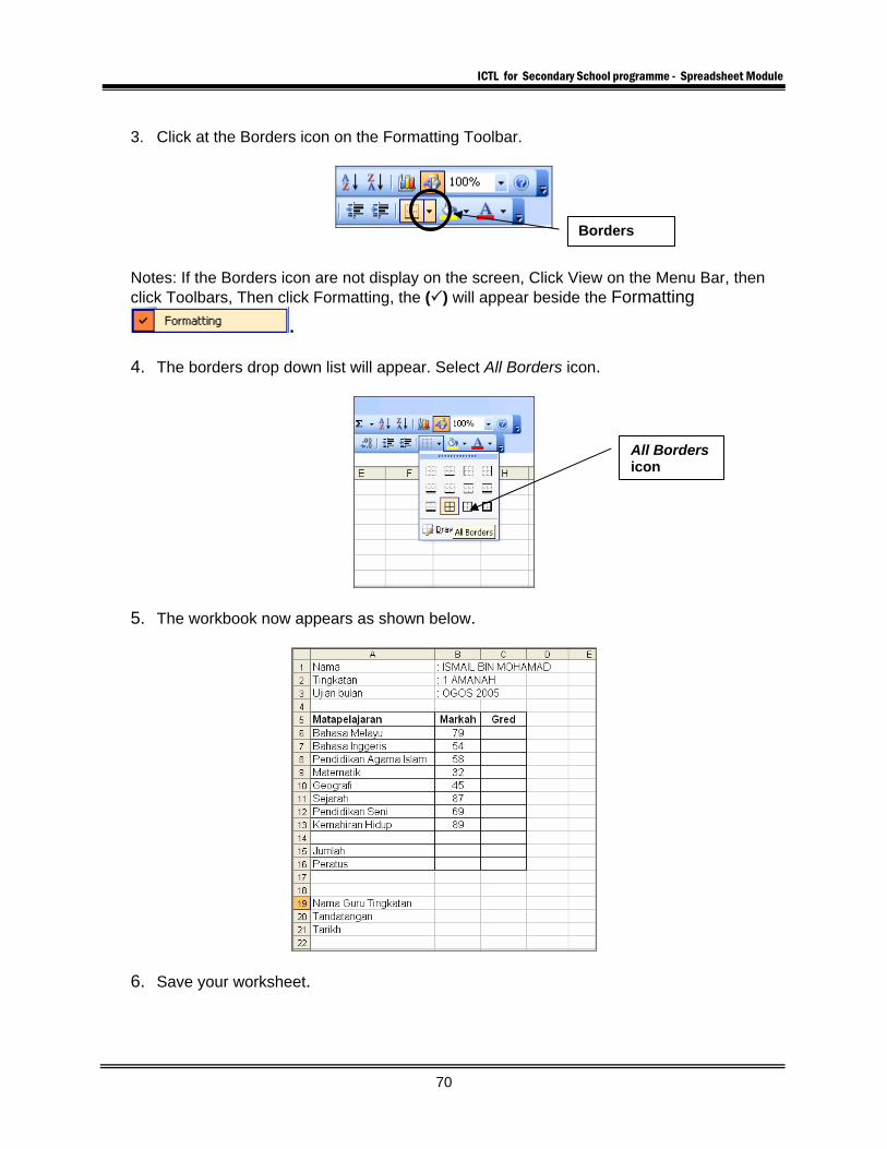
3. Click at the Borders icon on the Formatting Toolbar.
Notes: If the Borders icon are not display on the screen, Click View on the Menu Bar, then click Toolbars, Then click Formatting, the ( ) will appear beside the Formatting
. 4. The borders drop down list will appear. Select All Borders icon.
5. The workbook now appears as shown below.
6. Save your worksheet.
Borders
All Borders icon
ICTL for Secondary School programme - Spreadsheet Module
71
Activity 4: Insert formula
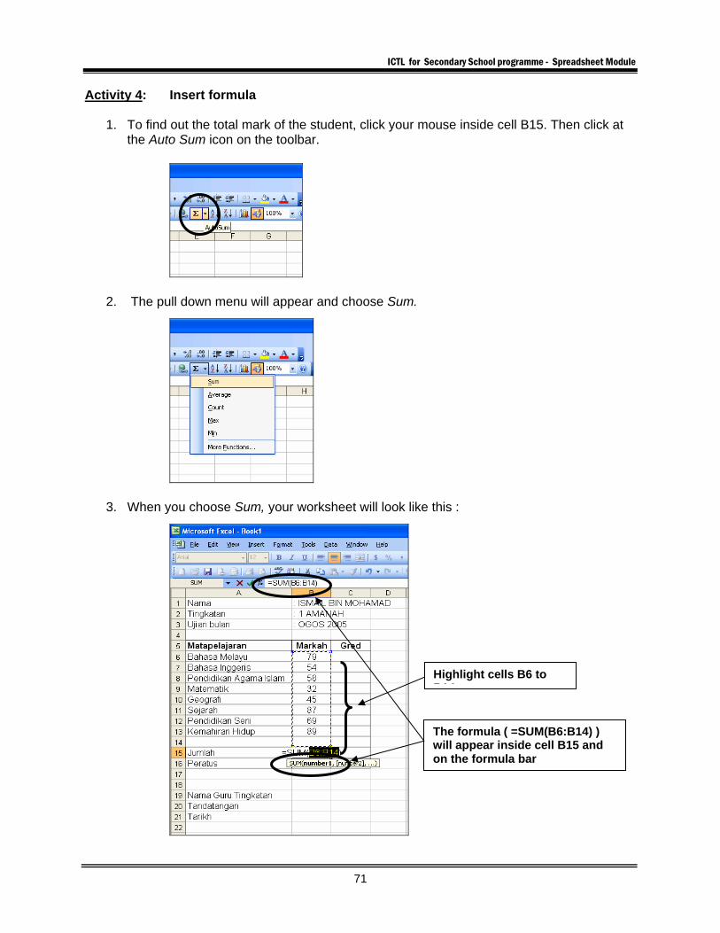
1. To find out the total mark of the student, click your mouse inside cell B15. Then click at the Auto Sum icon on the toolbar.
2. The pull down menu will appear and choose Sum.
3. When you choose Sum, your worksheet will look like this :
Highlight cells B6 to B14
The formula ( =SUM(B6:B14) ) will appear inside cell B15 and on the formula bar
ICTL for Secondary School programme - Spreadsheet Module
72
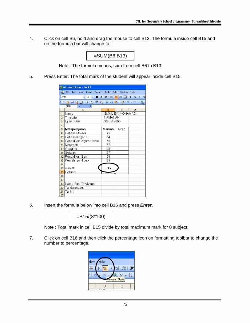
4. Click on cell B6, hold and drag the mouse to cell B13. The formula inside cell B15 and
on the formula bar will change to : Note : The formula means, sum from cell B6 to B13.
5. Press Enter. The total mark of the student will appear inside cell B15.
6. Insert the formula below into cell B16 and press Enter. Note : Total mark in cell B15 divide by total maximum mark for 8 subject. 7. Click on cell B16 and then click the percentage icon on formatting toolbar to change the
number to percentage.
=SUM(B6:B13)
=B15/(8*100)
ICTL for Secondary School programme - Spreadsheet Module
73
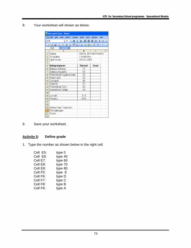
8. Your worksheet will shown as below.
9. Save your worksheet. Activity 5: Define grade 1. Type the number as shown below in the right cell. Cell E5: type 0 Cell E6: type 40 Cell E7: type 60 Cell E8: type 70 Cell E9: type 80 Cell F5: type E Cell F6: type D Cell F7: type C Cell F8: type B Cell F9: type A
ICTL for Secondary School programme - Spreadsheet Module
74
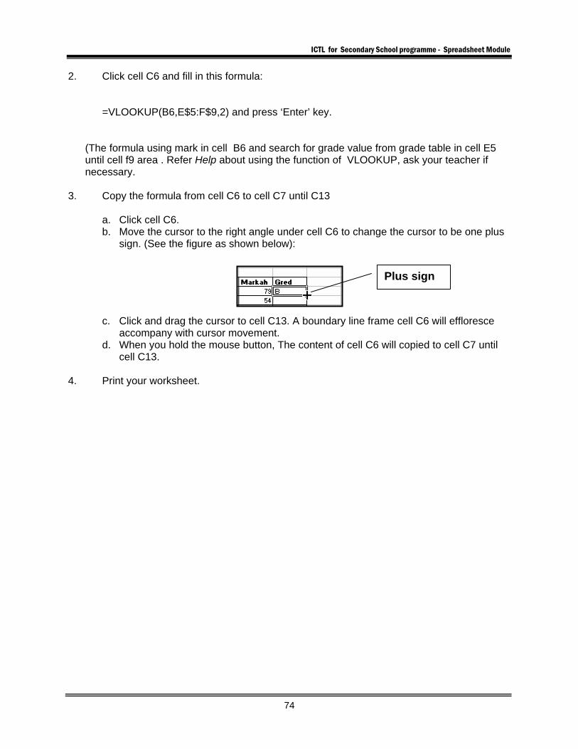
2. Click cell C6 and fill in this formula: =VLOOKUP(B6,E$5:F$9,2) and press ‘Enter’ key.
(The formula using mark in cell B6 and search for grade value from grade table in cell E5 until cell f9 area . Refer Help about using the function of VLOOKUP, ask your teacher if necessary.
3. Copy the formula from cell C6 to cell C7 until C13
a. Click cell C6. b. Move the cursor to the right angle under cell C6 to change the cursor to be one plus
sign. (See the figure as shown below):
c. Click and drag the cursor to cell C13. A boundary line frame cell C6 will effloresce accompany with cursor movement.
d. When you hold the mouse button, The content of cell C6 will copied to cell C7 until cell C13.
4. Print your worksheet.
Plus sign

ICTL for Secondary School programme - Spreadsheet Module
75
Activity 6: Produce the mark form of class monthly test In the Microsoft Excel, a workbook can content more than one sheet. In the activities before, you had produced an individual mark form in sheet 1 your sheet. For the mark foam of class monthly test, use a new sheet 1. Click the icon Sheet2 under your worksheet (The figure is appear ). A new sheet will appear. 2. To change orientation a page from Portrait to Landscape.
a. Click File on menu bar and a menu will appear as shown as below.
ICTL for Secondary School programme - Spreadsheet Module
76
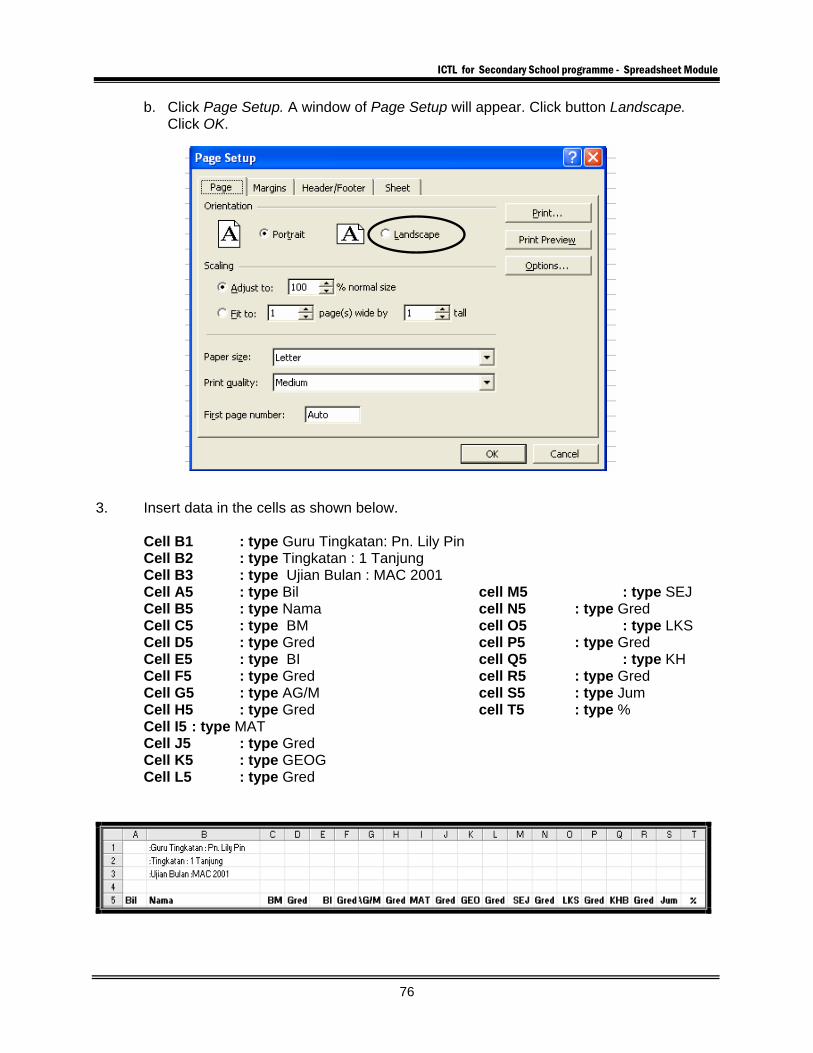
b. Click Page Setup. A window of Page Setup will appear. Click button Landscape. Click OK.
3. Insert data in the cells as shown below.
Cell B1 : type Guru Tingkatan: Pn. Lily Pin Cell B2 : type Tingkatan : 1 Tanjung Cell B3 : type Ujian Bulan : MAC 2001 Cell A5 : type Bil cell M5 : type SEJ Cell B5 : type Nama cell N5 : type Gred Cell C5 : type BM cell O5 : type LKS Cell D5 : type Gred cell P5 : type Gred Cell E5 : type BI cell Q5 : type KH Cell F5 : type Gred cell R5 : type Gred Cell G5 : type AG/M cell S5 : type Jum Cell H5 : type Gred cell T5 : type % Cell I5 : type MAT Cell J5 : type Gred Cell K5 : type GEOG Cell L5 : type Gred
ICTL for Secondary School programme - Spreadsheet Module
77
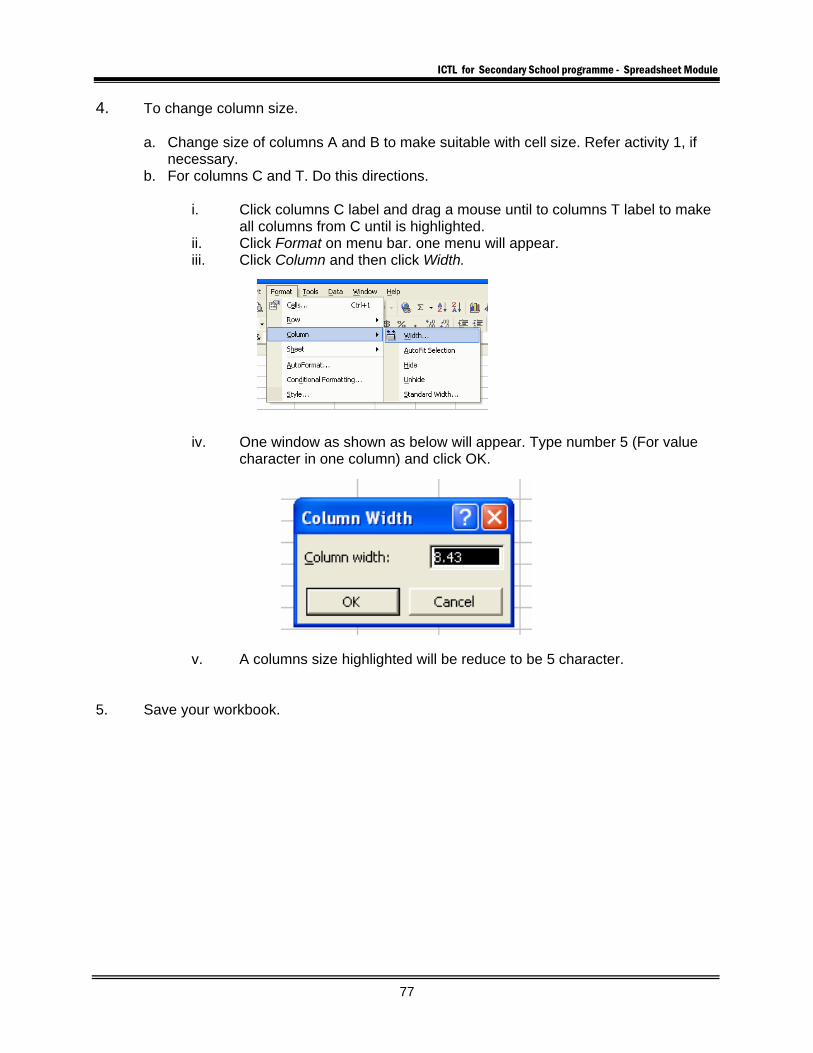
4. To change column size.
a. Change size of columns A and B to make suitable with cell size. Refer activity 1, if necessary.
b. For columns C and T. Do this directions.
i. Click columns C label and drag a mouse until to columns T label to make all columns from C until is highlighted.
ii. Click Format on menu bar. one menu will appear. iii. Click Column and then click Width. iv. One window as shown as below will appear. Type number 5 (For value
character in one column) and click OK.
v. A columns size highlighted will be reduce to be 5 character.
5. Save your workbook.
ICTL for Secondary School programme - Spreadsheet Module
78
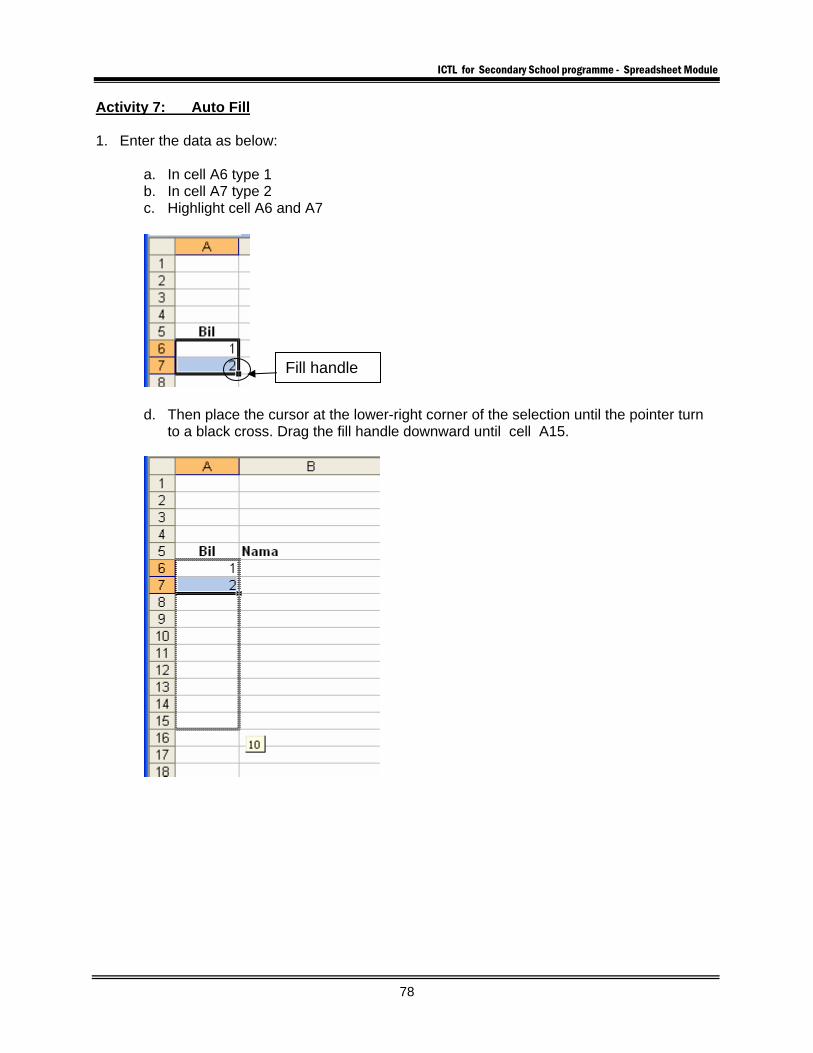
Activity 7: Auto Fill 1. Enter the data as below:
a. In cell A6 type 1 b. In cell A7 type 2 c. Highlight cell A6 and A7
d. Then place the cursor at the lower-right corner of the selection until the pointer turn
to a black cross. Drag the fill handle downward until cell A15.
Fill handle
ICTL for Secondary School programme - Spreadsheet Module
79
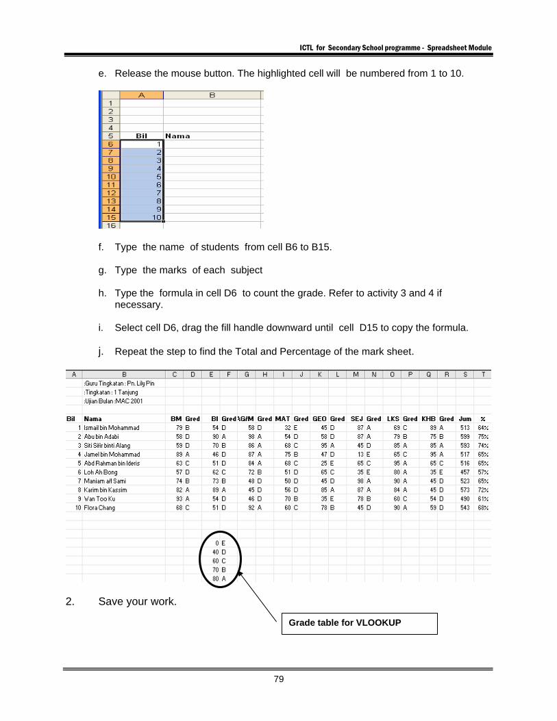
e. Release the mouse button. The highlighted cell will be numbered from 1 to 10.
f. Type the name of students from cell B6 to B15. g. Type the marks of each subject h. Type the formula in cell D6 to count the grade. Refer to activity 3 and 4 if
necessary. i. Select cell D6, drag the fill handle downward until cell D15 to copy the formula. j. Repeat the step to find the Total and Percentage of the mark sheet.
2. Save your work.
Grade table for VLOOKUP
ICTL for Secondary School programme - Spreadsheet Module
80
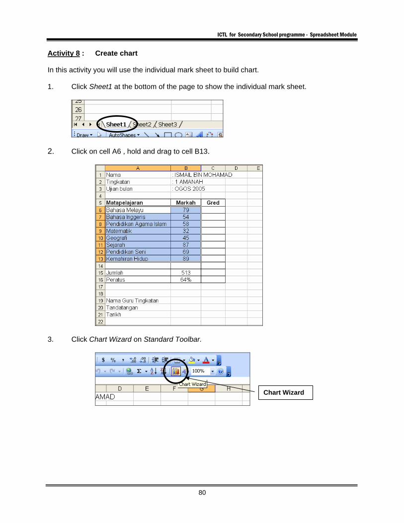
Activity 8 : Create chart In this activity you will use the individual mark sheet to build chart. 1. Click Sheet1 at the bottom of the page to show the individual mark sheet.
2. Click on cell A6 , hold and drag to cell B13.
3. Click Chart Wizard on Standard Toolbar.
Chart Wizard
ICTL for Secondary School programme - Spreadsheet Module
81
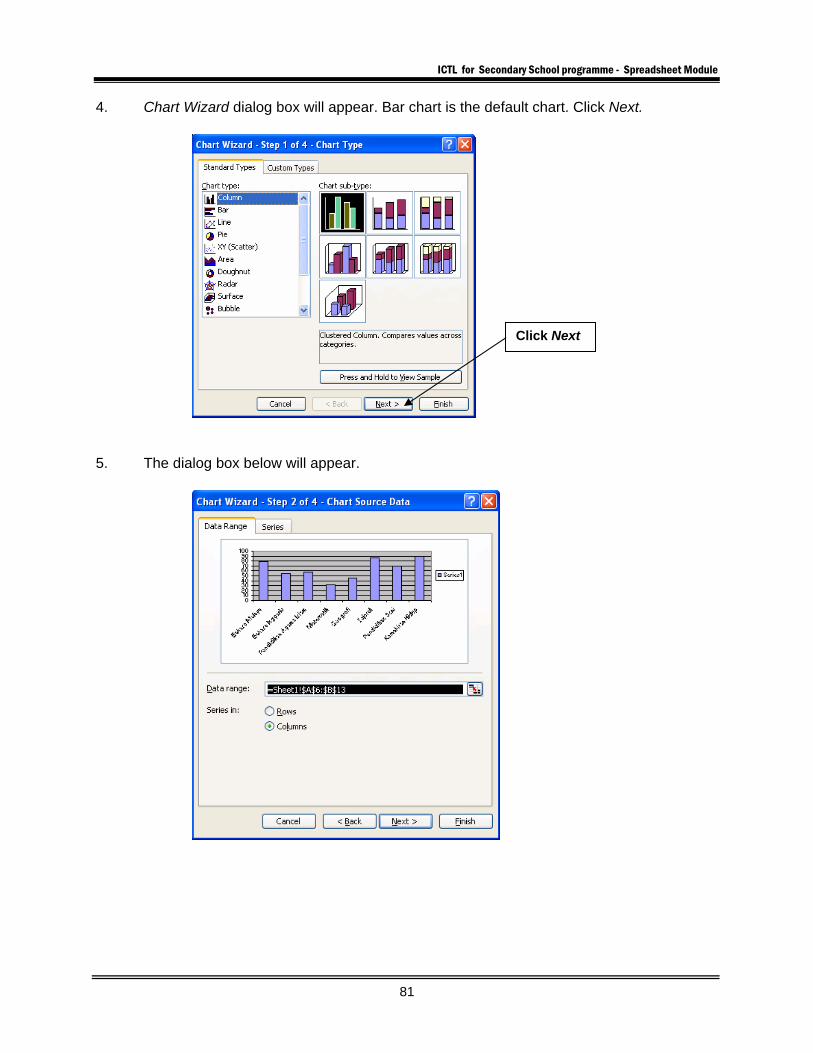
4. Chart Wizard dialog box will appear. Bar chart is the default chart. Click Next.
5. The dialog box below will appear.
Click Next
ICTL for Secondary School programme - Spreadsheet Module
82
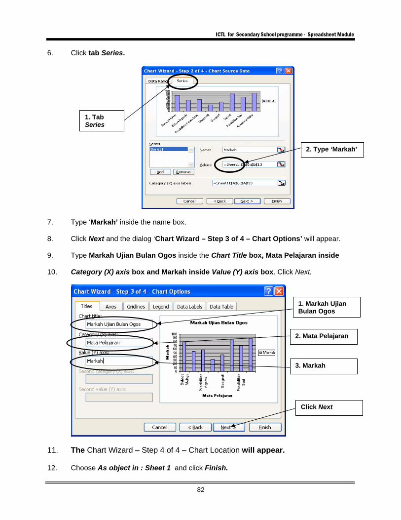
6. Click tab Series.
7. Type ‘Markah’ inside the name box. 8. Click Next and the dialog ‘Chart Wizard – Step 3 of 4 – Chart Options’ will appear. 9. Type Markah Ujian Bulan Ogos inside the Chart Title box, Mata Pelajaran inside 10. Category (X) axis box and Markah inside Value (Y) axis box. Click Next.
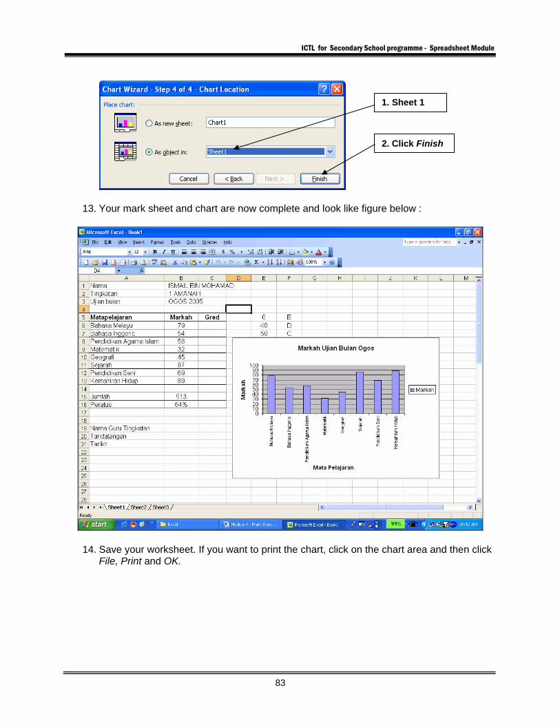
11. The Chart Wizard – Step 4 of 4 – Chart Location will appear.
12. Choose As object in : Sheet 1 and click Finish.
1. Tab Series
2. Type ‘Markah’
1. Markah Ujian Bulan Ogos
2. Mata Pelajaran
3. Markah
Click Next
ICTL for Secondary School programme - Spreadsheet Module
83
13. Your mark sheet and chart are now complete and look like figure below :
14. Save your worksheet. If you want to print the chart, click on the chart area and then click File, Print and OK.
1. Sheet 1
2. Click Finish
ICTL for Secondary School programme - Spreadsheet Module
84
MODULE 5
CREATING CHART
Curriculum Development Centre Ministry of Education Malaysia
ICTL for Secondary School programme - Spreadsheet Module
85
Name of Module : Creating Chart Learning Outcomes: The students should be able to:
1) Key in data into worksheet 2) Insert a chart in worksheet 3) Change chart type and properties 4) Close and exit workbook
Knowledge and Skills:
a) Create charts. b) Change chart type c) Change chart properties d) Delete charts e) Preview charts f) Print charts g) Save charts
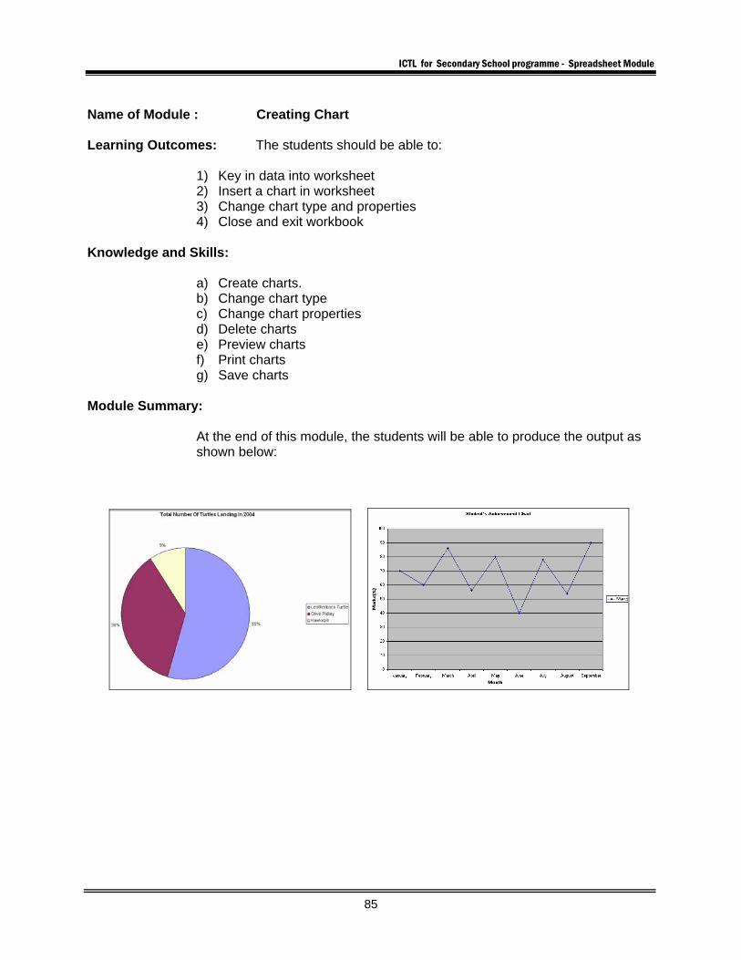
Module Summary:
At the end of this module, the students will be able to produce the output as shown below:
ICTL for Secondary School programme - Spreadsheet Module
86
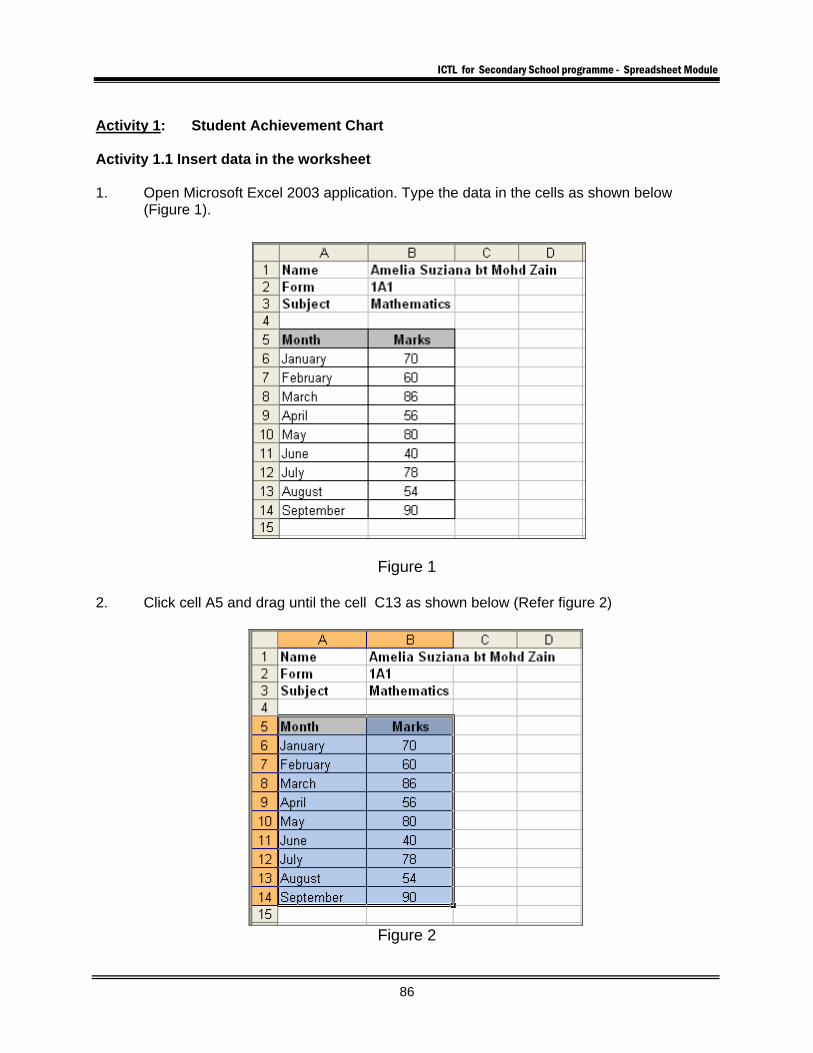
Activity 1: Student Achievement Chart Activity 1.1 Insert data in the worksheet 1. Open Microsoft Excel 2003 application. Type the data in the cells as shown below
(Figure 1).
Figure 1 2. Click cell A5 and drag until the cell C13 as shown below (Refer figure 2)
Figure 2
ICTL for Secondary School programme - Spreadsheet Module
87
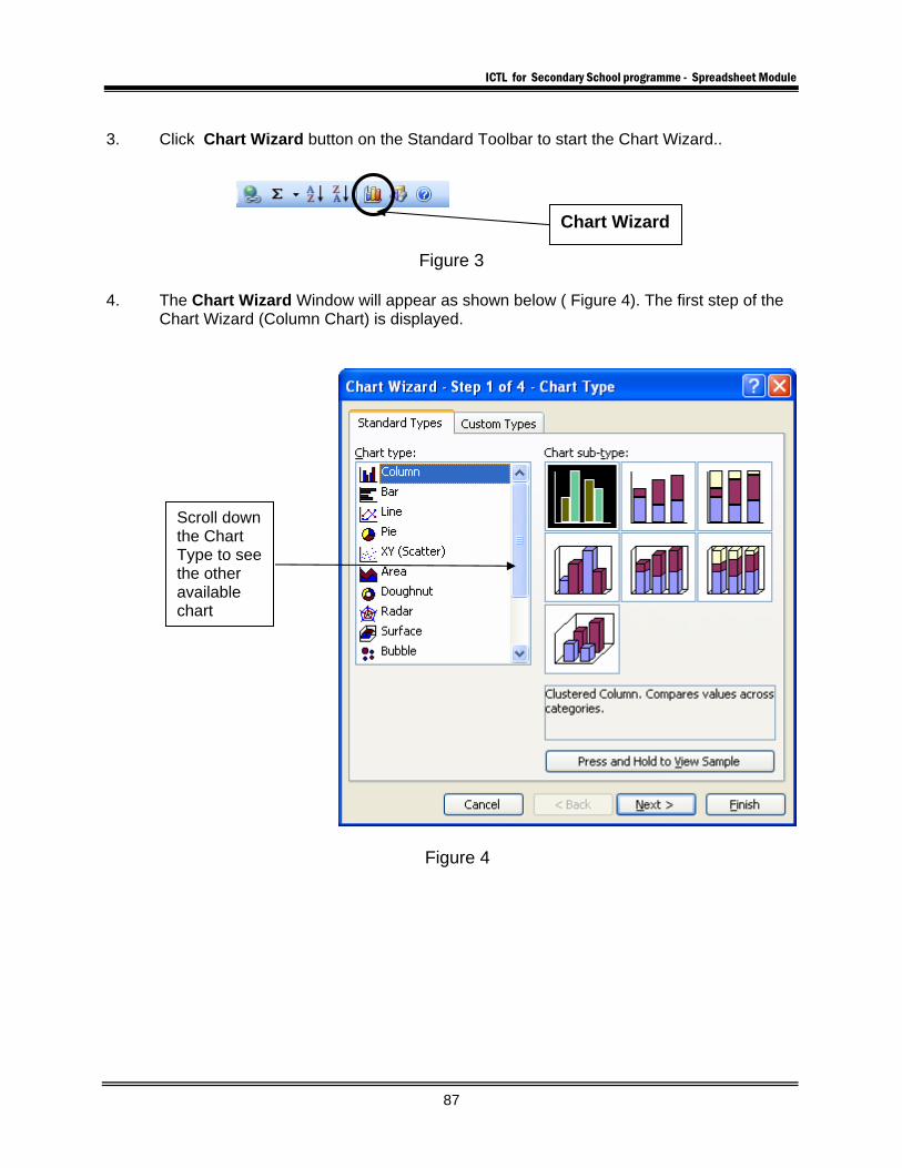
3. Click Chart Wizard button on the Standard Toolbar to start the Chart Wizard..
Figure 3
4. The Chart Wizard Window will appear as shown below ( Figure 4). The first step of the Chart Wizard (Column Chart) is displayed.
Figure 4
Scroll down the Chart Type to see the other available chart
Chart Wizard
ICTL for Secondary School programme - Spreadsheet Module
88
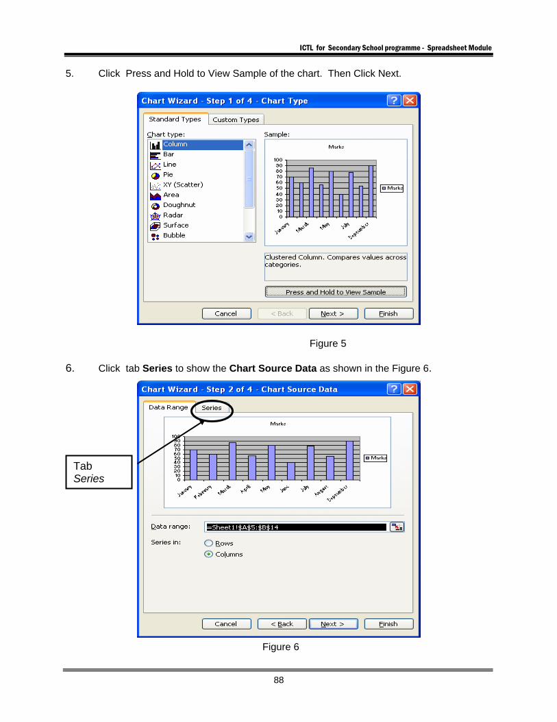
5. Click Press and Hold to View Sample of the chart. Then Click Next.
Figure 5 6. Click tab Series to show the Chart Source Data as shown in the Figure 6.
Figure 6
Tab Series
ICTL for Secondary School programme - Spreadsheet Module
89
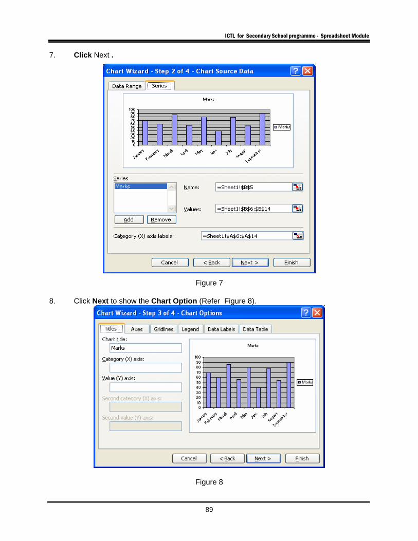
7. Click Next .
Figure 7
8. Click Next to show the Chart Option (Refer Figure 8).
Figure 8

ICTL for Secondary School programme - Spreadsheet Module
90
9. The default Chart Title (your first column header) will appear on Chart Options menu as
shown in Figure 8. 10. Change the Chart Title to Student Achievement Chart .Type the (X) axis and (Y) axis
Value as shown in Figure 9.
Figure 9 11. Click Next. Then Chart Location Dialog Box will appear as shown below (Figure 10). Set
the option button to place the chart As object in Sheet 1.
Figure 10
ICTL for Secondary School programme - Spreadsheet Module
91
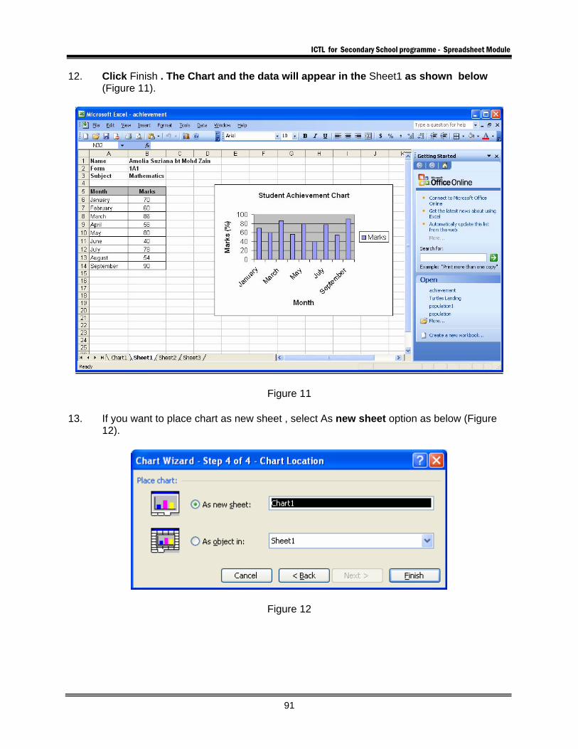
12. Click Finish . The Chart and the data will appear in the Sheet1 as shown below (Figure 11).
Figure 11 13. If you want to place chart as new sheet , select As new sheet option as below (Figure
12).
Figure 12

ICTL for Secondary School programme - Spreadsheet Module
92
14. Click Finish . The Chart will appear as Chart1 (Figure 13).
Figure 13
15. Save your worksheet as achieve.xls in your on Folder.
16. To print the Chart, highlight the Chart . Then Click File, Print
17. Click OK. Then close your worksheet.
ICTL for Secondary School programme - Spreadsheet Module
93
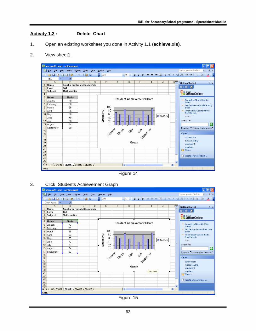
Activity 1.2 : Delete Chart 1. Open an existing worksheet you done in Activity 1.1 (achieve.xls). 2. View sheet1.
Figure 14
3. Click Students Achievement Graph
Figure 15
ICTL for Secondary School programme - Spreadsheet Module
94
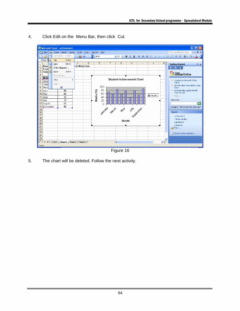
4. Click Edit on the Menu Bar, then click Cut.
Figure 16
5. The chart will be deleted. Follow the next activity.
ICTL for Secondary School programme - Spreadsheet Module
95
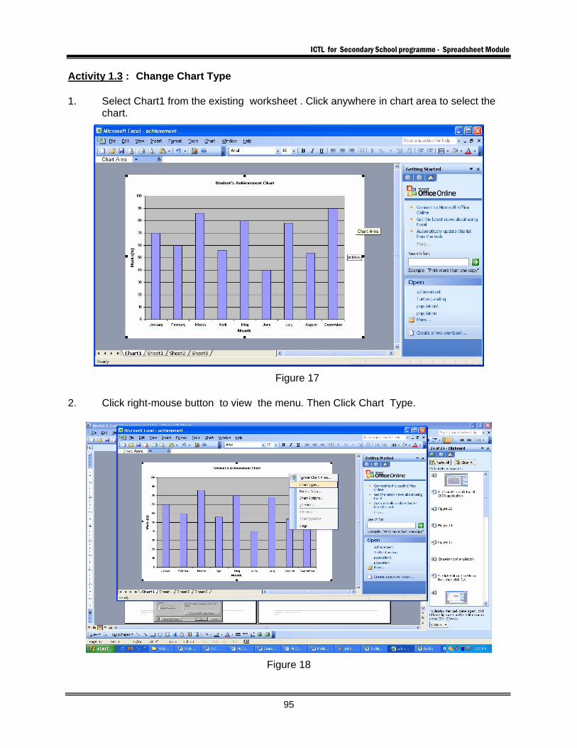
Activity 1.3 : Change Chart Type 1. Select Chart1 from the existing worksheet . Click anywhere in chart area to select the
chart.
Figure 17 2. Click right-mouse button to view the menu. Then Click Chart Type.
Figure 18
ICTL for Secondary School programme - Spreadsheet Module
96
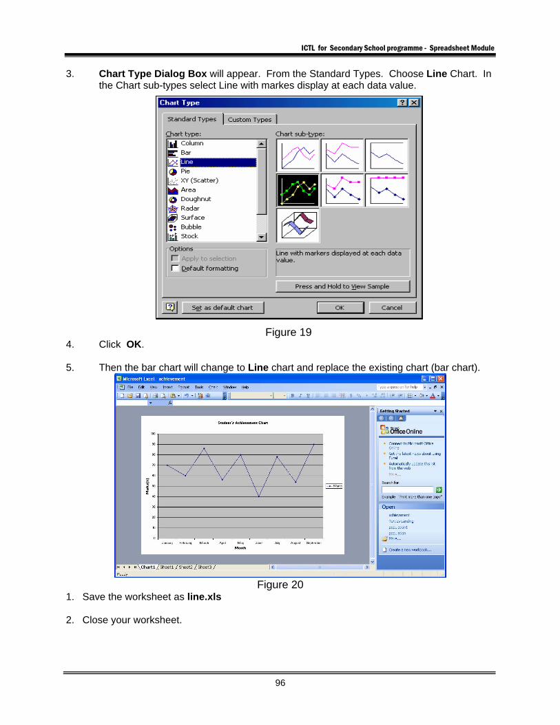
3. Chart Type Dialog Box will appear. From the Standard Types. Choose Line Chart. In the Chart sub-types select Line with markes display at each data value.
Figure 19 4. Click OK.
5. Then the bar chart will change to Line chart and replace the existing chart (bar chart).
Figure 20
1. Save the worksheet as line.xls 2. Close your worksheet.
ICTL for Secondary School programme - Spreadsheet Module
97
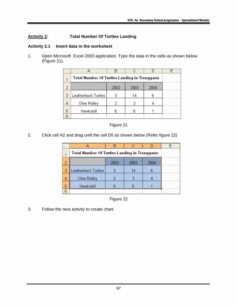
Activity 2: Total Number Of Turtles Landing Activity 2.1 Insert data in the worksheet 1. Open Microsoft Excel 2003 application. Type the data in the cells as shown below
(Figure 21).
Figure 21 2. Click cell A2 and drag until the cell D5 as shown below (Refer figure 22)
Figure 22
3. Follow the next activity to create chart.

ICTL for Secondary School programme - Spreadsheet Module
98
Activity 2.2 Stacked column with a 3-D visual effect 1. Click Chart Wizard button on the Standard Toolbar to start the Chart Wizard..
Figure 23 2. The Chart Wizard Window will appear as shown below ( Figure 4). The first step of the
Chart Wizard (Column Chart) is displayed.
Figure 24
Chart Wizard
Scroll down the Chart Type to see the other available chart
ICTL for Secondary School programme - Spreadsheet Module
99
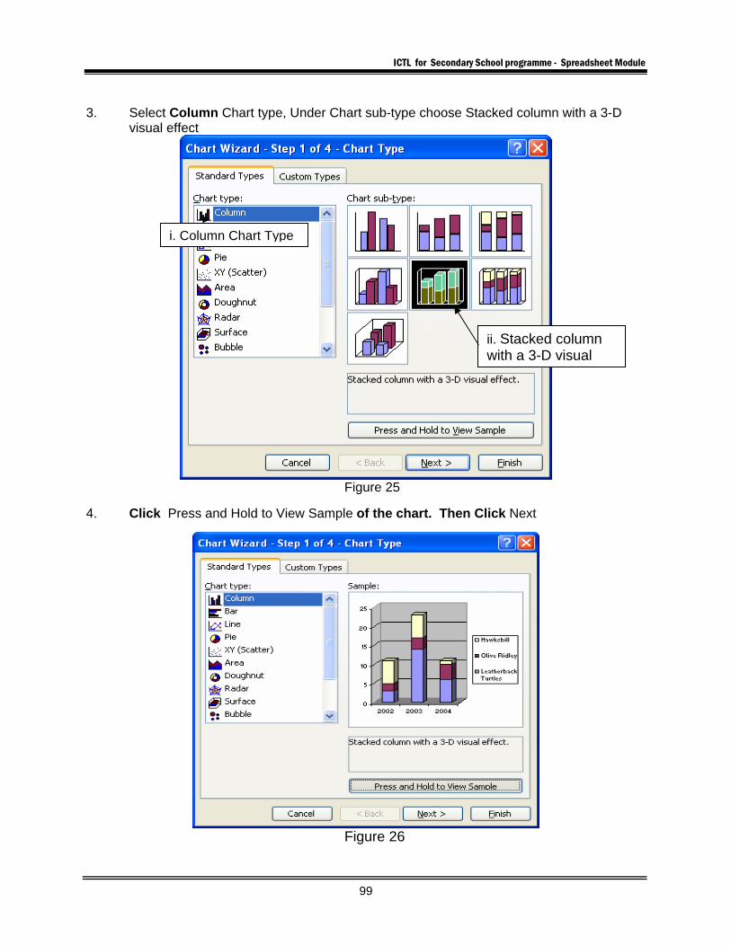
3. Select Column Chart type, Under Chart sub-type choose Stacked column with a 3-D
visual effect
Figure 25
4. Click Press and Hold to View Sample of the chart. Then Click Next
Figure 26
i. Column Chart Type
ii. Stacked column with a 3-D visual
ICTL for Secondary School programme - Spreadsheet Module
100
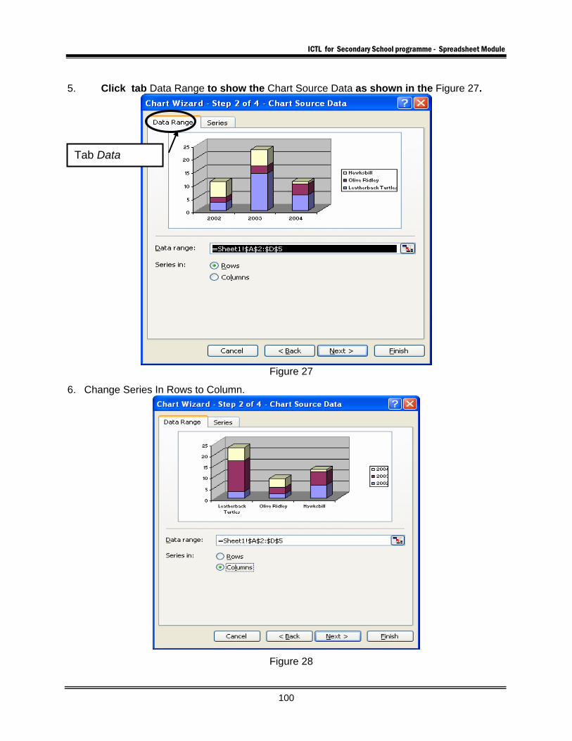
5. Click tab Data Range to show the Chart Source Data as shown in the Figure 27.
Figure 27
6. Change Series In Rows to Column.
Figure 28
Tab Data
ICTL for Secondary School programme - Spreadsheet Module
101
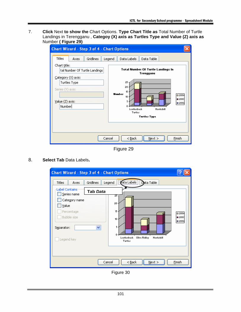
7. Click Next to show the Chart Options. Type Chart Title as Total Number of Turtle Landings in Terengganu , Categoy (X) axis as Turtles Type and Value (Z) axis as Number ( Figure 29)
Figure 29 8. Select Tab Data Labels.
Figure 30
Tab Data
ICTL for Secondary School programme - Spreadsheet Module
102
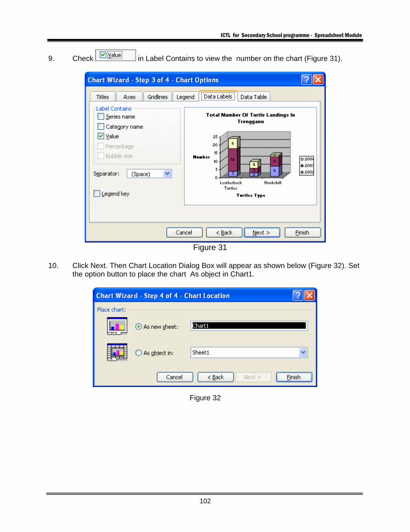
9. Check in Label Contains to view the number on the chart (Figure 31).
Figure 31
10. Click Next. Then Chart Location Dialog Box will appear as shown below (Figure 32). Set
the option button to place the chart As object in Chart1.
Figure 32
ICTL for Secondary School programme - Spreadsheet Module
103
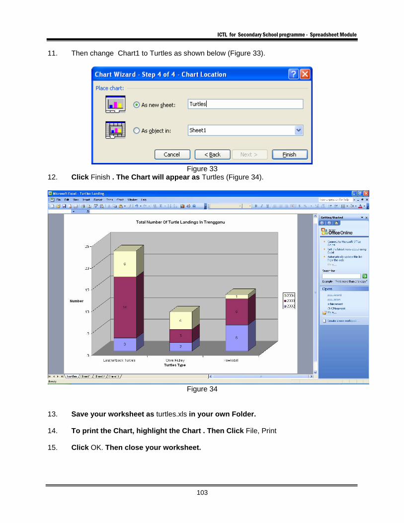
11. Then change Chart1 to Turtles as shown below (Figure 33).
Figure 33
12. Click Finish . The Chart will appear as Turtles (Figure 34).
Figure 34
13. Save your worksheet as turtles.xls in your own Folder. 14. To print the Chart, highlight the Chart . Then Click File, Print 15. Click OK. Then close your worksheet.
ICTL for Secondary School programme - Spreadsheet Module
104
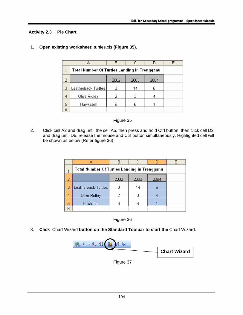
Activity 2.3 Pie Chart 1. Open existing worksheet: turtles.xls (Figure 35).
Figure 35
2. Click cell A2 and drag until the cell A5, then press and hold Ctrl button, then click cell D2 and drag until D5, release the mouse and Ctrl button simultaneously. Highlighted cell will be shown as below (Refer figure 36)
Figure 36
3. Click Chart Wizard button on the Standard Toolbar to start the Chart Wizard.
Figure 37
Chart Wizard
ICTL for Secondary School programme - Spreadsheet Module
105
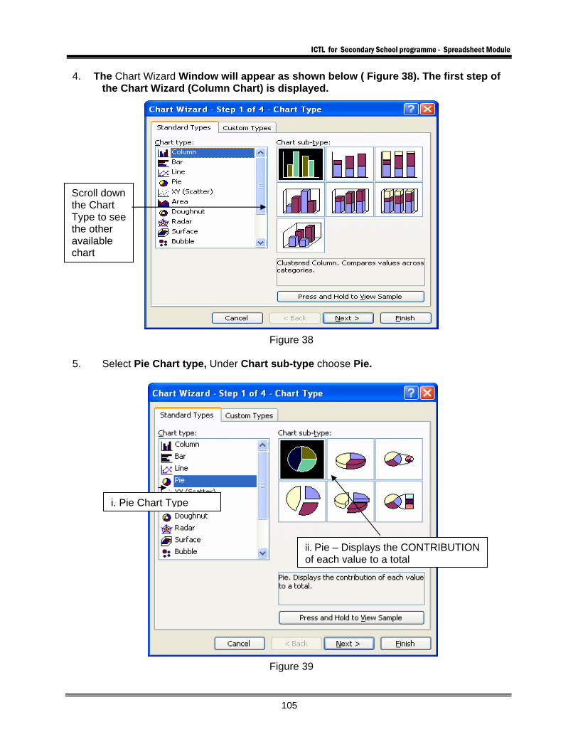
4. The Chart Wizard Window will appear as shown below ( Figure 38). The first step of the Chart Wizard (Column Chart) is displayed.
Figure 38 5. Select Pie Chart type, Under Chart sub-type choose Pie.
Figure 39
Scroll down the Chart Type to see the other available chart
i. Pie Chart Type
ii. Pie – Displays the CONTRIBUTION of each value to a total
ICTL for Secondary School programme - Spreadsheet Module
106
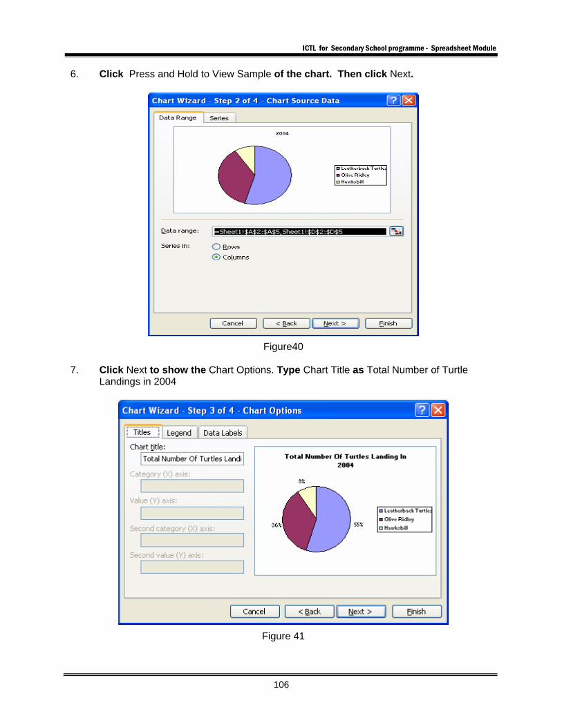
6. Click Press and Hold to View Sample of the chart. Then click Next.
Figure40 7. Click Next to show the Chart Options. Type Chart Title as Total Number of Turtle
Landings in 2004
Figure 41
ICTL for Secondary School programme - Spreadsheet Module
107
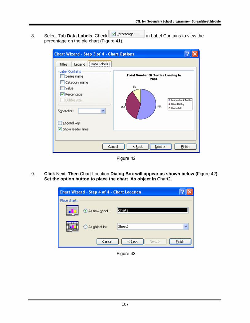
8. Select Tab Data Labels. Check in Label Contains to view the percentage on the pie chart (Figure 41).
Figure 42
9. Click Next. Then Chart Location Dialog Box will appear as shown below (Figure 42). Set the option button to place the chart As object in Chart2.
Figure 43
ICTL for Secondary School programme - Spreadsheet Module
108
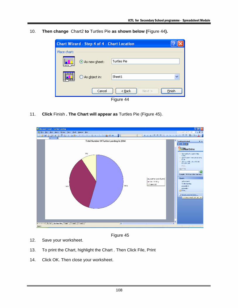
10. Then change Chart2 to Turtles Pie as shown below (Figure 44).
Figure 44
11. Click Finish . The Chart will appear as Turtles Pie (Figure 45).
Figure 45 12. Save your worksheet. 13. To print the Chart, highlight the Chart . Then Click File, Print 14. Click OK. Then close your worksheet.
ICTL for Secondary School programme - Spreadsheet Module
109
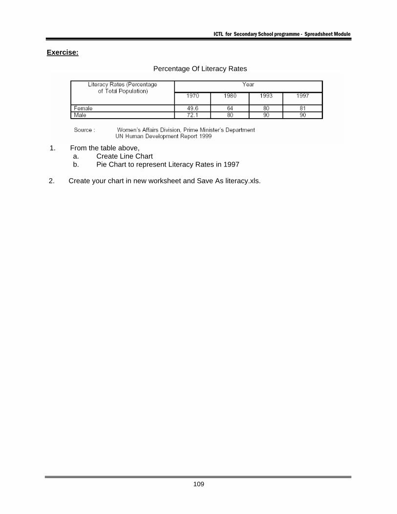
Exercise:
Percentage Of Literacy Rates
1. From the table above,
a. Create Line Chart b. Pie Chart to represent Literacy Rates in 1997
2. Create your chart in new worksheet and Save As literacy.xls.