seasonal - ecb.europa.eu · seasonal patterns and trading-day effects where relevant. ... seasonal...
TRANSCRIPT

SeasonalAdjustment
Sea
sona
l Adj
ustm
ent
EURO
PEA
N C
ENT
RA
L BA
NK
Titel_16182.pmd 12.11.03, 07:331

SeasonalAdjustment
Editors:
Michele Manna and Romana Peronaci

Published by:© European Central Bank, November 2003
Address Kaiserstrasse 2960311 Frankfurt am MainGermany
Postal address Postfach 16 03 1960066 Frankfurt am MainGermany
Telephone +49 69 1344 0
Internet http://www.ecb.int
Fax +49 69 1344 6000
Telex 411 144 ecb d
This publication is also available as an e-book to be downloaded from the ECB’s website.
The views expressed in this publication do not necessarily reflect those of the European Central Bank.No responsibility for them should be attributed to the ECB or to any of the other institutions with whichthe authors are affiliated.
All rights reserved by the authors.
Editors:Michele Manna and Romana Peronaci
Typeset and printed by:Kern & Birner GmbH + Co.As at January 2003.
ISBN 92-9181-412-1 (print)ISBN 92-9181-413-X (online)

Contents
Foreword by Eugenio Domingo Solans ........................................................................ 5
Notes from the Chairman Michele Manna ..................................................................... 7
1 Comparing direct and indirect seasonal adjustments of aggregate seriesby Catherine C. Hood and David F. Findley .............................................................. 9
2 A class of diagnostics in the ARIMA-model-based decomposition of a time series by Agustín Maravall ............................................................................... 23
3 Seasonal adjustment of European aggregates: direct versus indirect approachby Dominique Ladiray and Gian Luigi Mazzi ........................................................... 37
4 Criteria to determine the optimal revision policy: a case study based oneuro zone monetary aggregates data by Laurent Maurin ....................................... 67
5 Direct versus indirect seasonal adjustment of UK monetary statistics:preliminary discussion by David Willoughby ......................................................... 85
6 The seasonal adjustment of euro area monetary aggregates:direct versus indirect approach by Romana Peronaci ............................................ 91
7 Monthly re-estimation of the parameters of a once-a-year fixed model:an assessment by Soledad Bravo Cabría, Coral García Esteban andAntonio Montesinos Afonso ...................................................................................... 109
8 Seasonal adjustment quality reports by Stefano Nardelli ..................................... 127
9 The performance of X-12 in the seasonal adjustment of short time seriesby Antonio Matas Mir and Vitaliana Rondonotti ....................................................... 149
Seminar agenda ............................................................................................................ 161

4 Contents

Foreword
The main objective of the European Central Bank is the maintenance of price stability over themedium term. The challenge faced by central banks is that monetary policy decisions takentoday will affect the price level only in the future. The ECB’s monetary policy strategy aims toensure that the Governing Council receives all the relevant statistics, analysis and additionalinformation to take the monetary policy decisions needed today in order to maintain pricestability over the medium term. The strategy assigns a prominent role to money. In the longrun, the relationship between money and the price level is stable, especially when money ismeasured using broad monetary aggregates such as M3. In the short run, however, monetarydevelopments may be subject to special influences and distortions, which make forward-looking monetary policy decisions more complex. The monetary analysis of the ECB intendsto filter the underlying long-term relationship in the statistics from repercussions by short-term effects. One main approach is the seasonal adjustment of monetary and economicstatistics. Seasonally adjusted data allows monitoring short-term developments irrespective ofseasonal patterns and trading-day effects where relevant.
Each month, the ECB derives seasonally adjusted results for the principal euro areamonetary aggregates and counterparts. In addition, in collaboration with the EuropeanCommission (Eurostat, the Statistical Office of the European Communities), it producesseasonally adjusted measures of a wide range of other real economy and price statistics for theeuro area, including the Harmonised Index of Consumer Prices (HICP) and GDP.
The compilation of seasonally adjusted data for the euro area implies some challenges,because the concept of a “euro area” is new and harmonised euro area statistics only availablefor a short period of time and a limited set of indicators. Of particular interest in the context ofeuro area statistics is the discussion of “direct” versus “indirect” seasonal adjustment.Advantages and drawbacks of a direct adjustment of euro area results as compared to anindirect adjustment via the aggregation of seasonally adjusted sub-components such ascountry results, need to be carefully considered.
The ECB organised this one-day seminar to bring together professionals in the area ofseasonal adjustment from central banks and statistical offices. The exchange of ideasstimulates further theoretical and practical work in seasonal adjustment, which would be ofbenefit for the monetary and economic analysis of the ECB.
Frankfurt am Main, November 2002
Eugenio Domingo SolansMember of the Executive Board of the European Central Bank

6

Note from the Chairman
Michele Manna
Seasonal adjustment plays a central role in the set-up of the statistical basis used by decision-makers to assess the economic outlook. Seasonally adjusted data are one of the tools used bythe ECB to measure the growth of its key monetary aggregate M3. Likewise, the EUstatistical office, Eurostat, gives priority to seasonally adjusted data in communicating thegrowth of euro area GDP, as do the US Federal Reserve (in respect of its index of industrialproduction) and the US Bureau of Economic Analysis (as regards the US GDP).
At the same time, seasonal adjustment receives comparatively limited attention fromacademic researchers. A search in the database Helecon International returned 35 entries for“seasonal adjustment”, while two other terms applicable to time series interpolationtechniques, “trend cycle” and “trend estimates”, had 306 and 257 entries respectively.
It was thus with a view to reflecting on the needs of both official producers of statistics andacademic researchers that on 12 November 2002 the ECB’s Money and Banking StatisticsDivision organised a one-day seminar on the subject of seasonal adjustment. The seminarinvolved presentations and discussions by staff members from the ECB, EU and accessioncountry central banks, the US Census Bureau and Eurostat.
When should a researcher judge the seasonal adjustment of a time series to be adequate? Inother words, when has the seasonal component been sufficiently whitened so that no seasonaleffect can be detected in the seasonally adjusted series? Already at this rather general level,the researcher faces a number of highly empirical issues. For example, the question arises ofwhether one should adjust directly the series under examination, or rather proceed indirectly,by first adjusting some sub-components and then aggregating. Moreover, the producer ofadjusted statistics must tackle the issue of the optimal frequency of review of the seasonalmodels/parameters/factors. It is also of interest for the expert in the field to monitor thedevelopments in the two main paradigms used in the industry, X12-REGARIMA andTRAMO/SEATS. Finally, further light should be shed on the properties of the seasonaladjustment estimates of short time series.
The discussion at the seminar revolved around these themes. Please refer to the papers fora thorough presentation. I should like here to flag some of the main results which arenoteworthy for their general applicability, both within and outside the field of statisticiansworking in central banks or statistical institutes. I hope I can do justice to the efforts made bythe authors.
First and foremost, it can never be emphasised enough that there is no fundamental reasonwhy a seasonally adjusted series should be smooth. This reflects the fact that the irregularcomponent is an integral part of the seasonally adjusted series.
Second, in addition to the visual inspection of the spectrum, the researcher can rely on aclass of tests to assess the under/overestimation of the seasonality, and the stability of theseasonal components. In this respect, as a good rule of thumb, it should be borne in mind thatwhen the seasonality of the series is very stable, with little stochastic variation, the filter mayover-adjust (remove too much variation as seasonal), and vice versa.
Third, as to the issue of direct versus indirect adjustment, empirical work undertaken onbroad sets of time series provides only mixed evidence on which of the two approaches issuperior to the other. The applied researcher may, however, wish to note that the indirectadjustment tends to be more effective if the sub-components do not have similar time-seriesproperties or if their relative importance (in terms of weight) changes very rapidly. At the

8
same time, while neither of the two approaches systematically dominates the other, it is onlyunder rather restrictive conditions that the two approaches yield the same seasonally adjustedresults. In theory, the issue of the direct versus the indirect approach could be solved by meansof a system-based estimation. In practice, given its computational complexity and itsshortcomings with respect to revision errors, this approach has rarely been used, andunivariate approaches are generally preferred.
Fourth, as regards the optimal frequency of updating models/parameters/factors, it can beshown that frequent updates of the model do not necessarily improve the quality of seasonallyadjustment data. Same remark holds true in respect to the frequency of re-estimation of theseasonal factors. Conversely, the analyst avails of more degrees of freedom as regards theupdating of the parameters of the model.
Fifth, when seasonal adjustment is run on fairly short time series, e.g. five years of monthlydata, simulations point to serious distortions in the results for the first two years of the sample.Furthermore, when outliers occur at the beginning of a short time series, the distortionsintroduced may be very large compared with the situation in which additional past data areavailable. More generally, the use of longer series is particularly recommended when theseasonal component is highly volatile.
Sixth and finally, to quote Agustín Maravall, “While X12 provides a quality assessment ofthe estimated component […], the SEATS diagnostics provide specification-type tests […].Viewed in this way the information given by the two approaches can be seen ascomplementary.” It is in this light that work is ongoing to establish a facility integrating X12and TRAMO/SEATS.
In sum, I am convinced that the seminar provided the opportunity for a stimulatingexchange of ideas among professional economists and statisticians working on the seasonaladjustment of “official” time series. The outcome of this exchange was a good mix oftheoretical and applied results which I hope can also be of use outside the circle of expertsdealing with seasonal adjustment in central banks and statistical offices.
At this point, I should once again like to thank all those who participated in the seminar fortheir contributions, whether in the form of papers or active involvement in the discussion. Atthe ECB, I should like to express special thanks to Romana Peronaci and Helena Roland, whotook over most of the burden involved in the practical organisation of the seminar.
European Central BankFrankfurt am Main, November 2002

1
Comparing direct and indirect seasonal adjustmentsof aggregate series
Catherine C. Hood and David F. Findley
If a time series is a sum (or other composite) of component series that are seasonally adjusted,we can sum the seasonally adjusted component series to get an indirect adjustment for theaggregate series. This kind of adjustment is called an indirect adjustment of the aggregateseries. The alternative is the direct adjustment obtained by applying the seasonal adjustmentprocedure directly to the aggregate data. For example, when we seasonally adjust exportseries at the individual end-use-code level and then sum the adjustments to get Total Exports,we have an indirect adjustment of Total Exports. If we sum the individual series first to getTotal Exports and then seasonally adjust the total, we have a direct adjustment of TotalExports. Under most circumstances, the direct and indirect adjustments for an aggregateseries are not identical.
This paper discusses the methodological practices of adjusting aggregate series and thediagnostics we use at the U.S. Census Bureau to help us judge the quality of the adjustments,including indirect adjustments generated from two different seasonal adjustment programssuch as X-12-ARIMA and SEATS.
We will discuss attributes of an acceptable seasonal adjustment and how to look for signsof inadequacy in the adjustment, particularly with aggregate series. We will also discussbriefly some diagnostics for judging the quality of the adjustment, including smoothness andrevisions.
1. Methods
The Census Bureau uses its X-12-ARIMA software to produce seasonally adjusted numbers.X-12-ARIMA and its predecessors, X-11 and Statistics Canada’s X-11-ARIMA, are widely-used seasonal adjustment programs. One of the major improvements of X-12-ARIMA is itsadditional diagnostics. For more information, see Findley, Monsell, Bell, Otto and Chen(1998) or the X-12-ARIMA Reference Manual, Final Version 0.2 (U.S. Census Bureau 2002).
Different estimates of the seasonal effects in an economic time series can arise fromdifferent choices of the options in the seasonal adjustment software. Or, in an aggregateseries, different estimates can also result from different choices of the level of aggregation atwhich seasonal adjustment is performed.
Our larger aggregate series, such as Total Retail Sales, Total Value of Construction, TotalImports, and Total Exports, are seasonally adjusted indirectly. For any aggregate series that ispublished, staff at the Bureau also looks at the diagnostics for the aggregate’s seasonaladjustment.
For the U.S. Import and Export series, the Census Bureau publishes the monthly data, so welook at the diagnostics for the monthly seasonal adjustment. However, the data are also
This paper reports the results of research and analysis undertaken by Census Bureau staff. It has undergonea Census Bureau review more limited in scope than that given to official Census Bureau publications. Thisreport is released to inform interested parties of ongoing research and to encourage discussion of work inprogress.

10 Hood and Findley
summed to quarters and published quarterly elsewhere (based on our monthly seasonaladjustments), so we also look at diagnostics for the quarterly series and the quarterlyaggregates.
With regard to aggregate series, staff at the Census Bureau looks at the diagnostics for eachcomponent series to decide if the series is seasonal or not and to decide on the options toproduce the best possible seasonal adjustment. We look very carefully at every series todetermine if the series is seasonal and if it can be adjusted reliably. When deciding on the bestpossible options, if we have many series to look at in a short period of time, we focus on thelarger-valued series first.
2. Diagnostics for direct and indirect adjustments used atthe Census Bureau
Whether direct or indirect adjustment is better for a given set of series depends on the set ofseries in question (Dagum 1979; and Pfefferman, Salama, and Ben-Turvia 1984). Generallyspeaking, when the component series that make up the aggregate series have quite distinctseasonal patterns and have adjustments of good quality, indirect seasonal adjustment isusually of better quality than the direct adjustment. On the other hand, when the componentseries have similar seasonal patterns, then summing the series may result in noisecancellation, and the direct seasonal adjustment is usually of better quality than the indirectadjustment. How do we know if it’s better to use direct or indirect adjustment for a given setof series? How similar do the component series need to be in order for direct adjustments tobe of superior quality? If the component adjustments are acceptable, will the indirectadjustment always be acceptable as well? The best way to answer these questions is to look atthe diagnostics.
2.1 Features of a quality adjustment
The most fundamental requirement of a seasonal adjustment, regarding quality, is that therebe no estimable seasonal effect still present in the seasonally adjusted series or in thedetrended seasonally adjusted series (i.e., in the irregular component).
Other important qualities of a good adjustment are the lack of bias in the level of the seriesand the stability of the estimates. A lack of bias in the level means that the local level of theseries will be similar for both the original series and the seasonally adjusted series. Stabilityof the estimates means that as new data are added and incorporated into the estimationprocedure, the revisions to the past estimates are small. Large revisions can indicate that theoriginal estimates are misleading or even meaningless.
There are other features that may be desirable in an adjustment. Some users may prefer asmoother adjustment. However, it is important to remember that achieving such desiredfeatures can conflict with the quality requirements mentioned earlier. For example, thesmoother of two adjustments may also be the one that is more susceptible to large revisions asfuture data become available and are included in the adjustment calculations. Some users mayfind an adjustment with large revisions to be unsuitable. Analysis of seasonal adjustmentfilters shows that increased smoothing is often associated with great delay in detectingturning points (Findley, Martin, and Wills 2002), and delayed turning point detection may beunsuitable to users also. Therefore, it is important to balance all the qualities and featuresdesired.
It is important to always check the quality of the adjustment. This applies to the direct and

Comparing direct and indirect seasonal adjustments of aggregate series 11
indirect adjustments, as well as the adjustments of all the component series. We will giveexamples later in the paper to show the importance of diagnostics.
2.2 Diagnostics for residual seasonality
One of the most important diagnostics is the spectral diagnostic for residual seasonality andtrading day effects, examples of which will be given below. For series with at least 60observations, the Census Bureau encourages users to look at this diagnostic to see if there areany residual calendar effects.
The spectrum of an observed time series shows the strength, or amplitude, of eachfrequency component when the data are decomposed into such components. For a monthlyseries with a strong seasonal effect, the spectrum will have especially large amplitudes at thefrequencies associated with components that repeat every year, i.e., every twelve months,every six months, every three months, etc. Therefore, for monthly series with a strongseasonal effect, we will see peaks in the spectrum at frequencies k/12 cycles per month, for1 ≤ k ≤ 6. For a quarterly series with a strong seasonal effect, we will see peaks in thespectrum at the frequencies ¼ cycle per quarter and at ½ cycle per quarter. See also Findleyet al (1998).
With inadequate seasonal adjustments that contain residual seasonality, the residual effectsare usually rather weak, and it is necessary to remove any very strong frequency componentsfrom the adjusted series before the spectrum calculation, to enable the spectrum to reveal thepresence of the seasonal component. Since the irregular component of the seasonaladjustment decomposition is the detrended seasonally adjusted series, X-12-ARIMA plotsthe spectrum of the irregulars to help the user detect residual seasonality. Examples ofspectral graphs are given below.
There are also some other statistical procedures, including F tests, that can be used to detectresidual seasonality, but for series that are long enough, the spectral graph is the mostsensitive diagnostic to test for residual seasonality.
2.3 Stability diagnostics
Two different adjustments can both be successful in the sense that their adjusted series haveno residual seasonality but one may be more attractive to some users but less attractive toothers. For this reason, we believe that once we have determined there is no residualseasonality, it is important to look at additional diagnostics.
Seasonal adjustments for any given month will change as new data are introduced into theseries. Included in X-12-ARIMA are diagnostics for stability: the sliding spans and revisionhistory diagnostics.
The sliding spans diagnostic computes separate seasonal adjustments for up to fouroverlapping subspans of the series. For more infomation on sliding spans diagnostics, pleasesee Findley, Monsell, Shulman, and Pugh (1990), Findley et al (1998), or the X-12-ARIMAReference Manual (U.S. Census Bureau 2002).
Another way to look at the revisions for a series is to compare the initial adjustment for anygiven point (the adjustment when that particular point is the latest point in the time series) tothe final adjustment for that point (the adjustment when all the data in the time series areincluded in the adjustment). For more information on the revision diagnostics, see Findley etal (1998) or the X-12-ARIMA Reference Manual (2002). For more information on graphs of therevision diagnostics, see Hood (2001). Examples of revision history graphs are given below.

12 Hood and Findley
2.4 Example – residual seasonality in the aggregate series
If the component series have no residual seasonality, are we guaranteed that the indirectadjustment will have no residual seasonality? We will demonstrate that it is possible to havetwo series with no apparent residual seasonality, and yet still have residual seasonality in theaggregate series.
It is possible to set inappropriate options in seasonal adjustment software. It is also the casethat when options are used that were set many years before, one can get adjustments that arenot optimal. And when we add together several series with suboptimal options, we cansometimes see residual seasonality in the aggregate series. This is why, at the Census Bureau,we believe it is important to check the seasonal adjustment diagnostics every year, includingthe diagnostics for the aggregate series as well as for the component series.
For the purpose of an example, we’ve selected a simple aggregate series. The two original(unadjusted) composite series are shown below. The two composite series are real series, andthe Census Bureau publishes the aggregate series, but not in the way described below. For thepublished series, all the diagnostics have been checked carefully. We chose seasonal filterlengths for one series that were inappropriate given the diagnostics from the series. Usingthese filters, it is possible to create an aggregate series where there is residual seasonality inthe aggregate, even though the component series have apparently acceptable adjustments.
The spectral graphs for the components are shown in Figure 2.
Figure 2: Spectral graphs for the component series
-60
-70
-50
-40
-60
-70
-50
-40Decibels
Seasonal frequencies
Cycles/quarter1/4 1/2
Spectrum of the modified irregularSeries #1
-50
-80
-60
-70
-40
-30
-50
-80
-60
-70
-40
-30Decibels
Seasonal frequencies
Cycles/quarter1/4 1/2
Spectrum of the modified irregularSeries #2
560
520500480
540
460
420400380
440
340320300
1991 1992 1993 1994 1995 1996 1997 1998 1999
360
560
520500480
540
460
420400380
440
340320300
360
Series #1Series #2 Original component series
Figure 1: Graph of the two components(thousands)

Comparing direct and indirect seasonal adjustments of aggregate series 13
-60
-70
-80
-50
-40
-60
-70
-80
-50
-40Decibels
Seasonal frequencies
Cycles/quarter1/4 1/2
Spectrum of the indirect modified irregular
-60
-70
-80
-50
-40
-60
-70
-80
-50
-40Decibels
Seasonal frequencies
Cycles/quarter1/4 1/2
Spectrum of the indirect modified irregularTotal of series #1 and series #2
We would expect that seasonal frequencies at ¼ and ½ would have been suppressed in thespectrum of the seasonally adjusted series. In the first graph in Figure 2, there is a slightseasonal peak on the right of the graph at ½. However, the peak is not marked as “visuallysignificant” by X-12-ARIMA, nor is it the dominant peak of the graph. Therefore, there is nostrong signal of residual seasonality for this series alone. The spectral graph for the total of thetwo series, shown in Figure 3, has a peak on the right side of the graph at the frequency ½ ofa cycle per quarter. This peak is marked by X-12-ARIMA as “visually significant” and is thedominant peak of the graph.
Note, however, that while it is possible to get this adjustment for the aggregate series, it isnot the adjustment you get from a default run of X-12-ARIMA for the component series. Thespectral graph for the default run of the component series is shown in Figure 4. There are noseasonal peaks whatsoever.
Figure 3: Spectral graph of the indirect adjustment for the total
Figure 4: Spectral graph of the indirect adjustment, using default X-12 runs for thecomponent series

14 Hood and Findley
2.5 Example – revisions and smoothness in the aggregate series
The Census Bureau publishes U.S. Single-Family Housing Starts for four regions of theUnited States: Northeast, Midwest, South, and West. All four series have somewhat similarseasonal patterns in that housing starts are higher in the summer and lower in the winter. Yetthe drop in housing starts in the winter months is more pronounced in the Northeast andMidwest regions than in the South and West regions. Are the seasonal patterns similar enoughfor the direct adjustment to be of better quality than the indirect adjustment? We will look atsome diagnostics.
We first checked the direct and indirect seasonal adjustments for residual seasonality. Bothadjustments are acceptable. The next step is to make some decisions based on revisions.
The direct adjustment, initial and final, is shown in Figure 5, and the indirect adjustment,initial and final, is shown in Figure 6. The final seasonal adjustment is plotted with the solidline. Initial estimates for the adjustment are shown as the dots. We are looking for smallrevisions, i.e., the initial estimates that are as close as possible to the final adjustment. Both
Figure 5: Revisions, initial to final, for the direct adjustment for US housing starts(thousands)
108106104
102100
9896
94929088
108106104
102100
9896
94929088
1999 199819971996
FinalInitial
Direct seasonal adjustment valuesTotal one family housing starts
108106104
102100
9896
94929088
108106104
102100
9896
94929088
1999 199819971996
FinalInitial
Indirect seasonal adjustment valuesTotal one family housing starts
Figure 6: Revisions, initial to final, for the indirect adjustment for US housing starts(thousands)
Comparing direct and indirect seasonal adjustments of aggregate series 15
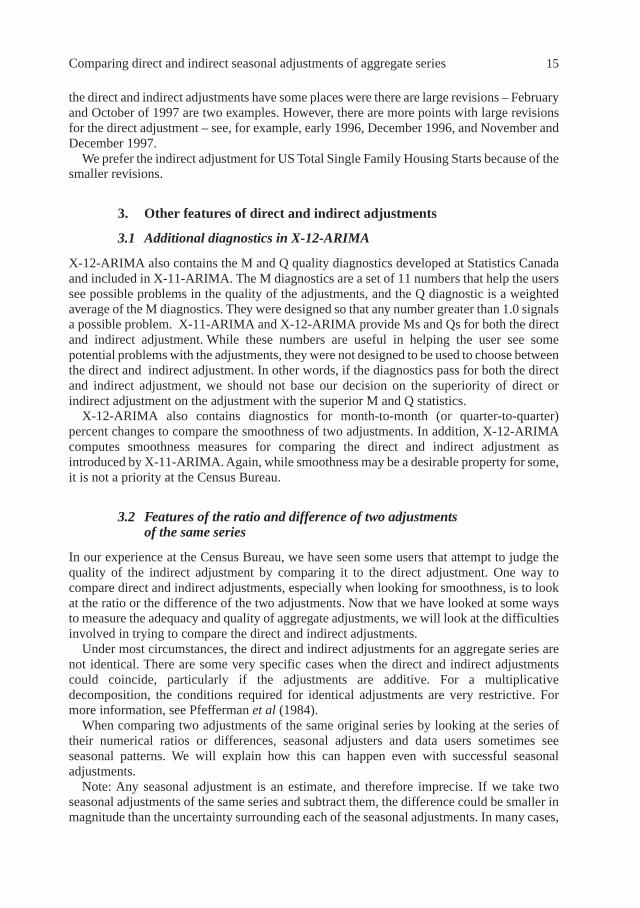
the direct and indirect adjustments have some places were there are large revisions – Februaryand October of 1997 are two examples. However, there are more points with large revisionsfor the direct adjustment – see, for example, early 1996, December 1996, and November andDecember 1997.
We prefer the indirect adjustment for US Total Single Family Housing Starts because of thesmaller revisions.
3. Other features of direct and indirect adjustments
3.1 Additional diagnostics in X-12-ARIMA
X-12-ARIMA also contains the M and Q quality diagnostics developed at Statistics Canadaand included in X-11-ARIMA. The M diagnostics are a set of 11 numbers that help the userssee possible problems in the quality of the adjustments, and the Q diagnostic is a weightedaverage of the M diagnostics. They were designed so that any number greater than 1.0 signalsa possible problem. X-11-ARIMA and X-12-ARIMA provide Ms and Qs for both the directand indirect adjustment. While these numbers are useful in helping the user see somepotential problems with the adjustments, they were not designed to be used to choose betweenthe direct and indirect adjustment. In other words, if the diagnostics pass for both the directand indirect adjustment, we should not base our decision on the superiority of direct orindirect adjustment on the adjustment with the superior M and Q statistics.
X-12-ARIMA also contains diagnostics for month-to-month (or quarter-to-quarter)percent changes to compare the smoothness of two adjustments. In addition, X-12-ARIMAcomputes smoothness measures for comparing the direct and indirect adjustment asintroduced by X-11-ARIMA. Again, while smoothness may be a desirable property for some,it is not a priority at the Census Bureau.
3.2 Features of the ratio and difference of two adjustmentsof the same series
In our experience at the Census Bureau, we have seen some users that attempt to judge thequality of the indirect adjustment by comparing it to the direct adjustment. One way tocompare direct and indirect adjustments, especially when looking for smoothness, is to lookat the ratio or the difference of the two adjustments. Now that we have looked at some waysto measure the adequacy and quality of aggregate adjustments, we will look at the difficultiesinvolved in trying to compare the direct and indirect adjustments.
Under most circumstances, the direct and indirect adjustments for an aggregate series arenot identical. There are some very specific cases when the direct and indirect adjustmentscould coincide, particularly if the adjustments are additive. For a multiplicativedecomposition, the conditions required for identical adjustments are very restrictive. Formore information, see Pfefferman et al (1984).
When comparing two adjustments of the same original series by looking at the series oftheir numerical ratios or differences, seasonal adjusters and data users sometimes seeseasonal patterns. We will explain how this can happen even with successful seasonaladjustments.
Note: Any seasonal adjustment is an estimate, and therefore imprecise. If we take twoseasonal adjustments of the same series and subtract them, the difference could be smaller inmagnitude than the uncertainty surrounding each of the seasonal adjustments. In many cases,

16 Hood and Findley
A(1)t =
Yt and A(2)
t = Y
t
St(1) St
(2)
At(1) – At
(2) = (Yt – St(1)) – (Yt – St
(2)) = St(2) – St
(1)
the differences between the two adjustments are smaller than the standard error of theirregular component, a natural measure of uncertainty.
To compare multiplicative adjustments, it is more natural to look at ratios instead ofdifferences. With series that are adjusted additively, it is more natural to look at differencesinstead of ratios.
3.2.2 Apparent seasonality in the ratios and differences
It is simple to show algebraically that residual seasonality in the ratio (and the difference ifthe adjustment is additive) of two adjustments of the same series can be a natural occurrenceand not necessarily an indication of a problem in either adjustment. If you have twoadjustments of the same series, and if the seasonal factors of both adjustments show very littleevolution over time, then the ratio of the two adjusted series will be seasonal.
We will focus on quarterly adjustments in the equations below because they are somewhatsimpler than the equations for monthly adjustment. Similar equations also hold for monthlyseries.
Let Yt be the original series. Let St(1) be one series of seasonal factor estimates. Let St(2) be asecond series of seasonal factor estimates.
For multiplicative adjustment, the adjusted series, At is the original series divided by theseasonal factor estimates. So from the two series of seasonal factors we have two differentadjustments:
If both seasonal factor estimates are periodic, i.e., St-4(1)
= St(1) and St-4
(2) = St
(2) for all t, then theratio will be periodic also, and we will see a seasonal pattern in the ratio since
(1)
Let’s look at a conceptual example. Suppose the seasonal factor for the first adjustment, St(1) is
1.07 for quarter one in the most recent year, telling us the original unadjusted quarter onenumbers should be decreased by 7%. Let’s also assume that the estimates of the seasonalfactors for quarter one are reasonably stable (St-4
(1) � St(1)), so that the estimates for the first
quarter of every year are approximately 1.07. Let’s say that the seasonal factor for the secondadjustment, St
(2), is 1.04 for quarter one in the most recent year and the estimates of theseasonal factors are stable. Therefore, when we divide both seasonal factors into the sameoriginal series, the ratio of the two seasonal factors (see equation (1) above) for every firstquarter is 1.04/1.07 = 0.972. If the same kind of stability is found in the quarterly estimates forquarters two, three, and four, then we have a series of ratios that are periodic, we will observea seasonal pattern in the ratio.
For additive adjustment, the basic principles are the same. The adjusted series, At is theoriginal series minus the seasonal factor estimates. To compare the two adjustments, wewould take differences instead of ratios.
If both seasonal factor estimates are periodic, then the difference of the seasonal factorswould also be periodic and therefore seasonal.
At(1)
= Yt / St
(1) =
St(2)
= St-4
(2) =
A(1)t-4
At(2)
= Yt / St
(2) =
St(1)
= St-4
(1) =
A(2)t-4

Comparing direct and indirect seasonal adjustments of aggregate series 17
3.3 Example – direct/indirect ratio for total exports
We will compare a default X-12-ARIMA run for the direct adjustment to the indirectadjustment for US Total Exports. We will show that we can find residual seasonality in theratio of the two adjustments. This finding does not suggest there is residual seasonality ineither the direct or the indirect adjustment.
We first point out that the range of the differences (and of the ratios) are very small inmagnitude compared to the original series. The differences are in the range of $1 or $2 billion,compared to the approximately $170 billion of Total Exports – on the order of 1% of TotalExports.
3.3.1 Indirect adjustment for total exports
We can look at the spectral diagnostics in X-12-ARIMA to see if there is evidence ofseasonality. The spectral graphs for the original (unadjusted) series and for the seasonallyadjusted series are shown below.
Note that the spectrum of the original series in Figure 7 has a somewhat broad peak at bothseasonal frequencies: ¼ cycle per year and ½ cycle per year. This is an indication of changingseasonality present in the original series. Notice that peaks at the seasonal frequencies aresuppressed by the seasonal adjustment as shown in Figure 8. Therefore, we can concludethere is no estimable seasonal effect still present in the seasonally adjusted series.
Figure 7: Spectrum of the original series, quarterly total exports
-30
-40
-50
-20
-10
-30
-40
-50
-20
-10Decibels
Seasonal frequencies
Frequencies1/4 1/2
Spectrum of the differenced logged original seriesTotal exports, summed to quarters

18 Hood and Findley
3.3.2 Direct adjustment for total exports
We can do a similar analysis of the direct adjustment for Total Exports. If we do a defaultX-12-ARIMA run for Total Exports, we see no sign of residual seasonality for the directadjustment as well.
3.3.3 Direct/indirect ratio
Figure 9 shows the ratio of the direct and indirect adjustment for Total Exports in a year overyear graph. We can see the indications of seasonality in the ratio. Generally, we see a firstquarter to second quarter increase, a third quarter to fourth quarter decrease, and a fourthquarter to first quarter increase.
-40
-50
-60
-30
-20
-40
-50
-60
-30
-20Decibels
Frequencies1/4 1/2
Seasonal frequencies
Figure 8: Total exports, spectrum of the seasonally adjusted series(Indirect adjustment)
1.008
1.006
1.004
1.002
1.000
0.998
0.996
0.994
0.992
0.990
1.008
1.006
1.004
1.002
1.000
0.998
0.996
0.994
0.992
0.990Q4 Q1Q3Q2Q1
19991998199719961995
Figure 9: Total exports, ratio between the direct and indirect adjustments

Comparing direct and indirect seasonal adjustments of aggregate series 19
The X-12-ARIMA diagnostics showed signs of estimable seasonality, among them, the Ftest for stable seasonality was large enough, at 33.1, to show possible seasonality present. Thespectral graph shown in Figure 10 also shows signs of moving seasonality in the ratio – broadpeaks at ¼ and ½.
4. Possible future SEATS adjustments for selected series
We are researching the use of SEATS adjustments for some series. We expect that in the nexttwo or three years, we might produce seasonal adjustments for some series from SEATS andfor the rest from X-12-ARIMA, giving us an indirect adjustment from the seasonaladjustment of choice.
4.1 Potential benefits
For some of our more irregular series, we can get smaller revisions with a SEATS adjustment.If the series is large enough in value, the improvement in the revisions can also be seen at theTotal Import or Total Export level. There are other series where the adjustments from X-12-ARIMA have better diagnostics.
We have also found that for a majority of series, the seasonal adjustments from SEATS andX-12-ARIMA are almost identical. For this reason also, we are not concerned with mixing theadjustments from the two programs for an indirect adjustment. We expect that the totals willbe very close even if we use SEATS for some series. We also intend to use SEATS only whenthere is a clear preference for the seasonal adjustment for SEATS.
Even with our expectations, we would still be very careful to investigate the diagnostics forthe monthly and quarterly totals no matter the program that produced the adjustment.
Figure 10: Spectral graph, ratio between the direct and indirect adjustments(Spectrum of the differenced original series – direct/indirect ratio using default direct adjustment)
-50
-60
-70
-80
-40
-30
-50
-60
-70
-80
-40
-30Decibels
Frequencies1/4 1/2
Seasonal frequencies

20 Hood and Findley
4.2 Potential problems
In several of our earlier studies at the Bureau (Hood and Findley 1999; Hood, Ashley, andFindley 2000; and Hood 2002) we found that SEATS needs more diagnostics before we canrecommend using SEATS for production work at the Bureau. We have been able to get X-12-ARIMA’s spectral graphs for individual series run in SEATS, or in aggregate series with someSEATS adjustments by running the final seasonally adjusted series back through X-12-ARIMA. However, it was very difficult to get revision information from SEATS.
At the Census Bureau, we have a test version of X-12-ARIMA that has access to the SEATSalgorithm. This allows computation of similar diagnostics for both programs to compareadjustments between the two programs, including revision diagnostics, and the ability tograph both adjustments in X-12-Graph.
Diagnostics for the SEATS adjustments are useful not only to make the comparisonbetween the two programs much easier; in addition, the diagnostics can point to problemswith the SEATS adjustment. For example, SEATS can induce residual seasonality into theseasonally adjusted series when the original series isn’t seasonal. It is also possible to haveunreasonably large revisions when TRAMO selects certain types of models. For moreinformation, please see Hood (2002).
Because of the potential problems with SEATS adjustments, we want to be very carefulbefore recommending a SEATS adjustment for a particular series.
5. Conclusions
Spectral and revision diagnostics for the aggregate adjustment can be very helpful indetermining the best level of aggregation for a particular set of series.
When two competing estimates of the seasonal factors of a time series are both ratherstable, in the sense that each calendar month’s (or calendar quarter’s) factor changes littlefrom one year to the next, then the factors from the two adjustments will differ in a consistentway. The presence of such a seasonal component does not, by itself, indicate inadequacy ineither of the adjustments.
No matter the seasonal adjustment software used, it is very important to be able to haveaccess to diagnostics. Though we see potential for SEATS adjustments at the Census Bureau,some care should be taken with SEATS adjustments. SEATS can induce seasonality into theseasonal adjustment of a nonseasonal series. The spectral diagnostics available in X-12-SEATS are very important to be able to see if the original series is seasonal or not and if thereexists residual seasonality in the seasonally adjusted series or the irregular component.
6. Acknowledgements
We are grateful to Brian Monsell for his software support with X-12-ARIMA and to KathyMcDonald-Johnson for her help with the research. We also thank Agustin Maravall for hisadvice and instruction on how to use TRAMO/SEATS, and Kathy, Brian, David Dickerson,Diane Oberg, William Bell, Michael Shimberg and Nash Monsour for comments on earlierversions of the paper.

Comparing direct and indirect seasonal adjustments of aggregate series 21
7. References
Dagum, E. B., (1979), On the Seasonal Adjustment of Economic Time Series Aggregates: ACase Study of the Unemployment Rate, Counting the Labor Force, National Commissionon Employment and Unemployment Statistics, Appendix, 2: 317-344.
Findley, D. F., D. E. K. Martin, and K. C. Wills, (2002), Generalizations of the Box-JenkinsAirline Model, to be published in the Proceedings of the Business and Economics Section,American Statistical Association: Alexandria, VA.
Findley, D. F., B. C. Monsell, W. R. Bell, M. C. Otto and B.-C. Chen, (1998), NewCapabilities and Methods of the X-12-ARIMA Seasonal Adjustment Program (withdiscussion), Journal of Business and Economic Statistics, 16: 127-176.
Findley, D. F., B. C. Monsell, H. B. Shulman, and M. G. Pugh, (1990), Sliding SpansDiagnostics for Seasonal and Related Adjustments, Journal of the American StatisticalAssociation, 85: 345-355.
Hood, C. C., (2001), X-12-Graph: A SAS/GRAPH® Program for X-12-ARIMA Output,User’s Guide for the X-12-Graph Interactive for PC/Windows, Version 1.2, Bureau of theCensus, U.S. Department of Commerce.
Hood, C. C., (2002), Comparison of Time Series Characteristics for Seasonal Adjustmentsfrom SEATS and X-12-ARIMA, to be published in the Proceedings of the Business andEconomics Section, American Statistical Association: Alexandria, VA.
Hood, C. C., J. D. Ashley, and D. F. Findley, (2000), An Empirical Evaluation of thePerformance of TRAMO/SEATS on Simulated Series, Proceedings of the Business andEconomics Section, American Statistical Association: Alexandria, VA.
Hood, C. C. and D. F. Findley, (1999), An Evaluation of TRAMO/SEATS and Comparisonwith X-12-ARIMA, Proceedings of the Business and Economics Section, AmericanStatistical Association: Alexandria, VA.
Pfefferman, D., E. Salama, and S. Ben-Turvia, (1984), On the Aggregation of Series: A NewLook at an Old Problem, Working paper, Bureau of Statistics, Jerusalem, Israel.
U.S. Census Bureau, (2002), X-12-ARIMA Reference Manual, Final Version 0.2, Washington,DC: U.S. Census Bureau.

22 Hood and Findley

2
A class of diagnostics in the ARIMA-model-based decompositionof a time series
Agustín Maravall
�� ����������
������������������� ������������������������������������������������������������������������������������� ������������!��""#������$���%&'(�$'������)*��+���������,����""-�!�$�������������.����������������������� �/��,�����,�����������������������/��������,��,��.�������.�!�$���%&'(�$'����.���������������������������0��������1�������/���������������������������1��������"#2��3�����������$������"#������������!%,��� ��� ������ ����� ��� ��/���������� ��� ���������� ���� ��� ���.�����/�� ���� 4������
�����������/�/5��������0��������������0����������� �6�������0��7�/�������������/���������������������/�/����������.�����������������0��,�!�1����������������/������������������.�������������������������0�����������/������������0�������������.����������/���������/���������/���������,����������/�������������������.���� �������������������������/��������0��������������������.�/��� ��5��������������������������0������,������!��'�����������/����� ���� ��5� ���� 1���� �""8�� 1���� ���� 3������� �"#9�� 1�:� ;���/�� ���� <� 0���� �"#=�1�����.������>�������"#8��"#9��?��,����������;���/���"#���?��,����������$�����"=-�3��������"#8������,�����"#=��""8������,��������;�������"""��;���/���"#2��"="��$�������3��������"=#!������������������/����������������,�����������������������0����������������������������
�����'4�����(����������'(����������������������0���,���/���������!�@�� ���.��������������������0�����������,��������������������������������������0���,��������������,�������� ����������������������/������������������ ������.��,����������������/���0���0�������������� �/� ���� /������� �������� �������� ���.�����/�!�A��� ��� ������������ ���,����� 0�� ��� � �������/����������0������������!�>������������,�������4���������������������������������/��������������������������������0������0��B�������������/�����������.��������.����B�C����'(�$'����.�����/�����,�������/���/���������������������������������������������,�����/���� ��� ��������� /��������� ��� �.�������� ��� ��� �������/��� ,�����/�� ��� ��� ��'(����������B�������������������/�������������������������.�������� ����������������0�������������������B�����������/�����,��������������.������ ��������������������/�����0�B�D�� ��� ��� ���� ��� ��� ������������ .�,��� 0�� ��� � �� ������/��� /��� 0�� ����� ��/������������!���������1�������/������������������������������5��������������������� ��5������������������������/����������/���0������������������.���������,������/���/�����!
�� �������������������������������������
'����������0�/5� ����������������������.���/������������������������..��.���������,����"#=�� ��� ��������� �E�.��� �"#2�� 4������� ����������� /�/5� ����F� 6���� ��/����/���������������������.�����/��������7!�����5���������F�>��������������/B�3� ���/������ ����� 0�B� ������ ���� ���������� ������� ������ ���������.������ ��� �������������/����������!�>�������������/�����������������/B�>���������.�����/������� �����������.� �� ��� ���� 5�� � � � ��/� ����/����������� ������ 0�� �������� ��� ��� ����.����

24 Maravall
���������� �����������5���������.����� �����������������/����������!��������������G�����������������/�/5�� �/�/���/���������0����������0�����������������/�������!�$��������5�����/���/����+��� ����� ����� ���.�����/� /�/5�� ��/� ��� ���� �:������ ��� 6������.� �����7���.�����/��� ������������!��""2�!$����4������������������/�/5��/��������0����������������������/�������������������������
�0������� ��� ���������������0��������/���������'(�$'� ����� ��� ��/�� ��5� ���0���.���������������������H'�1������������?�����������������/����!��1�������������������������������� �����/������ ���� ����.��� ����� ����������.� ����� /�/5�� ����� ��������/��� ������ 0�������������������0���������/����!�$������������/��������������0�����������������������/��0�� ����,��� ���� ���� �:������ ��� ��� �����0��� ��� ����� ��� �������/��� ����/����������� ���� ������.�������������������� �/����4�������F�6� ���/������������B7�/���0����� ����!
�� ������������������������������������� ������!
��������������,����0��� tx ������ ����������������
tt a)B(x)B()B( θ=δφ ���
���� ��� ��� �� ���������� � !�!�� ,����0��� ��!�!� �� ���� )V,0( a � ,����0���� )B(φ � �������� �������������������.�����,������������������ ��� ���0�/5 �������������1� )B(δ �������� ����������������� ����������� /��������.� ��� ����� ������ ���� ��������/��� ��/� ��� ���� �:�����
12)B( ∇∇=δ ������ )B(θ ���������,����0�����,��.��,���.���������������������1������1�:����
I��5�����"=2�!�$�����������+�������������� 1Va = !J���:��0������������� ����/�������������0���,���/�����������H?�
ttt nsx += ���
������������:������:��K��'��������?���������L�'��������������������'���������!�� �����.��������������������������������������.���.�������� ts ���� tn ��//�����.�������������/��������4���/�� )B(δ ����� )B(φ �/���0����/����+�����
)B()B()B( ns δδ=δ
)B()B()B( ns φφ=φ
� ����:��������� S)B( 212 ∇=∇∇=δ � ����'�K���L�1�L�1��L�!!!�L�1���/�������������������
��������������� S)B(s =δ �� .))B( 2n ∇=δ ��������������H?���������,������'(�$'�����������
�������F
ststss a)B(s)B()B( θ=δφ �M�
ntntnn a)B(n)B()B( θ=δφ �9�
�������������������������������/����������H?�����,������� ���+�������������,�����/���4�������D������D�������/��,���!�$���������������������1������1����� ����������,�����/��D������D���������������������������������
ntssnstnnst a)B()B()B(a)B()B()B(a)B( δφθ+δφθ=θ

A class of diagnostics in the ARIMA-model-based decomposition of a time series 25
��.����� ��� ����� ����������� ������������ ����� ����,���� �""8�!� $�� ���,����� ���������������� /��������/�� 0�� ���� ��� ������ ���� ��� �0���,��� ������� ���� ��� ����� ���� ��/����������� ��� ����� ��� ��� ���/������� ��� ,����� ���� ���� �������0��� ��/��������������������������������������/�����������������!(:�����������M�������9�����,�������������������������/���/���������!�$����/���������
������,����0���,������� ����0������������0���������'(�����������!� ������/��������������������.������0�����������������+����������������������.�,���0�
x)F,B(s tst ν= � )BF( 1−=
���� )F,B(sν �������>������@����.���,��>@��������!���������0���/������������������/���0��0�����������
tss
ss x)F()B(
)F()B(V)F,B(
ψψψψ=ν
���� )B(
)B()B(
.
.. φ
θ=ψ !������/��.�:��0�� ta)B(ψ �������/��/�������������������������0������F
tnns
s
ssts a
)F(
)F()F()F(
)B(
)B(Vs)B(
θ
φδθφθ=δ �8�
�����������������������!!�!����������������������������������������/����������������!!�!�����������/��,��.�������1�������� �� �/�/���0����������0������!�>�����.����/����/�����
tsts a)B(s)B( η=δ �-�
���� ta �������0�������������,�������������0���,��������������1���������������������+�������� ���/���� ���� ���� ,�����/�� ���� ����/������������ /��� 0�� /�������!� ��� ���� ��� ��,�����/����������/��������������������������/������'(����������������0������!�$��� ����0�������������������,�����/����������/�������������������������/���/���������.�,���0���M�!�������������������1�������/��'(�$'�� ��5�� �������������/�������0������������
������������������������������������������������������� ��/���������������������.!�����������/��/���������������� tn n)B(δ !�1�/5���� ����:����������.�,����������.�F�6$�����/�����/�������������� �������.����
/��������7� ������� ��� ����.����� /��������� ��� ��� !�!� �2D��!� J�����.� ��� 0�/���� tu
�:����������8��������������������������� tu �����������?����������� ��/�������? ������������
*tt a)B()B(y)B( δφ=θ �=�
���� *ta ������ !�!��2�D���,����0��!���������=��������6��,����������7�������������!��3��/�
�,��.�������������� tx � ��5�� �����? �����������.�����/������������������!�������� ���,�����������������������������������������������/���������������/�����
���/������ ��/� ���$���%� ��� �,����0��!�>�� ��/���� ���� ��� ���� ��� 6����/7� ��:��� ����������������>@������������/������ �����������
����:��K����N�!91�����N�!-1��� �#�

26 Maravall
��������������!��$������������������.����������������������1�:�I��5�����"=2!��?��,������$�����"=-���� ���������������������������������������������������������������������/�����������!�1������������������������������������������������������ ���/�����0�����6����������7������������/����,������������/���������0���������������!?��������������� ��� �������� ������� ��� �����99���������0���,������� �� ���5���� ��
�/������������������������.���������/���������������������������������/����������
32.)u(ˆ t1 =ρ
��,��.��������������,������0�����������������������������������/��!�����!M��6������/��?7B$����1���� �����������.���� ���!� ����������#������? ����O��������������������F
*t
12t
12 a)B1()B1(y)B6.1()B4.1( −−=−−
�����������������/����������O����
30.)u( t1 −=ρ !
$��������/��������������/���,������� 1ρ �K�!M������ 1ρ �K��!M2������/��,��������������0��� ������ ���������� ��� ������/�!� ����1�������P�� �����:�������� ����� 1�:� ���� I��5���� �"=��;����������"#��
�ρk )ˆ(V
��[ ]∑
−=−−+ ρρρ−ρρ+ρρ+ρ
m
mjkjjk
2j
2kkjkj
2j 42
T
1&
���������P������������ tu ��������������������!!�!�����������������������/����? ���� tu ������������������/��������������/����� 0j ≈ρ � mjfor > ! ��������:�������������0�����������'E�� 1ρ ��K�!2=9�������"8Q�?�������/�������,���������
1ρ ��4�������R ±ρ1ˆ ���'E�� 1ρ ��S����������������,���R!�=�!9=�S!�?������� 1ρ �K��!M2����������������������,��� ���� ��/�� �� /��� /��/����� 6����� ��� ���� ��/� �������,��� �?� ��� ��� ����.����/��������7!$�������//����0����������,������/���������������������.�����/���������/�����0��������
������/���/������������������/�/���/��������!������/����������������������2�������2��������
���������������/��������0���0�����!�$������.���������/������������0�/���� 83.)u( t1 −=ρ ����82.)u(ˆ t1 −=ρ � ��� 04.)ˆ(SD 1 =ρ !� $�� ,����� 84.1 −=ρ � �� � ����� /�������0��� ��� ��� "8Q
/�������/�������,���R�!=9���!"2�S!
�� ����� �������"����������������
���������,������:����������������/������ ����
��K��!#M� �/������������� tu �������������
����/������������������-��������������������������4���/�������� ���6�.��7�������������������.�����/��������!>��������1����������������������/��6�����������/�������������������.�������� �������
�����7!�$���������0���/����������/���/����������!�%��/���������������������������/���0�����.��������0��������������������������.�����/��������������/��������������������������/��������� ����� ���,���� �� .���� �:������ ��� ��� �.��� ��������� /���������!� $�������4���������������������� ������������������/���0��������� ��� ���� �����/�F� ����/��� ����:���������/�������������.��������������������/�������������/����������!
K��������
A class of diagnostics in the ARIMA-model-based decomposition of a time series 27
#� �����������������������������������������������
$�� ���,����� �:������ ���,����� �� ����� ���� ��� ������������ ����/����������� ��� ��� ����.����/�����������������!�$�������� ���0�����������������0����������������������������������������������������!(:������������������.���� ���!� ����:������ ��/���/������� )u( t12ρ � ��� )u(ˆ t12ρ ���������
3��F��T���K��������������:������ ��� 12ρ ������.����/���������.������������/��/��������F�6�������������/�����������������������.����7!�$�������/��������0���:���������������/�����������/� ��� ���� �:������ ��� '�� ������� ����� tn �!� ���� ��� ������ ���� tn
STt n)B(n δ= � �
����,�� )n( STt12ρ !� ��������/�������������� ��/����������������/�������/����������� )n(ˆ ST
t12ρ !H���.� 1�������P�� �����:��������� �� �0����� 'E� � 12ρ �!� �.���� �� /��� ����� ���3��F��T���K������������ 12ρ ������.����/���������.������� 12ρ �/��/��������F�6��������������/�������������/�����������������'��������7!>��/�����������5���������.������������!� ����:����������������������&�,����������������
����������������������&�,��������������!��.�,������������������//������/�������������/�,����������������������������/����������
���������,��������!�$��� ���������� ������ �������������������4������.�������5�����������������/�������������������������'������������������ ���������������� � ���/��������������������������/���������������������������!�$������ ���.�������/�������������:�����������������������
t12
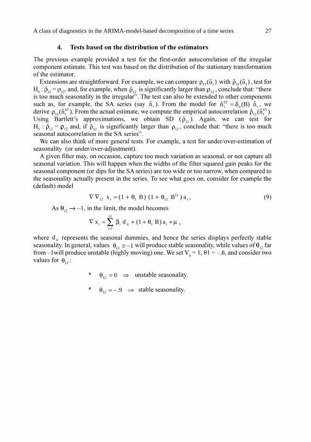
121t12 a)B1()B1(x θ+θ+=∇∇ �"�
���������N�����������������������0�/����
a)B1(dx t1
11
1iitit µ+θ++β=∇ ∑
=
���� itd � ����������� ��������������������������/��������������������������/�������0�������������!����.�������,������ 112 −≅θ � ���������/�����0��������������� ����,���������������������N� ���������/�������0�����.�����,��.�����!�>������D�K������K�N!-�����/��������� �,���������� 12θ F
U ⇒=θ 012 ��������0��������������!
U ⇒−=θ 9.12 �����0��������������!

28 Maravall
?����������������� �����/�����,����/��������������/����� ����������������������5�!
Figure 1: Series with stable and unstable seasonal
E������0�� )F,B(ν ������:��������/���������������������������������/�������������'��������!�'��������:������ )F,B(ν �K����������������������������� �/� ��������������
∑=
+ν+ν=νk
1j
jjj0 )FB()F,B(
$�� �������$���������� !$!������������������/����������������.�����4������
∑=
ων+ν=ωk
1jj0 )j(cos2)(G
���������������4���/��������������������������2�������������4������.�������������������.�,���0�
')�����K�R)����S�
J���.������������������/�������������������/������������,����0�����! �����T��K�,��1� ��:�������0�����
)(g)(SG)(g xss ωω=ω ��2�
J�5� �����������'�������������
)(g)(SG)(g xnn ωω=ω ! ����
$�� ���/������ )(gand)(g ns ωω ���� ��� ���/���� ��� ��� ����������� ��� ��� ��������/�������������'��������!�>��/���/��������������������/�����������������!
unstablestable
0 π

A class of diagnostics in the ARIMA-model-based decomposition of a time series 29
���H����0����������������������������������
Figure 2b: Underestimation of seasonality: SA series
Figure 2a: Underestimation of seasonality: seasonal component
�����������������������,����/���0�����5�����������.0�������������������������4���/������ �����N�������� 5 �����������N�������'��������!
x11 seas. comp.series
0 π
x11 SA seriesseries
0 π

30 Maravall
0��'��0��������������������,������������
Figure 3a: Overestimation of seasonality: seasonal component
Figure 3b: Overestimation of seasonality: SA series
3���������/���������'�������������/����������� ���!H���.�������� ���������'(�$'�0�������������� �/�/����������������������������������
����������������������������������������������������� �����>@�������� )F,B(sν �������������������/��������/����/�����/�����������������!�$�� !$!���� )F,B(sν ������)���F
)(g/)(g)(G xss ωω=ω
�������0������������/������������������������������������/�������������'�������������.�,��0����2����������!�?�������.������� �����/��������������������������F
x11 seas. comp.series
0 π
x11 SA seriesseries
0 π

A class of diagnostics in the ARIMA-model-based decomposition of a time series 31
���H����0���������������/�����'(�$'�
Figure 4a: Unstable seasonality: SEATS seasonal component
��� ��� ����� ���� ��� ���.�� ���5�� ��� ��� ���.0������� ��� ��� ��������� ���4���/���� �,������������!
Figure 4b: Unstable seasonality: SEATS SA series
SEATS seas. comp.series
0 π
SEATS SA series estimatorseriesSEATS SA series
0 π

32 Maravall
$�����������������������������/���������������������������� �������������/���������������'�������������������������������� ����������������������5������������������/����!
0��'��0���������������/�����'(�$'�
Figure 5a: Stable seasonality: SEATS seasonal component
SEATS seas. comp.series
0 π
SEATS SA series estimatorseriesSEATS SA series
0 π
Figure 5b: Stable seasonality: SEATS SA series

A class of diagnostics in the ARIMA-model-based decomposition of a time series 33
����� ���������$�������%������
��� ��/�������������/���������������������������'������������������,������ ���:������������������ ������������������������������������������:/����,�����/��������'��������� ����,��������������������������������������������,�����/��������'���������������������!
Figure 6a: Unstable seasonality: estimator of the SA series
Figure 5b: Stable seasonal: estimator of the SA series
SEATSX11
0 π
SEATS X11
0 π

34 Maravall
$���:���������������������.���������/������ �����������������������������������������,���� ���0��� ��� ������� ���/����/� ,��������� ��� ������� ���� �,��������� �����,�� ���� ��/,���������������������!�%�����/�������� �����������������������0��������������������������.��� ���/����/� ��������� ,��������� ��� ������� ���� ������������ ����� ����,�� ���� ��������,���������!��������� �������������������������������������������������������������/��������,�����/�� �����,�������������� ���������,���������������� ��� ���������/���������,�����/��������������������������������&�,�������������������/���������,�����/�!;��/�����.����0������������������8��������������������T�� ��5�� �����������/���,�������
���,�����/����������������������������������������/�������������������D��!�>��/��������.���1�������P�������:�����������/���������������������,��������������,�����/�����������
2
1
m
1j
2jss 21
T
2V)V(SD
ρ+= ∑
=�
���� jρ ������������/��������������������0���������8�!�$��� ��/������������ ��������3��F�DT�K�D�����/����������!���������:������'��K����������/������������� ���,���0������
�D��K�!2-= DT���K�!�22 �'E�K�!2�2�
�� �����/��/�����������������6�,����/������,���������������������������7!%��� /��� ���5� ��� ����� �:��������!���� ���������� ���� ��� ��� ����� ��.!������.� ��
�������/��� /���������� ���� ��/���������� ��� ��� ���� 5�� �� ����� <����,�� )������ ���?��,�����"="�� ������'(������������ ���� ����/�� �����/����/�����������0�� ���� ���! ���� ������ �8�� ���� ��� �4��,������ �:��������� ���� �T� �� �� /��� �0����� ��� �������/��/����/�,�����/������/����/��������������/����������������������������������)*��+�����,����22��!� ���������1�������P�������:���������/��������0���:�������������������������������/�����������!�$�����������0������ ��/��������:������0�����������������������F�6$������������/�/�����������0�� ������������������������.���������������7!�����������:���������������,����0������������������������.����������.�����/����/��������
�����������������������������������������/����.����������� ����������0�������������!�$�������������������������������������6�������0��7�������.��������������,������,��������.��0��������������������������5��������,������������������������������������������������� ������������������0�����!�>�������,���������������.�����������������/�����������5���������������������������������.���6�������0��7!���� ������4���/������������0���������������������8Q���������������������0����������!$���/�/5�/��������0����������������������/�������������'(�$'������64������7����.�����/�
��� ��� ������ ��� �,��.� �� 6��/�7� ��������!� 1��� .�,��� ���� ��� ,��������� /���������� ��� �����.�����/��������������������,�����������������������������������������1�������/��������.�,�������������/�����/������������:����������������������,�����""#�
kss[ t|tt >− S
���� �T�� K� ������ ���������� ���� �T�����K� /��/������� ���������� ��� �T�� �0������� ��� ��� �������������.� ���:�!�$��������������,�����������0�0�������������,��������������/��/������������������������/���������������������������.�,��������������.�������������������,���5!J�����.����������������,������������/��/����������������
���K��T��N�T����
��������� ������� ��� ��������0������� �;���/���"#2������ ������0�0������ )kd(P t > � /���0�/�������!� $��� ���0�0������ ����� 0�� ��� �������/��� ,����� ����/������ ��� ��� �������
;��0 �
�����

A class of diagnostics in the ARIMA-model-based decomposition of a time series 35
���������!�)�,���5�;�����V�5������������.���������������������������������������������0���,���������!� ���������������������0�0������ ����0�����.����,����0�,��!�8��������������������� ����0�������!�1���������������������������'(�������������������/����������������������0�0����������/��������0�,����5������������/�����,�����!�$������ ������/��� ��� ��� ,�����/�� ���� ����&/�����/������������ ��� ��� ����������� /���������� ��� ���6�������/��7� ,����� ��� ��� ���4���/�� ����/���� ��� ��� ������� /��� ���,���� ��� ��1���.�����/!�J��.����������/���0�� ������������������4���/������������0�0��������������0���������������������������������.����������.�����/�������������� ����������������������.�!�'���������5������ �����0��������.���F�6�T�����������/��0�/����������,�����������7� ������������������������������1�������/� ��������F�6$�����������/�����������������.������� ������������/�����,���������������/��/����������������7���.���������/���/����������������!1��� ��� ����� ���� ��� ��1� �������� ���,���� ����,���� ���� ���������� ������������ ���/������������/�����!�3� �,��� ������0������.�����/��������������/���0��������������������� �����4����� ���������� ��� ��� ��/�� ���� ���������� ��� ����0���������� ��� �����1������/������������������������5����������������� �/�����������������������0���������/�����!
References
Bell, W. R., (1995), Seasonal Adjustment to Facilitate Forecasting. Arguments for NotRevising Seasonally Adjusted Data, Proceedings of the American Statistical Association,Business and Economics Statistics Section.
Bell, W. R. and Hillmer, S. C., (1984), Issues involved with the Seasonal Adjustment ofEconomic Time Series. Journal of Business and Economic Statistics 2, 291-320.
Box, G. E. P. and Jenkins, G. M., (1970), Time Series Analysis: Forecasting and Control,San Francisco: Holden-Day.
Box, G. E. P., Pierce, D. A. and Newbold, P., (1987), Estimating Trend and Growth Rates inSeasonal Time Series, Journal of the American Statistical Association 82, 276-282.
Burman, J. P., (1980), Seasonal Adjustment by Signal Extraction, Journal of the RoyalStatistical Society A, 143, 321-337.
Burridge, P. and Wallis, K. F., (1985), Calculating the Variance of Seasonally AdjustedSeries”, Journal of the American Statistical Association 80, 541-552.
Burridge, P. and Wallis, K. F., (1984), Unobserved Components Models for SeasonalAdjustment Filters, Journal of Business and Economic Statistics 2, 350-359.
Cleveland, W. P. and Pierce, D. A., (1981), Seasonal Adjustment Methods for the MonetaryAggregates, Federal Reserve Bulletin, Board of Governors of the Federal Reserve System,December 1981, 875-887.
Cleveland, W. P. and Tiao, G. C., (1976), Decomposition of Seasonal Time Series: A Modelfor the X-11 Program, Journal of the American Statistical Association 71, 581-587.
Dagum, E. B., (1980), The X11 ARIMA Seasonal Adjustment Method, Statistics Canada,Catalogue 12-564e.
Findley, D. F., Monsell, B. C., Bell, W. R., Otto, M. C. and Chen, B. C., (1998), NewCapabilities and Methods of the X12 ARIMA Seasonal Adjustment Program (WithDiscussion), Journal of Business and Economic Statistics, 12, 127-177.
Findley, D. F., Monsell, B. C., Schulman, H. B. and Pugh, M. G., (1990), Sliding-SpansDiagnostics for Seasonal and Related Adjustments, Journal of the American StatisticalAssociation, 85, 410, 345-355.
Gómez, V. and Maravall, A., (2001), Seasonal Adjustment and Signal Extraction in EconomicTime Series, Ch. 8 in Peña D., Tiao G. C. and Tsay, R. S. (eds.) A Course in Time SeriesAnalysis, New York: Wiley.

36 Maravall
Gómez, V. and Maravall, A., (1996), Programs TRAMO and SEATS. Instructions for theUser, (with some updates). Working Paper 9628, Servicio de Estudios, Banco de España.
Hillmer, S. C., (1985), Measures of Variability for Model-Based Seasonal AdjustmentProcedures, Journal of Business and Economic Statistics 3, 60-68.
Hillmer, S. C. and Tiao, G. C., (1982), An ARIMA-Model Based Approach to SeasonalAdjustment”, Journal of the American Statistical Association 77, 63-70.
Maravall, A., (1998), Comments on the Seasonal Adjustment Program X12ARIMA, Journalof Business and Economic Statistics, 16, 155-160.
Maravall, A., (1995), Unobserved Components in Economic Time Series, in Pesaran, H. andWickens, M. (eds.), The Handbook of Applied Econometrics, vol. 1, Oxford: BasilBlackwell.
Maravall, A., (1987), On Minimum Mean Squared Error Estimation of the Noise inUnobserved Component Models, Journal of Business and Economic Statistics 5, 115-120.
Maravall, A. and Planas, C., (1999), Estimation Error and the Specification of UnobservedComponent Models, Journal of Econometrics, 92, 325-353.
Nerlove, M., Grether, D. M. and Carvalho, J. L., (1979), Analysis of Economic Time Series: ASynthesis, New York: Academic Press.
Pierce, D. A., (1980), Data Revisions In Moving Average Seasonal Adjustment Procedures,Journal of Econometrics 14, 95-114.
Pierce, D. A., (1979), Signal Extraction Error in Non Stationary Time Series, Annals ofStatistics 7, 1.303-1.320.
Priestley, M. B., (1981), Spectral Analysis and Time Series, London: Academic Press.Tiao, G. C. and Hillmer, S. C., (1978), Some Consideration of Decomposition of a Time
Series, Biometrika 65, 497-502.

3
Seasonal adjustment of European aggregates: direct versusindirect approach
Dominique Ladiray and Gian Luigi Mazzi
1 Introduction
Most of the European and Eurozone economic short term indicators are computed eitherthrough “horizontal” aggregation, e.g. by country, or through “vertical” aggregation, e.g. bysector or product. Three main strategies can be used to obtain seasonally adjusted figures:• The direct approach: the European indicator is first computed by aggregation of the raw
data and then seasonally adjusted;• The indirect approach: the raw data (for example the data by country) are first seasonally
adjusted, all of them with the same method and software, and the European seasonallyadjusted series is then derived as the aggregation of the seasonally adjusted national series;
• The “mixed” indirect approach: each Member State seasonally adjusts its series, with itsown method and strategy, and the European seasonally adjusted series is then derived asthe aggregation of the adjusted national series.Unfortunately, these strategies could produce quite different results. The choice between
the first two approaches has been the subject of articles and discussions for decades and thereis still no consensus on the best method to use. On the contrary, some agreement appears inthe literature on the fact that the decision has to be made case by case following someempirical rules and criteria (Dagum [2], European Central Bank [3], Lothian and Morry [12],Pfefferman et al. [13], Planas and Campolongo [14], Scott and Zadrozny [15] etc.). The lastapproach is often used and, as it cannot be derived from a simple adjustment, is rarelycompared to the others.
The choice between the methods cannot be based on accuracy and statistical considerationsonly. To publish timely estimates, Eurostat must often work with an incomplete set of nationaldata. The indirect approaches imply estimation of missing raw and seasonally adjusted dataand therefore different models have to be estimated, checked and updated. The directapproach is obviously easier to implement and would be preferred except if there is a strongevidence that an indirect approach is better.
Section 2 of the paper is devoted to a detailed presentation of the direct vs indirect problem,its implications and some non statistical guidelines for the choice of a strategy. Section 3presents the various quality measures that can be used to make the right choice and themethodology used in the applications. Both of the applications presented in this paperconcern the Quarterly National Accounts: the geographical aggregation problem in Section 4and the sectoral aggregation problem in Section 5. TRAMO-SEATS and X-12-ARIMA wereused for these applications; the same quality measures have been computed for both seasonaladjustment programs and, when possible, the mixed indirect approach has been compared tothe other approaches.

38 Ladiray and Mazzi
2 The direct versus indirect problem
Nowadays it is common to decompose an observed time series Xt into several components,themselves unobserved, according to, for example, an additive model:
Xt = TCt + St + Dt + Et + It (1)
where TCt, St, Dt, Et and It designate, respectively, the trend-cycle, the seasonality, the trading-day, the Easter effect and the irregular components.
The seasonality St and the calendar component (Dt + Et) are removed from the observedtime series to obtain the seasonally adjusted series At = TCt + It.We will suppose from now on that Xt is an European indicator computed by linear aggregationof N national indicators (N = 15 for the European Union or N = 12 for the Eurozone); in thisaggregation, each Member State n has a weight ωn. Therefore we have:
Xn,t = TCn,t + Sn,t + Dn,t + En,t + In,t (2)
and: Xt =N∑
n=1
ωnXn,t
Note that the weights can be positive and sum up to 1, as in the IPI case, or can be all equalto 1, as in the GDP case.
2.1 Direct, indirect and mixed indirect seasonal adjustments
The seasonally adjusted series At of the European aggregate Xt can be derived from at leastthree different strategies:• The direct approach consists in adjusting directly the aggregate. The direct seasonally
adjusted series is noted AtD;
• In the indirect approach, all the national indicators Xn,t are seasonally adjusted, with thesame method and software, and the European seasonally adjusted series is then derived asthe aggregation of the seasonally adjusted national series. Thus we have:
AIt =
N∑
n=1
ωnAn,t
• In the “‘mixed” indirect approach: each Member State seasonally adjusts its series, with itsown method and strategy, and the European seasonally adjusted series is then derived asthe aggregation of the adjusted national series. The mixed indirect seasonally adjustedseries is noted At
M.The multivariate approach, which permits to derive simultaneously the seasonally adjusted
series for the aggregate and the components, must be mentioned at this stage as an alternative.This method has been proposed for many years (Geweke [6]) but given its computationalcomplexity, the limitations of existing programs and its lack of optimality with respect torevision errors, it is rarely used in practice and the univariate approaches are generallypreferred.

Seasonal adjustment of European aggregates: direct versus indirect approach 39
The mixed indirect approach is a quite popular strategy but, as it does not result from asimple seasonal adjustment process, it is scarcely studied by itself. The national seasonaladjustment policies can substantially differ for several reasons:• The methods are often different: some countries use a model-based approach (TRAMO-
SEATS, STAMP), other countries a non parametric approach (X-11 family);• The software, or the release, that implements the method can also differ: X-11, X-11-
ARIMA and X-12-ARIMA are currently in use in the European countries, sometimes inthe same institute;
• The revision policies can vary and Member States may use current or concurrent seasonaladjustments;
• Member States can perform themselves direct or indirect seasonal adjustments;• The strategy for the correction of calendar effects is usually not the same, the seasonal
adjustments are not performed on the same time span, the treatment of outliers can differetc.All these differences show how it is difficult to compare, from the theoretical point of view,
the mixed indirect seasonal adjustment to the direct and indirect ones. Furthermore, thesethree strategies are not the only possible ones and we can imagine for example a mixedapproach: a subset of the basic series can be first aggregated in one new component, thiscomponent and the remaining sub-series can then be adjusted and the adjusted aggregatederived by implication. In fact this procedure is frequently used since many of what areconsidered the basic components are themselves aggregates of other components, althoughthe latter are not always observed separately (Pfefferman [13]).
2.2 Could direct and indirect approaches coincide?
As far as the aggregate is a linear combination of the components and the seasonal adjustmentis a non-linear process, the answer is generally no, except under some very restrictiveconditions (see for example Pfefferman [13]). Thus, if the aggregate is an algebraic sum(GDP for example), if the decomposition model is purely additive (equation 1), if there is nooutlier in the series and if the global filter used in the seasonal adjustment process is the samefor all series, the two approaches are equivalent. If the decomposition model is multiplicative,it could be shown that the equivalence of the two approaches requires for instance that thereis no irregular, that the sub-series have identical seasonality patterns (or that the sub-serieshave identical or proportional trend-cycles) and that the lter used is the same for all sub-series. On the other hand, if the aggregate is a rate, any seasonal adjustment strategy thatproduces unbiased estimates will give different results (Dagum [2]).Clearly the reality is much more complex:• For the majority of economic series the additive model is not the most appropriate and the
series are adjusted using the multiplicative option. Such series may be converted to anadditive model by a logarithmic transformation, as in TRAMO-SEATS, but this will notensure the equivalence since the logarithm of a sum is not the sum of the logarithms.
• Outliers are frequently present in economic time series as the result of structural changes,anomalous conditions, external shocks etc.
• For model-based approaches, such as TRAMO-SEATS, the filter used for the seasonaladjustment is optimally derived from the characteristics of the series. It means that adifferent filter is associated to each series. In that case, direct and indirect adjustmentswould never coincide.

40 Ladiray and Mazzi
On the other hand, it may occur that sub-series are not very noisy, show a very similar trend-cycle or seasonal pattern and are affected more or less by the same external shocks. In theseconditions, the direct and indirect approaches could not be too different. These considerationsadvocate for measures of the differences between the various adjusted series; such indicatorswill be presented in section 3.2.
2.3 A priori advantages and drawbacks
The choice between direct, indirect and mixed indirect adjustment can be guided by somestatistical or non statistical considerations or by some a priori desirable properties.
1. The additivity constraint and the indirect approachesSometimes the additivity constraint plays an important role in some domains (quarterlynational accounts, balance of payments) or has to be assured as the consequence of a legalact (external trade). Then the indirect or the mixed indirect approaches appear to be therelevant ones. Furthermore, the mixed indirect approach seems to imply there is nodiscrepancy between national figures and European data. Nevertheless, some points mustbe precised:• Even with a direct approach it is always possible to assure ex post the additivity
constraint by distributing the discrepancies. Various univariate or multivariate statisticaltechniques exist to compute these adjustment factors.
• The additivity constraint is veriefied on the levels of the series. But users are moregenerally concerned with growth rates. Of course, as we have:
AIt+1 − AI
t
AIt
=1
∑Nn=1 ωnAn,t
N∑
n=1
(ωnAn,t × An,t+1 − An,t
An,t
)
the indirect growth rate is a weighted average of the sub-series growth rates, withweights that sum up to 1. Therefore, the indirect growth rate is always between thesmaller and the larger sub-series growth rate and in that sense, the indirect approach isconsistent. But you can have a majority of sub-series increasing while the global growthrate decreases: see some examples in Section 4.
• The additivity constraint has nothing to do with either the time consistency problem,requiring for example that quarterly and annual figures have to be coherent, or theconsistency between raw and adjusted data annual totals.
2. Some “statistical” considerationsMost of the statisticians involved in seasonal adjustment agree on one point: if the sub-components do not have similar characteristics or if the relative importance of the sub-series (in terms of weight) is changing very fast, indirect adjustment should be preferred.From the opposite point of view (Dagum [2]), if the sub-series have a similar seasonalpattern and more or less the same timing in their peaks and troughs, the direct approachshould be preferred. The aggregation will produce a smoother series with no loss ofinformation on the seasonal pattern.On one hand, as some studies show a synchronization of the cycles in the European Union(see for example Blake et al. [1]), the direct approach should be preferred. On the otherhand, some countries have strong specificities and this point is of great importance withrespect to the forthcoming enlargement of the European Union.

Seasonal adjustment of European aggregates: direct versus indirect approach 41
A combined two-step approach must therefore be seriously studied: a first direct approachfor groups of similar series and then an indirect approach for the estimation of the finalseasonally adjusted aggregate. Finally, one must note that following this idea of similarityof the sub-series, the direct approach should be more adapted to “horizontal” aggregation,e.g. by country, and the indirect approach to “vertical” aggregation, e.g. by sector, branchor product.The mixed indirect approach poses serious methodological problems for further statisticalanalysis of the aggregate. As Member States use in general different methods, they alsoimplicitly use different definitions of the trend-cycle and the seasonality. As seasonaladjusted series are unfortunately often used in econometric modeling, this could generateartifacts and spurious relationships which could spoil the quality of the estimations andmislead the interpretation of the results. Of course, these undesirable effects are moreevident for the end points of the series on which asymmetric filters are used. This can havenegative implications for the construction of flash estimates, nowcasting and coincident orleading indicators.
3. Production consequencesEurostat calculates European and Euro-zone aggregates from national data. As nationalindicators are not produced at the same time by all Member States, Eurostat has to imputmissing information using some modeling of the concerned series, in order to publishtimely figures. As an example, Eurostat must publish the European IPI 45 days after the endof the month but at that date the results for only six countries are available. A truly mixedindirect approach is impossible because of the delays; an indirect approach implies toestimate and seasonally adjust missing national IPI (6 for the Euro-zone); a direct approachrequires much less work as it implies only to estimate and seasonally adjust the aggregate.Once more the usual trade-off between accuracy and timeliness has to be taken into accountin the choice of the “optimal” method.
3 Methodology
To empirically assess the quality of the different approaches, some problems have to besolved. The first one is that the effect of the aggregation strategy must be isolated from theother numerous sources of variation. The second problem resides in the definition of qualityindicators that should be computed for the different approaches. And the last one is acomputational problem as the two main programs currently used, TRAMO-SEATS and X-12-ARIMA, do not provide the user with a common set of quality statistics.
3.1 Various causes of revisions
Seasonally adjusted figures are usually subject to revisions that can be the consequence ofnumerous causes. For example, at the European level, we can underline:• The imputation of national data. When more national data become available, the
preliminary estimates calculated by Eurostat must be updated and the raw and adjustedseries have to be revised.
• The usual sources of revisions due to the seasonal adjustment process: adjustment policy(current or concurrent adjustment), modification of the adjustment parameters, treatmentof outliers, estimation of calendar effects, impact of new data etc.
• The revisions due to the seasonal adjustment process at the national level.• The revisions of the corresponding annual figures.

42 Ladiray and Mazzi
In order to study the direct vs indirect problem, it would be preferable to isolate the variationsonly due to this problem and therefore to work with quite stable time series and under stableassumptions. For instance, the series could be first cleaned from any calendar effect or outlier,the decomposition model could be fixed etc. Unfortunately, it is quite difficult to measure therelative importance of each source of revision.
3.2 Quality measures
There is no real consensus on the measures to assess the quality of a seasonal adjustment, andthat explains the large number of criteria one can find in the literature. Several aspects of theseasonal adjustment can be addressed and, for each of them, some criteria have been defined.
1. How different the various approaches really are?The results of the three approaches are compared to see how important the direct vs indirectproblem is.We compute for the direct and indirect seasonally adjusted series, the two followingstatistics:
• Mean Absolute Percentage Deviation:
• Max Absolute Percentage Deviation: 100×Max∣∣∣AD
t −AIt
AIt
∣∣∣
These statistics can be calculated: for each couple of possible approaches (Direct, Indirect),(Direct, Mixed indirect) and (Indirect, Mixed indirect); for the seasonally adjusted series,the trend-cycle estimates and the seasonal components; for the two programs TRAMO-SEATS and X-12-ARIMA; on the complete series and on the last three years.Users pay a lot of attention to the growth rate of the seasonally adjusted series. The meanand the range of the series of the growth rate differences should therefore be computed andchecked.
2. InconsistenciesMoreover, the various seasonally adjusted series should deliver more or less the samemessage and their growth rates should have the same sign. To measure the degree ofconsistency in growth rates, two kinds of statistics are computed:• the first measures the global percentage of concordance between the direct and indirect
series;• the second measures the percentage of concordance between the seasonally adjusted
series and the national adjusted series. An inconsistency in the growth rates is detectedwhen the aggregate does not evolve as the majority, in terms of weight, of adjusted sub-series.
3. Quality of the seasonal adjustmentX-12-ARIMA proposes a set of M and Q statistics to assess the quality of the seasonaladjustment.1 These statistics have been adapted when possible to the TRAMO-SEATS
: 100N
∑Nn=1
∣∣∣ADt −AI
t
AIt
∣∣∣
1 For a precise definition and the interpretation of these statistics, one can refer to Ladiray, Quenneville[11].

Seasonal adjustment of European aggregates: direct versus indirect approach 43
estimates.2 Approximated components linked to the mixed seasonally adjusted series havebeen computed in order to calculate these statistics.
4. Roughness of the componentsDagum [2] proposed two measures of roughness of the seasonally adjusted aggregates.3 Thefirst one is the L2-norm of the differenced series: R1 = �T
t =2 (At – At–1)2 = �T
t =2 (� At)2.
The second one is based on the 13-term Henderson filter: the adjusted series is smoothedwith the Henderson filter and R2 is defined as the L2-norm of the residuals: R2 = �T
t =1 (At –H13At)2 = �T
t =1 [I – H13) At]2 .
The rationale of these measures of roughness is that the involved filters (the first differenceoperator and I – H13) are high-pass filters that remove most of the low frequenciescomponents that correspond to the trend-cycle variations. In other words, these statisticsmeasure the size of the deviations to a smooth trend, e.g. the size of an “irregularcomponent”. This is why Pfefferman ([13]) suggested a “natural” third measure, a measureof similarity between seasonally adjusted data and trend: R3 =
�T
t =1 (At – TCt)2 .
Indeed, there is no fundamental reason why a seasonally adjusted series should be smoothas the irregular component, a characteristic of the series, is a part of the seasonally adjustedseries. Gómez and Maravall ([8]) prefer to focus the quality measures on the othercomponents, the trend-cycle and the seasonality. For the seasonality, they use the criteriaMar(S) = �T
t =1 [(1 + B + B2 + ...+ B11) At]2 where 1 + B + B2 + ... + B11 is the annual
aggregation operator. The smoothness of the trend-cycle is measured by the L2-norm of thefirst and the second differences: Mar1(TC)= �T
t =1 (� At)2 and Mar2(TC) = �T
t =1 (� At)2.
All these measures can be computed on the direct, indirect and mixed indirect adjustments,on the estimates obtained from TRAMO-SEATS and X-12-ARIMA, for the completeseries or only for the last three years.
5. IdempotencyA seasonal (and trading-day and holiday) adjustment that leaves detectable residualseasonal and calendar effects in the adjusted series is usually regarded as unsatisfactory.X-12-ARIMA and TRAMO-SEATS are used on the three seasonally adjusted series andthe usual tests proposed by these softwares are used to check the idempotency.
6. Stability of the seasonally adjusted seriesEven if the seasonal adjustment does not leave residual seasonal or calendar effects, theadjustment will be unsatisfactory if the adjusted values undergo large revisions when theyare recalculated as future time series values become available. Frequent and substantialrevisions cause data users to lose condence in the usefulness of adjusted data. Suchinstabilities can be the unavoidable result of the presence of highly variable seasonal ortrend movements in the raw series being adjusted. But, in any case, they have to bemeasured and checked. X-12-ARIMA includes two types of stability diagnostics: slidingspans and revision histories (see Findley et al. [5], US Bureau of Census [17]). Some ofthese diagnostics are used here:• The mean and standard deviation of the absolute revisions after k periods;
2 For example, the M6 statistic cannot be computed as it refers specifically to the use of a 3x5 movingaverage in the seasonal adjustment procedure.
3 In the following definitions, B is the lag operator defined by BXt = Xt–1 and ∇ = I– B is the first differenceoperator.

44 Ladiray and Mazzi
• The two most important sliding spans: A(%), percentage of dates with unstableadjustments, and MM(%), percentage of dates with unstable month-to-month percentchanges.
Unfortunately, it is quite difficult to compute these statistics for the mixed indirectapproach.
7. Characteristics of the irregular componentThe irregular component should not present any structure or residual seasonality. Theirregulars derived from the various approaches are analyzed both with the TRAMOautomatic modeling module and the X-12-ARIMA software. The usual tests proposed bythese programs are used to check the randomness of the irregular components.
3.3 Software, programs and parameters
TRAMO-SEATS (version 98) and X-12-ARIMA (version 0.2.8) have been used in theapplications.4 A dedicated SAS macro manages the two programs and calculates all thequality statistics for the direct and indirect approach and most of them for the mixed indirectapproach. Some specific features have been implemented in order to simulate differentadjustment policies. For example, the series can be cleaned from calendar effects or outliersbefore any adjustment is performed. The decomposition model can be, or not, fixed by theuser etc.
Nevertheless, in the applications, we use a default strategy for seasonal adjustment:• The Trading-Day and Easter effects are tested and corrected only if they are significant.• The decomposition model is fixed and common to each sub-series.• In the revision and sliding span analysis, the ARIMA model and the decomposition
model are fixed and equal to the ones found for the complete series.
4 GDP: Geographical aggregation
Even if this application concerns a specific aggregate, the Gross Domestic Product (GDP), itdoes not seem unrealistic to assume the results can be generalized to most of the QuarterlyNational Accounts indicators.5
4.1 The data
We use here the Quarterly Gross Domestic Product in volume for the whole economy of thefollowing countries: Belgium, Germany, Spain, France, Italy, Netherlands and Finland. Thesample ranges from 1980Q1 to 2002Q2, for a total of 90 observations. These countries are theonly ones providing long series for Quarterly National Accounts in the Euro-zone. Othercountries, such as Austria, Ireland and Portugal, have not been taken into consideration in thisstudy due to the impossibility of back-recalculating their data: Ireland did not produce anyquarterly figures before the adoption of ESA95, whereas Portugal compiled only seasonal
4 The versions of the softwares that can be downloaded from:• the Banco de España web site http://www.bde.es/servicio/software/softwaree.htm• the US Bureau of Census web site http://ftp.census.gov/pub/ts/x12a/ nal/pc/.
5 Nevertheless, some very particular series (e.g. gross added value for agriculture, forestry and fishing)could have a quite different behavior.
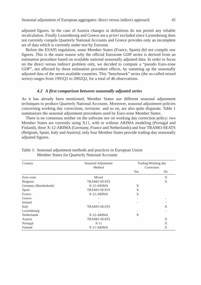
Seasonal adjustment of European aggregates: direct versus indirect approach 45
adjusted figures. In the case of Austria changes in definitions do not permit any reliablerecalculation. Finally Luxembourg and Greece are a priori excluded since Luxembourg doesnot currently compile Quarterly National Accounts and Greece provides only an incompleteset of data which is currently under test by Eurostat.
Before the ESA95 regulation, some Member States (France, Spain) did not compile rawfigures. This is the main reason why the official Eurozone GDP series is derived from anestimation procedure based on available national seasonally adjusted data. In order to focuson the direct versus indirect problem only, we decided to compute a “pseudo Euro-zoneGDP”, not affected by these estimation procedure effects, by summing up the seasonallyadjusted data of the seven available countries. This “benchmark” series (the so-called mixedseries) ranges from 1991Q1 to 2002Q2, for a total of 46 observations.
4.2 A first comparison between seasonally adjusted series
As it has already been mentioned, Member States use different seasonal adjustmenttechniques to produce Quarterly National Accounts. Moreover, seasonal adjustment policiesconcerning working day corrections, revisions and so on, are also quite disparate. Table 1summarizes the seasonal adjustment procedures used by Euro-zone Member States.
There is no consensus neither on the software nor on working day correction policy: twoMember States are currently using X11, with or without ARIMA modeling (Portugal andFinland), three X-12-ARIMA (Germany, France and Netherlands) and four TRAMO-SEATS(Belgium, Spain, Italy and Austria); only four Member States provide trading-day seasonallyadjusted figures.
Table 1: Seasonal adjustment methods and practices in European UnionMember States for Quarterly National Accounts
Country Seasonal Adjustment Trading/Working dayMethod Correction
Yes No
Euro-zone Mixed XBelgium TRAMO-SEATS XGermany (Bundesbank) X-12-ARIMA XSpain TRAMO-SEATS XFrance X-12-ARIMA XGreece - - -Ireland - - -Italy TRAMO-SEATS XLuxembourg - - -Netherlands X-12-ARIMA XAustria TRAMO-SEATS XPortugal X-11 XFinland X-11-ARIMA X

46 Ladiray and Mazzi
Figure 1 presents the mixed adjustment and the TRAMO-SEATS direct and indirectseasonally adjusted series. It is very difficult to detect a real difference between the threeseries (and it will be the same with the X-12-ARIMA estimates). This similarity is confirmedby the numerical indicators displayed in Table 2. The mean absolute percentage differencebetween two estimates is quite small: less than 0.1% between direct and indirect, and close to0.2% between the mixed and the other estimates.
Table 2: Absolute percentage deviation indicators (GDP geographical aggregation)
Indicator Ind. vs Dir. Best Ind. vs Mixed Dir. vs MixedT-S X-12 T-S X-12 T-S X-12
Mean APD (SA) 0.068 0.067 X12ar 0.180 0.168 0.214 0.207Max APD (SA) 0.395 0.414 Seats 0.587 0.652 0.924 0.804Mean APD (SA), Last 3 years 0.029 0.070 Seats 0.169 0.154 0.161 0.214Max APD (SA), Last 3 years 0.051 0.316 Seats 0.350 0.399 0.323 0.446Mean APD (TC) 0.060 0.109 Seats 0.132 0.184 0.173 0.150Max APD (TC) 0.809 1.378 Seats 0.598 1.924 0.863 0.599Mean APD (TC), Last 3 years 0.018 0.053 Seats 0.111 0.147 0.121 0.195Max APD (TC), Last 3 years 0.045 0.133 Seats 0.257 0.251 0.269 0.368Mean APD (S) 0.076 0.067 X12ar 0.165 0.168 0.214 0.207Max APD (S) 0.443 0.415 X12ar 0.611 0.656 0.933 0.811Mean APD (S), Last 3 years 0.033 0.070 Seats 0.149 0.154 0.161 0.214Max APD (S), Last 3 years 0.098 0.317 Seats 0.342 0.397 0.324 0.444
Figure 1: Mixed and TRAMO-SEATS direct and indirect adjustments:GDP geographical aggregation(millions)
1.4
1.3
1.2
1.1
1.0
0.9
0.7
0.8
1.4
1.3
1.2
1.1
1.0
0.9
0.7
0.8
1980 1982 1984 1986 1988 1990 1992 1994 1996 1998 2000 2002 2004
Mixed adjustmentsTRAMO-SEATS direct adjustmentsTRAMO-SEATS indirect adjustments

Seasonal adjustment of European aggregates: direct versus indirect approach 47
Figure 2: Growth rates of mixed, TRAMO-SEATS direct and indirect adjustments:GDP geographical aggregation
1980 1982 1984 1986 1988 1990 1992 1994 1996 1998 2000 2002
3
2
1
0
-1
-2
3
2
1
0
-1
-2
Growth rates of mixedTRAMO-SEATS DirectIndirect
Figure 3: Growth rates of mixed, X-12-ARIMA direct and indirect adjustments:GDP geographical aggregation
1980 1982 1984 1986 1988 1990 1992 1994 1996 1998 2000 2002
3
2
1
0
-1
-2
3
2
1
0
-1
-2
Growth rates of mixedX-12-ARIMA DirectIndirect

48 Ladiray and Mazzi
Figure 5: Relative differences of mixed aggregate versus direct and indirect adjustments:GDP geographical aggregation. X-12-ARIMA
1991 1992 1993 1994 1995 1996 1997 1998 1999 2000 2001 2002 2003
1.0
0.5
0.0
-0.5
-1.0
1.0
0.5
0.0
-0.5
-1.0
Relative differences of mixed aggregate vs. directIndirect
Figure 4: Relative differences of mixed aggregate versus direct and indirect adjustments:GDP geographical aggregation. TRAMO-SEATS
1991 1992 1993 1994 1995 1996 1997 1998 1999 2000 2001 2002 2003
1.0
0.5
0.0
-0.5
-1.0
1.0
0.5
0.0
-0.5
-1.0
Relative differences of mixed aggregate vs. directIndirect

Seasonal adjustment of European aggregates: direct versus indirect approach 49
The growth rates, which are in this case of greater interest, are displayed in Figures 2 and 3.Finally, Figures 4 and 5 show the relative difference of the mixed benchmark series withrespect to the direct and indirect seasonal adjusted series obtained with TRAMO-SEATS andX-12-ARIMA.
The key elements emerging from this set of pictures can be synthesized as follows:• direct and indirect adjusted series have a very similar behaviour, regardless to the software
used (X-12-ARIMA or TRAMO-SEATS);• 1993Q1 and 1997Q1 appear to be very special quarters where direct and indirect estimates
show a much more important decrease in the GDP than mixed approach;• the X-12-ARIMA estimates are slightly closer to the mixed estimate than those obtained
with TRAMO-SEATS. This is certainly a direct consequence of the use of the Census filterin the large majority of Member States.To complete this comparison, Table 3 presents some descriptive statistics on the differences
between growth rates of the various approaches. Differences close to zero with little varianceindicate a good agreement between the different estimates. This is the case as all averagedifferences are very small. One must note that, as far as variances and ranges are concerned,the indirect approaches are closer to the mixed approach than the direct approaches; the X-12-ARIMA indirect estimate gets the best results.
4.3 Concordance analysis of growth rates
Short-term analysts are mainly interested in the evolution of macroeconomic aggregates andtherefore in growth rates of seasonally adjusted data. It is important that different seasonaladjusted data do not provide users with inconsistent messages.
Tables 4 and 5 detail the cases of discrepancies in sign between the various aggregates andwith their sub-components, according to the adjustment approach.
Direct and indirect estimates only disagree, i.e. give an opposite evolution of the indicator,in two cases out of 89 for TRAMO-SEATS (1982Q1 and 1986Q1) and in one case for X-12-Arima (1995Q3). This leads to high concordance rates between the two approaches, namely97.75% for TRAMO-SEATS and 98.88% for X-12-ARIMA. Furthermore, one should noticethat these discrepancies concern growth rates close to zero.
The discrepancies are more numerous in the comparison with the mixed approach even ifthe global concordance rate remains good. 1991Q3 and 1993Q2 are strong inconsistencies forany software and approach. In these cases, the mixed series slightly decreases (-0.064% and-0.010%) when direct and indirect approach increase. The other inconsistencies concernsmaller growth rates. The highest number of inconsistencies is given by a direct approachusing X-12-ARIMA.
Table 3: Differences in growth rates between the three approaches:GDP geographical aggregation
Indicator Dir. vs Ind. Mixed vs Ind. Mixed vs Dir.T-S X-12 T-S X-12 T-S X-12
Mean -0.001 -0.005 -0.013 -0.009 -0.020 -0.013Minimum -0.729 -0.511 -0.925 -1.131 -0.853 -1.311Maximum 0.304 0.538 0.686 0.686 1.158 0.689Variance 0.027 0.023 0.104 0.098 0.151 0.149Range 1.033 1.049 1.611 1.817 2.011 1.999

50 Ladiray and Mazzi
Table 4: Inconsistencies in growth rates between the three approaches:GDP geographical aggregation
Direct vs IndirectTRAMO-SEATS X-12-ARIMA
Date Direct Indirect Date Direct Indirect
1982Q1 0.007 -0.023 1995Q3 -0.043 0.0461986Q1 0.034 -0.072
Mixed vs DirectTRAMO-SEATS X-12-ARIMA
Date Mixed Direct Date Mixed Direct
1991Q3 -0.064 0.516 1991Q3 -0.064 0.3421992Q3 -0.18 0.44 1992Q3 -0.18 0.3361993Q2 -0.01 0.692 1993Q2 -0.01 0.5691997Q1 0.298 -0.104 1995Q3 0.17 -0.043
1997Q1 0.298 -0.391
Mixed vs IndirectTRAMO-SEATS X-12-ARIMA
Date Mixed Indirect Date Mixed Indirect
1991Q3 -0.064 0.383 1991Q3 -0.064 0.2491992Q3 -0.18 0.23 1992Q3 -0.18 0.2671993Q2 -0.01 0.465 1993Q2 -0.01 0.3311997Q1 0.298 -0.169 1997Q1 0.298 -0.193
The inconsistencies between the evolution of an aggregate and the majority of itscomponents are presented, for the different approaches and programs, in Table 5.
Table 6 presents the concordance rates between the various approaches, a statistic thatsummarizes the previous elements. The results are quite similar for the two programs: theconcordance rate is very high between the direct and the indirect approaches, slightly lower inthe other cases.

Seasonal adjustment of European aggregates: direct versus indirect approach 51
TRAMO-SEATS X-12-ARIMA
Direct and Indirect 97.75 98.88Direct and Components 93.26 92.13Indirect and Components 93.26 93.26
Mixed and Direct 91.11 88.89Mixed and Indirect 91.11 91.11
Mixed and Components 95.56
Table 6: Concordance rates (in %): GDP geographical aggregation
Direct or Indirect, TRAMO-SEATSDate Direct Indirect Weights BE DE ES FR IT FI NL
1981 Q1 -0.107 -0.079 0.614 -0.56 0.09 -0.13 0.11 -0.47 1.02 -0.531981 Q4 0.263 0.312 0.471 -0.07 -0.27 -0.06 1.16 0.52 1.29 -0.271982 Q1 0.007 -0.023 0.613 0.14 -0.60 0.60 0.16 0.35 0.41 -0.021983 Q3 0.282 0.212 0.412 0.71 -0.20 0.03 -0.16 1.31 0.83 0.411986 Q1 0.034 -0.072 0.426 -0.21 -0.33 0.44 0.07 -0.26 -0.38 0.691990 Q2 0.406 0.195 0.486 -0.79 0.46 1.09 -0.12 -0.05 -0.96 0.691995 Q3 0.125 0.071 0.363 0.01 -0.17 0.57 -0.02 0.24 -0.12 0.79
Direct or Indirect, X-12-Arima
Date Direct Indirect Weights BE DE ES FR IT FI NL
1980 Q4 0.085 0.157 0.343 -0.24 -0.55 0.80 -0.38 0.70 -0.83 4.071981 Q1 -0.094 -0.116 0.660 0.02 0.19 -0.57 0.45 -0.46 1.10 -2.671983 Q3 0.314 0.270 0.321 0.72 -0.21 -0.08 -0.00 1.07 0.72 1.551987 Q1 -0.310 -0.238 0.618 0.93 -1.97 2.19 0.39 0.42 0.53 -0.461990 Q2 0.090 0.018 0.162 -0.45 -0.08 1.24 -0.13 -0.11 -1.02 0.391995 Q3 -0.043 0.046 0.616 0.66 -0.38 0.08 0.16 0.24 0.22 1.121996 Q4 0.059 0.050 0.221 0.63 -0.02 0.56 -0.27 -0.04 1.06 0.44
Mixed Approach
Date Mixed Weights BE DE ES FR IT FI NL
1991 Q3 -0.064 0.598 0.53 -0.69 0.37 0.18 0.63 -1.29 0.322001 Q3 0.146 0.358 -0.03 -0.19 1.01 0.40 -0.02 1.34 -0.10
Table 5: Inconsistencies in growth rates between aggregate and components:GDP geographical aggregation(If weights is greater than 0.5 (less than 0.5), the main part of the national GDP increases (decreases)).

52 Ladiray and Mazzi
TRAMO-SEATS X-12-ARIMA MixedIndicator Direct Indirect Direct Indirect adjustment
M1* 0.028 0.039 0.036 0.070 0.012M2* 0.034 0.051 0.068 0.105 0.031M3* 0.000 0.000 0.000 0.000 0.000M4 0.131 0.131 0.261 1.045 0.692M5 0.200 0.200 0.200 0.200 0.200M7* 0.769 2.035 1.828 2.108 0.856M8 0.571 0.567 0.246 0.531 1.691M9 0.174 0.173 0.156 0.124 0.188M10 0.525 0.466 0.139 0.404 1.531M11 0.444 0.263 0.139 0.387 1.279Q 0.298 0.544 0.469 0.646 0.533
Table 7: Quality measures: GDP geographical aggregation
4.4 Quality measures of seasonal adjustments
A comparison between the various adjustments can be also made with respect to the so-calledquality measures proposed by X-12-ARIMA and here extended, where possible, to TRAMO-SEATS estimates and to the mixed approach. The results are presented in Table 7.
The M and Q statistics are commonly analyzed by statisticians in order to have a syntheticview of the performance of their adjustment: a value greater than one, for any of thesestatistics, indicates a possible problem in the seasonal adjustment. Table 7 does not shownsignificant differences among the approaches. The only case where none of the M statisticsexceed the critical value is the direct adjustment with TRAMO-SEATS.
All the other approaches seem to present some problems concerning the M7 statistics,measuring wether the seasonal pattern in the series tends to remain constant over time or not.Furthermore the level of M4 for the indirect approach using X-12-ARIMA shows how theirregular component displays some residual autocorrelation.
4.5 Roughness measures
Roughness measures are presented in Table 8 and refer to the seasonally adjusted series, thetrend-cycle and the seasonal component. The smoothness of seasonally adjusted data is oftenconsidered as one of the most important criteria from the users point of view. Nevertheless, itmust be stressed, as mentioned in Section 4, that this criterion has to be used carefully: theirregular component is an integral part of the series and it seems quite strange to prefer theseries that presents the smallest irregular!
A first very simple conclusion we can draw from this table is that there is no clear evidencein favor of one of the approaches:• the mixed approach gives, on the whole period, the smoother seasonally adjusted series and
the smoother trend;• X-12-ARIMA gets better results with the direct approach (in 9 cases out of 12) and on the
opposite, for TRAMO-SEATS the indirect adjustment gives better results in all the cases;• as far as the smoothness of the seasonal component is concerned, X-12-ARIMA gives the
best results and the mixed approach the worse.

Seasonal adjustment of European aggregates: direct versus indirect approach 53
Indicator TRAMO-SEATS X-12-ARIMA Direct vs IndirectDirect Indirect Direct Indirect SEATS X-12
Mean AR 1 qtr 0.126 0.088 0.083 0.062 I IMean AR 2 qtrs 0.152 0.127 0.109 0.074 I IMean AR 3 qtrs 0.165 0.126 0.117 0.075 I IMean AR 4 qtrs 0.214 0.134 0.161 0.111 I IMean AR 5 qtrs 0.226 0.122 0.149 0.099 I IStd AR 1 qtr 0.119 0.062 0.077 0.048 I IStd AR 2 qtrs 0.104 0.069 0.109 0.057 I IStd AR 3 qtrs 0.125 0.072 0.117 0.058 I IStd AR 4 qtrs 0.112 0.069 0.103 0.055 I IStd AR 5 qtrs 0.162 0.069 0.109 0.054 I ISliding SpansA(%) 0.000 0.000 0.000 0.000 = =MM(%) 1.266 1.266 0.000 0.000 = =
Table 9: Absolute revisions (mean and standard deviation in %) and sliding spansanalysis: GDP geographical aggregation
TRAMO-SEATS X-12-ARIMA MixedDirect Indirect Direct Indirect approach SEATS X-12
R1 (SA) 11415.1 11868.9 12274.3 12222.7 8025.2 D IR1 (SA), Last 3 years 7038.7 7128.3 7776.6 7229.3 7167.2 D IR2 (SA) 0.245 0.271 0.289 0.289 0.106 D IR2 (SA), Last 3 years 0.112 0.117 0.136 0.132 0.083 D IR3 (SA) 0.178 0.216 0.250 0.310 0.106 D DR3 (SA), Last 3 years 0.137 0.142 0.154 0.145 0.083 D IMar (TC, 1) 10948.9 11303.7 11221.9 9800.7 7420.9 D IMar (TC, 1), Last 3 years 8317.1 8395.4 9236.2 8913.5 8766.3 D IMar (TC, 2) 11195.8 12089.6 11497.4 6332.2 3219.7 D IMar (TC, 2), Last 3 years 2373.8 2573.9 4063.9 3380.4 2596.1 D IMar (S) 0.018 0.019 0.009 0.017 0.051 D DMar (S), Last 3 years 0.017 0.018 0.005 0.014 0.052 D D
Table 8: Roughness measures: GDP geographical aggregation
4.6 Revision analysis
Users prefer to deal with seasonally adjusted time series which are revised as few as possible.Non revised seasonally adjusted figures could be obtain with purely asymmetric filters (withthe DAINTIES method for example) but with a possible serious counterpart: a phase shift inturning point detection.
Table 9 presents the revisions of direct and indirect estimates obtained with the twosoftwares. It is important to note that this revision analysis concentrates on revisions inducedby the seasonal adjustment process:• for the simulations, the ARIMA model and the decomposition model have been fixed;• revisions of raw data which occur regularly, as new information became available have not
been taken into account.The results are very clear and speak in favour of the indirect approach, both for TRAMO-
SEATS and for X-12-ARIMA.
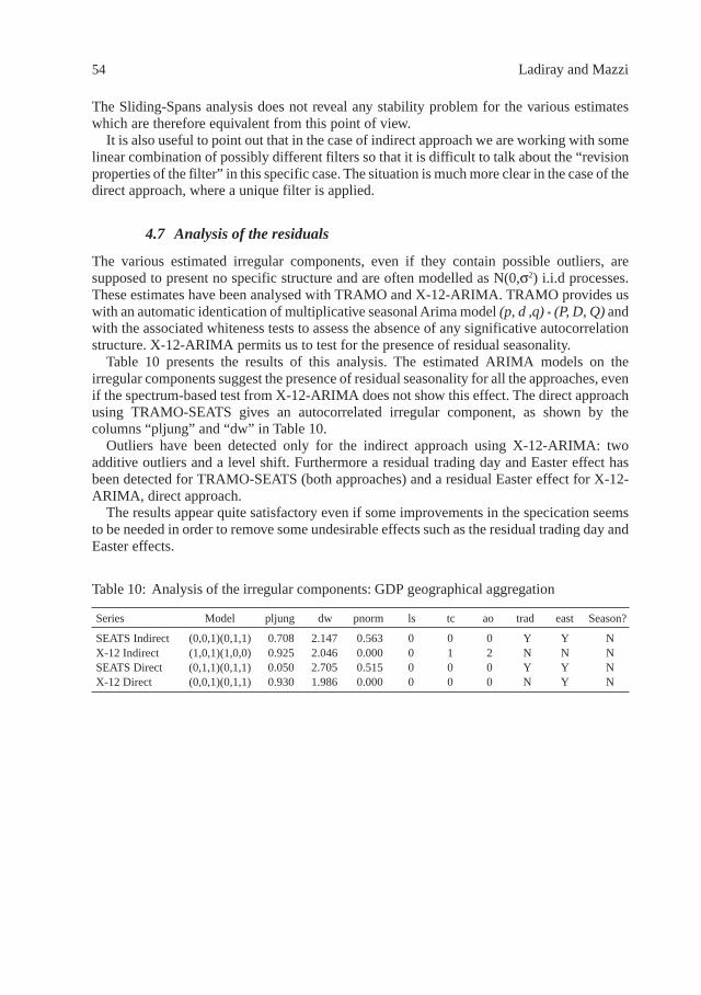
54 Ladiray and Mazzi
Series Model pljung dw pnorm ls tc ao trad east Season?
SEATS Indirect (0,0,1)(0,1,1) 0.708 2.147 0.563 0 0 0 Y Y NX-12 Indirect (1,0,1)(1,0,0) 0.925 2.046 0.000 0 1 2 N N NSEATS Direct (0,1,1)(0,1,1) 0.050 2.705 0.515 0 0 0 Y Y NX-12 Direct (0,0,1)(0,1,1) 0.930 1.986 0.000 0 0 0 N Y N
Table 10: Analysis of the irregular components: GDP geographical aggregation
The Sliding-Spans analysis does not reveal any stability problem for the various estimateswhich are therefore equivalent from this point of view.
It is also useful to point out that in the case of indirect approach we are working with somelinear combination of possibly different filters so that it is difficult to talk about the “revisionproperties of the filter” in this specific case. The situation is much more clear in the case of thedirect approach, where a unique filter is applied.
4.7 Analysis of the residuals
The various estimated irregular components, even if they contain possible outliers, aresupposed to present no specific structure and are often modelled as N(0,σ2) i.i.d processes.These estimates have been analysed with TRAMO and X-12-ARIMA. TRAMO provides uswith an automatic identication of multiplicative seasonal Arima model (p, d ,q) * (P, D, Q) andwith the associated whiteness tests to assess the absence of any significative autocorrelationstructure. X-12-ARIMA permits us to test for the presence of residual seasonality.
Table 10 presents the results of this analysis. The estimated ARIMA models on theirregular components suggest the presence of residual seasonality for all the approaches, evenif the spectrum-based test from X-12-ARIMA does not show this effect. The direct approachusing TRAMO-SEATS gives an autocorrelated irregular component, as shown by thecolumns “pljung” and “dw” in Table 10.
Outliers have been detected only for the indirect approach using X-12-ARIMA: twoadditive outliers and a level shift. Furthermore a residual trading day and Easter effect hasbeen detected for TRAMO-SEATS (both approaches) and a residual Easter effect for X-12-ARIMA, direct approach.
The results appear quite satisfactory even if some improvements in the specication seemsto be needed in order to remove some undesirable effects such as the residual trading day andEaster effects.

Seasonal adjustment of European aggregates: direct versus indirect approach 55
5 Gross domestic product, aggregation by sector
In this application, we consider that the Euro-zone GDP at constant prices can also be seen asthe sum of the gross value added of the six main branches in the NACE Rev. 1 classificationand of a “Taxes minus FISIM” component. The direct vs indirect analysis performed in thisSection is conditioned to the adoption of a direct approach for the geographical aggregation.
5.1 The data
The seven components we have considered in this application are:1. Agriculture, hunting, forestry and shing;2. Total industry, excluding construction;3. Construction;4. Wholesale and retail trade;5. Financial Intermediation;6. Public administration;7. Taxes minus FISIM.
The raw Member State series for each branch were summed up to obtain a “pseudo” Euro-zone aggregate for the considered branch. The same operation was done with seasonallyadjusted data to obtain the corresponding mixed aggregate. Because of data availability, theexercise takes into account six countries only – Belgium, Germany, Spain, Finland, Franceand Italy – and the data range from 1980Q1 to 2002Q2 (90 observations). These countriesrepresent more than 86% of the Euro-zone GDP. In this simulation the Netherlands isexcluded because the breakdown by sector is available just for a shorter period.
5.2 A first comparison between seasonally adjusted series
Figure 6 presents the mixed adjustment and the TRAMO-SEATS direct and indirectseasonally adjusted series. It is, like for the geographical aggregation case, very difficult todetect a real difference between the three series (and it will be the same with the X-12-ARIMA estimates). This similarity is confirmed by the numerical indicators displayed inTable 11. The mean absolute percentage difference between two estimates is very small, andsmaller than for the geographical aggregation case: less than 0.1% between direct andindirect, and close to 0.2% between the mixed and the other estimates. The direct versusindirect problem is therefore not very important.

56 Ladiray and Mazzi
Indicator Ind. vs Dir. Best Ind. vs Mixed Dir. vs MixedT-S X-12 T-S X-12 T-S X-12
Mean APD (SA) 0.042 0.041 X12ar 0.170 0.178 0.147 0.179Max APD (SA) 0.231 0.209 X12ar 0.841 0.988 0.712 1.001Mean APD (SA), Last 3 years 0.025 0.057 Seats 0.108 0.157 0.105 0.174Max APD (SA), Last 3 years 0.077 0.161 Seats 0.395 0.582 0.411 0.685Mean APD (TC) 0.059 0.100 Seats 0.165 0.176 0.124 0.126Max APD (TC) 0.443 1.873 Seats 0.632 1.774 0.611 0.693Mean APD (TC), Last 3 years 0.030 0.063 Seats 0.064 0.081 0.063 0.057Max APD (TC), Last 3 years 0.055 0.157 Seats 0.203 0.162 0.198 0.164Mean APD (S) 0.399 0.240 X12ar 0.491 0.332 0.147 0.178Max APD (S) 1.467 0.973 X12ar 2.195 1.656 0.718 0.731Mean APD (S), Last 3 years 0.449 0.245 X12ar 0.529 0.370 0.105 0.185Max APD (S), Last 3 years 1.293 0.826 X12ar 1.495 1.240 0.409 0.633
Table 11: Absolute percentage deviation indicators (GDP aggregation by sector)
Figure 6: Mixed, TRAMO-SEATS direct and indirect adjustments:GDP aggregation by sector(millions)
1.5
1.4
1.3
1.2
1.1
1.0
0.8
0.9
1.5
1.4
1.3
1.2
1.1
1.0
0.8
0.9
1980 1982 1984 1986 1988 1990 1992 1994 1996 1998 2000 2002 2004
MixedTRAMO-SEATS directIndirect

Seasonal adjustment of European aggregates: direct versus indirect approach 57
Figure 7: Growth rates of mixed and TRAMO-SEATS direct and indirect adjustments:GDP aggregation by sector
1980 1982 1984 1986 1988 1990 1992 1994 1996 1998 2000 2002
3
2
1
0
-1
-2
3
2
1
0
-1
-2
Growth rates of mixedTRAMO-SEATS directIndirect
1980 1982 1984 1986 1988 1990 1992 1994 1996 1998 2000 2002
3
2
1
0
-1
-2
3
2
1
0
-1
-2
Growth rates of mixedTRAMO-SEATS directIndirect
Figure 8: Growth rates of mixed and X-12-ARIMA direct and indirect adjustments:GDP aggregation by sector

58 Ladiray and Mazzi
Figure 9: Relative differences of mixed aggregate versus direct and indirect adjustments:GDP aggregation by sector. TRAMO-SEATS
1991 1992 1993 1994 1995 1996 1997 1998 1999 2000 2001 2002 2003
1.0
0.5
0.0
-0.5
-1.0
1.0
0.5
0.0
-0.5
-1.0
Mixed aggregate versus direct adjustmentsIndirect adjustments
Figure 10: Relative differences of mixed aggregate versus direct and indirect adjustments:GDP aggregation by sector. X-12-ARIMA
1991 1992 1993 1994 1995 1996 1997 1998 1999 2000 2001 2002 2003
1.0
0.5
0.0
-0.5
-1.0
1.0
0.5
0.0
-0.5
-1.0
Mixed aggregate versus direct adjustmentsIndirect adjustments

Seasonal adjustment of European aggregates: direct versus indirect approach 59
Indicator Dir. vs Ind. Mixed vs Ind. Mixed vs Dir.T-S X-12 T-S X-12 T-S X-12
Mean 0.000 0.000 -0.006 -0.002 -0.004 -0.001Minimum -0.221 -0.332 -0.745 -0.960 -0.626 -1.002Maximum 0.391 0.245 0.673 1.049 0.759 1.313Variance 0.009 0.008 0.081 0.127 0.062 0.145Range 0.611 0.577 1.418 2.009 1.385 2.315
Table 12: Differences in growth rates between the three approaches:GDP aggregation by sector
The growth rates are displayed in Figures 7 and 8. Finally, Figures 9 and 10 show therelative difference of the mixed benchmark series with respect to the direct and indirectseasonal adjusted series obtained with TRAMO-SEATS and X-12-ARIMA.
The main conclusions we can draw from this set of pictures are the following:• direct and indirect adjusted series have a very similar behaviour, regardless to the software
(X-12-ARIMA or TRAMO-SEATS);• 1993Q1 appears to be a very special date where direct and indirect estimates show a much
more important decrease in the GDP than mixed approach;• the X-12-ARIMA estimates are closer to the mixed estimate than those obtained with
TRAMO-SEATS. This is certainly a direct consequence of the use of the Census filter inthe large majority of Member States.Table 12 statistics confirm the good agreement between the different estimates: all average
differences are very small. One must notice that the direct approaches are closer to the mixedapproach than the indirect ones.
5.3 Concordance analysis of growth rates
Tables 13 and 14 detail the cases of discrepancies in sign of the growth rates obtained fromthe various adjustment approaches.
Direct and indirect estimates only disagree, e.g. give an opposite indication of the evolutionof the indicator, in two cases out of 89 observations. But these discrepancies concern growthrates close to zero.
The discrepancies are more numerous when comparing with the mixed approach. X-12-ARIMA performs worse than TRAMO-SEATS. 1991Q3 is a strong inconsistency for anysoftware and approach: the mixed series slightly decreases (-0.1%) when direct and indirectapproaches increase (around 0.4%). The number of large discrepancies (i.e. higher than 0.5percentage points) differs according to the approach: one for TRAMO-SEATS/direct, threefor X-12-ARIMA/direct, three for TRAMO-SEATS/indirect and four for X-12-ARIMA/indirect.
The inconsistencies between the evolution of an aggregate and the majority of itscomponents are presented, for the different approaches and programs, in Table 14.
TRAMO-SEATS presents six inconsistencies for the direct estimate and four for theindirect one. X-12-ARIMA presents five inconsistencies for the direct estimate and three forthe indirect one. The mixed approach presents two inconsistencies in 1992Q3 and 1995Q4.

60 Ladiray and Mazzi
TRAMO-SEATS X-12-ARIMADirect vs Indirect
Date Direct Indirect Date Direct Indirect1992 Q2 0.073 -0.046 1992 Q3 0.023 -0.0351992 Q3 0.068 -0.003 1996 Q4 -0.055 0.007
Mixed vs DirectDate Mixed Direct Date Mixed Direct
1991 Q3 -0.089 0.484 1991 Q3 -0.089 0.3431993 Q2 -0.047 0.347 1991 Q4 0.82 -0.0211996 Q1 0.153 -0.064 1992 Q2 -0.671 0.33
1993 Q2 -0.047 0.3181996 Q1 0.153 -0.592000 Q1 0.91 -0.403
Mixed vs IndirectDate Mixed Indirect Date Mixed Indirect
1991 Q3 -0.089 0.586 1991 Q3 -0.089 0.4371992 Q2 -0.671 0.073 1991 Q4 0.82 -0.0771992 Q3 -0.208 0.068 1992 Q2 -0.671 0.2891993 Q2 -0.047 0.491 1992 Q3 -0.208 0.0231996 Q1 0.153 -0.155 1993 Q2 -0.047 0.244
1996 Q1 0.153 -0.6031996 Q4 0.209 -0.0552000 Q1 0.91 -0.139
Table 13: Inconsistencies in growth rates between the three approaches:GDP aggregation by sector

Seasonal adjustment of European aggregates: direct versus indirect approach 61
Direct or Indirect, TRAMO-SEATSDate Direct Indirect Weights AGRI IND CONS RETA FINAN PUBL TAXES FISIM
1984Q4 0.206 0.328 0.333 -2.22 1.08 -0.67 -0.04 0.85 0.07 -0.04 0.451992Q2 -0.046 0.073 0.667 0.77 -0.41 0.15 -0.12 0.53 0.23 0.06 0.261992Q3 -0.003 0.068 0.833 1.00 -1.36 0.34 -0.16 0.55 0.85 0.62 -0.211992Q4 -0.390 -0.220 0.667 -0.52 -2.28 0.31 -0.06 0.36 0.01 2.04 -0.351995Q4 0.139 0.159 0.333 2.95 -0.23 -0.80 -0.25 0.85 0.60 -0.58 0.841996Q4 0.065 0.016 0.333 -1.86 -0.50 -0.92 0.52 0.76 0.11 -0.62 0.58
Direct or Indirect, X-12-ARIMADate Direct Indirect Weights AGRI IND CONS RETA FINAN PUBL TAXES FISIM
1984Q4 0.246 0.274 0.167 -1.16 0.98 -0.95 -0.22 0.96 -0.02 -0.12 0.551988Q1 0.296 0.234 0.333 -1.48 0.92 -0.01 0.58 -0.28 -0.13 0.44 0.211992Q3 -0.035 0.023 0.667 1.42 -1.45 -1.02 -0.25 0.81 0.98 0.44 -0.121995Q4 0.126 0.113 0.333 2.55 -0.45 -0.95 -0.35 0.84 0.71 -0.35 0.951996Q4 0.007 -0.055 0.333 -1.67 -0.63 -1.57 0.45 0.62 0.15 -0.37 0.562001Q2 -0.021 -0.067 0.667 -1.17 -0.89 0.11 0.05 0.46 0.27 0.18 1.13
Mixed ApproachDate Mixed Weights AGRI IND CONS RETA FINAN PUBL TAXES FISIM
1992Q3 -0.208 0.667 1.65 -1.75 -1.00 -0.60 0.56 0.65 0.52 -0.401995Q4 0.047 0.333 2.13 -0.35 -0.76 -0.36 0.82 0.57 -0.97 0.77
Table 14: Inconsistencies in growth rates between aggregate and components:GDP aggregation by sector(If weights is greater than 0.5 (less than 0.5), the main part of the national GDP increases (decreases))
Table 15 presents the concordance rates between the various approaches, a statistic thatsummarizes the previous elements. The concordance rate of the direct/indirect approacheswith respect to the mixed one are higher for TRAMO-SEATS than for X-12-ARIMA. Theyare all satisfactory except for the concordance between the mixed approach and the indirectapproach using X-12-ARIMA.
Tramo-Seats X-12-Arima
Direct and Indirect 97.75 97.75Direct and Components 93.26 93.26Indirect and Components 95.51 95.51
Mixed and Direct 93.33 86.67Mixed and Indirect 88.89 82.22
Mixed and Components 95.56
Table 15: Concordance rates: GDP aggregation by sector(in %)

62 Ladiray and Mazzi
5.4 Quality measures of seasonal adjustments
The M and Q-statistics results are presented in Table 16. All the approaches present someproblems concerning the M7 statistics, so the seasonal pattern in the series is not constantover the sample period. Furthermore the indirect approaches present high values of M8, M10and M11, indicating that large variations in the magnitude of the seasonal component arerecorded, especially in the last three years of the series. The high value of M4 for the indirectadjustment using X-12-ARIMA suggests the presence of autocorrelation in the residuals, aresult which is also confirmed by Table 19.
5.5 Roughness measures
Roughness measures are presented in Table 17 and refer to the seasonally adjusted series, tothe trend-cycle and to the seasonal component.
A first very simple conclusion we can draw from this table is that, once more, there is noclear evidence in favor of one of the approaches. In particular, we may notice how:• in general the indirect approaches seem to give smoother seasonally adjusted series,
following the R1 and R2 statistics, even if R3 gives the opposite results. For TRAMO-SEATS we get to the opposite conclusion if we consider only the last three years of thesample;
• the indirect approaches give also the smoother Trend-Cycles, even if for X-12-ARIMA thedirect approach seems preferrable when considering only the last three years;
• the direct approaches provide the smoother seasonal factors.Anyway the differences between direct and indirect are too small to be considered as
relevant, especially for TRAMO-SEATs.
Indicator TRAMO-SEATS X-12-ARIMA MixedDirect Indirect Direct Indirect adjustment
M1* 0.015 0.023 0.027 0.076 0.015M2* 0.016 0.025 0.033 0.107 0.034M3* 0.000 0.000 0.000 0.000 0.000M4 0.751 0.555 0.849 1.045 0.969M5 0.200 0.200 0.200 0.200 0.200M7* 2.256 2.158 2.523 3.344 0.105M8 0.485 3.087 0.397 1.918 1.338M9 0.183 0.219 0.204 0.171 0.143M10 0.408 2.710 0.363 1.621 1.045M11 0.345 1.937 0.363 1.288 0.624Q 0.631 0.968 0.691 1.031 0.327
Table 16: Quality measures

Seasonal adjustment of European aggregates: direct versus indirect approach 63
Indicator TRAMO-SEATS X-12-ARIMA Direct vs IndirectDirect Indirect Direct Indirect SEATS X-12
Mean AR 1 qtr 0.157 0.129 0.170 0.131 I IMean AR 2 qtrs 0.157 0.131 0.189 0.135 I IMean AR 3 qtrs 0.160 0.134 0.204 0.136 I IMean AR 4 qtrs 0.156 0.130 0.187 0.127 I IMean AR 5 qtrs 0.158 0.137 0.198 0.144 I IStd AR 1 qtr 0.090 0.082 0.110 0.075 I IStd AR 2 qtrs 0.097 0.085 0.119 0.072 I IStd AR 3 qtrs 0.091 0.081 0.105 0.064 I IStd AR 4 qtrs 0.096 0.086 0.153 0.105 I IStd AR 5 qtrs 0.089 0.084 0.146 0.098 I I
Sliding SpansA (%) 3.659 1.220 0.000 0.000 = =MM (%) 1.236 1.236 3.704 3.704 = =
Table 18: Absolute revisions (mean and standard deviation in %) and sliding spansanalysis: GDP aggregation by sector
5.6 Revision analysis
Table 18 presents the revisions of direct and indirect estimates obtained with the twoprograms. Both for TRAMO-SEATS and for X-12-ARIMA the indirect approach performsbetter both in terms of mean and variance of the revisions, even if the difference between thetwo approaches is smaller for TRAMO-SEATS than for X-12-ARIMA.
The Sliding-Spans analysis reveals a small problem of instability for the direct approachusing TRAMO-SEATS (3.7% of dates have unstable adjustments) and for both approachesusing X-12-ARIMA (3.7% of dates have unstable month-to-month percent changes).
Table 17: Roughness measures: GDP aggregation by sector
TRAMO-SEATS X-12-ARIMA MixedDirect Indirect Direct Indirect approach SEATS X-12
R1 (SA) 11278.1 11060.7 11816.8 11749.4 7479.3 I IR1 (SA), Last 3 years 6468.5 6573.4 8163.3 7891.3 6827.6 D IR2 (SA) 0.283 0.270 0.308 0.306 0.111 I IR2 (SA), Last 3 years 0.129 0.134 0.220 0.197 0.091 D IR3 (SA) 0.124 0.156 0.181 0.323 0.111 D DR3 (SA), Last 3 years 0.120 0.128 0.227 0.214 0.091 D IMar (TC, 1) 10854.4 10508.9 11103.4 9281.7 6861.6 I IMar (TC, 1), Last 3 years 7923.0 7852.7 8211.8 8236.1 8203.4 I DMar (TC, 2) 11906.1 10877.6 12326.3 6031.0 3107.3 I IMar (TC, 2), Last 3 years 2149.2 2084.3 2327.6 2796.5 2444.8 I DMar (S) 0.015 0.079 0.011 0.051 0.062 D DMar (S), Last 3 years 0.013 0.071 0.009 0.043 0.044 D D

64 Ladiray and Mazzi
Series Model pljung dw pnorm ls tc ao trad east Season?
SEATS Indirect (1,0,0)(0,0,0) 0.527 2.009 0.042 0 1 0 Y Y NX-12 Indirect (0,0,1)(0,0,0) 0.382 2.552 0.000 0 0 0 Y Y NSEATS Direct (3,0,0)(0,0,1) 0.196 1.935 0.631 0 0 0 Y Y NX-12 Direct (0,0,1)(0,0,0) 0.535 2.038 0.000 0 0 0 Y Y N
Table 19: Analysis of the Irregular Components: GDP aggregation by sector
5.7 Analysis of the residuals
The various irregular component estimates have been analysed with TRAMO and X-12-ARIMA. Table 19 presents the results of this analysis:• no residual seasonality is detected on the irregular components, and just for the direct
approach using TRAMO-SEATS the estimated ARIMA model contains a non-zeroseasonal moving average term;
• all the estimates of the irregular component present residual Easter and trading day effects;• for what regards outliers, TRAMO identifies just one transitory change for the indirect
approach using TRAMO-SEATS.
6 Conclusion
The comparison presented in this paper shows some interesting results. The first one is thatthe figures currently published by Eurostat using the mixed indirect approach are quitedifferent with respect to those obtained by using either the direct or the indirect approaches,independently of the seasonal adjustment program. This can be viewed as a consequence ofthe different seasonal adjustment policies and options adopted by Member States to compiletheir aggregates. Moreover the mixed seasonal adjustment appears to be the less satisfactoryin terms of the different quality measures that have been analysed in this paper.
On the basis of these considerations, we may conclude that the seasonal adjustmentstrategy currently used by Eurostat in the field of Quarterly National Accounts needs to beamended in order to supply users with higher quality and more transparent results.
The second result is that there are no evident and significant differences between the directand the indirect approach, both using TRAMO-SEATS and X-12-ARIMA. In some cases theproposed quality measures seem to privilege the direct approach, in other cases the indirect.Moreover for the same group of criteria, like for roughness measures for example, thesubjective appreciation can lead to prefer one approach to the other or vice versa.
These elements apply both to the geographical and to the sectoral aggregation. Even if thedefinition of a general Eurostat strategy to compute seasonal adjusted QNA figures is outsidethe scope of this paper, a reasonable seasonal adjustment strategy emerging from the resultscan be synthesised as follows:• use of a direct approach on each aggregate for the geographical aggregation;• use of the indirect approach for the sectoral aggregation.
The indirect seasonal adjusted may be less useful for the geographical aggregation becauseit would be impossible for Eurostat to publish different seasonal adjusted figures with respectto those published by Member States. Under this constraint, the additivity of the seasonaladjusted data that one would obtain by using an indirect approach cannot be used in practice.Considering also the similarity of the results obtained with the direct/indirect methods, itseems then natural to prefer the direct approach since it is easier to implement in practice.

Seasonal adjustment of European aggregates: direct versus indirect approach 65
The use of the indirect approach for sectoral aggregation could be replaced by the use of adirect approach with redistribution of discrepancies in the case of sectoral aggregation.Nevertheless this alternative solution is only feasible under the condition that the discrepancybetween the sum of the seasonally adjusted components and the seasonally adjustedaggregate series are small. The results presented in the paper suggest, anyway, that thiscondition is fulfilled.
References
[1] Blake, A., Kapetanios, G., Weale, M. (2000), A Common European Business Cycle,Working Paper, Eurostat.
[2] Dagum, E.B. (1979), On the Seasonal Adjustment of economic Time Series Aggregates: ACase Study of the Unemployment Rate, Counting the Labor Force, National CommionEmployment and Unemployment Statistics, Appendix, 2, 317-344, Washington.
[3] European Central Bank (2000), Seasonal Adjustment of Monetary Aggregates and HICPfor the Euro Area, Working Paper.
[4] Eurostat (2000), Eurostat Recommandations Concerning Seasonal Adjustment Policy,Report of the Internal Task Force on Seasonal Adjustment.
[5] Findley, D. F., Monsell, B. C., Bell, W. R., Otto, M. C. and Chen, B. (1998), NewCapabilities and Methods of the X-12-ARIMA Seasonal Adjustment Program, Journal ofBusiness and Economic Statistics, 16, 127-177.
[6] Geweke, J. (1976), The Temporal and Sectoral Aggregation of Seasonally Adjusted TimeSeries, Proceedings of the Conference on the Seasonal Analysis of Economic Time Series,Economic Research Report ER-1, Arnold Zellner Editor, Washington.
[7] Gómez, V. (2000), Revision-based Test for Direct versus Indirect Seasonal Adjustment ofAggregated Series, Working Paper, Ministerio de Economia y Hacienda, Madrid.
[8] Gómez, V. and Maravall, A. (1999), Application of TRAMO-SEATS: Examples 2 and 4,Bundesbank Seminar, Unpublished manuscript.
[9] Gómez, V. and Maravall, A. (1997), Programs TRAMO and SEATS: Instructions for theUser, Beta version, Banco de España.
[10] Hood, C. C., Ashley, J. D. and Findley, D. F. (2000), An Empirical Evaluation of thePerformance of TRAMO-SEATS on Simulated Series, Working Paper, US Bureau ofCensus, Washington.
[11] Ladiray, D., Quenneville, B. (2001), Seasonal Adjustment with the X-11 Method, LectureNotes in Statistics, Springer-Verlag, New York.
[12] Lothian, J. and Morry, M. (1977), The Problem of Aggregation; Direct or Indirect,Working Paper, Time Series Research and Analysis Division, Statistics Canada, OttawaON, Canada.
[13] Pfefferman, D., Salama, E. and Ben-Tuvia, S. (1984), On the Aggregation of Series: ANew Look at an Old Problem, Working Paper, Bureau of Statistics, Jerusalem, Israel.
[14] Planas, C., Campolongo, F. (2000), The Seasonal Adjustment of ContemporaneouslyAggregated Series, Working Paper, Joint Research Centre of European Commission, Ispra,Italy.
[15] Scott, S., Zadrozny, P. (1999), Aggregation and Model-based Methods in SeasonalAdjustment of Labor Force Series, Journal of Business and Economic Statistics, 156-161.
[16] Scott, S. (1984), A Case Study of Direct and Indirect Seasonal Adjustment of AggregateSeries, Journal of Business and Economic Statistics, 686-691.
[17] U.S. Census Bureau (2001), X-12-ARIMA Reference Manual, Version 0.2.8,Washington DC, U.S. Bureau of the Census.

66 Ladiray and Mazzi

4
Criteria to determine the optimal revision policy:a case study based on euro zone monetary aggregates data
Laurent Maurin
Introduction
Seasonal factors are only estimate, so are seasonally adjusted (SA) data. At the extremities ofa time series, the symmetric filters used to produce SA data in the cases of X12 and SEATSrequire forecasting. Hence, each time a new observation is added, the substitution of theactual value for the previous forecasted one and the production of new forecasts lead to avariation in the SA data, not only for the last previous one. Moreover, original data and in thecase of SEATS, the model, can be revised too.
This implies the need to define a revision policy in the context of recurrent publications ofSA data. The revision policy is defined as the process used to update the estimates of thepublished SA data. In consequence, the frequency of revisions is only determined by therevision policy of SA data. But the intensity of the revisions depends also on the quality of theforecasts used to extend the series at the end of the sample. As it seems plausible that thequality of forecasts increases with the frequency of updates of the underlying model, there isa trade-off between the cost of revisions and the quality of data published.
The interest of the study presented here arises from this trade-off. This trade-off might becontingent to the time series, as they behave differently. So the problem is contemplated froman empirical point of view, using Euro-aggregated monetary statistics. The two main methodsare considered: X12 and SEATS. To concentrate only on seasonal filters, they are applied tothe same time series, the one adjusted for outliers and calendar effects obtained by TRAMO.
The paper is made of three sections. The first section presents the methodology tested at theBanque de France, and some interesting preliminary results1. The second section presents therelation between the underlying ARIMA model used to forecast the time series and theresulting SA data. The third section compares the revisions implied by twenty differentrevision policies. The paper ends with some concluding remarks.
1. Methodological aspects
The study is carried on the eight aggregated monetary statistics which have been calculatedbackward by the ECB, since the beginning of 1981.2 These series are seasonally adjusted bythe ECB using a methodology described in ECB (2000a) and ECB (2000b).The methodological framework developed at the Banque de France differs from the ECB-method on several topics (see Lacroix, 2002). They are presented in the first paragraph,whereas the second paragraph comments some results.
1 As it isn’t the core of the paper, this section is developped to the extent that it allows a betterunderstanding of the results provided below.
2 These time series are: currency in circulation, overnight deposits, deposits with agreed maturity andredeemable at notice, market instruments, M1, M2, M3, and loans to the private sector (which starts later).

68 Maurin
1.1 Preliminary options retained at the Banque de France
The seasonal adjustment is made on the net flows, F. The initial value of the stock, Et0SA, is
obtained from direct seasonal adjustment of the stock series. Then, SA stocks arereconstructed by summing SA flows, FSA, and corrections, CSA, up to the present date :
(1)
Using Spectral analysis and white noise tests, a previous study has shown that thecorrections have no seasonal patterns (see Maurin, 2002). So the calculus of SA stocksinvolves only the calculus of the SA flows.Considering the methodology used (Eq. 1), in all the cases, the seasonal model is constrainedto be additive. This is not embarrassing since at some date, the flows are negative.– The indirect method is used to adjust aggregates, “bottom to top”.3 But, as the interest is to
calculate indicators that are meaningful from a monetary policy point of view, the study isnot made at the most disaggregated level.
– TRAMO is used to calculate the corrected original series. Moreover, an investigation iscarried about the economic or statistical justification of the outlier. The adjustment is madeusing the two main methods: X12 and SEATS, on the same time series, corrected foroutliers and other deterministic effects (trading days, Easter effects...).
– DEMETRA 2.0 (April 2001), a Windows based interface for DOS versions of X12 andTRAMO-SEATS, is used to estimate SA data. Then Sas macros are developed to constructSA stocks, monthly SA growth rates, annualised three and six months growth rates, andanalyse results.
1.2 Some results obtained with TRAMO
After much calculus done with TRAMO, it is difficult to obtain a low degree ofdifferentiation and a few numbers of corrections. Using the automated research, one canobtain puzzling results: sometimes, one level shift is reverted a few months after. So, theresults of automated research are not taken into account. Instead, we use the standardexploratory methods for Arima models on a case by case basis.4
After inspection of the graphs of the flows, it appears that some series have a changingdynamic pattern at the beginning of the nineteen. Particularly for market instruments, a clearbreakdown emerges at the beginning of 1993 (see Figures 1 and 2). At the same date,European economies faced some turmoil’s, in the following of the German reunification andthe two Exchange Rate Mechanism crisis. Euro zone economies slowed down, and entered aquick economic recession, whereas interest rate moved a lot following the beginning of acredit crunch.5 Though the breakdown is not so evident for all the series, we choose to imposethe same breakdown for all.
tSA SA SA SAE E (F + C )+= t t p p0
�1+ p=t0
3 As SA aggregates are in fact obtained both indirectly and directly, the statistical tretaments made wouldenable to compare the two methods, but it is not the scope of the paper.
4 As the identified Arima and the preliminary corrections are interdependent, it is difficult to validate amodel with 1 or 2 differenciations on the flows, when the corrections include temporary changes or levelshifts. In the original spirit of the paper of Perron (1989), the alternative for a time serie is between break-stationary or non-stationary.
5 Stability tests will be used to study more deeply the hypothesis of a breakdown in the time series.

Criteria to determine the optimal revision policy 69
For all the time series, considering two periods to make seasonal adjustment, the results aremore convincing. First, forecast errors are weaker when the Arima model is identified andestimated on two separated periods. Second, after calculus done by TRAMO, the identifiedSarima doesn’t need any differenciation on the non-seasonal part. On each period, for allseries, the Arima process is based on the level of the annual difference in the flows, anddoesn’t require any other differentiation.
Figure 1: A20, loans to private sector(EUR billions)
Figure 2: LT3, market instruments(EUR billions)
Changing pattern of the flows
Changing pattern of the flows
A20_F_cvsA20_F
-30
3
35
68
100
-30
3
35
68
100
1980 1982 1984 1986 1988 1990 1992 1994 1996 1998 2000 2002 2004
1980 1982 1984 1986 1988 1990 1992 1994 1996 1998 2000 2002 2004
LT3_F_cvsLT3_F
-60
-35
-10
15
40
-60
-35
-10
15
40

70 Maurin
So, waiting the results of the stability tests that are available in order to study the hypothesisof a breakdown in the time series, we can’t conclude. As the aim of the present study is not topublish SA data, but to study revision policy by simulating updates, we impose a breakdownin March 1993. The results obtained using TRAMO are presented below, in the Table 1.Three majors source of outliers appear:– The introduction of the Euro currency inside the Euro area, which explains the transitory
change at the end of 2001 in L10 and conversely in L21).– The end of national moneys, in January 1999, which explains the additive outliers in M10,
M20, M30, and LT3.– The fear of the millennium bug or the extraordinary new year, which explains the additive
outliers in December 1999 and January 2000.As the original time series are corrected by TRAMO independently of the filter used to
calculate SA data, X12 is used on the corrected time series imposing no corrections forcalendar and outlier effects in the Regarima part. In many cases, statistical tests reject theseries retained by TRAMO on the whole period and accepted on shorter period becauseforecast errors over last year exceeds 15% between December 98 and December 2000. Thisleads us to consider that selected Sarima model performs poorly in explaining recentmonetary dynamics and that criteria used to validate Arima model in Regarima are harder tocomply with.
Mean Calendar Easter Outliers Arima modelcorrection Effects Effect
L10 Yes TD Yes AO DEC1999, AO JAN 2000 (003) (011)Currency in circulation LY TC SEP2001
L2A AO JAN2000 (300) (011)Other short term deposits
A20 Yes AO JAN1999, LS MAY2001 (000) (011)Private loans
LT3 Yes Yes AO JAN2001, AO JAN1999 (000) (011)Market instruments AO DEC1998
L21 TD AO JAN1999, AO JAN2000 (000) (011)Overnight deposits LY TC SEP2001
M10 TD AO JAN1999, AO JAN2000 (000) (011)Narrow mon. aggr. LY
M20 WD AO JAN1999, AO FEB1999 (000) (011)Intermediary mon. aggr.
M30 Yes WD AO JAN1999 (000) (011)Broad mon. aggr.
1) WD is for Working Days, TD is for Trading Days, LY is for Leap Year, AO is for Additive Outlier, TCfor Transitory Change and LS for Level Shift.
Table 1: Results obtained using TRAMO on the flows 1)

Criteria to determine the optimal revision policy 71
− 1 ∞ j)( B t B χ j χ j Fst = BW ψ )( ε = χ )( = � B j + χ 0 + �
j −∞ = j= 1
yt = ψ (B)εt where εt is iid
st = yBW where isW symetric( ) t
p pBW ) = BW + ... + BW + W0 + FW + ... + FW( p 1 1 p
1.3 Preliminary descriptive analysis (SEATS)
– Using non-parametric estimations, spectrums of SA data doesn’t point to any residualseasonality since there isn’t any peaks at seasonal frequencies.
– Differences between SA stocks evaluated directly, by summing SA flows, and thoseevaluated indirectly, by aggregating SA stocks, are weak, below 0.5 %.
– Compared to SA data published by the ECB, the SA data calculated using the methodologydescribed above show less variability.6
2. The nature of revisions
Only one source of revision is studied in this section. The one that comes from thesubstitution of observed data to the data previously forecasted. This is the only source onwhich one can study theoretical variance of revisions, assuming fixed and known coefficientsin the Sarima model used.Consider a time series, yt, made of two components, a seasonal one st, and a non seasonalone nt:
7
yt = s
t + n
t(2)
Using SEATS or X-12, the estimated seasonal component is constructed by applying asymmetric filter, Θ, to the original time series, yt. Moreover this filter is supposed to be timeinvariant: this hypothesis is certainly true for SEATS. For X-12, it neglects the dependencyinduced by automatic corrections for outliers.
(3)
To simplify further, assume yt is stationary, and apply the Wold decomposition. Then yt can beexpressed as an infinite moving average process:
(4)
Using (3) into (2), one founds:
(5)
Hence, as Et [ εt+1 ] = 0, Et+p[ εt+h ] = εt+h if h < p + 1 and 0 if h > p, the estimate at the period(t+h) of the seasonal component, s, in t is calculated using (4):
(6)
6 Thought that is not a criteria to evaluate the quality of seasonal adjustment, the volatility of the SAfigures is less important than the volatility of the ECB adjusted figures, which are based on the whole period.
7 Deterministic effects have been filtered from the series (using TRAMO for example), so that expectationof both components is zero.
∞ � − 1 h� � � �j jst �� � B j + χ 0 + � �ε � = � � B + χ 0 + � �ε = χ h )( εEt+ h [ ] = st / t+ h = Et+ h�
�
− 1χ j χ j F t χ j
j χ j F t B t� � �� j −∞ = j= 1 � j −∞ = j= 1 � �

72 Maurin
− ˆREV ht = s tt + h s tt + h− 1 = χ hε t+ h, , ,
hREV 0 ht = s tt + h − s tt = � χ iε , , , t+ i
i= 1
Using (5), one can express the variation in the estimated seasonal component, between theestimation for t made h periods ahead and the estimation made (h-1) periods ahead, REVt,t+h:
(7)
More generally, one can express the difference between the first estimate of the seasonalcomponent and the one made h periods ahead as a moving sum of the successive innovations:
(8)
According to this analysis, one can study revision process using forecast errors statistics.Moreover, one can calculate the theoretical variance of revisions and compare it to itsestimate, which takes into account all the effects (change in the model or in its coefficients,non-linearity of the filter (X12), substitution of the actual data to the forecasted ones andupdates of forecasted values).
3. Simulating and comparing twenty revision policies
SA data can be updated each year, each half-year, each quarter, or each month. ConsideringSEATS, there are three kinds of update: the identification of the Arima model, the estimationof the coefficients, and the forecasts. Considering X12, another possibility not consideredhere is provided by the partial parameterisation of the filters used (trend and seasonal filter).This parameterisation is let free to move automatically according to X12; the filter is notblocked. On the same way, SEATS parameters are managed automatically and aren’tmodified. Combining these possibilities (on the frequency and on the process updated), oneobtains twenty revision sequences (see Table 2).8 These sequences are simulated in theanalysis below.9
This study is made by incrementing the sample during two years, on a period that starts inDecember 1999 and ends in December 2001. The time series used is corrected for calendarand deterministic effects (these effects are estimated on the whole sample available, asdescribed above). Month after month, a new observation is added, and depending on therevision sequence studied, new seasonal adjusted data are obtained.
Assume that the final SA data is calculated using the entire time span, up to August 2002.For each date between December 1999 and December 2001, the difference between SA dataobtained for differing expiry date and the final SA data are revisions, and can be assimilatedto forecast errors, so that we can evaluate the different methods using empirical criteria.
Then two criteria are considered in order to evaluate the relative merits of our twentyrevision policies: What is the quality of the first estimation of SA data? And what is the speedof convergence toward the final value? To answer these questions, many indicators arecalculated to compare the twenty time series obtained for SA data for each expiry date.
The time series that is seasonally adjusted is the flow. But, once SA data are estimated, SAstocks are built and month on month seasonally adjusted growth rate is calculated. As it is theprominent variable for short term monitoring of monetary policy, the revision policies will be
8 One must consider the fact that identification must be less frequent than estimation that must be lessfrequent than updating the forecast.
9 Due to a bug in Demetra 2.0, it isn’t possible to obtain forecasted seasonal components using X12.Hence, results for policies 4, 8-9-10, and 15-16-17-18-19-20 are not available.

Criteria to determine the optimal revision policy 73
evaluated according to it. Hence, revisions are considered in absolute terms, not relatively tothe final value. They are shown in basis points.
3.1 The statistics calculated
Firstly, for each expiry date (December 98 to December 2000), and each sequence, thefollowing statistics are calculated. Hence, for each time series, one obtains fourteen tables.Secondly, statistics according to different expiry dates are aggregated.
In the presentation of statistics xi,k is the SA data: i refers to the expiry date, the time onwhich the SA data is calculated, and k refers to the date of the publication (k ≥ i). i ranges from1 to 25 (December 1998 to December 2000).
Statistics on revision
Let Ri,k refers to the revision for the SA data concerning the date i, the difference between thepublication made at the date k and the previous one:
Sequency Identification Estimation Forecast
1 month month month2 quarter month month3 quarter quarter month4 quarter quarter quarter5 half-year month month6 half-year quarter month7 half-year half-year month8 half-year quarter quarter9 half-year half-year quarter
10 half-year half-year half-year11 year month month12 year quarter month13 year half-year month14 year year month15 year quarter quarter16 year half-year quarter17 year year quarter18 year half-year half-year19 year year half-year20 year year year
1) Annual in December, half-year in December and June, Quarter in December, March, June and September.
Table 2: Description of the twenty sequences used: update frequency1)
, , ,r ki = x ki − x ki − 1

74 Maurin
25RMSRi = 1
,2
� r ki25 − i k =i+1
1 25MARi = � ,r ki25 − i k=i+1
MEDARi = Me , ,..., }r ii +1 ri 25,
}
TARi = x ii − x Ti, ,
– Total Absolute Revision, TAR:This simple statistic gives an indication about the information contained in the firstpublication of the SA data. It calculates the total amount of revision between the firstpublication, xi,i and the last one, xi,T, evaluated using all the data up to August 2002.
– MEDian Absolute Revision, MEDAR:
– Mean Absolute Revision, MAR:
– Root of Mean Square Revision, RMSR:
All these statistics have the same unity. In the following tables, they are expressed in pointbasis. Although these statistics are comparable, MEDAR is the most robust since itdepends less on extreme values. Compared to MAR, in RMSR, the importance of strong(weak) revisions is diminished.
Statistics on convergence
Let Sh represent the share of the kth revision:
One can presume that Sh decreases monotonically, as important revisions are expected forpreliminary figures. Comparing revision policies, an interesting insight is obtained byconsidering the speed of convergence. For that purpose, two families of criteria can be used:
– Using the cumulative share square revision: d50, d75, d90
F is the cumulative share square revision, the share of the total square revisions alreadyrealised since the first publication. Using F, one can calculate the delay (in months from thefirst publication) since which 50%, 75% and 90% of the cumulative square revisions havebeen made (d50, d75, d90). Interval between each delay provides an information about therate of convergence.
2,r ki= ,Sh ki 25
� ri , j2
j=i+1
kF ki = � Sh ki, ,
j=i+1

Criteria to determine the optimal revision policy 75
– Mean Convergence, MC:
This statistics allows to distinguish between sequences that lead to many weak revisions(MC is low) and whose that lead to a few strong revision.
– Smoothness of Convergence, SC:
This statistic is the standard deviation of the share of revision. The higher is this statistic,steeper is the share convergence curve, and so the fastest is the convergence toward thefinal SA data.
Aggregation of criteria along months observed
To concentrate the available information, criteria are aggregated along the twelve firstobservations (so that for each sequence used, the number of revisions saved is greater thantwelve). Considering the nature of the statistics, each statistics is weighted by the number ofrevisions on which it is calculated, excepted the TAR.
For the twenty sequences, results are provided in the tables 3 to 8, each table considering atime series.10 TAR, MAR, RMSR are expressed in basis points. d75 and d90 are expressed inmonths since the first publication. MC and SC are percentages and so belong to [0,1].Concerning d90 or d75, in the case where in almost one of the twelve aggregated maturitydate, the corresponding share is not reached in December 2000, the result, which would bemeaningless, is not reported.
3.2 The results
Many results can be drawn from the statistics calculated.
Considering the tables 3 to 9:
– Surprisingly in some cases, the weakest original error (TAR) is not provided by the totalrevision policy activated each month, the sequence 1 (see Table 4, 6, 7 and 8). This resultcan be explained by the fact that sometimes the identified change during a short periodbefore coming back to the previous one, so that ex post, this change isn’t justified (seebelow). It can then be interpreted as an artefact of sampling variation. In these cases, a lessfrequent activation of the identification process provides better results (sequences 11 to14).
25MCi = 1
� Shi2, j25 − (i + )1 j=i+2
1 252
SCi = � (Shi , j − hS i , j )25 − (i + )1 j=i+2
10 For convenience, thought calculus are available, two series have been excluded: L10, currency incirculation (taking into accout the recent turmoils) and L2A, other short terms deposits.

76 Maurin
This seems to imply that re-identifying the model each year is the best policy.– Compare sequences 2 to 3, 5 to 7 and 11 to 14, when the coefficients are refreshed at differing
frequencies, whereas forecasts are produced each months. Then, it appears that the re-estimation of the coefficients doesn’t seem to induce a major improvement in the revisionprocess, be it considered relatively to the amount or the speed, when SEATS is used.
– In all the cases, the better results appear to be provided by policy 11 to 14, identificationeach year, and forecasting each month:For A20, the optimal policy appears to be 13 or 14 (estimation each half-year or year).For L21, the optimal policy appears to be 14 (estimation each year).For LT3, the optimal policy appears to be 13 (estimation each half year).For M10 and M20, the optimal policy appears to be 11 (estimation each month).For M30, the optimal policy appears to be 14 (estimation each half year).
– The tables show clearly the trade-off between the speed in the revision process and theamount of revision. For each series, independently of the statistic chosen to represent theamount of revision (TAR, MAR or RMSR) and of the statistics chosen to approachconvergence (MC or SC), a clear increasing relation appears. Hence strong revision areassociated with faster convergence in absolute term.
– Considering d75 and d90, the convergence process appears to be slow, since in many cases,75% of the revisions are not made within a year.
– The use of projected seasonal components is associated with a strong increase in the TAR(total error revision), and in d75 and d90. In many cases, d75 is above 12.
– Fortunately, the better results are obtained on M30 and M10. For M30, the TAR belongs to9-20 basis points.
Considering the figures:
The figures 1 to 24 plot the successive estimations of SA month on month (mom) growth rate,since the first observation and up to December 2000. Hence, the X-axis represents the numberof month since the first actual data was available. The horizontal dotted line plots the “final”value, estimated in August 2002. Figures 1 to 12 concern the month of December 1998,whereas figures 13 to 24 concern the month of March 1999.Considering the general pattern of the graphs, one can make some remarks.– For each series, the same scale is used on the two graphs representing SA mom growth rate.
So one can see that differences between final value estimated by each method are ratherweak (the strongest being 35 basis point for M10 in December 98). In all but one case (M30in December 98), first estimates are similar too.
– In all the cases, the sequence used is the most reactive: each month, the underlying Arimamodel is re-identified, coefficients are estimated, and new forecasts are made. But in somecases, the convergence is not smooth. Comparing the results obtained by SEATS and byX12, one can see that there is no smoother method on the whole.
– Usually, a clear breakdown appears twelve or twenty-four months after the first estimate.Apart from that frequency, the re-estimation of the model doesn’t lead to significantmodifications. Conversely, the re-identification of the model leads to strong variations inSA data but it is often reverted within some months, since the identified model turns backto be the same. In fact, this is due to the process used to calculate SA data in the final study:excepted for the entire time series, for each expiry date, the Arima model identified isautomatically accepted even if it doesn’t fulfil statistical criteria based on residuals, as it isoften the case with Regarima.

Criteria to determine the optimal revision policy 77
– Conveniently, the convergence speed depends on the series but more surprisingly, on themonth too. It is slow in December, the month for which the seasonality is the strongest formany monetary statistics.11
Concluding remarks
The study has provided some empirical tools for the choice of an “optimal” policy revision.First, as a whole, frequent updates of the identification of the Sarima model do not improvethe quality of SA data. In all the cases, a change in the model must be carefully monitored.Second, systematic re-estimations of the coefficients are not always optimal, and in all thecases don’t improve strongly the quality of the SA data. Finally, using projected coefficientsis not a good policy. Hence, the only degree of freedom is the frequency of update for Sarimacoefficients: room of manoeuvre is provided by the frequency of estimation.
This study has considered the rate of growth. By construction, its conclusions aredependent on SA stock and on SA flows, two sources of possible variations whom the effecton the rate of growth might be amplified. A further analysis should then jointly studyrevisions on SA stocks and flows. But it would be interesting too, to study the revisions on theannualised three-months SA rate of growth and six-months SA rate of growth, as it is possiblethat these SA rates of growth are more stable.
To conclude, in the present situation, though SA data provides a useful guide formonitoring short run movements in monetary statistics, we can note that, due to thevariability of SA monthly rate of growth, its use for monetary policy purposes requiresadditional tools (e.g. trend-cycle analysis). Besides, the ECB doesn’t comment monthly rateof growth in its press release.
References
Dosse J., Planas C., (1996), Revisions in seasonal adjustment methods: an empiricalcomparison of X-12-ARIMA and SEATS, Eurostats Working Papers, September.
ECB, (2002), Seasonal Adjustment of Euro Area Monetary Aggregates, Status report on themain developments over the last 12 months, mimeo.
ECB, (2000a), Final Report of the ECB Task Force on Seasonal Adjustment, Money andBanking Statistics Division, General Economic and Financial Statistics Division, June 28th
2000.ECB, (2000b), Long-Term Approach for Euro Area Monetary Aggregates, Task Force on
Seasonal Adjustment, 0001/02.Lacroix R., (2002), Projet désaisonnalisation des agrégats monétaires, memo n° M02-059b,
June 27th 2002.Maurin L., (2002), Etude de la saisonnalité des corrections réalisées sur les agrégats
monétaires français: M1, M2, M30, L2A et LTC), memo n° M02-061a, May 3th 2002.
11 It should be interesting to correlate the convergence speed with the seasonal factor volatility for thetwelve months of the year.
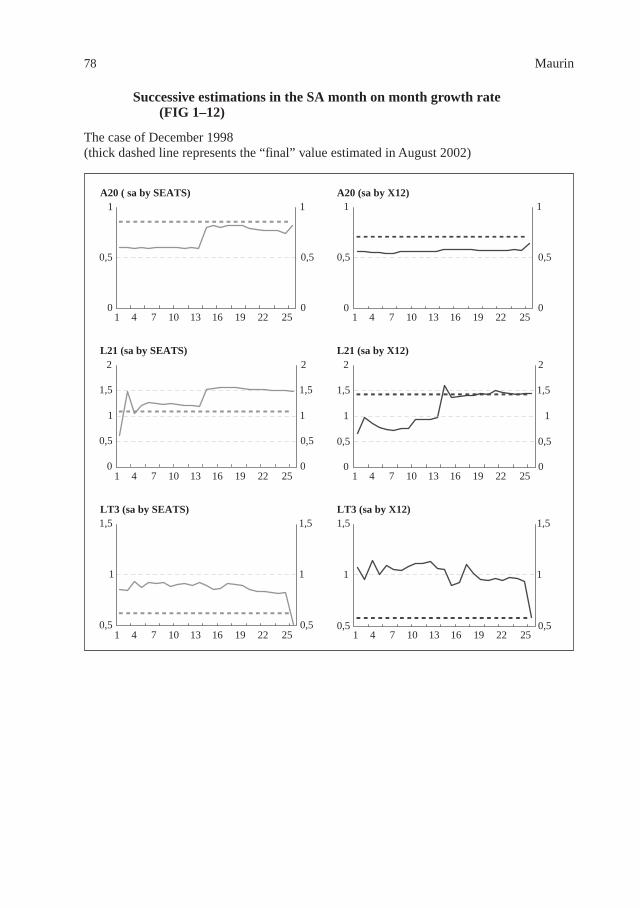
78 Maurin
Successive estimations in the SA month on month growth rate(FIG 1–12)
The case of December 1998(thick dashed line represents the “final” value estimated in August 2002)
A20 ( sa by SEATS) A20 (sa by X12)
L21 (sa by SEATS) L21 (sa by X12)
LT3 (sa by SEATS) LT3 (sa by X12)
0
0,5
1
0
0,5
1
0
0,5
1
1 4 7 10 13 16 19 22 25 1 4 7 10 13 16 19 22 25
1 4 7 10 13 16 19 22 25 1 4 7 10 13 16 19 22 25
1 4 7 10 13 16 19 22 25 1 4 7 10 13 16 19 22 250,5
1
1,5
0,5
1
1,5
0
0,5
1
1,5
2
0,5
1
1,5
0
0,5
1
1,5
2
0
0,5
1
1,5
2
0
0,5
1
0,5
1
1,5
0
0,5
1
1,5
2

Criteria to determine the optimal revision policy 79
M10 (sa by SEATS) M10 (sa by X12)
M20 (sa by SEATS) M20 (sa by X12)
M30 (sa by SEATS) M30 (sa by X12)
0
0,5
1
1,5
0
0,5
1
1,5
0
0,5
1
1,5
0
0,5
1
1,5
0 0
0,5
1
1,5
0,5
1
1,5
-0,5
0
0,5
-0,5
0
0,5
-0,5
0
0,5
0
0,5
1
1,5
0
0,5
1
1,5
-0,5
0
0,5
1 4 7 10 13 16 19 22 25 1 4 7 10 13 16 19 22 25
1 4 7 10 13 16 19 22 25 1 4 7 10 13 16 19 22 25
1 4 7 10 13 16 19 22 25 1 4 7 10 13 16 19 22 25
Successive estimations in the SA month on month growth rate(FIG 1–12)
The case of December 1998(thick dashed line represents the “final” value estimated in August 2002)

80 Maurin
Successive estimations in the SA month on month growth rate(FIG 13–24)
The case of March 1999(thick dashed line represents the “final” value estimated in August 2002)
A20 (sa by SEATS) A20 (sa by X12)
L21 (sa by SEATS) L21 (sa by X12)
LT3 (sa by SEATS) LT3 (sa by X12)
0
0,5
1
0
0,5
1
-1
-0,5
0
-1
-0,5
0
0
0,5
1
1,5
0
0,5
1
1,5
0
0,5
1
0
0,5
1
-1
-0,5
0
-1
-0,5
0
0
0,5
1
1,5
0
0,5
1
1,5
1 4 7 10 13 16 19 1 4 7 10 13 16 19
1 4 7 10 13 16 19 1 4 7 10 13 16 19
1 4 7 10 13 16 19 1 4 7 10 13 16 19

Criteria to determine the optimal revision policy 81
Successive estimations in the SA month on month growth rate(FIG 13–24)
The case of March 1999(thick dashed line represents the “final” value estimated in August 2002)
M10 (sa by SEATS) M10 (sa by X12)
M20 (sa by SEATS) M20 (sa by X12)
M30 (sa by SEATS) M30 (sa by X12)
0,5
1
1,5
0,5
1
1,5
0
0,5
1
0
0,5
1
0,5
1
00
0,5
1
0,5
1
1,5
0,5
1
1,5
0
0,5
1
0
0,5
1
0,5
1
00
0,5
1
1 4 7 10 13 16 19 1 4 7 10 13 16 19
1 4 7 10 13 16 19 1 4 7 10 13 16 19
1 4 7 10 13 16 19 1 4 7 10 13 16 19

82 Maurin
Comparing the sequences
Summary Tables 3 to 9
A20: Revisions on seasonal factors
SEQ Using SEATS Using X12TAR MAR RMSR d75 d90 mc sc TAR MAR RMSR d75 d90 mc sc
1 8 4 9 12 0,23 0,30 8 2 5 0,24 0,312 8 3 9 11 0,25 0,35 8 5 11 0,18 0,213 8 3 8 10 13 0,26 0,37 8 3 7 0,20 0,244 10 4 11 12 13 0,25 0,335 9 3 8 11 0,25 0,34 8 3 8 0,25 0,336 9 3 8 11 12 0,26 0,37 8 4 9 0,20 0,267 8 3 9 11 12 0,26 0,37 8 3 8 0,20 0,238 11 3 10 10 12 0,29 0,409 11 3 10 11 0,28 0,39
10 11 3 11 0,32 0,4411 10 4 11 9 0,29 0,39 8 3 8 0,25 0,3312 10 3 10 10 12 0,30 0,41 8 3 8 0,23 0,3213 10 3 11 10 12 0,29 0,40 8 3 7 0,22 0,2914 10 3 10 9 0,30 0,42 8 2 6 0,22 0,2615 11 3 11 9 11 0,30 0,4216 11 3 11 10 12 0,30 0,4217 11 4 12 12 0,27 0,3718 11 3 11 0,32 0,4419 11 3 11 0,31 0,4220 12 3 12 0,34 0,42
Results aggregated across time (Dec. 1998 to Nov. 1999)
L21: Revisions on seasonal factors
SEQ Using SEATS Using X12TAR MAR RMSR d75 d90 mc sc TAR MAR RMSR d75 d90 mc sc
1 37 16 37 9 11 0,25 0,32 29 7 20 10 12 0,25 0,322 32 20 46 9 10 0,25 0,33 25 27 50 0,16 0,183 33 11 37 9 10 0,27 0,37 31 18 31 11 0,17 0,204 43 14 55 0,30 0,395 30 13 34 10 11 0,25 0,34 22 11 31 0,25 0,306 31 11 39 10 10 0,28 0,39 29 18 40 0,19 0,257 32 11 39 10 10 0,28 0,40 29 15 34 12 0,20 0,228 42 13 45 0,29 0,409 43 13 48 0,29 0,40
10 42 12 47 0,33 0,4711 27 11 44 10 11 0,31 0,44 22 11 31 0,25 0,3012 27 11 44 10 11 0,31 0,44 27 12 31 0,23 0,3013 27 10 44 10 11 0,31 0,44 28 12 32 0,23 0,3014 27 10 44 10 11 0,31 0,45 28 8 21 0,21 0,2415 42 13 46 0,30 0,4416 42 12 46 0,30 0,4417 42 13 47 0,30 0,4318 42 12 47 0,33 0,4719 42 12 47 0,33 0,4720 43 12 56 0,35 0,47
Results aggregated across time (Dec. 1998 to Nov. 1999)

Criteria to determine the optimal revision policy 83
LT3: Revisions on seasonal factors
SEQ Using SEATS Using X12TAR MAR RMSR d75 d90 mc sc TAR MAR RMSR d75 d90 mc sc
1 27 7 18 0,25 0,33 34 14 32 0,21 0,252 28 6 17 0,26 0,36 41 18 38 0,18 0,203 27 7 18 0,25 0,33 41 18 38 0,18 0,204 39 8 28 0,32 0,415 30 5 16 0,26 0,35 40 12 31 0,22 0,256 28 7 19 0,25 0,33 37 15 36 0,19 0,217 27 6 18 0,25 0,33 40 12 31 0,22 0,258 42 6 27 0,36 0,479 38 6 25 0,35 0,45
10 37 5 27 0,36 0,4811 30 5 16 0,26 0,35 40 12 31 0,22 0,2512 28 7 18 0,25 0,33 38 17 38 0,18 0,1913 27 6 18 0,25 0,33 36 13 33 0,23 0,2614 27 7 18 0,25 0,33 40 12 31 0,22 0,2515 41 6 26 0,36 0,4716 38 6 25 0,35 0,4517 38 6 25 0,35 0,4518 37 5 27 0,36 0,4819 37 5 27 0,36 0,4820 36 5 27 0,36 0,47
Results aggregated across time (Dec. 1998 to Nov. 1999)
M10: Revisions on seasonal factors
SEQ Using SEATS Using X12TAR MAR RMSR d75 d90 mc sc TAR MAR RMSR d75 d90 mc sc
1 54 19 48 10 11 0,23 0,30 18 6 18 12 13 0,23 0,282 31 23 63 9 10 0,24 0,33 16 31 58 0,17 0,203 31 23 63 9 10 0,24 0,33 18 9 21 12 0,22 0,274 49 29 82 0,26 0,345 30 16 50 9 11 0,27 0,37 16 13 38 0,24 0,306 33 29 64 8 10 0,23 0,30 18 19 43 13 0,20 0,277 30 16 50 9 11 0,27 0,37 18 12 30 13 0,21 0,258 49 20 63 8 0,28 0,389 49 20 63 8 0,28 0,38
10 43 11 40 0,33 0,4511 20 8 28 11 0,30 0,42 16 13 38 0,24 0,3012 27 37 69 9 10 0,20 0,23 17 13 35 0,22 0,2913 26 14 43 10 11 0,26 0,36 16 12 33 0,23 0,2914 20 8 28 11 0,30 0,42 18 6 16 12 0,24 0,3115 43 11 39 0,31 0,4316 48 18 55 8 0,28 0,3817 43 11 39 0,31 0,4318 43 11 40 0,33 0,4519 43 11 40 0,33 0,4520 45 10 48 0,35 0,46
Results aggregated across time (Dec. 1998 to Nov. 1999)
Summary Tables: comparing the sequences

84 Maurin
Summary Tables: comparing the sequences
M20: Revisions on seasonal factors
SEQ Using SEATS Using X12TAR MAR RMSR d75 d90 mc sc TAR MAR RMSR d75 d90 mc sc
1 19 6 13 10 0,21 0,25 12 3 8 12 0,26 0,332 12 6 16 8 0,24 0,29 15 12 22 8 0,19 0,213 13 6 17 8 0,24 0,31 14 6 11 0,19 0,244 15 9 25 0,28 0,355 12 5 16 7 0,27 0,35 16 5 13 9 0,24 0,296 12 5 16 7 0,27 0,36 14 7 16 10 0,22 0,297 12 5 16 8 0,28 0,37 14 6 13 12 0,21 0,278 14 6 19 0,30 0,409 14 6 19 0,32 0,42
10 12 5 17 0,30 0,4311 7 4 15 9 0,29 0,38 16 5 13 9 0,24 0,2912 7 4 15 9 0,28 0,39 15 5 13 10 0,24 0,3213 7 4 14 10 0,28 0,39 16 5 14 10 0,24 0,3114 7 4 15 10 0,28 0,39 14 4 9 0,23 0,3015 13 5 16 0,27 0,3816 13 5 15 0,29 0,4017 13 6 17 0,24 0,3418 12 5 17 0,30 0,4319 12 5 16 0,29 0,4120 13 5 19 0,34 0,46
Results aggregated across time (Dec. 1998 to Nov. 1999)
M30: Revisions on seasonal factors
SEQ Using SEATS Using X12TAR MAR RMSR d75 d90 mc sc TAR MAR RMSR d75 d90 mc sc
1 15 4 10 9 11 0,28 0,38 13 3 8 12 13 0,27 0,372 15 4 11 9 11 0,29 0,39 13 9 17 12 0,17 0,193 11 4 13 9 9 0,29 0,40 13 4 9 13 0,23 0,304 20 6 25 5 0,32 0,415 15 2 7 10 11 0,30 0,42 12 4 12 0,25 0,306 11 3 9 9 11 0,29 0,40 11 7 14 12 0,19 0,257 10 3 9 9 12 0,29 0,42 13 4 11 0,22 0,258 13 4 16 7 0,34 0,469 13 4 14 7 0,32 0,44
10 13 4 16 0,35 0,4911 15 2 7 10 11 0,30 0,42 12 4 12 0,25 0,3012 11 3 9 9 11 0,29 0,40 12 5 11 0,23 0,3113 10 3 9 9 12 0,29 0,42 13 4 11 11 0,24 0,3314 9 3 9 0,28 0,40 13 3 8 0,25 0,3215 13 4 16 7 0,34 0,4616 13 4 14 7 0,32 0,4417 11 6 15 9 0,27 0,3818 13 4 16 0,35 0,4919 13 4 14 0,33 0,4320 11 3 16 0,35 0,45
Results aggregated across time (Dec. 1998 to Nov. 1999)

5
Direct versus indirect seasonal adjustment of UK monetarystatistics: preliminary discussion
David Willoughby
Historical background
The United Kingdom’s monetary statistics were traditionally analysed in a flow of fundscontext, with movements in the money stock being considered in conjunction with those inthe “counterparts”, such as credit to the private sector, public sector, and external influences.For each period, transactions were assembled in the form of a matrix arranged by financialinstrument and by economic sector. A flow in one cell of the matrix had to be offset by equaland opposite flows elsewhere, so that the matrix “balanced”. If the flow of funds matrix wasto be adjusted by subtracting seasonal variations, then it was reasonable to expect that theadjusted matrix should continue to be balanced. It followed, therefore, that an essentialproperty of the seasonal adjustment method was that it must produce a balanced set ofseasonal adjustments for the matrix.
Before 1990, the seasonal adjustments were generated using a two-stage method. The firststage involved using conventional univariate procedures in the sense that they derived theseasonal adjustments for a series without reference to other series in the matrix, so that theresulting seasonal matrix for each period did not balance. The second stage involvedamending the univariate adjustments so that they did balance. It was hoped that by exploitingthe information inherent in the accounting relationship between the series, the balancingprocess would demonstrably improve the seasonal adjustments. In practice, however, thebalanced seasonal adjustments were never entirely satisfactory. Although the univariateprocedures generally produced plausible results, it proved to be difficult to allocate the largeresulting imbalances across the series in an acceptable way. In some cases the balancingamendments proved to be so large that, when the balanced seasonal adjustments wereapplied, an apparently seasonal pattern remained, albeit of a different form to that present inthe unadjusted series.
By the late 1980s, users of the seasonally adjusted monetary data began to question thegrowing complexity, and frequent changes, of the methodology. The judgement involvedmade the method very resource intensive, especially when applied to the roughly 650 seriesthat were adjusted at the time. The bulk of the work had to be undertaken by specialists, whichpresented an obstacle to automation of the method. Automation was essential to allow currentupdating to be implemented at a reasonable cost. (Current updating had been recommendedby an independent Working Party.) In 1989, therefore, the Bank of England decided toundertake a fundamental reform of its seasonal adjustment work, with the aim of producing asimplified one-stage procedure that would produce inherently balanced adjustments, with aminimal need for judgmental intervention.
The solution to the balancing problem was to apply a common, linear seasonal adjustmentprocedure to every cell in the flow of funds matrix. The procedure was linear in the sense that,at any particular point in the series, the seasonal adjustment was a weighted additive or linearcombination of nearby observations. The package was developed within the Bank, and

86 Willoughby
named General Linear Abstraction of Seasonality (GLAS). It was acknowledged that it couldbe seen as very restrictive to require that the seasonal adjustment procedure be linear, and toapply the same procedure, with fixed filtering properties, to every series in the matrix. On theother hand, the subjective nature of seasonality meant that, provided the common filter itselfwas well designed, the method would produce satisfactory results.
The linear properties of GLAS ruled out several options often provided by seasonaladjustment procedures, including:• Adjustable smoothing• Non-seasonal series• Multiplicative seasonal models• Automatic outlier modification• Systematic identification and removal of calendar effects (for differing lengths of months,
public holidays, etc.).However, in the context of seasonally adjusting a flow of funds matrix, the cost was seen as
tolerably small. Furthermore, in the case of dealing with outliers in the data, the manualapproach that was used, which involved investigating the causes and locating the offsettingmovement, was fully consistent with trying to understand the movements in the underlyingdata.
GLAS has performed well in terms of the remit it had been given, ie the balancingconstraint, ease of use and resource efficiency. The pressure for change can be traced back toa workshop held at the Bank in March 2000, where there was general agreement that the Bankhad fallen behind the mainstream in its approach. GLAS had been written to honouradditivity, but the lack of diagnostics meant that users did not know the price they werepaying for this feature. In addition to the views expressed at the workshop, at this time thepolicy use of the data had also changed, with the focus increasingly on the (by then monthly)sectoral breakdowns of broad money and credit. Although this move to a sectoral approachdid not mean that the question of balancing had gone away, the lower profile of thecounterparts to broad money certainly made the consideration of alternative approaches toseasonal adjustment more viable.
Project to switch to X-12-ARIMA
Earlier reviews of seasonal adjustment methodology in the Bank of England have tended toget side-tracked by detailed comparisons of the outputs from various packages. Experience ofother central banks and national statistical institutions identified X-12-ARIMA and TRAMO-SEATS as the most viable options to replace GLAS. We favoured X-12-ARIMA partlybecause it is the methodology used by the Office for National Statistics, which would meanthat UK data were adjusted using consistent methodology. In addition, thework taking place to incorporate some of the modelling capabilities of TRAMO-SEATS intoX-12-ARIMA, the excellent diagnostics of X-12-ARIMA, and the documentation andsupport provided by the US Census Bureau, would meet the aims of the Bank of England inmoving to international best practice.
As noted above, a key feature of GLAS is that it generates seasonally adjusted data thatobey the same accounting constraints as the unadjusted data. Consequently, the issue of directversus indirect adjustment has not arisen, since both approaches generate the same outcome.So switching to X-12-ARIMA entails deciding whether to adopt a direct or indirect approachto the seasonal adjustment of the key monetary series. In the context of broad money and itscomponents, the indirect approach would be where seasonally adjusted M4 was compiled as

Direct versus indirect seasonal adjustment of UK monetary statistics 87
the sum of its seasonally adjusted components. (Indirect adjustment is generally consideredbetter when the component series have distinct seasonal patterns, and direct adjustment whenthe component series have similar seasonal patterns.)
The ECB’s paper of August 2000 set out the issues weighing on the question of directversus indirect adjustment of M3. Although no clear “winner” could be found, the decision touse an indirect method of adjustment was, in part, based on the practical consideration ofensuring the addivity of the seasonally adjusted components to the seasonally adjustedaggregate.
The paper also noted that the issue of addivity had two dimensions, ie not only thecomponents but also the balance sheet counterparts. The relatively short run of data meansthat the ECB has not yet had to address the issue of seasonal adjustment of the counterparts.But this is an issue for the Bank of England. And there is also a third dimension representedby the sectoral breakdowns of broad money and credit, where there is sufficient monthly datato be able to seasonally adjust, as well as longer runs of quarterly data.
The Bank of England’s experience in using the sectoral breakdowns of broad money andcredit was noted in the discussions leading up to the adoption of Regulation ECB/2001/13.The latter will furnish the ECB with similar data on a monthly basis to those which have beenavailable to the Bank of England since 1997. In due course, when a sufficiently long run ofthese new sectoral data are available, the ECB is likely to face a similar question to thatcurrently being addressed in the Bank, namely whether broad money and aggregate credit tothe private sector should be seasonally adjusted directly, or indirectly as the sum of theseasonally adjusted sectoral components. Some preliminary results from the seasonaladjustment of the UK quarterly sectoral data using X-12-ARIMA are presented below.
Preliminary results from the adjustment of sectoral data
The preliminary analysis of the seasonal adjustment of the sectoral components of broadmoney and private sector credit have been carried out using the quarterly data which areavailable back to 1963. The series were prior adjusted for breaks, and then analysed withX-12-ARIMA using the standard options (multiplicative, automatic ARIMA modelling, oneyear’s forecast appended, automatic scan for AO and LS outliers). To give an easy direct-indirect comparison, the composite spec was used; this automatically calculates the statisticsfor the indirect route and compares them with the direct analysis.
Looking first at broad money (M4) and its sectoral component series, “Automdl” found amodel with little difficulty in each case, usually either (0 1 1)(0 1 1) or (0 1 2)(0 1 1), and thediagnostics were satisfactory. Usually no AO or LS outliers were found. All series hadidentifiable seasonality and a satisfactory Q statistic for overall adequacy of adjustment. Allhad some M statistics outside limits, usually M8, M10 or M11 indicating moving seasonalityor M4 indicating autocorrelated irregulars.
The composite analysis showed satisfactory diagnostics for the indirect analysis. TheQ value was exactly the same as for the direct (0.42), though a different M was outside thelimits (M8 instead of M4). The “roughness statistics” which show which series is smootherindicate that direct is slightly smoother over the whole series but indirect over the last threeyears. It is confirmed that indirect has no residual seasonality, either over the whole series orthe recent years. Chart 1 compares quarterly growth rates of M4 since 1996 derived fromdirect and indirect adjustment; non-seasonally-adjusted rates are also included.
Aggregate private sector credit (M4 lending) has also been analysed. This analysis had afew complications in the modelling, and there were more level shifts in the early years than

88 Willoughby
with M4, but nothing to give any concern about interpretation of the results. The comparisonof direct and indirect via the X-12 M and Q statistics showed essentially the same result(Q=0.40 direct, Q=0.41 indirect, only M8 just outside limits in each case). Chart 2 comparesthe quarterly growth rates.
Chart 2: Comparison of quarterly M4 lending growth(percent)
-1
0
1
2
3
4
5
-1
0
1
2
3
4
5
directindirectn.s.a.
1996 1997 1998 1999 2000 2001 2002 2003
Chart 1: Comparison of quarterly M4 growth(percent)
5
4
3
2
1
0
-1
5
4
3
2
1
0
-11996 1997 1998 1999 2000 2001 2002 2003
directindirectn.s.a.

Direct versus indirect seasonal adjustment of UK monetary statistics 89
Some qualifications
Although these preliminary results show little difference between the indirect and directadjustment of broad money and private sector credit, there are some important qualifications.Firstly, even if M4 and M4 lending are seasonally adjusted indirectly as the sum of theseasonally adjusted sectoral component series, the issue of additivity still remains. This isbecause both aggregates can be broken down in alternative ways – see Charts 3 and 4. Forexample, in Chart 3, if M4 is seasonally adjusted indirectly as the sum of its sectoralcomponents, it is unlikely that the sum of its retail and wholesale elements will produce thesame result. Policy use of the data would dictate that the sectoral breakdown should takeprecedence, but the question of the lack of additivity remains as far as the retail/wholesalesplit is concerned.
The second qualification is that individual sector series have themselves been adjusteddirectly. It is possible that the quality of the seasonal adjustment could be improved if thesesectoral series were themselves adjusted indirectly, by summing their seasonally adjustedcomponents. If so, this might change the comparison between the direct/indirect adjustmentof M4 and M4 lending.
Chart 3: M4 coloured (greyed out) boxes currently seasonally adjusted
PNFCholdings of
Notes and Coin
Bankdeposits from
PNFCs
BuildingSociety
deposits fromPNFCs
Bankdesposits from
households
Householdholdings of
Notes
BuildingSociety
deposits fromhouseholds
OFCholdings of
Notes and Coin
Bankdeposits from
OFCs
BuildingSociety
deposits fromOFCs
HouseholdsDeposits with
MFIs plus notes
Householdsholdingof Coin
PNFCDeposits with
MFIs plus notes
PNFC holdingof Coin
OFCDeposits with
MFIs plus notes
OFC holding of Coin
Bankwholesaledeposits
BuildingSociety
wholesaledeposits
Total issuesof Coin
Private sectorholdings of
notes
MFI retaildeposits
excludingnotes
Bank retaildeposits
BuildingSocietyretail
deposits
Banks interestbearingdeposits
Banks non-interestbearingdeposits
Households
PNFC
OFC
M4
Retail
Wholesale

90 Willoughby
Third, and more significantly, in the case of at least one of the sectoral series (lending to thehousehold sector – see Chart 4) many of the sub-component series are highly policy-sensitiveand therefore require optimum seasonal adjustment. So even if the issue of direct versusindirect adjustment does not arise at the aggregate level (in the sense that the indirectadjustment of M4 and M4 lending is acceptable) there may still be problems lower down thepyramid.
Chart 4: M4 Lending coloured (greyed out) boxes currently seasonally adjusted
Bank netcredit card
lending
Bank netother unsec
lending
Bank netunsecured
lending
Bank netsecuredlending
Banklending toindividuals
Banklending to un-incorporatedbusinesses
Bsoc netcredit card
lending
Bsoc netother unsec
lending
Bsoc netunsecured
lending
Bsoc netsecuredlending
Bsoclending toindividuals
Bsoclending to un-incorporated
Bankslending to
Households
Bankslending to
PNFCs
Bsoclending to
PNFCs
Bsocslending to
OFCs
Bankslending to
OFCs
Bsocslending to
Households
MFIlending to
OFCs
MFIlending to
Households
MFIlending to
PNFCsM4L
Banklending toM4 sector
Bsoclending toM4 sector
Banks loansto M4 sector
M4 sectorsecuritiesheld byBanks
Bsocs loansto M4 sector
M4 sectorsecuritiesheld byBsocs
Bank netcredit card
lending
Bsoc netcredit card
lending
Bank netother unsec
lending
Bsoc netother unsec
lending
MFIconsumer
creditlending
MFIsecuredlending
MFIlending to
unin-corporatedbusinesses
andNPISH
Bank netsecuredlending
Bsoc netsecuredlending
Banklendingto unin-
corporatedand NPISH
Bsoc lend tounin-
corporatedand NPISH
MFI netcredit card
lending
MFI netother
unsecuredlending
Bankstats table 4.4 approach to households

6
The seasonal adjustment of euro area monetary aggregates:direct versus indirect approach
Romana Peronaci
1 Introduction
The seasonal adjustment of euro area monetary aggregates, M1, M2 and M3 can be obtainedindirectly through the aggregation of the main components previously seasonally adjusted ordirectly seasonally adjusting the aggregated series. The current procedure followed by theEuropean Central Bank (ECB) for the derivation of the monetary aggregates M2 and M3 isbased on the indirect seasonal adjustment. According to this, M2 is derived by aggregatingthe seasonally adjusted components M1 and the “Other short term deposits” (M2-M1), andM3 is finally obtained by adding to them the “Marketable instruments” (M3-M2).1
Empirical results show that the direct and the indirect seasonal adjustment of the same timeseries, produce same results only under very restrictive assumptions, that is when no tradingday or outlier adjustment is made, when the seasonal decomposition is additive, and when noforecast is produced. However the discrepancies in the seasonally adjusted series obtainedwith the two methods might not be necessarily significant.
In this paper we compare the results obtained from the direct and the indirect seasonaladjustment of the monetary aggregates M2 and M3, using the X12-Arima diagnostics toevaluate the quality of the two seasonal adjustments and the differences between the twoadjustments. The analysis is performed on the notional stocks2 in order to ensure theadditivity of the main components of the two aggregated series M2 and M3 as required byX12-Arima.
The work is organised as follows: Section 2 provides a description of the common criteriaand diagnostics used to assess the quality of a seasonal adjustment and to compare seasonaladjustment results obtained with the alternative approaches. Section 3 reports the results ofthe direct and the indirect seasonal adjustment of M2 and M3 on the basis of these criteria.Section 4 reports the conclusions.
2 Seasonal adjustment: direct versus indirect approach
One of the recommendations of the ECB Task Force on Seasonal Adjustment held in 1999,was the use of the indirect approach for the seasonal adjustment of the euro area monetaryaggregates. The choice was supported by practical considerations, by some criteria
1 “Seasonal adjustment of monetary aggregates and HICP for the euro area”, (August 2000), EuropeanCentral Bank.
2 The notional stocks are derived on the basis of the end-month stocks adjusted for the monthly changesnot due to financial transactions. The ECB official seasonal adjustment of monetary aggregates is performedon the index of notional stocks (see details in ECB (2000)).

92 Peronaci
identifying the “preferred” characteristics of the seasonal adjustment, like the minimisation ofrevision errors and the out of sample forecast accuracy, and also by the conclusions of deeperinvestigations of the series concerned in terms of their seasonal and cyclical components andtheir relative importance within the aggregate series.
After three years since the implementation of seasonal adjustment procedures at the ECB,the need to re-assess the quality of the indirect adjustment versus the direct adjustment hasarisen. Some empirical works have touched this aspect in the recent years, in particular withrespect to the seasonal adjustment of euro area GDP (Astolfi, Ladiray and Mazzi (2001)), andeuro area HICP (Cristadoro and Sabbatini (2000)). Other recent works developed statisticaltests to compare the results obtained by the indirect and the direct approach and to assesswhich one performs better, as Planas and Campolongo (2000), Gomez (2000), Otranto andTriacca (2000). On the basis of these works a set of empirical criteria has been identified andis used here to evaluate the performance of the direct and indirect adjustment for the euro areamonetary aggregates series M2 and M3. The criteria are described below.
a) Graphical analysis and sign concordance
In principle the two approaches to derive seasonally adjusted (SA) series of the euro areamonetary aggregates should lead to similar results, and the growth rates of the SA seriesshould have the same sign. This is an essential aspect to be assessed in order to be able todeliver reliable statistical information to the users and to the public in general. In particularthis is a critical issue for what concerns the seasonal adjustment of the euro area monetaryaggregates, since these statistics are regularly used by the ECB to monitor the monetarysituation of the euro area and to define its monetary policy.
For this purpose, a preliminary investigation of the results obtained with the direct and withthe indirect approach is performed through the graphical analysis of the SA series obtainedfrom the two approaches. In addition to this, the inspection of the SA annual growth ratesseries allows verification of whether the two approaches lead to a similar detection of turningpoints in the SA series. A further step concerns the consistency between the growth rates ofthe SA aggregated series and their adjusted components, which should evolve in the samedirection. Hence, two statistics are used to assess the degree of consistency in the growthrates, which are calculated on the basis of the ratio of growth rate values, for the sameobservations, showing similar sign. The first statistics, C1, measures the percentage ofconcordance between the direct and indirect series and the second, C2, the percentage ofconcordance between the SA aggregate and the SA components.
b) Analysis of smoothness
One of the aspects taken into consideration in the choice between direct and indirect seasonaladjustment is the roughness of the SA series. Dagum (1979) proposed two measures ofroughness or lack of smoothness, of the SA series, that measure the size of their deviationsfrom a smooth trend, and are based on the first difference filter and on the 13-term Hendersonfilter applied to the SA series.
The first measure is defined as:
where {At : 1� t � N} is the adjusted series and is the length of the series.
( )N
AAN
RN
t tt
2
211
1
1
1
1
= − ×−
=−×−
=N
t 2=( )A
t
2
∇

The seasonal adjustment of euro area monetary aggregates 93
The second measure is defined by:
where {At : 1� t � N} is the adjusted series and {H13At : 1� t � N} is the output from a 13-termHenderson filter that is applied to it.
c) Residual seasonality in the adjusted series
Generally, the quality of a seasonal adjustment is assessed on the basis of any significantresidual seasonality and calendar effects left in the SA series. The existence of residualseasonality in the SA series when this is obtained with the direct approach can result from aninadequate adjustment procedure, or from the existence of seasonality difficult to estimate inthe original series. A SA series obtained indirectly by aggregating the SA components, mightshow residual seasonality when the seasonal and trading day effects present in thecomponents series are not easily detectable and are not properly estimated, leaving residualeffects in the adjusted series.
The existence of residual seasonality or trading day effects in the SA series and in the SAcomponents is investigated here by means of the tests of residual seasonality proposed byX12-Arima and calculated on the SA series obtained with the direct and the indirectadjustment. Moreover, the analysis of the spectrum of the SA series allows detecting residualseasonality or residual trading day effects in the series (see Findley at al. (1998)).
d) Analysis of the irregular components
As next step in the investigation of residual seasonality after the direct and the indirectadjustment approaches are applied, we analysed the irregular components of the SA series(i.e. the detrended seasonally adjusted series). The estimated residual components, whichrepresent the irregular part of the series and are by definition white noise processes with zeroexpectation, non-correlated and of constant variance σ2, should not present any residualseasonality and trading day effects.
Firstly, to assess the existence of seasonal or trading day effects in the residual component,the spectrum of the final irregular component for the direct and the indirect adjustment areinvestigated. Then a set of test statistics is calculated for the irregular components of the twoaggregated series to test for their randomness and absence of first order autocorrelation.
e) Quality of seasonal adjustment
X12-Arima computes a set of eleven indicators to assess the quality of the seasonaladjustment. These indicators are purely descriptive and based on empirical criteria (seeQuenneville and Ladiray (2001)) and have not been derived in order to derive conclusions onthe relative performance of the direct and indirect seasonal adjustments. However they can becalculated for the two approaches in order to verify whether these lead to significantlydifferent results in terms of the quality of the adjustments (see J. Lothian and M. Morry(1978)).
( ) ([1
2
1132
1
1
1
1
==×
−=−×
−=
N
t
N
t ttN
AHAN
R ) ]213
−t
AH1

94 Peronaci
)(min
)(min)(max100
kS
kSkSS
tNk
tNktNkMaxt
t
tt
∈
∈∈ −×= ;
f) Analysis of stability based on revision histories (1)
A further aspect that is relevant for the production of a satisfactory seasonal adjustmentconcerns the amount and the size of revisions the SA data undergo, when they are recalculatedas additional values for the raw series become available. Obviously, different causes canproduce unstable seasonal adjustments, some of which are unavoidable, as the existence ofmoving seasonality in the raw series. However, the analysis of stability of the seasonaladjustment can also shed some light on the comparison between direct and indirect seasonaladjustment.
The analysis of revisions associated with continuous seasonal adjustment over a number ofyears is one of the stability diagnostics available in X12-Arima (see D. Findley et al. (1998)).The natural way to measure the size of revisions to SA data is the comparison between theearliest adjustment of a month’s datum, obtained when that month is the final month in theseries (t), and a later adjustment based on all future data available at the time of the analysis(T). The formula below shows how the revision is calculated in the case of a multiplicativeseasonal decomposition.
Rt = 100 ×
where {At|n : n = 1,...,T} is the SA series, At|t is the “concurrent” adjustment and At|T is the“final” adjustment of the month t observation, calculated at the end of the time series.
A revision history of the seasonal adjustment for a series At is obtained calculating Rt overa consecutive set of time points within the series. The analysis is applied here to both thedirect and indirect seasonal adjustments to identify which approach leads to more stableresults in terms of revisions of the adjusted data.
g) Analysis of stability based on the sliding spans (2)
The second type of stability diagnostic available in X12-Arima is based on the comparison ofthe seasonal adjustment calculated on four overlapping sub-spans of the series (Findley at al.(1990), Findley at al. (1998)). For each month that is common to at least two sub-spans, thedifference between the largest and the smallest seasonal adjustment obtained from thedifferent spans for the reference month is analysed. Excessive variability among suchestimates indicates unreliability.
The analysis is performed for the direct and for the indirect seasonal adjustment of M2 andM3 and the results obtained for the two approaches are compared on the basis of thefollowing two statistics, to assess which one gives a more stable seasonal adjustment:
Max percent difference for seasonal factors:
where St (k) is the seasonal factor estimated from span k for month t.
Max difference formonthly changes in SA series:
where MMt(k) and At (k) is the SA value from span k for month t.
tt
ttTt
A
AA −
)(min)(max kMMkMMMM tNktNkMax
t tt ∈∈ −= ;
)(
)()(100
1
1
kA
kAkA
t
tt
−
−−×=

The seasonal adjustment of euro area monetary aggregates 95
3 The seasonal adjustment of euro area monetary aggregates
The direct and the indirect seasonal adjustment approaches are compared here on the basis ofthe results obtained for the seasonal adjustment of the euro area monetary aggregates M2 andM3. The euro area monetary aggregates M2 and M3 can be seasonally adjusted directly orindirectly as the sum of their SA components. In particular, M2 can be derived by aggregatingthe two components M1 and “other short term deposits” (M2-M1) previously seasonallyadjusted, while M3 can be derived by the aggregation of seasonally adjusted M1, M2-M1 and“Marketable instruments” (M3-M2).
Both direct and indirect approaches to the seasonal adjustment of the aggregated series M2and M3 were performed using X12-Arima3 on the end-month notional stocks series. The twoseries are seasonally adjusted according to the multiplicative decomposition.
a) Graphical analysis and sign concordance
Figure 1 reports the original series and the SA series according to the direct and the indirectapproaches for M2 and M3 for the period Aug92-Aug02. Figures 2 and 3 show the annualgrowth rates of the SA series derived with the two approaches.
As emerges from the graphical analysis no significant differences between the series,derived with the two approaches, can be identified. For what concerns the divergencebetween the growth rates series, this is clearly not significant as shown in Figure 4, with amaximum discrepancy between the seasonally adjusted annual growth rates series obtainedwith the two methods of 9 basis points and 18 basis points for M2 and M3 respectively, as alsoshown in Table 1.
3 X-12-ARIMA monthly seasonal adjustment Method, Release Version 0.2, U.S. Department ofCommerce, Bureau of the Census.
SeriesDiscrepancy between growth rates
C1 C2Average Standard deviation Max
M2 0.0001 0.0223 0.095 100% 100%M3 -0.0001 0.0404 0.180 100% 89.6%
Table 1: Direct versus indirect approach: comparison between the SA annualgrowth rates series
The annual growth rates derived on the basis of the direct and indirect SA series show fullsign concordance (100%) for the whole period for M2 and M3, as indicated by the results ofthe statistics C1 (percentage of concordance between the direct and indirect SA series). As forthe sign concordance between the growth rates of the SA components and the SA aggregateseries measured by C2 (percentage of concordance between the SA series and the SAcomponents), this is 100% for M2, while it is at around 90% for M3.

96 Peronaci
Figure 1: Original series, direct and indirect seasonally adjusted series ofM2 and M3(EUR billions)
2,500
3,000
3,500
4,000
4,500
5,000
5,500
6,000
2,500
3,000
3,500
4,000
4,500
5,000
5,500
6,000
1992 1993 1994 1995 1996 1997 1998 1999 2000 2001 2002
seasonally adjustedunadjusted
M3
M2
Figure 2: Annual growth rates of seasonally adjusted M2 obtained with thedirect and indirect approaches(percentage)
0.0
2.0
4.0
6.0
8.0
10.0
12.0
0.0
2.0
4.0
6.0
8.0
10.0
12.0
1981 1983 1985 1987 1989 1991 1993 1995 1997 1999 2001
direct approachindirect approach

The seasonal adjustment of euro area monetary aggregates 97
Figure 3: Annual growth rates of seasonally adjusted M3 obtained with thedirect and indirect approaches(percentage)
0.0
2.0
4.0
6.0
8.0
10.0
12.0
0.0
2.0
4.0
6.0
8.0
10.0
12.0
1981 1983 1985 1987 1989 1991 1993 1995 1997 1999 2001
direct approachindirect approach
Figure 4: Difference in the annual growth rates of seasonally adjusted M2and M3 obtained with the direct and indirect approaches (direct minusindirect adjustment)(percentage)
1981 1983 1985 1987 1989 1991 1993 1995 1997 1999 2001-0.20
-0.15
-0.10
-0.05
0.00
0.05
0.10
0.15
0.20
-0.20
-0.15
-0.10
-0.05
0.00
0.05
0.10
0.15
0.20
M2M3

98 Peronaci
b) Analysis of smoothness
The smoothness of the SA series derived with the two approaches is assessed using the twotests presented in par. 2/b and calculated for the whole series and for the last three years only,the results of which are presented in Table 2. On the basis of the two measures R1 and R2 noclear conclusion can be derived on which is the best approach in terms of smoothness of theSA series. As regards to both M2 and M3, the results obtained on the full series and on the lastthree years for R1 indicate that the direct adjustment is smoother than the indirect one. On theother hand, R2 gives opposite messages when calculated on the whole series and on the lastthree years only, showing a smoother indirect adjustment for M2 when applied to the lastthree years only and a smoother indirect adjustment for M3 when calculated on the wholeseries.
c) Residual seasonality in the adjusted series and in the irregularcomponents
The spectrum is normally estimated by X12-Arima for the most recent period of data, sinceusers are usually more concerned about recent data. However, in case of moving seasonalityand trading day effect, the results of the spectrum inspection limited to the most recent yearsmight be significantly different from those obtained on the whole series. For this reason, thespectrum is estimated first on the most recent eight years of data (as from September 1994 toAugust 2002) and then on the entire period available, for the two aggregates M2 and M3 andalso for their main components M1, M2-M1 and M3-M2.
The results of the spectrum inspection are reported in Table 3. Concerning the comparisonbetween the direct and indirect adjustment of M2 and M3, no residual seasonality or tradingeffects are found in the spectrum of the SA series and of the irregular components estimatedfor the whole period January 1980-August 2002 and for the most recent eight years period.
No residual seasonality is found for the component series M1, M2-M1 and M3-M2, forboth the whole period of data and for the most recent eight years. However the spectrum doesnot give a clear indication on the residual trading day effects left in the irregular component ofM1 and M3-M2.
Series Measures of Direct Indirect Percentage change1)
roughnessFull series Last 3 years Full series Last 3 years Full series Last 3 years
M2 R1 15611.28 20132.42 15759.00 20247.25 -0.953% -0.570%R2 0.002 0.001 0.002 0.001 -1.952% 0.533%
M3 R1 18044.31 26019.28 18271.27 26249.83 -1.258% -0.886%R2 0.002 0.001 0.002 0.001 5.096% -8.192%
Table 2: Measures of roughness for seasonally adjusted series:direct versus indirect approach
Notes: The root mean square errors of the tests are reported here.1) The percentage change values show the improvement in the smoothness of the SA series going from theindirect seasonal adjustment to the direct seasonal adjustment. A positive sign indicates that the indirectseasonal adjustment is smoother than the direct one.

The seasonal adjustment of euro area monetary aggregates 99
d) Further analysis of the irregular components
A further step in the analysis of the irregular components is testing for the randomness andthe absence of autocorrelation in these series. For this purpose, a set of test statistics is appliedto the irregular components of M2 and M3, the results of which are reported in Table 4.
The results of this analysis support the randomness of the irregular components obtainedfrom the two seasonal adjustment approaches, for both aggregates M2 and M3.
Test statisticsM2 M3
Direct SA Indirect SA Direct SA Indirect SA
Mean 1) 1 1 1 1Standard deviation 0.00103 0.00127 0.00098 0.00125Skewness 0.2766 0.1309 0.2008 0.1528Excess kurtosis 0.0220 -0.0160 0.0151 0.0382Asymptotic test [χ2
(2)] 2) 3.4749 [0.1760] 0.77122 [0.6800] 1.8297 [0.4006] 1.0750 [0.5842]
Normality test [χ2(2)
] 2) 3.6419 [0.1619] 0.81555 [0.6651] 1.8883 [0.3890] 1.1625 [0.5592]DW 3) 2.498 1.899 2.408 1.946ADF 4) -21.15** -15.59** -20.17** -15.96**
Notes: ** indicates a level of significance of 1%, * a level of significance of 5%.1) The mean of the irregular component obtained from the multiplicative adjustment in X12-Arima, iscentered to 1 by construction.2) The normality tests are a function of the skewness and excess kurtosis. In squared brackets is shown theprobability of getting a number at least as large if the series has a normal distribution.3) The Durbin Watson (DW) statistic is testing for whiteness against first order autocorrelation in the series. Ifthe series is white noise, DW will be around 2, if the series is a random walk (integrated of first order) DW willbe very small.4) A significant result for the Augmented Dickey Fuller test (ADF) indicates that the null hypothesis of a unitroot is rejected and the series is stationary. Critical values are derived from McKinnon (1991), two stars (**)indicate that the test is significant at the 1% level.
Table 4: Analysis of irregular components
Series Residual Direct Indirect Direct Indirecteffect
SA Irregular SA Irregular SA Irregular SA Irregularseries component series component series component series component
Sep. 1994 - Aug. 2002 Jan. 1980 - Aug. 2002
M2 Seasonality NO NO NO NO NO NO NO NOM2 Trading day NO NO NO NO NO NO NO NOM1 Seasonality NO NO NO NOM1 Trading day NO ? NO ?M2-M1 Seasonality NO NO NO NOM2-M1 Trading day NO NO NO NO
M3 Seasonality NO NO NO NO NO NO NO NOM3 Trading day NO NO NO NO NO NO NO NOM3-M2 Seasonality NO NO NO NOM3-M2 Trading day NO ? NO NO
Table 3: Spectrum analysis for seasonally adjusted series and irregular components
Notes: The spectrum are estimated by X12-Arima on the SA series modified for the extreme values identified byX11, and on the irregular component of the series modified for the extreme values identified by X11.

100 Peronaci
e) Quality assessment of seasonal adjustment
The results of the eleven quality measures (Ms) available in X12-Arima for the direct and the
indirect seasonal adjustment are reported in Table 5. The comparison between theperformance of the direct and the indirect approach for M2 and M3 does not show significantdifferences in terms of quality of the adjustment, with only one exception. For the indirectadjustment of M2 and M3 the value of the statistics M8 (1.428 and 1.562 respectively) areabove the acceptance value of 1 and significantly bigger than the value obtained for the directadjustment of M2 and M3 (0.454 and 0.489 respectively). However the statistics M8 and M10
for the indirect method give generally higher results than for the direct method, and they areconsidered crucial when they both show values above 1, as it is not the case here.
f) Analysis of stability using revisions histories
The analysis of lagged revisions consents to assess the behaviour of the revisions to theseasonal estimates over time. This is performed with respect to the concurrent seasonal
Seasonal adjustment quality indicators Index Notional stocks Index Notional stocks
M2 M2 M2 M3 M3 M3Direct Direct Indirect Direct Direct Indirect
Relative contribution of the irregularover three months span M
10.034 0.034 0.074 0.031 0.030 0.064
Relative contribution of the irregularcomponent to the stationary portion ofthe variance M
20.005 0.005 0.007 0.003 0.003 0.005
Amount of month to month changein the irregular component as comparedto the amount of month to month changein the trend-cycle M
30.000 0.000 0.000 0.000 0.000 0.000
Amount of autocorrelation in the irregularas described by the average duration of run M
40.560 0.560 0.784 0.952 0.840 1.400
Number of months it takes the change inthe trend-cycle to surpass the amount ofchange in the irregular M
50.000 0.000 0.000 0.000 0.000 0.000
Amount of year to year change in theirregular as compared to the amount ofyear to year change in the seasonal M
60.237 0.232 0.232 0.236 0.246 0.152
Amount of moving seasonality presentrelative to the amount of stable seasonality M
70.136 0.136 0.161 0.206 0.196 0.216
Size of the fluctuations in the seasonalcomponent throughout the whole series M
80.455 0.454 1.428 0.498 0.489 1.562
Average linear movement in the seasonalcomponent throughout the whole series M
90.199 0.199 0.209 0.300 0.291 0.291
Same as 8, calculated for recent years only M10
0.529 0.529 1.076 0.612 0.615 1.047
Same as 9, calculated for recent years only M11
0.492 0.493 0.680 0.592 0.597 0.696
Table 5: Direct versus indirect approach: seasonal adjustment quality indicators
Notes: These statistics vary between 0 and 3 and values below 1 are generally considered acceptable.

The seasonal adjustment of euro area monetary aggregates 101
adjustment (adjustment of observation t when this is the last observation available) and to thefinal seasonal adjustment (adjustment of month t calculated at the end of the time series). Inorder to evaluate the size of the revisions to the SA series when more observations are addedat the end of the period, the concurrent estimates are compared to the estimates obtained whenadditional observations become available, while to evaluate how quickly an estimateconverges to its final value, the final estimates are used as mean of comparison. Table 6 showsthe results of the analysis with respect to the concurrent seasonal adjustment (panel A) and tothe final seasonal adjustment (panel B).
For what concerns the size of the revisions to the SA data (Table 6 - A), no significantdifferences can be identified between the direct and the indirect seasonal adjustment for bothM2 and M3, with the exception of the revisions between the concurrent and the finaladjustment for M3, where the direct method seems to perform slightly better. When we lookat how quickly an estimate converges to its final value (Table 6 - B) the direct adjustmentshows a quicker convergence than the indirect adjustment for both M2 and M3.
Figure 6 and 7 show the concurrent and final adjustment for the direct and the indirectmethods for M2 and M3 respectively. The differences between the revisions obtained with thetwo methods (abs [R
tdirect]- abs [R
tindirect]) are also reported in the graphs with bars, where positive
values indicate larger revisions for the direct method and negative values indicate largerrevisions for the indirect method. The comparison between the concurrent and the finaladjustment of M3 (Figure 7) obtained with the two methods indicates a slightly betterperformance of the direct adjustment against the indirect one, even though in most of the casesthe discrepancies are quite small (below 5%). A similar result is obtained for M2 (Figure 6).
Additional M2 direct M2 indirect M3 direct M3 indirectobservations Mean Standard Mean Standard Mean Standard Mean Standard
deviation deviation deviation deviation
A. With respect to concurrent seasonal adjustment
1 extra month 0.05 0.026 0.05 0.019 0.04 0.020 0.05 0.0232 extra months 0.06 0.017 0.06 0.023 0.06 0.026 0.06 0.0223 extra months 0.07 0.013 0.07 0.023 0.06 0.024 0.07 0.0226 extra months 0.08 0.024 0.09 0.036 0.08 0.040 0.09 0.04112 extra months 0.10 0.028 0.11 0.038 0.12 0.040 0.12 0.043Final estimate 0.10 0.043 0.11 0.038 0.08 0.021 0.11 0.038
B. With respect to final seasonal adjustment
3 extra months 0.06 0.028 0.07 0.027 0.04 0.012 0.07 0.0236 extra months 0.07 0.028 0.08 0.026 0.05 0.017 0.08 0.01612 extra months 0.07 0.033 0.08 0.035 0.06 0.024 0.09 0.04018 extra months 0.03 0.019 0.05 0.020 0.03 0.020 0.06 0.01924 extra months 0.02 0.027 0.03 0.027 0.02 0.016 0.04 0.025
Table 6: Direct versus indirect approach: analysis of absolute revisions toseasonally adjusted data *(percentages)
* The size of revisions has been assessed over the 4-years-period from August 1999 to August 2002.(1) The size of the revisions is evaluated comparing the SA data obtained according to the concurrentadjustment with those obtained adding 1, 2, 3, 6 and 12 extra observations [Rt
= 100 × (At/t+lag-At/t)/At/t].(2) The size of the revisions is evaluated comparing the SA data obtained according to the final adjustmentwith those obtained adding 1, 2, 3, 6 and 12 extra observations after the current observation[Rt = 100 × (At/T-At/t+lag)/At/t+lag].

102 Peronaci
-0.25
-0.20
-0.15
-0.10
-0.05
0.00
0.05
0.10
0.15
0.20
0.25
-0.25
-0.20
-0.15
-0.10
-0.05
0.00
0.05
0.10
0.15
0.20
0.25
Aug. Nov. Feb. May Aug. Nov. Feb. May Aug. Nov. Feb. May
1999 2000 2001 2002
Indirect adjustmentDirect minus indirect adjustment
Direct adjustment
Figure 7: Revisions concurrent to final for the direct and indirect seasonal adjustmentof M3, and differences between the two approaches(percentage)
Figure 6: Revisions concurrent to final for the direct and indirect seasonal adjustmentvalues of M2, and differences between the two approaches(percentage)
-0.35
-0.30
-0.25
-0.20
-0.15
-0.10
-0.05
0.00
0.05
0.10
0.15
0.20
0.25
0.30
0.35
-0.35
-0.30
-0.25
-0.20
-0.15
-0.10
-0.05
0.00
0.05
0.10
0.15
0.20
0.25
0.30
0.35
Aug. Nov. Feb. May Aug. Nov. Feb. May Aug. Nov. Feb. May1999 2000 2001 2002
Indirect adjustmentDirect minus indirect adjustment
Direct adjustment
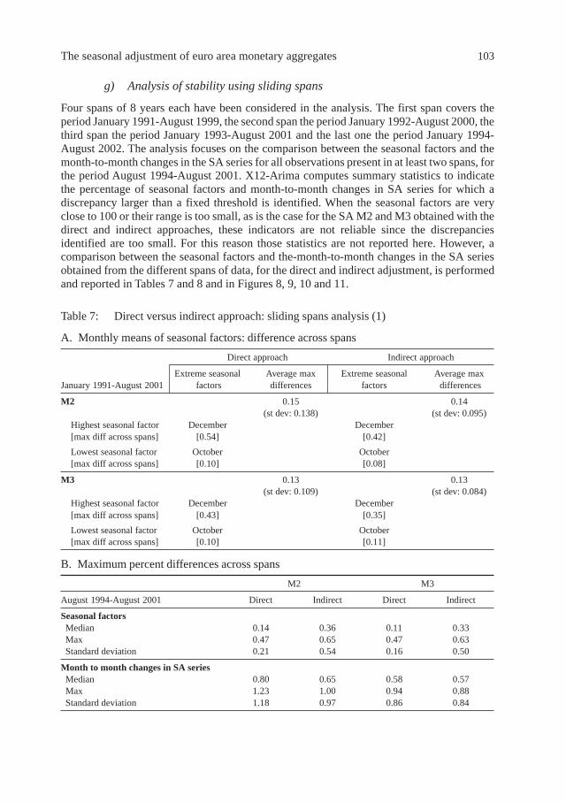
The seasonal adjustment of euro area monetary aggregates 103
g) Analysis of stability using sliding spans
Four spans of 8 years each have been considered in the analysis. The first span covers theperiod January 1991-August 1999, the second span the period January 1992-August 2000, thethird span the period January 1993-August 2001 and the last one the period January 1994-August 2002. The analysis focuses on the comparison between the seasonal factors and themonth-to-month changes in the SA series for all observations present in at least two spans, forthe period August 1994-August 2001. X12-Arima computes summary statistics to indicatethe percentage of seasonal factors and month-to-month changes in SA series for which adiscrepancy larger than a fixed threshold is identified. When the seasonal factors are veryclose to 100 or their range is too small, as is the case for the SA M2 and M3 obtained with thedirect and indirect approaches, these indicators are not reliable since the discrepanciesidentified are too small. For this reason those statistics are not reported here. However, acomparison between the seasonal factors and the-month-to-month changes in the SA seriesobtained from the different spans of data, for the direct and indirect adjustment, is performedand reported in Tables 7 and 8 and in Figures 8, 9, 10 and 11.
A. Monthly means of seasonal factors: difference across spans
Direct approach Indirect approach
Extreme seasonal Average max Extreme seasonal Average maxJanuary 1991-August 2001 factors differences factors differences
M2 0.15 0.14(st dev: 0.138) (st dev: 0.095)
Highest seasonal factor December December[max diff across spans] [0.54] [0.42]
Lowest seasonal factor October October[max diff across spans] [0.10] [0.08]
M3 0.13 0.13(st dev: 0.109) (st dev: 0.084)
Highest seasonal factor December December[max diff across spans] [0.43] [0.35]
Lowest seasonal factor October October[max diff across spans] [0.10] [0.11]
B. Maximum percent differences across spans
M2 M3
August 1994-August 2001 Direct Indirect Direct Indirect
Seasonal factorsMedian 0.14 0.36 0.11 0.33Max 0.47 0.65 0.47 0.63Standard deviation 0.21 0.54 0.16 0.50
Month to month changes in SA seriesMedian 0.80 0.65 0.58 0.57Max 1.23 1.00 0.94 0.88Standard deviation 1.18 0.97 0.86 0.84
Table 7: Direct versus indirect approach: sliding spans analysis (1)

104 Peronaci
First, we looked at the means of seasonal factors per month and at their discrepancies acrossthe spans, calculated over the complete four spans of data. No significant differences areidentified between the two approaches. The months of October and December are identifiedas having the lowest and the highest seasonal factors in all the data spans for both the directand indirect seasonal adjustment of M2 and M3 (Table 7A). Moreover, the seasonal factorsestimated with the direct method show slightly larger discrepancies as opposed to thoseestimated with the indirect method for these two extreme months.
Looking at the distribution of the largest discrepancies between the seasonal factors acrossthe spans for the 7-years period August 1994-August 2001, an indication of larger dis-crepancies and higher variability is evident in the indirect approaches for both M2 and M3(Table 7B), as also shown in Figure 8 and 9. However, this is not the case for the monthlypercentage changes calculated for the SA series of M2 in the different spans of data, where thepicture is the opposite, and the indirect approach is performing better in terms ofdiscrepancies across the different spans (Figure 10). As for the monthly percentage changescalculated on the SA M3 series, no significant differences between the direct and the indirectapproaches can be identified (Figure 11).
Finally, as shown in Table 8, the direct method performs better in terms of number ofmonths of inconsistent estimates of the seasonal factors across the spans for the two series,M2 and M3. However, the indirect method gives more stable results in terms of monthlypercentage changes across the spans for M2, while no differences are identified for M3.
Comparison between spans Direct approach Indirect approach
Number of Average Standard Number of Average Standardmonths dev months dev
Seasonal factorsM2 - Inconsistent estimates 1) 12 out of 84 17 out of 84
[14.3%] [20.2%]M2 - Max % difference 0.14 0.089 0.37 0.103M3 - Inconsistent estimates 1) 6 out of 84 15 out of 84
[7.1%] [18.9%]M3 - Max % difference 0.12 0.080 0.33 0.094
Month to month changes in SA seriesM2 - Sign inconsistency in 35 out of 84 30 out of 84monthly percentage changes 2) [40.5%] [35.7%]M2 - Max difference 0.74 0.280 0.60 0.218M3 - Sign inconsistency in 22 out of 84 23 out of 84monthly percentage changes 2) [26.2%] [27.4%]M3 - Max difference 0.54 0.224 0.53 0.189
Table 8: Direct versus indirect approach: sliding spans analysis (2)
1) Seasonal factors estimates are considered inconsistent when some are below 100 and some above 100,indicating an increase and a decrease in the SA value for the same observation across the spans.2) The monthly percentage changes calculated on the four spans show different signs.

The seasonal adjustment of euro area monetary aggregates 105
Figure 9: Largest percentage differences between seasonal factors across spansand inconsistent estimates – direct and indirect seasonal adjustment of M3
0.00
0.10
0.20
0.30
0.40
0.50
0.60
0.70
0.00
0.10
0.20
0.30
0.40
0.50
0.60
0.70
Aug. Nov. Feb. May Aug. Nov. Feb. May Aug. Nov. Feb. May Aug. Nov. Feb. May Aug. Nov. Feb. May Aug. Nov. Feb. May Aug. Aug.Nov. Feb. May
1994 1995 1996 1997 1998 1999 2000 2001
Indirect seasonal adjustment of M3Direct seasonal adjustment of M3Inconsistent estimates
Figure 8: Largest percentage differences between seasonal factors across spansand inconsistent estimates – direct and indirect seasonal adjustment of M2
0.00
0.10
0.20
0.30
0.40
0.50
0.60
0.70
0.00
0.10
0.20
0.30
0.40
0.50
0.60
0.70
Aug. Nov. Feb. May Aug. Nov. Feb. May Aug. Nov. Feb. May Aug. Nov. Feb. May Aug. Nov. Feb. May Aug. Nov. Feb. May Aug. Aug.Nov. Feb. May
1994 1995 1996 1997 1998 1999 2000 2001
Indirect seasonal adjustment of M2Direct seasonal adjustment of M2Inconsistent estimates

106 Peronaci
Figure 11: Largest differences between month to month changes across spansand sign inconsistencies – direct and indirect seasonal adjustment of M3(percentage)
Aug. Nov. Feb. May Aug. Nov. Feb. May Aug. Nov. Feb. May Aug. Nov. Feb. May Aug. Nov. Feb. May Aug. Nov. Feb. May Aug. Aug.Nov. Feb. May
1994 1995 1996 1997 1998 1999 2000 2001
0.00
0.10
0.20
0.30
0.40
0.50
0.60
0.70
0.80
0.90
1.00
0.00
0.10
0.20
0.30
0.40
0.50
0.60
0.70
0.80
0.90
1.00Indirect seasonal adjustment of M3Direct seasonal adjustment of M3Sign inconsistencies
Figure 10: Largest differences between month to month changes across spansand sign inconsistencies – direct and indirect seasonal adjustment of M2(percentage)
Aug. Nov. Feb. May Aug. Nov. Feb. May Aug. Nov. Feb. May Aug. Nov. Feb. May Aug. Nov. Feb. May Aug. Nov. Feb. May Aug. Aug.Nov. Feb. May
1994 1995 1996 1997 1998 1999 2000 2001
0.00
0.20
0.40
0.60
0.80
1.00
1.20
1.40
0.00
0.20
0.40
0.60
0.80
1.00
1.20
1.40Indirect seasonal adjustment of M2Direct seasonal adjustment of M2Sign inconsistencies

The seasonal adjustment of euro area monetary aggregates 107
4 Conclusions
In this paper we compared the performance of the direct and the indirect seasonal adjustmentof the euro area monetary aggregates series, in order to verify whether the original choice ofindirect adjustment, is still supported by empirical evidence.
The two series M2 and M3 have been investigated using the X12-ARIMA diagnostics toevaluate the quality of the two alternative seasonal adjustment approaches, and also toidentify any significant difference between the performances of the two adjustments.
The results obtained do not provide clear evidence of superior performance of any of thetwo approaches. In particular, in terms of graphical analysis no differences between the seriesadjusted with the two methods are identified with respect to both their levels and their annualgrowth rates. The two tests of smoothness of the SA series do not provide clear results,showing opposite messages when calculated on the full sample or on the most recent threeyears period. The quality of the direct and indirect adjustments does not differ significantly,both in terms of residual seasonality in the SA series and of the M
s statistical indicators
calculated by X12-ARIMA. The analysis of stability of the results of the seasonal adjustmentwhen additional and more recent information are added to the series shows a quickerconvergence of the estimates obtained with the direct adjustment to their final values for bothM2 and M3. As for the size of the revisions to the SA figures when additional informationbecomes available, the direct adjustment performs slightly better than the indirect one eventhough the differences between them are quite small. Finally, the comparison betweenalternative seasonal estimates for the same observations, obtained on different spans of data,does not give a clear indication in favour of the direct or the indirect approach.
As a follow up of the work done here, the empirical analysis might be extended to the useof Seats, and then formal statistical tests might be developed and used to choose between thedirect and the indirect adjustment.
To conclude, it is recognised the need to perform an accurate analysis on a regular basis ofthe discrepancies between the direct and the indirect seasonal adjustment also in view of thefact that the number of series seasonally adjusted by the ECB in the field on money andbanking statistics will grow in the future, and the principles defined by the SeasonalAdjustment Task Force may not necessarily always represent the best choice.

108 Peronaci
References
Astolfi, R., D. Ladiray, G. L. Mazzi, (2001), Seasonal adjustment of european aggregates:Direct versus indirect apporach, Eurostat, WP17/2001.
Cristadoro, R., R. Sabbatini, (2000), The seasonal adjustment of the harmonised index ofconsumer prices for the euro area: A comparison of direct and indirect methods. Bancad’Italia, Temi di Discussione n.371.
Dagum, E. B., (1979), On the seasonal adjustment of economic time series aggregates: A casestudy of the unemployment rate, Counting the Labor Force, National Commission onEmployment and Unemployment Statistics, Appendix, 2: 317-344.
European Central Bank, Seasonal adjustment of monetary aggregates and HICP for the euroarea, (August 2000).
Findley, D. F., B. C. Monsell, H. B. Shulman, and M. G. Pugh, (1990), Sliding SpansDiagnostics for Seasonal and Related Adjustments, Journal of the American StatisticalAssociation, 85: 345-355.
Findley, D. F., B. C. Monsell, W. R. Bell, M. C. Otto, and B.-C. Chen, (1998), NewCapabilities and Methods of the X-12-ARIMA Seasonal Adjustment Program, Journal ofBusiness and Economic Statistics, 16: 127-176.
Gomez, V., (2000), Revision-based tests for direct versus indirect seasonal adjustment ofaggregated series. Doc. Eurostat A4/SA/00/08.
Ladiray, D., B. Quenneville, (2001), Seasonal adjustment with the X-11 method, LecturesNotes in Statistics, Springer, New York.
Lothian, J., M. Morry, (1978), A set of quality control statistics for the X-11-Arima SeasonalAdjustment Method, Working paper 78-10-005, Methodology Branch, Statistics Canada,Ottawa ON, Canada.
Otranto, E., U. Triacca, (2000), A distance-based method for the choice of direct or indirectseasonal adjustment, WP presented at the seminar L’applicazione delle nuove techniche didestagionalizzazione, ISTAT.
Planas, C., F. Campolongo, (2000), The seasonal adjustment of contemporaneouslyaggregated series, Doc. EurostatA4/SA/00/06.
U.S. Census Bureau, (2002), X-12-ARIMA Reference Manual, Version 0.2.9, Washington,DC: U.S. Census Bureau.

7
Monthly re-estimation of the parameters of a once-a-yearfixed model: an assessment
Bravo Cabría, Soledad; García Esteban, Coral; Montesinos Afonso, Antonio1
1. Introduction
TRAMO/SEATS (T/S) is a powerful system for the univariate analysis of economic time-series. In the course of the development of its modelling and signal extraction functions, thesystem has been equipped with different utilities intended to help the expert in the complexand sometimes subjective task of identifying models and evaluating results. Among theseutilities those of automatic modelling have reached such high levels of efficiency andreliability that increasingly more confidence is being placed in them to deal with an ever-wider range of indicators. Also, their output is frequently being incorporated directly intowider systems of macroeconomic modelling and forecasting.
While recognising the potential and reliability of TRAMO/SEATS, and specificallyacknowledging that it has fulfilled one of the goals for which it was developed – namely tofree the analyst from routine tasks –, and while also admitting that modelling and signalextraction has apparently become an easy and, at times, mundane task, it is worthremembering that its automatic functions have led to a degree of distancing between user anddata and that they are not always used efficiently. This distancing is partly due to the greatnumber of series treated in sequence, which makes it difficult to examine thoroughly thediagnoses produced by the system; moreover, the complexity of the mathematicalinstruments used calls for expert knowledge to interpret the diagnoses, which are in any eventnot presented in a user-friendly way.
Distancing from the data is in some way unavoidable in mass production processes. This iswhy the user should always be aware of the extent to which the system’s results could beinfluenced by, for instance, the influential observations at the beginning or at the end of thesample period, the sample length or the model selection. In addition, results could also beaffected by modelling practices and the options chosen regarding the revision of model andthe parameters values, i.e. whether they are re-estimated or not each time data are updated.
The paper focuses on this last point; it will offer evidence, first, of how the presence ofinfluential observations at the end of the sample period determines changes in the models andin the estimated parameters. Further, it will discuss the recommended practice in the use ofT/S which, according to the authors, should be: first, to identify the model once a year and,second, to fix the model orders and to re-estimate monthly the associated parameters. In thecase of conjuncture-related time series modelling, this practice is questioned by analysts who,on occasions, prefer to fix both the model and the parameters in order to evaluate the possiblefactors of change in the economic situation.
1 Our thanks to Carmen Carretero for her contribution to the initial part of the work.

110 Bravo Cabría, García Esteban and Montesinos Afonso
This paper reasserts the T/S recommended practice. The documentation presented willshow the way T/S results, in terms of the predicted path of the original series and of theestimated SA and TC signals, may differ when each of the alternative options (fixed versusvariable parameters values) is applied; It concludes that the recommended practice is a sourceof flexibility that helps the system to adjust to the latest data evolution. The next section isdivided into three parts: the first initiates the debate; the second presents detailed graphicevidence; and the third and final part draws the conclusions.
The thrust and presentation of the paper is practical. It was produced to elicit discussionamong experts on seasonal adjustment at the ECB seminar. Its main objective was to gatherevidence of other experiences and to encourage the convergence of best practices in thetreatment of data.
2. Models and parameters revision practice for univariate series
2.1 Possible options
In our work we analyse in detail the macroeconomic aggregates of the CNTR (SpanishQuarterly National Accounts) and their related indicators, and the task of modelling andsignal extraction of SA and TC data2 has to achieve the twin objectives of producinginformation for the analysis of the present economic situation and for short-term prediction.SA data are also inputs for the macroeconomic modelling process. As a result of these twinobjectives which the treatment of conjunctural indicators must fulfil, and due also to theextremely variable nature of some of those series, the definition of a single workingprocedure is not advisable. However, there should be a guide to summarise the best practices.In our institution, and excepting the macroeconomic aggregates of the CNTR, SA and TCseries are based on univariate models identified and fixed once a year and their associatedparameters are also estimated and fixed once a year. CNTR aggregates do not follow thispractice. They rather undergo a slightly more complicated process of short-term forecastingwith regression variables3, and the general solution of treatment based on fixed models is lesssuitable insofar as its data are revised, sometimes significantly, whenever a new observationis added.
Even if the practice recommended by T/S experts is to fix the model but not the value of theparameters, which should be re-estimated each time new data are available, the practice offorecasting and signal extraction using fixed models and parameters values is preferred byconjunctural analysts. They stress the interest in evaluating forecasting errors, free from theinfluence of possible changes in the model or in the values of the coefficients, that are in turninfluenced by the latest observations which may vary significantly in future data revisions.This discussion – fixed models and parameters as against fixed models and re-estimation ofparameters – appears not to be relevant when the conditions determining the generation ofdata are stable; however, the opposite is clearly the case in situations of change. The recentslowdown besetting the economy, which has been reflected in several of the indicatorsanalysed, offered an opportunity to confirm the validity of the argument.
2 In Spain, CNTR figures are also analysed in TC terms.3 A kind of bridge model is used here. This is also the case of CPI.

Monthly re-estimation of the parameters of a once-a-year fixed model 111
The original series of real exports of capital goods (XBCAR) was submitted to re-estimation, coincidentally at a point in time immediately prior to the change in behaviourwhich, as shown in Figure 1, began in the final months of the year 2000.
At the end of 2000, when identifying the XBCAR series, the diagnoses of two competingmodels gave no conclusive evidence in favour of either. The two models were defined as beingequally possible, and the one used up until that moment was retained; only its parameters werere-estimated.
Figure 2: XBCAR: residuals autoregressive model with fixed parameters
0.3
0.2
0.1
0.0
-0.1
-0.2
-0.3
-0.4
0.3
0.2
0.1
0.0
-0.1
-0.2
-0.3
-0.41999 2000 2001
Dec. 00Aug. 01
Jan. 01Sep. 01
Feb. 01 Mar. 01 Apr. 01May 01 June 01 July 01
Figure 1: XBCAR original data. LEVELS
2,500
2,000
1,500
1,000
500
0
2,500
2,000
1,500
1,000
500
01992 1993 1994 1995 1996 1997 1998 1999 2000 2001 2002

112 Bravo Cabría, García Esteban and Montesinos Afonso
In the opening months of 2001 the model was seen to be producing a structure of non-random errors (see Figures 2 and 3). Since XBCAR is an important component of anotherindicator used to analyse changes in productive investment, which is in turn significant forforecasting GNP, it was necessary to analyse it carefully.
Influential observations were the cause of the error structure noted. The problem of how totreat them was posed by the fact that the observations were detected at the end of the sampleperiod and there was no frame of reference to determine their cause. There might have beeneither a structural change, a sequence of outliers, or a temporary change.
In the course of the tests to analyse the problem, we went back to compare the resultsproduced by the two initially identified models and we compared the output produced whenXBCAR was processed with each model and with fixed or variable parameters.
The following subsection will show a sequence of the most interesting results of thisexercise, which are summarised in Figure 4. It shows the predicted paths for XBCAR which,commencing September 2001, are obtained by modelling differently the influentialobservations detected at the end of the series. As no further information was available on theirnature, all the solutions taken could have been equally reasonable. The figure also illustratesone of the points stressed in the introduction, namely that, in addition to the sensitivity of theresults to influential observations at the end – or at the beginning – of the sample period,different modelling practice may also affect results.
In the next subsection we show graphically the extent to which the results derived fromprocessing the series of real exports of capital goods (XBCAR) differ with alternative modelsand options of T/S. The results from XBCAR are contrasted with those from another series,the real exports of non-energy intermediate goods (XBINER), which also shows a slowdownin the last period of the sample, but not of the intensity observed in XBCAR. This latter caseshows that the results from T/S are quite robust to the model or to the option selected;however, the case of XBCAR illustrates why the option of letting the parameters be re-estimated when a time series is updated should be the preferred one, mainly in the productionenvironment, when batches of indicators are processed in sequence. In this case, the systemgains in flexibility, parameter values adapt to last observations, and contribute to makingpredictions and signal paths adjust more quickly to potentially undetected changes in datageneration processes.
Figure 3: XBCAR: autoregressive model with fixed parameters(standard deviation)
2.0
1.5
1.0
0.5
0.0
-0.5
-1.0
-1.5
-2.0
-2.5
-3.0
2.0
1.5
1.0
0.5
0.0
-0.5
-1.0
-1.5
-2.0
-2.5
-3.0Jan. Feb. Mar. MayApr. June July Aug. Sep.
One-period ahead forecast errors
2001

Monthly re-estimation of the parameters of a once-a-year fixed model 113
2.2 Results of the different options
2.2.1 The case of XBCAR
To begin with, the models initially identified for XBCAR were the following4:[1] (2,1,3)(0,1,1)[2] (0,1,1)(0,1,1)Although model [1] is less parsimonious, it was the one initially chosen5.
2.2.1.1 The nature of influential observations at the end of the sample period
When it was first noted that the structure of the errors in the model appeared not to be random,it was not clear to conjunctural analysts that the economic environment had changed. In thisrespect, the slow down of the XBCAR series was anticipating the evidence which the otherindicators would later show. As Figure 5 depicts, the original series reflected a negative year-on-year rate of change, which the predicted path of both models [1] and [2] failed toanticipate.
4 Appendix 1 summarises the results of the estimation and of the different tests of randomness producedby TRAMO/SEATS. Significantly, this series is especially difficult to model. Indeed, it is one of those whichMaravall himself had classified as manic-depressive!
5 Occasionally in the test, model [1] is referred to as the AR model whereas model [2] is called the air-linemodel.
Figure 4: XBCAR: forecast with origin in September 2001(Year-on-year rates of change; percent)
60
50
40
30
20
10
0
-10
-20
-30
-40
60
50
40
30
20
10
0
-10
-20
-30
-40
Observed dataAR FIXEDAirline FIXEDAirline FIXED LS
AR VARIABLEAirline VARIABLEAirline FIXED TC
Sep. Oct. Nov. Dec. Jan. Feb. Mar. Apr. May June July Aug.2001 2002

114 Bravo Cabría, García Esteban and Montesinos Afonso
Figure 6 shows the year-on-year rate of change forecast one-period-ahead by either model[1] (central curve), or model [2] (upper curve) when the values of the parameters were fixed.Both paths differ significantly from the lower curve, which reproduces the observed year-on-year rate of change.
Figure 5: XBCAR: observed data (up to September 2001) and predicted path(Year-on-year rates of change; percent)
-40
-30
-20
-10
0
10
20
30
40
50
60
70
-40
-30
-20
-10
0
10
20
30
40
50
60
70
1992 1993 1994 1995 1996 1997 1998 1999 2000 2001 2002
Forecasts AR fixedObserved
Figure 6: XBCAR: observed and forecast data with FIXED parameters(Year-on-year rates of change; percent)
-30
-20
-10
0
10
20
30
40
50
60
Jan. Feb. Mar. Apr. May June July Aug. Sep. Oct. Nov.Dec. Jan. Feb. Mar. Apr. May June July Aug. Sep. Oct. Nov.Dec.-30
-20
-10
0
10
20
30
40
50
60
-13.2-16.4
-10.0
-15.9
-25.7
-8.2
-2.1 -4.9 -4.1
-9.9
28.1
8.6
13.210.3
6.48.8
23.0
27.5 26.823.8
14.6 15.412.5
29.0
21.4 23.9
12.8
7.55.5
19.3
9.5 8.4
1.44.1
7.66.0
16.4
21.9
37.936.3
46.048.1
38.0
49.3
21.215.7 15.715.7
14.1 10.611.4
21.420.2 20.1
27.830.4
30.2
Observed dataForecasts AR FIXEDForecasts Airline FIXED model
2001 2002 2001 2002

Monthly re-estimation of the parameters of a once-a-year fixed model 115
The above figure reveals that the forecasting functions of the two models hardly adjust;indeed, model [2] failed to do it. However, when the parameters of the models were estimatedon an ongoing basis – i.e. parameter values were allowed to be re-estimated each time newdata were observed – the predicted path adjusted, albeit slowly, and finally started to reveal thecontractive behaviour of the series.
In terms of numbers, the forecast growth for January 2002 would have been 4.1% in theestimate of the airlines model with fixed parameters, -9.9% in the autoregressive model withfixed parameters, and -20% if these two models had been estimated with the variableparameters option. It should also be noted that the model selected influences the forecast pathwhen the fixed parameter option is selected, whereas it hardly makes a difference when thevariable parameter option is taken. In the option of variable parameter value, the change ofthe forecasting function reflect the change in the estimated value of the parameters which, inturn, reflect the influence of the latest sample observations.
Figure 7: XBCAR: observed and forecast data with VARIABLE parameters(Year-on-year rates of change; percent)
-30
-20
-10
0
10
20
30
40
-30
-20
-10
0
10
20
30
40
Jan. Feb. Mar. Apr. May June July Aug. Sep. Oct. Nov.Dec. Jan. Feb. Mar. Apr. May June July Aug. Sep. Oct. Nov.Dec.
Observed dataForecasts AR VARIABLEForecasts Airline VARIABLE
2001 2002

116 Bravo Cabría, García Esteban and Montesinos Afonso
Figure 8 (right) shows the adjustment produced in the value of the parameters each timenew observations are added to the sample period.
2.2.1.2 SA and TC signal show different paths
Not only do the predicted paths of the models change when the option of fixed or variableparameters is taken, but also, and accordingly, SA and TC data vary significantly. This pointwill show that the SA and TC signals change and, in this case, the differences arise both fromthe model and from the parameters option chosen.
Figure 8: XBCAR Parameters value
0.40.50.60.70.80.91.01.11.2
0.40.50.60.70.80.91.01.11.2
0.40.50.60.70.80.91.01.11.2
0.40.50.60.70.80.91.01.11.2
-1.3-1.2-1.1-1.0-0.9-0.8-0.7-0.6-0.5-0.4-0.3-0.2-0.10.0
-1.3-1.2-1.1-1.0-0.9-0.8-0.7-0.6-0.5-0.4-0.3-0.2-0.10.0
-1.1-1.0-0.9-0.8-0.7-0.6-0.5-0.4-0.3-0.2-0.10.0
-1.3-1.2-1.1-1.0-0.9-0.8-0.7-0.6-0.5-0.4-0.3-0.2-0.10.0
-1.1
-1.0
-0.9
-0.8
-0.7
-0.6
-0.5
-1.1
-1.0
-0.9
-0.8
-0.7
-0.6
-0.5
-1.1
-1.0
-0.9
-0.8
-0.7
-0.6
-0.5
-0.4
-1.1
-1.0
-0.9
-0.8
-0.7
-0.6
-0.5
-0.4
Autoregressive model Airline modelAR(1) Parameter
AR(2) Parameter
MA(3) Parameter
MA(12) Parameter
MA(12) Parameter
MA(1) Parameter
Dec.2000
Jan. Feb. Mar. Apr. May2001
June July Aug. Sep. Dec.2000
Jan. Feb. Mar. Apr. May2001
June July Aug. Sep.
Dec.2000
Jan. Feb. Mar. Apr. May2001
June July Aug. Sep.Dec.2000
Jan. Feb. Mar. Apr. May2001
June July Aug. Sep.
Dec.2000
Jan. Feb. Mar. Apr. May2001
June July Aug. Sep.
Dec.2000
Jan. Feb. Mar. Apr. May2001
June July Aug. Sep.

Monthly re-estimation of the parameters of a once-a-year fixed model 117
Figure 9 shows how seasonally-adjusted series adapt as new observations are added to thesample period.
Given that some of the most noteworthy features of this figure are clearer when the graphis produced with TC series, in the discussion that follows these series are presented:
Figure 10: XBCAR: trend data based on model [1] with fixed parameters(Year-on-year rates of change; percent)
-10
-5
0
5
10
15
20
25
30
1992 1993 1994 1995 1996 1997 1998 1999 2000 2001 2002-10
-5
0
5
10
15
20
25
30
Dec. 00 Jan. 01 Feb. 01 Mar. 01May 01 June 01 July 01
Apr. 01Aug. 01 Sep. 01
Figure 9: XBCAR: seasonal adjusted data based on model [1] with fixed parameters(Year-on-year rates of change; percent)
-30
-20
-10
0
10
20
30
40
1999 2000 2001 2002-30
-20
-10
0
10
20
30
40
Dec. 00 Jan. 01 Feb. 01 Mar. 01May 01 June 01 July 01
Apr. 01Aug. 01 Sep. 01

118 Bravo Cabría, García Esteban and Montesinos Afonso
Figure 10 reproduces Figure 9 in TC terms. Here it is more clearly seen the way theestimated TC series adapt as new observations are added to the sample. The curves drawnhave a different forecast origin, ranging from December 2000 (the start of the slowdownperiod) to September 2001 (the time when the more general contraction of the economybecame clearly noticeable).
The figure also shows a correction of the long-term trend-cycle horizon as a response to thelatest sample observations: the year-on-year rates forecast in the long-term trend drop byapproximately 5 percentage points over the 10 months in which the model had beenregistering respective negative forecast errors.
When the same exercise is repeated with the airline model (model [2]) and fixedparameters, the SA and the TC signals differ from those shown above. Figure 11 illustratesthese differences in TC terms; the long-term trend-cycle horizon hardly adapts in the sameway as the predicted path of the original data did no adapt to lower observed growth rates.Here, the TC predicted values have to over-react to compensate for the drop in the currentestimates.
Figure 11: XBCAR: trend-cycle data based on the airline model (model [2]) withfixed parameters(Year-on-year rates of change; percent)
-10
-5
0
5
10
15
20
25
30
1992 1993 1994 1995 1996 1997 1998 1999 2000 2001 2002-10
-5
0
5
10
15
20
25
30
Dec. 00 Jan. 01 Feb. 01 Mar. 01May 01 June 01 July 01
Apr. 01Aug. 01 Sep. 01

Monthly re-estimation of the parameters of a once-a-year fixed model 119
With the option of variable parameters estimation, the trend-cycle horizon adapts morequickly, irrespective of the model chosen, and it corrected itself by more than 8 percentagepoints with each of the models. (See Figures 12 and 13)
Figure 12: XBCAR: trend-cycle data based on model [1] with the variableparameters option(Year-on-year rates of change; percent)
-15
-10
-5
0
5
10
15
20
25
30
1992 1993 1994 1995 1996 1997 1998 1999 2000 2001 2002-15
-10
-5
0
5
10
15
20
25
30
Dec. 00 Jan. 01 Feb. 01 Mar. 01May 01 June 01 July 01
Apr. 01Aug. 01 Sep. 01
Figure 13: XBCAR: trend-cycle data based on model [2] with the variableparameters option(Year-on-year rates of change; percent)
-15
-10
-5
0
5
10
15
20
25
30
1992 1993 1994 1995 1996 1997 1998 1999 2000 2001 2002-15
-10
-5
0
5
10
15
20
25
30
Dec. 00 Jan. 01 Feb. 01 Mar. 01May 01 June 01 July 01
Apr. 01Aug. 01 Sep. 01

120 Bravo Cabría, García Esteban and Montesinos Afonso
The next two figures help to summarise results. They illustrate, in turn, how the option ofthe parameter estimates (fixed versus variable) influences the forecasts of the same model:specifically, Figure 14 compares the one-period-ahead forecast produced by the airline modelwith fixed (upper curve) and with variable parameters value (lower path). The second figure
Figure 15: XBCAR: trend-cycle data based on models [1] & [2](Year-on-year rates of change; percent)
-20
-15
-10
-5
0
5
10
15
20
25
30
35
1992 1993 1994 1995 1996 1997 1998 1999 2000 2001 2002-10
-5
0
5
10
15
20
25
30
35
AR variable AR fixed Airlines variable Airlines fixed
Figure 14: XBCAR: observed and forecast data based on the airline model(model [2])(Year-on-year rates of change; percent)
4.1
-30
-20
-10
0
10
20
30
40
50
60
-30
-20
-10
0
10
20
30
40
50
60
Jan. Feb. Mar. Apr. May June July Aug. Sep. Oct. Nov. Dec. Jan. Feb. Mar. Apr. May June July Aug. Sep. Oct. Nov. Dec.
28.1
13.2
10.3
23.026.8
29.0
23.9
15.414.6
8.8
25.4
14.2
7.5
19.3
9.5 8.4
16.4
4.1
21.921.4
37.936.3
46.049.3
48.1
38.0
9.87.0
16.619.8
15.7 15.715.59.5 9.2 9.2 9.2
-4.3-4.6
-20.1
-8.7
-16.1-16.0
-7.8-8.2
-25.7
-12.7-15.9
-10.0
-16.4-13.2
Observed dataForecasts Airline variableForecasts Airline fixed
2001 2001 20022002

Monthly re-estimation of the parameters of a once-a-year fixed model 121
(Figure 15) shows the extent to which the TC estimates (and consequently the SA) differwhen the model changes and/or the option on the parameters changes.
Figure 15 also indicates clearly that the long-term trend-cycle horizon converges at adifferent rate. In addition, the correction of the long-term trend-cycle would have arisendifferently if the T/S user, on observing the first forecast errors with a value greater than twicetheir standard deviation, had “intervened” in their outcome. The lack of perspective the userhas when “influential observations” are at the end of the sample period gives rise to a wholerange of possible treatments which, in any case, will have a direct influence on the predictedpaths both in the original series and in the estimated signals. As mentioned, this paper doesnot illustrate the different interventions that were tested.
To sum up, the significant and early change in the growth pattern that the series of realexports of capital goods (XBCAR) started to show in mid-2000 was not clearly reflected intheir univariate predicted values and, consequently, the transfer models that used XBCAR asan indicator fail to signal in advance a possible change in the path of the CNTR aggregate.One of the reasons for this misalignment between forecast and observed values was the wayT/S was set up for the univariate modelling and signal extraction of the indicator, which, as ageneral practice, is processed with the option of fixed model and parameter value during ayear. As said, this is the option preferred by most conjunctural analysts, but it causes dataforecasts to hardly adapt to the behaviour of the most recent observations. In addition, signalestimates are more dependent on the model selected. This might not have been the case ifparameter values had been allowed to adjust to the latest sample observations.
To conclude, we think it is important to stress that the uncertainty in the results ofunivariate estimation of time-series, which this paper seems to emphasize is due to notablechanges in the behaviour of the latest series analysed. In other words, for most series withwhich we work, if the models are correctly “identified”, the option of fixed or variable re-estimation of parameters has less influence. As an illustration of this, the next point presentsthe same type of graphs produced for the series of actual exports of non-energy intermediategoods (XBINER).
Figure 16: XBINER observed data up to September 2001(Year-on-year rates of change; percent)
-20
-10
0
10
20
30
40
1992 1993 1994 1995 1996 1997 1998 1999 2000 2001 2002-20
-10
0
10
20
30
40
Forecasts Airline fixedObserved

122 Bravo Cabría, García Esteban and Montesinos Afonso
2.2.2 The case of XBINER
The model identified for this time series is an Airlines model. No competing model wassuitable.
As Figure 16 shows, the year-on-year rate of change also reflected a slowdown, although inthis case it was less pronounced.
Although the residuals and one-period ahead error started to show a non-random structure,as Figures 17 and 18 illustrate, their size was small.
Consequently, the one-period-ahead predicted paths adjusted fairly quickly with bothoptions of fixed or variable parameter values.
Consequently again, the signals SA and TC produced by the model with each option hardlydiffer.
The case illustrated represents the large number of series whose behaviour is free fromspecial or unusual events affecting their course, and should be “intervened” in some way. Forthese series, T/S results are quite robust to different modelling practices.
Figure 18: XBINER: one period aheadforecast errors. Airline modelwith parameters value fixed
Figure 17: XBINER: residuals airlinemodel with fixed parametersvalue
Dec. 2000Jan. 2001Feb. 2001Mar. 2001
May 2001June 2001July 2001
Apr. 2001 Aug. 2001Sep. 2001
1999 2000 2001
0.10.10.10.00.00.00.00.0
-0.1-0.1-0.1
0.10.10.10.00.00.00.00.0
-0.1-0.1-0.1
1.00.80.60.40.20.0
-0.2-0.4-0.6-0.8-1.0-1.2
std std
Jan. Feb. Mar. Apr. May2001
June July Aug. Sep.
Figure 20: XBINER: observed dataand forecasts with variableparameters values(Year-on-year rates of change; percent)
Figure 19: XBINER: observed data andforecasts with fixedparameters(Year-on-year rates of change; percent)
.
0
5
10
15
20
25
0
5
10
15
20
25
Observed dataForecasts Airline variable
18.619.7
11.2
8.6
5.76.8
8.210.7
8.3
4.86.6
1.11.8
2.42.8
5.47.6 7.5 7.1
5.2
13.2 12.9 13.3
10.912.0
9.9
12.9
18.0
7.05.5
13.4
6.5
6.2
2001 20020
5
10
15
20
25
0
5
10
15
20
25
Observed dataForecasts Airline fixed
19.7 18.6
16.5
13.4
11.2
8.6
5.76.88.2
10.7
8.3
5.54.86.6
1.31.82.4
2001 2002
2.8
13.2
6.25.4
12.9
7.6 7.5
13.3
10.9
7.15.2
17.9
12.09.9
7.0
12.9

Monthly re-estimation of the parameters of a once-a-year fixed model 123
2.3 Conclusions
As different users stress different requirements in the time-series with which they work, it isdifficult to combine them into one single treatment. A solution adopted as a general practicefor dealing with conjuncture analysis may not satisfy those responsible for short-termforecasting. This paper has documented the influence of the decision of re-estimation or notof parameters on the results of the processes of forecasting and signal extraction. And, at thesame time, it has stressed yet again the importance of influential observations at the end of thesample period. They may have a determining influence on the estimated series studied, whichare generally seasonally-adjusted or trend-cycle series.
The question we asked is how to control those influential observations in the productionenvironment, when large number of series are processed sequentially and a detailed analysisof the input data and the system’s output diagnostics is not feasible. Detection and treatmentof influential observations is important; more so when the influential observations take placeat the end of the sample period even though it is difficult to determine their nature and thusproper treatment. The exercise presented here illustrates that:• Adding flexibility to the systems to allow the modelling process to adapt to the latest
evolution of the series will reduce forecast errors. To allow the system to re-estimatemodels and/or parameters each time new data are available is an aspect of this flexibilitythat should be adopted, mainly in data production.
• The concurrent estimation of models and parameters may be suitable when the data of aseries are revised each time new observations are added; otherwise, models should be fixedfor a limited period.
• Once the model is fixed, the option fixed versus variable parameters values will influenceresults. If there is a significant change in the conditions determining the data, both thepredicted paths of the original series and the signals may differ noticeably.
• The predicted paths of different, equally possible models may differ very little; however,the paths of the SA and TC signals may vary considerably.
• The evidence shown illustrate that the re-estimation of the parameters value in an ongoingbasis should the option adopted in routine T/S practice.
Figure 22: XBINER: trend-cycle dataairlines model withvariable parameters value(Year-on-year rates of change; percent)
Figure 21: XBINER: trend-cycle dataairlines model with fixedparameters value(Year-on-year rates of change; percent)
0
5
10
15
20
25
0
5
10
15
20
25
1992 1993 1994 1995 1996 1997 1998 1999 2000 2001 2002
Dec. 2000Jan. 2001Feb. 2001Mar. 2001
May 2001June 2001July 2001
Apr. 2001 Aug. 2001Sep. 2001
0
5
10
15
20
25
0
5
10
15
20
25
1992 1993 1994 1995 1996 1997 1998 1999 2000 2001 2002
Dec. 2000Jan. 2001Feb. 2001Mar. 2001
May 2001June 2001July 2001
Apr. 2001 Aug. 2001Sep. 2001

124 Bravo Cabría, García Esteban and Montesinos Afonso
References
Gómez, V. and Maravall, A., (1996), Programs TRAMO and SEATS, Working Paper 9628.Banco de España.
Gómez, V. and Maravall, A., (2000a), Automatic Modeling Methods for Univariate Series,Working Paper 9808, Research Department, Banco de España.
Kaiser, R. and Maravall, A., (2000), Notes on time series analysis, Arima models & signalextraction, Working Paper 0012, Banco de España.

Monthly re-estimation of the parameters of a once-a-year fixed model 125
Appendix 1
ARIMA MODELS: actual exports of capital goods (XBCAR)
Estimated model: (2,1,3)(0,1,1)
t
12)03.3(
12)60.3((2.55)
1212(3.07)
12
a
SEP97+)L7.01(
0.25535
94 +ENE38458.0AGO93 +0.27417∆∆ABR910.36145LXPCAR = ∆∆ –
∆∆ +
Estimation period: January 1991- June 2001
Total number of observations: 126
Number of effective observations: 109
BIC = -4.0046
Residual mean = -0.034892 (-0.3134)
Standard deviation = 11.84903%
Normality test = 2.301 (CHI_squared (2))
Skewness = -0.3221 (se: 0.2346)
Kurtosis = 2.6971 (se: 0.4692)
Durbin-Watson = 1.8186
Box-Pierce-Ljung statistics: Q(24) = 9.11 (CHI_squared (22))
Test F (deleting 12 obs.): F(12.101) = 2.535
∆∆ ∆∆
12
)13.6(
3
)88,4(L69688.01–L73267.01–
– –
2
)75.8()93.10(L85719.0L+85910.01+
+
Correlation between parameters: less than or equal to 0.829

126 Bravo Cabría, García Esteban and Montesinos Afonso
Appendix 2
Estimated model: Airline (0,1,1)(0,1,1)
ARIMA MODELS: Actual exports of capital goods (XBCAR)
ta
12
(–10.27)(–21.82)L69736.01–L90031.01–
+
Estimation period: January 1991- June 2001
Total number of observations: 126
Number of effective observations: 109
BIC = -4.0645
Residuals mean = -0.035007
(-0.112670)
Standard deviation = 11.87783%
Normality test = 1.870 (CHI_squared(2))
Skewness = -0.2955 (se: 0.2346)
Kurtosis = 2.7499 (se: 0.4692)
Durbin-Watson = 1.7595
Box-Pierce-Ljung statistics: Q(24) = 12.12 (CHI_squared(22))
Test F (deleting 12 obs.): F(12.101) = 2
Correlation between parameters: less than or equal to 0.122
12)97.2(
12)15.3((2.86)
1212(3.07)
12 SEP97+)L7.01(
0.24837
94 +ENE33825.0AGO93 +0.30955∆∆ABR910.36015LXPCAR = ∆∆ –
∆∆ + ∆∆ ∆∆

8
Seasonal adjustment quality reports
Stefano Nardelli
Since the approval of the report by the ECB Task Force on Seasonal Adjustment by the ESCBStatistics Committee in February 2000, progress has been made on the implementation of thereport’s recommendations.
An important tool developed at the ECB is the seasonal adjustment quality report. Thisdata quality report has proved to be a useful instrument for supporting decisions on seasonaladjustment options and ensuring that proper documentation is available to data users. Itcombines statistical measures, tables and charts for unadjusted and adjusted series. Particularemphasis is put on revision analysis and stability checks on the options in use. This paper alsogives examples of the practical use made of the information contained in the report.
The paper concludes by presenting a project currently under development, which aims toestablish a common user interface for Census X-12 and TRAMO-SEATS. The informationcontained in the quality reports will be maintained and further developed in this project.
1. Overview of seasonal adjustment practices at the ECB
1.1 The ECB Task Force on Seasonal Adjustment
In February 1999, the Statistics Committee of the ESCB agreed to set up a temporaryTask Force on Seasonal Adjustment. Its main purpose was to prepare practical proposalsfor the seasonal adjustment of euro area monetary aggregates and the Harmonised Index ofConsumer Prices (HICP). In addition, the Task Force was requested to make a generalassessment of other seasonally adjusted macroeconomic statistics available for the euro areaand to examine advantages and disadvantages of the two main seasonal adjustment softwarepackages, X-12-REGARIMA and TRAMO-SEATS.
After seven months of work, the Task Force reached a general agreement on an array ofimportant issues. The Task Force expressed a preference for the indirect adjustment of bothM3 and the HICP via euro area components and for the use of projected factors instead ofconcurrent adjustment of the series. Both recommendations were formulated in such a way asto combine as much as possible statistical accuracy and internal user requirements. Additivityin headline monetary and consumer price indicators for the euro area and the limitation of(unnecessary) revisions to adjusted data were two rather important requirements.
With regard to software, both X-12-REGARIMA and TRAMO-SEATS wereacknowledged as being high-quality tools for seasonal adjustment and a preference wasexpressed for their combined use in one seasonal adjustment tool. The motivation for this wasbased on the observation that both programs were valid from a statistical standpoint and thatthere was no evidence of significant and systematic differences in the results when the twopackages were used in a consistent manner (or at least no differences exceeding the range ofresults that can normally be produced by each of the two programs).
Finally, the ECB stressed the importance of transparency and good documentation of anytransformed data, especially those with a high level of technical input such as seasonallyadjusted data. A detailed description of the general principles and methodologies of seasonal

128 Nardelli
adjustment at the ECB was given in a comprehensive publication.1 Moreover, to providemore details on the seasonal adjustment results, the ECB was invited to produce furtherinformation on revisions of raw data and on the methods and settings used. This informationwas supposed to be published with the results or to be made available to users upon request.
The recommendations of the Task Force were endorsed by the ESCB Statistics Committeein February 2000.
1.2 The creation of a production environment
Following this phase, some work was done to develop a proper production environment toimplement the recommendations and ensure a regular production of seasonally adjusted data.
The first issue to be addressed was the link between the seasonal adjustment software anddata retrieval/storage. After considering the pros and cons of the few available tools, a choicewas made to adopt a FAME/X-12 interface. This decision was intended as an interim measureto allow production to commence. Ways to allow a more integrated use of X-12-REGARIMAand TRAMO-SEATS are still being sought.
The second problem was the computation and (monthly) monitoring of projected seasonalfactors. The current practice consists of a usually annual re-estimation of models and optionsfor the computation of the most accurate projected factors to be used. In this phase, a parallelmodelling exercise is carried out using both X-12-REGARIMA and TRAMO-SEATS inorder to cross-check results. In addition to the standard diagnostics offered by the twoprograms, importance is not only given to statistical tests, but also to actual numerical resultsand descriptive statistics, since in most cases headline adjusted indicators are derivedindirectly and no specific diagnostics are available. This process is often carried out outsidethe standard production environment, but the final choices (models and any options for theadjustment) are stored in special databases containing all options to be regularly used.
Every month, an adjustment round using X-12-REGARIMA with the stored options isperformed and new results are checked against the ones that are stored and normally used.Generally, attention is focused on the stability of outliers and other regression variables, onthe model robustness and on the changes in seasonal factors, including implied changes inmonth-on-month growth rates and coherence between adjusted aggregates and components.When necessary, some options (including model structure) may be changed or the factorsupdated before one year has elapsed. Changes are recorded in a file to keep track of theoccurrence and frequency of the updates of seasonal factors.
To facilitate this task, the standard output is summarised in a set of tables referred to as theseasonal adjustment quality report, which is presented in detail in the second section of thispaper.
1.3 Data production at the ECB
After the initial set monetary aggregates and consumer price indices, in the course of thefollowing three years seasonal adjustment at the ECB has been extended to other variables,including Balance of Payments series, short-term indicators, external trade unit values andvolumes and car registration.
1 See “Seasonal adjustment of monetary aggregates and HICP for the euro area”, European Central Bank,August 2000. The document can be downloaded from the ECB’s website (http://www.ecb.int).

Seasonal adjustment quality reports 129
In spite of the differing relevance of indicators, it is attempted to always follow the samegeneral principles for all datasets that are regularly adjusted in order to ensure the consistencyof the common ECB approach to seasonal adjustment.
2. The ECB’s seasonal adjustment quality report
Following the recommendations of the ECB Task Force on Seasonal Adjustment, ananalytical tool was developed to assess the quality of results: the seasonal adjustment qualityreport.
2.1 General structure
The quality report was primarily intended to be an internal tool for use within the frameworkof the seasonal adjustment policy suggested by the ECB Task Force, but it also had to satisfythe need for transparency within the institution and vis-à-vis the outside world. In this respect,the report has to meet some general criteria, such as:• Simplicity: the quality report must be a useful tool for statisticians involved in seasonal
adjustment, but it must also be understandable to non-statisticians; descriptivemeasurements, charts and tables have therefore been favoured.
• Flexibility: the structure of the quality report is not fixed and can be modified according tothe importance of indicators; some ad hoc tables can be added for specific needs.
• Generality: in the quality report, those indicators that can be simultaneously derived inX-12-REGARIMA and TRAMO-SEATS have been privileged as much as possible.The quality report is not intended to replace the actual output produced by the seasonal
adjustment software, which is still an important evaluation tool for thorough checks of(problematic) series and in the annual setting-up of options and estimation of projectedfactors. It has been developed to provide statisticians with a flexible and synthetic tool tofocus on key statistical features.
Like the structure of the quality report, its content is not fixed and can be simplified oradapted to the specific importance of particular indicators. New indicators can be added ifnecessary or requested.
Some ad hoc indicators of the stability of models and some descriptive statistics onchanges in projected seasonal factors have been inserted and are very useful in supportingdecisions. Examples of practical use are given at the end of this section.
A limitation of the quality report is its format. It is currently available as a PDF file and canonly be viewed or printed out, but its content cannot be altered or used for any furthercomputations. Some proposals to increase its flexibility and content accessibility arecurrently under discussion and are presented in the third section.
Quality reports are regularly produced for almost all adjusted indicators and can be madeavailable to users upon request.
The quality report is a tool tailored to the special nature of the work carried out at the ECB.It may not be effective for the adjustment of a massive set of series, to which other criteriashould probably be applied (use of automatic decision criteria and rules for acceptance/rejection, etc.).

130 Nardelli
2.2 Content of the quality report
The quality report is a combination of charts and tables, which are built using the standardoutput of the seasonal adjustment software and presented in a user-friendly manner(especially the charts).A general description of the content is given below.
• Figuresa. Time series and different components
The figure shows original time series and seasonally adjusted series, and seasonal andirregular components. When a working-day adjustment is made, the linearised series isalso displayed together with the trading-day factors. Seasonal and irregular components(and working-day factors when available) are shown on the same scale to allow an analysisof their different impact on and relevance for a time series.
b. Concurrent adjustment vs. projected factorsOriginal and concurrent seasonally adjusted time series are shown in the same figure. Theconcurrent seasonally adjusted series is also displayed against the seasonally adjustedseries computed using projected factors.
c. Figure of D8, D9 versus D10 concurrent and D10 with projected seasonal factors per monthTwelve small figure display concurrent vs. projected seasonal factors by month. When X-12-REGARIMA is used, preliminary seasonal factors (D8) and replacement values (D9)are also shown.
d. Comparison of direct and indirect seasonally adjusted seriesFor important indicators, a figure showing the results of direct and indirect adjustment anda bar figure of growth rates computed for both series are produced. The figures are intendedto provide some evidence on the accuracy of the adjustment (high discrepancies arenormally interpreted as a sign of possible inaccuracies in the direct adjustment of theaggregates or of some components).
e. Forecast error and revision pageForecasts often give indications of problematic months, inappropriate models (for examplewhen important regressors are missing) or, more generally, data quality problems. Therevision analysis of seasonal factors gives inter alia some indications of problematic outliertreatment and months with rapidly evolving seasonality.
• Tablesf. Specification file used in the adjustment
The table shows the set of options used in the adjustment (only available for X-12-REGARIMA).
g. Parameters and coefficientsThis page contains all the parameters of the REGARIMA model, split into regressionparameters, the parameters of the REGARIMA model and the innovation variance of theresiduals. The stability of the parameters is checked by calculating the difference betweenthe parameters estimated at times t and t-1. Small confidence intervals for each parameterare shown in the table. When seasonal factors need to be updated and there is evidence ofinstability in parameters/outliers for some series, a full re-estimation of options/models/seasonal factors is performed.
h. Tests and quality criteria for models and seasonal adjustmentThe table reports a variety of tests and quality criteria for the REGARIMA model(significant lags of the autocorrelation of the residuals, normality test for residuals,

Seasonal adjustment quality reports 131
Kurtosis, forecast errors) and some X-11 quality criteria for the seasonal adjustment (M1 toM11, Q statistics, MCD, I/S ratio, I/C ratio, etc.).
i. Tables of original/transformed seriesA limited set of tables – similar to those generated by X-12-REGARIMA – are produced.The following tables are normally available: A1 (original series), B1 (linearised series), D8(final unmodified S-I ratios), D9 (final replacement values for S-I ratios), D10 (finalseasonal factors), D11 (final seasonally adjusted data) and D16 (combined adjustmentfactors, only if a working-day adjustment is performed). These basic tables may beextended to include TRAMO-SEATS results, with the exception of D8 and D9, which arespecific to X-12-REGARIMA.
Additional indicators supplement some of these tables:• in Table D8, the figures which are identified as outliers either in the REGARIMA
modelling phase or on the basis of the X-11 definition, are marked in different colours;2
• in Table D10, seasonal factors for the current run and the forecast factors at the series endare reported; and
• Table D11 shows the effects on annual growth rates caused by the effects of an update ofthe seasonal factors on the seasonally adjusted results at the series end (this indicator isvery useful for assessing the practical implications of an early update of seasonal factors).
According to the importance of indicators, other tables can be added to the basic set, such asrevisions to raw data and adjusted series derived in different ways (direct compilation,indirect compilation via country components or via area-wide breakdowns, etc.).
2.3 Some practical examples
The harmonisation of national practices underway in many statistical domains – implyingcompliance with new regulations, and changes in methodologies and data sources, etc. –often adversely affects the stability of the seasonal pattern of area-wide aggregates. As aconsequence, the adjustment of some series can suddenly become difficult to carry out. Thequality reports have often proved to be a useful and efficient tool to spot critical situations,inaccuracies in results and, in many cases, indications of possible improvements.
A first recent example3 comes from the seasonal adjustment of the consumer price indexfor industrial goods excluding energy, an important component of the euro area HICP(accounting for around 32% of the total index).
In order to comply with the HICP harmonised rules, starting from 2002 Italy and Spain takeinto account sale prices in the compilation of the HICP. In order not to bias the inflation rates for2002, these countries also revised the data for 2001. Since January 2001, both national serieshave shown sharp seasonal drops, which have also affected the corresponding euro area series(Italy and Spain account for around 19.4% and 10.3% of the euro area series, respectively).
In spite of the seasonal break, a decision was made not to discontinue the compilation of aseasonally adjusted series for this component and, consequently, of an adjusted overall HICPfor the euro area. Special efforts were made to produce the best possible factors and theirperiod-to-period changes (including any other relevant options) have been closely monitored.In March 2002 new factors were computed for all series and the seasonal factors for thisparticular series were updated in April and October 2002.
2 Since release 0.2.8 of X-12-REGARIMA, a similar table has been added to the standard output.3 The full quality report for this series is given in the annex.

132 Nardelli
The series concurrently estimated actually showed a more regular behaviour and appearedto be less affected by changes in the seasonal pattern. Because the model structure (includingoutliers) did not show any instability, the update was limited to the seasonal factors(see Figure 2).
A second example of the use of information contained in the quality report comes from newpassenger car registrations. Data are received monthly from the European Automobile
Figure 2: Model parameters and stability tests
Parameters of the REGARIMA modelRegression parameters
Group Variable Estimate STDE Stability check1)
LS2001. Mar LS2001. Mar 0.004498 0.000953 [....X....]
Parameters of stochastic model [Arima (0,1,1) (0,1,1)12]
OP. Factor Per. LAG Estimate STDE Stability check1)
MA Nonseasonal 01 01 -0.368886 0.086868 [....X....]MA Seasonal 12 12 0.059232 0.094730 [....X....]
Innovation Variance
Operator Variance
mle 0.00000109
1) The stability check shows the position of the concurrent point estimate within the 95% confidenceinterval of the estimates, when forecasting the factors.
Figure 1: HICP for industrial goods excluding energy
90
95
100
105
110
115
90
95
100
105
110
115
ItalySpaineuro area
Jan. May1995
May1996
Sep. Sep.Jan. May1997
Sep.Jan. May1998
Sep.Jan. May1999
Sep.Jan. May2000
Sep.Jan. May2001
Sep.Jan. May2002
Sep.Jan.

Seasonal adjustment quality reports 133
Manufacturers’ Association, euro area aggregates are derived and all national and Europeanaggregates are then working-day and seasonally adjusted. Owing to several irregularities innational series, the seasonally adjusted euro area series is directly calculated and published inthe ECB Monthly Bulletin. A parallel indirectly adjusted series is also regularly compiled andmaintained for testing purposes. This latter series is calculated by aggregating the seasonallyadjusted series of the 12 euro area countries. A summary chart showing both adjusted seriesand month-on-month growth rates is a regular supplement to the quality report for the euroarea series (see Figure 3).
Differences in the two series are normally rather limited, but occasionally they can be verylarge. In August 2001, the difference in growth rates is almost 4 percentage points. A closerlook at national data indicated that this abnormal value was due to problems in the adjustedseries for France. A change in the traditional commercial patterns (in the form of a premiumgranted between July and August 2001 for the purchase of new cars) induced a change in thenumber of new car registrations (especially in July and August) and, more generally, in theseasonal pattern of the series.
This phenomenon has only a marginal effect on the seasonal pattern of the euro areaaggregate, for which the direct seasonal adjustment is still satisfactory, though the bigdifference in the two series persists.
Figure 3: New passenger car registrations – month-on-month growth rates fordirect and indirect seasonally adjusted series
Q4 Q1 Q2 Q3 Q4 Q1 Q2 Q3 Q4 Q1 Q2 Q3
20001999 2001 2002
10
8
6
4
2
0
-2
-4
-6
-8
10
8
6
4
2
0
-2
-4
-6
-8
month-on-month growth rates for direct seasonally adjusted seriesmonth-on-month growth rates for indirect seasonally adjusted series

134 Nardelli
3. Some ideas for the future
3.1 Considerations regarding quality criteria
One of the main recent developments in seasonal adjustment tools is the planned fusion of X-12-REGARIMA and TRAMO-SEATS into one unique product. The ECB Task Force onSeasonal Adjustment already concluded that this initiative would be the best possible way todevelop seasonal adjustment and it would certainly be beneficial to practical work. A positiveside effect might be the establishment of a common set of quality indicators for seasonallyadjusted results.
In a recent paper,4 it is argued that it would be extremely difficult to develop commonquality indicators given the different theoretical foundations of X-12-REGARIMA andTRAMO-SEATS. The first model produces output that contains essentially empirical ordescriptive indicators, while the second mainly offers statistical criteria based on modelassumptions.
Any attempt to achieve convergence between the two outputs is interesting in principle andshould be generally supported. Efforts in this direction should, however, always be made inrelation to the specific purposes of the adjustment and the particular conditions under whichthe adjustment is made. Of course, the modes for making seasonal adjustments are different,as are the needs in terms of statistical tools to assess the quality of results. In this respect, animportant distinction should be made between occasional adjustment and regularadjustment.
The case of occasional adjustment includes situations where a new set of statisticalindicators is analysed for a future regular production or the annual re-estimation exercise ofindividual options for seasonal adjustment (identification of ARIMA models and regressioneffects, derivation of projected factors, etc.). In these cases, the estimation is normally carriedout outside the normal production environment to increase flexibility and to make use ofdetailed statistics that can be derived from the output of the adjustment software. In thisphase, methodological considerations and individual preferences for either method normallyprevail. Final decisions are made on the basis of individual judgement based on some (many)elements of the full evidence produced by the seasonal adjustment software. The general aimis to have a broad set of statistical indicators to identify the different statistical features oftime series in order to enrich the analysis and make the right decision. In this respect, thefusion of the two IT programs may have several practical advantages by simplifying theworking environment and automating input/output processes. A common output is definitelyless urgent and of less interest, since practitioners may prefer to have at their disposal manystatistical details to judge the adjustment and options to use in the regular production.Reducing the two outputs to a common denominator can even have negative effects.
In the case of regular (monthly or quarterly) adjustment, the perspective can be different.Very often the time between the receipt of raw data and the release of adjusted results is rathershort (slightly more than an hour for highly sensitive indicators). Depending on the timeavailable and the amount of series to be adjusted, the dependence on a limited set of keyquality indicators is often the only possible solution. As in the ECB quality report, theseindicators may be selected on the basis of both statistical relevance and empirical results(especially when seasonally adjusted series are expected to loosely meet some additivityrequirements, such as accounting relationships, etc.). When the number of time series is very
4 See Dominique Ladiray and Jean-Marc Museux, “Quality Report for Seasonal Adjustment: Some Ideas”(Eurostat Working Group on Seasonal Adjustment, 25-26 April 2002).

Seasonal adjustment quality reports 135
large, this aspect becomes even more important and the reliance on automatic rules foracceptance/rejection is often the only possible option. In this case, having a common(reduced) output is crucial to create common and shared concepts for the assessment of thequality of seasonally adjusted results. In these cases, a common and limited set of criteria canbe beneficial.
However, even if the attempts to merge X-12-REGARIMA and TRAMO-SEATS were toprove successful, a common output would only cover part of the quality checks. Seasonaladjustment software is generally designed to ensure the best possible adjustment at a precisepoint in time. A descriptive analysis of the developments in raw and adjusted series results –including stability analysis or the monitoring of changes in projected factors – cannot beproduced using the seasonal adjustment software alone, but rather by using a tool combininginformation from the data-storage environment with the seasonal adjustment software output.
3.2 Seasonal adjustment project under development at the ECB
To satisfy the previously mentioned needs and to overcome the limitations of the current dataproduction environment, a proposal for the development of an interface has been recently putforward, The objective is to facilitate the joint use of seasonal adjustment software (X-12-REGARIMA and TRAMO-SEATS) and enhance data retrieval/storage processes. In a firstphase, the two programs would be accessed separately but through a common workingenvironment, including a harmonised set of options for the seasonal adjustment.
The interface would make it possible to seasonally adjust groups of series for regularproduction and/or individual time series for detailed analysis. Users will have the choicebetween expert adjustment (i.e. with options specified for any single time series) or standardadjustment (i.e. based on a set of predefined default parameters). Whenever options arecommon to both software packages (e.g. details on ARIMA or regression models used in thepre-adjustment phase), they will be specified through a set of common commands.The interface will retrieve FAME time series, activate the necessary seasonal adjustmentprocedures and deliver the following types of results:1. Transformed time series stored in FAME.2. Individual Excel spreadsheets containing transformed time series and charts with a similar
structure and content to the quality report (currently only available as individual PDFfiles).
3. Excel spreadsheets reporting a selected set of quality criteria to summarise the results of anadjustment round or to help focus on critical cases when a large-scale adjustment is made.
In this way, the quality reports will increase flexibility, enabling users to compute derivedstatistics or additional indicators. Their content will at first remain largely unchanged, butsimplifications and/or additions will always be possible.

136 Nardelli
The interface is designed to be an open tool, which will allow the adaptation to changes inseasonal adjustment software (including the release of an integrated X-12-REGARIMA/TRAMO-SEATS software package) and to possible changes in the database environment.The same concept also applies to the content of the quality reports.The diagram above presents these concepts in simplified terms.
Annex: An example of a seasonal adjustment quality reportIn the following pages, an example of complete seasonal adjustment quality report is shown.The report refers to the harmonised consumer price index for industrial goods excludingenergy for the euro area. This series is an important component in the compilation of theseasonally adjusted total HICP, which is indirectly derived from the aggregation of this indexand the following additional components: processed food, unprocessed food, services andenergy (not adjusted).
Time seriesmetadata(FAME)
Graphicalinterface
X-12-ARIMA
TRAMO-SEATS
Quality reports(Excel)
Figure 4: Functioning of the season adjustment interface
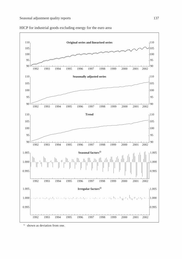
Seasonal adjustment quality reports 137
1992 1993 1994 1995 1996 1997 1998 1999 2000 2001 200290
95
100
105
110
90
95
100
105
110Original series and linearised series
1992 1993 1994 1995 1996 1997 1998 1999 2000 2001 200290
95
100
105
110
90
95
100
105
110Seasonally adjusted series
1992 1993 1994 1995 1996 1997 1998 1999 2000 2001 200290
95
100
105
110
90
95
100
105
110Trend
1992 1993 1994 1995 1996 1997 1998 1999 2000 2001 2002
0.995
1.000
1.005
0.995
1.000
1.005Seasonal factors1)
1992 1993 1994 1995 1996 1997 1998 1999 2000 2001 2002
0.995
1.000
1.005
0.995
1.000
1.005Irregular factors1)
HICP for industrial goods excluding energy for the euro area
1) shown as deviation from one.
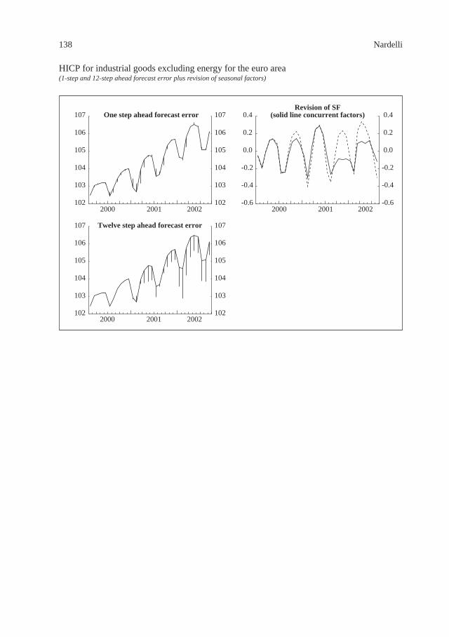
138 Nardelli
HICP for industrial goods excluding energy for the euro area(1-step and 12-step ahead forecast error plus revision of seasonal factors)
2000 2001 2002102
103
104
105
106
107
102
103
104
105
106
107One step ahead forecast error
2000 2001 2002102
103
104
105
106
107
102
103
104
105
106
107Twelve step ahead forecast error
2000 2001 2002-0.6
-0.4
-0.2
0.0
0.2
0.4
-0.6
-0.4
-0.2
0.0
0.2
0.4Revision of SF
(solid line concurrent factors)

Seasonal adjustment quality reports 139
SPECIFICATION FILE FOR icp.m.i2.n.igxe00.4.inx
1 2 # 3 # Specification set: ICP_I2_IGXE00 4 # Description: Industrial goods (excl. energy) index for the euro area (MU-12) 5 # 6 SERIES 7 { 8 FILE = "icp.m.i2.n.igxe00.4.inx.dat" 9 FORMAT = DATEVALUE 10 NAME = "ICP.M.I2.N.IGXE00.4.INX" 11 PERIOD = 12 12 } 13 # 14 TRANSFORM 15 { 16 FUNCTION = LOG 17 } 18 # 19 X11 20 { 21 APPENDFCST = YES 22 CALENDARSIGMA = ALL 23 MODE = MULT 24 SAVE = (TREND TRENDD7 UNMODSI REPLACSI SEASONAL SEASADJ IRREGULAR 25 ADJUSTFAC IRRWT ADJORIGINAL) 26 SAVELOG = (M1 M2 M3 M4 M5 M6 M7 M8 M9 M10 M11 Q Q2 MOVINGSEASRATIO 27 ICRATIO FSTABLEB1 FSTABLED8 MOVINGSEASF IDSEASONAL) 28 SEASONALMA = S3X1 29 SIGMALIM = (2.0,3.5) 30 } 31 # 32 REGRESSION 33 { 34 AICTEST = (USER) 35 SAVE = (LEVELSHIFT TEMPORARYCHANGE AOUTLIER) 36 VARIABLES = (LS2001.Mar) 37 } 38 # 39 ARIMA 40 { 41 MODEL = (0,1,1)(0,1,1)12 42 } 43 # 44 ESTIMATE 45 { 46 SAVE = (RESIDUALS ESTIMATES ROOTS) 47 SAVELOG = (AIC AICC BIC AVERAGEFCSTERR) 48 } 49 # 50 OUTLIER 51 { 52 CRITICAL = 4.5 53 TYPES = ALL 54 } 55 # 56 CHECK 57 { 58 SAVELOG = (NORMALITYTEST LJUNGBOXQ) 59 } 60 # 61 HISTORY 62 { 63 ESTIMATES = (FCST SEASONAL) 64 SAVE = (FCSTHISTORY SFREVISIONS) 65 SAVELOG = (AVEABSREVCHNG AVEABSREVINDSA AVEABSREVTREND 66 AVEABSREVTRENDCHNG AVEABSREVSF AVEABSREVSFPROJ) 67 START = 2000.Jan 68 } 69 #

140 Nardelli
One and twelve step ahead Revision of seasonal factorsforecast error (concurrent/forecast)
1-step 12-step Concurrent Projected
Feb. 2000 -0.062 -- Jan. 2000 -0.049 -0.056Mar. 0.101 -- Feb. -0.188 -0.200Apr. -0.040 -- Mar. -0.018 -0.007May 0.001 -- Apr. 0.121 0.129June 0.086 -- May 0.135 0.141July -0.231 -- June 0.052 0.076Aug. 0.200 -- July -0.243 -0.271Sep. 0.188 -- Aug. -0.244 -0.231Oct. 0.099 -- Sep. -0.046 0.010Nov. 0.095 -- Oct. 0.099 0.170Dec. 0.064 -- Nov. 0.144 0.222Jan. 2001 -0.492 0.060 Dec. 0.076 0.155Feb. -0.456 -0.385 Jan. 2001 -0.061 -0.117Mar. 0.834 0.238 Feb. -0.310 -0.402Apr. 0.439 0.722 Mar. 0.048 -0.068May 0.079 0.909 Apr. 0.246 0.244June -0.056 0.778 May 0.282 0.293July -0.415 0.602 June 0.187 0.174Aug. -0.152 0.132 July -0.073 -0.240Sep. 0.466 0.353 Aug. -0.269 -0.352Oct. 0.240 0.632 Sep. -0.159 -0.062Nov. 0.028 0.638 Oct. -0.091 0.177Dec. 0.020 0.602 Nov. -0.095 0.232Jan. 2002 -0.040 1.072 Dec. -0.092 0.171Feb. 0.135 1.708 Jan. 2002 -0.117 -0.114Mar. 0.565 1.582 Feb. -0.238 -0.260Apr. -0.015 1.113 Mar. 0.085 0.226May -0.118 0.920 Apr. 0.112 0.333June -0.034 0.912 May 0.085 0.275July -0.188 1.178 June 0.120 0.152Aug. -0.051 1.220 July 0.009 -0.025Sep. 0.085 0.750 Aug. -0.126 -0.304
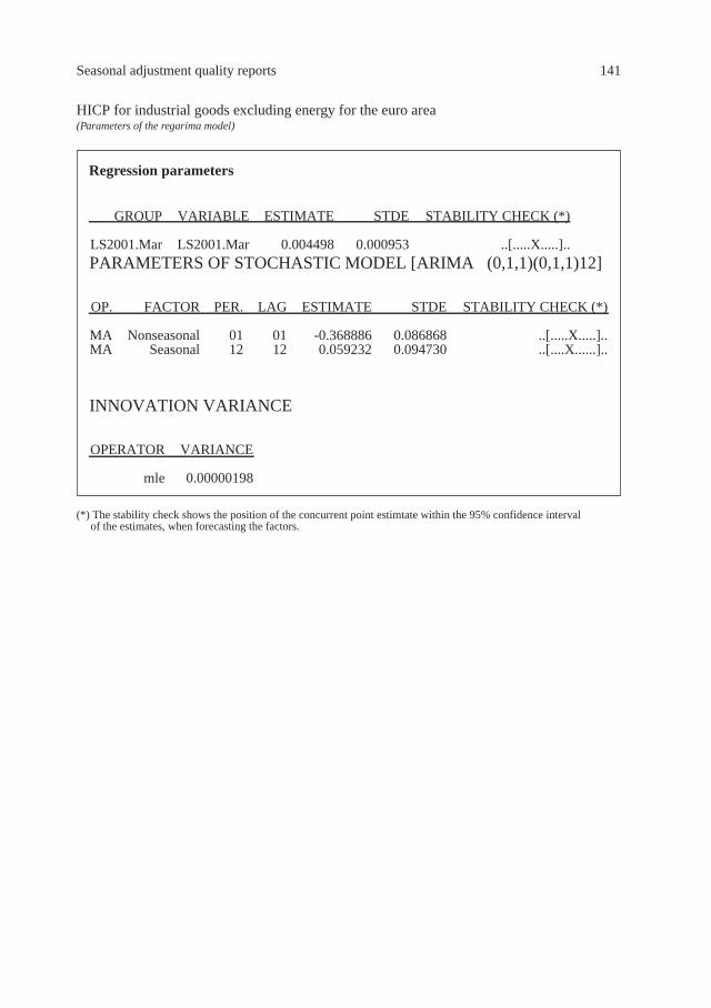
Seasonal adjustment quality reports 141
GROUP VARIABLE ESTIMATE STDE STABILITY CHECK (*)
LS2001.Mar LS2001.Mar 0.004498 0.000953 ..[.....X.....]..PARAMETERS OF STOCHASTIC MODEL [ARIMA (0,1,1)(0,1,1)12]
OP. FACTOR PER. LAG ESTIMATE STDE STABILITY CHECK (*)
MA Nonseasonal 01 01 -0.368886 0.086868 ..[.....X.....]..MA Seasonal 12 12 0.059232 0.094730 ..[....X......]..
INNOVATION VARIANCE
OPERATOR VARIANCE
mle 0.00000198
(*) The stability check shows the position of the concurrent point estimtate within the 95% confidence interval of the estimates, when forecasting the factors.
HICP for industrial goods excluding energy for the euro area(Parameters of the regarima model)
Regression parameters

142 Nardelli
CRITERIA PARAMETER VALUE
Average Absolute Percentage Error within-sample forecasts AAPE(Last year) 0.52
AAPE(Last-1 year) 0.26 AAPE(Last-2 year) 0.16 AAPE(Last 3 years) 0.31
AIC -116.0806 AICC -115.7203
BIC -105.0663 Summary of Significant Ljung-Box Q
Lag Q DF P --- ------- --- -----
6 16.445 4 0.002 7 18.044 5 0.003 8 29.511 6 0.000 9 29.517 7 0.000
10 30.530 8 0.000 11 31.675 9 0.000
12 31.686 10 0.000 13 31.744 11 0.001 14 35.903 12 0.000 15 37.201 13 0.000 16 37.314 14 0.001 17 38.322 15 0.001 18 43.330 16 0.000 19 48.277 17 0.000 20 48.277 18 0.000 21 49.579 19 0.000 22 49.769 20 0.000 23 49.819 21 0.000 24 50.839 22 0.000
Geary's a statistic 0.7424 (significant) Kurtosis 4.2768
Moving seasonality ratio 1.531 I/C Ratio 0.397
Stable Seasonal F, B1 table 26.133 Stable Seasonal F, D8 table 32.239
Moving Seasonal F, D8 table 12.695 Identifiable seasonality yes
M01 0.055 M02 0.015 M03 0.000 M04 0.462 M05 0.000 M06 0.988 M07 0.836 M08 1.417 M09 1.274 M10 1.430 M11 1.320
Q 0.548 Q2 0.622
AveAbsRev of Seasonal 0.132 AveAbsRev of Projected Seasonal 0.184
HICP for industrial goods excluding energy for the euro area(Quality criteria of X-11)
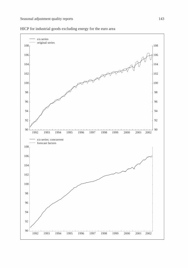
Seasonal adjustment quality reports 143
1992 1993 1994 1995 1996 1997 1998 1999 2000 2001 200290
92
94
96
98
100
102
104
106
108
90
92
94
96
98
100
102
104
106
108
s/a seriesoriginal series
1992 1993 1994 1995 1996 1997 1998 1999 2000 2001 200290
92
94
96
98
100
102
104
106
108
s/a series: concurrentforecast factors
HICP for industrial goods excluding energy for the euro area

144 Nardelli
B1 HICP for industrial goods excluding energy for the euro area
Jan. Feb. Mar. Apr. May June July Aug. Sep. Oct. Nov. Dec. AVGE
1992 90.957 91.349 91.842 92.027 92.209 92.206 92.183 92.417 92.803 93.096 93.486 93.536 92.3431993 93.713 94.263 94.788 94.942 95.145 95.263 95.136 95.319 95.639 95.987 96.151 96.143 95.2071994 96.148 96.381 96.794 96.870 97.001 96.957 96.747 96.883 97.267 97.541 97.678 97.733 97.0001995 97.624 97.987 98.422 98.600 98.732 98.837 98.538 98.825 99.353 99.634 99.850 99.829 98.8531996 99.512 99.843 100.427 100.494 100.591 100.588 100.197 100.284 100.686 100.956 100.891 100.933 100.4501997 100.470 100.751 101.190 101.231 101.267 101.123 100.634 100.815 101.304 101.499 101.653 101.648 101.1321998 101.123 101.500 101.996 102.236 102.328 102.283 101.757 102.001 102.502 102.639 102.709 102.688 102.1471999 102.098 102.397 102.874 102.951 103.028 102.956 102.393 102.645 102.990 103.182 103.279 103.239 102.8362000 102.660 102.914 103.490 103.572 103.646 103.663 102.889 103.308 103.899 104.206 104.408 104.451 103.5922001 103.381 103.135 103.964 104.490 104.754 104.716 103.556 103.681 104.655 105.325 105.617 105.677 104.4132002 104.638 104.588 105.778 106.371 106.498 106.387 105.050 105.082 106.107 106.793 107.083 107.142 105.960
D8 HICP for industrial goods excluding energy for the euro area
Jan. Feb. Mar. Apr. May June July Aug. Sep. Oct. Nov. Dec. AVGE
1992 99.788 99.999 100.310 100.284 100.255 100.017 99.749 99.745 99.900 99.955 100.107 99.872 99.9981993 99.762 100.054 100.337 100.241 100.207 100.091 99.728 99.712 99.863 100.059 100.076 99.932 100.0051994 99.823 99.955 100.267 100.218 100.214 100.033 99.692 99.713 99.990 100.141 100.127 100.010 100.0151995 99.723 99.925 100.204 100.221 100.181 100.102 99.610 99.705 100.038 100.137 100.202 100.058 100.0091996 99.626 99.837 100.290 100.218 100.187 100.085 99.621 99.655 100.021 100.251 100.134 100.113 100.0031997 99.594 99.823 100.224 100.249 100.266 100.094 99.564 99.677 100.072 100.166 100.223 100.132 100.0071998 99.530 99.804 100.179 100.287 100.260 100.116 99.515 99.681 100.107 100.188 100.209 100.141 100.0011999 99.521 99.772 100.202 100.238 100.253 100.118 99.523 99.751 100.095 100.283 100.328 100.180 100.0222000 99.487 99.632 100.142 100.211 100.253 100.181 99.309 99.599 100.081 100.308 100.458 100.491 100.0132001 99.493 99.286 LS100.052 LS 100.437 LS+1 100.533 100.369 99.172 99.204 100.002 100.468 100.572 100.481 100.0062002 99.359 99.171 100.155 100.589 100.614 100.442 99.112 99.055 99.908 -- -- -- --
Seasonal factors of concurrent run2001 99.438 99.359 100.158 100.474 100.519 100.326 99.189 99.283 100.000 100.400 100.526 100.400 100.0062002 99.424 99.222 100.172 100.551 100.593 100.413 99.123 99.101 99.943 100.436 100.560 100.485 100.002
Seasonal factors officially in use2001 99.420 99.422 100.115 100.381 100.445 100.303 99.217 99.475 100.028 100.408 100.516 100.379 100.0092002 99.399 99.262 100.090 100.438 100.523 100.371 99.179 99.368 99.991 100.453 100.556 100.464 100.008
D9 HICP for industrial goods excluding energy for the euro area
Jan. Feb. Mar. Apr. May June July Aug. Sep. Oct. Nov. Dec. AVGE
1992 -- -- -- -- -- -- -- -- -- -- -- -- --1993 -- -- -- -- -- -- -- -- 99.972 -- -- -- --1994 99.741 -- -- -- -- -- -- -- -- -- -- -- --1995 -- -- -- -- -- -- -- -- -- -- -- -- --1996 -- -- -- -- -- -- -- -- -- -- -- -- --1997 -- -- -- -- -- -- -- -- -- -- -- -- --1998 -- -- -- -- -- -- -- -- -- -- -- -- --1999 -- -- -- -- -- -- 99.399 -- -- -- -- -- --2000 -- -- -- 100.372 100.400 -- -- -- -- -- -- 100.254 --2001 -- -- 100.153 -- -- -- -- -- -- -- -- -- --2002 -- -- -- -- -- -- -- -- -- -- -- -- --

Seasonal adjustment quality reports 145
D10 HICP for industrial goods excluding energy for the euro area
Jan. Feb. Mar. Apr. May June July Aug. Sep. Oct. Nov. Dec. AVGE
1992 99.755 100.018 100.318 100.265 100.234 100.043 99.738 99.731 99.928 99.997 100.098 99.899 100.0021993 99.751 100.008 100.309 100.248 100.224 100.043 99.718 99.721 99.954 100.054 100.107 99.942 100.0071994 99.728 99.985 100.275 100.228 100.199 100.069 99.669 99.707 100.001 100.114 100.137 100.003 100.0101995 99.691 99.912 100.260 100.222 100.194 100.070 99.637 99.690 100.018 100.178 100.155 100.060 100.0071996 99.644 99.864 100.241 100.230 100.210 100.089 99.594 99.678 100.045 100.186 100.185 100.098 100.0051997 99.597 99.822 100.231 100.249 100.235 100.094 99.563 99.670 100.068 100.204 100.190 100.128 100.0041998 99.561 99.804 100.203 100.258 100.257 100.103 99.487 99.701 100.094 100.214 100.251 100.146 100.0071999 99.516 99.738 100.177 100.300 100.300 100.129 99.398 99.676 100.101 100.265 100.330 100.183 100.0092000 99.478 99.568 100.178 100.359 100.396 100.214 99.281 99.515 100.066 100.355 100.445 100.288 100.0122001 99.438 99.359 100.158 100.474 100.519 100.326 99.189 99.283 100.000 100.400 100.526 100.400 100.0062002 99.424 99.222 100.172 100.551 100.593 100.413 99.123 99.101 99.943 100.436 100.560 100.485 100.002
Jan. Feb. Mar. Apr. May June July Aug. Sep. Oct. Nov. Dec. AVGE
1992 90.757 90.947 91.149 91.356 91.567 91.785 92.003 92.228 92.460 92.700 92.956 93.237 91.9291993 93.527 93.803 94.060 94.302 94.536 94.761 94.969 95.153 95.315 95.476 95.636 95.780 94.7771994 95.898 96.003 96.107 96.220 96.350 96.484 96.608 96.728 96.847 96.978 97.130 97.296 96.5541995 97.459 97.613 97.768 97.930 98.106 98.297 98.488 98.679 98.870 99.048 99.197 99.322 98.3981996 99.441 99.563 99.691 99.825 99.946 100.042 100.119 100.177 100.218 100.259 100.309 100.366 99.9961997 100.420 100.469 100.508 100.533 100.557 100.588 100.630 100.691 100.775 100.871 100.965 101.052 100.6711998 101.140 101.239 101.356 101.489 101.613 101.719 101.806 101.871 101.922 101.965 102.014 102.076 101.6841999 102.137 102.181 102.203 102.228 102.285 102.366 102.438 102.468 102.461 102.456 102.504 102.611 102.3612000 102.732 102.811 102.835 102.838 102.882 102.999 103.151 103.280 103.370 103.438 103.486 103.494 103.1102001 103.455 103.409 103.893 104.009 104.170 104.306 104.406 104.513 104.671 104.869 105.054 105.193 104.3292002 105.308 105.439 105.594 105.748 105.867 105.935 105.989 106.063 106.178 -- -- -- --
D12 HICP for industrial goods excluding energy for the euro area
D11 HICP for industrial goods excluding energy for the euro area
Jan. Feb. Mar. Apr. May June July Aug. Sep. Oct. Nov. Dec. AVGE
1992 90.771 90.923 91.140 91.373 91.581 91.753 92.010 92.250 92.453 92.681 92.976 93.211 91.9271993 93.525 93.832 94.072 94.281 94.507 94.794 94.976 95.157 95.254 95.505 95.617 95.767 94.7741994 95.977 95.962 96.096 96.217 96.375 96.456 96.633 96.731 96.830 96.993 97.106 97.291 96.5551995 97.487 97.633 97.726 97.940 98.099 98.325 98.454 98.687 98.889 99.010 99.248 99.322 98.4021996 99.420 99.530 99.735 99.814 99.930 100.048 100.154 100.156 100.189 100.316 100.253 100.381 99.9941997 100.424 100.478 100.504 100.526 100.576 100.574 100.621 100.695 100.781 100.838 101.006 101.063 100.6741998 101.114 101.243 101.332 101.515 101.608 101.720 101.823 101.847 101.947 101.960 101.992 102.078 101.6821999 102.134 102.205 102.231 102.183 102.259 102.362 102.551 102.517 102.424 102.448 102.476 102.588 102.3652000 102.736 102.897 102.842 102.738 102.774 102.978 103.169 103.346 103.365 103.371 103.479 103.684 103.1152001 103.499 103.334 103.800 103.996 104.214 104.376 104.403 104.430 104.656 104.905 105.064 105.255 104.3282002 105.245 105.408 105.597 105.788 105.871 105.950 105.979 106.036 106.167 -- -- -- --
Seasonally adjusted series when using the official forecast seasonal/trading day factors2001 103.518 103.269 103.844 104.093 104.290 104.400 104.373 104.229 104.627 104.897 105.074 105.278 104.3242002 105.271 105.366 105.684 105.907 105.944 105.994 105.920 105.751 106.116 -- -- -- --
Month to month percentage variation concurrent run2001 -0.2 -0.2 0.5 0.2 0.2 0.2 0.0 0.0 0.2 0.2 0.2 0.2 0.12002 -0.0 0.2 0.2 0.2 0.1 0.1 0.0 0.1 0.1 -- -- -- --
Month to month percentage variation when using the official forecast seasonal/trading day factors2001 -0.2 -0.2 0.6 0.2 0.2 0.1 -0.0 -0.1 0.4 0.3 0.2 0.2 0.12002 -0.0 0.1 0.3 0.2 0.0 0.0 -0.1 -0.2 0.3 -- -- -- --

146 Nardelli
D13 HICP for industrial goods excluding energy for the euro area
Jan. Feb. Mar. Apr. May June July Aug. Sep. Oct. Nov. Dec. AVGE
1992 100.015 99.973 99.990 100.018 100.015 99.966 100.008 100.023 99.992 99.979 100.021 99.971 99.9981993 99.998 100.031 100.013 99.978 99.969 100.035 100.008 100.004 99.935 100.030 99.980 99.987 99.9971994 100.082 99.958 99.988 99.996 100.025 99.971 100.026 100.004 99.982 100.015 99.975 99.995 100.0011995 100.029 100.020 99.957 100.011 99.992 100.028 99.965 100.008 100.019 99.962 100.051 100.000 100.0031996 99.979 99.967 100.044 99.990 99.984 100.006 100.036 99.979 99.971 100.057 99.943 100.015 99.9981997 100.005 100.009 99.996 99.994 100.019 99.987 99.992 100.004 100.006 99.968 100.040 100.010 100.0021998 99.974 100.004 99.976 100.026 99.995 100.000 100.017 99.977 100.025 99.995 99.978 100.002 99.9971999 99.998 100.024 100.027 99.956 99.974 99.996 100.111 100.047 99.964 99.992 99.974 99.977 100.0032000 100.004 100.083 100.007 99.904 99.895 99.980 100.017 100.064 99.996 99.935 99.993 100.184 100.0052001 100.042 99.928 99.910 99.988 100.042 100.068 99.997 99.921 99.985 100.035 100.010 100.059 99.9992002 99.940 99.971 100.003 100.037 100.004 100.014 99.990 99.974 99.989 -- -- -- --
D16 HICP for industrial goods excluding energy for the euro area
Jan. Feb. Mar. Apr. May June July Aug. Sep. Oct. Nov. Dec. AVGE
1992 99.755 100.018 100.318 100.265 100.234 100.043 99.738 99.731 99.928 99.997 100.098 99.899 100.0021993 99.751 100.008 100.309 100.248 100.224 100.043 99.718 99.721 99.954 100.054 100.107 99.942 100.0071994 99.728 99.985 100.275 100.228 100.199 100.069 99.669 99.707 100.001 100.114 100.137 100.003 100.0101995 99.691 99.912 100.260 100.222 100.194 100.070 99.637 99.690 100.018 100.178 100.155 100.060 100.0071996 99.644 99.864 100.241 100.230 100.210 100.089 99.594 99.678 100.045 100.186 100.185 100.098 100.0051997 99.597 99.822 100.231 100.249 100.235 100.094 99.563 99.670 100.068 100.204 100.190 100.128 100.0041998 99.561 99.804 100.203 100.258 100.257 100.103 99.487 99.701 100.094 100.214 100.251 100.146 100.0071999 99.516 99.738 100.177 100.300 100.300 100.129 99.398 99.676 100.101 100.265 100.330 100.183 100.0092000 99.478 99.568 100.178 100.359 100.396 100.214 99.281 99.515 100.066 100.355 100.445 100.288 100.0122001 99.438 99.359 100.158 100.474 100.519 100.326 99.189 99.283 100.000 100.400 100.526 100.400 100.0062002 99.424 99.222 100.172 100.551 100.593 100.413 99.123 99.101 99.943 100.436 100.560 100.485 100.002
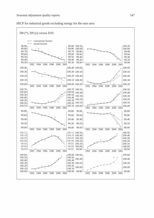
Seasonal adjustment quality reports 147
HICP for industrial goods excluding energy for the euro area
concurrent factorssaved factors
1992 1994 1996 1998 2000 2002
1992 1994 1996 1998 2000 2002
1992 1994 1996 1998 2000 2002
1992 1994 1996 1998 2000 2002
1992 1994 1996 1998 2000 2002
1992 1994 1996 1998 2000 2002
99.3099.4099.5099.6099.7099.8099.90
99.0099.2099.4099.6099.80
100.00100.20
100.00
100.10
100.20
100.30
100.40
100.20
100.30
100.40
100.50
100.60
100.10100.20100.30100.40100.50100.60100.70
100.00100.10100.20100.30100.40100.50
99.00
99.20
99.40
99.60
99.80
99.00
99.20
99.40
99.60
99.80
99.8599.9099.95
100.00100.05100.10100.15
99.90100.00100.10100.20100.30100.40100.50
100.00100.10100.20100.30100.40100.50100.60
99.3099.4099.5099.6099.7099.8099.90
100.00
100.10
100.20
100.30
100.40
100.10100.20100.30100.40100.50100.60100.70
99.00
99.20
99.40
99.60
99.80
99.8599.9099.95
100.00100.05100.10100.15
100.00100.10100.20100.30100.40100.50100.60
99.80
100.00
100.20
100.40
100.60
99.0099.2099.4099.6099.80
100.00100.20
100.20
100.30
100.40
100.50
100.60
100.00100.10100.20100.30100.40100.50
99.00
99.20
99.40
99.60
99.80
99.90100.00100.10100.20100.30100.40100.50
99.80
100.00
100.20
100.40
100.60
1992 1994 1996 1998 2000 2002
1992 1994 1996 1998 2000 2002
1992 1994 1996 1998 2000 2002
1992 1994 1996 1998 2000 2002
1992 1994 1996 1998 2000 2002
1992 1994 1996 1998 2000 2002
D8 (*), D9 (o) versus D10

148 Nardelli

9
The performance of X-12 in the seasonal adjustment of shorttime series
Antonio Matas Mir and Vitaliana Rondonotti
1. Introduction
The European Central Bank (ECB) currently produces seasonally adjusted data for euro areamonetary aggregates and counterparts (8 series in total). These series cover a period of morethan 20 years (with the exception for loans for which data is available as from January 1991).The approach used relies on multiplicative decomposition through X-12-ARIMA. For detailssee “Seasonal adjustment of monetary aggregates and HICP for the euro area”, ECB (2000).
Seasonally and calendar adjusted data for further items of the consolidated balance sheet ofthe MFI sector are currently under development. At present, these series include only 5 yearsof data. Thus, there is an important need for studying from several perspectives the potentialquality of such adjustments as compared to those already routinely produced by the ECB forthe main monetary aggregates, which are based on historical series beginning in 1980.
This paper aims to make a contribution to such an assessment by means of the applicationof Monte Carlo simulation techniques1. For this purpose we will evaluate the performance ofX-12-ARIMA using simulated economic time series of 5 years of data and compare theresults to its performance on simulated time series with 15 years of additional historical data.The exercise considers different stochastic properties for the seasonal and trend components,the effect of different forecast/backcast extension options and the effect of outliers on thequality of the adjustment.
For the purpose of this evaluation, we will therefore restrict ourselves to the following:• X-12-ARIMA (version 0.2.2), which is the method currently used at the ECB. The X-12-
ARIMA seasonal adjustment program is based on the X-11 program (Shiskin, Young andMusgrave 1967) and Statistics Canada’s X-11-ARIMA and X-11-ARIMA/88 (Dagum,1988). For details of X-12-ARIMA see Findley, Monsell, Bell, Otto and Chen (1998) andU.S. Census Bureau (2002).
• Simulated time series with stochastic properties similar to the ones of a real monetaryseries currently seasonally adjusted by the ECB. In order to have a more complete set of theresults, different values for the parameters of the models and the effect of different type ofoutliers will also be considered.
• Simulated time series of 5 years of data where no historical data is available (hereafterreferred to as “short time series”), where 15 years of historical data are available (hereafterreferred to as “long time series”), and where 7 years of data at each end of the time seriesare available.
1 No similar study appears to have been conducted to date. Hood, Ashley and Findley (2000) examinethe issue of the seasonal adjustment of short time series in a comparison between TRAMO/SEATS andX-12 ARIMA, although their approach is not based on parametric Monte Carlo simulation.

150 Matas Mir and Rondonotti
• Accuracy measures of the adjustment of the simulated series based primarily on how closethe estimates of the monthly growth rates are to the “final” estimates, where by “final”estimates we indicate the seasonal adjustment for the simulated time series of 5 years ofdata obtained by making use of an additional 7 years of data at each end of the time series.
2. Methodology
Consider xft as being the result of seasonally adjusting the series xt for t = 1,...,60 (5 years of
data) making use of data spanning from t = -84 to t = 144 (i.e. making use of 7 years ofadditional data at each end). Thus, xf
t represents what is usually referred to as “finaladjustment”, in the sense that consideration of additional data on xt for t > 144 or t < -84should not fundamentally change the result of the adjustment.2 Now consider xs
t as being theresult of seasonally adjusting the series xt for t = 1,...,60 making use only of data from t = 1 tot = 60. Thus, this represents the situation in which the practitioner adjusts a sample of 5 yearsof data for which no observations are available before or after the series being adjusted.Finally, define xl
t as the result of adjusting the series xt for t = 1,...,60 making use of anhistorical time series spanning 15 years in the past from the initial observation to be adjusted,t = 1.
We aim at assessing the loss in adjustment quality in xst as compared to xl
t deriving from thefact that, being xs
t a series of only 5 years, there may not be enough information in the sampleto obtain sufficiently accurate adjustments. In opposition, as xl
t utilises information spanninga total of 20 years of data, it is considered to be a good benchmark against which such qualitymay be assessed.
In order to do this, we will study for both cases, xlt and xs
t, the behaviour of the deviationsfrom the “final” adjustment xf
t by means of Monte Carlo simulation techniques. Specifically,we draw replications from the following airline model
∆∆12xt = (1 – θL)(1 – ΘL12)at [1]where at ~ NID(0, � 2
a)whose parameters have been chosen to match those estimated from the chain index of theeuro area monetary aggregate other short term deposits.3 We will refer throughout to thisspecific parameterisation as our “baseline model”, as later on we will introduce some changesin the parameters for sensitivity analysis purposes. Then, for each replication, we obtain theadjustments xf
t, xlt, and xs
t by making use of the relevant data spans as mentioned before.4 Foreach replication we can compute the deviations of xl
t and xst from the “final adjustment”.
However, we have opted to focus instead on the behaviour of the monthly growth rate of the
2 See, for instance, the discussion of the linear approximation to X-11 in Wallis (1974). Note that, strictlyspeaking, this applies to an adjustment making use exclusively of the X-11 filters with default options. Non-default seasonal filters, X-12 preadjustment and X-12 forecast options change the picture. However, sinceno preadjustment or forecast extension will be needed to determine x f
t in our simulations the issue can beignored, and as for the possible change to non-default seasonal filters it should be expected that filter weightsat lags or leads beyond 7 years should be very small.
3 Specifically, the estimates for this series for the period January 80 – August 2002 are θ = -0.11, Θ = 0.54,� 2
a = 1.2 × 10⁻⁵. Starting values were chosen so that the seasonal pattern and long-run trend matched on averagethose of the empirical series.
4 X-12 ARIMA has been run in each case with standard options with the following exceptions: for thecomputation of x f
t all preadjustment and forecast extension options are disabled (as they should not beinvoked); for the computation of xs
t MAXBACK is set to 12 in the FORECAST spec. In the case of xst and, xl
t,ARIMA model selection is left to X-12’s automatic selection procedure.

The performance of X-12 in the seasonal adjustment of short time series 151
series, a more relevant magnitude from the perspective of most economic analyses. Thus, wedefine the absolute deviations δ l
t =x.lt – x
.ft and δ s
t =x.st – x
. ft , where x
.it stands for the monthly
growth rate of the relevant seasonally adjusted series for i = f,l. By studying the propertiesof δ l
t and δ st and we may obtain important insights into the potential problems associated with
the seasonal adjustment of short time series.5
3. Results for the baseline model
Figure 1 (a) plots the median across 1000 Monte Carlo replications of δ lt and δ s
t fort = 1,...,60. In order to facilitate the reader in assessing the practical importance of themagnitudes of δ l
t and δ st , these are expressed in terms of the impact that such deviations
would imply for the month-to-month growth rate expressed at annual rates.6 As expected,the graph shows a larger discrepancy with respect to the final adjustment for the shorttime series across the whole time range.
Specifically, as it can be seen in Figure 1 (a), in the first and the second year of the sample,the adjustment using the short time series performs very poorly in comparison with the resultsfor the long time series. Indeed, the discrepancy δ s
t may be as large as 120 basis points (inmedian terms), compared to only 20 basis points for δ l
t. This is mainly due to the fact that inthe case of the short time series, data have to be backcasted, while these data are available inthe long time series. Furthermore, when using the short time series, complete application ofthe X-11 symmetric filters is not possible during the first years of data.
In contrast, in the last two years of data the magnitude of δ lt increases considerably and
becomes closer to the magnitude of δ st . The rationale behind this is that, as one approaches the
end of the time series, data have to be forecasted in both cases, long sample and short sample,and in neither case is the complete use of symmetric filters feasible.
Similar conclusions may be derived from a synthetic measure of the accuracy of theadjustment. We derive such measure as the mean absolute deviation (MAD) from the finaladjustment. This is computed for the whole sample and then separately for its first and secondhalves. The relevant expected values as estimated from 1000 Monte Carlo replications arepresented in Table 1. The mean absolute deviation (MAD) with respect to the final adjustmentturns out to be larger by a factor (hereafter referred to as the “MAD ratio”) of 1.55 for theseries using 5 years of data (T=60) compared to the long historical time series (T=240). Thisresult is however compounded by a very large MAD ratio of 2.69 for the first half of thesample, and a relatively moderate value of 1.09 for the second half.
5 From a more general perspective, our results will represent in fact a lower bound on the loss associatedwith adjustment using a small sample. Indeed, if one sees seasonal adjustment as a signal extraction problem,issues such as the additional uncertainty in the inference about the optimal seasonal adjustment filter wouldhave to be taken into account. By restricting ourselves to X-12 ARIMA, these issues are side-stepped, as theX-12 filters have, to a great extent, fixed weights. For an approach to seasonal adjustment based on optimalsignal extraction theory, see Gomez and Maravall (1996).
6 Such annualisation is not totally invariant to the actual growth rate of the series, although differences areminor if one considers the range of plausible growth rates for a major monetary aggregate in the euro area. Wehave considered an annual growth rate of 5% to implement it.

152 Matas Mir and Rondonotti
Figure 1: Median absolute discrepancy with respect to final seasonal adjustmentfor short time series (T=60) and long time series (T=240)(Discrepancy expressed in terms of impact on annualised monthly growth rate)
0
0.2
0.4
0.6
0.8
1
1.2
1.4
1.6
1.8
0 5 10 15 20 25 30 35 40 45 50 55
(a) Baseline model
T=60
T=240
0
0.2
0.4
0.6
0.8
1
1.2
1.4
1.6
1.8
0
0.2
0.4
0.6
0.8
1
1.2
1.4
1.6
1.8
0 5 10 15 20 25 30 35 40 45 50 55
(b) Highly stochastic seasonal
T=60
T=240
0
0.2
0.4
0.6
0.8
1
1.2
1.4
1.6
1.8
0
0.2
0.4
0.6
0.8
1
1.2
1.4
1.6
1.8
0
0.2
0.4
0.6
0.8
1
1.2
1.4
1.6
1.8
0 5 10 15 20 25 30 35 40 45 50 55
(c) Highly deterministic seasonal
T=60
T=240

The performance of X-12 in the seasonal adjustment of short time series 153
4. Changing the nature of the seasonal cycle and the trend
In order to assess the impact of a different seasonal behaviour of the time series, our analysisneeds now to consider setting different values of Θ in [1]. For instance, by setting Θ = 0, alarger degree of variability in the seasonal pattern is introduced7. As it is shown in Figure 1(b),this results in a much larger magnitude for δ s
t across the whole time range. In contrast, δ lt only
increases to a similar degree in the last two years of data. Thus, the unavailability of longhistorical data coupled with the fact that backcasting becomes more difficult due to the highvariability of the seasonal implies that the loss in quality dramatically increases for the shorttime series in the first half of the sample.
Next we consider a more stable seasonal pattern by setting Θ = 0.95. The results of theMonte Carlo analysis for this parameterisation of the model are shown in Figure 1 (c). Themost salient feature, apart from the reduction in the magnitude of both discrepancies δ s
t andδ l
t, is that the superior behaviour of the adjustment using the long series is now alsonon-negligible even for the last two years of the sample. The reason behind this is that, withΘ = 0.95, the seasonal pattern becomes more predictable, and hence more amenable to beingeasily extrapolated beyond the available data by means of forecasts. In such case, theadvantages of having a better forecasting model (which should in principle be the case whenusing a long time series for estimation) increase, hence the larger difference between δ s
t and δ lt
towards the end of the sample as compared with previous cases. This shows up clearly in theMAD ratio (see Table 1), which for the second half of the sample goes up to 1.27 in the caseof a highly deterministic seasonal from 1.09 observed when the seasonal is mediumstochastic and 1.03 when it is highly stochastic.
The analysis has also considered the impact of a different stochastic nature of the trend.From the figures in Table 1 it is clear that, as the trend becomes more deterministic, the loss inthe quality of the adjustment derived by using a short time series increases significantly in thefirst part of the sample. This is mainly due to the fact that the magnitude of δ l
t reducessignificantly with a more stable trend, whereas this is not so much the case for δ s
t (possibly thebackcasts used in the short time series do not benefit in excess from a more stable trend as
7 In every instance in this study where the value of a parameter in [1] has been changed from our baselinemodel, the variance of the innovation �2
a in the DGP has been suitably rescaled so that the unconditionalvariance of the stationary transformation of the series var(∆∆12xt) = σ 2
a (1+θ 2+Θ2+θ 2Θ2) remains invariant tothe different specific parameterisations.
Table 1: Sensitivity to different time-series properties
All observations t<=30 t>30(a) (b) Ratio (a) (b) Ratio (a) (b) Ratio
T=240 T=60 (b/a) T=240 T=60 (b/a) T=240 T=60 (b/a)
Highly stochastic seasonal 1.019 1.638 1.61 0.470 1.638 3.49 1.587 1.638 1.03Baseline (Medium stochastic seasonal) 0.721 1.119 1.55 0.410 1.103 2.69 1.043 1.136 1.09Highly deterministic seasonal 0.414 0.775 1.87 0.223 0.772 3.46 0.611 0.778 1.27
Baseline (Highly stochastic trend) 0.721 1.119 1.55 0.410 1.103 2.69 1.043 1.136 1.09Medium stochastic trend 0.572 0.977 1.71 0.270 0.982 3.63 0.885 0.972 1.10Highly deterministic trend 0.599 0.981 1.64 0.250 0.965 3.86 0.959 0.997 1.04
All figures represent the mean absolute deviation with respect to final seasonal adjustment and are expressedin terms of impact on percent annualised monthly growth rate.

154 Matas Mir and Rondonotti
they do from a more stable seasonal). This implies an increase in the MAD ratio, for the firsthalf of the sample, from 2.69 in the case of a highly stochastic trend to 3.86 when the trendbecomes highly deterministic.
5. Changing the X-12 forecasting/backcasting options
Our analysis takes now into consideration different forecasting/backcasting options, in orderto check whether our results are dependent in excess on the particular forecasting optionschosen for our baseline model (default 12-month forecasts, 12-month backcasts for the shorttime series). We also aim at answering the question of whether it would be preferable todisable the backasting/forecasting extension in the case of the short time series due to apotential unfeasibility of deriving sensible forecasts from such a small sample.
As it can be inferred from the figures in Table 2, our previous conclusions in comparingshort and long time series seem quite robust to changes in the number of observations that areforecasted/backcasted. At the same time, it is clear that backcasting 12 months, as opposed to
8 Note that a different characterisation for the trend or seasonal components could change the picture;however, an extensive study of the effects of different forecasting options is not the main aim of this paper.
All observations t<=30 t>30(a) (b) Ratio (a) (b) Ratio (a) (b) Ratio
T=240 T=60 (b/a) T=240 T=60 (b/a) T=240 T=60 (b/a)
Maxlead. Maxback = 0 0.778 1.252 1.61 0.408 1.252 3.07 1.160 1.252 1.08Baseline (Maxlead. Maxback = 12) 0.721 1.119 1.55 0.410 1.103 2.69 1.043 1.136 1.09Maxlead. Maxback = 24 0.651 1.055 1.62 0.352 1.052 2.99 0.959 1.058 1.10Maxlead. Maxback = 36 0.707 1.095 1.55 0.397 1.085 2.73 1.028 1.104 1.07
Table 2: Sensitivity to different X-12 forecasting/backcasting options
All figures represent the mean absolute deviation with respect to final seasonal adjustment and are expressedin terms of impact on percent annualised monthly growth rate.
complete reliance on the X-11 asymmetric filters at the beginning of the sample, doesimprove the results for the short time series, even notwithstanding the fact that the forecastmodel has to be estimated using only 5 years of data. However, the quality of the adjustmentusing 5 years of data does not substantially improve when moving to forecasts/backcastslonger that 12 months. Thus, the possible solution of widening the forecast/backcast periodbeyond 12 months as a way to alleviate the small sample problem, which practitioners mayfeel as intuitively plausible, does not seem worth pursuing in our case.8
6. Robustness against outliers
An important feature of X-12 ARIMA compared with previous versions of the U.S. CensusBureau software for seasonal adjustment is the capability of the program to detect and controlfor the effect of several types of outlying observations by means of the well-known time-series techniques proposed by Chang and Tiao (1983) and Chang, Tiao and Chen (1988). Incontrast, earlier versions of X-11 relied exclusively on an ad-hoc approach to controlling foroutliers, with no connection with standard methods of statistical inference.

The performance of X-12 in the seasonal adjustment of short time series 155
It is reasonable to anticipate that, in a small sample, such time-series tests for the detectionof outliers may show enough lack of power to have an impact in the adjustments obtainedwhen outliers are indeed a feature of the data. Thus, the aim of this section is to evaluate thepotential loss of robustness against outliers of the seasonal adjustments produced by X-12when adjusting short time series such as monthly series of only 5 years of data.9 Thebenchmark for comparison shall again be the results obtained using instead time seriesincluding 15 years of additional past data.
9 Note that the problem for a short time series is compounded by the following factors: diminished powerin the detection of the outliers using the Chang et al. (1988) procedures; increased uncertainty in thedetermination of the type of outlier and the estimation of its size in the case that it is detected; and the effect ofa switch to the ad-hoc outlier correction methodology utilised in X-11 in the case that the outlier is missed bythe X-12 pre-adjustment.
Figure 2: Effect of an outlier of size 1% for short time series and long time serieslocated towards the start of the sample(Median discrepancy with respect to “clean” adjustment expressed as impact on annualised monthlygrowth rate)
0
0.5
1
1.5
2
2.5
3
3.5
0 5 10 15 20 25 30 35 40 45 50 55
(a) Additive outlier
0
0.5
1
1.5
2
2.5
3
3.5
0
0.5
1
1.5
2
2.5
3
3.5
0
0.5
1
1.5
2
2.5
3
3.5
0 5 10 15 20 25 30 35 40 45 50 55
(b) Level shift
(T=60) short time series(T=240) long time series

156 Matas Mir and Rondonotti
The study considers two types of outliers contemplated in X-12, namely the AdditiveOutlier (AO) and the Level Shift (LS) outlier models10 (see the “X-12-ARIMA ReferenceManual”, US Census Bureau, 1998, for details on their definition). To keep thingsmanageable, we restrict ourselves to outliers that amount to a 1% increase in the level of theseries xf
t at the time that they occur. We also consider three different positions for the outlier inthe sample: shortly after the beginning, at the middle, and shortly before the end. The outliersare introduced in the replicated data from [1] before computing the adjustments for xl
t and xst.
In contrast, for the computation of xft the outlier is introduced after the seasonal adjustment has
been derived from “clean” data. This is done so that xft may be thought of as an adjustment
obtained in an ideal environment in which the impact of an outlier in the determination of theseasonal component of the series was nil.11 Consequently, the discrepancies δ s
t and δ lt defined
earlier may be thought as deviations from this ideal outcome.Figure 2 shows the results for the AO and LS cases when the outlier is located shortly after
the start of the sample. In both cases, it is clear that the distortions are largely exacerbated inthe case of the short time series. For instance, the immediate impact of an AO amounts to amedian discrepancy of roughly 240 bp for the short time series, compared to only 65 bp forthe long time series. This large discrepancy occurs again at around the seasonal lags from thetime the outlier has occurred, and is still much more pronounced for the short time series, forwhich the distortion clearly shows a more prolonged effect in time (for instance, even twoyears after the outlier occurrence the effect on δ s
t is still about twice as large as that for δ lt).
For the case of a LS, a similar pattern can be observed, although the absolute magnitude ofthe distortion is larger for both time series lengths. In particular, the immediate impact on δ s
t
shoots up to 320 bp, with the same figure being 140 bp for δ lt.
In contrast, when an outlier occurs towards the end of the sample (Figure 3), a differentpicture emerges. Indeed, while the behaviour of δ s
t is symmetric with respect to the case of anoutlier located at the beginning of sample, the distortion introduced by the extremeobservation for the long time series approaches now that of the short time series. This isexplained by the fact that data have to be forecasted at the end of the sample in both cases, andthe possible improvement derived from the 15 years of additional data available for the longtime series is marginal for data located near the end of the sample. However, for the case ofthe AO there still persists a small difference in favour of the long time series at around thepeaks of the distortion introduced by the outlier.
Finally, when an outlier occurs in the middle of the sample (Figure 4), its impact on thedistortions seems roughly symmetric even for the long time series. This perhaps indicatesthat, with such location for the outlier, having additional historical data does not improvesignificantly the ability of X-12 to prevent such distortions at the beginning of the sample.
10 The case of a transitory change was also considered, however results will not be presented as they turnedout to be substantially similar to the LS or AO cases, depending on the rate of decay utilised.
11 Note that if the outlier was introduced prior to the computation of xft by X-12, not even asymptotically
could one obtain a 100% removal of the influence of the outlier from the adjustment.

The performance of X-12 in the seasonal adjustment of short time series 157
7. Summary and Conclusions
We compare the performance of X-12 in adjusting a short time series comprising only 5 yearsof monthly data (a “short time series”) against a benchmark situation in which 15 additionalyears of historical data are available (a “long time series”). Our analysis concentrates on theeffects on the monthly rate of growth as derived from seasonally adjusted data. By means ofa Monte Carlo study we show that the adjustments obtained using short time series areseriously distorted for the first two years of the sample. These large distortions are speciallyexacerbated in the case of a highly variable seasonal pattern. In contrast, for the last two yearsof the sample the quality of the adjustments for the short time series may be regarded in mostcases only slightly inferior to that obtained making use of a longer time series. An exception
Figure 3: Effect of an outlier of size 1% for short time series and long time serieslocated towards the end of the sample(Median discrepancy with respect to “clean” adjustment expressed as impact on annualised monthlygrowth rate)
0
0.5
1
1.5
2
2.5
3
3.5
0 5 10 15 20 25 30 35 40 45 50 55
(a) Additive outlier
0
0.5
1
1.5
2
2.5
3
3.5
0
0.5
1
1.5
2
2.5
3
3.5
0
0.5
1
1.5
2
2.5
3
3.5
0 5 10 15 20 25 30 35 40 45 50 55
(b) Level shift
(T=60) short time series(T=240) long time series

158 Matas Mir and Rondonotti
is the case of a highly volatile seasonal component, for which a relevant improvement whenusing a longer series still persists.
We also examine the robustness against outliers, and find that when outliers occur near thebeginning of a short time series the distortions introduced may be of a very large magnitudecompared with the situation in which additional past data are available.
In sum, our results indicate that analysts should exert great caution when studying monthlydevelopments from seasonally adjusted data derived from short time series. In particular, thebenefits of using such adjustments for the purposes of econometric estimation should bequestioned on the grounds that the effects of a serious errors-in-variables problem at bothends of the sample would be compounded with those already known to exist in conductinginference in small samples.
Figure 4: Effect of an outlier of size 1% for short time series and long time serieslocated at the middle of the sample(Median discrepancy with respect to “clean” adjustment expressed as impact on annualised monthlygrowth rate)
0
0.5
1
1.5
2
2.5
3
3.5
0 5 10 15 20 25 30 35 40 45 50 55
(a) Additive outlier
0
0.5
1
1.5
2
2.5
3
3.5
0
0.5
1
1.5
2
2.5
3
3.5
0
0.5
1
1.5
2
2.5
3
3.5
0 5 10 15 20 25 30 35 40 45 50 55
(b) Level shift
(T=60) short time series(T=240) long time series

The performance of X-12 in the seasonal adjustment of short time series 159
References
Chang, I. and C. G. Tiao (1983), Estimation of Time Series Parameters in the Presence ofOutliers, Technical Report 8, Statistics Research Center, University of Chicago.
Chang, I. , C. G. Tiao and C. Chen (1988), Estimation of Time Series Parameters in thePresence of Outliers, Technometrics, 30, 193-204.
Dagum, E. B. (1988), X-11-ARIMA/88 Seasonal Adjustment Method – Foundation andUsers’ Manual, Statistics Canada.
European Central Bank (2000), Seasonal adjustment of monetary aggregates and HICP forthe euro area, ECB Other Publications, August 2000.
Findley, D., Monsell, B., Bell, W., Otto, M., and Chen, B. C. (1998), New Capabilities andMethods of the X-12-ARIMA Seasonal Adjustment Program (with discussion), Journal ofBusiness and Economic Statistics, 16, 2, 127-176.
Gomez, V. and A. Maravall (1996), Programs TRAMO and SEATS, Instructions for the User(Beta Version: September 1996), Working Paper 9628, Bank of Spain.
Hood, C. C., J. D. Ashley and D. F. Findley (2000), An Empirical Evaluation of thePerformance of TRAMO/SEATS on Simulated Time Series, ASA Proceedings, October2000.
Shiskin, J., Young, A. H., and Musgrave, J. C. (1967), The X-11 Variant of the Census MethodII seasonal Adjustment Program, Technical Paper No. 15, Bureau of Census, U.S.Department of Commerce.
U.S. Census Bureau (2002), X-12-ARIMA Reference Manual Version 0.2.10, Time SeriesStaff, Bureau of Census, Washington, D.C.
Wallis, K. F. (1974), Seasonal Adjustment and Relations Between Variables, Journal of theAmerican Statistical Association, 69, 18-32.

160 Matas Mir and Rondonotti

Seminar agenda 161
Seminar agenda
Seminar organisers: M. Manna (Chairman), R. Peronaci (Secretary)
Opening speechS. Keuning (European Central Bank)
Introduction to the seminarM. Manna (European Central Bank)
Session 1
“Comparing direct and indirect seasonal adjustments of aggregate series”C. C. Hood (US Census Bureau)
“A class of diagnostics in the ARIMA-model-based decomposition of a time series”A. Maravall (Banco de España)
Session 2
“Seasonal adjustment of European aggregates: direct versus indirect approach”G. L. Mazzi (Eurostat)
“Criteria to determine the optimal revision policy: a case study based on euro zonemonetary aggregates data”L. Maurin (Banque de France)
Session 3
“Direct versus indirect seasonal adjustment of UK monetary statistics”D. Willoughby (Bank of England)
“The seasonal adjustment of euro area monetary aggregates: direct versus indirectapproach”R. Peronaci (European Central Bank)
“Monthly re-estimation of the parameters of a once-a-year fixed model: an assessment”S. Bravo (Banco de España)
Session 4
“Seasonal adjustments quality reports”S. Nardelli (European Central Bank)
“The performance of X-12 in the seasonal adjustment of short time series”A. Matas Mir, V. Rondonotti (European Central Bank)
Concluding remarksM. Stubbe (European Central Bank)
