MEE09:52

Scheduling Algorithms and QoS in HSDPA

Javed Iqbal Basit Mustafa

This thesis is presented as part of Degree of Master of Science in Electrical Engineering

Blekinge Institute of Technology October 2008

Blekinge Institute of Technology School of Engineering Department of Applied Signal Processing Supervisor: Dr. Jörgen Nordberg Examiner: Dr. Jörgen Nordberg

MEE09:52

MEE09:52

Acknowledgements

First of all, We would like to extend our sincere acknowledgements and gratitude to

Dr. Jörgen Nordberg, our thesis supervisor for providing us his kind advice,

immense support and highly conducive environment all the way in our thesis work.

He left no stone unturned to finally ensure that we acquire all the required privileges

concerning our thesis work. Moreover, we also appreciate his willingness to spare

time out of his extremely busy schedule to assist us the moment we needed.

Secondly, we would also like to acknowledge the contribution and support of the

faculty and staff of BTH in helping us to complete the Master’s degree. We are also

thankful to all our friends at BTH for encouraging us during the time we spent here.

Finally, we are extremely grateful to our wives for their never ending love and

constant support in hard times. Their encouragement and care made us comfortable to

achieve our goal. Last but not the least, we are greatly thankful from the core of our

heart to our parents, brothers and sisters for their perpetual supports and well wishes

all the way long.

i

ii

Abstract

High Speed Downlink Packet Access (HSDPA) is the extension to the

Universal Mobile Telecommunication System (UMTS). HSDPA allows for higher

data rates due to new adaptive Modulation and Coding (AMC) techniques, Hybrid

Automatic Repeat reQuest (H-ARQ) and fast scheduling algorithm. One of the key

features of HSDPA technology is to handle UMTS traffic classes with different

Quality of Service (QoS) requirements. In order to provide QoS several scheduling

algorithms, QoS control constraints, and different other schemes have been proposed

in literature.

In the thesis, a simple matlab based model for HSDPA is presented in order to

simulate various algorithms. The QoS controls in terms of guaranteed bit rate (GBR)

have been implemented by means of barrier functions which perform barrier around

the feasible region. The results illustrate the trade-off between the cell throughput and

the minimum guaranteed bit rate. Traffic classes are prioritized by means of QoS

parameters. The priority is given to RT traffic streams over interactive services. Real-

Time (RT) algorithms have been simulated to prioritize traffic classes based on

delays.

Karlskrona, 31 Oct, 2008

iii

iv

Glossary of Acronyms

2G Second Generation

3G Third Generations

GSM Global System for Mobile Communication

ESTI European Telecommunication Standard Institute

GPRS General Packet Radio Service

EDGE Enhanced Data Rates for Global Evolution

UMTS Universal Mobile Telecommunication system

WCDMA Wideband Code Division Multiple Access

HSDPA High Speed Downlink Packet Access

HSUPA High Speed Uplink Packet Access

DSCH Dedicated Shared Channel

HS-PDSCH High Speed-Physical Downlink Shared Channel

MAC-hs Medium Access Control-high speed

QoS Quality of Service

3GPP Third Generation Partnership Project

AMC Adaptive Modulation and Coding

H-ARQ Hybrid Automatic Repeat reQuest

QAM Quadrature Amplitude Modulation

RNC Radio Network Controller

HS-DSCH High Speed-Downlink Shared Channel

RT Real-Time

NRT Non-Real-Time

UE User equipment

UTAN Universal Terrestrial Access Network

HS-SCCH High Speed Shared Control Channel

HS-PDCCH High Speed Physical Dedicated Control Channel

F-DPCH Fractional Downlink Physical Channel

CQI Channel Quality Indicator

TTI Transmission Time Interval

SNR Signal to Noise Ratio

QPSK Quadrature Phase Shift Keying

SF Spreading Factor v

TBS Transport Block Size

NDI New Data Indicator

ACK/NACK Acknowledge/No acknowledge

TFRC Transport Format and Resource Combination

TSN Transmission Sequence Number

PDU/SDU Packet Data Unit/ Service Data Unit

SID Side Index Identifier

BLER Block Error Rate

FDD Frequency Division Duplex

SAW Stop and Wait

CC/IR Chase Combining/Incremental Redundancy

GBR Guaranteed Bit Rate

RAB Radio Access Bearer

CN Core Network

CS/PS Circuit Switch/Packet Switch

PSTN Public Switched Telephone Network

ISDN Integrated Services Digital Network

TE Terminal Equipment

VoIP Voice over Internet Protocol

M-LWDF Modified-Largest Weighted Delay First

ER Exponential Rule

PF Proportional Fair

MPF Modified Proportional Fair

FFT Fast Fair Throughput

TGS Throughput Guarantee Scheduling

RRM Radio Resource Management

TC/THP Traffic Class/Traffic Handling Priority

ARP Allocation Retention Priority

SPI Scheduling Priority Indicator

DT Discard Timer

CSE Circuit Switch Equipment

HOL Head of Line Packet

vi

vii

Table of Contents

1 Introduction ..................................................................................................... 1 1.1 High Speed Downlink Packet Access ......................................................... 2 1.2 Objectives .................................................................................................. 3 1.3 Organization of the thesis ........................................................................... 4

2 Technical Details of HSDPA............................................................................ 5 2.1 Overview ................................................................................................... 5 2.2 HSDPA Network Architecture and channels .............................................. 6

2.2.1 Transport Channel .............................................................................. 7 2.2.2 Physical Channels .............................................................................. 7

2.3 HSDPA Medium Access Control Layer (MAC-hs) .................................. 12 2.4 Fast Link Adaptation ................................................................................ 13 2.5 Hybrid Automatic Repeat request (HARQ) .............................................. 16 2.6 HSDPA Packet Scheduling ...................................................................... 17 2.7 HSDPA Operation principle ..................................................................... 18

3 Quality of Service (QoS) in HSDPA .............................................................. 20 3.1 UMTS QoS Requirements........................................................................ 20 3.2 UMTS QoS Traffic Classes ...................................................................... 25 3.3 Real and Non Real Time Traffic: ............................................................. 27 3.4 QoS Considerations for HSDPA .............................................................. 28 3.5 QoS Aware MAC-hs Packet Scheduling .................................................. 31

4 Packet Scheduling in HSDPA ........................................................................ 34 4.1.1 Real-Time-Packet Scheduling Schemes ............................................ 35 4.1.2 Non-Real-Time (NRT) Packet Scheduling Schemes ......................... 38

5 System Model and Simulation Results .......................................................... 41 5.1 Barrier Functions for QoS Constraints...................................................... 41

5.1.1 Max SNR and Proportional Fair Algorithms ..................................... 45 5.1.2 Barrier Function with max SNR ....................................................... 46 5.1.3 Barrier Function with Proportional Fair (PF) .................................... 48

5.2 Streaming Applications over HSDPA....................................................... 50 5.2.1 Simulation Results and Discussions .................................................. 51

5.3 Traffic Model and QoS ............................................................................ 53 5.3.1 Results and Discussions ................................................................... 54

5.4 Delays and QoS Classes ........................................................................... 56 6 Conclusions and Future Work ...................................................................... 60

6.1 Conclusions ............................................................................................. 60 6.2 Future Work............................................................................................. 60

References .............................................................................................................. 62

viii

Chapter 1

1 Introduction The inception of mobile services in 1980 followed by the deployment of the

second generation (2G) cellular system known as Global System for Mobile

communications (GSM) has done an incredible contribution to the field of mobile

communication. European Telecommunication Standard Institute (ESTI) standardized

GSM, and GSM proved itself the most successful and widely used communication

system to date [1]. The rapid growth of Internet and the data services on mobile

phones has now become a hot cake in telecommunication industry. The continuous

changes in the field of mobile communications made another change and thus

introduced the packet switched services, i.e. GPRS (General Packet Radio Service), in

second generation mobile communication [5].

The GPRS counts for payment for the each retrieval of information. The peak

data rate provided by GPRS is up to 21 Kbps per time slot but by multiple time slots

transmission reaches the peak data up to 40-50 Kbps [1], [2]. The GPRS supports data

services like email download, multimedia messaging etc. Some enhancements were

carried out to increase the spectral efficiency and thus introduced the Enhanced Data

Rates for Global Evolution (EDGE). The 8 PSK (Phase shift keying) modulation

techniques with link adaptation and incremental redundancy were introduced to

increase data rates. The resulting peak data rate for one time slot is around 60 Kbps. If

the system supports four time slots, the peak data rate reaches 240 Kbps in downlink

direction. These kinds of modifications facilitate and allow EDGE to support for e-

newspapers, images and sounds, and also IP based video telephony [2].

The 3GPP (Third Generation Partnership Project) made an effort and introduced

Universal Mobile Telecommunication System (UMTS) that entered into an era known

as Third Generation. The introduction of Wideband Code Division Multiple Access

(WCDMA) as air interface for 3G systems increased the peak data rate up to 2 Mbps

theoretically [2]. This 3G system improved capabilities compared to 2G (GSM) and

1

2.5G (EDGE). The maximum typical data rate per user in UMTS is 384 kbps which is

higher than the previous technologies [1].

1.1 High Speed Downlink Packet Access

Some applications like web browsing and many games use uplink only for

control signalling while the downlink carries a lot of payload for those applications.

So a typical user consumes more downlink than uplink resources. Therefore the

capacity of UMTS runs out in downlink direction when such applications are used.

When Release 99 was completed, it became noticeable that some improvements for

packet access would be needed. A feasibility study started in March 2000 for HSDPA.

Different companies started work on HSDPA from vendor sides (Motorola and

Nokia) and from operator sides (T-Mobile and NTT DoCoMo). The feasibility study

was finalized and concluded with some modifications such as physical layer

retransmission, Node-B (is a term used in UMTS to denote Base Transceiver Station)

bases scheduling as well as adaptive coding and modulation. This major upgrade

improves capacity and allows for higher data speeds.

HSDPA is included in Release 5 in 3GPP standards. The maximum data rate

allocated to one user is 14.4 Mbps. However, this is just the theoretical data rate and

the typical data rate is lower than that [4], [11]. HSDPA adds a new shared channel

for downlink to speed up data transfer. Thus HSDPA only improves downlink

throughput. The uplink enhancement is being specified for later releases like High

Speed Uplink Packet Access (HSUPA). Table 1.1 shows a comparison of the different

generations of data rates.

System GSM GPRS EDGE 3G(R99) HSDPA Typical data rate (Kbps) 9.6 50 130 384 2048 or more

Theoretical max data rate (Kbps) 14.4 170 384 2048 14400

Table 1. 1: Data rate of different generations in downlink direction

The Release 99 has Dedicated Shared Channel (DSCH) for data, while HSDPA has

shared HS-PDSCH (High Speed-Physical Downlink Shared Channel) channel for data

transmission. A User Equipment (UE) has to support one of them, but network has to

support both. A UE can only use HSDPA when it has HSDPA capable phone. The

Shared channel is shared among all the active HSDPA capable users in a cell either in

time domain or in code domain. The UMTS 10ms frame is subdivided into 2ms sub 2

frames for HSDPA. The time slots are still the same as in Release 99. The

transmission resources are re-allocated in each sub-frame, so HS-PDSCH is time

multiplexed. Each sub-frame can further more be shared by up to 16 users at a time ,

it is because each active user is allocated minimum one spreading code of SF=16. A

network can allocate several spreading codes to one user so that the throughput of that

user can be increased.

The packet-scheduling algorithm introduced in Node-B MAC-hs (Medium Access

Control-high speed) layer in the Release 5 (HSDPA) network provides channel

resources to a specific user. Selecting an appropriate scheduling algorithm by the

vendors or operators for a network is a crucial decision and can be considered as a key

element in HSDPA network that can be expected to improve the system capacity and

maximize the throughput of the users. The scheduling algorithm provides resources to

the users with good channel quality conditions. A user can enjoy a good throughput

when the channel quality of this user is good enough. However, users with poor

channel conditions are deprived to have the benefit of a good user throughput. A

scheduling algorithm should be selected so that it can provide maximum throughput

while distributing the resources equally among the users.

1.2 Objectives

HSDPA is continuously under development and will be an integral part of the

global communication infrastructure in near future. With the rapid growth and

popularity of multimedia multi-service applications (voice, video, audio, data),

HSDPA supports different kind of traffic classes with different quality of service

(QoS) requirements. In order to provide QoS differentiation to different traffic types,

scheduling, traffic class priority, and QoS constraints for providing QoS guarantee

play a very vital part.

Providing QoS guarantees requires the use of packet scheduling where the

scheduling algorithm tries to distribute the resources equally among all the users of a

traffic class. The QoS requirements for different flows are met by appropriately

scheduling the packets to be transmitted from the packets present in the queues. In

presence of multi-service multimedia applications it is enviable to have such

algorithms where the QoS constraints for different service classes are met. The QoS

3

controls in terms of priority and guaranteed bit rate (GBR) for HSDPA have been

discussed in literature. Different algorithms are simulated with their barrier functions

for QoS constraints and show that barrier functions can be used to prioritize service

classes and maintain minimum guaranteed bit rate. The streaming aware algorithm

can also be used which prioritizes streaming users over interactive users and protects

streaming QoS in high load conditions.

1.3 Organization of the thesis

In first chapter, a brief introduction and background of HSDPA technology is given.

The rest of the thesis is organized as below.

Chapter 2 provides technical details of HSDPA. The chapter is comprehensive and

covers the architecture, channels, and operation of HSDPA

Chapter 3 provides the QoS considerations for HSDPA and the RNC (Radio

Network Controller) parameters (GBR, SPI (Scheduling priority indicator), (Discard

Timer) DT) of UMTS that can be used by the Node-B in order to control the QoS

differentiations

Chapter 4 provides packet scheduling algorithms proposed for Real-Time (RT) and

Non-Real-Time (NRT) and their corresponding QoS provisioning.

Chapter 5 provides the QoS control in HSDPA. The simulations of various

algorithms with barrier functions to provide QoS guarantee. The focus in this chapter

is the priority and the guaranteed bit rate (GBR).

Chapter 6 provides conclusions and future work.

4

Chapter 2

2 Technical Details of HSDPA

In this chapter the technical details of HSDPA are presented. The chapter is

started with a short overview of HSDPA and new features introduced in Release 5. In

the next section the HSDPA architecture is explained and the transport and physical

channels details are given. Then the new MAC sub-layer in HSDPA is discussed and

a detail description of MAC-hs functionalities at both UE and UTRAN (Universal

Terrestrial Access Network) sides are presented. The discussion then goes ahead to

the link adaptation and explains how the data rate is increased in HSDPA. At the end,

a brief overview of packet scheduling, Retransmission Mechanism is presented and

finally the operation of HSDPA.

2.1 Overview

HSDPA is an evolution of WCDMA. Its aim is to enhance the packet data rate

in downlink direction. HSDPA is the 3GPP standardization of 3.5G cellular system

which is an extension of the existing 3G UMTS system. It can support a data rate up

to 14 Mbps which is much more than 2G and 3G data rates [1]. In addition, it

achieves lower delays and improves the spectral efficiency.

HSDPA technology is based on the following pillars.

• Adaptive modulation and coding (AMC)

• Hybrid Automatic Repeat reQuest (H-ARQ)

• MAC Scheduling functionality moved to Node-B

• Short frame size

• 16 QAM (Quadrature Amplitude Modulation) modulation type

• Downlink channels

UMTS has not been changed so far to introduce HSDPA. Just a new MAC layer

has been introduced in it. The new MAC layer is called MAC-hs. Furthermore, some

others logical functionalities have been moved to Node-B from RNC. The data rates

5

and spectral efficiency have been accomplished by the new shared transport channel

known as High Speed Downlink Shared Channel (HS-DSCH). UMTS has already

implemented a downlink shared channel known as DSCH. However, HSDPA extends

this idea in order to significantly improve the overall system capacity. Moreover, the

HSDPA packet scheduling is shifted to Node-B instead of RNC which is being

deployed in UMTS [8].

The system efficiency is being increased in such a way that the workload is

distributed to the Node-Bs. Certain features like scheduling, retransmissions,

modulation and coding decisions are brought to the air interface. As a result, the

system delays are reduced which shows that HSDPA is the best solution to carry

traffic like non-real time (NRT) and real time (RT) which are delay sensitive. The

physical layer has been in fact upgraded with new physical channels with shorter

frame size (sub-frame) (2ms) which is equivalent to 3 of the currently defined

WCDMA slots. Two primary WCDMA features, i.e. Variable spreading factor and

fast power control, have been deactivated and replaced by adaptive modulation and

coding (AMC), short packet size, multi-code operation, and fast hybrid ARQ (HARQ)

[8]. As it is more complicated, to replace fast power control with fast AMC gives a

power efficiency gain due to the removal of the inherent power control overhead [8].

2.2 HSDPA Network Architecture and channels

As discussed earlier HSDPA improves the overall system efficiency by

introducing certain features. In Node-B, a new Medium Access Control (MAC) sub-

layer was also introduced to implement HSDPA (3GPP Release 5). This sub-layer is

called Medium Access Control high-speed (MAC-hs) layer. In UMTS the packet

scheduling procedure is performed at the RNC; on the other hand this procedure is

moved to the MAC-hs sub-layer of the Node B in HSDPA. The big advantage of

moving the packet scheduling from RNC to Node B is a reduction of time required for

the packet scheduling decisions. In UMTS, each RNC is responsible for controlling

multiple Node B’s and packet scheduling decisions for each Node B i.e. pipelining

with central control system, while on the other hand, the shifting of packet scheduling

from RNC to Node Bs converts the network from central system to distributed system

which improves the system efficiency [1], [6]. .

6

3GPP Release 5 has introduced a few new channels for the HSDPA

deployment. These channels are as follows

• One downlink transport channel (High Speed Downlink Shared Channel)

• Two downlink physical channels (High Speed Physical Downlink Shared

Channel (HS-PDSCH) and High Speed Shared Control Channel (HS-SCCH))

• One uplink physical channel (High Speed Dedicated Physical Control Channel

(HS-DPCCH)). HSDPA has been developing and some new channels were added in

the following Release 6 such as

• Fractional Downlink Physical Channel (DPCH).

MAC layer is responsible for mapping logical channels on to transport channels and

physical layer then further maps the transport channels onto one or more physical

channels.

2.2.1 Transport Channel The new downlink transport channel introduced in the HSDPA is High speed

Downlink Shared Channel (HS-DSCH). The HS-DSCH is an development of the

downlink shared channel (DSCH) in W-CDMA Release 99 [1]. HS-DSCH is a time

multiplexed common channel that carries data of different users within a cell or only

part of a cell. The HS-DSCH is terminated in Node B and is controlled by the MAC-

hs layer.

As HS-DSCH is a transport channel, it can be mapped to either High Speed

Physical Downlink Shared Channel(s) (HS-PDSCH(s)) or to a High Speed Shared

Control Channel (HS-SCCH), depending on whether the transmitted data is control

information or user specific data, respectively. The HS-PDSCH(s) correspond to a

common channelization code resource consisting of multiple codes that are shared

among users in the time domain. The spreading factor used for these multiple codes is

fixed, (Spreading Factor) SF=16. The multiple codes are 15 in count and vary

dynamically between 1 and 15 according to the channel quality indicator (CQI) values

which range from 0 to 30. The CQI will be discussed further in next sections.

2.2.2 Physical Channels

7

Three new physical channels are implemented in HSDPA [2]. Two of them are for

downlink and one is for uplink. All the physical HSDPA channels have a shorter

frame structure, i.e. 2ms Transmission Time Interval (TTI). Unlike UMTS frame

structure which is 10ms TTI, the HSDPA frame structure is reduced 5 times to

support certain traffic classes.

The new physical channels implemented in HSDPA are as follows:

• High Speed Physical Downlink Shared Channel (HS-PDSCH)

• High Speed Shared Control Channel (HS-SCCH)

2.2.2.1 High Speed Physical Downlink Shared Channel (HS-PDSCH) The HS-PDSCH is a physical channel and it is used to carry user data in downlink. It

carries no signalling data so its explicitly for user data. The HS-PDSCH is mapped to

its transport level channel. As mentioned above, the HS-PDSCH has a fixed spreading

factor SF=16 and only 15 out of 16 codes are allocated to these physical channels

while one code is allocated to High Speed Shared Control Channel (HS-SCCH) for

sending control information. Therefore each sub frame of 2ms can be shared by up to

16 users simultaneously because each active user is allocated at least one spreading

code of SF=16. The allocation of codes is dependent on user equipment (UE), the

received signal to noise ratio (SNR), and their corresponding CQI values [2]. in

general, the UEs can support 5, 10 or 15 codes. Figure 2.1 shows the spreading codes

for Category 8 UEs phones. The figure shows that one or more than one codes can be

allocated to each UE thus maximizing the throughput of that UE. The codes in a TTI

have to share the power allocated to HSDPA. The power is shared between the HS-

PDSCH and HS-SCCH.

Figure 2. 1: HS-DSCH channel time and code multiplexing

8

The HS-PDSCH is modulated, spread, scrambled and summed like other WCDMA

downlink physical channels; the only difference being is that the modulation schemes

used for the physical channels are QPSK and 16-QAM. The data rate is set to 960 bps

for QPSK modulation and 1920 bps for 16 QAM. The number of physical channels

and the modulation format describe the no. of physical channel bits. Figure 2.2 shows

the constellation diagram of both QPSK and 16-QAM. Unlike UMTS which uses

QPSK, the HSDPA additionally uses higher order modulation 16 QAM to increase

the data rate. By having more constellation points, e.g. 16 in QAM instead of 4 in

QPSK, the number of bits to be carried is increased per symbol. In UMTS 2 bits per

symbol are carried, i.e. QPSK, but HSDPA carries 4 bits per symbol when 16-QAM is

used.

Q

0000 0100 1100 1000

0001 0101 1101 1001

0011 0111 1111 1011

0010 0110 1110 1010

QPSK 16-QAM

Figure 2. 2: QPSK and 16-QAM constellation

2.2.2.2 High Speed Shared Control Channel (HS-SCCH)

9

The HS-SCCH is a downlink channel and carries signalling information related to the

HS-DSCH transport channel transmission. The HS-SCCH is a shared control channel

and all the users are in the same SF code. The SF used for this control channel is 128.

The bit rate of HS-SCCH is fixed at 60Kbps and the modulation used for this channel

is QPSK. The constellation diagram of QPSK is shown in figure 2.2.

HS-SCCH slots (2ms) Slot # 0

Slot # 1

Slot # 2

Figure 2. 3: HS-SCCH subframe (2ms)

Figure: 2.3 shows the time slots of the HS-SCCH. The first slot carries critical

information for the HS-DSCH reception, such as UE identity, channelization code set

and the modulation scheme which is used for HS-DSCH. The 1st slot provides

enough information for the UE to decode the HS-PDSCH. The second and third slots

carry information of the HS-DSCH, such as transport block size (TBS), Hybrid ARQ

(HARQ) information, redundancy and constellation version, and new data indicator

(NDI).

One HS-SCCH channel is configured in the network if HSDPA is operated using time

multiplexing so that only one user can receive data at a time. But if HSDPA is based

on code multiplex, there would be need of more than one HS-SCCH channels. One

UE can monitor for maximum of four HS-SCCH channels.

Node B transmits a HS-SCCH subframe two slots before transmitting HS-PDSCH.

Therefore the UE needs to decode the HS-SCCH subframe quickly within a short

limited time [5]. The time difference between these two channels is 2 slots i.e. HS-

PDSCH starts two slots from the start of the HS-SCCH. This is because the UE need

to decode the information sent in the first 2 slots to identify certain UE and some

parameters as well.

10

2.2.2.3 High Speed Dedicated Physical Control Channel (HS-DPCCH) The HS-DPCCH is an uplink channel and it is used for feedback signalling

information to downlink HS-DSCH transmission. The HS-DSCH related signalling

information comprises of HARQ Acknowledge/No acknowledge (ACK/NACK) and

the CQI. Figure 2.4 shows the time slots and the signalling information carried by the

HS-DPCCH. The HARQ (ACK/NACK) is carried in the first slot of the HS-DPCCH

while CQI is carried in second and third slots.

Figure 2. 4: HS-DPCCH signalling information

The modulation scheme used for this channel is BPSK and the spreading factor is

fixed at 256. The HS-DPCCH is a slower channel, so the data rate defines for this

channel is15 Kbps. The above channels are summarized in figure 2.5 below.

Radio Frame of 10ms

HS-DPCCH Slots (2ms)

Slot #1HARQ

Slot #2&3CQI

Subfram e 0 ………. ………... …………. Subfram e n

11

Figure 2. 5: HSDPA R5 Channels [1]

2.3 HSDPA Medium Access Control Layer (MAC-hs)

3GPP Release 5 introduced new MAC sub layer in HSDPA known as MAC-hs. The

MAC-hs sub-layer provides interface between MAC-d and physical layer. This sub-

layer is in charge of the scheduling decisions in Node B.

For the implementation of MAC-hs sub-layer in HSDPA, the MAC-hs functionality is

also implemented at the MAC of the UE side. Figure 2.6 shows MAC-hs sub-layer for

both UTRAN and UE.

MAC-hs

HARQ

Reordering and queue distribution

Reordering

De-assembly

To MAC-d

Dow

nlink signailing Upl

ink

sign

alin

g

HS-D

SCH

MAC-hs UE Side

MAC-hs

Flow Control

Scheduling

To MAC-d

HS

-DS

CH

HARQ

TFRC Selection

Ass

oci

ate

d u

plin

k si

gn

alli

ng

Ass

oci

ate

d d

ow

nlin

k si

gn

alli

ng

MAC-hs UTRAN Side

Figure 2. 6: MAC-hs Model both for UE and UTRAN [28] The MAC-hs output is HS-DSCH and is associated with downlink and uplink

signalling channels at both sides of UTRAN and UE. The Scheduling decisions, the

12

HARQ entity, flow control, and transport format (TFRC) selection at UTRAN sides

are the mains functions of MAC-hs. Unlike UMTS, where the scheduling decisions

are taken at RNC side, this part has been moved to Node B in HSDPA. The flow

control is responsible for controlling data packets in the MAC-hs buffer used in Node

B. It keeps control on the packet data to avoid packet loss due to buffer overflow and

also keeps eyes on MAC-hs buffer to keep this as low as much possible in order to

diminish required memory and roundtrip delay. HARQ is the extended version of

ARQ used in UMTS and is used for managing retransmissions per TTI. This function

will be discussed in more details in the coming sections. The transport format and

resource combination selection (TFRC) entity is based on the modulation and no. of

channelization codes which are supported by the UE.

The MAC-hs of UE side has functions like HARQ handling, reordering and queue

distribution, reordering and de-assembly. The HARQ process handles the RLC level

retransmissions. The reordering and queue distribution entity is used for the

successful received data and is queued according to their transmission sequence

number (TSN). The reordering entity organizes the received data blocks based on

their priority classes, and the de-assembly entity then generates the MAC-d PDUs

(Packet Data Unit) from these data blocks. The MAC-d PDU consists of MAC-hs

header and MAC-hs payload. The MAC-hs header has transmission sequence number

(TSN) to reorder the received data blocks, queue ID to allow different reordering

queues at the terminal end, and Size Index Identifier (SID) to reveals the MAC-d

PDU size.

2.4 Fast Link Adaptation

Link adaptation is the most important feature of HSDPA. Link adaptation is

performed by selecting modulation, coding scheme, and the number of multi-codes

depending upon the user’s location and the corresponding channel condition. The

channel condition experienced by the UE varies rapidly due to path loss, shadowing

and multi-path padding which is known as propagation model. The main advantage of

link adaptation is to set the modulation, coding scheme and multi-codes in such

manner that it will maximize the throughput and maintain a reasonable block error

rate. In UMTS, instantaneous channel variations are controlled by fast power control

13

technique. This power control mechanism controls the transmission power and thus

maintain constant data rate. But this feature is disabled in HSDPA and is replaced by

the link adaptation technique to adopt the predefined combination of modulation and

channel coding to determine the supportable data rate of each UE per TTI (2ms).

The modulation scheme used for HSDPA is QPSK and 16-QAM. The QPSK was

already used for the dedicated channel (DCH) in release 99. The 16-QAM was

introduced as a new modulation schemes for HSDPA. The error resilience capabilities

of QPSK is of course better than 16-QAM because the 16-QAM is less robust to noise

and interference, but on the other hand, 16-QAM has a throughput twice of QPSK. By

the fast link adaptation technique, the user closer to base station can use higher order

modulation like 16-QAM with high rate coding to get high peak data rates. On the

other hand, the UE closer to the cell boundary can use lower order modulation like

QPSK with low rate coding and thus gets low data rate.

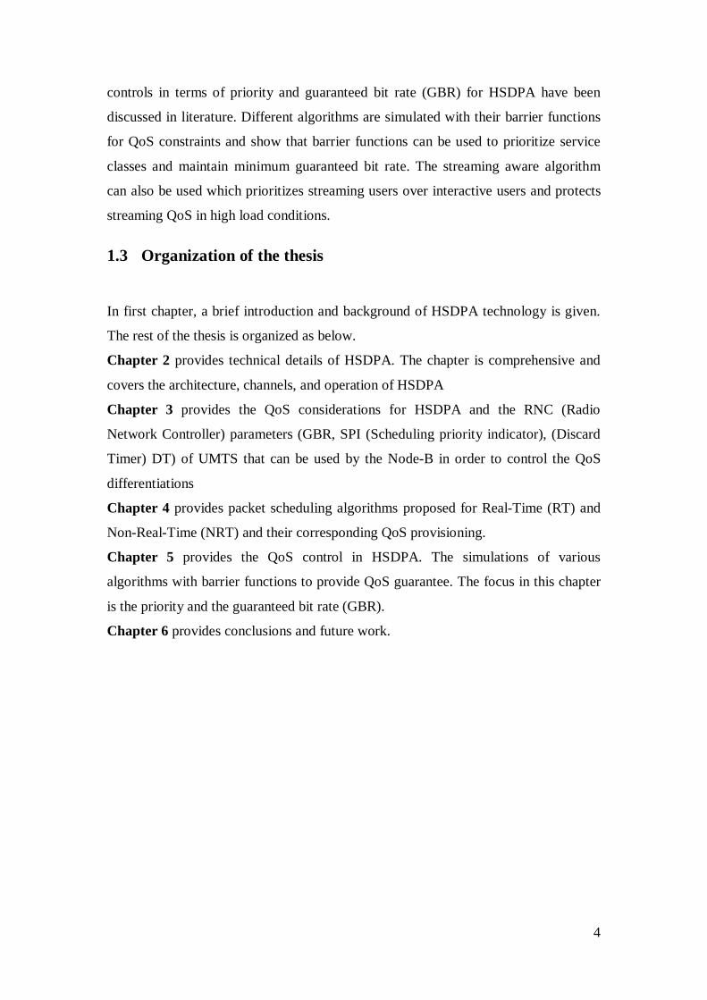
In HSDPA, each UE reports the channel conditions to Node B by means of CQI via

uplink physical channel (HS-DPCCH), shown in Figure 2.5. The CQI values are from

0 to 30 with a value 0 indicating “out of range”. Here Each CQI value corresponds to

a certain transport block size (column 2 in the following table), no. of HS-

PDSCHs(column 3 in the following table), modulation format, code rate and also data

rate and accordingly they are given an effective code rate. The CQI values and

corresponding TBS, HS-PDSC, modulation and data rates are shown in table 2.1

given below.

CQI

value

Transport

block size

(bits)

Number

of HS-

PDSCH

Modulation Data rate

(Kbps)

Effective

Code rate

0 NA NA NA NA NA

1 137 1 QPSK 58 0.14

2 173 1 QPSK 76 0.18

…………………………………………………………………………………… 27 21754 15 16-QAM 10866.5 0.76

28 23370 15 16-QAM 11674.5 0.81

29 24222 15 16-QAM 12100.5 0.84

30 25558 15 16-QAM 12768.5 0.89

14

Table 2. 1: CQI table for UE Category 10 [2]

The CQI value is entirely dependent on the signal to noise ratio (SNR) and HS-SCCH

signal receives that SNR which is discussed above. The selection of CQI value is

determined from the equation below.

≤

≤<+

≤

=SNR 14 30

14SNR 16- ]1.02

16.62 SNR[

-16SNR 0

CQI (2.1)

Where SNR is the “received signal to noise ratio” determined by the following

equation.

)10LIinter

10Iintra(101010.logTxP

TotalLTxPSNR

Total+

+−=

−=

(2.2)

• TxP is the transmitted code power in dBm.

• TotalL is the sum of distance loss, shadowing loss, and multi-path fading in dB

• Iinter is the inter-cell interference in dBm and it value ranges from -65 to -70

dBm.

• Iintra is the intra-cell interference in dBm which ranges from 30 to 35 dBm.

These values vary depending upon the scenario used. The transports block size,

number of HS-PDSCH, and modulation scheme determines the effective code rate.

The effective code rate can be calculated according to the following formula [5].

PDSCHHSbitsPDSCHHS#24TBsizeEff_code_

−×−+

=rate (2.3)

Where 24 is used as CRC (Cyclic Redundancy Check) in coding. The data rate can be

directly calculated from the transport block size divided by the transmission time

interval (TTI), which in HSDPA is fixed at 2ms:

15

2msTBSizeData_Rate = (2.4)

Many data rates are possible in HSDPA by varying the modulation type, effective

code rate, and number of multicodes.

Although there are 30 CQI values, still we have some 254 possible data rates i.e.

called transport block sizes for FDD mode (Frequency division duplex mode). There

are almost 2000 possible effective code rates (which means like we have almost 2000

combinations of the three parameters named: transport block size, number of HS-

PDSCHs, and modulation scheme) [5]

2.5 Hybrid Automatic Repeat request (HARQ)

Hybrid automatic repeat request (H-ARQ) is a physical layer error control technique

used in HSDPA. HARQ is the combination of feed forward error correction (FEC)

and ARQ. The ARQ scheme was previously used in UMTS Release 99. According to

the ARQ scheme, the received incorrectly data blocks are discarded and

retransmission occurs again. The stop and wait (SAW) Protocol was used to perform

ARQ procedure which means that the data block is transmitted. Then it waits for the

response before sending another new data block, or even for retransmitting of an

incorrectly received data block. However the scenario is a bit changed in HSDPA.

The retransmission is controlled by the new mechanism, HARQ, which is located in

Node B MAC-hs sub-layer. The unacknowledged data packets and the following

retransmission scheduling do not involve the RNC. Hence, there is no lub (interface

between RNC and Node-B) signalling between the RNC and Node B. That’s why the

retransmission delay of HSDPA is very much lower in comparison to the

conventional RNC retransmission used in UMTS.

The HARQ procedure is implemented in such a way that a wrong data block received

is not discarded but stored and soft-combined with the retransmission of the same

information bits. A HARQ process can be used for one block of data only at a time. It

takes around 5 sub-frames of time to receive the associated ACK/NACK response at

the Node B. This is known as single HARQ process. The disadvantage of this process

is the waste of latency time. To save latency time between the transmission of the

block and the reception of the ACK/NACK response, multiple independent HARQ

processes are used to transmit more than one block of data in parallel. The data rate to 16

a particular UE is thus increased and the available system capacity is not wasted. The

stop and wait procedure performed is the same as in UMTS and the same protocol

manipulates the given task.

Two different retransmission strategies are defined in 3GPP specification for

HARQ process; Chase combining (CC) and Incremental redundancy (IR). Chase

combining strategy defines that the retransmissions will be identical or the same as

the original transmitted data, while (IR) strategy tells that the retransmissions will be

different from the original transmitted data. With the (IR) scheme, if the decoding is

not successful at the first time then additional redundant information is transmitted

incrementally. Which strategy to be used? It basically depends on channel quality and

the UE capability class. The chase combing (CC) is more effective than the

Incremental redundancy (IR) when the effective code rate is high. On the other hand,

IR scheme is more efficient when the effective code rate is lower, but the flaw of the

incremental redundancy is that larger memory capacity is required by the UE.

2.6 HSDPA Packet Scheduling

Scheduling is the mechanism to determine which user to transmit data through

the shared channel (HS-DSCH) during a time interval TTI. The assignment of shared

resources to a specific user is of course an important decision. Therefore, scheduling

is the main soul in the design, as it determines the overall behaviour of the system.

There are some basis for scheduling decisions like channel condition, queuing delay,

and the priority of the UE. In HSDPA, Node B MAC-hs sub-layer is responsible for

making decisions (of UEs). It has been discussed in earlier sections that this

functionality is made near to air interface, i.e. Node B, to reduce delay and avoid the

signalling between RNC and Node B. This main feature in the HSDPA reduces the

delay as well as frame size (2ms). Above all, the scheduler should be such that it has

to grant equal time sharing among users, facilitate equal throughput to all users, and

maximize the total cell throughput.

Various scheduling schemes are based on traffic classes. These schemes are

categorized in two classes: Real-Time (RT) and Non-Real-Time (NRT). The

17

differentiation between these traffic classes are based on delays. The scheduling

schemes are not standardized by 3GPP but are vendor’s specific.

A simplified scheduling model is shown in the figure 2.7. It can be understood that

the flow control has control over the incoming packets, queued in the users queues,

scheduled, and send via physical channel(s).

Figure 2. 7: Node B scheduling model

2.7 HSDPA Operation principle

The simplified HSDPA operation principle is illustrated in Figure 2.8. The UE

measures the Signal to Noise Ratio (SNR or SIR) and periodically transmit the

channel quality indicator (CQI) on the uplink high speed dedicated physical control

channel (HS-DPCCH). This control channel also carries fast L1(level one) based

packet acknowledgement signalling (ACK/NACK) for each transport block. The

resources (codes, HS-DSCH power) are shared among users that are dependent upon

the estimated channel quality and the scheduling decisions. The Scheduling decision

are made in MAC-hs sub-layer at Node B and thus enables faster access to link

measurements, faster and efficient packet scheduling, as well as tighter QoS control

[13].

18

UE

Fast Adaptation is conducted in Node BBased on channel quality,QoS demands,

and ressource availability

HS-DPCCH (HARQ+CQI)

HS-DPCCH (HARQ+CQI)

UEHS-DSCH,HS-SCCH

Figure 2. 8: Simple illustration of HSDPA Operation principle [13]

The link adaptation is performed by (continuously) adjusting the modulation and

coding parameters every 2 ms TTI. The HARQ concept in HSDPA replaced the fast

power control used in UMTS and ensures the error-free detection with certain block

error rate (BLER). The Node B MAC-hs sub-layer handles the errors. When there are

certain errors occurring in the received data block, then the retransmissions are

performed by one of two strategies i.e. Chase Combining (CC) or Incremental

redundancy (IR). Buffers are used in the Node B to utilize the past retransmissions

that were received incorrectly. Due to the short delays it is possible to operate at the

1st transmission block error rate (BLER) values around 10-30 % [13].

19

Chapter 3

3 Quality of Service (QoS) in HSDPA Data communication has been the thrust and inspiration behind the development of

mobile wireless networks. The business growth of mobile communication market has

been dramatically increasing and can be considered as business opportunity of 21st

century. A variety of profitable and marketable services have been deploying by the

3G wireless networks operators. The industry need to develop the existing

infrastructure, end-user applications and network services toward an end-to-end IP

solution competent of supporting quality of service (QoS) to meet up the needs of the

prevailing data traffic [14].

From voice services to internet services anytime, and anywhere at mobile terminals is

the live example of the improvement and development of this technology and their

corresponding services. Providing services is not the main achievement of the

technology, but providing quality of service guarantees to applications for various

classes of services has become the main challenge for researchers.

This chapter is started with a short overview of UMTS QoS requirements and

its traffic classes. In the next section QoS consideration in HSDPA is discussed where

it is explained that how the UMTS parameters are used to differentiate the QoS

classes and the guaranteed bit rate (GBR). At the end, the QoS MAC-Aware

algorithm for the QoS control is presented.

3.1 UMTS QoS Requirements

As mentioned in earlier chapter, HSDPA is an evolution of the WCDMA and is an

extension of the existing 3G UMTS system. HSDPA QoS is based on the UMTS QoS

model. Thus it would be a useful idea to briefly discuss the UMTS QoS model and

their corresponding traffic classes. The standardization of UMTS QoS model started

in 1999 [01]. Release 99 distinct general QoS conscious bearer services which could

transmit IP real time traffic, like IP telephony. On the other hand, Release 2000

defined some more services that were left out in R99, like IP multimedia subsystem. 20

The main objective of the packet service QoS standardization for UMTS is to provide

data delivery with suitable end to end QoS guarantees. According to [3] there are

three types of Quality requirements in UMTS. 1. End User Requirements for QoS: Only the QoS perceived by end-user matter.

The number of user defined parameters should be smaller.

Derivation/definition of QoS attributes from the application requirements has

to be simple.

QoS attributes must be able to support all applications used, a firm number of

applications are having asymmetric characteristic in nature between two

directions, uplink/downlink.

End-to-End QoS has to be provided.

2. General Requirements for QoS QoS should be competent of as long as dissimilar levels of QoS by using

UMTS precise control mechanisms.

QoS mechanisms have to use radio capacity efficiently and effectively.

Allow autonomous evolution to Core and Access networks

3. Technical Requirements of QoS

UMTS QoS mechanisms must present a mapping between application needs

and UMTS services.

UMTS QoS mechanisms must be able to resourcefully interwork witht QoS

schemes.

QoS must support competent resource utilisation.

QoS parameter are needed to bear asymmetric bearers.

QoS performance should be dynamic, i.e., it should be possible to modify QoS

parameters while an active session.

The main objective of the packet service QoS standardization for UMTS is to provide

data delivery with suitable end to end QoS guarantees. 3GPP has proposed some

21

layered architecture for the UMTS to specify the data delivery with suitable QoS end-

to-end. Layered architecture model of UMTS shown in fig 3.1.

Figure: 3.1 UMTS QoS Architecture [3], [16]

The description of QoS in layered architecture requires attributes for each bearer

service indicated. In order to map such attributes serve end to end QoS requirements

for each bearer service worn by data connections [1].

The connectivity from one UE to another UE passes through different bearer services.

These services are summarized below.

TE/Local bearer services (Communication between different components of

mobile station like laptops or traditional mobile phones).

UMTS bearer service (comprises of Radio access bearer (RAB) and Core

network (CN). RAB is responsible for transporting signalling and user data

between the UE and Core network, while CN connects with core network

gateway to the external network and is responsible for efficiently control and

utilization of backbone network).

The exterior local bearer service (UMTS core network connected to the

destination node located in an external network).

22

UMTS offers end-to-end connectivity via

1. Circuit switching (CS) with (PSTN) public switched telephone network and

integrated services digital network (ISDN).

2. Through packet switching (PS) domain IP connectivity.

Unlike the previous technologies UMTS will be supporting asymmetric traffic

bearers, i.e., the bit rate, which is the major attribute in QoS, can be different in uplink

and downlink direction. This will ultimately deliver a proper and effective utilization

of the available bandwidth. For example if the bearer is used for some applications

like streaming video, the bit rate in one direction is less than other. Following are

various QoS attributes.

1. Maximum bitrate (kbps): UMTS delivered maximum number of bits and UMTS at

a SAP within a time period, dividing by the period duration.

2. Guaranteed bitrate (kbps): UMTS convey certain number of bits at SAP within a

time period, dividing by the period duration.

3. Delivery order (y/n):it tells if the UMTS bearer shall provide in-sequence SDU

delivery. The Transport Network Layer is supposed to transport the packets in

sequence to the peer entity.

4. Maximum SDU size: the maximum allowed SDU size.

5. SDU format information (bits): list of possible exact sizes of SDUs.

6. SDU error ratio: it tells fraction of SDUs loss or found as errors. SDU error

proportion is distinct for conforming traffic.

7. Residual bit error ratio: it tells the hidden bit error ratio in the delivered SDUs.

Residual bit error ratio tells the bit error ratio in the delivered SDUs when no error

detection has been asked.

8. Delivery of erroneous SDUs (y/n/-): it tells that if SDUs detected as erroneous

should be delivered or spared.

9. Transfer delay (ms): It tells maximum delay for 95th percentile of distribution

delay for every delivered SDUs during the life span of a bearer service, where delay

for an SDU is the time for a request to deliver an SDU at one SAP to other.

10. Traffic handling priority: it explains the importance for conducting of all SDUs

related to the UMTS bearer compared to other bearers.

23

11. Allocation/Retention Priority: it explain the significance compared to other UMTS

bearers for allotment and preservation of the UMTS bearer.

The attributes definition of the TE/ Local bearer service and \outer bearer is outside

from the scope of current standardization for QoS within 3GPP [11]. But UMTS

attributes and access bearer service of radio is described by the current specification

in 3GPP QoS standardization. The UMTS important bearer attributes are given in the

following table.

Traffic Class Conversational Class

Streaming class

Interactive Class

Background Class

Maximum Bit rate.

* * * *

Delivery Order * * * * Maximum SDU Size

* * NA NA

SDU Error Ratio

* * * *

Transfer Delay * * NA NA Guaranteed bit rate

* * NA NA

Traffic Handling priority

NA * NA NA

SDU Format Information

* * NA NA

Residue Bit rate * * * *

Table 3.1: UMTS bearer attributes for each traffic class [16]

Some of the attributes are irrelevant for some traffic classes. For example the

maximum SDU size is inappropriate for interactive and background class.

24

3.2 UMTS QoS Traffic Classes

According to [4], “an application is defined as a task has the requirement to

communicate information streams at least one, between two or more systems which

are at different geographical locations.”, while Service is classified as a combination

of applications with alike characteristics. Depending on classification criteria, there

are many ways to categorize services, such as the directionality (unidirectional or bi-

directional), symmetry of communications (symmetric or asymmetric), etc. The 3GPP

has a traffic Classification which separates types according to general QoS

requirements. The QoS is the combined result of service performances that decide the

degree of approval of the end-user of the service. 3GPP has specified 4 different QoS traffic classes. These classes are based on the

traffic delay sensitivity with reasonable QoS resolution.

There are 4 QoS classes:

• Conversational

• Streaming

• Interactive

• Background.

The difference between the classes is delay sensitivity with the traffic. Conversational

class is intended for traffic very delay receptive. On the other hand background class

is the least delay sensitive class [4]. The conversational and steaming classes are

proposed to take real time traffic like, video telephony and are useful for the most

delay sensitive applications. On other hand background classes are labelled as non

real time traffic classes like the interactive class is used to clutch traditional internet

traffic such as WWW, email, while background traffic class is used for file transfer

applications like FTP. The detail description of each class is given below.

• Conversational Class

This class is considered as the most delay sensitive and the known example of is

telephony speech i.e. GSM but as the internet and multimedia is progressing a number

of new applications require this class like Voice over IP (VIOP) and video

conferencing. The real time discussion is always occured between peers or group live

(human) end user that’s the reason this is class is reserved for the real conversation.

25

Basically, HSDPA is considered mainly for streaming and downloading. That is the

reason it does’t deal that much with conversational class.

Because of the nature of the class, real time conversational class is characterized by

the low transfer time. The variation of time between in series entities of the stream is

summarized in the similar way for the real time stream. Maximum transfer delay is

the end to end user’s perception of video and audio conversation. Hence, the limit of

delay is very severe, failure provides low enough that delay transfer will result in lack

of quality. Requirement for transfer delay is significantly lower than the round trip

delay. End to end belonging to this class should not exceed 150 ms.

• Streaming class

This class is designed to support real time video streaming. The data flow of this class

is considered as one way transport. This kind of traffic is more delay tolerant than

conversational class. The end to end delay variation flow shall be limited to a certain

limit. It does not have any strict delay requirements. The stream is normally aligned

with time at the receiving end; therefore the maximum suitable delay difference over

the transmission media is the time alignment function of that application.

As they can tolerate larger delays because of there non-interactive nature and for this

reason the network is allowed to delay the straming packets. According to [2], today’s

streaming applications apply time alignment prior to decode at receiving end. The

time placement function at first delays by buffering the received stream before

starting the decoding process which enables to cope with the delay variations in

accordance with the buffering capabilities limits. This is also real time service class.

• Interactive Class

The interactive class is non real time communication where the end user requests

online data from remote equipment. This kind of traffic class is not delay sensitive

and represents bursty traffic. Example of this class is human interaction with the

remote equipment like web browsing server and telnet.

26

There are two properties of this traffic class. [11]

1. One of the key properties of interactive class is the response time. The

message sent to the destination is expected to be reached within certain time which

defines the degree of satisfaction.

2. Another key property of this class is the contents of packets to be transferred.

• Background Class

Background traffic class is another kind of non real time class where the

communication is performed by machine to machine data transfer. It is the most

insensitive delay traffic class with least error rate. Typical example of this traffic class

is the delivery of Emails, SMS, FTP files, etc.

Background traffic is the classical data communication schemes where data are not

expected to be received in an exact time unlike the interactive traffic class. Another

key feature of background class is that the stuffing of the packets shall be clearly

transferred like interactive class [11]. The table given below table shows a short

overview of the above discussed UMTS QoS traffic classes.

Traffic Class Conversational Class

Conversational RT

Streaming Class

Streaming RT

Interactive Class

Interactive Best effort

Background

Background best effort

Fundamental Characteristics

- time relation preserves in between the information entities of the stream

- conversational pattern

-time relation preserve between information entities of the stream

Request Response pattern

Preserve payload content

Destination data expectation at a certain time

Preserve payload content

Example of the Application

- voice - video streaming -web browsing -background emails downloading

Table No. 3.2 UMTS QoS Classes [3]

3.3 Real and Non Real Time Traffic:

Traditionally, classifying services presence to their delivery requirements, they

have been primarily divided between Real and Non Real Time services. Usually, Real

27

Time (RT) services have been considered to impose strict delay requirements on the

end-to-end communication, so that any of the network nodes concerned in the Real

Time connection is to transfer the packets of the RT flow within a maximum average

delay. Due to these severe delay constraints, there are only little chance of error

correction, while link level retransmissions are hardly appropraite for Real Time

services, end-to-end recovery mechanisms have been completely dismissed. This

shows the real time flow at the end entity depends on transmission errors, and the

final application must deal with these errors.

Still, Non Real Time traffic has been commonly considered as error sensitive, though

not that much demanding as RT traffic constraints. One other classic difference

between RT and NRT services is that the receiving end of RT applications usually

gets through the information before the end of the data transaction.

The 3GPP QoS specification also follows the RT/NRT classification by identifying

the conversational and streaming traffic (Real Time services), whereas the interactive

and background services are claimed to respond to a Non Real Time traffic. When

some delay delivery requirement are set on background and interactive users then

there is a little difference left with Real Time services [2] like Network gaming. The

remaining of the thesis will still assume the division between NRT and RT traffic.

Those services will be considered as NRT whose payload must be transferred error

free, and whose transmission delay requirements allow for end-to-end error recovery

mechanisms such as carried out by the Transmission Control Protocol (TCP). In

contrast, Real Time services will be considered as those whose transmission delay

requirements do not permit end-to-end retransmissions mechanisms, and transferred

by unreliable transport protocols such as the User Datagram Protocol (UDP).

3.4 QoS Considerations for HSDPA

According to [7], there are basically three mechanisms that can be used to implement

HSDPA QoS control.

1. Dynamic allocation of transmission resources for HSDPA

2. Quality based HSDPA access control, and 28

3. QoS aware MAC-hs packet scheduling.

a. Dynamic allocation of broadcast resources for HSDPA includes the

power and channelization codes that the MAC-hs is usedfor transmission.

The canalization codes are relevant for cells where the available power

and channelization codes for each cell are shared involving Release 99

dedicated channels and HSDPA.

b. Quality based HSDPA access control algorithms decide whether a

new HSDPA user should be granted/denied access, depends on the QoS

requirements and the current load in the cell.

c. Finally, QoS aware MAC-hs packet scheduler is responsible for

scheduling the admitted users on the shared data channel so their QoS

requirements are fulfilled.

While designing the QoS for HSDPA, the functional split between RNC and Node-B

must be carefully considered. The scheduler is positioned in the Node-B rather than

RNC as it was in release 4. In this way, the delays for the scheduling process are

minimized [4]. The standardized interface between RNC and Node-B controls the

QoS for HSDPA through some measurements and parameters. The architecture and

functional split between RNC and Node-B is shown in figure3.2.

Figure3.2: Functional split between RNC and Node-B and UE for HSDPA [6]

29

The architecture consists of three parts: RNC, Node-B and UE. The RNC consists of

user-plane protocol stack and the primary Radio Resource Management(RRM)

algorithms. The following are the functions of RRM at the RNC:

Hanover

Quality Based HSDPA access control

Setting of specific HSDPA QoS parameters and,

Allocation of HSDPA transmission resources (Power and Channelization codes) to the MAC-hs.

The RNC provide guidance to the MAC-hs in Node-B how it should schedule

each user while on the other hand Node-B provides feedback measurements to the

RNC for the monitoring the performance of air interface. Because once a HSDPA

user has been allocated RNC is then not aware of how often the MAC-hs scheduler

in Node-B schedules the user and the instantaneous data rate given to the user in

each served TTI. But Node-B gives the feedback.

QoS-aware packet scheduling for Release 99 dedicated channels is a function of the

user’s traffic class, traffic handling priority, allocation retention priority (ARP) and

other UMTS bearer attributes. However, the TC and THP are not available in the

Node-B for MAC-hs packet scheduling in HSDPA. Therefore a new QoS interface

was defined for HSDPA between the RNC and Node-B [11]. Figure 3.3 shows an

overview of the HSDPA specific QoS parameters.

Figure 3.3: HSDPA QoS interface between RNC and Node-B 3GPP specifications: 25.214 and 25.433

30

The guaranteed bit rate (GBR), scheduling priority indicator (SPI), and Discard Timer

(DT) can be used to guide the performance of MAC hs Scheduler. The GBR can be

set for a user with minimum target bit rate while the SPI can be set to give priority to

data flow to achieve that target. The SPI has integer values from 0-15; the high value

shows the high priority while the lower value shows the lower priority. The DT is the

maximum time a packet can be in the buffer of Node-B MAC-hs before it should be

discarded. The SPI and GBR are the two primary parameters that can be used to

control the QoS differentiations on HSDPA. The GBR, SPI and DT can be set by

manufacturer or operators according to the TC and THP. The table is illustrated in

below

Traffic Class GBR SPI DT

Streaming X X X

Interactive THP=1 X X X

THP=2 X X X

THP=3 X X X

Background X X X

Table 3.3: Mapping of HSDPA QoS parameters [7]

For example mapping of VOIP services to interactive TC with THP=1 with GBR=16

kbps and using a high SPI worth to indicate that voice services should be given high

priority, similarly for streaming TC, the HSDPA GBR parameter can be set to the bit

rate requirements.

RNC is updated with some measurements regarding HSDPA power as shown in the

figure 3.4. If RNC does not allocate any HSDPA transmission power, the Node-B can

use unused power available in the cell for HSDPA transmissions

3.5 QoS Aware MAC-hs Packet Scheduling

The available HSDPA capacity depends on the allocated users and the variations of

the radio channel conditions. Figure 3.4 shows the availability of HSDPA cell

capacity, the required capacity, and the excess capacity.

31

Figure 3.4 HSDPA cell capacity, excess capacity, and required capacity [7]

The required capacity is the total capacity needed to serve all the owed users at their

GBR, while the excess capacity is the remaining capacity up to total available

HSDPA cell capacity. The feasible region is defined as “the region where the given

capacity is at least equal to the required capacity”. When the available capacity is

smaller than the required capacity, then the MAC-hs scheduler can’t schedule users at

their GBR. This is knows as congestion. Assuming that system is functioning in the

feasible region, the excess capacity could be distributed among the allocated users

according to SPI parameters. A hard prioritization strategy could be followed to give

the available capacity to users with highest priority (highest SPI), followed by the user

with second highest priority. The benefits are given to those users with highest

priorities while others are given only the GBR.

Another approach can also be used which is known as soft prioritization

strategy. This strategy states that a large fraction of available capacity is given to

highest priority users as compared to other users with lower SPI priority. A hybrid

solution of hard and soft prioritization is also possible. The strategy could be

implemented as the hard prioritization strategy can be used for high SPI i.e. SPI=15

while soft strategy could be used for other users with lower SPIs. By implementing

this strategy, the users with SPI=15 will first use all the excess capacity until no data

are buffered in Node-B for those users, followed by the remaining capacity by other

users.

The 3GPP specifications do not specify the required behaviour of MAC-hs scheduler

according to the SPI settings for the allocated users. The Node-B manufacturers and

the operators can select the suitable solution. The MAC-hs scheduling algorithm can

32

be designed by the general mathematical utility function in [12] for each user

depending on its GBR and SPI.

Given the utility function (.)nU , the scheduling metric for user n can be defined as

n

nnnn r

rURM∂

∂=

)( (3.1)

Where nR is the instantaneous data rate and nr is the average data rate. The MAC-hs

scheduler selects the users with highest scheduling metrics as

}max{)(Pr ni Mn = (3.2)

A well-liked algorithm with minimum guaranteed bit rate constraints proposed in [12]

is implemented with the same approach explained above as for GBR as

[ ]))(exp(/1 nnnnn GBRrrdM −−+= βα (3.3)

The parameters α and β control that how the scheduling priority of user should be

increased. A more detailed description and simulations of this algorithm is given in

next chapter.

In conclusion, Klaus I. Pedersen [12], [14], and [15] demonstrated how the QoS

parameters for UMTS can be re-mapped in the RNC and can be used as QoS

parameters for HSDPA that can communicate to the Node-B packet scheduler. Klaus

I. Pedersen also proposed Quality based HSDPA Access Algorithm in which the

algorithm is capable of controlling admission of new users based on transmission

power without violating the GBR of allocated users.

33

Chapter 4

4 Packet Scheduling in HSDPA HSDPA represents a new Radio Access Network concept that introduces new

adaptation and control mechanisms to enhance downlink peak data rates, spectral

efficiency and the user’s Quality of Service.

Wireless link capacity is usually a rare resource which should be used efficiently.

Therefore, it is important to find competent ways of supporting QoS for real-time data

(e.g., live audio/video streams). Enough capacity is required which can support the

maximum possible users with the desired QoS. For addressing this issue efficient data

scheduling is one of best ways. [17].

The HSDPA enhancing characteristics and also the location of the scheduler in the

Node B creates new potential chances for the design of this functionality which can be

used for the development of WCDMA/UTRAN. The goal for the Packet scheduler is

to maximize the throughput according to satisfactory conditions of QoS of the users.

Therefore HSDPA scheduling algorithm, for enhancing the cell throughput, can use

the instantaneous channels variations for its advantage and thus the priority of

favourable users can be increased temporarily. Since the quality of user’s channel has

asynchronous variations, the time-shared nature of HS-DSCH introduces a kind of

selection diversity. This introduction will also give benefits for the spectral efficiency.

The QoS requirements of the interactive and background services are the least

demanding of the four UMTS QoS classes, and have been generally regarded as “best

effort traffic” and no guarantees are provided in these services. As commented in

Chapter3, the UMTS bearers do not set any absolute quality guarantees i.e, in terms of

data rate for interactive and background traffic classes. However, as also stated in

Chapter 3, the interactive users still expect the message within a certain time, and for

it all users should be given access but could not be fulfilled if any of those users were

starved of access to the network resources. Additionally, as described in [4], the

starvation of NRT users could affect the performance of the high layer protocols, like

TCP. Therefore the introduction of minimum service guarantees for NRT users is a

34

related factor. The service guarantees interact with the idea of fairness and also the

satisfaction level among users. In the very unfair scheduling mechanisms the least

favourable users will me most probably starved in high loaded networks. The above

all concepts and their effect on the HSDPA performance are to be discussed in this

chapter.

4.1.1 Real-Time-Packet Scheduling Schemes Utilization of wireless channels is one of the challenging topics for researchers. As

discussed in the previous chapter the issue is not to provide service to the users but

infact to provide the service with the desired efficiency and quality that is desired to

them. As the Quality of a wireless channel changes instantaneously for different users

with time and the efficient usage of the resources is one of the most difficult assigned

tasks in wireless networks. It becomes more difficult when there are some limitations

like delaying packets and maintaining a specific data rate as required in real time (RT)

applications such as VoIP and video streaming.

Taking these considerations into account and to provide the desired QoS for the real

time applications, some of scheduling algorithms can solve it which are presented

below. Before starting with scheduling algorithms, the following notations are defines

below.

• )(Pr ti is the priority assigned to user (i) of time t ,the user with highest priority is scheduled.

• t is the Transmission Time Interval (TTI).

• )(tRi is the instantaneous data rate of user (i)

• )(tiλ is the average throughput of user (i) at time t

• )(tiW is the “queuing delay” experienced by the head of line packet of flow (i) at Node B

4.1.1.1 Modified Largest Weighted Delay First (M-LWDF) Andrews [17] proposed the M-LWDF algorithm for real time data users. This

algorithm states that the probabilities of the delay of the data packets needed be at

least below a certain threshold value.

35

The priority is given to the user (i) at a time t is as follows.

iTtiW

ti

tiRiati

)(.

)()(

)()(Prλ

= (4.1)

Where ia represents the QoS parameter that can be used for differentiation of

different users with different QoS requirements such as traffic classes or end to end

delay. The QoS of user (i) can be determined from the following formula.

iiTiW δ<> )Pr(

Where iW is the packet delay for that user, iT is the certain threshold value, and iδ is

the maximum probability with which the system is given the right to violate the delay

requirements. The lower value of iδ corresponds to the lower probability of

exceeding the packet delay of that user. According to 3GPP Technical Specification

25.858, M-LWDF algorithm is unfair and unable to perform well during bad radio

conditions means it gives priority to the UE’s in feasible range. Similarly, another

problem is that when the priority is equal to zero i.e. iW =0, then all the SDU’s

(Service Data Unit) have to wait until the priority is increased. This wait is called the

intrinsic delay which can be experienced by each SDU.

4.1.1.2 Expo-Linear (EL) Some other algorithms have been proposed in the literature to avoid this intrinsic

delay. One of them is the Expo-Linear algorithm. This algorithm prioritizes users

according to the following formula. [21]

))(exp()()(

)()(Pr tiWiati

tiRiati λ

= (4.2)

All the parameters are same as for M-LWDF like QoS parameters, delay etc but this

algorithm introduces exponential term that’s why it is known as expo linear

algorithm. When the delay is low, the Proportional Fair algorithm dominates the

scheduling decision but when the delay is high or approaches to delay bound the

priority increase in an exponential manner accordingly [21]

4.1.1.3 Exponential Rule (ER)

36

Exponential Rule (ER) scheduler has been proposed for real time applications. The

users are prioritized according to the following formula.

aW

WatiWiatirtiR

iati+

−=

1

)(exp.

)()(

)(Pr (4.3)

Where ∑= i tiWiaN

aW )(1

ia Represents the priority values given to the different QoS classes and N is the

number of users. This algorithm consists of two parts. The earlier part )()(

trtR

i

i

represents the PF algorithm used for non real time (NRT) applications which could be

discussed in more details in next sections while the second part is the exponential part

which describes the delay of the user (i). If the exponential term is close to one then

this algorithm behaves as Proportional Fair (PF) algorithm. On the other hand, if one

of the queues would has a larger (Weighted) delay than the others by more than

order Wa , then the priority is given to that user (i). The factor 1 in the denominator of

the rule is present only to prevent the exponent from blowing up to infinity when the

delays are small.

4.1.1.4 Modified Proportional Fair (MPF) The Modified Proportional Fair (MPF) algorithm has been proposed for Real time

applications in [20]. This algorithm prioritizes the users according to the following

formula.

{ }τ

τ

≥

<

=

iWtiR

tjRjtirtiR

iWtirtiR

i,

)(

)(max.

)()(

,)()(

Pr (4.4)

Whereτ denotes the certain threshold for delay dependent QoS class, { })(max tR jj

represents the maximum average supportable data rate or maximum average CQI

report value from all the users, while )(tRi indicates the average supportable data

rate of user (i)

37

This algorithm is proposed for the video data flow which prioritizes the users based

on the delay. This algorithm also contains two parts. The 1st part is a simple

Proportional Fair algorithm. When the delay is lower than a certain threshold valueτ ,

the algorithm behaves as Proportional Fair (PF) and prioritizes the users according to

the formula given in the first part of the equation given above. But when the delay is

higher than that certain threshold for users, then users are prioritized with the second

part of the algorithm. The aim of this second part with some modification is that it

gives equal throughput to all of the users.

4.1.2 Non-Real-Time (NRT) Packet Scheduling Schemes Non Real Time (NRT) traffic is commonly considered as error sensitive and delay

insensitive. The scheduling schemes designed for this kind of traffic class is

considering bursty traffic. The UMTS QoS classes include interactive and background

classes as discussed in chapter 3. These kinds of classes do not require any QoS

guarantee. However for the interactive class users, certain amount of time is fixed to

receive the message. The aim of these scheduling schemes are considering good

quality channel condition (better CQI) and prioritize users to get maximum

throughput while maintaining the fairness. There are some NRT scheduling schemes

proposed in literatures which are discussed below.

4.1.2.1 Round Robin Algorithm Round Robin Scheduling algorithms serve users in a cyclic order. The queues that

have no data are skipped so that the time slot will not go wasted. The number of

parallel HS-PDSCH, modulations and coding schemes, and transport block size

depends on the reported channel quality conditions of the users. Round Robin scheme

provide equal time to all users. It does’t offer any priority to UE’s.

4.1.2.2 Maximum Signal to interference noise ratio (max CIR) This algorithm is proposed in [21] and schedule users with best channel quality

condition in every TTI. The users are prioritizing according to the following formula.

)}(max{)(Pr tRt ii = (4.5)

38

Where )(tRi is the instantaneous data rate experiences by the user (i). The main

drawback of this scheduling algorithm is that when the user is away from the Node B

and have bad channel condition, the user will never be scheduled.

4.1.2.3 Proportional Fair (PF) This scheduling scheme has been proposed in [22] for HDR (High Data Rate). This

algorithm tends to allocate data rates fairly to different users. The users are prioritized

according to the following formula.

)()(

)(PrtrtR

ti

ii = (4.6)

This algorithm tends to serve users under favourable instantaneous radio channel

condition and allocate resources to their users proportionally fair. The disadvantage of

this algorithm is that it serves users with lower throughputs which get favourable

channel condition. Thus it can be said that this algorithm is not throughput optimal. It

is mentioned in [19] that the proportional fair algorithm does not account for delay of

packets and can result in poor delay performance and thus cannot be used for QoS

differentiations. In next chapter it will be proved that this algorithm cannot account

for delays.

4.1.2.4 Fast Fair Throughput (FFT) This algorithm has been proposed in [20] to provide balance throughput and fairness

among all the users. This algorithm is the modification of the proportional fair (PF)

algorithm. The users are selected at every TTI, according to the following formula.

{ }

=

)(

)(max.

)()(

)(PrtR

tRtrtR

ti

jj

i

ii (4.7)

{ })(max tR jj , represents the maximum average data rata from all users while )(tRi

indicates the average supportable data rate of user i. As seen from the formula that the

first part is PF algorithm and on the other hand the second part of the formula is used

for the distribution of thethroughput among all the users. The addition of )(tRi term

39

in the denominator increases the priority of that user which has less favourable

channel condition and thus tries to distribute the throughput fairly.

4.1.2.5 Throughput Guarantee Scheduling (TGS) The focus of TGS algorithm is to offer a minimum throughput with a certain outage

probability to all the users that can maintain the QoS requirements. The proposed

algorithm is known as Throughput Guarantee Scheduling (TGS) [23]. The throughput

outage probability of the user (i) is defined as “the probability that the throughput of

user can not satisfy the required target throughput” which is articulated as follows.

ireqiii TT δ≤< )(Pr ,

Here, iT represents the average throughput and reqiT , is the required minimum

throughput of the user (i). iδ is the required target throughput outage probability of

user (i). The proposed algorithm [23] is a modified version of Proportional Fair that

can maintain the minimum throughput requirements of a user and can guarantee the

QoS. The users are prioritized as follows

<

<

=

reqiii

i

reqiiTT

ii

i

iTifT

ttR

TifTCttR

t

reqi

,

,/

)()(

.)()(

)(Pr

,

λ

λ { })(

)(maxtR

tRC

i

jji = (4.8)

where { })(max tR jj is the maximum average data rate of the system and iC is the

extra weight which increases the users throughput if they are having too low

throughputs to meet the QoS requirements. reqiTT ,/ is the normalized throughput of

user (i). If the user throughput is close to the require target throughput, the

exponential term becomes close to 1 and therefore gives the high priority to users who

can easily achieve their target throughput which maximize the number of satisfied

users [23].

40

Chapter 5

5 System Model and Simulation Results Various scheduling algorithms have been proposed to schedule users over a shared

link. Some of them provide QoS guarantee and relatively complicated to implement

while others might be simple but cannot provide QoS guarantee. Some of the

algorithms proposed in the literature can be considered to maintain the simplicity and

QoS guarantees by taking advantages of channel conditions. The schedulers try to

provide the user QoS demands of each connection and tries to maximize throughput.

In this chapter the system model is given. At first the barrier function for QoS control

are presented. The QoS differentiation is performed by barrier functions. The chapter

is started with a short overview of the barrier function and then the methodology to

differentiate between traffic classes is explained. The traffic classes are differentiated

and then simulated them to study the QoS guarantee with their minimum Guaranteed

Bit Rate (GBR). In the next section application of HSDPA are discussed and

streaming and interactive users with their GBR are simulated. A model is presented

for interactivec services in [30], to satisfy the required QoS. Then different algorithms

are discussed where traffic classes are differentiated by means of delays. At the end,

the chapter is summarized with some conclusions.

5.1 Barrier Functions for QoS Constraints The barrier function has been proposed in [24] in order to provide QoS guarantees

also and to take advantage of user diversity gains. As discussed in this section

3.3.2.2; the users with good channel condition are picked by the Maximum Singnal to

Noise Ratio(Max SNR) and thus maximizes the throughput. The barrier function

introduced can be used with the max SNR algorithm to maximize sector throughput.

The minimum throughput for a particular connection is maintained by the utility

function as

)1()( )( minrrerrU −−++= β (5.1)

41

where minr is the minimum throughput and β is the penalty parameter which

determines the rate at which the penalty is increased for violating the constraint.

When the throughput exceeds the required minimum value the function behaves as

max SNR which was discussed in the section 3.3.2.2. But when the value of r drops

below the minimum value, the scheduler selects the users which are below the

minimum value and thus maximize the throughput of those users. The service classes

are classified according to the β value and the barrier function performs a barrier

around the feasible region.

A quadratic barrier function is used as the utility function. It will impose penalties

when moving away from the desired CSE (Circuit Switch Equivalent) rate. Two types

of classes are considered via simulating the proposed algorithm. The first one of them

is Gold users where the Circuit Switch Equivalent (CSE) is kept at 128 kbps and the

other is Silver users where the Circuit Switch Equivalent (CSE) is set to 64 kbps. The

primary utility function used is the max SNR function. The utility function is given by

the equation 5.2 below. 2)()( CSErrrrU −−= β (5.2)

Where β determines the degree of the QoS demands. The value of β for Gold users

is β =0.03 while β =0.02 for Silver users. The scheduler chooses the users by the

following formula.

[ ])})((21)(max{)( CSErnjrnjdnrP −−= β (5.3)

)(nd j is the instantaneous data rate of the user and )(nrj is the user throughput

which can be assumed as exponentially smoothed user throughputs and can be

computed by the following equation.

+−

=+Otherwise )()r1/-(1

nslot in served i )(

)()/11()1(

i n

ifnd

nrnr

ii

jτ

ττ

(5.4)

Where )(ndi the bit rate of user (i) is,τ is the time constant for the smoothing filter,

the value of which is kept 10 and )(nri is the average throughput. As long as the

42

resources are available all the users will achieve the desired CSE throughputs and will

provide QoS guaranteed.

The above discussed scheduler is simulated. A simple Matlab based model is

presented below to simulate the barrier functions.

1. SNR Generation

The SNR values are being generated from one of the popular path loss model known

as Okumura Hata Model (COST 231). This model is given by the following formula .

ERBFdBL −+= 10log)( hbfF c 1010 log82.13log9.333.46 −+= (5.5)

B= hb10log55.69.44 − E= 2

10 ))7554.11((log2.3 R=1km where cf represents the carrier frequency which is set as 2100 MHz , hb denotes the

base station antenna height set to 30 meters and R represents the distance between

Base station and mobile station. The value of hb is set to one Km in our model. In

the model shadowing and noise are also came under consideration. The readers are

encouraged to read the matlab code for Okumura Hata Model including shadowing

and standard deviation in Appendix. The following formula generates the SNR

values.

SNR = noiseModelOkomuraTx p −− _ (5.6)

where the pTx denotes the transmit power of Node-B which is 16 watts for HSDPA

and the noise is )2(log10 1210

−×= enoise . The generated SNR values are shown in Figure 5.1. The values range from -30 dB to

30 dB. The SNR values greater than 10 dB are considered as good quality signal.

Figure 5.1 below represents the generated SNR values versus number of users.

43

Figure: 5.1 SNR versus Users

2. Mapping of SNR into CQI

The SNR values generated from Okumura Hata Model are then mapped to the CQI

values according to the equation mentioned in [9].

≤

≤<+

≤

=SNR 14 30

14SNR 16- ]1.02

16.62 SNR[

-16SNR 0

CQI (5.7)

The CQI values are sent by the uplink channel HS-DPCCH. 3GPP defines the

transport block size corresponding to CQI values. Detail description is given in

chapter 2.

44

3. Mapping of CQI into Data rates

The CQI values are then mapped into data rates which is described in the 3GPP

specification[2]. The 3GPP mentions the data rates corresponding to CQI values both

with 10% Block Error Rate (BLER) as well without BLER. In our model, we have

mapped the data rates corresponding to CQI values without (10%) BLER Figure 5.2

represents the mapped data rates versus number of users.

Figure 5.2: Data Rates versus Users

5.1.1 Max SNR and Proportional Fair Algorithms The Max SNR and Proportional Fair algorithm used with quadratic Barrier Function

proposed in [24] is the primary function to be used. Before starting with this

algorithm, first of all, simulation of the max SNR and Proportional Fair algorithms is

carried out to make a primary function for the mentioned barrier function. The

algorithms are simulated for simulation times of 700 seconds having 10 users in a

cell. Figure 5.3 shows the simulated combined result of the max SNR and PF

algorithm. The figure confirms that the max SNR maximizes the throughput by

selecting users with the favourable channel quality conditions while the PF algorithm

45

serves users with lower throughputs as the behaviour of this algorithm is that it serves

users proportionally fair. The SNR algorithm is fruitful for those users who are closed

to the Node-B and enjoy good SNR values. The bad quality signal users are starved

and thus the resources are not shared equally among the users.

Figure 5.3: Simulation of max SNR and PF algorithms

5.1.2 Barrier Function with max SNR In this section the barrier function is used with max SNR. The max SNR function is

the primary function in the simulation of this algorithm. Gold users are given priority

over Silver users through the Barrier function. The simulated results are quite

reasonable and show that this Barrier Function can differentiate between different

kinds of traffic classes while providing the QoS guarantee. The immense important of

this barrier function is that it enforces QoS constraints. Figure 5.4 shows the

differentiation of Gold and Silver users. There are 20 users in total of which 10 users

are Gold users while other 10 users are Silver users. The aggregated data rates for

Gold as well Silver users can be seen from the Figure 5.4. Here the Gold users are still

given priority to satisfy QoS guarantee. It can be observed from Figure 5.4 that the

46

reduction in data rates of the Gold users is due to the penalty function which implies

satisfaction to both of the traffic classes for their minimum QoS requirements.

Figure: 5.4 Barrier Function with max SNR

The max SNR algorithm, Proportional Fair alone as well as max SNR with Barrier

Function are simulated to see how the cell throughput is decreased when these

algorithms are used with Barrier Function. The result shows that cell throughput

decreases when the barrier function is used. On the other hand, the barrier function

satisfies the users for their minimum required bit rate. Figure 5.5 shows the

comparisons chart below.

Comparisions of Cell Throughput for Algorithms alone and Algorithms with Barrier Function

10

8

3 2.5

0

2

4

6

8

10

12

Cell

Thro

ughp

ut (M

bps)

Max SNRPFSNR_GoldSNR_Silver

Figure: 5.5 Comparisons of algorithms with barrier function

47

Now simulation are performed for one user each traffic class. When only one user is

simulated without involving the barrier function, the average user throughput goes to

500-700 kbps or more depending upon the SNR values and their corresponding CQI

values. But when the barrier function is introduced, then the throughput decreases due

to the penalty function. Below figure shows simulation of one user with barrier

function. The user throughput may change from 200-300 Kbps but the minimum bit

rate which is shown in the Figure 5.6, satisfies the minimum guaranteed bit rate.

Figure 5.6: Two users with max SNR Scheduling Algorithm

The interesting property shown in the figure is the initial throughput experienced by

the Gold user. The initial throughput of the Gold user is low and therefore it is given

high priority and will be served until its throughput reached the desired QoS required

value i.e. CSE value or above. Figure 5.6 shows the QoS constraints for both kinds of

classes.

5.1.3 Barrier Function with Proportional Fair (PF) The simulation is performed with the Proportional Fair algorithm as well. The

Proportional Fair (PF) is used as a primary function while the barrier function is used

as barrier between the traffic classes. . In this scenario, the same number of users for

48

Gold and Silver classes are considered with the same QoS parameters defined for max

SNR scenario. The result shown in Figure 5.7 is quite reasonable and shows the

differentiations between both classes. it can also be observed that the data rate is a

little bit reduced. This is due to the proportional fair used as primary function. The

Barrier function with Proportional Fair is variant (data rate fluctuates) than the barrier

function with max SNR.

Figure: 5.7 Barrier Function with PF algorithm

Patrick A.Hosein in [24] mentions that the barrier function with Proportional Fair

Algorithm does not achieve the desired CSE values for Silver user while maximizes

the Gold user throughput. But here, both the users achieve their desired CSE rates.

The one reason for simulation is that the 10% BLER were not included which gives

more data rate. The second reason is that simulation was performed by the data rate

which is supported by the Category 10 mobile phones (mobiles are categorized based

on maximum data rates support and H-ARQ techniques). Therefore in that simulation

the data rates are above the desired CSE rates and when the PF algorithm is used with

the barrier, the data rate is decreased but not so much as to not achieve the desired

CSE rates.

Figure 5.8 shows the result of the two simulated users.

49

Figure 5.8: Two users with PF Scheduling Algorithm

5.2 Streaming Applications over HSDPA

There are many basic algorithms that can not provide QoS demands of different users.

These algorithms are Max SNR or Max C/I and Proportional Fair (PF) and many

others. There are also various algorithms introduced which can provide QoS

guarantee by means of minimum QoS requirements. The streaming aware algorithm

given in [25] makes an effort to differentiate the QoS for streaming and interactive

users.

Priority is given to streaming users by the streaming aware algorithm. When there are

streaming users in the cell, the scheduler prioritizes those users, otherwise interactive

users are scheduled. A Barrier Function introduced in [26] is used to streaming users

according to

)(1)( minrreniB i −−+= βα (5.8)

Here, ir is the filtered throughput of user given in equation (5.4) and minr is the

minimum required throughput.α and β are the QoS parameters that depends on minr . 50

The Barrier function is then combined with the Proportional Fair algorithm described

in earlier chapter as

=

)()(

).()(PrnrnR

nBni

iii (5.9)

This algorithm is called B-PF algorithm. The value of τ is chosen and is given in

matlab code when simulating the algorithm in the calculation of filtered user

throughput. The Barrier Function used in the B-PF scheduler has three parameters.

The minimum required bit rate is set to 90 Kbps for streaming users while the

minimum bit rate for the interactive users are kept zero kbps The QoS parameters are

defined in the program in Matlab code.

5.2.1 Simulation Results and Discussions

The simulations are performed in a mixed scenario where the streaming and

interactive users are facilitated with their individual services. The numbers of users

are defined to be 15 users each class in a cell. The QoS parameters are set in matlab

code in Appendix to make a clear differentiation between streaming and interactive

users. The QoS parameters are set to optimize the algorithm for both services. One

can also increase the throughput of interactive service by choosing appropriate QoS

parameters. The performance of both services is measured in throughputs for the

simulation times of 1000 seconds. The result of the QoS differentiations is shown in

Figure 5.9.

Figure: 5.9 Data Rates of Two Classes

51

Figure 5.9 shows that the streaming users are given priority over the interactive users.

The streaming users get the required minimum bit rate while the interactive users’

throughput decreases gradually with time. When the simulation time is increased for

the same scenario, it has been observed that the throughputs of the interactive users

increase accordingly and get stable after then while the streaming users are still with

high priority.

In the next scenario, the interactive users are increased while the streaming users are

kept constant. The aim of this scenario is to confirm that the streaming users are still

getting priority. The users are increased such that the interactive users are two times

greater than the streaming users. The simulated result confirms that the streaming

users are prioritized over the interactive users. The result is shown in Figure 5.10

below.

Figure: 5.10 QoS Differentiations with more interactive users

It can be observed from Figure 5.10 above that the streaming users get priority while

maintaining the QoS guarantee bit rate. The QoS differentiations and data rates of

users depend upon the QoS parameters to be set. The data rates depend on the barrier

function and the algorithm which is used as primary function.

52

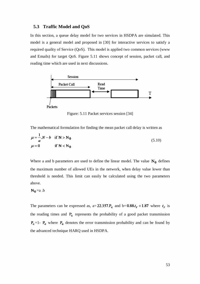
5.3 Traffic Model and QoS

In this section, a queue delay model for two services in HSDPA are simulated. This

model is a general model and proposed in [30] for interactive services to satisfy a

required quality of Service (QoS). This model is applied two common services (www

and Emails) for target QoS. Figure 5.11 shows concept of session, packet call, and

reading time which are used in next discussions.

Figure: 5.11 Packet services session [34]

The mathematical formulation for finding the mean packet call delay is written as

(5.10)

Where a and b parameters are used to define the linear model. The value defines

the maximum number of allowed UEs in the network, when delay value lower than

threshold is needed. This limit can easily be calculated using the two parameters

above.

=a .b

The parameters can be expressed as, a= and b= where is

the reading times and represents the probability of a good packet transmission

=1- where denotes the error transmission probability and can be found by

the advanced technique HARQ used in HSDPA.

53

5.3.1 Results and Discussions In this scenario, the probability of a good packet transmission is set to cP =0.5. The

reading time for Email is set to 20 seconds, and for web browsing is 7 seconds for

target QoS. Figure 5.12 shows resultant model for the mentioned services. The

queuing delay model is a general model and can be applied in realistic transmission

scenarios so as to satisfy a required Quality of Service.

Figure: 5.12 Mean packet call delay for two services

The lines in Figure 5.12 are drawn for the two services to get target QoS. The lines

are considered as thresholds and can be thought of as an excellent QoS. All delay

values smaller than these thresholds are negligible and are considered zero. The

simulations show that the mean delay µ depends on the number of UEs in the

network, the probability of a good packet transmission cP and the Reading Time rt . It

can be observed from the figure that the mean delay becomes a linear finction of N

when the number of UEs present in the network crosses a certain value.

Different statistics of the mean delay are generated. For example, the 95-percentile

values of µµτ 305.0ln. =−= . Besides all, this model is true for all fair scheduling

algorithms [30]. As said earlier, this model is dependent on the probability of a good

54

packet transmission. The model is simulated with different cP values for both of the

services. Figure 5.13 and 5.14 shows the results.

Figure 5.13: Mean packet call delay of Email for different probability values cP

Figure 5.14: Mean packet call delay of web browsing for different probability values

cP

55

5.4 Delays and QoS Classes

In this section Real-Time packet schedulers are simulated and differentiate the desired

QoS based on packet delays. First Modified Largest Weighted First (M-LWDF)

algorithm is simulated and the two classes based on delays are differentiated HSDPA

cell with 20 users are selected. The generation of SNR values, mapping of SNR into

CQI and then to the data rates are all the same as it was in the earlier section. The

scenario is made when the Head of line (HOL) packet delay increases at the base

station, then that user will get priority. The simulation is performed in such way that

the high delay packets are given high priority and is considered as “class 1” users.

When the delays are small, the algorithm behaves as Proportionally Fair. The QoS

parameters are set for both traffic classes. Figure 5.15 shows the simulated result of

this algorithm.

Figure 5.15: Data Rates of Two Classes with M-LDWF

Their corresponding delays for both of the classes are shown in the Figure 5.16.

56

Figure 16: Delay versus number of users

Next the same scenario with the Exponential Rule algorithm are simulated. All the

parameters are the same as for M-LWDF (QoS parameters, delay etc) but this

algorithm introduces exponential term that’s why it is known as Exponential Rule

algorithm. If the exponent term is close to one then this algorithm behaves as

Proportional Fair (PF) algorithm. On the other hand, if one of the queues is having a

larger (weighted) delay than the others by more than order Wa , then the priority is

given to that user (i). The highest priority is given to the “class 1” users. The

simulated result for both of the classes differentiated by QoS parameters is shown in

Figure 5.17 and Figure 5.18.

57

Figure 5.17: Data Rates of two Classes

Figure 5.18: Delay versus Users

It has also been observed that the throughput of EXP-Rule is less than the M-LWDF.

This policy gracefully adopts from a Proportional Fair which balances delays. Figure

5.18 show that this algorithm balances the delays. The standard deviations for both

kinds of the classes are shown in the figures 5.19 and 5.20 below. The standard

deviation of “class 1” is 9.03 while the standard deviation of “class 2” is 10.04.

Figure 5.19 Standard deviation of Class 1 Figure 5.20 Standard deviation of Class 2

Next simulation of SNR, PF, and EXP-Rule algorithms all together is carried out.

Delays are introduced in all of the algorithms and checked the performance of all of

them. It is also known that the SNR and PF algorithms do not account for delays of

packets and can result in poor delay performance. The result in Figure 5.21 shows that

the Exponential Rule balances the delays while SNR and PF algorithms do not

58

account for balances. The standard deviation of SNR, PF, and EXP-Rule is 197, 106

and 8 respectively. The advantage of EXP-Rule is that it balances the delays and

prioritizes the users according to their QoS parameters. But the drawback of this

algorithm is that it reduces the throughput. The comparison between throughputs for

the same amount of number of users in the mentioned algorithms is shown in Figure

5.20 and their corresponding delays is shown in Figure 5.21

Figure: 5.20 Data Rates of the algorithms

Figure: 5.21 Delay Vs number of users

59

Chapter 6

6 Conclusions and Future Work

6.1 Conclusions

QoS is the ability to provide resources and prioritize different applications. As

mentioned before, the 3GPP standard defines four categories of service

(Conversation, streaming, interactive and background) for UMTS. Strategies in traffic

management, priority GBR allowances and bandwidth are important strategies for

traffic differentiation and quality of service (QoS). Providing QoS over HSDPA is

one of the challenging tasks for researchers. The significant results and findings of our

thesis are as follows

• In this thesis various algorithms were implemented with their duties barrier to

provide guarantees of quality, in terms of speed guaranteed (GBR). The emphasis was

to ensure the flow and priority categories of traffic. First the performance of

algorithms were studied alone and then along with the barrier functions. It is

concluded that barrier functions play an important role by means of providing QoS

guarantee in HSDPA, considering channel conditions. Traffic classes were prioritized

on QoS parameters defined for barrier functions. It was found that minimum bit rates

were maintained by barrier functions but the cell throughput decreases with their

barrier functions depending upon QoS parameters. The streaming aware scheduler has

been evaluated by means of simulations in mixed scenarios and it is concluded that

this algorithm protects streaming QoS in high overload conditions. It is therefore

concluded that barrier functions and streaming aware schedulers are the best option

for QoS control. These schedulers are very simple and consider diversity gains as

well.

6.2 Future Work

In this thesis the focus was on different algorithms programming functions barrier to 60

differentiate the different services and deliver quality service. The study was also

developed, using the classic theory of telecommunications traffic loss and delay

models to provide resources to different classes of traffic. Moreover, this argument

can be extended in the future. There are few questions that are proposed for future

work.

The schedulers suggested in the literature depends on SNR values and their CQIs.

The performance of different schedulers was observed in Chapter 5. Different

schedulers can be used at a time to benefit from different algorithms for optimization

point of view. Clusters of a cell can be made and apply different algorithms

according to SNR values. For QoS differentiations, barrier functions or streaming

aware schedulers may be used to control QoS constraints. But the task is left on the

researchers for pros and cons and complexity by using more than one algorithm in a

cell.

61

References [1]. H. Holma and A. Toskala, HSDPA/HSUPA for UMTS, John Wiley and Sons,Ltd, ISBN 978-0-470-018844-2 April, 2006 [2]. “Physical Layer Procedure”, 3GPP Technical Specification 25.214 version 6.4.0, January 2005 [3]. QoS for UMTS Iu Data Bearer Protocols [4]. P. Ameigeiras, “Packet Scheduling and Quality of Service in HSDPA,” PhD Dissertation, Department of Communication Technology, Aalborg University, Denmark, October 2003. [5]. Agilent Technologies,” Concepts of HSDPA: Bringing increased throughput and efficiency to WCDMA”, literature part number 5989-2365ESN, November, 2005. [6]. K. I. Pedersen, P. E. Mogensen, and T E. Kolding,” Overview of QoS Options for HSDPA”, IEEE Communication Magazine, July 2006. [7]. K. I. Pedersen, P. E. Mogensen, and T E. Kolding, “ QoS Consideration for HSDPA and Performance Results for Different Services”, Vehicular Technology Conference, IEEE, September, 2006. [8]. K. I. Pedersen, J. Wigard, F. Frederickson and P. E. Mogensen, “High Speed Downlink Packet Access: WCDMA Evolution”, IEEE Vehicular Technology Society News, February 2003. [9]. E.G. Jung, J. Kim, and Y. Han, “ A New Hybrid Packet Scheduling Algorithm with QoS Provision in HSDPA”, ICACT, February, 2007. [10]. A. Mader, D. Staehle and H. Barth, “A Novel Performance Model for the HSDPA with Adaptive Resource Allocation”, PP 950-961 ITC, 2007. [11]. Usman Shahid, “HSDPA modelling for UMTS”, Master thesis, Department of Communication Optics and Materials, Technical University of Denmark, Denmark, July, 2005. [12]. Husain Samreen, “Delay based Scheduling Algorithm for HSDPA” Master thesis, Department of School of computing, Queen’s University, Kingston, Ontario, Canada, August 2007. [13]. T. E. Kolding, F. Frederickson, P. E. Mogensen, “Performance aspects of WCDMA systems with High Speed Downlink Packet Access”. IEEE Vehicular Technology, 2002. [14]. S. Dixit, Y. Guo and Z. Antoniou,” Resource Management and Quality of Service in Third-Generation Wireless Networks.” IEEE Communication Magazine, February, 2001. [15]. Y.Guo and H. Chaskar,”A Framework for Quality of Service Differentiation on 3G CDMA air interface, Wireless Communications and Networking Conference, IEEE, 2002. [16]. “QoS Concept and Architecture Release 7”, 3GPP Technical Specification 23.107 version 7.1.0, August 2007. [17]. M. Andrews, K. Kumaran, K. Ramanan, A.Stolyer and P: Whiting “Providing Quality of Service over a shared Wireless Link”. IEEE Communication Magazine, February 2001. [18]. G. Aniba and S. Aissa, “ A general traffic and queuing delay model for 3G wireless packet networks, 11th International Conference on Telecommunications, ICT, August,2004 [19]. Sanjay Shakkottai and A.L.Stolyar, “Scheduling Algorithms for a Mixture of Real Time and Non Real Time Data in HDR” Bell Labs, Lucent Technologies Murray Hill, NJ 07974.

62

[20]. Barriac G.and Holtzman, “Introducing Delay Sensitivity into the Proportional Fair Algorithm for CDMA Downlink Scheduling”. Spread Spectrum Techniques and Applications, IEEE 7th International Symposium,2002 [21]. M. Malkowski, A. Kemper, and X.Wang “Performance of Scheduling Algorithms for HSDPA”. Spread Spectrum Techniques and Applications, IEEE,2002 [22]. D. Tse, “Forward Link Multi-user Diversity through Rate adaptation and scheduling” .IEEE JSAC. [23]. Y. Min and, D. Ku. Kim, “Packet Scheduling Algorithms for Throughput Fairness and Coverage Enhancement in TTD-OFDMA Downlink Network” .IEICE TRANS COMMUN, November, 2005. [24]. Patrick A.Hosein,” QoS control for WCDMA High Speed Packet Data,” IEEE, Mobile and Wireless Communication Network, 4th International Workshop on volume, 2002, pp 169-173. [25]. M. Lundevall, B.Olin, J. Olesson, N. Wiberg and S. Wanstedt, “Streaming Applications over HSDPA in Mixed Service Scenarios” Vehicular Technology Conference, 2004 IEEE [26]. T. E. Kolding, “Link and system performance aspects of proportional fair scheduling in WCDMA/HSDPA”, IEEE VTC 2003 fall, USA, October 2003. [27]. C. Necker, “A comparisons of scheduling mechanisms for service class differentiations in HSDPA networks”, AEU international journal of Electronics and Communications, October 2006. [28]. 3gpp Technical Specification Group Radio Access Network HSDPA overall Description Stage 2 (Release 6) [29]. Jonas Eriksson, “Providing QoS in Streaming for Evolved 3G Networks” Linkoping University , Sweden, 2004. [30]. G. Aniba and Sonia Aissa, “A Queuing Delay Model for Dimensioning Interactive Service Traffic in HSDPA Networks”, International Conference on Wireless Networks, Communications and Mobile Computing, 2005. [31].http://mobilesociety.typepad.com/mobile_life/2007/03/a_real_life_com.html [32]. epubl.luth.se/1402-1617/2007/246/LTU-EX-07246-SE.pdf [33]. E. Iliakis and G. Kardaras,” Resource Allocation in Next Generation Internet,” Master thesis, Department off Communication Optics and Materials, Technical University of Denmark, Denmark, 2007 [34]. Sylvain Ranvier,” Path Loss Models,” Helsinki University of Technology (HUT), Finland, November, 2004, [35]. Rob Dalgeish,” HSDPA Applications and System Performance”, IEEE VTC, Orlando October, 2003,

63