Chapter 4

The door beckoned, so he pushed through it. Even the street was better lit. He didn’t knowhow, he just knew—the patron seated at the corner table was his man. Spectacles, unkept hair,old sweater, one bottle, one glass. Elbows on the bar and foot on the rail, he strained for calmnessuntil the barkeep finally appeared. A meek “bourbon, rocks,” left his lips, then he shuffled a billhe thought was a five onto the bar, pocketed the change, tugged on the drink, and let his feet movehim to the corner table. “I wanna talk to you....” The stranger slowly greeted him with his eyes,as if he was expected, and replied “What about, son?” Resisting the urge to look away, the wordsjust fell “: : :those Rutherford rays: : :”

Scattering in One DimensionThe free state addressed in the last chapter is the simplest problem because the potential

is chosen to be zero. The next simplest problems are those where the potentials are piecewiseconstant. A potential that is piecewise constant is discontinuous at one or more points. Thepotential is chosen to be zero in one region and is of non-zero value in other regions without atransition region. A discontinuity in a potential is not completely realistic though these problemsdo model some realistic systems well. Transistors, semiconductors, and alpha decay (Rutherfordrays) are examples for which an abrupt change in potential is a key feature. Though they arenot perfect models, piecewise constant potentials do contain some realistic physics and serve toillustrate features of potentials that are very steep.

The primary reason to address these problems is that a discontinuous change in potentialis much more mathematically tractable than a continuous change. These problems are usuallyaddressed using the position space, time-independent form of the Schrodinger equation. Thestrategy is to divide space into regions at the locations where the potential changes and thenattain a solution for each region. The points at which the potential changes are boundaries.The wavefunction and its first derivative must be the same on both sides of the boundaries.Equating the wavefunctions and their first derivatives at the boundaries provides a system ofequations that yield descriptive information. Also, solving problems in one dimension is usuallymathematically attractive and can be realistic. One dimensional situations are often a precursorto multi-dimensional situations.

There is some key quantum mechanical behavior in these problems. You should absorb theidea that a particle has a non-zero probability to appear on the other side of a potential barrierthat it does not classically have the energy to surmount. This is known as barrier penetration ortunneling. Also, a particle has a non-zero probability to be reflected at any boundary regardlessof energy. For instance, a particle possessing enough energy to surmount a potential barrier canstill be reflected. You should learn the terms reflection and transmission coefficients.

A particle is in either a free state (chapter 3), a bound state (chapter 5, 6, and parts ofothers), or a scattering state. The bound state is described by a potential that holds a particlefor a non-zero time period. The scattering state can be described as an interaction of a free particlewith a potential that results in a free particle. If a free particle interacts with the potential anddoes not become bound, the particle is in a scattering state. The hydrogen atom may be ionized.The electron can escape and enter a free state, but it cannot escape without the influence of anexternal photon. Scattering concerns the situation where there is no external influence.

Finally, you should also appreciate the presence of the postulates of quantum mechanics.

201

Though the position space, time-independent Schrodinger equation dominates the discussion, re-member that it is simply a convenient form of the sixth postulate.

1. Find the reflection and transmission coefficients for a particle of energy E > V0 incident fromthe left on the vertical step potential

V (x) ={

0 if x < 0 region 1 ,V0 if x > 0 region 2 .

Notice that region 2 extends to infinity. This is an approximation to a potential that is very steepbut not perfectly vertical, and of significant though not of infinite width. If the step is not vertical,it is difficult to match boundary conditions, and if the step is not of infinite extent, “tunneling”(see problem 3) is possible.

Particles that are incident from the left will either be reflected or transmitted. The reflectioncoefficient, denoted R , is classically defined as the ratio of intensity reflected to intensity inci-dent. The classical transmission coefficient, denoted T , is the ratio of intensity transmitted tointensity incident. Quantum mechanically, intensity is analogous to probability density. Quantummechanical transmission and reflection coefficients are based on probability density flux (problem2). The reflection and transmission coefficients must sum to 1 in either classical or quantummechanical regimes.

The two physical boundary conditions applicable to this and many other boundary valueproblems are the wave function and its first derivative are continuous.

A general solution to the Schrodinger equation for a particle approaching from the left is

ˆ1 (x) = Aeik1x + B e−ik1x; x < 0 ;

ˆ2 (x) = C eik2x; x > 0 ;

where the subscripts on the wavefunctions and wave numbers indicate regions 1 or 2, and

k1 =

√2mE

h̄and k2 =

√2m (E − V0)

h̄:

The ki are real because E > V0 . In region 1, the term Aeik1x is the incident wave and B e−ik1x

describes the reflected wave. C eik2x models the transmitted wave in region 2. A term likeD e−ik2x , modeling a particle moving to the left in region 2, is not physically meaningful for aparticle given to be incident from the left. Equivalently, D = 0 for the same reason. Applying theboundary condition that the wavefunction is continuous,

ˆ1 (0) = ˆ2 (0) ⇒ Ae0 + B e0 = C e0 ⇒ A + B = C :

The derivative of the wavefunction is

ˆ′1 (x) = Aik1 eik1x − B ik1 e−ik1x; x < 0 ;

202

ˆ′2 (x) = C ik2 eik2x; x > 0 ;

so continuity of the first derivative means

ˆ′1 (0) = ˆ′

2 (0) ⇒ Aik1 eik1(0) − B ik1 e−ik1(0) = C ik2 eik2(0) ⇒ k1(A − B

)= k2 C :

We now have two equations in the three unknowns A; B, and C. Eliminating C ,

k1(A − B

)= k2

(A + B

)⇒

(k1 − k2

)A =

(k1 + k2

)B ⇒ B =

(k1 − k2

k1 + k2

)A:

From this relation we can calculate the reflection coefficient. The incident probability density is

∣∣ A eik1x∣∣2 =

(Aeik1x

)∗(A eik1x

)=

(A∗e−ik1x

)(Aeik1x

)= A∗A e0 =

∣∣ A∣∣2;

or the intensity of the incident wave is the square of the norm of the coefficient of the incidentwave. Similarly, the intensity of the reflected wave is

∣∣ B∣∣2, and the intensity of the transmitted

wave is∣∣ C

∣∣2. In this specific problem the reflection coefficient is

R =

∣∣ B∣∣2

∣∣ A∣∣2 =

(k1 − k2

k1 + k2

)2 ∣∣ A∣∣2

/∣∣ A∣∣2 =

(k1 − k2

k1 + k2

)2

and

R + T = 1 ⇒ T = 1 − R = 1 −(

k1 − k2

k1 + k2

)2

=(

k1 + k2

k1 + k2

)2

−(

k1 − k2

k1 + k2

)2

=4k1k2(

k1 + k2)2 :

Postscript: Classically, R = 0 and T = 1 if E > V0 . Figure 4–2 illustrates the quantum

mechanical analogy. What does it mean that R > 0 when E > V0 ? For a single particle,it means that a portion of the wavefunction is transmitted and a portion of the wavefunction isreflected. Postulate 4 says that you can calculate the probabilities for finding the particle in region1 or 2 from the probability amplitudes, but can do no better. If you look, you will find the particlein either region 1 or region 2 per postulate 3, and the measurement will leave the state vector inthe eigenstate corresponding to the location that you measured per postulate 5. The probabilityof finding the particle in the other region is then zero.

Notice that the particle will have longer wavelength and thus less momentum in region 2 sincethe energy relative to the “floor” of the potential is less in region 2 than region 1.

The classical trajectory of a particle is continuous and a change in trajectory (the first deriva-tive) will be continuous. Quantum mechanically, refined arguments are necessary. The validity ofthe two boundary conditions can be demonstrated for a Gaussian wavefunction. The issue becomesthat a wave packet that is quantized in wave number will scatter from a potential with preciselythe same reflection and transmission coefficients as a Gaussian wavefunction. This can be donefor a wave packet quantized in wave number that is still smooth compared to the scale of the

203

potential variations. This is a non-trivial calculation that is beyond our scope. The point is thatthe boundary conditions of continuity of the wavefunction and its first derivative are also justifiedquantum mechanically.

2. (a) Calculate the amplitude C of the transmitted portion of the wavefunction in terms of thecoefficient A for the vertical step potential of problem 1.

(b) Show that the ratio | C | 2= |A | 2 is 6= T from problem 1.

(c) Rectify the discrepancy between part (b) and the result of problem 1.

Parts (a) and (b) are intended to demonstrate a counter-intuitive fact that is explained in part(c). Use intermediate results from problem 1 to solve for C in terms of A . Form the ratio| C | 2= |A | 2 which is not the same as T from problem 1. Part (c) requires that you know thatflux is velocity times intensity. Since the particle has a different height above the floor of thepotential in regions 1 and 2, it has not only a different wavenumber but a different velocity. Thesevelocities are related to the de Broglie relation. The ratio v2 |C | 2=v1 | A | 2 is the transmissioncoefficient found in problem 1.

(a) Using intermediate results from problem 1, the amplitude of the transmitted portion is

C = A + B = A +(

k1 − k2

k1 + k2

)A =

(k1 + k2

k1 + k2

)A +

(k1 − k2

k1 + k2

)A =

(2k1

k1 + k2

)A :

(b) The ratio of the squares of the magnitudes is not the transmission coefficient of problem 1,

∣∣ C∣∣2

∣∣ A∣∣2 =

(2k1

k1 + k2

)2

|A | 2/

| A | 2 =4k2

1(k1 + k2

)2 6= 4k1k2(k1 + k2

)2 :

(c) These differ because the energy, and thus the velocity, of the wave changes as the particlecrosses the step. Flux is intensity times velocity. Probability density flux, probability density

times velocity, is appropriate for a quantum mechanical description. Since vi =pi

m=

h̄ki

m;

T =v2

∣∣ C∣∣2

v1∣∣ A

∣∣2 =h̄k2=m

∣∣ C∣∣2

h̄k1=m∣∣A

∣∣2 =k2

∣∣C∣∣2

k1∣∣ A

∣∣2 = k2

(2k1

k1 + k2

)2

|A | 2

/k1 |A | 2 =

4k1k2(k1 + k2

)2 ;

consistent with the problem 1.

Postscript: A reflected wave is the same height above the floor of the potential as the incidentwave so the reflected wave has the same energy, velocity, and wave number as the incident wave.The velocities cancel in region 1 so are not considered in calculating the reflection coefficient, i.e.,

R =v1

∣∣B∣∣2

v1∣∣ A

∣∣2 =

∣∣ B∣∣2

∣∣ A∣∣2 :

204

3. Determine the transmission coefficient for a particle with E < V0 incident from the left on therectangular barrier

V (x) ={

V0 for −a < x < a ,0 for | x | > a .

If the energy of the particle is less than the height of the step, and the “ potential plateau” is offinite length, the particle incident from the left can appear on the right side of a barrier. This isa non–classical phenomena known as barrier penetration or tunneling. Classically, if a ballis rolled up a ramp of height h with kinetic energy K , the ball will roll back down the ramp ifK < mgh . A quantum mechanical ball has a non–zero probability that the ball would appear onthe other side of the ramp in the case K < mgh .

This is a boundary value problem with three regions because there are two boundaries. Thestrategy is to require continuity of the wavefunction and its first derivative at all boundaries andsolve for the transmission coefficients in terms of the ratios of the squares of the appropriatewavefunction coefficients.

(a) Divide “all space” into three regions at the boundaries of the potential ±a . The wavefunctionsconsist of a linear combination of waves in both directions in each of the three regions:

ˆ1 (x) = Aeikx + B e−ikx for x < −a ;

ˆ2 (x) = C e•x + D e−•x for − a < x < a ;

ˆ3 (x) = F eikx + G e−ikx for x > a ;

where k =√

2mE =h̄ and • =√

2m (V0 − E) =h̄ . Notice that • is defined so that it is real forE < V0 . This is a technique that leads to minor simplifications. Conclude that G = 0 because itis the coefficient of an oppositely directed incident wave, and therefore, is not physical.

(b) Apply the boundary condition that the wavefunction must be continuous at the boundaries.This yields two equations. Differentiate the wavefunction and then apply the boundary conditionthat the first derivative of the wavefunction must be continuous at boundaries. This yields twomore equations. Eliminating B from the two equations for the left boundary, you should find

2Ae−ika =(

1 −i•

k

)C e−•a +

(1 +

i•

k

)D e•x:

Using the two equations at the right boundary to solve for two of the unknown coefficients in termsof the coefficient F , you should find

C e•a =12

(1 +

ik

•

)F eika and D e−•a =

12

(1 −

ik

•

)F eika:

(c) Use the last two equations to eliminate the coefficients C and D from the first equation so

Ae−ika = F eika

[cosh (2•a) +

i(•2 − k2)2k•

sinh (2•a)]

:

205

Remember that sinh (x) =ex − e−x

2and cosh (x) =

ex + e−x

2:

(d) A reflected and transmitted particle will be the same height above the floor of the definedpotential so the transmission coefficient is the ratio of probability density of that portion of thewavefunction which “goes through” the barrier, represented by | F | 2 , to the incident probabilitydensity, represented by | A | 2 . The reciprocal of this ratio, | A | 2= | F | 2 , is

T −1 = 1 +V 2

0

4E (V0 − E)sinh2

(2a

h̄

√2m (V0 − E )

);

which is a more pleasing and compact expression than T that still indicates T 6= 0 when E < V0 .

(a) For the region x > a ; ˆ (x) = F eikx + G e−ikx, and G = 0 because it is the coefficient of anoppositely directed incident wave that cannot be physical. So the wave function is

ˆ (x) =

Aeikx + B e−ikx; for x < −a ,C e•x + D e−•x; for −a < x < a ,F eikx; for x > a ,

where k =√

2mE = h̄ and • =√

2m (V0 − E) = h̄ .

(b) There are three regions so there are two boundaries. Continuity at the boundaries requires

Ae−ika + B eika = C e−•a + D e•a; x = −a ; and (1)

C e•a + D e−•a = F eika; x = a ; (2)

so there are two equations in five unknowns. The derivative of ˆ (x) is

ˆ′ (x) =

Aik eikx − B ik e−ikx; for x < −a ,C •e•x − D • e−•x; for −a < x < a ,F ik eikx; for x > a .

Applying the boundary condition of continuity of the first derivative at x = −a ,

Aik e−ika − B ik eika = C •e−•a − D • e•a; and at x = a ; (3)

C •e•a − D •e−•a = F ik eika: (4)

There are now four equations in five unknowns. Multiplying equation (1) by ik ,

B ik eika = C ik e−•a + D ik e•a − Aik e−ika:

Substituting this into equation (3) for B ik eika,

Aik e−ika − C ik e−•a − D ik e•a + Aik e−ika = C •e−•a − D • e•a

⇒ 2Aik e−ika = C ik e−•a + C • e−•a + D ik e•a − D •e•a

= C (ik + •) e−•a + D (ik − •) e•a

206

⇒ 2Ae−ika =(

1 −i•

k

)C e−•a +

(1 +

i•

k

)D e•a: (5)

Multiplying equation (2) by • and solving for the term with the coefficient D,

D •e−•a = F • eika − C • e•a

Substituting the right side into equation (4) for D •e−•a,

C •e•a − F • eika + C •e•a = F ik eika

⇒ 2C •e•a = F •eika + F ik eika = F (• + ik) eika

⇒ C e•a =12

(1 +

ik

•

)F eika: (6)

Multiplying equation (2) by • and solving for the term with the coefficient C ,

C •e•a = F •eika − D • e−•a

Substituting the right side into equation (4) for C •e•a,

F •eika − D • e−•a − D •e−•a = F ik eika

−2D • e−•a = −F• eika + F ik eika = F (−• + ik) eika

⇒ D e−•a =12

(1 − ik

•

)F eika: (7)

(c) The signs on the exponentials in equations (6) and (7) are opposite those in equation (5), so

C e•a =12

(1 +

ik

•

)Feika ⇒ C e−•a =

12

(1 +

ik

•

)F eikae−2•a;

D e−•a =12

(1 −

ik

•

)F eika ⇒ D e•a =

12

(1 −

ik

•

)F eikae2•a;

and now the signs of the exponentials are consistent. Substituting these into equation (5),

⇒ 2Ae−ika =(

1 −i•

k

)12

(1 +

ik

•

)F eikae−2•a +

(1 +

i•

k

)12

(1 −

ik

•

)F eikae2•a

=F eika

2

(1 − i•

k+

ik

•+

•k

•k

)e−2•a +

F eika

2

(1 +

i•

k− ik

•+

•k

•k

)e2•a

=F eika

2

(2e−2•a − i•

ke−2•a +

ik

•e−2•a + 2e2•a +

i•

ke2•a − ik

•e2•a

)

=F eika

2

[2(e−2•a + e2•a

)−

i•2

k•e−2•a +

ik2

k•e−2•a +

i•2

k•e2•a −

ik2

k•e2•a

]

=F eika

2

[2(e−2•a + e2•a

)+

i•2

k•

(e2•a − e−2•a

)−

ik2

k•

(e2•a − e−2•a

)]

= F eika

[2(

e2•a + e−2•a

2

)+

i(•2 − k2)k•

(e2•a − e−2•a

2

)]

207

⇒ Ae−ika = F eika

[cosh (2•a) +

i(•2 − k2)2k•

sinh (2•a)]

:

(d) The transmission coefficient is the ratio of intensity transmitted, represented by |F | 2, tothe intensity incident, represented by | A | 2. It is conventional to calculate the reciprocal of thisratio to arrive at a compact expression. Both sides are in the polar form of complex numbers, i.e.,magnitude and phase. The last result can be arranged as the ratio

∣∣∣∣Ae−ika

F eika

∣∣∣∣ =∣∣∣∣[

cosh (2•a) +i(•2 − k2)

2k•sinh (2•a)

] ∣∣∣∣ :

Now∣∣∣∣A e−ika

F eika

∣∣∣∣ =[

Ae−ika

F eika

A∗eika

F ∗e−ika

]1=2

=[

AA∗

F F ∗

]1=2

=

[AA∗ ]1=2

[F F ∗

]1=2=

∣∣ A∣∣

∣∣ F∣∣

⇒| A | 2

|F | 2 =∣∣∣∣[

cosh (2•a) +i(•2 − k2)

2k•sinh (2•a)

] ∣∣∣∣2

= cosh2(2•a)+(

(•2 − k2)2k•

)2

sinh2(2•a);

where we have used the fact the product of complex conjugates is sum of the squares of the realpart and the coefficient of the imaginary part. Recalling that cosh2 (x) = 1 + sinh2 (x ) ,

|A | 2

|F | 2 = 1 + sinh2 (2•a) +(

•4 − 2k2•2 + k4

4k2•2

)sinh2 (2•a)

= 1 +(

1 +•4 − 2k2•2 + k4

4k2•2

)sinh2 (2•a)

= 1 +(

4k2•2 + •4 − 2k2•2 + k4

4k2•2

)sinh2 (2•a)

= 1 +(

•4 + 2k2•2 + k4

4k2•2

)sinh2 (2•a)

= 1 +

(•2 + k2

)2

4k2•2 sinh2 (2•a) :

Substituting k =√

2mE = h̄ and • =√

2m (V0 − E) = h̄ ,

|A | 2

| F | 2 = 1 +

(2m

h̄2 (V0 − E) +2m

h̄2 E

)2

4(

2m

h̄2 E

) (2m

h̄2 (V0 − E)) sinh2

(2a

h̄

√2m (V0 − E )

)

= 1 +

4m2

h̄4 (V0 − E + E)2

4m2

h̄4 4E (V0 − E)sinh2

(2a

h̄

√2m (V0 − E)

)

⇒ |A | 2

|F | 2 = T −1 = 1 +V 2

0

4E (V0 − E)sinh2

(2a

h̄

√2m (V0 − E )

):

4. Determine the transmission coefficient for a particle with E = V0 incident from the left on therectangular barrier defined in the last problem.

208

The intent of this problem is to further develop your skills applying boundary conditions. Requirecontinuity of the wavefunction and its first derivative at all boundaries.

The first step, which is non-trivial, is to write a proper wavefunction. Similar to problem 3,the wavefunction in the three regions can be written as

ˆ1 (x) = Aeikx + B e−ikx for x < −a ;

ˆ2 (x) = C + D x for − a < x < a ;

ˆ3 (x) = F eikx for x > a :

The wave number is the same in regions 1 and 3 because particle energy is the same height abovethe “floor,” and is zero in region 2 for either possible definition because E = V0 . Follow parts(b) through (d) of problem 3 to get the reciprocal of the transmission coefficient,

T −1 = 1 +2mE

h̄2 a2 :

When E = V0 , the wavenumber in the region −a < x < a is k =√

2m (V0 − E) = h̄ = 0 , so

the wavefunction can be written ˆ (x) =

Aeikx + Be−ikx; for x < −a ,C + Dx ; for −a < x < a ,Feikx; for x > a .

Continuity of the wavefunction at x = −a means

Ae−ika + B eika = C − D a ; (1)and at x = a ; C + D a = F eika: (2)

Continuity of the derivative of the wavefunction at x = −a means

A ik e−ika − B ik eika = D ; (3)and at x = a ; D = F ik eika: (4)

Multiplying equation (1) by ik and solving for the term with the coefficient B yields

B ik eika = ik C − ik D a − Aik e−ika:

Substituting this into equation (3) eliminates the unknown coefficient B ,

Aik e−ika − ik C + ik D a + Aik e−ika = D

⇒ 2Aik e−ika = ik C + D (1 − ika) : (5)

Equation (2) can be written C = F eika − D a ; and substituting this into equation (5),

2Aik e−ika = ik (Feika − D a) + D (1 − ika)

= ik Feika − ik D a + D (1 − ika)

= ik F eika + D (1 − 2ika ) :

209

Substituting equation (4) into the last equation eliminates the unknown coefficient D ,

2Aik e−ika = ik F eika + F ik eika (1 − 2ika)

⇒ 2Ae−ika = F eika + F eika (1 − 2ika)

⇒ 2Ae−ika = F eika (2 − 2ika)

⇒ Ae−ika = F eika (1 − ika)

⇒ Ae−ika

F eika= 1 − ika

and∣∣∣∣Ae−ika

F eika

∣∣∣∣ =∣∣∣∣A

F

∣∣∣∣ =|A || F |

as previously shown,

⇒ |A |2

| F |2=

∣∣ 1 − ika∣∣2 = 1 + k2a2:

Substituting k =√

2mE = h̄ ;|A |2

| F |2= T −1 = 1 +

2mE

h̄2 a2 for E = V0 :

5. Show in the limit E → V0 from below, that the results of problems 3 and 4 are equivalent.

The intent of this problem is to demonstrate self-consistency by examining a limiting case. It isa technique that is difficult to teach and important to learn. Start with the result of problem 3.Expand sinh (x) and ignore the higher order terms so that sinh (x) ≈ x since E ≈ V0 . Of course,in the limit E → V0 the results of problem 3 and 4 must be the same.

Start with the reciprocal of the transmission coefficient from problem 3. Ignoring higher orderterms as negligible in the series expansion of sinh (x) ⇒ sinh (x) ≈ x ,

T −1 = 1 +V 2

0

4E (V0 − E)

(2a

h̄

√2m (V0 − E)

)2

= 1 +V 2

0

4E (V0 − E)

(4a2

h̄2 2m (V0 − E))

= 1 +V 2

0

E

(a2

h̄2 2m

)

= 1 +2mV 2

0

h̄2Ea2 :

Remembering that E ≈ V0 ; T −1 ≈ 1 +2mE

h̄2 a2 :

6. (a) A particle of energy E > V0 is incident on a rectangular barrier of width 2a . Solve forthe value of the transmission coefficient and locate the positions of the maxima and minima interms of wave number. Plot transmission coefficient versus barrier width for a particle of constantenergy and variable barrier width.

210

(b) Locate the positions of the maxima in terms of particle energy. Plot transmission coefficientversus particle energy where E > V0 and barrier width is fixed.

This problem introduces a phenomenon known as resonance scattering. At certain values ofparticle wave number (energy), there is 100% transmission and no reflection. Part (a) shouldillustrate resonance scattering for an incident particle of fixed energy and a barrier width that isvaried. Part (b) illustrates the same phenomenon where particle energy is varied and barrier widthis fixed. Start with an intermediate result from problem 10,

1T

= 1 +14

(k21 − k2

2

k1k2

)2

sin2 (2k2a ) :

Solve for T instead of its reciprocal. The maxima occur where the sine term is zero at barrierwidths of 2a = n…=k2 . The minima occur where the sine term is one, where the transmission

coefficient has the value T =(

2k1k2

k21 + k2

2

)2

: Part (b) is likely easiest if started with

1T

= 1 +V 2

0

4E (E − V0)sin2

(2a

h̄

√2m (E − V0)

);

the result of problem 10 in terms of energy. Again, solve for T instead of its reciprocal. This plotis more difficult because the independent variable E appears in five places including the squareroot of the sine squared term. The important part of this graph is the shape. If you do not haveaccess to a commercial graphing package, try to imagine what the graph should look like, and skipto the solution. You should find the maxima at

E =…2h̄2

8ma2 n2 + V0 :

This result is closely related to the infinite square well that is encountered in the next chapter.

(a)1T

= 1 +14

(k21 − k2

2

k1k2

)2

sin2 (2k2a) =4k2

1k22

4k21k

22

+k41 − 2k2

1k22 + k4

2

4k21k

22

sin2 (2k2a)

=4k2

1k22 +

(k41 − 2k2

1k22 + k4

2

)sin2 (2k2a)

4k21k

22

⇒ T =4k2

1k22

4k21k

22 +

(k41 − 2k2

1k22 + k4

2

)sin2 (2k2a)

:

Maxima of T = 1 occur where sin2 (2k2a) = 0 , i.e., where 2k2a = n… ⇒ 2a =n…

k2are

the barrier widths at which maxima occur, noting that the width of the barrier is given to be 2a .The minima occur where the sine squared term is one, so minima occur at

T =4k2

1k22

4k21k

22 +

(k41 − 2k2

1k22 + k4

2

)· 1

=4k2

1k22

k41 + 2k2

1k22 + k4

2⇒ T =

(2k1k2

k21 + k2

2

)2

at minima.

211

(b) In terms of particle energy,

1T

= 1 +V 2

0

4E (E − V0)sin2

(2a

h̄

√2m (E − V0)

)

=4E (E − V0) + V 2

0 sin2(

2a

h̄

√2m (E − V0)

)

4E (E − V0)

⇒ T =4E (E − V0)

4E (E − V0) + V 20 sin2

(2a

h̄

√2m (E − V0)

) :

The maxima occur where the sine squared term is zero, so

2a

h̄

√2m (E − V0) = n… ⇒

√2m (E − V0) =

n…h̄

2a

⇒ 2m (E − V0) =…2h̄2

4a2 n2 ⇒ E − V0 =…2h̄2

8ma2 n2

⇒ E =…2h̄2

8ma2 n2 + V0

which are energies that are closely related to theeigenenergies of a particle in an infinite square well.

Postscript: Resonance scattering is the circumstance where 100% transmission occurs.

7. (a) Show in position space that

∆(ˆ′ (x)

)=

2m

h̄2 lim†→0

∫ †

−†

V (x)ˆ (x) dx

is the general value of the discontinuity in the first derivative for an infinite potential.

(b) Calculate the value of the discontinuity in the first derivative for a particle interacting withthe potential well V (x) = −fi – (x) .

Use the conditions that ˆ and ˆ′ are continuous at any boundary of a finite potential. Theremust, however, be a discontinuity in the first derivative at all infinite boundaries. If the value of thediscontinuity can be calculated, the boundary condition for the first derivative is again useful. Themethod of calculating the value of the discontinuity is to put the potential into the Schrodingerequation, integrate around the infinite boundary, and let the limits approach zero from both sides.

For a general potential V (x) , the Schrodinger equation in position space is

−h̄2

2m

d2 ˆ (x)dx2 + V (x)ˆ (x) = E ˆ (x) :

212

If we integrate around the point which is the discontinuity, this is

−h̄2

2m

∫ †

−†

d2 ˆ (x)dx2 dx +

∫ †

−†

V (x)ˆ (x) dx = E

∫ †

−†

ˆ (x) dx;

which assumes that the infinite boundary is at x = 0 . The quantity † is infinitesimal. If we let† → 0, the right side of the equation is zero. The integral of a finite quantity, ˆ (x) , over anarbitrarily small interval is zero. The term with the potential does not vanish because the integralof an infinite quantity, the potential, can be non-zero even for an arbitrarily small interval. So,

lim†→0

∫ †

−†

d2 ˆ (x)dx2 dx =

2m

h̄2 lim†→0

∫ †

−†

V (x)ˆ (x) dx

⇒dˆ (x)

dx

∣∣∣†→0

−dˆ (x)

dx

∣∣∣−†→0

=2m

h̄2 lim†→0

∫ †

−†

V (x)ˆ (x) dx

⇒ ∆(ˆ′ (x)

)=

2m

h̄2 lim†→0

∫ †

−†

V (x) ˆ (x) dx (1)

is the general value of the discontinuity in the first derivative.

(b) A delta function potential is infinite, so employing equation (1),

∆(ˆ′ (x)

)∣∣∣x=0

=2m

h̄2 lim†→0

∫ †

−†

(− fi – (x)

)ˆ (x) dx = −

2m

h̄2 fi ˆ (0) ;

because regardless of how closely † approaches zero, −† < 0 < † meaning that zero remains withinthe limits of integration. Since the value of the delta function that makes its argument zero iswithin the limits of integration, the integral is the wavefunction evaluated at the point that makesthe argument of the delta function zero.

Postscript: An infinite potential models a perfectly rigid and perfectly impenetrable wall. Thewavefunction must be zero at an infinite potential barrier and in the region of infinite potentialbecause the term V ˆ in the Schrodinger equation would be infinite otherwise. There is a non-smooth “corner” in the wavefunction as it goes to zero at any position other than ±∞ , thus thereis a discontinuity in the first derivative of the wavefunction. This physically unrealistic model isuseful to understanding concepts, is mathematically tractable, and is a first approximation to anabrupt and large potential.

8. Calculate the reflection and transmission coefficients for a particle incident on the potential

V (x) = −fi – (x) :

This problem is intended to demonstrate how a potential that includesa delta function is treated specifically, and how to treat a discontinu-ity in general. First, write the wavefunction for two regions becausethe delta function is of “zero” width. The wavenumber is the same inregions 1 and 2 because the particle energy is the same height abovethe potential “floor” in both regions. A ˆ (0) is required. Use eitherˆ1 (0) or ˆ2 (0) , because the condition of continuity of the wavefunc-tion at the boundary ensures that they are the same. We use ˆ2 (0)because it has one fewer terms than ˆ1 (0) . Classically, the reflectioncoefficient must be zero. The quantum mechanical result is non-zero.

213

The solution to the Schrodinger equation in position space is

ˆ1 (x) = A eikx + B e−ikx; x < 0 ; ˆ2 (x) = C eikx; x > 0 ;

where the infinite potential well is at x = 0 . Continuity of the wave function means

A eik(0) + B e−ik(0) = C eik(0) ⇒ A + B = C :

The first derivatives in regions 1 and 2 are

ˆ′1 (x) = ik A eikx − ik B e−ikx; ˆ′

2 (x) = ik C eikx:

We calculated the general value of the discontinuity of the first derivative in problem 7. This isthe difference of the first derivatives in regions 1 and 2, meaning

ˆ′1 (0) − ˆ′

2 (0) = −2m

h̄2 fi ˆ (0)

⇒ ik A eik(0) − ik B e−ik(0) − ik C eik(0) = −2m

h̄2 fiˆ (0) :

Using ˆ2 (0) = C ,

ik A − ik B − ik C = −2m

h̄2 fiC

⇒ ik A − ik B = C

(ik −

2m

h̄2 fi

);

and we use the continuity condition, A + B = C , to eliminate C , so

ik A − ik B =(A + B

)(ik −

2m

h̄2 fi

)

⇒ ik A − ik B = A

(ik −

2m

h̄2 fi

)+ B

(ik −

2m

h̄2 fi

)

⇒ A

(ik/

− ik/

+2mh̄2 fi

)= B

(ik + ik −

2mh̄2 fi

)

⇒ A

(2mh̄2 fi

)= B

(2ik − 2m

h̄2 fi

)

⇒ B = A

[(2m

h̄2 fi

) / (2ik − 2m

h̄2 fi

)]=

mfiA

ikh̄2 − mfi:

The reflection coefficient is

R =

∣∣ B∣∣2

∣∣ A∣∣2 =

(mfiA∗

−ikh̄2 − mfi

) (mfiA

ikh̄2 − mfi

)1

| A | 2 =m2fi2

k2h̄4 + m2fi2=

11 + k2h̄4/m2fi2

:

The transmission coefficient is

T = 1 − R = 1 −m2fi2

k2h̄4 + m2fi2=

k2h̄4 + m2fi2 − m2fi2

k2h̄4 + m2fi2=

k2h̄4

k2h̄4 + m2fi2=

11 + m2fi2

/k2h̄4 :

214

Postscript: Any curve that has a sharp corner has a discontinuity in it’s next order derivative.Delta functions and theta functions can be useful in describing discontinuities. Techniques seenin problems 7 and 8 are useful in a number of areas, the use of delta functions in particular isbecoming increasingly popular, and you will see these techniques in future chapters.

Practice Problems

9. For a particle that encounters a vertical step potential of height V0 , calculate the reflection andtransmission coefficients for the particle energies (a) E = 2V0 , (b) E = 3V0=2 ,(c) E = 1:1V0 , and (d) E = V0 . (e) Explain the result of part (d).

This problem is intended primarily to reinforce the quantum mechanical effect that reflection occursat a step even when E > V0 . It should further familiarize you with reflection and transmissioncoefficients. The boundary value problem for a vertical step potential is solved in problem 1,resulting in the general forms of the reflection and transmission coefficients

R =(

k1 − k2

k1 + k2

)2

and T = 1 − R =4 k1 k2

(k1 + k2)2:

Express the energies of parts (a) through (d) in terms of the wavenumbers to attain the reflectionand transmission coefficients using these equations. You should find an increasing amount ofreflection as the energy of the particle gets closer to the energy of the potential barrier, until atE = V0 , the transmission coefficient is zero. The reason for this is there are artificialities builtinto the model to make it more mathematically tractable. Reread the comments on tunneling toidentify the particular artificiality which founds the 100% reflection of part (d) to answer part (e).

10. Determine the transmission coefficient for a particle with E > V0 incident from the left onthe rectangular barrier defined in problem 3.

Reflection from a potential barrier of energy less than that of the incident particle is another solelyquantum mechanical phenomenon. Start with the wavefunction

ˆ (x) =

Aeik1x + B e−ik1x; for x < −a ,C eik2x + D e−ik2x; for −a < x < a ,F eik1x; for x > a .

Require continuity of the wavefunction and its first derivative at all boundaries. Follow the proce-dures of problem 2. Define k1 =

√2mE = h̄ and k2 =

√2m (E − V0) = h̄ , to find

T −1 = 1 +V 2

0

4E (E − V0)sin2

(2a

h̄

√2m (E − V0)

):

215

11. Show in the limit E → V0 from above, that the result of problems 4 and 10 are equivalent.

This problem has the same intent as problem 5. Start with the result of problem 10. Expandsin (x) and ignore the higher order terms so that sin (x) ≈ x since E ≈ V0 . You must find thatin the limit E → V0 the results of problems 10 and 4 are the same.

12. A particle of E > 0 approaches the negative vertical step potential

V (x) ={

0; for x < 0,−V0 for x > 0.

What are the reflection and transmission coefficients if E = V0=3 , and E = V0=8 ?

This problem parallels the discussion of the vertical step potential. It is intended to reinforcethe methods of addressing a boundary value problem. It also illustrates another completely non-classical phenomenon. Classically, we expect the reflection coefficients to be zero for any E > 0 .

(a) Write the wavefunction. You have only two regions to consider. You should recognize thatthe general form of the wavefunction is

ˆ1 (x) = Aeik1x + Be−ik1x for x < 0 ;

ˆ2 (x) = Ceik2x + De−ik2x for x > 0 ;

where k1 =√

2mE = h̄ and k2 =√

2m (E − (−V0)) = h̄ =√

2m (E + V0) = h̄ . Can you concludethat D = 0 because it is the coefficient of an oppositely directed incident wave?

(b) Apply the continuity conditions to the wavefunction and its first derivative at x = 0 . Youshould have two equations in three unknowns. The square of the coefficient A is the intensity ofincidence, and the square of the coefficient B is the intensity of reflection. Since A and B arethe two coefficients you want to compare, you should combine your two equations to eliminate C .You should find that

A (k1 − k2) = B (k1 + k2) :

(c) The reflection coefficient is the ratio |B | 2= |A | 2 , which you can form from your resultof part (b). Use the definitions of the wavenumbers to establish R in terms of E and V0 , thensubstitute E = V0=3 and E = V0=8 to get numerical answers. You should find R = 1=9 and 1=4 ;respectively, and the transmission coefficients follow directly using R + T = 1 .

13. (a) Find the transmission coefficient for the rectangular well

V (x) ={

−V0 ; for −a < x < a ,0 ; for | x | > a .

(b) Show that T = 1 in the limit that V0 = 0 .

216

This problem is provided to give you some practice at solving a boundary value problem. Theprocedures for this problem strongly parallel problems 3 and 4. You should find

T −1 = 1 +V 2

0

4E (E + V0)sin2

(2a

h̄

√2m (E + V0)

)

using k1 =√

2mE = h̄ and k2 =√

2m (E − (−V0 )) = h̄ =√

2m (E + V0) = h̄ . Consider thewidth of the well when V0 → 0 for part (b).

14. The transmission coefficient a particle of E < V0 approaching a rectangular barrier is

T =1

1 +V 2

0

4E (V0 − E)sinh2

(2a

h̄

√2m (V0 − E)

) :

(a) Show that the termV 2

0

4E (V0 − E)sinh2

(2a

h̄

√2m (V0 − E)

)is non–negative and real, and

(b) show that this means R < 1 for the case E < V0 .

The transmission coefficient is non-zero for the case E < V0 , which is nonsense in a classicalregime. Since quantum mechanics “lives” in the world of complex numbers, this problem showsthat a non–zero transmission coefficient at a barrier is not a “trick” associated with complex orimaginary numbers, and thus, there is actually a portion transmitted and only a portion reflectedwhen E < V0 . Start with the result of problem 3. There are energies, intrinsically positive andreal, two squares, and a product to consider. Can any of those make this term negative? Onceyou know that the given term is non–negative and real, set it equal to a constant. Part (b) is thealgebra of showing that if the constant is positive and real, R is necessarily less than one.

15. Plot barrier width versus transmission coefficient for a rectangular barrier of width 2a for thecase E = V0. What widths of the barrier result in 10%, 1%, 0:1%, and 0:01% transmissionwhen particle energy is equal to barrier height?

This problem illustrates that even a thin barrier prevents most transmission at E = V0 . A barriera few wavelengths in width results in miniscule transmission. Start with the reciprocal of thetransmission coefficient from problem 4 expressed in terms of energy and half barrier width. Usethe de Broglie relationship to express the energy in terms of wavelength, then solve for 2a . Thebarrier width that results in 10% transmission is slightly less than one particle wavelength.

16. Calculate the reflection and transmission coefficients for a particle incident on the potential

V (x) = fi – (x) :

Problems 16 and 17 are intended to reinforced the ideas and the procedures in problems 7 and 8.You should find the same reflection and transmission coefficients as found in problem 8.

217

17. Calculate the reflection and transmission coefficients for a particle incident on the potential

V (x) = −fi – (x − a) :

Again, follow problems 7 and 8. Again, you should find the same reflection and transmissioncoefficients as found in problem 8 though the delta function located at other than zero requirescarrying exponentials. For instance,

B =mfi Aei2ka

ikh̄2 − mfi:

Remember that a norm is the square root of the product of complex conjugates per problem 3 (d).

218

Chapter 4 Homework Solutions

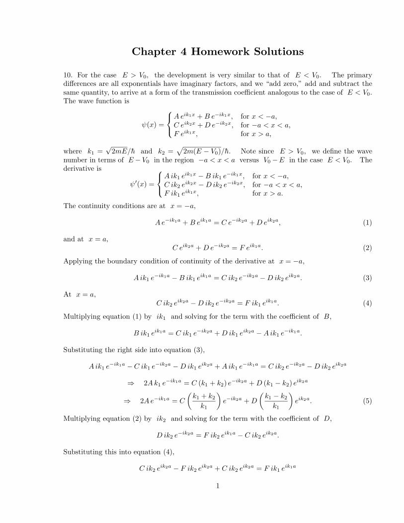
10. For the case E > V0, the development is very similar to that of E < V0. The primarydifferences are all exponentials have imaginary factors, and we “add zero,” add and subtract thesame quantity, to arrive at a form of the transmission coefficient analogous to the case of E < V0.The wave function is

ˆ(x) =

A eik1x + B e−ik1x; for x < −a,C eik2x + D e−ik2x; for −a < x < a,F eik1x; for x > a,

where k1 =√

2mE=h̄ and k2 =√

2m(E − V0)=h̄. Note since E > V0, we define the wavenumber in terms of E − V0 in the region −a < x < a versus V0 −E in the case E < V0. Thederivative is

ˆ′(x) =

Aik1 eik1x − B ik1 e−ik1x; for x < −a,C ik2 eik2x − D ik2 e−ik2x; for −a < x < a,F ik1 eik1x; for x > a.

The continuity conditions are at x = −a,

Ae−ik1a + B eik1a = C e−ik2a + D eik2a; (1)

and at x = a,C eik2a + D e−ik2a = F eik1a: (2)

Applying the boundary condition of continuity of the derivative at x = −a,

Aik1 e−ik1a − B ik1 eik1a = C ik2 e−ik2a − D ik2 eik2a: (3)

At x = a,C ik2 eik2a − D ik2 e−ik2a = F ik1 eik1a: (4)

Multiplying equation (1) by ik1 and solving for the term with the coefficient of B,

B ik1 eik1a = C ik1 e−ik2a + D ik1 eik2a − Aik1 e−ik1a:

Substituting the right side into equation (3),

Aik1 e−ik1a − C ik1 e−ik2a − D ik1 eik2a + Aik1 e−ik1a = C ik2 e−ik2a − D ik2 eik2a

⇒ 2Ak1 e−ik1a = C (k1 + k2) e−ik2a + D (k1 − k2) eik2a

⇒ 2Ae−ik1a = C

(k1 + k2

k1

)e−ik2a + D

(k1 − k2

k1

)eik2a: (5)

Multiplying equation (2) by ik2 and solving for the term with the coefficient of D,

D ik2 e−ik2a = F ik2 eik1a − C ik2 eik2a:

Substituting this into equation (4),

C ik2 eik2a − F ik2 eik2a + C ik2 eik2a = F ik1 eik1a

1

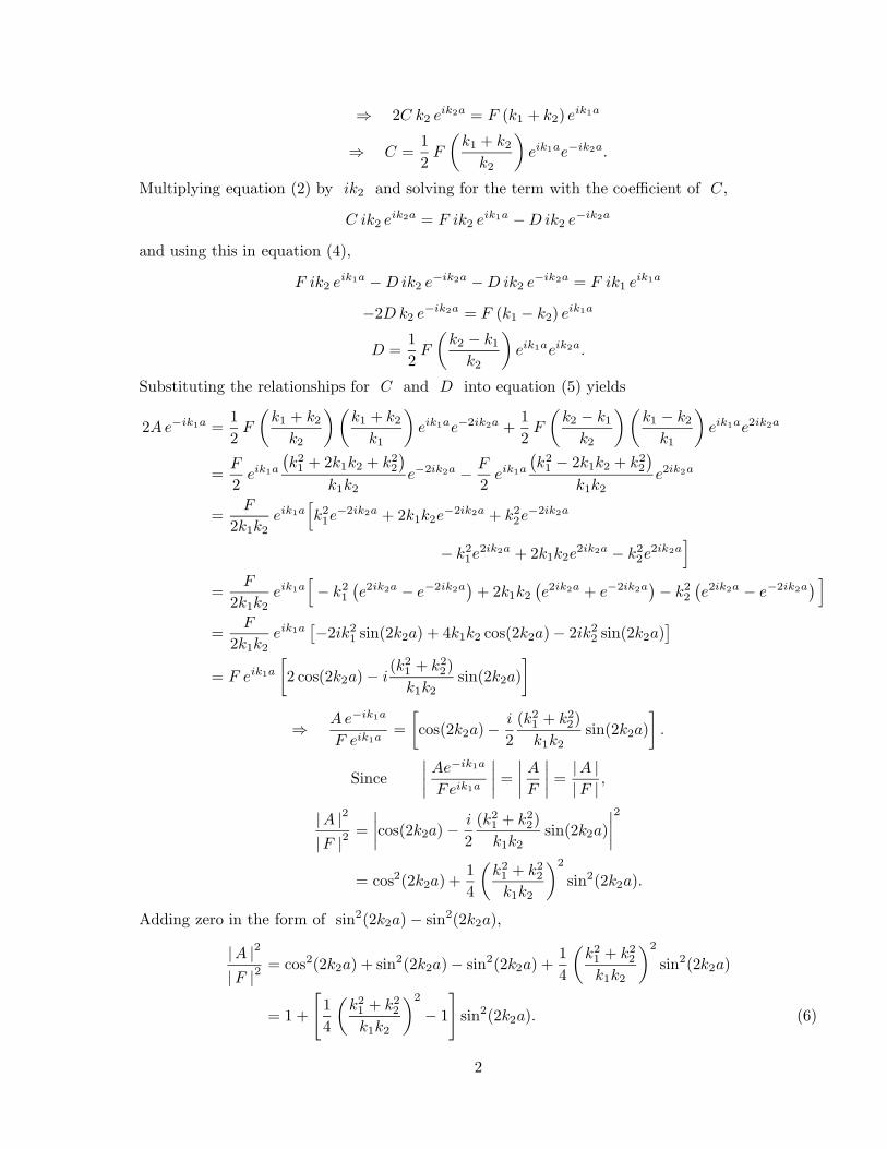
⇒ 2C k2 eik2a = F (k1 + k2) eik1a

⇒ C =12

F

(k1 + k2

k2

)eik1ae−ik2a:

Multiplying equation (2) by ik2 and solving for the term with the coefficient of C ,

C ik2 eik2a = F ik2 eik1a − D ik2 e−ik2a

and using this in equation (4),

F ik2 eik1a − D ik2 e−ik2a − D ik2 e−ik2a = F ik1 eik1a

−2D k2 e−ik2a = F (k1 − k2) eik1a

D =12

F

(k2 − k1

k2

)eik1aeik2a:

Substituting the relationships for C and D into equation (5) yields

2Ae−ik1a =12

F

(k1 + k2

k2

) (k1 + k2

k1

)eik1ae−2ik2a +

12

F

(k2 − k1

k2

) (k1 − k2

k1

)eik1ae2ik2a

=F

2eik1a

(k21 + 2k1k2 + k2

2

)

k1k2e−2ik2a − F

2eik1a

(k21 − 2k1k2 + k2

2

)

k1k2e2ik2a

=F

2k1k2eik1a

[k21e

−2ik2a + 2k1k2e−2ik2a + k2

2e−2ik2a

− k21e

2ik2a + 2k1k2e2ik2a − k2

2e2ik2a

]

=F

2k1k2eik1a

[− k2

1(e2ik2a − e−2ik2a

)+ 2k1k2

(e2ik2a + e−2ik2a

)− k2

2(e2ik2a − e−2ik2a

) ]

=F

2k1k2eik1a

[−2ik2

1 sin(2k2a) + 4k1k2 cos(2k2a) − 2ik22 sin(2k2a)

]

= F eik1a

[2 cos(2k2a) − i

(k21 + k2

2)k1k2

sin(2k2a)]

⇒Ae−ik1a

F eik1a=

[cos(2k2a) −

i

2(k2

1 + k22)

k1k2sin(2k2a)

]:

Since∣∣∣∣Ae−ik1a

Feik1a

∣∣∣∣ =∣∣∣∣A

F

∣∣∣∣ =|A || F |

;

|A |2

|F |2=

∣∣∣∣cos(2k2a) −i

2(k2

1 + k22)

k1k2sin(2k2a)

∣∣∣∣2

= cos2(2k2a) +14

(k21 + k2

2

k1k2

)2

sin2(2k2a):

Adding zero in the form of sin2(2k2a) − sin2(2k2a),

|A |2

| F |2= cos2(2k2a) + sin2(2k2a) − sin2(2k2a) +

14

(k21 + k2

2

k1k2

)2

sin2(2k2a)

= 1 +

[14

(k21 + k2

2

k1k2

)2

− 1

]sin2(2k2a): (6)

2

The expression in the square brackets reduces,

14

(k21 + k2

2

k1k2

)2

− 1 =k41 + 2k2

1k22 + k4

2

4k21k

22

−4k2

1k22

4k21k

22

=k41 − 2k2

1k22 + k4

2

4k21k

22

=14

(k21 − k2

2

k1k2

)2

:

In terms of energy where k1 =√

2mE=h̄ and k2 =√

2m(E − V0)=h̄, this is

14

2mh̄2 E − 2m

h̄2 (E − V0)

2m

h̄2

√E

√(E − V0)

2

=14

(E − E + V0√E

√(E − V0)

)2

=V 2

0

4E(E − V0):

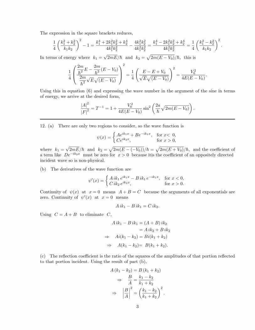
Using this in equation (6) and expressing the wave number in the argument of the sine in termsof energy, we arrive at the desired form,

|A|2

|F |2= T −1 = 1 +

V 20

4E(E − V0)sin2

(2a

h̄

√2m(E − V0)

):

12. (a) There are only two regions to consider, so the wave function is

ˆ(x) ={

Aeik1x + Be−ik1x; for x < 0,Ceik2x; for x > 0,

where k1 =√

2mE=h̄ and k2 =√

2m(E − (−V0))=h̄ =√

2m(E + V0)=h̄, and the coefficient ofa term like De−ik2x must be zero for x > 0 because it is the coefficient of an oppositely directedincident wave so is non-physical.

(b) The derivatives of the wave function are

ˆ′(x) ={

Aik1 eik1x − B ik1 e−ik1x; for x < 0,C ik2 eik2x; for x > 0.

Continuity of ˆ(x) at x = 0 means A + B = C because the arguments of all exponentials arezero. Continuity of ˆ′(x) at x = 0 means

Aik1 − B ik1 = C ik2:

Using C = A + B to eliminate C ,

Aik1 − B ik1 = (A + B) ik2

= Aik2 + B ik2

⇒ Ai(k1 − k2) = Bi(k1 + k2)

⇒ A(k1 − k2) = B(k1 + k2):

(c) The reflection coefficient is the ratio of the squares of the amplitudes of that portion reflectedto that portion incident. Using the result of part (b),

A (k1 − k2) = B (k1 + k2)

⇒ B

A=

k1 − k2

k1 + k2

⇒∣∣∣∣B

A

∣∣∣∣2

=(

k1 − k2

k1 + k2

)2

:

3

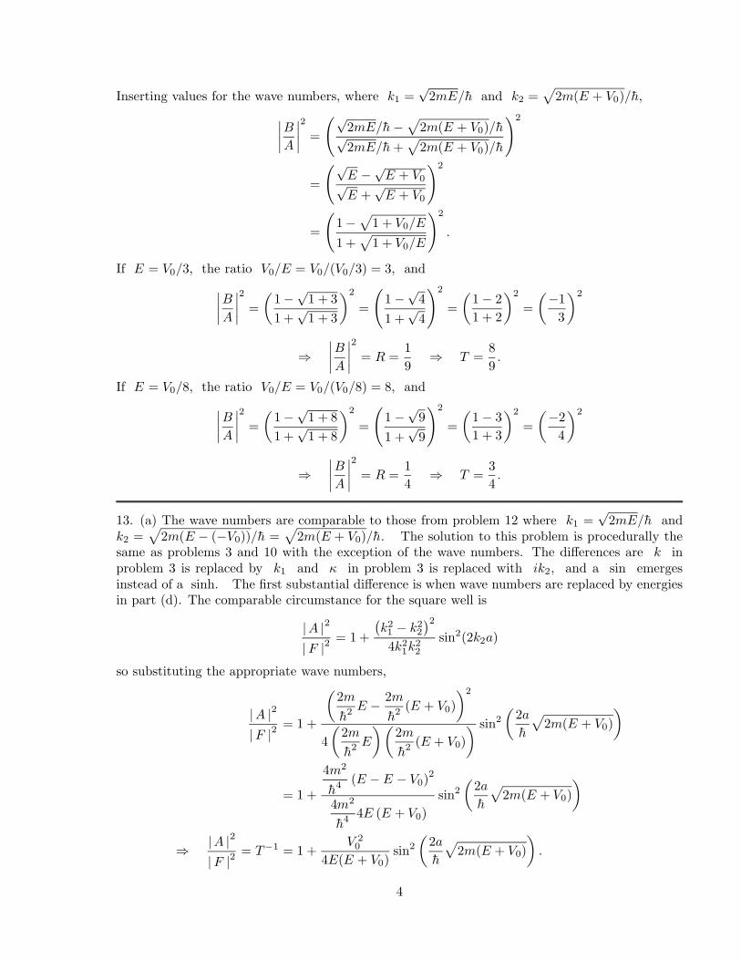
Inserting values for the wave numbers, where k1 =√

2mE=h̄ and k2 =√

2m(E + V0)=h̄,

∣∣∣∣B

A

∣∣∣∣2

=

(√2mE=h̄ −

√2m(E + V0)=h̄√

2mE=h̄ +√

2m(E + V0)=h̄

)2

=

(√E −

√E + V0√

E +√

E + V0

)2

=

(1 −

√1 + V0=E

1 +√

1 + V0=E

)2

:

If E = V0=3, the ratio V0=E = V0=(V0=3) = 3, and∣∣∣∣B

A

∣∣∣∣2

=(

1 −√

1 + 31 +

√1 + 3

)2

=

(1 −

√4

1 +√

4

)2

=(

1 − 21 + 2

)2

=(

−13

)2

⇒∣∣∣∣B

A

∣∣∣∣2

= R =19

⇒ T =89:

If E = V0=8, the ratio V0=E = V0=(V0=8) = 8, and∣∣∣∣B

A

∣∣∣∣2

=(

1 −√

1 + 81 +

√1 + 8

)2

=

(1 −

√9

1 +√

9

)2

=(

1 − 31 + 3

)2

=(

−24

)2

⇒∣∣∣∣B

A

∣∣∣∣2

= R =14

⇒ T =34:

13. (a) The wave numbers are comparable to those from problem 12 where k1 =√

2mE=h̄ andk2 =

√2m(E − (−V0))=h̄ =

√2m(E + V0)=h̄. The solution to this problem is procedurally the

same as problems 3 and 10 with the exception of the wave numbers. The differences are k inproblem 3 is replaced by k1 and • in problem 3 is replaced with ik2, and a sin emergesinstead of a sinh. The first substantial difference is when wave numbers are replaced by energiesin part (d). The comparable circumstance for the square well is

|A |2

| F |2= 1 +

(k21 − k2

2)2

4k21k

22

sin2(2k2a)

so substituting the appropriate wave numbers,

|A |2

| F |2= 1 +

(2m

h̄2 E −2m

h̄2 (E + V0))2

4(

2m

h̄2 E

)(2m

h̄2 (E + V0)) sin2

(2a

h̄

√2m(E + V0)

)

= 1 +

4m2

h̄4 (E − E − V0)2

4m2

h̄4 4E (E + V0)sin2

(2a

h̄

√2m(E + V0)

)

⇒|A |2

| F |2= T−1 = 1 +

V 20

4E(E + V0)sin2

(2a

h̄

√2m(E + V0)

):

4

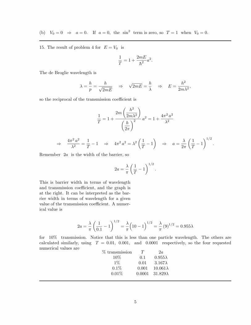
(b) V0 = 0 ⇒ a = 0. If a = 0, the sin2 term is zero, so T = 1 when V0 = 0.

15. The result of problem 4 for E = V0 is

1T

= 1 +2mE

h̄2 a2:

The de Broglie wavelength is

‚ =h

p=

h√2mE

⇒√

2mE =h

‚⇒ E =

h2

2m‚2 ;

so the reciprocal of the transmission coefficient is

1T

= 1 +2m

(h2

2m‚2

)

(h

2…

)2 a2 = 1 +4…2 a2

‚2

⇒4…2 a2

‚2 =1T

− 1 ⇒ 4…2 a2 = ‚2(

1T

− 1)

⇒ a =‚

2…

(1T

− 1)1=2

:

Remember 2a is the width of the barrier, so

2a =‚

…

(1T

− 1)1=2

:

This is barrier width in terms of wavelengthand transmission coefficient, and the graph isat the right. It can be interpreted as the bar-rier width in terms of wavelength for a givenvalue of the transmission coefficient. A numer-ical value is

2a =‚

…

(1

0:1− 1

)1=2

=‚

…

(10 − 1

)1=2=

‚

…(9)1=2 = 0:955‚

for 10% transmission. Notice that this is less than one particle wavelength. The others arecalculated similarly, using T = 0:01; 0:001, and 0:0001 respectively, so the four requestednumerical values are

% transmission T 2a10% 0:1 0:955‚1% 0:01 3:167‚

0:1% 0:001 10:061‚0:01% 0:0001 31:829‚

5