saving electrical energy in commercial buildings -...

Saving Electrical Energy inCommercial Buildings

by

Ryan Case

A thesispresented to the University of Waterloo

in fulfillment of thethesis requirement for the degree of

Master of Mathematicsin

Computer Science

Waterloo, Ontario, Canada, 2012

c© Ryan Case 2012

I hereby declare that I am the sole author of this thesis. This is a true copy of the thesis,including any required final revisions, as accepted by my examiners.

I understand that my thesis may be made electronically available to the public.

ii

Abstract

With the commercial and institutional building sectors using approximately 29% and 34%of all electrical energy consumption in Canada and the United States, respectively, savingelectrical energy in commercial and institutional buildings represents an important chal-lenge for both the environment and the energy consumer. Concurrently, a rapid decline inthe cost of microprocessing and communication has enabled the profileration of smart me-ters, which allow a customer to monitor energy usage every hour, 15 minutes or even everyminute. Algorithmic analysis of this stream of meter readings would allow 1) a buildingoperator to predict the potential cost savings from implemented energy savings measureswithout engaging the services of an expensive energy expert; and 2) an energy expert toquickly obtain a high-level understanding of a building’s operating parameters without atime-consuming and expensive site visit. This thesis develops an algorithm that takes asinput a stream of building meter data and outputs a building’s operating parameters. Thisoutput can be used directly by an energy expert to assess a building’s performance; itcan also be used as input to other algorithms or systems, such as systems that 1) predictthe cost savings from a change in these operating parameters; 2) benchmark a portfolio ofbuilding; 3) create baseline models for measurement and verification programs; 4) detectanomalous building behaviour; 5) provide novel data visualization methods; or 6) assessthe applicability of demand response programs on a given building. To illustrate this, weshow how operating parameters can be used to estimate potential energy savings fromenergy savings measures and predict building energy consumption. We validate our ap-proach on a range of commercial and institutional buildings in Canada and the UnitedStates; our dataset consists of 10 buildings across a variety of geographies and industriesand comprises over 21 years of meter data. We use K-fold cross-validation and benchmarkour work against a leading black-box prediction algorithm; our model offers comparableprediction accuracy while being far less complex.

iii

Acknowledgements

I would like to thank my advisor, Dr. S. Keshav, for his patient support, criticism andadvice throughout my graduate studies. His commitment to the success of his studentsgoes far beyond his professional duties; I consider myself very fortunate to have had himas an advisor.

I wish to thank my co-supervisor, Dr. Catherine Rosenberg, for providing useful sug-gestions, input and feedback throughout my research, and to Dr. Ian Rowlands and Dr.Daniel Lizotte for serving as readers for my thesis.

I owe a great intellectual debt to the people at Pulse Energy; their input and contri-butions formed the foundation of this thesis. I benefited greatly from conversations withOwen Rogers, Chris Porter, Jason Kok, James Christopherson, Kevin Tate, Brent Bowker,Neil Gentleman, Chuck Clark, Craig Handley and undoubtedly many others to whom Iapologize for their omission.

iv

Dedication

To my parents.

v

Table of Contents

List of Tables viii

List of Figures ix

1 Introduction 1

1.1 Definitions . . . . . . . . . . . . . . . . . . . . . . . . . . . . . . . . . . . . 1

1.2 Building Operating Modes . . . . . . . . . . . . . . . . . . . . . . . . . . . 3

1.3 Stakeholders . . . . . . . . . . . . . . . . . . . . . . . . . . . . . . . . . . . 3

1.4 Problem Statement . . . . . . . . . . . . . . . . . . . . . . . . . . . . . . . 6

1.5 Assumptions . . . . . . . . . . . . . . . . . . . . . . . . . . . . . . . . . . . 8

1.6 Solution Overview . . . . . . . . . . . . . . . . . . . . . . . . . . . . . . . 8

1.7 Thesis Organization . . . . . . . . . . . . . . . . . . . . . . . . . . . . . . . 8

2 Related Work 9

3 Enerlytic 13

3.1 Summarizing . . . . . . . . . . . . . . . . . . . . . . . . . . . . . . . . . . 19

3.2 Labelling . . . . . . . . . . . . . . . . . . . . . . . . . . . . . . . . . . . . . 19

3.3 Regression . . . . . . . . . . . . . . . . . . . . . . . . . . . . . . . . . . . . 20

3.4 Prediction . . . . . . . . . . . . . . . . . . . . . . . . . . . . . . . . . . . . 22

3.5 ESM Estimation . . . . . . . . . . . . . . . . . . . . . . . . . . . . . . . . 24

3.6 Concluding Remarks . . . . . . . . . . . . . . . . . . . . . . . . . . . . . . 25

vi

4 Evaluation 29

4.1 Results . . . . . . . . . . . . . . . . . . . . . . . . . . . . . . . . . . . . . . 30

5 Implementation 54

6 Conclusion 59

6.1 Limitations . . . . . . . . . . . . . . . . . . . . . . . . . . . . . . . . . . . 60

6.2 Future Work . . . . . . . . . . . . . . . . . . . . . . . . . . . . . . . . . . . 61

References 62

APPENDICES 66

A Description of the Dataset 67

vii

List of Tables

3.1 Regression parameter definitions. . . . . . . . . . . . . . . . . . . . . . . . 20

3.2 Acceptable piecewise parameter ranges . . . . . . . . . . . . . . . . . . . . 22

A.1 Description of the dataset . . . . . . . . . . . . . . . . . . . . . . . . . . . 67

viii

List of Figures

1.1 Load Profile . . . . . . . . . . . . . . . . . . . . . . . . . . . . . . . . . . . 2

1.2 Load Profiles and Operating Modes . . . . . . . . . . . . . . . . . . . . . . 4

1.3 Goal of the Thesis . . . . . . . . . . . . . . . . . . . . . . . . . . . . . . . 7

2.1 Energy Signature . . . . . . . . . . . . . . . . . . . . . . . . . . . . . . . . 11

3.1 Summarizing . . . . . . . . . . . . . . . . . . . . . . . . . . . . . . . . . . 14

3.2 Enerlytic Algorithm 1 . . . . . . . . . . . . . . . . . . . . . . . . . . . . . 15




3.6 Piecewise Linear Regression Parameters . . . . . . . . . . . . . . . . . . . 21

3.7 Prediction Overview . . . . . . . . . . . . . . . . . . . . . . . . . . . . . . 23

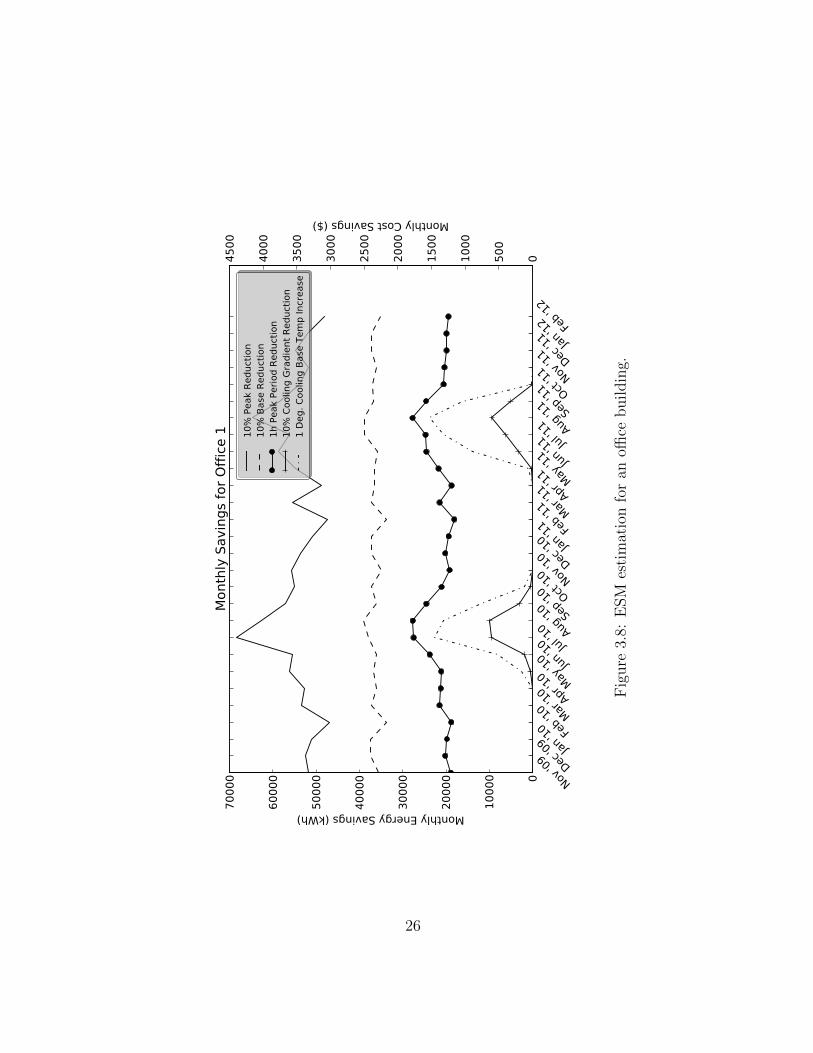
3.8 ESM Estimation Example (Office) . . . . . . . . . . . . . . . . . . . . . . . 26

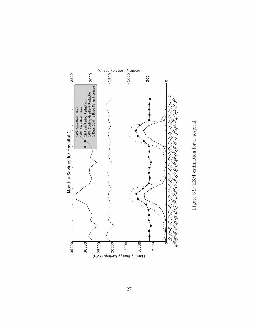
3.9 ESM Estimation Example (Hospital) . . . . . . . . . . . . . . . . . . . . . 27

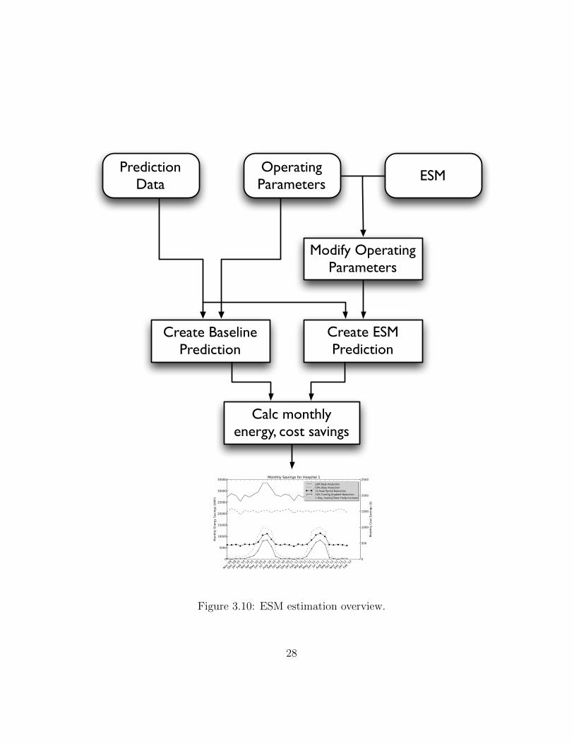
3.10 ESM Estimation Overview . . . . . . . . . . . . . . . . . . . . . . . . . . . 28

4.1 CV-RMSE Results . . . . . . . . . . . . . . . . . . . . . . . . . . . . . . . 31

4.2 Mean Bias Error Results . . . . . . . . . . . . . . . . . . . . . . . . . . . . 32

4.3 Office 1 Actual and Predicted Demand . . . . . . . . . . . . . . . . . . . . 34

4.4 Office 1 Training and Residual Demand . . . . . . . . . . . . . . . . . . . . 35

4.5 Office 1 Weekday Energy Signatures . . . . . . . . . . . . . . . . . . . . . . 36

ix

4.6 Office 1 Weekend Energy Signatures . . . . . . . . . . . . . . . . . . . . . . 37

4.7 School 1 Actual and Predicted Demand . . . . . . . . . . . . . . . . . . . . 38

4.8 School 1 Training and Residual Demand . . . . . . . . . . . . . . . . . . . 39

4.9 School 1 Weekday Energy Signatures . . . . . . . . . . . . . . . . . . . . . 40

4.10 School 1 Weekend Energy Signatures . . . . . . . . . . . . . . . . . . . . . 41

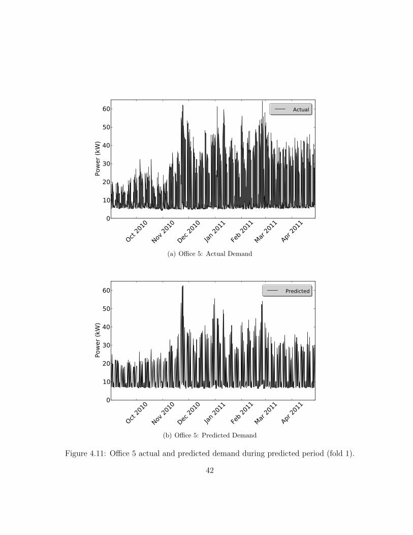
4.11 Office 5 Actual and Predicted Demand . . . . . . . . . . . . . . . . . . . . 42

4.12 Office 5 Training and Residual Demand . . . . . . . . . . . . . . . . . . . . 43

4.13 Office 5 Weekday Energy Signatures . . . . . . . . . . . . . . . . . . . . . . 44

4.14 Office 5 Weekend Energy Signatures . . . . . . . . . . . . . . . . . . . . . . 45

4.15 Office 3 Actual and Predicted Demand (Fold 1) . . . . . . . . . . . . . . . 46

4.16 Office 3 Training and Residual Demand (Fold 1) . . . . . . . . . . . . . . . 47

4.17 Office 3 Weekday Energy Signatures (Fold 1) . . . . . . . . . . . . . . . . . 48

4.18 Office 3 Weekend Energy Signatures (Fold 1) . . . . . . . . . . . . . . . . . 49

4.19 Office 3 Actual and Predicted Demand (Fold 2) . . . . . . . . . . . . . . . 50

4.20 Office 3 Training and Residual Demand (Fold 2) . . . . . . . . . . . . . . . 51

4.21 Office 3 Weekday Energy Signatures (Fold 2) . . . . . . . . . . . . . . . . . 52

4.22 Office 3 Weekend Energy Signatures (Fold 2) . . . . . . . . . . . . . . . . . 53

5.1 Implementation Architecture . . . . . . . . . . . . . . . . . . . . . . . . . . 55

5.2 Web UI Home . . . . . . . . . . . . . . . . . . . . . . . . . . . . . . . . . . 56

5.3 Web UI Plot Selector . . . . . . . . . . . . . . . . . . . . . . . . . . . . . . 57

5.4 Web UI Plot Viewer . . . . . . . . . . . . . . . . . . . . . . . . . . . . . . 58

x

Chapter 1

Introduction

Three hundred and fifty three billion dollars (U.S.) was spent on 3,724 TWh of electricity inthe United States in 2009 [1]. In Canada during the same year, approximately 500 TWh ofelectricity was consumed, producing a total of 85.61 megatonnes of carbon dioxide [2] [3].With commercial and institutional buildings responsible for 29% of 2009 electricity usein Canada [2] and 34% in the United States [1], saving energy in the commercial andinstitutional building sectors represents an important challenge for both the environmentand the energy consumer.

This challenge coincides with the rapid decline in the cost of microprocessing andcommunication that has enabled the recent proliferation of advanced (“smart”) meter-ing infrastructure: as of 2010, approximately 14% of residential and 11% of commercialcustomers had smart meter installations in the United States [4]. In Ontario alone, 3.36million customers out of a total of 4.75 million had smart meters in 2009, with the installedcapacity rising to 4.57 million by 2010 [5]. Instead of receiving a consolidated bill from theutility each month, the customer can now learn of his or her usage every hour, every 15minutes or even every minute. We believe an algorithmic analysis of this stream of meterreadings can enable energy savings in commercial and institutional buildings. This thesiscontains the development, validation and results of such analysis.

1.1 Definitions

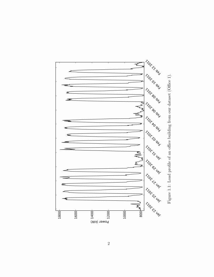
We define the output of a stream of meter readings to be meter data, a plot of meterdata over time to be a load profile, and a load profile over the course of one day to be

1

Jan

23 2

011

Jan

25 2

011

Jan

27 2

011

Jan

29 2

011

Jan

31 2

011

Feb

02 2

011 Fe

b 04

201

1 Feb

06 2

011 Fe

b 08

201

1 Feb

10 2

011 Fe

b 12

201

1

80

0

10

00

12

00

14

00

16

00

18

00

Power (kW)

Fig

ure

1.1:

Loa

dpro

file

ofan

office

buildin

gfr

omou

rdat

aset

(Offi

ce1)

.

2

a daily load profile. Consider the load profile in Figure 1.1. This building’s daily loadprofile is relatively consistent during each weekday, and assumes a different shape on theweekend. If this sample is an indication of the building’s overall electrical energy con-sumption pattern, then the building appears to have two operating modes, or groups ofdays which, given the same weather pattern, have similar daily load profiles. Recognizingoperating modes is fundamental to understanding the building’s energy consumption pat-terns, and can be used to identify energy savings measures (ESMs). ESMs are actionableitems which can be undertaken to conserve electrical energy in a building. Categories ofESMs are retrofits (upgrading equipment), operational (changing equipment operation),or behavioural (changing the occupants’ behaviour). The process of undertaking ESMsinvolves several stakeholders, which we discuss in Section 1.3.

1.2 Building Operating Modes

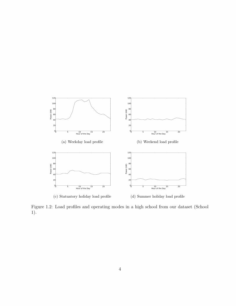
Consider Figure 1.2, which shows different daily load profiles. Are there four modes ofoperation, or three? Identifying the operating modes of a building is an ill-posed clusteringproblem. Arguably there are three modes, implying the statuatory holiday is in the samemode as the weekend. This in itself may be an insight: how similar are statuatory holidaysto weekends from the perspective of energy consumption? The statuatory holiday in thiscase is similar to the weekend, but there is a deviation in demand during the morning.Identifying the root cause of this difference could lead to an energy savings opportunity.

1.3 Stakeholders

The process of saving electrical energy in commercial and industrial buildings in the UnitedStates and Canada can involve many roles and stakeholders, each of which may be fulfilledby separate, or even multiple, parties. The following is a list of roles that may be filledduring the energy saving process:

• Meter operator: installs and maintains the metering equipment.

• Data warehouse: stores and provides access to the meter data.

• Building operator: maintains the building, its equipment, and manages the corre-sponding budget.

3

0 5 10 15 20Hour of the Day

0

20

40

60

80

100

120

Pow

er

(kW

)

(a) Weekday load profile


0

20

40

60

80

100

120

Pow

er

(kW

)

(b) Weekend load profile


0

20

40

60

80

100

120

Pow

er

(kW

)

(c) Statuatory holiday load profile


0

20

40

60

80

100

120

Pow

er

(kW

)

(d) Summer holiday load profile

Figure 1.2: Load profiles and operating modes in a high school from our dataset (School1).

4

• Energy expert: uses its domain knowledge, proprietary tools, tools provided by thesoftware provider, and knowledge of the building provided by the building operatorto create a list of candidate ESMs or “recommendations” for the building operator.

• Software provider: provides software tools for meter data visualization, analysis andreporting for use by energy experts or building operators.

• ESM implementor: implements the chosen ESM(s).

We assume any omitted roles will have a negligible effect on the discussion. Examplesof omitted roles could be the owner of the building, or the party which evaluates the resultsof the ESM.

We illustrate how these roles might be fulfilled with an example: a case study [6]from B.C. Hydro’s “Continuous Optimization” program [7]. This program focuses on re-commissioning and improving efficiency in commercial buildings:

• Meter operator: B.C. Hydro, a Canadian electric utility, upgrades metering equip-ment at the building and connects the meter to its metering infrastructure; alterna-tively the building operator installs the meter if a BC Hydro meter is not already inplace [8].

• Data warehouse: BC Hydro accesses the data through its metering infrastructure;alternatively, the customer may be required to provide data collection services, eg.through their Internet connection. The data is then stored and used by the energyexpert or software provider, and potentially by BC Hydro itself.

• Building operator: Jawl Properties, who also own the building(s)

• Energy expert: SES Consulting

• Software provider: SES Consulting, sub-contracts the software requirements to PulseEnergy

• ESM implementor: SES Consulting oversees the implementation process, which ispaid for by the building operator

5

1.4 Problem Statement

The current practice for identifying energy savings involves two primary parties: 1) buildingoperators, who have a deep knowledge of the building’s operation but lack the resources,such as time or expertise, to investigate energy savings; and 2) energy experts, who provideexpertise and resources as a service, and may lack detailed knowledge of how a particularbuilding is run. We propose to analyze a stream of meter readings that would allow:

1. A building operator to determine the potential cost savings from implementatingenergy savings measures (ESMs) without engaging the services of an expensive energyexpert

2. An energy expert to quickly obtain a high-level understanding of a building’s oper-ating parameters without a time-consuming and expensive site visit

Therefore, although the selection of appropriate ESMs for a particular building requires adegree of understanding of its operations that is beyond the scope of this work, we believethat there are still substantial benefits from an algorithmic approach to meter stream dataanalysis.

Importantly, such an approach must take into account the fact that a building oper-ates in one of several modes, and that its energy consumption varies dramatically withoperating mode. Moreover, the approach must model building energy use in terms ofhuman-understandable operating parameters (such as base and peak load as a function ofthe ambient temperature) so that an energy expert can assess the gains from changes inthese operating parameters due to an ESM. These two criteria serve to motivate the workpresented in this thesis.

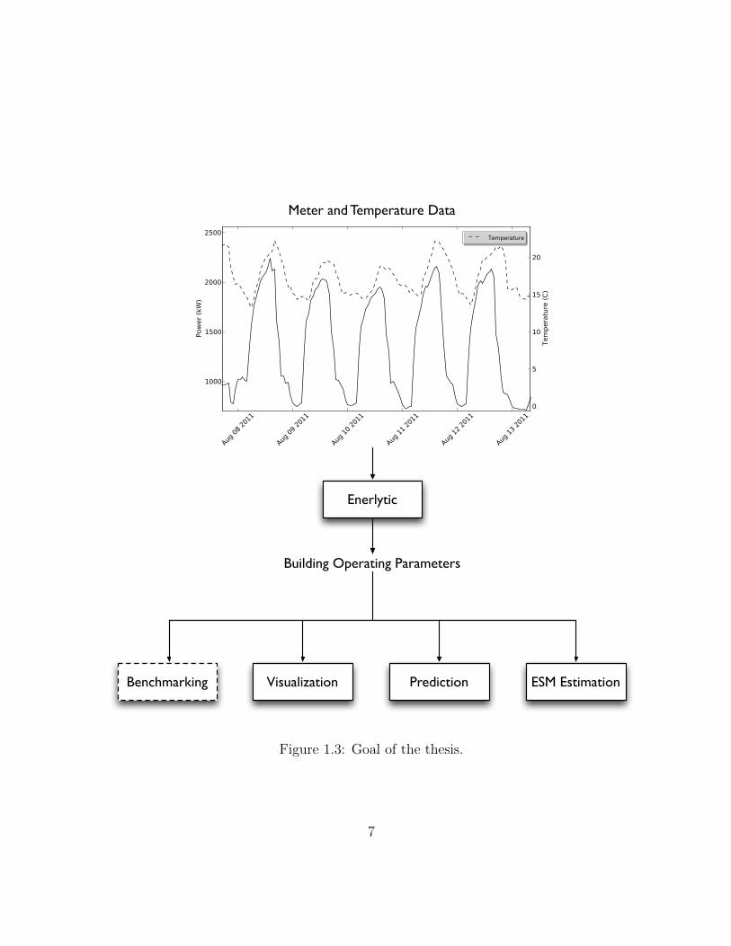
In summary, the goal of this thesis, as illustrated in Figure 1.3 is to develop an algorithmthat takes as input a stream of building meter data and that outputs the building’s operat-ing parameters. This output can be used directly by an energy expert to rapidly assess thebuilding’s performance. It can also be used as input to other systems, for example systemsthat 1) predict the cost savings from a change in these operating parameters; 2) bench-mark a portfolio of building; 3) create baseline models for measurement and verificationprograms; 4) detect anomalous building behaviour; 5) provide novel data visualizationmethods; or 6) assess the applicability of demand response programs on a given building.

6

Meter and Temperature Data

Enerlytic

ESM EstimationBenchmarking Visualization Prediction

Building Operating Parameters

Figure 1.3: Goal of the thesis.

7

1.5 Assumptions

We assume that:

1. For sake of simplicity, meter readings are taken at an hourly interval. There are notechnical limitations preventing this work to being extended to meter readings atother intervals.

2. The outdoor weather can be approximated with hourly dry-bulb temperature mea-surements from a nearby weather station.

3. If the building parameters are being used for prediction, temperature data can alsobe predicted for the corresponding period.

4. Predictions need not be made for operating modes that are not in the input data

1.6 Solution Overview

We propose an algorithm, Enerlytic, which partitions meter data into operating modesusing a process we call labelling, and creates a model of a building’s electrical energyuse during each operating mode as a function of the outdoor air temperature. The modelparameters are amenable to human interpretation. We develop a novel algorithm to extractthe peak and base periods of each day, and model these loads as a function of the outdoortemperature using piecewise linear regressions. We validate the output of Enerlytic, thebuilding’s operating parameters, by using them to predict over 21 years of meter data on10 different buildings across North America. Our prediction accuracy is comparable to acompetitive black-box method [9]. We also show how these operating parameters can beused as input to other algorithms, for example to estimate the potential for energy savingsin a building.

1.7 Thesis Organization

In Chapter 2 we provide an overview of the related literature. Chapter 3 describes thedevelopment of our solution, and Chapter 4 discusses the results. Chapter 5 providesadditional discussion, and Chapter 6 provides concluding remarks, as well as limitationsto our solution and areas of future work.

8

Chapter 2

Related Work

This thesis develops an algorithm that takes as input a stream of building meter data andoutputs a model which can provide an energy expert with a high-level understanding of abuilding. The output also serves as input to other algorithms, for example for estimatingthe potential cost savings from implementing energy savings measures, or for predicting abuilding’s energy use. We now survey prior work with similar goals.

Advanced tools for building modelling and simulation, such as EnergyPlus [10] [11] arewell established in the building design and efficiency community. These tools are usefulfor advanced analysis of building energy consumption, particularly when no meter datais available. However, their complexity and need for physical building data make themdifficult to calibrate [12] and ill-suited to meet our goals.

Creating energy models from meter data and weather parameters—such as temperatureand humidity—for predicting energy consumption has also been well studied. This problemwas investigated in detail for the 1993 ASHRAE “Great Energy Predictor Shootout” [13],which resulted in many robust methods for predicting energy use. Some entries, such as thewinning entry from David MacKay [14], involved systems to determine which inputs weremost relevant for accurate prediction, illustrating possible correlations between inputs andoutput. Many of the top performers, including the winning entry, are neural-network-basedmodels that provide little insight into the building’s energy consumption patterns. Theblack-box nature of these prediction algorithms make them unsuitable for our purpose;however, we use a more recently developed black-box prediction model for benchmarkingthe prediction accuracy of our work. This model is based on kernel regression [9], andperforms comparably to the top prediction models in the ASHRAE shootout based onprediction accuracy.

9

“Grey-box” models, which contrast with “black-box” models, use the most similar ap-proach to our own. These models use parameters that are related to the physics of thebuilding or its energy consumption patterns. Some, like Lee and Brown [15], do not usemeter data as input but instead require other parameters of the physical building, suchas the floor plan. Others use well established methodology for fitting piecewise linear re-gression models to the relationship between outdoor dry-bulb air temperature and averagedaily energy consumption; for example, the work by Kissock et al [16]. The piecewiselinear regression model fits two linear regressions which are continuous at a single change-point—the point where one regression changes to the other, as illustrated in Figure 2.1.The resulting regression is in a shape similar to a hockey stick, with the bend occurringat the change-point. If a building has electric heating or cooling, a building’s energyconsumption follows a linear or uncorrelated relationship with outdoor temperature untilsome temperature, known as the “base temperature” is reached, and then this relation-ship changes, becoming strongly correlated with temperature. The base temperature hasa direct relationship with the set point of the building’s heating or cooling system, so thiscan be a useful parameter to identify. Further, the slopes of the regressions indicate theincrease in the amount of energy expended per degree increase in the outdoor air temper-ature. These slopes, known as the heating and cooling gradients, serve to identify physicalelements of the building, such as thermal components (the building envelope, and heatingand cooling systems).

Sever et al [17] show how grey box models can be used to estimate energy savings frommodel parameters. However, they make two assumptions that are not compatible with ourgoals. First, the building is assumed to have a single operating mode. This dramaticallylimits the insight which the model can provide, since it does not capture this fundamentalaspect of the building’s energy consumption. Second, and most importantly, their modelinput is the average daily energy consumption as opposed to hourly data. This preventsanalysis of the daily load profile, such as the identification of peak or base periods, andmakes it impossible, for example, to estimate the energy savings due to an adjustment inthe average peak load or by shortening the peak load period.

Other grey-box methods also identify the peak or base periods (or “occupied and un-occupied” periods) but do not derive insight from the building’s energy consumption withtemperature, limiting the insight the models are able to provide. Mathieu et al [18] predicthourly power using a time-of-week indicator variable and either a linear or local linearregression with outdoor temperature. They demonstrate how their model can be used toestimate the effectiveness of different demand-response strategies through peak-load shift-ing. However, there are several limitations in their work. The user must manually separatea building’s “occupied” mode from its “unoccupied” mode. There is no modelling of the

10

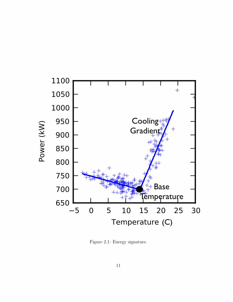
BaseTemperature

CoolingGradient

(C)

Figure 2.1: Energy signature.

11

different operating modes of the building, and the temperature modelling cannot be usedto estimate energy savings.

Cherkassky et al [19] cluster a building’s daily load profile into four periods, then useeither a bin-based [20] or non-linear regression with temperature data to predict futureconsumption. They also separate weekends from weekdays to improve the accuracy oftheir predictions, thus identifying different operating modes in the two buildings in theirtest set. However, although the output of their model could potentially be adapted toprovide some insight into the building’s energy consumption patterns, it is not clear howto manipulate such a model to obtain energy savings estimates or use it as input for othersystems.

In summary, although there is no prior work which is directly suitable for our problemstatement, our work does extend several prior approaches. We partition the daily load pro-file similar to Cherkassky et al [19], but instead of using Lloyd’s algorithm [21] we developnon-iterative algorithm. We use temperature models like those proposed by Kissock etal [16] for estimating energy savings like Sever et al [17]. The output of our algorithm canbe used as an input for estimating energy savings opportunities such as demand response,like Mathieu et al [18]. We now discuss the development of our algorithm, Enerlytic, whichmakes use of these concepts.

12

Chapter 3

Enerlytic

This chapter describes Enerlytic, an algorithm that takes as input hourly meter data andoutputs a building’s operating parameters. These parameters can be used by an energyexpert to quickly gain a high-level understanding of a building’s electrical energy consump-tion, and can be used as input to other algorithms and systems.

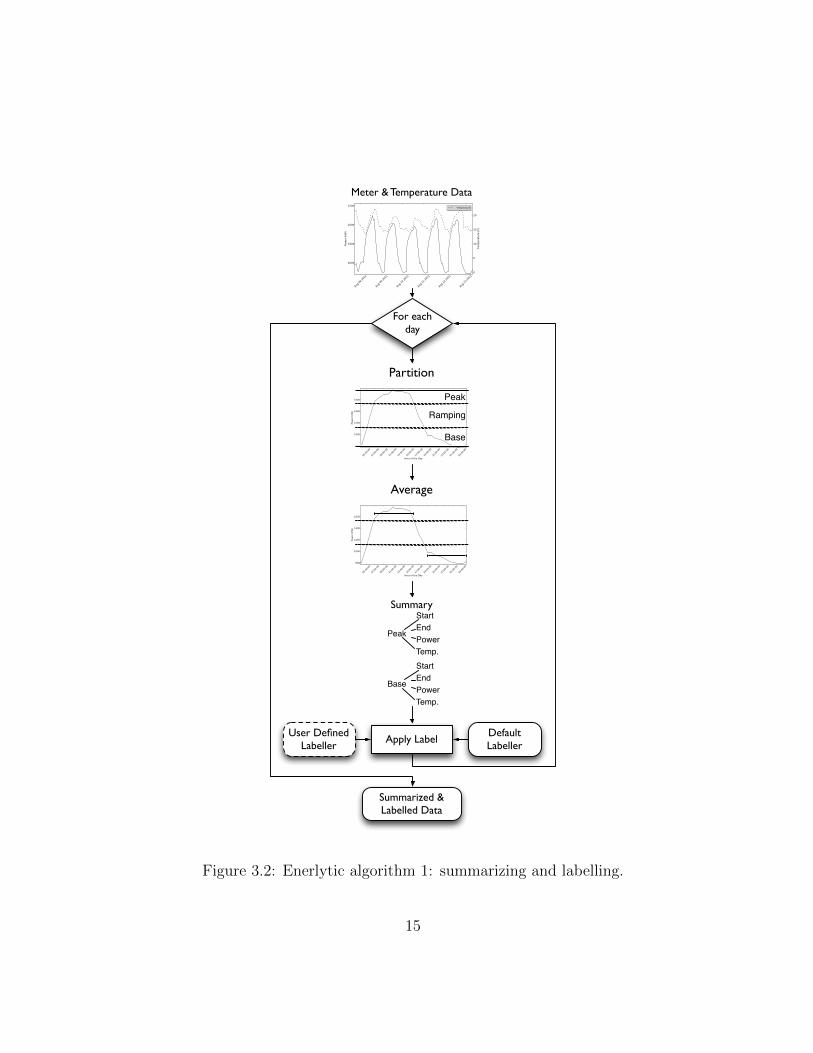
Enerlytic obtains information about a building’s operating modes through a labeller—afunction that maps a date into an operating mode based on a set of rules. If no labelleris given, Enerlytic uses a default labeller that labels weekdays and weekends; Enerlyticpartitions the days in the meter data based on their operating mode. Enerlytic modelshourly power consumption as a function of outdoor air temperature using piecewise linearregressions and a pre-processing algorithm we call summarizing. Summarizing divides eachdaily load profile into peak, base, and ramping periods and computes the mean of the peakand base periods, ignoring the ramping period. This acts as a de-noising process, which isillustrated in Figure 3.1.

Enerlytic runs an outlier detection algorithm to verify that the labelling process ade-quately partitioned the building’s operating modes for the subsequent regression fitting.This removes the outliers and alerts the expert that outliers were removed. We use theoutput of Enerlytic, the building’s operating parameters, to create predictions and esti-mate energy savings in Sections 3.4 and 3.5, respectively. The entire Enerlytic algorithmis displayed in Figures 3.2-3.5.

13

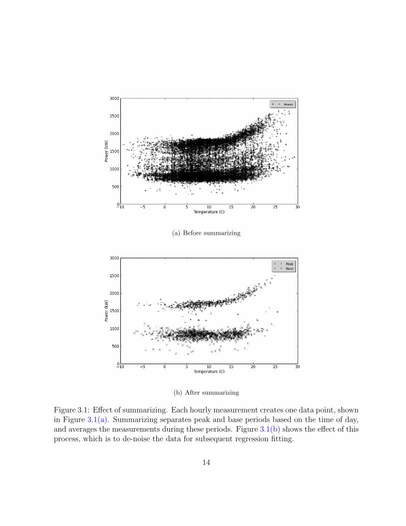
(a) Before summarizing

(b) After summarizing

Figure 3.1: Effect of summarizing. Each hourly measurement creates one data point, shownin Figure 3.1(a). Summarizing separates peak and base periods based on the time of day,and averages the measurements during these periods. Figure 3.1(b) shows the effect of thisprocess, which is to de-noise the data for subsequent regression fitting.

14

Meter & Temperature Data

For eachday

Partition

Peak

Ramping

Base

Average

User Defined Labeller

Apply LabelDefault Labeller

Summarized & Labelled Data

Peak

StartEndPowerTemp.

Base

StartEndPowerTemp.

Summary

Figure 3.2: Enerlytic algorithm 1: summarizing and labelling.

15

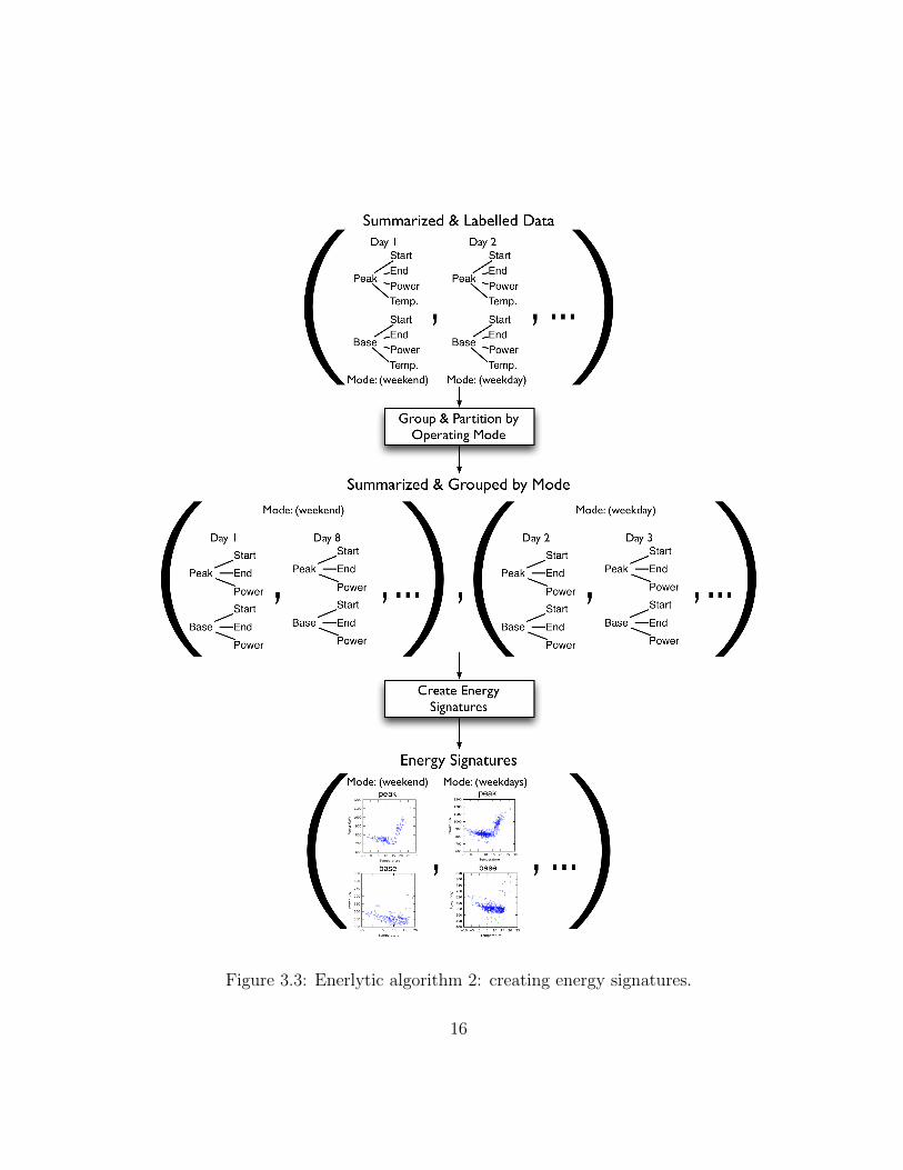
Figure 3.3: Enerlytic algorithm 2: creating energy signatures.

16

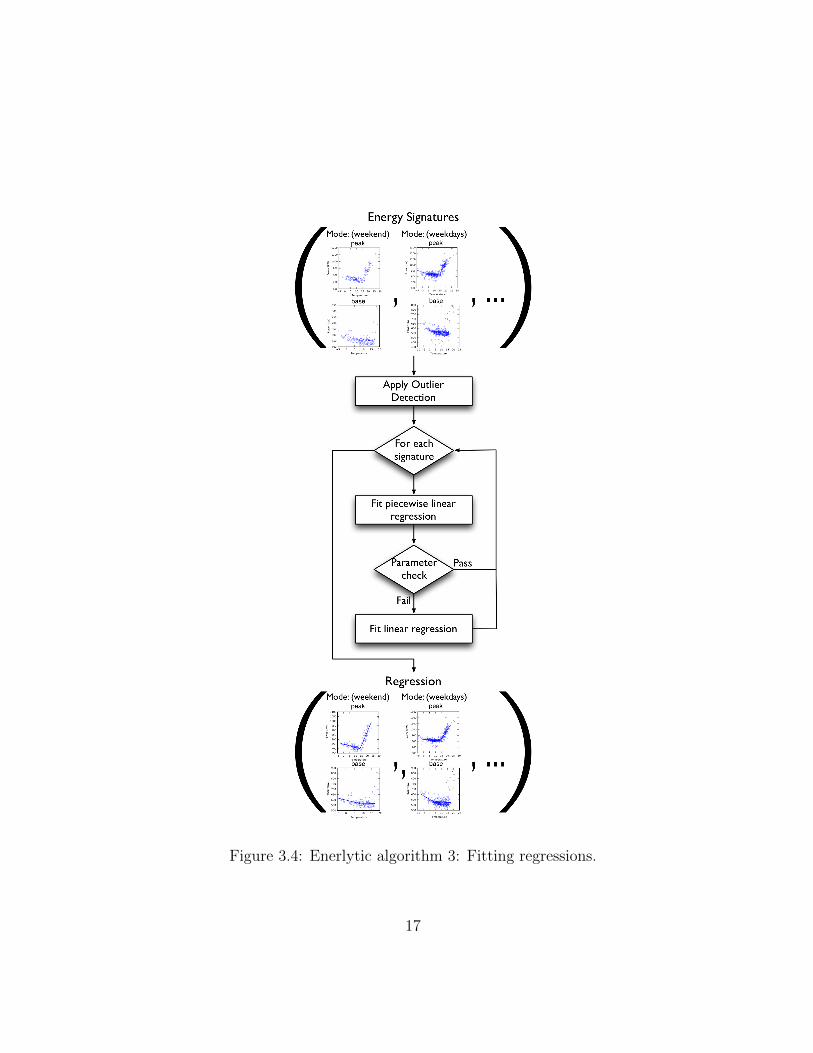
Figure 3.4: Enerlytic algorithm 3: Fitting regressions.

17

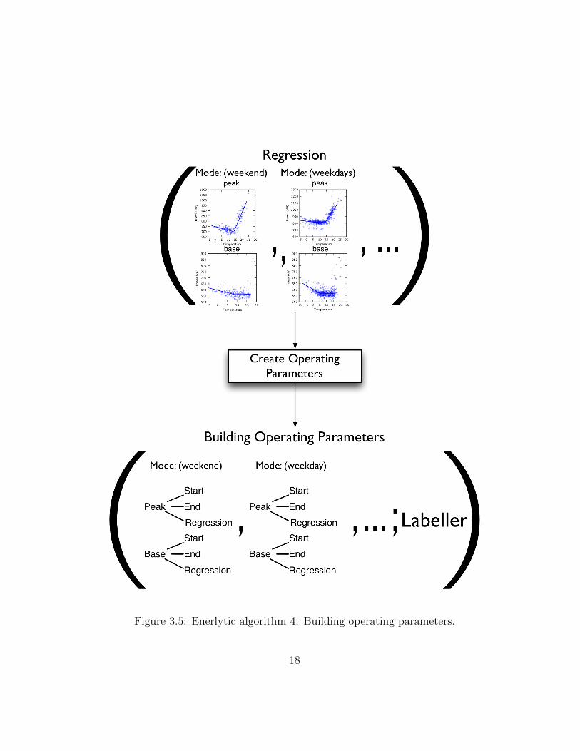
Figure 3.5: Enerlytic algorithm 4: Building operating parameters.

18

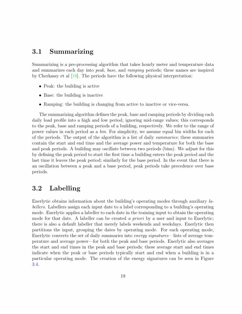
3.1 Summarizing

Summarizing is a pre-processing algorithm that takes hourly meter and temperature dataand summarizes each day into peak, base, and ramping periods; these names are inspiredby Cherkassy et al [19]. The periods have the following physical interpretation:

• Peak: the building is active

• Base: the building is inactive

• Ramping: the building is changing from active to inactive or vice-versa.

The summarizing algorithm defines the peak, base and ramping periods by dividing eachdaily load profile into a high and low period, ignoring mid-range values; this correspondsto the peak, base and ramping periods of a building, respectively. We refer to the range ofpower values in each period as a bin. For simplicity, we assume equal bin widths for eachof the periods. The output of the algorithm is a list of daily summaries ; these summariescontain the start and end time and the average power and temperature for both the baseand peak periods. A building may oscillate between two periods (bins). We adjust for thisby defining the peak period to start the first time a building enters the peak period and thelast time it leaves the peak period; similarly for the base period. In the event that there isan oscillation between a peak and a base period, peak periods take precedence over baseperiods.

3.2 Labelling

Enerlytic obtains information about the building’s operating modes through auxiliary la-bellers. Labellers assign each input date to a label corresponding to a building’s operatingmode. Enerlytic applies a labeller to each date in the training input to obtain the operatingmode for that date. A labeller can be created a priori by a user and input to Enerlytic;there is also a default labeller that merely labels weekends and weekdays. Enerlytic thenpartitions the input, grouping the dates by operating mode. For each operating mode,Enerlytic converts the set of daily summaries into energy signatures—lists of average tem-perature and average power—for both the peak and base periods. Enerlytic also averagesthe start and end times in the peak and base periods; these average start and end timesindicate when the peak or base periods typically start and end when a building is in aparticular operating mode. The creation of the energy signatures can be seen in Figure3.4.

19

Table 3.1: Regression parameter definitions.

Parameter Definition

β Y-interceptTb Base temperaturemh Heating gradientmc Cooling gradientmn Neutral gradient

3.3 Regression

If the data is not partitioned appropriately, Enerlytic may fit regressions incorrectly due toSimpson’s Paradox [22]. If two separate populations are combined because of inadequatepartitioning, for example, due to inadequate labelling, the apparent correlation betweentemperature and power may be distorted. By testing for multiple populations beforefitting the regressions, Enerlytic aims to provide a single meaningful regression model andexclude a set of outliers, instead of outputting a potentially meaningless regression model.We implement a method to test for multiple populations using Density-Based SpatialClustering with Applications with Noise (DBSCAN) [23], a spatial clustering techniquewhich does not require the number of clusters a priori. DBSCAN:

1. Finds regions where a given number of points occur within a given density;

2. Uses these regions as the seeds for the clusters;

3. Grows these clusters by adding points which are within the given density; and

4. Labels any points which are not clustered as outliers.

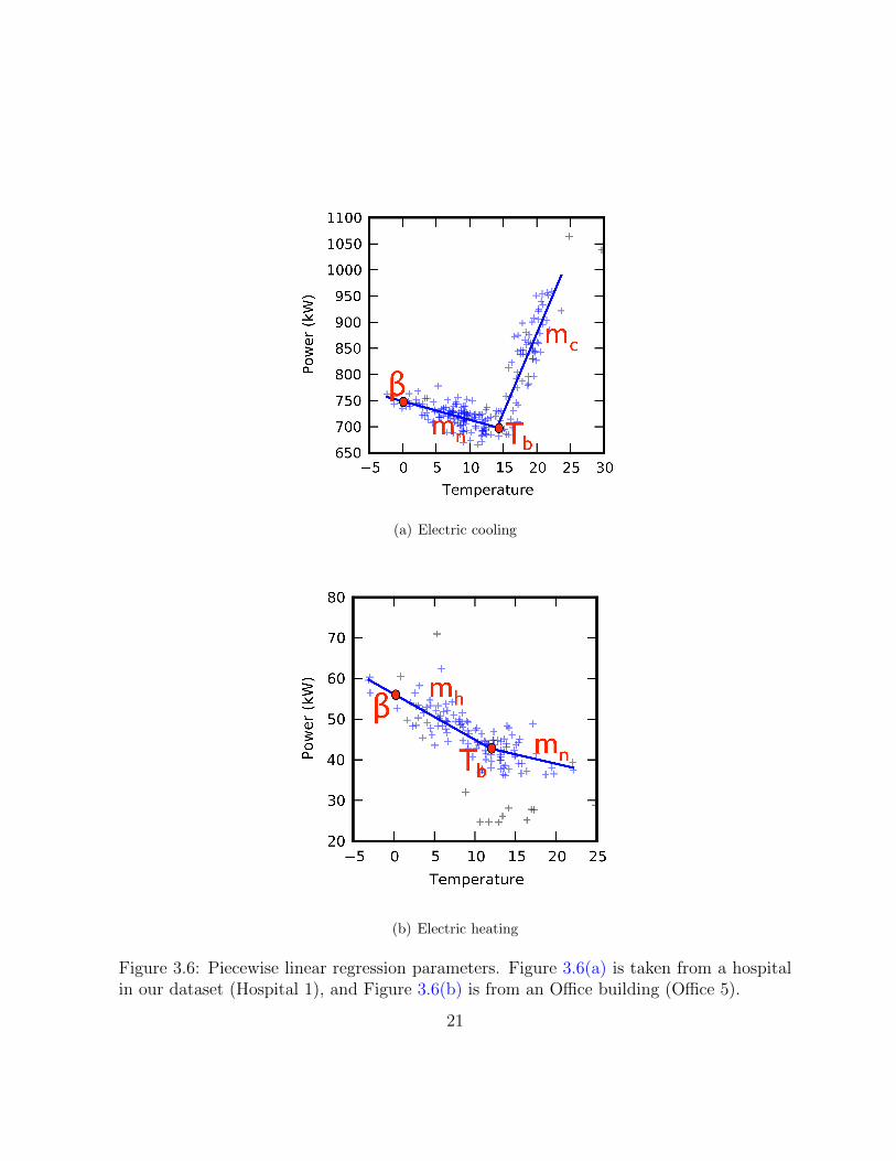
If DBSCAN identifies multiple clusters, Enerlytic chooses the cluster with the greatestnumber of points, and labels any other clusters as outliers. If any points are labelled as out-liers, Enerlytic discards these data and provides a notification. Following outlier detection,Enerlytic fits a piecewise linear regression model to each energy signature. Figures 3.6(a)and 3.6(b) show examples of buildings with electric cooling and heating piecewise linearregression parameters, respectively. The regression parameters are tabulated in Table 3.1,and the piecewise linear regressions are defined in Equations 3.1 and 3.2 for heating andcooling, respectively.

20

(a) Electric cooling

(b) Electric heating

Figure 3.6: Piecewise linear regression parameters. Figure 3.6(a) is taken from a hospitalin our dataset (Hospital 1), and Figure 3.6(b) is from an Office building (Office 5).

21

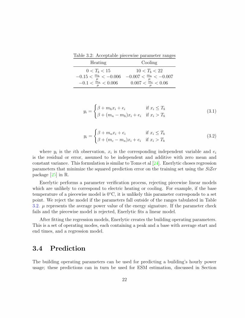
Table 3.2: Acceptable piecewise parameter ranges

Heating Cooling

0 < Tb < 15 10 < Tb < 22−0.15 < mh

µ< −0.006 −0.007 < mn

µ< −0.007

−0.1 < mn

µ< 0.006 0.007 < mc

µ< 0.06

yi =

{β +mhxi + ei if xi ≤ Tb

β + (mn −mh)xi + ei if xi > Tb(3.1)

yi =

{β +mnxi + ei if xi ≤ Tb

β + (mc −mn)xi + ei if xi > Tb(3.2)

where yi is the ith observation, xi is the corresponding independent variable and eiis the residual or error, assumed to be independent and additive with zero mean andconstant variance. This formulation is similar to Toms et al [24]. Enerlytic choses regressionparameters that minimize the squared prediction error on the training set using the SiZerpackage [25] in R.

Enerlytic performs a parameter verification process, rejecting piecewise linear modelswhich are unlikely to correspond to electric heating or cooling. For example, if the basetemperature of a piecewise model is 0◦C, it is unlikely this parameter corresponds to a setpoint. We reject the model if the parameters fall outside of the ranges tabulated in Table3.2. µ represents the average power value of the energy signature. If the parameter checkfails and the piecewise model is rejected, Enerlytic fits a linear model.

After fitting the regression models, Enerlytic creates the building operating parameters.This is a set of operating modes, each containing a peak and a base with average start andend times, and a regression model.

3.4 Prediction

The building operating parameters can be used for predicting a building’s hourly powerusage; these predictions can in turn be used for ESM estimation, discussed in Section

22

Prediction Dates

Outdoor Temperature

Operating Parameters

For eachDay

Find Matching Operating Mode

Evaluate Regression Model

Hourly Power

Figure 3.7: Prediction overview.

23

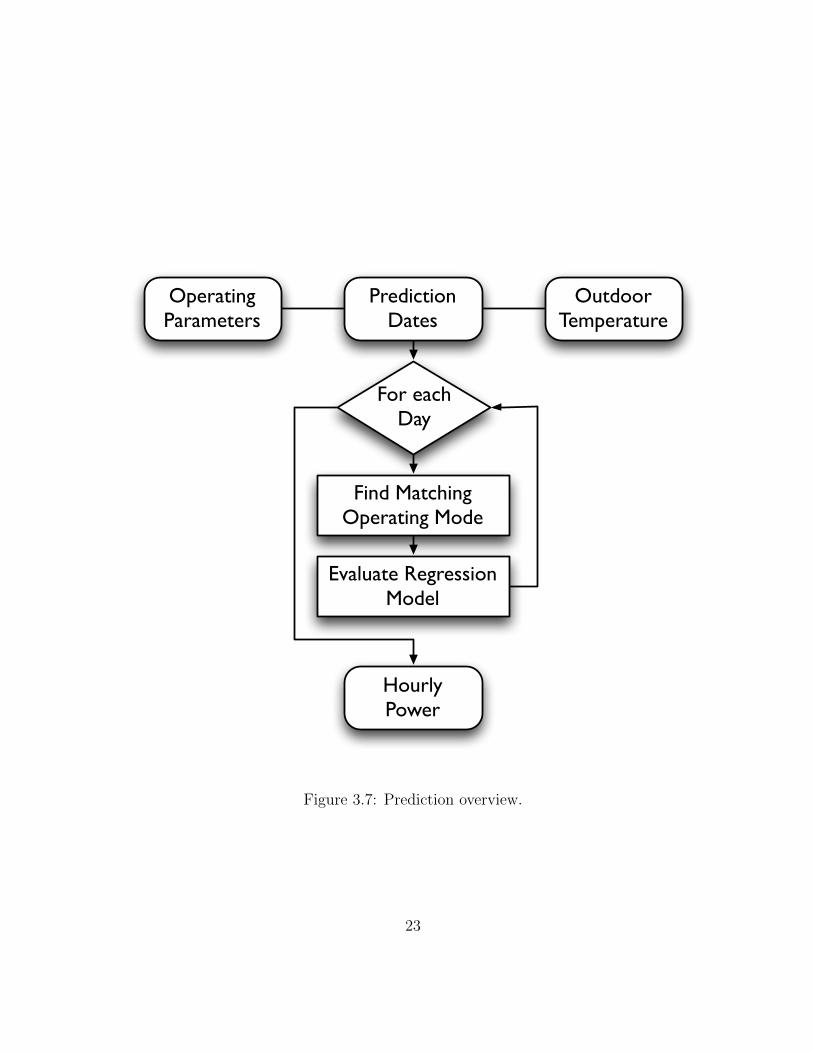
3.5, for validating the building operating parameters themselves, for forecasting electricalpower demand, or creating baseline models to evaluate the effectiveness of an ESM. Anoverview of the prediction process can be seen in Figure 3.7.

The prediction mechanism takes as input:

1. The building operating parameters

2. A list of dates for which we would like to generate predictions, referred to as theprediction dates

3. The hourly temperatures for the prediction dates

The prediction algorithm generates a prediction for each prediction date, and later concate-nates the results. It uses the labeller to determine the operating mode of each predictiondate, and retrieves the operating parameters corresponding to that operating mode. Thepeak and base regression models are then evaluated using the temperature input. Oncethe prediction algorithm has predicted the peak and base power value for each day, itre-creates each daily load profile by filling the peak and base periods with the predictedpeak and base values, respectively, and linearly interpolating during the ramping periods.

3.5 ESM Estimation

The building operating parameters can be used to estimate energy savings; this is doneby changing the building operating parameters. The energy savings estimates do notcorrespond to savings from a particular action or ESM. Instead, the savings correspondto a category of possible ESMs, which we call ESM scenarios. This provides a buildingoperator or an energy expert with the ability to estimate the potential energy savings dueto a change in energy consumption patterns. Relating the changes in the building operatingparameters to the building’s equipment and operation requires a deep knowledge of howa specific building is run. The building operator or energy expert must generate a listof building-specific actions or ESMs which will accompany the ESM scenario. Estimatesare obtained by substracting the predicted usage obtained using learned model parametersfrom the predicted usage under the modified model parameters. We demonstrate five ESMscenarios:

1. Peak or base average power reduction

24

2. Peak or base period reduction

3. Change of base temperature

4. Change of cooling or heating gradient

5. Change of operating mode

Figures 3.8 and 3.9 illustrate ESM scenarios 1-4, assuming a fixed cost of electricity of$0.05 per kWh. The first two ESM scenarios result from changing the parameters of thedaily load profile. For each predicted daily profile, we reduce the average peak by 10%, ordecreasing the length of the peak period by one hour. An overview of the ESM estimationprocess can be seen in Figure 3.10.

Scenarios three and four arise from changing the parameters of the regression models.Here, we adjust any piecewise linear regressions according to the ESM scenario: for exampleincreasing, the cooling base temperature by 1◦C, or by reducing the cooling gradient by10%. The final what-if scenario arises from creating a new labeller and changing thepredicted operating mode of the building. For example, assuming we have data to supportthe ESM scenario, we could estimate the difference in energy consumption if: a) a retrofithad not taken place, for example to verify energy savings; b) an anomalous event had notoccurred, such as equipment malfunctioning or being left on; or c) a low-power period,such as a holiday period, was extended.

3.6 Concluding Remarks

In this chapter we developed an algorithm, Enerlytic, which takes as input hourly powerconsumption, temperature data, and an optional labeller containing information aboutthe building’s operating modes, and creates a set of building operating parameters. Wedemonstrated how a building’s operating parameters can be used for prediction and toestimate energy savings. We believe there are many ways to extend this model, and wecontinue this discussion in Chapter 5, after presenting the model validation in Chapter 4.

25

Nov '0

9Dec

'09

Jan

'10 Fe

b '1

0M

ar '1

0Apr

'10

May

'10

Jun

'10 Ju

l '10 Aug '1

0Se

p '1

0 Oct '1

0Nov

'10

Dec '1

0Ja

n '1

1 Feb

'11

Mar

'11

Apr '1

1M

ay '1

1Ju

n '1

1 Jul '

11 Aug '1

1Se

p '1

1 Oct '1

1Nov

'11

Dec '1

1Ja

n '1

2 Feb

'12

0

10

00

0

20

00

0

30

00

0

40

00

0

50

00

0

60

00

0

70

00

0Monthly Energy Savings (kWh)

Month

ly S

avin

gs

for

Off

ice 1

050

0

10

00

15

00

20

00

25

00

30

00

35

00

40

00

45

00

Monthly Cost Savings ($)

10%

Peak

Reduct

ion

10%

Base

Reduct

ion

1h P

eak

Peri

od R

educt

ion

10%

Coolin

g G

radie

nt

Reduct

ion

1 D

eg. C

oolin

g B

ase

Tem

p Incr

ease

Fig

ure

3.8:

ESM

esti

mat

ion

for

anoffi

cebuildin

g.

26

Nov '0

9Dec

'09

Jan

'10 Fe

b '1

0M

ar '1

0Apr

'10

May

'10

Jun

'10 Ju

l '10 Aug '1

0Se

p '1

0 Oct '1

0Nov

'10

Dec '1

0Ja

n '1

1 Feb

'11

Mar

'11

Apr '1

1M

ay '1

1Ju

n '1

1 Jul '

11 Aug '1

1Se

p '1

1 Oct '1

1Nov

'11

Dec '1

1Ja

n '1

2 Feb

'12

0

50

00

10

00

0

15

00

0

20

00

0

25

00

0

30

00

0

35

00

0Monthly Energy Savings (kWh)

Month

ly S

avin

gs

for

Hosp

ital 1

050

0

10

00

15

00

20

00

25

00

Monthly Cost Savings ($)

10%

Peak

Reduct

ion

10%

Base

Reduct

ion

1h P

eak

Peri

od R

educt

ion

10%

Coolin

g G

radie

nt

Reduct

ion

1 D

eg. C

oolin

g B

ase

Tem

p Incr

ease

Fig

ure

3.9:

ESM

esti

mat

ion

for

ahos

pit

al.

27

Modify Operating Parameters

Create ESM Prediction

Create Baseline Prediction

Calc monthly energy, cost savings

OperatingParameters

ESMPrediction

Data

Figure 3.10: ESM estimation overview.

28

Chapter 4

Evaluation

We evaluate the building operating parameters by testing the prediction algorithm on adataset provided by Pulse Energy, a leading Energy Information System (EIS) provider [26].The dataset contains:

• Two schools, two hospitals, one grocery store and five office buildings

• Buildings in Western and Eastern Canada, and North-Western and South-EasternUnited States.

• An average of over two years of data per building for a total of over 21 years of meterdata

• Hourly average power consumption and accompanying hourly outdoor temperaturedata

Table A.1 contains a more detailed description of the dataset. We use buildings thatspan a variety of commercial areas and geographies and use several years of data for eachbuilding to evaluate Enerlytic under a range of seasons, climatic zones, and electricaldemand patterns.

We measure the accuracy of our predictions using K=4 fold cross validation on eachbuilding. The partitions for each fold are chosen at random. The default labeller is usedto label and partition the data for each building into weekdays and weekends. We measureprediction accuracy using the coefficient-of-variation of the root-mean-squared-error (CV-RMSE) and mean-bias-error (MBE); these are standard metrics in the building energyprediction literature [14] [9] [13]. We benchmark our prediction algorithm against a state-of-the-art prediction algorithm that uses kernel regression [9].

29

4.1 Results

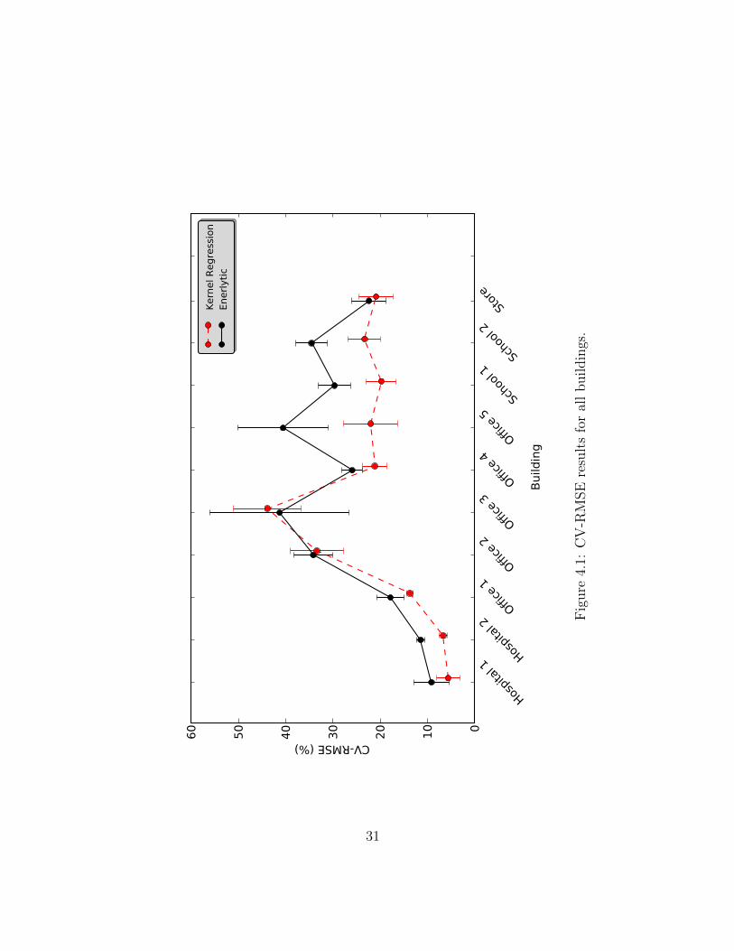
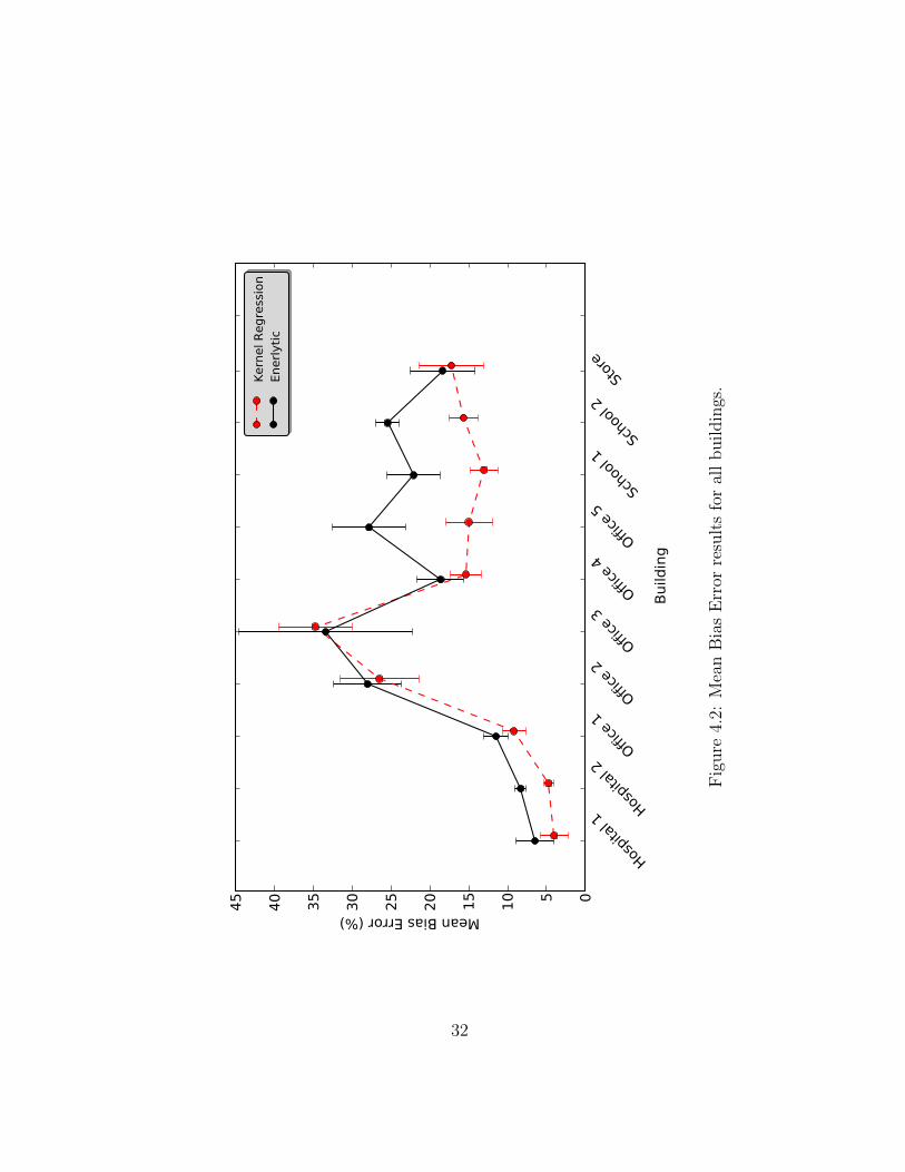
Figures 4.1 and 4.2 show, respectively, a summary of the CV-RMSE and MBE perfor-mance of our method (“Enerlytic”) and the benchmark (“Kernel Regression”). The 90%confidence intervals represent the contributions from each of the four folds.

Enerlytic is less accurate at prediction than the benchmark; this is to be expecteddue to the relative simplicity and restrictive parameterization of the building operatingparameters, and because the primary goal of the building operating parameters is to gaininsight and be used as input to other systems, not solely to create an accurate predictionalgorithm. We believe the prediction error is comparable enough to current practice toenable the building operating parameters to be used for prediction, and also as input toother systems such as ESM estimation and benchmarking.

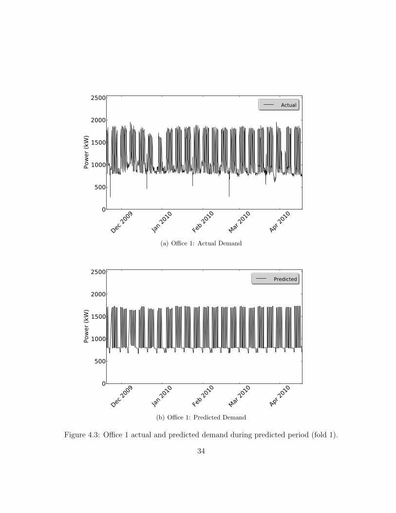
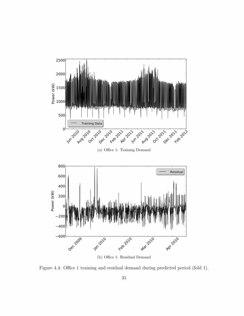
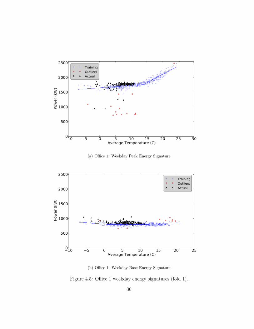
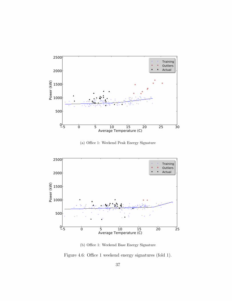
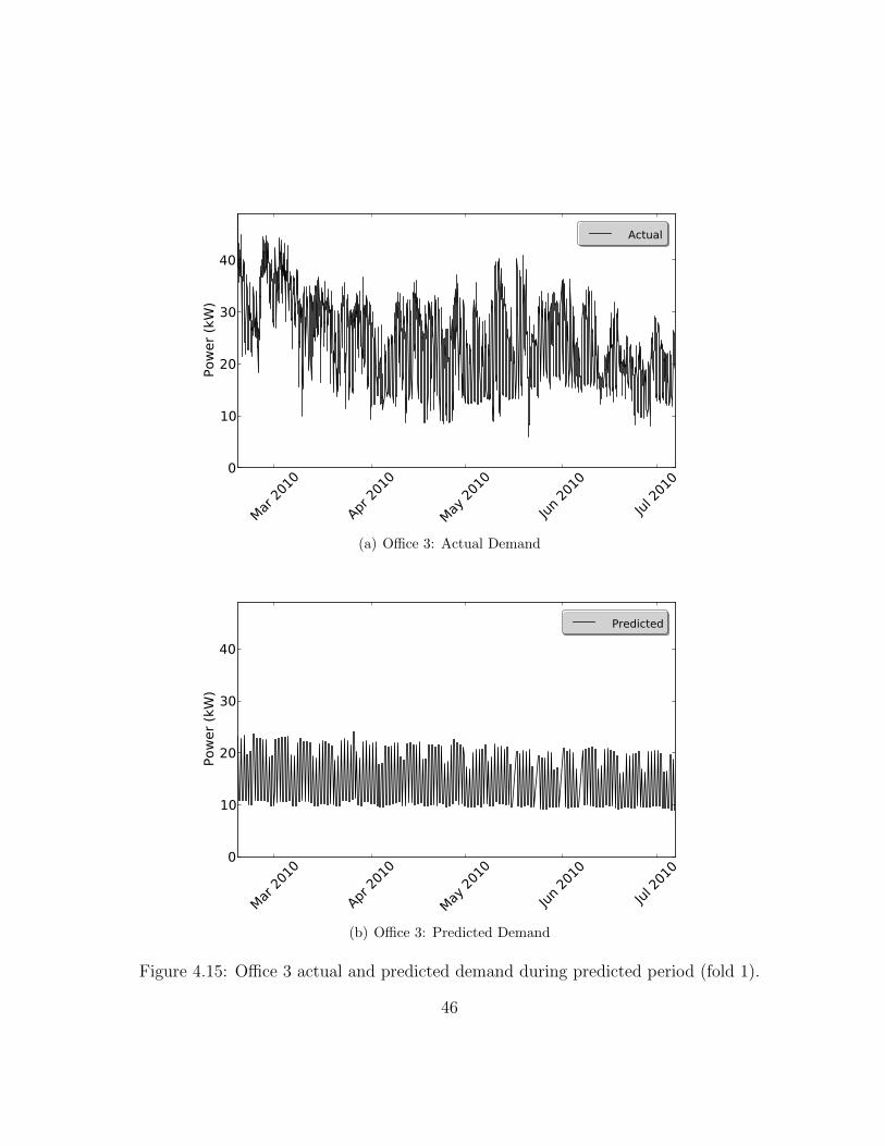
The results shown in Figures 4.1 and 4.2 fall into two categories: buildings where thedefault labeller identifies the building’s operating modes, and buildings where the defaultlabeller misses significant operating modes of a building. When a building primarily hasweekend and weekday operating modes (Hospitals 1, 2; Offices 1, 2, 4; Store), the predictionperformance of their building operating parameters is quite similar to the benchmark. Anexample of this can be seen in the detailed results of Office 1, shown in Figures 4.3-4.6.Figure 4.3 shows the actual and predicted demand during the prediction period, Figure4.4 shows the prediction error (residual) and the data used to create (train) the buildingoperating parameters. Figures 4.5 and 4.6 show the energy signatures for the weekday andweekend operating modes, respectively. Statutory holidays are a primary source of error,as seen in Figure 4.4(b) where holidays appear as spikes in the residual, and in Figure4.5(a), where holidays are classified as outliers. Creating a labeller that labels statuatoryholidays may further improve prediction performance.

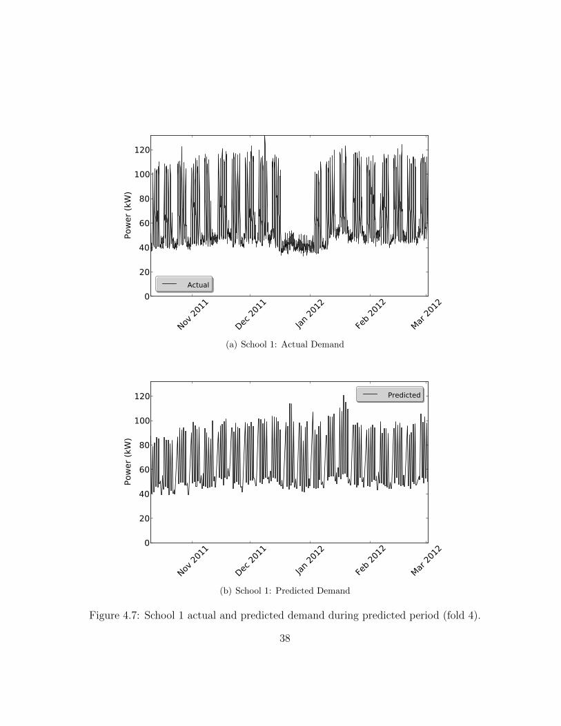
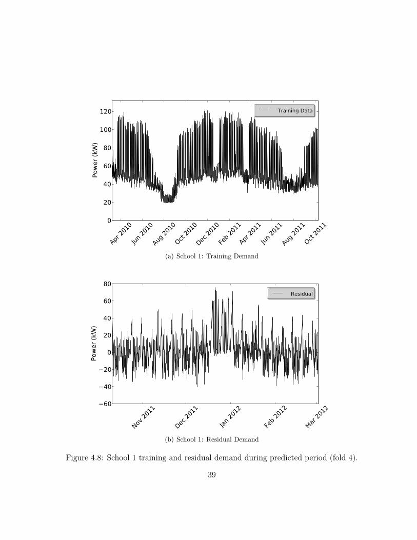
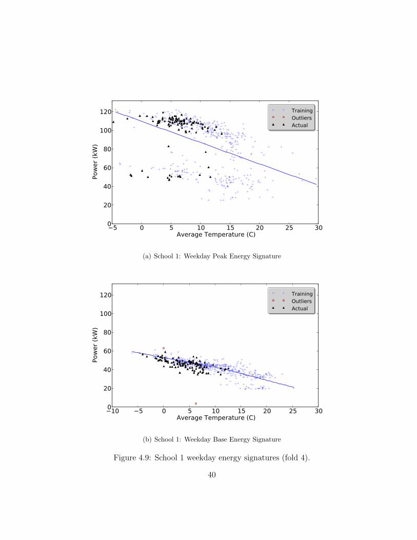
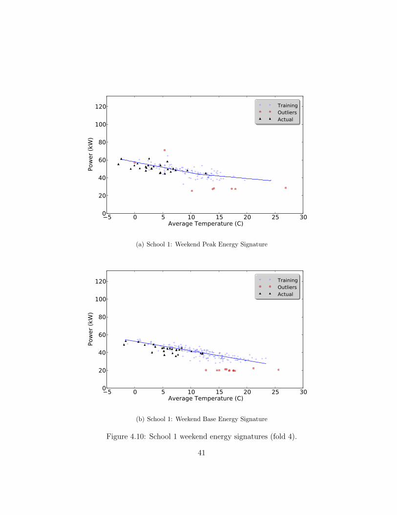
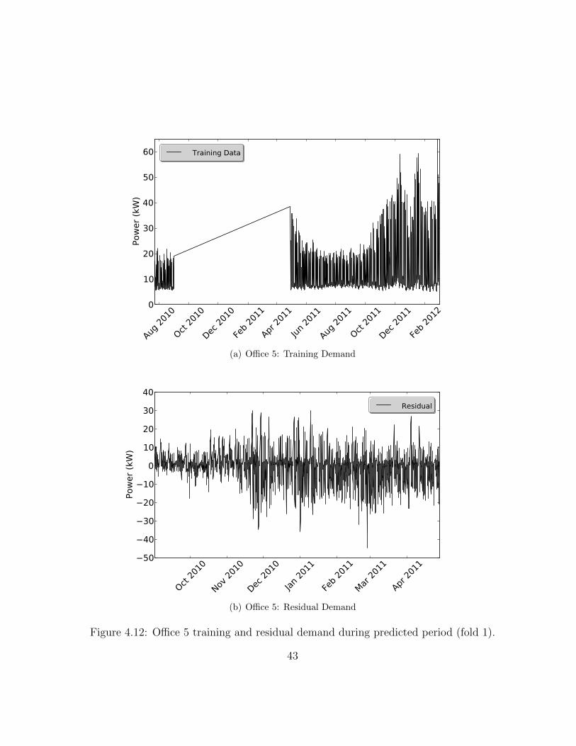
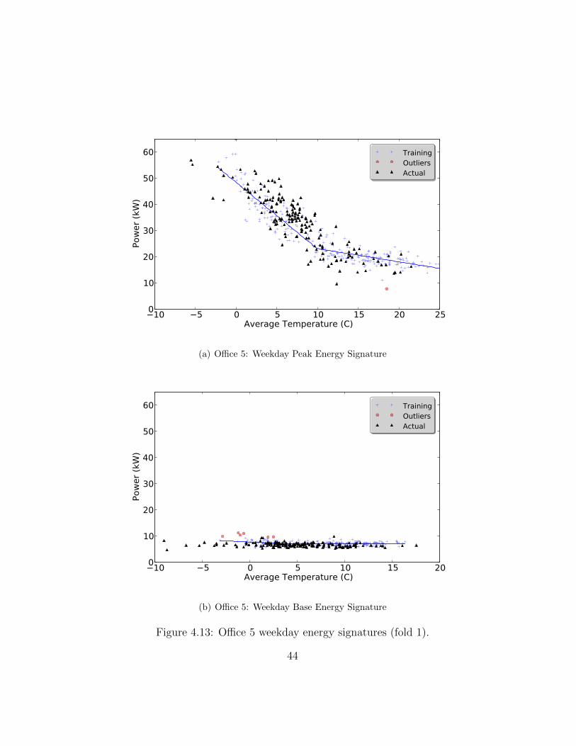
The remaining buildings (Schools 1, 2; Offices 3, 5) have significant operating modesthat were not identified by the default labeller. The schools had summer holiday periodsthat caused poor regression fits due to Simpson’s paradox [22]; an example of this can beseen in Figures 4.7-4.10. Outlier detection was not effective. An improved outlier detec-tion strategy may improve prediction performance, but we suggest future work investigatedefault labellers that create labels based on the underlying statistics of the data. Figures4.11-4.14 show an example of the prediction performance for Office 5. Figure 4.13(a) showsthere are shifts in the consumption patterns of the building’s electric heating system; thereare small translations between the “training” and “actual” data, causing a systemic biasin prediction error. These changes in the building’s electric heating system can be inter-preted as a change in operating mode. This could be captured by labelling the building

30

Hospi

tal 1

Hospi

tal 2

Office

1Offi

ce 2

Office

3Offi

ce 4

Office

5Sc

hool

1Sc

hool

2

Stor

e

Build

ing

0

10

20

30

40

50

60

CV-RMSE (%)K

ern

el R

egre

ssio

nEnerl

yti

c

Fig

ure

4.1:

CV

-RM

SE

resu

lts

for

all

buildin

gs.

31

Hospi

tal 1

Hospi

tal 2

Office

1Offi

ce 2

Office

3Offi

ce 4

Office

5Sc

hool

1Sc

hool

2

Stor

e

Build

ing

05

10

15

20

25

30

35

40

45

Mean Bias Error (%)K

ern

el R

egre

ssio

nEnerl

yti

c

Fig

ure

4.2:

Mea

nB

ias

Err

orre

sult

sfo

ral

lbuildin

gs.

32

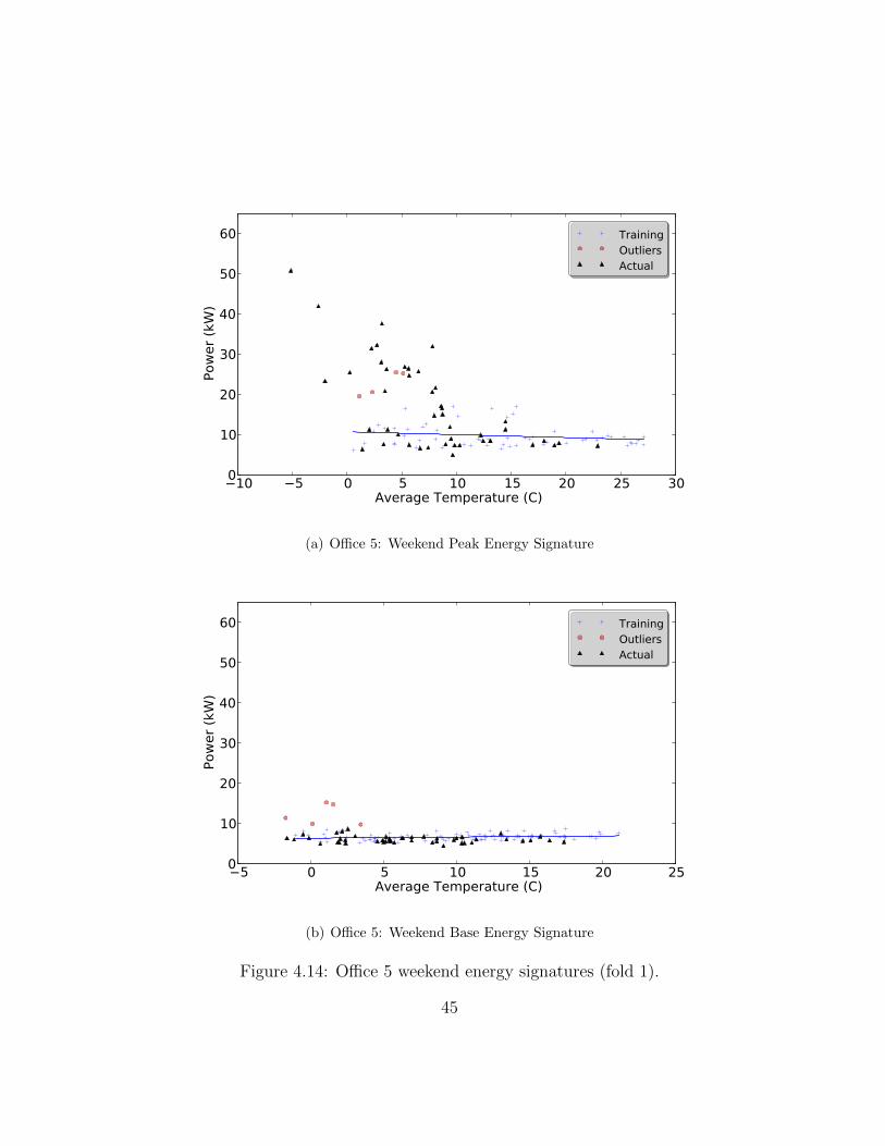
as being in different operating modes during these two periods. This result also showsthe building operating parameters generalize poorly compared to the benchmark. Anotherexample of poor generalization (overfitting) can been seen in Figure 4.14(a), where thebuilding operating parameters do not anticipate the use of electric heating on weekends.Future work may improve the model’s ability to generalize by considering the underlyingdistribution of the data: if the variance is sufficiently high, a stochastic process could beused for prediction instead of linear regressions.

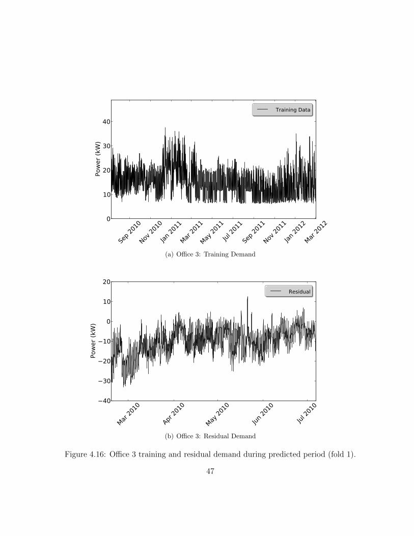
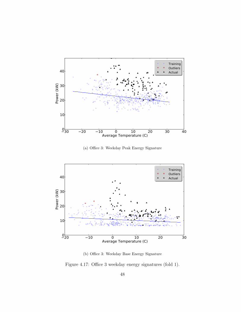
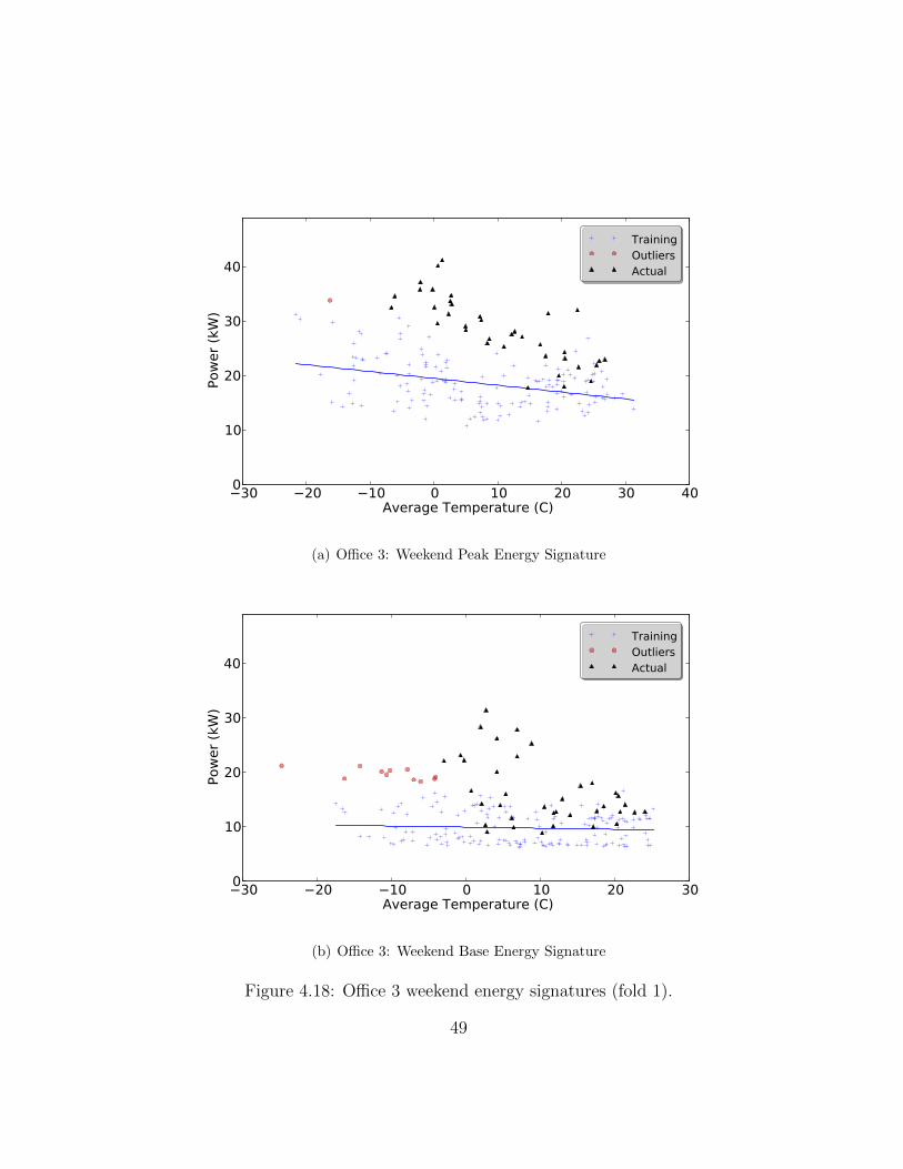
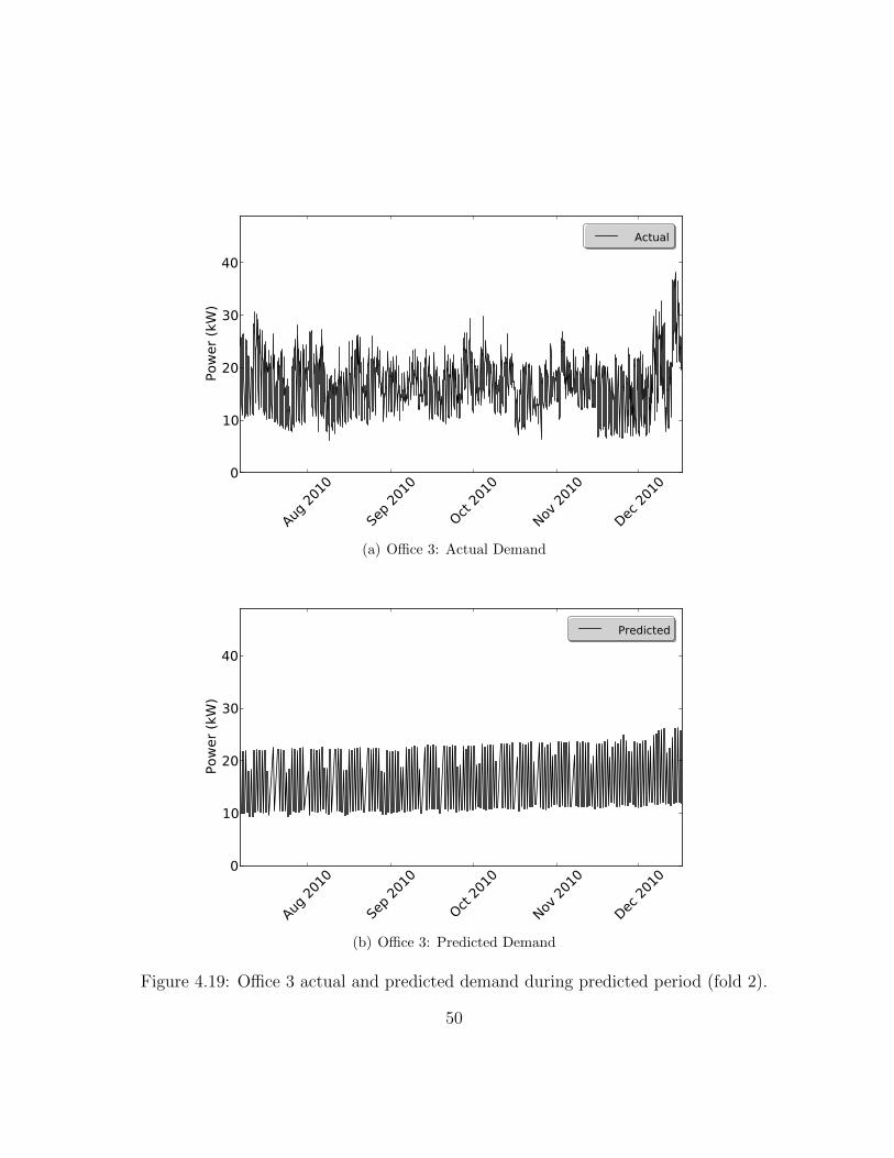
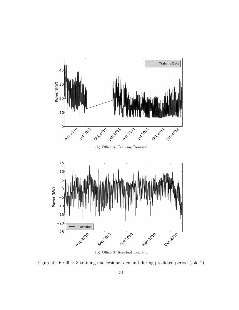
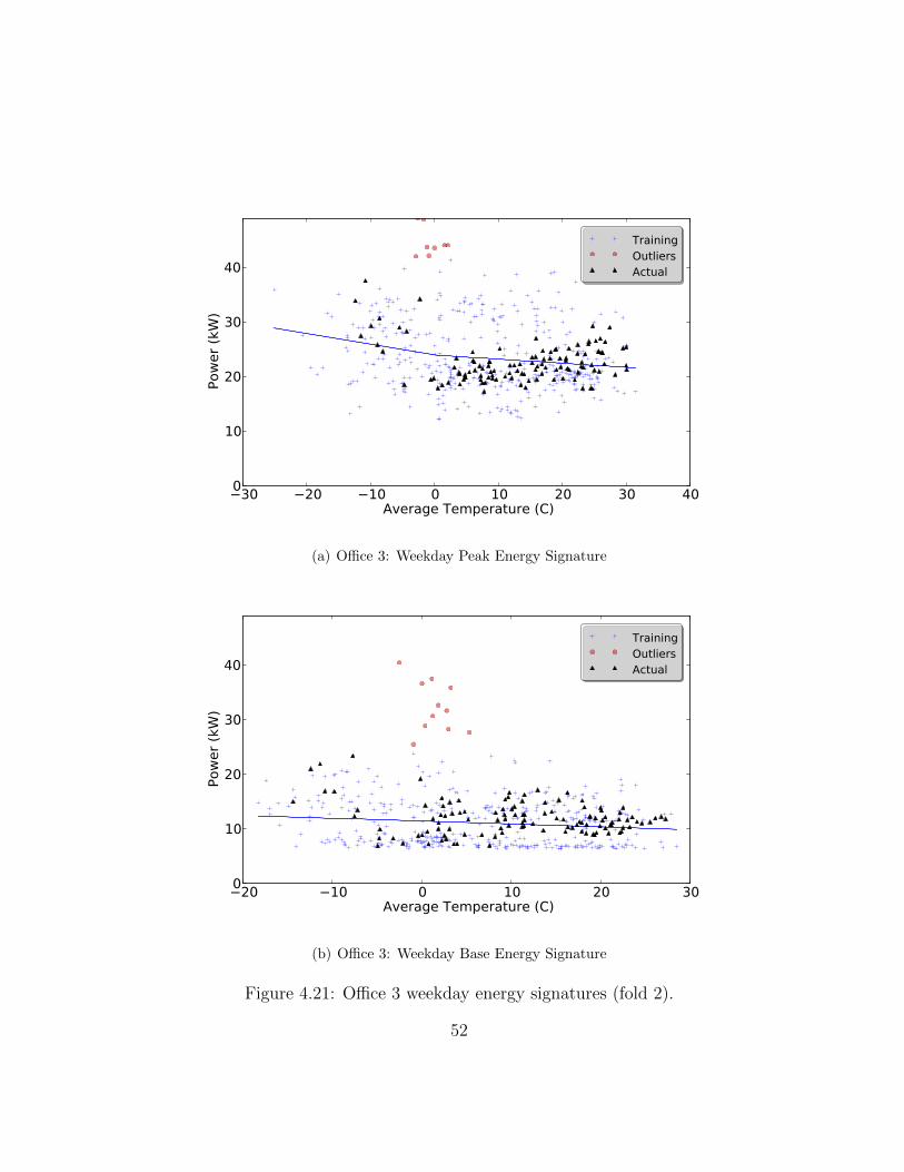
Office 3 had gradual changes in the load profile throughout its measurement period;this can be seen by comparing Figure 4.15(a), which shows the data in the first fold,to Figure 4.16(a), which shows the data in the final three folds. Figures 4.15-4.18 showdetailed prediction performance for the first fold of Office 3. Figure 4.15(a) shows Office3 initially had relatively high electric energy consumption; Figure 4.16(a) indicates thisconsumption level fell and remained relatively low during the rest of the measurementperiod. When the data from Figure 4.16(a) was used to predict the period shown in Figure4.15(a), the prediction error was high since the training data was not representative ofthe demand during the prediction period—the building was in a different operating mode.When predicting folds 2, 3, and 4, the high consumption period fell in the training periodinstead of the prediction period; the outlier detection mechanism typically labelled thehigh consumption days as outliers. Figures 4.19-4.22 show the prediction performance ofthe second fold of Office 3. As seen in Figures 4.21 and 4.22, data in the high consumptionperiod were labelled as outliers. The transient period of high consumption, combinedwith the outlier detection, led to relatively low prediction error for folds 2, 3, and 4,while the error from fold 1 remained high. This caused a large variation in predictionperformance for this building, despite the mean prediction performance being comparableto the benchmark. Like Office 5, prediction performance may be improved by partitioningthe dataset into different operating modes using a more advanced labelling scheme, or byusing a regression model that is less prone to overfitting.

In summary, Enerlytic predicts well when the operating modes in the training data andprediction period have been identified. The non-linear kernel regression generalizes moreeffectively than the piecewise linear models, particularly when operating modes are notidentified by the labeller. Future work could address these limitations by creating moreadvanced labellers and by investigating regression methods that are able to both provideinsight and also avoid overfitting.

33

Dec 2

009

Jan

2010

Feb

2010

Mar

201

0

Apr 2

010

0

500

1000

1500

2000

2500

Pow

er

(kW

)

Actual

(a) Office 1: Actual Demand

Dec 2

009

Jan

2010

Feb

2010

Mar

201

0

Apr 2

010

0

500

1000

1500

2000

2500

Pow

er

(kW

)

Predicted

(b) Office 1: Predicted Demand

Figure 4.3: Office 1 actual and predicted demand during predicted period (fold 1).

34

Jun

2010

Aug 2

010

Oct 2

010

Dec 2

010

Feb

2011

Apr 2

011

Jun

2011

Aug 2

011

Oct 2

011

Dec 2

011

Feb

2012

0

500

1000

1500

2000

2500

Pow

er

(kW

)

Training Data

(a) Office 1: Training Demand

Dec 2

009

Jan

2010

Feb

2010

Mar

201

0

Apr 2

010

600

400

200

0

200

400

600

800

Pow

er

(kW

)

Residual

(b) Office 1: Residual Demand

Figure 4.4: Office 1 training and residual demand during predicted period (fold 1).

35

10 5 0 5 10 15 20 25 30Average Temperature (C)

0

500

1000

1500

2000

2500

Pow

er

(kW

)

TrainingOutliersActual

(a) Office 1: Weekday Peak Energy Signature

10 5 0 5 10 15 20 25Average Temperature (C)

0

500

1000

1500

2000

2500

Pow

er

(kW

)


(b) Office 1: Weekday Base Energy Signature

Figure 4.5: Office 1 weekday energy signatures (fold 1).

36


0

500

1000

1500

2000

2500

Pow

er

(kW

)


(a) Office 1: Weekend Peak Energy Signature

5 0 5 10 15 20 25Average Temperature (C)

0

500

1000

1500

2000

2500

Pow

er

(kW

)


(b) Office 1: Weekend Base Energy Signature

Figure 4.6: Office 1 weekend energy signatures (fold 1).

37

Nov 2

011

Dec 2

011

Jan

2012

Feb

2012

Mar

201

20

20

40

60

80

100

120

Pow

er

(kW

)

Actual

(a) School 1: Actual Demand

Nov 2

011

Dec 2

011

Jan

2012

Feb

2012

Mar

201

20

20

40

60

80

100

120

Pow

er

(kW

)

Predicted

(b) School 1: Predicted Demand

Figure 4.7: School 1 actual and predicted demand during predicted period (fold 4).

38

Apr 2

010

Jun

2010

Aug 2

010

Oct 2

010

Dec 2

010

Feb

2011

Apr 2

011

Jun

2011

Aug 2

011

Oct 2

011

0

20

40

60

80

100

120

Pow

er

(kW

)

Training Data

(a) School 1: Training Demand

Nov 2

011

Dec 2

011

Jan

2012

Feb

2012

Mar

201

260

40

20

0

20

40

60

80

Pow

er

(kW

)

Residual

(b) School 1: Residual Demand

Figure 4.8: School 1 training and residual demand during predicted period (fold 4).

39


0

20

40

60

80

100

120

Pow

er

(kW

)


(a) School 1: Weekday Peak Energy Signature


0

20

40

60

80

100

120

Pow

er

(kW

)


(b) School 1: Weekday Base Energy Signature

Figure 4.9: School 1 weekday energy signatures (fold 4).

40


0

20

40

60

80

100

120

Pow

er

(kW

)


(a) School 1: Weekend Peak Energy Signature


0

20

40

60

80

100

120

Pow

er

(kW

)


(b) School 1: Weekend Base Energy Signature

Figure 4.10: School 1 weekend energy signatures (fold 4).

41

Oct 2

010

Nov 2

010

Dec 2

010

Jan

2011

Feb

2011

Mar

201

1

Apr 2

011

0

10

20

30

40

50

60

Pow

er

(kW

)

Actual


Oct 2

010

Nov 2

010

Dec 2

010

Jan

2011

Feb

2011

Mar

201

1

Apr 2

011

0

10

20

30

40

50

60

Pow

er

(kW

)

Predicted



42

Aug 2

010

Oct 2

010

Dec 2

010

Feb

2011

Apr 2

011

Jun

2011

Aug 2

011

Oct 2

011

Dec 2

011

Feb

2012

0

10

20

30

40

50

60

Pow

er

(kW

)

Training Data


Oct 2

010

Nov 2

010

Dec 2

010

Jan

2011

Feb

2011

Mar

201

1

Apr 2

011

50

40

30

20

10

0

10

20

30

40

Pow

er

(kW

)

Residual



43


0

10

20

30

40

50

60

Pow

er

(kW

)




0

10

20

30

40

50

60

Pow

er

(kW

)




44


0

10

20

30

40

50

60

Pow

er

(kW

)




0

10

20

30

40

50

60

Pow

er

(kW

)




45

Mar

201

0

Apr 2

010

May

201

0

Jun

2010

Jul 2

010

0

10

20

30

40

Pow

er

(kW

)

Actual


Mar

201

0

Apr 2

010

May

201

0

Jun

2010

Jul 2

010

0

10

20

30

40

Pow

er

(kW

)

Predicted



46

Sep

2010

Nov 2

010

Jan

2011

Mar

201

1

May

201

1

Jul 2

011

Sep

2011

Nov 2

011

Jan

2012

Mar

201

20

10

20

30

40

Pow

er

(kW

)

Training Data


Mar

201

0

Apr 2

010

May

201

0

Jun

2010

Jul 2

010

40

30

20

10

0

10

20

Pow

er

(kW

)

Residual



47


0

10

20

30

40

Pow

er

(kW

)



20 10 0 10 20 30Average Temperature (C)

0

10

20

30

40

Pow

er

(kW

)




48


0

10

20

30

40

Pow

er

(kW

)




0

10

20

30

40

Pow

er

(kW

)




49

Aug 2

010

Sep

2010

Oct 2

010

Nov 2

010

Dec 2

010

0

10

20

30

40

Pow

er

(kW

)

Actual


Aug 2

010

Sep

2010

Oct 2

010

Nov 2

010

Dec 2

010

0

10

20

30

40

Pow

er

(kW

)

Predicted



50

Apr 2

010

Jul 2

010

Oct 2

010

Jan

2011

Apr 2

011

Jul 2

011

Oct 2

011

Jan

2012

0

10

20

30

40

Pow

er

(kW

)

Training Data


Aug 2

010

Sep

2010

Oct 2

010

Nov 2

010

Dec 2

010

25

20

15

10

5

0

5

10

15

Pow

er

(kW

)

Residual



51


0

10

20

30

40

Pow

er

(kW

)



20 10 0 10 20 30Average Temperature (C)

0

10

20

30

40

Pow

er

(kW

)




52


0

10

20

30

40

Pow

er

(kW

)




0

10

20

30

40

Pow

er

(kW

)




53

Chapter 5

Implementation

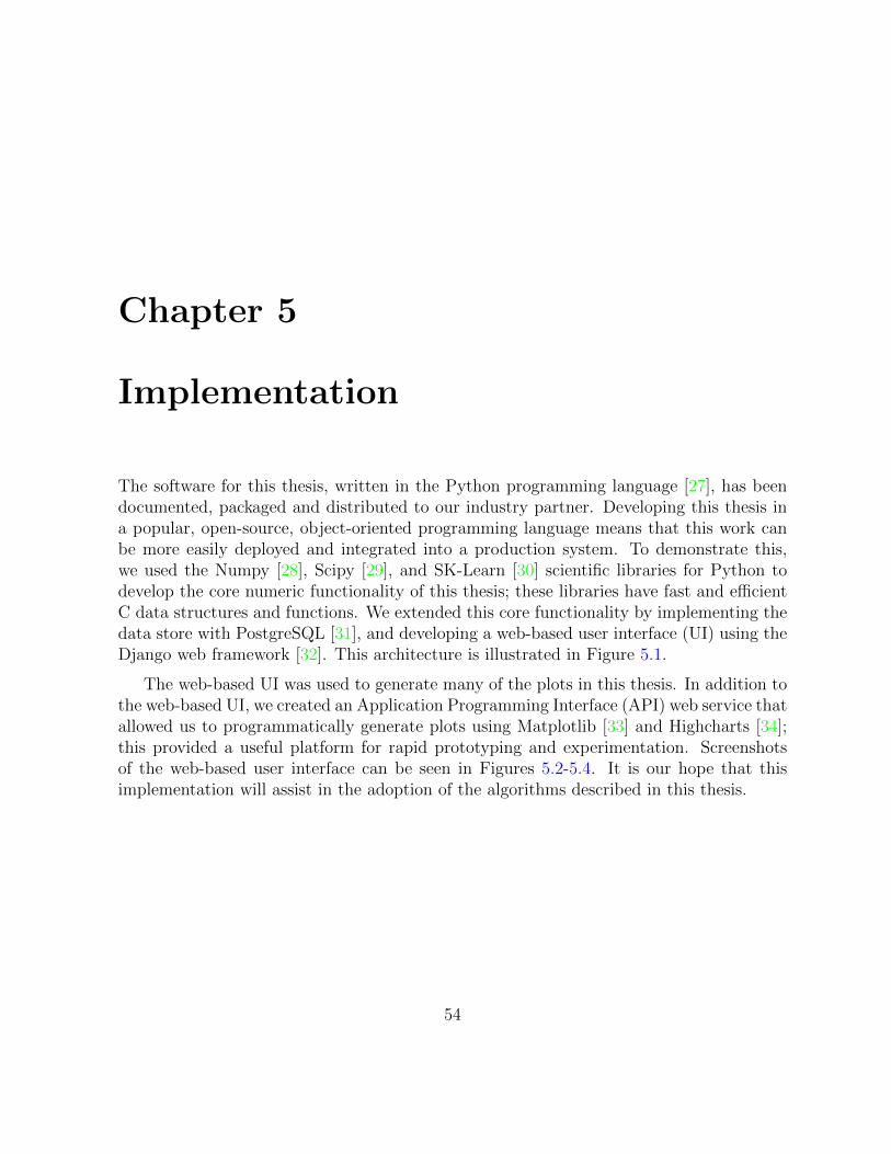
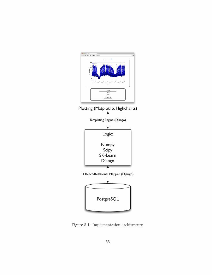
The software for this thesis, written in the Python programming language [27], has beendocumented, packaged and distributed to our industry partner. Developing this thesis ina popular, open-source, object-oriented programming language means that this work canbe more easily deployed and integrated into a production system. To demonstrate this,we used the Numpy [28], Scipy [29], and SK-Learn [30] scientific libraries for Python todevelop the core numeric functionality of this thesis; these libraries have fast and efficientC data structures and functions. We extended this core functionality by implementing thedata store with PostgreSQL [31], and developing a web-based user interface (UI) using theDjango web framework [32]. This architecture is illustrated in Figure 5.1.

The web-based UI was used to generate many of the plots in this thesis. In addition tothe web-based UI, we created an Application Programming Interface (API) web service thatallowed us to programmatically generate plots using Matplotlib [33] and Highcharts [34];this provided a useful platform for rapid prototyping and experimentation. Screenshotsof the web-based user interface can be seen in Figures 5.2-5.4. It is our hope that thisimplementation will assist in the adoption of the algorithms described in this thesis.

54

Plotting (Matplotlib, Highcharts)

Logic:

NumpyScipy

SK-LearnDjango

PostgreSQL

Templating Engine (Django)

Object-Relational Mapper (Django)

Figure 5.1: Implementation architecture.

55

Fig

ure

5.2:

Web

-bas

eduse

rin

terf

ace:

Hom

epag

e.

56

Fig

ure

5.3:

Web

-bas

eduse

rin

terf

ace:

Plo

tse

lect

or.

57

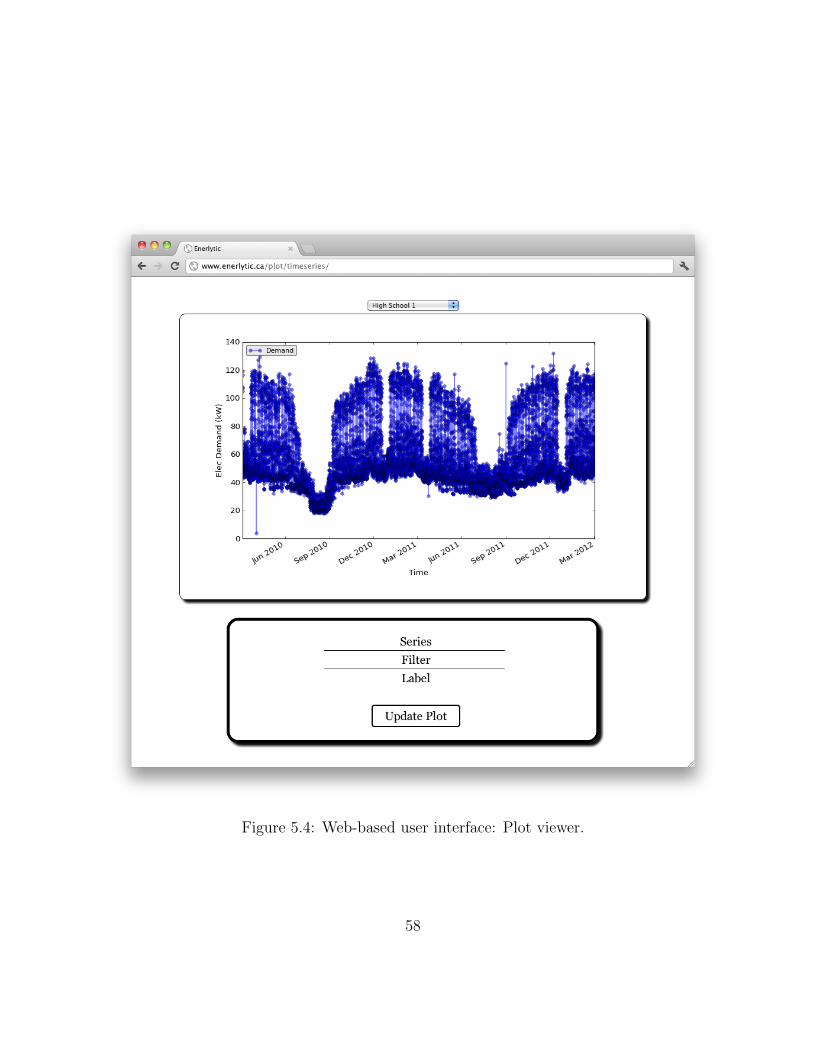
Figure 5.4: Web-based user interface: Plot viewer.

58

Chapter 6

Conclusion

This thesis describes the development, implementation, and evaluation of Enerlytic, analgorithm that takes as input electrical meter data from a commercial building and outputsits operating parameters. These operating parameters can be used by an energy expertto rapidly assess the building’s energy consumption patterns without a time consumingand expensive site visit. Moreover, we have shown how these operating parameters can beused as input to other systems for prediction and estimating possible energy savings. Abuilding operator can use Enerlytic to determine potential cost savings from implementingenergy savings measures without engaging the services of an expensive energy expert.

Prior work includes the use of piecewise linear models for estimating energy savingsin buildings [16] [17], and partitioning the daily load profile for prediction [19] or demandresponse [18]. However, this work either uses daily averages of energy useage, or doesnot develop a model which can be manipulated to obtain energy savings estimates. Ourapproach takes into account the various operating modes of a building through labelling.It models the peak and base load as a function of outdoor air temperature using piecewiselinear regressions. The algorithmic creation of the building operating parameters enablesfuture work, such as benchmarking a portfolio of buildings, demand response, and novelvisualization methods, as discussed below.

We tested our approach on a dataset containing 10 buildings and 21 years of meterdata; we show that the building operating parameters offer comparable performance to ablack-box prediction method used in the industry [9]. This thesis is the product of a yearlong collaboration with Pulse Energy. The formulation of this problem is a direct result ofworking with the energy experts at Pulse Energy and from conversations with commercialbuilding operators. The software for this thesis has been documented, packaged, and

59

distributed to an industry partner. We hope that this thesis will allow energy experts andbuilding operators to easily realize financial and environmental benefit from the algorithmicanalysis of commercial meter data.

6.1 Limitations

There are several limitations to this thesis.

1. The prediction accuracy of the building operating parameters is comparable to thebenchmark model in the majority of buildings in our dataset; in some buildings,however, the prediction accuracy is significantly lower. We attribute this to poorregression fits. To address this, we suggest an iterative regression mechanism thatfits a set of regression models and considers the tradeoff between model complexityversus an error metric, such as the CV-RMSE prediction error. Models in this setcould include non-linear or bin-based [20] models.

2. We use only one benchmark for the accuracy of Enerlytic’s predictions; this bench-mark is not the most accurate prediction method available [9]. Future work couldconsider evaluating the prediction accuracy of the building operating parametersagainst other prediction models such as those described in references [14] [18] [19].

3. Our work considers only electrical energy; it is possible to apply Enerlytic to otherfuel sources, such as natural gas.

4. We have not verified that energy savings measures estimates lead to energy savingsin buildings. Future work could verify this with help from industry partners.

5. We introduce a mechanism for labelling the operating modes of a building, but testthe prediction accuracy using only the default labeller. We hope that future workwill create case studies evaluating the effect of labelling on both prediction accuracyand providing insight into energy consumption patterns.

6. Enerlytic uses a piecewise regression with a single change-point, so that it is applicableto buildings with either electric heating or cooling or neither. Future work caninvestigate buildings with both electric heating and cooling.

7. We have evaluated our work using only hourly meter data; we encourage future workto investigate the effects of different data resolutions.

60

6.2 Future Work

In addition to addressing the limitations of this thesis, we believe there are many op-portunities for extending our work. We would like to quantify the computational cost ofEnerlytic compared with other models such as Brown et al [9]. We suspect Enerlytic, dueto its relative simplicity, is considerably faster. If true, we believe this is a significantopportunity. If predictions can be generated on-the-fly, they do not need to be cached orpersisted; this greatly simplifies the implementation, maintenance and scalability of anyproduction system that uses Enerlytic. On-the-fly predictions may also lead to improveduser experience by allowing a user to interact with the building’s operating parameters inreal time.

We believe the building operating parameters can be used for many other applications.Several that are not explored in this thesis include: novel methods for visualization, suchas visualizing the average peak and base start times for an operating mode; evaluatingdemand-response opportunities using peak-load shifting; and benchmarking a portfolio ofbuildings. Future work should formalize the building operating parameters by specifyingan application programming interface (API).

61

References

[1] United States Energy Information Administration. Electric Power Annual 2011, Ta-ble ES1. http://www.eia.gov/electricity/annual/pdf/tablees1.pdf. Accessed:29/06/2012.

[2] Natural Resources Canada. Total End-Use Sector-Energy Use Analysis.http://oee.nrcan.gc.ca/corporate/statistics/neud/dpa/tablesanalysis2/

aaa_ca_1_e_4.cfm. Accessed: 29/06/2012.

[3] Natural Resources Canada. Total End-Use Sector-GHG Emissions. http:

//oee.nrcan.gc.ca/corporate/statistics/neud/dpa/tablesanalysis2/aaa_

00_1_e_4.cfm. Accessed: 29/06/2012.

[4] United States Energy Information Administration. Frequently Asked Questions: Howmany smart meters are installed in the U.S. and who has them? http://www.eia.

gov/tools/faqs/faq.cfm?id=108&t=3. Accessed: 29/06/2012.

[5] Ontario Independent Electricity System Operator. Smart Grid Forum Re-port, May 2011. http://www.ieso.ca/imoweb/pubs/smart_grid/Smart_Grid_

Forum-Report-May_2011.pdf. Accessed: 29/06/2012.

[6] B.C. Hydro. Continuous Optimization Success Stories: Jawl Proper-ties. http://www.bchydro.com/etc/medialib/internet/documents/power_

smart/success_stories/A11_530_success_story_Jawl.Par.0001.File.

A11-530-success-story-Jawl.pdf. Accessed: 29/06/2012.

[7] B.C. Hydro. Continuous Optimization Program. http://www.bchydro.com/

powersmart/business/commercial/continuous_optimization.html. Accessed:29/06/2012.

62

http://www.eia.gov/electricity/annual/pdf/tablees1.pdf

http://oee.nrcan.gc.ca/corporate/statistics/neud/dpa/tablesanalysis2/aaa_ca_1_e_4.cfm

http://oee.nrcan.gc.ca/corporate/statistics/neud/dpa/tablesanalysis2/aaa_ca_1_e_4.cfm

http://oee.nrcan.gc.ca/corporate/statistics/neud/dpa/tablesanalysis2/aaa_00_1_e_4.cfm



http://www.eia.gov/tools/faqs/faq.cfm?id=108&t=3

http://www.eia.gov/tools/faqs/faq.cfm?id=108&t=3

http://www.ieso.ca/imoweb/pubs/smart_grid/Smart_Grid_Forum-Report-May_2011.pdf

http://www.ieso.ca/imoweb/pubs/smart_grid/Smart_Grid_Forum-Report-May_2011.pdf

http://www.bchydro.com/etc/medialib/internet/documents/power_smart/success_stories/A11_530_success_story_Jawl.Par.0001.File.A11-530-success-story-Jawl.pdf



http://www.bchydro.com/powersmart/business/commercial/continuous_optimization.html

http://www.bchydro.com/powersmart/business/commercial/continuous_optimization.html

[8] B.C. Hydro. Continuous Optimization Program Services Funding for Commer-cial Buildings Agreement. http://www.bchydro.com/etc/medialib/internet/

documents/power_smart/commercial/c_op_agreement_schedule.Par.0001.

File.C-OP-Agreement-Schedule.pdf. Accessed: 29/06/2012.

[9] Matthew Brown, Chris Barrington-Leigh, and Zosia Brown. Kernel regression for real-time building energy analysis. Journal of Building Performance Simulation, 5(4):1–14,August 2011.

[10] DB Crawley, LK Lawrie, and CO Pedersen. Energy plus: energy simulation program.ASHRAE Journal, 4(42):49–56, 2000.

[11] D.B. Crawley, L.K. Lawrie, C.O. Pedersen, F.C. Winkelmann, M.J. Witte, R.K.Strand, R.J. Liesen, W.F. Buhl, Y.J. Huang, R.H. Henninger, et al. EnergyPlus: AnUpdate. In Proceedings of SimBuild, Building Sustainabilty and Performance ThroughSimulation. Boulder, August 2004.

[12] JS Haberl and TE Bou-Saada. Procedures for calibrating hourly simulation mod-els to measured building energy and environmental data. Journal of Solar EnergyEngineering, 120:193–204, 1998.

[13] J.F. Kreider and J.S. Haberl. Predicting hourly building energy use: the great en-ergy predictor shootout- overview and discussion of results. ASHRAE transactions,100:1104–1118, 1994.

[14] DJC MacKay. Bayesian nonlinear modeling for the prediction competition. ASHRAETransactions, 100:1053–1062, 1994.

[15] Kyoung-ho Lee and James E Braun. Development and Application of an InverseBuilding Model for Demand Response in Small Commercial Buildings. In Proceedingsof SimBuild, pages 1–12, 2004.

[16] J K Kissock, T A Reddy, and D E Claridge. Ambient-Temperature Regression Analysisfor Estimating Retrofit Savings in Commercial Buildings. Journal of Solar EnergyEngineering, 120(3):168, 1998.

[17] Franc Sever, JK Kissock, and Dan Brown. Estimating Industrial Building EnergySavings using Inverse Simulation. ASHRAE Transactions, 117(1):348–352, 2011.

[18] Johanna L Mathieu, Phillip N Price, Sila Kiliccote, and Mary Ann Piette. QuantifyingChanges in Building Electricity Use, With Application to Demand Response. IEEETransactions on Smart Grid, 2(3):507–518, 2011.

63

http://www.bchydro.com/etc/medialib/internet/documents/power_smart/commercial/c_op_agreement_schedule.Par.0001.File.C-OP-Agreement-Schedule.pdf



[19] Vladimir Cherkassky, Sohini Roy Chowdhury, Volker Landenberger, Saurabh Tewari,and Paul Bursch. Prediction of Electric Power Consumption for Commercial Buildings.In 2011 International Joint Conference on Neural Networks (IJCNN 2011 - San Jose),pages 666–672. IEEE, August 2011.

[20] M.R. Brambley, S. Katipamula, and P. ONeill. Diagnostics for monitoring-basedcommissioning. In Proceedings of the 17th National Conference on Building Commis-sioning, 2009.

[21] S. Lloyd. Least squares quantization in pcm. Information Theory, IEEE Transactionson, 28(2):129–137, 1982.

[22] E.H. Simpson. The interpretation of interaction in contingency tables. Journal of theRoyal Statistical Society. Series B (Methodological), 13(2):238–241, 1951.

[23] M. Ester, H.P. Kriegel, J. Sander, and X. Xu. A density-based algorithm for dis-covering clusters in large spatial databases with noise. In Proceedings of the 2ndInternational Conference on Knowledge Discovery and Data mining, volume 1996,pages 226–231. AAAI Press, 1996.

[24] J.D. Toms and M.L. Lesperance. Piecewise regression: a tool for identifying ecologicalthresholds. Ecology, 84(8):2034–2041, 2003.

[25] D.L. Sonderegger, H. Wang, W.H. Clements, and B.R. Noon. Using sizer to detectthresholds in ecological data. Frontiers in Ecology and the Environment, 7(4):190–195,2008.

[26] Pulse Energy. Energy Management Software for Utilities, Commercial and Institu-tional Buildings. http://www.pulseenergy.com. Accessed: 29/06/2012.

[27] Van Rossum, G. and others. Python Programming Language. http://www.python.

org. Accessed: 29/06/2012.

[28] Oliphant, T.E. and others. Numpy. http://www.numpy.org. Accessed: 29/06/2012.

[29] Eric Jones, Travis Oliphant, Pearu Peterson, et al. SciPy: Open source scientific toolsfor Python. http://www.scipy.org. Accessed: 29/06/2012.

[30] F. Pedregosa, G. Varoquaux, A. Gramfort, V. Michel, B. Thirion, O. Grisel, M. Blon-del, P. Prettenhofer, R. Weiss, V. Dubourg, J. Vanderplas, A. Passos, D. Cournapeau,M. Brucher, M. Perrot, and E. Duchesnay. Scikit-learn: Machine Learning in Python. Journal of Machine Learning Research, 12:2825–2830, 2011.

64

http://www.pulseenergy.com

http://www.python.org

http://www.python.org

http://www.numpy.org

http://www.scipy.org

[31] The PostgreSQL Global Development Group. PostgresSQL: The world’s most ad-vanced open source database. http://www.postgresql.org. Accessed: 29/06/2012.

[32] Django Software Foundation. django. http://www.djangoproject.com. Accessed:29/06/2012.

[33] John D. Hunter. Matplotlib: A 2d graphics environment. Computing In Science &Engineering, 9(3):90–95, May-Jun 2007.

[34] Highsoft Solutions AS. Highcharts. http://www.highcharts.com. Accessed:29/06/2012.

65

http://www.postgresql.org

http://www.djangoproject.com

http://www.highcharts.com

APPENDIX

66

Appendix A

Description of the Dataset

The algorithm presented in this thesis is evaluated on a dataset that spans a variety ofcommercial areas and geographies. Table A.1 tabulates the details of this dataset.

Table A.1: Description of the dataset

Building Location Duration

Hospital 1 Western Canada 2 years, 29 daysHospital 2 Western Canada 2 years, 104 daysOffice 1 Western Canada 2 years, 104 daysOffice 2 Eastern Canada 3 years, 60 daysOffice 3 South-Eastern United States 2 years, 14 daysOffice 4 South-Eastern United States 1 year, 227 daysOffice 5 North-Western United States 1 year, 222 daysSchool 1 Western Canada 1 years, 363 daysSchool 2 Western Canada 2 years, 104 daysStore Western Canada 2 years, 102 days

67

saving electrical energy in commercial buildings -...

Documents