Coupled land-ocean model for the coastal fisheries in a Region of Freshwater Influence (ROFI):

A case study in Funka Bay

Satoshi Nakada1, Yoichi Ishikawa1, Toshiyuki Awaji1

and Sei-ichi Saitoh2

1Department of Geophysics, Kyoto University2Faculty of Fisheries Sciences, Hokkaido University

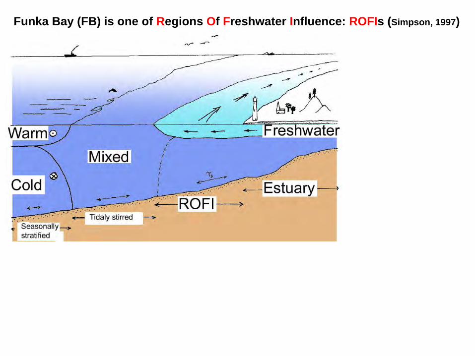
Funka Bay (FB) is one of Regions Of Freshwater Influence: ROFIs (Simpson, 1997)

Funka Bay (FB) is one of Regions Of Freshwater Influence: ROFIs (Simpson, 1997)

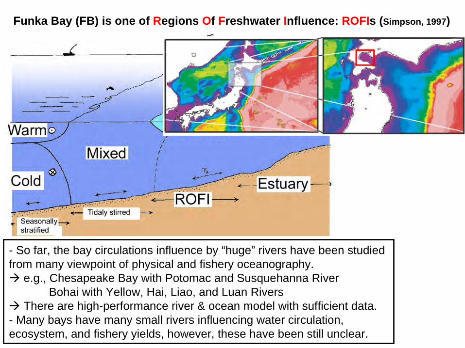
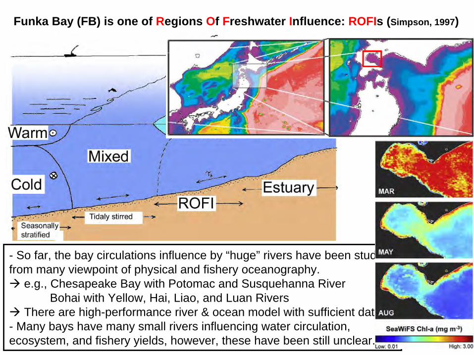
- So far, the bay circulations influence by “huge” rivers have been studied from many viewpoint of physical and fishery oceanography.

e.g., Chesapeake Bay with Potomac and Susquehanna RiverBohai with Yellow, Hai, Liao, and Luan Rivers

There are high-performance river & ocean model with sufficient data. - Many bays have many small rivers influencing water circulation, ecosystem, and fishery yields, however, these have been still unclear.

Funka Bay (FB) is one of Regions Of Freshwater Influence: ROFIs (Simpson, 1997)

- So far, the bay circulations influence by “huge” rivers have been studied from many viewpoint of physical and fishery oceanography.

e.g., Chesapeake Bay with Potomac and Susquehanna RiverBohai with Yellow, Hai, Liao, and Luan Rivers

There are high-performance river & ocean model with sufficient data. - Many bays have many small rivers influencing water circulation, ecosystem, and fishery yields, however, these have been still unclear.

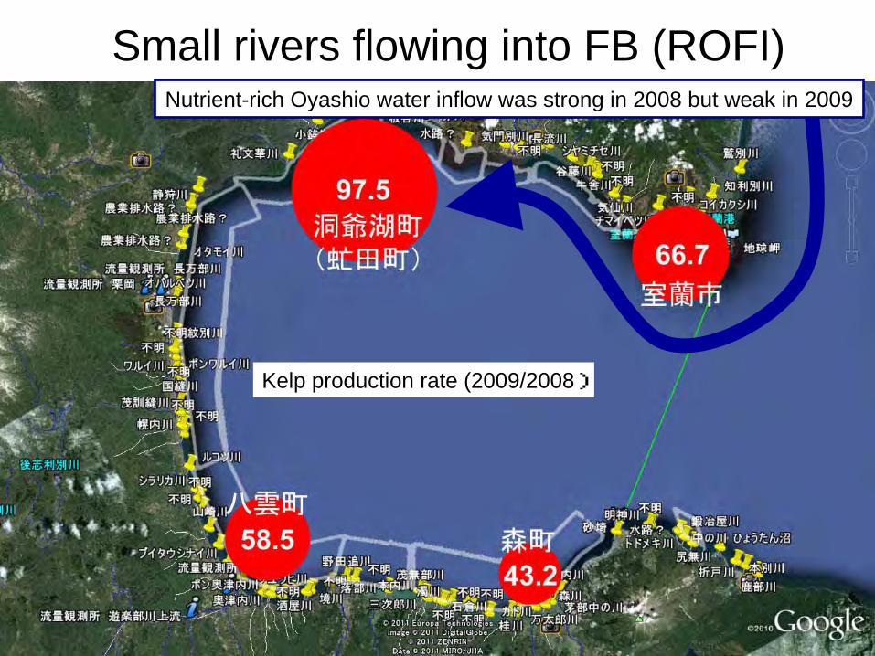
Small rivers flowing into FB (ROFI)

Kelp production rate (2009/2008）

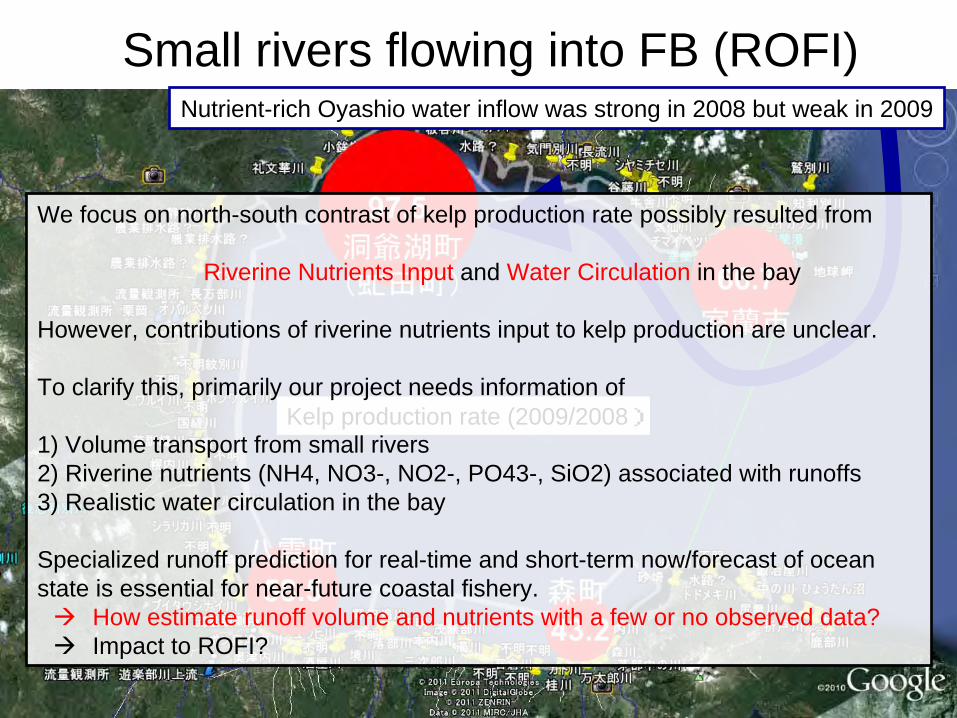
Nutrient-rich Oyashio water inflow was strong in 2008 but weak in 2009

Small rivers flowing into FB (ROFI)

Kelp production rate (2009/2008）

We focus on north-south contrast of kelp production rate possibly resulted from

Riverine Nutrients Input and Water Circulation in the bay

However, contributions of riverine nutrients input to kelp production are unclear.

To clarify this, primarily our project needs information of

1) Volume transport from small rivers2) Riverine nutrients (NH4, NO3-, NO2-, PO43-, SiO2) associated with runoffs3) Realistic water circulation in the bay

Specialized runoff prediction for real-time and short-term now/forecast of ocean state is essential for near-future coastal fishery.

How estimate runoff volume and nutrients with a few or no observed data?Impact to ROFI?

Nutrient-rich Oyashio water inflow was strong in 2008 but weak in 2009

Objectives

1) We propose procedures to estimate runoffs from small watersheds using meteorological data archiving low computational cost.

2) An application of locally coupled land-sea model are shown using the runoff model and OGCM around the FB.

3) By using the coupled model, we estimate nutrients loaded from river or land and understand relationship among nutrient inputs, kelp production, and water circulation by a numerical approach.

Numerical procedures

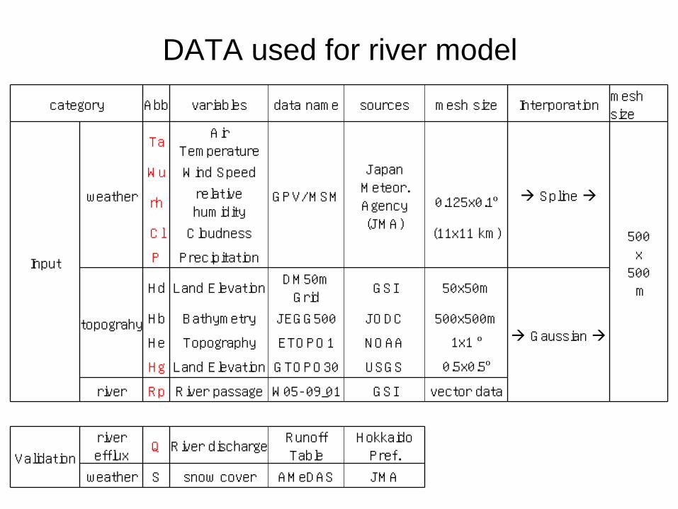
DATA used for river modelcategory Abb variables data name sources mesh size Interporation

mesh size

Input

weather

TaAir

Temperature

GPV/MSM

Japan

Meteor.

Agency

(JMA)

Spline

500

x

500

m

Wu Wind Speed

rhrelative humidity

0.125x0.1º

Cl Cloudness (11x11 km)

P Precipitation

topograhy

Hd Land ElevationDM50m Grid

GSI 50x50m

Gaussian Hb Bathymetry JEGG500 JODC 500x500m

He Topography ETOPO1 NOAA 1x1 º

Hg Land Elevation GTOPO30 USGS 0.5x0.5º

river Rp River passage W05-09_01 GSI vector data

Validation

river efflux

Q River dischargeRunoff

Table

HokkaidoPref.

weather S snow cover AMeDAS JMA

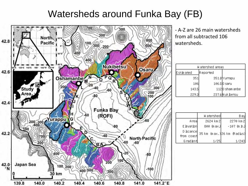
Watersheds around Funka Bay (FB)‐

A‐Z are 26 main watersheds 

from all subtracted 106 

watersheds.  

Watershed areas

Estimated Reported

351 351.8Yurrapu

106 106.5Osaru

143.5 112Oshamanbe

229.3 237.6Nukibetsu

Watershed Bay

Area 2624 km2 2270 km2

Elevation 800 (max.) -107 (min.)

Discance

from coast35 km (max. ) 26 km (Radius)

Gradient 1/25 1/243

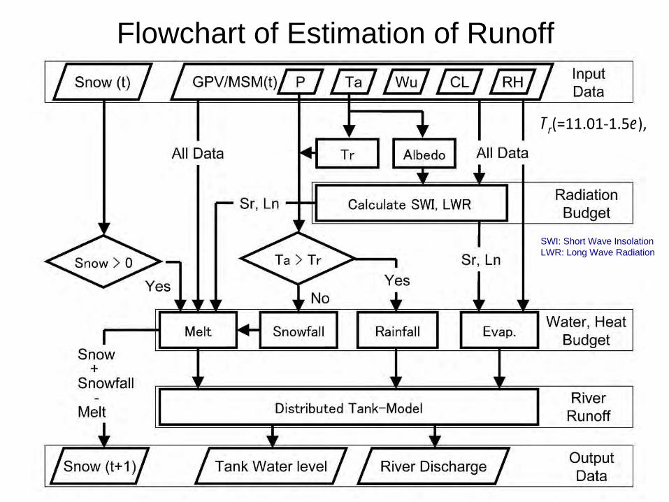
Flowchart of Estimation of Runoff

Tr (=11.01‐1.5e), 

SWI: Short Wave InsolationLWR: Long Wave Radiation

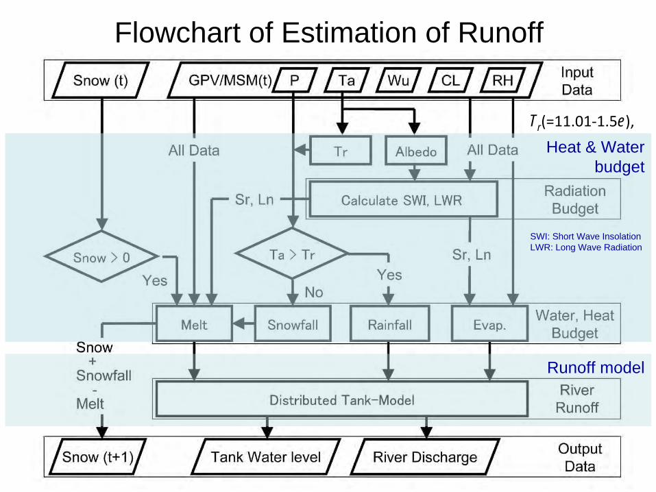
Flowchart of Estimation of Runoff

Tr (=11.01‐1.5e), 

Heat & Water budget

Runoff model

SWI: Short Wave InsolationLWR: Long Wave Radiation

Schematics of Radiation, Heat, and Water Budget- Radiation BudgetS↓: solar insolationS↑: reflected insolationL↓: downward radiation from sky and cloudL↑: upward radiation from surfaces

Rn = S↓

- S↑

+ L↓

- L↑

- Heat BudgetH: sensible heat fluxlE: latent heat fluxG: heat flux though ground surface

Rn-G=H+lE

- Water Budget R = P – E + M(snow>0)

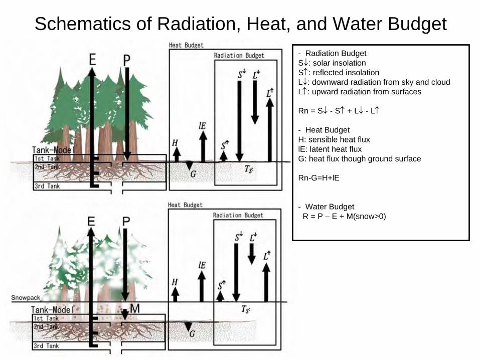
Schematics of Radiation, Heat, and Water Budget- Radiation BudgetS↓: solar insolationS↑: reflected insolationL↓: downward radiation from sky and cloudL↑: upward radiation from surfaces

Rn = S↓

- S↑

+ L↓

- L↑

- Heat BudgetH: sensible heat fluxlE: latent heat fluxG: heat flux though ground surface

Rn-G=H+lE

- Water Budget R = P – E + M(snow>0)

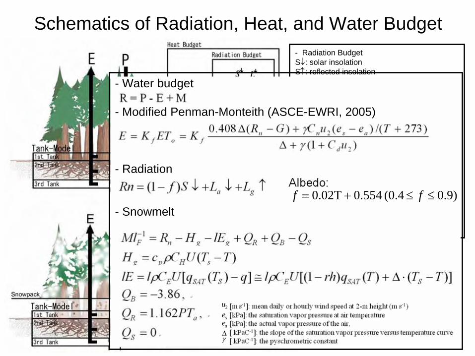
- Water budget

- Modified Penman-Monteith (ASCE-EWRI, 2005)

- Radiation

- Snowmelt0.9)(0.4 0.554 .02T0 ≤≤+= ff

2u

seaeΔγ

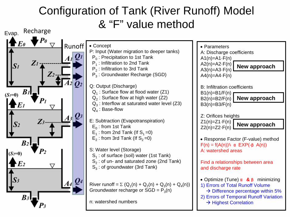
Configuration of Tank (River Runoff) Model & “F” value method

•

ConceptP: Input (Water migration to deeper tanks)

P0 : Precipitation to 1st TankP1 : Infiltration to 2nd TankP2 : Infiltration to 3rd TankP3 : Groundwater Recharge (SGD)

Q: Output (Discharge)Q1 : Surface flow at flood water (Z1)Q2 : Surface flow at high water (Z2)Q3 : Interflow at saturated water level (Z3)Q4 : Base-flow

E: Subtraction (Evapotranspiration)E0 : from 1st TankE1 : from 2nd Tank (If S1 =0)E2 : from 3rd Tank (If S2 =0)

S: Water level (Storage)S1 : of surface (soil) water (1st Tank)S2 : of un- and saturated zone (2nd Tank)S3 : of groundwater (3rd Tank)

River runoff = Σ

(Q1 (n) + Q2 (n) + Q3 (n) + Q4 (n))Groundwater recharge or SGD = P3 (n)

n: watershed numbers

•

ParametersA: Discharge coefficients A1(n)=A1·F(n)A2(n)=A2·F(n)A3(n)=A3·F(n)A4(n)=A4·F(n)

B: Infiltration coefficientsB1(n)=B1/F(n)B2(n)=B2/F(n)B3(n)=B3/F(n)

Z: Orifices heightsZ1(n)=Z1·F(n) Z2(n)=Z2·F(n)

•

Response Factor (F-value) methodF(n) = f(A(n))≒αEXP(-βA(n))A: watershed areas

Find a relationships between area and discharge rate

•

Optimize (Tune) α & β minimizing 1) Errors of Total Runoff Volume

Difference percentage within 5%2) Errors of Temporal Runoff Variation

Highest Correlation

Recharge

Runoff

New approach

New approach

New approach

Evap.

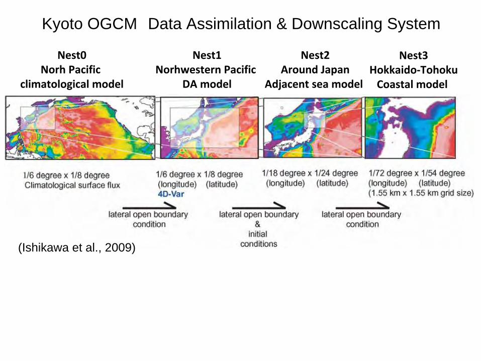
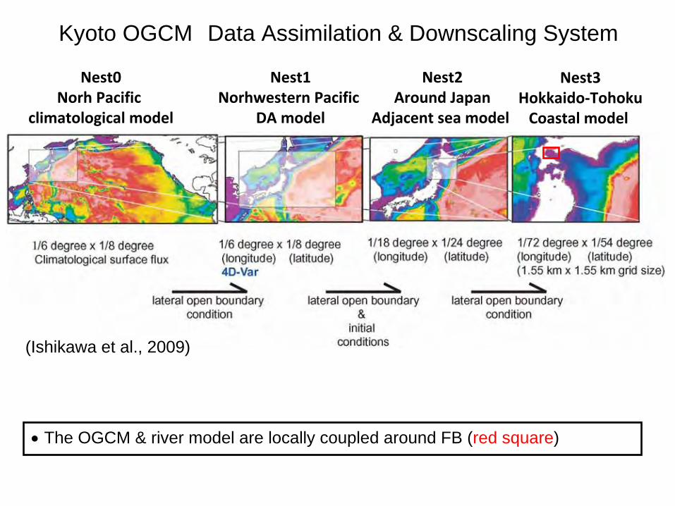
Kyoto OGCM Data Assimilation & Downscaling System

Nest0Norh

Pacific climatological model

Nest1Norhwestern

Pacific DA model

Nest2Around Japan

Adjacent sea model 

Nest3Hokkaido‐TohokuCoastal model 

(Ishikawa et al., 2009)

Kyoto OGCM Data Assimilation & Downscaling System

Nest0Norh

Pacific climatological model

Nest1Norhwestern

Pacific DA model

Nest2Around Japan

Adjacent sea model 

Nest3Hokkaido‐TohokuCoastal model 

•

The OGCM & river model are locally coupled around FB (red square)

(Ishikawa et al., 2009)

Results

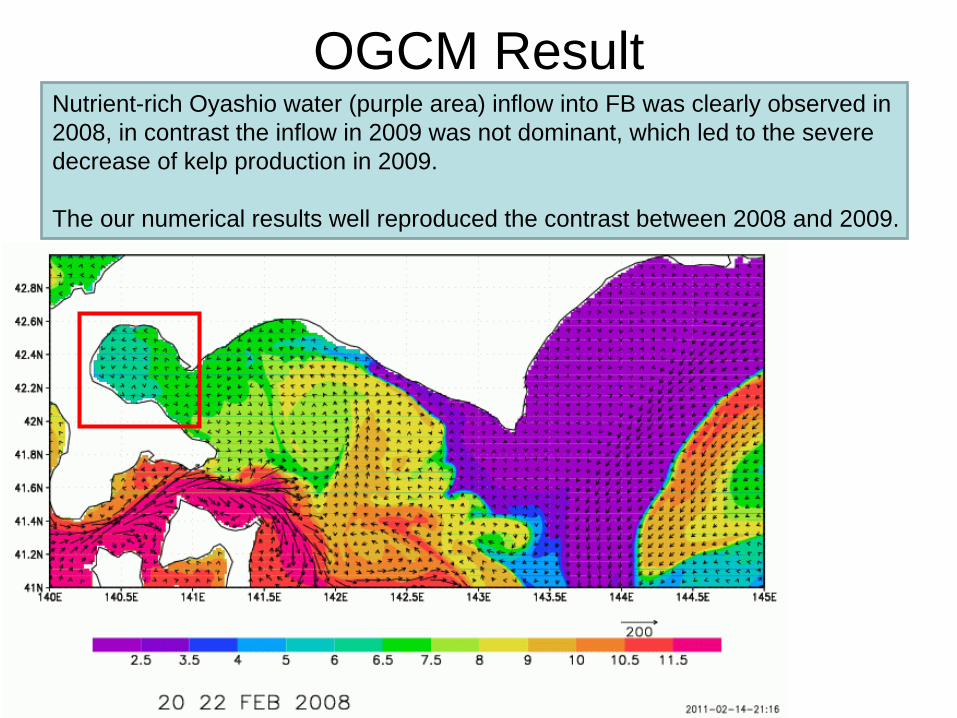
OGCM ResultNutrient-rich Oyashio water (purple area) inflow into FB was clearly observed in 2008, in contrast the inflow in 2009 was not dominant, which led to the severe decrease of kelp production in 2009.

The our numerical results well reproduced the contrast between 2008 and 2009.

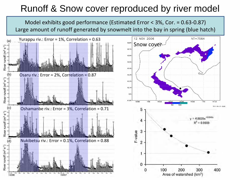
Runoff & Snow cover reproduced by river model

Yurappu

riv.: Error = 1%, Correlation = 0.63

Osaru

riv.: Error = 2%, Correlation = 0.87

Oshamanbe

riv.: Error = 3%, Correlation = 0.71

Nukibetsu

riv.: Error = 0.1%, Correlation = 0.88

Snow cover

Model exhibits good performance (Estimated Error < 3%, Cor. = 0.63‐0.87)Large amount of runoff generated by snowmelt into the bay in spring (blue hatch)

●

○

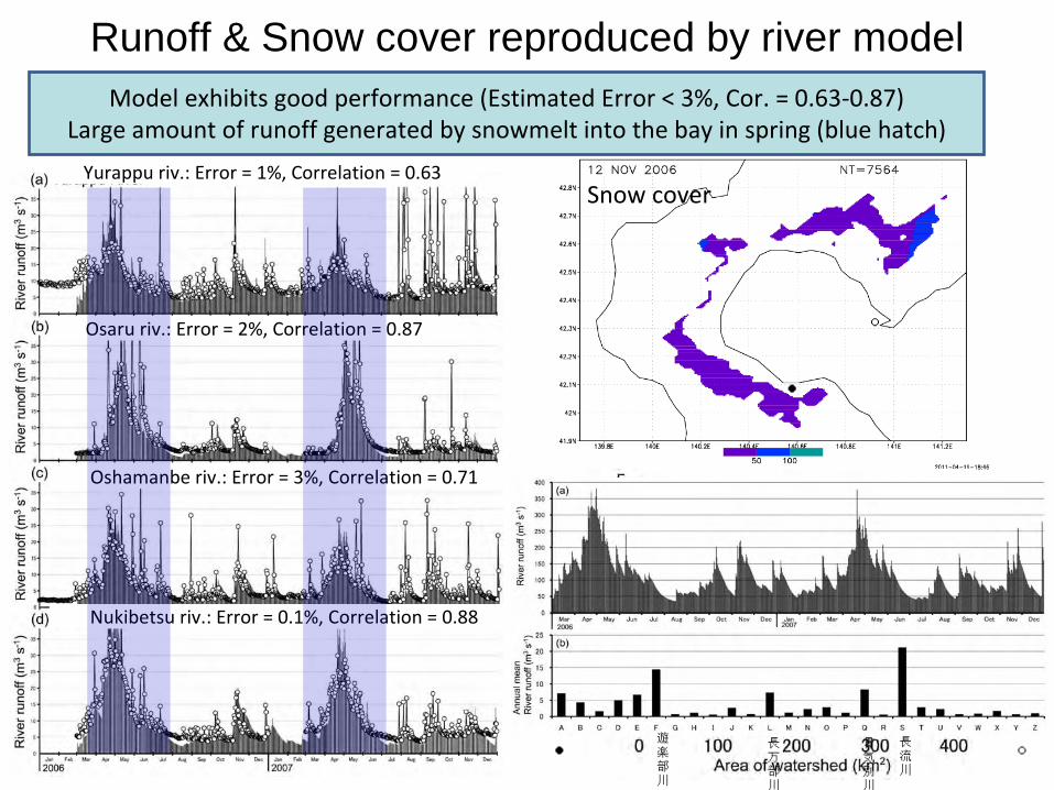
Runoff & Snow cover reproduced by river model

Yurappu

riv.: Error = 1%, Correlation = 0.63

Osaru

riv.: Error = 2%, Correlation = 0.87

Oshamanbe

riv.: Error = 3%, Correlation = 0.71

Nukibetsu

riv.: Error = 0.1%, Correlation = 0.88

Snow cover

● ○長

流

川

貫

気

別

川

長

万

部

川

遊

楽

部

川

Model exhibits good performance (Estimated Error < 3%, Cor. = 0.63‐0.87)Large amount of runoff generated by snowmelt into the bay in spring (blue hatch)

●

○

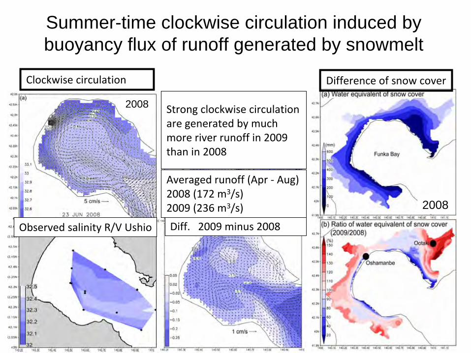
Summer-time clockwise circulation induced by buoyancy flux of runoff generated by snowmelt

河川モデルー月平均流量

Clockwise circulation

Observed salinity R/V Ushio Diff.

2009 minus 2008

Averaged runoff (Apr ‐

Aug)

2008 (172 m3/s) 

2009 (236 m3/s) 

Strong clockwise circulation 

are generated by much 

more river runoff in 2009 

than in 2008

Difference of snow cover

2008

2008

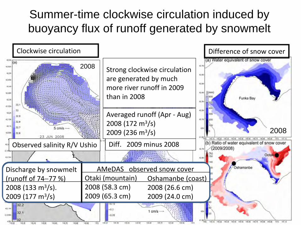
Summer-time clockwise circulation induced by buoyancy flux of runoff generated by snowmelt

河川モデルー月平均流量

Clockwise circulation

Observed salinity R/V Ushio Diff.

2009 minus 2008

Averaged runoff (Apr ‐

Aug)

2008 (172 m3/s) 

2009 (236 m3/s) 

Strong clockwise circulation 

are generated by much 

more river runoff in 2009 

than in 2008

Difference of snow cover

AMeDAS

observed snow coverOtaki

(mountain)2008 (58.3 cm)2009 (65.3 cm) 

Discharge by snowmelt

(runoff of 74−77 %)

2008 (133 m3/s). 2009 (177 m3/s)

Oshamanbe

(coast)2008 (26.6 cm)2009 (24.0 cm) 

2008

2008

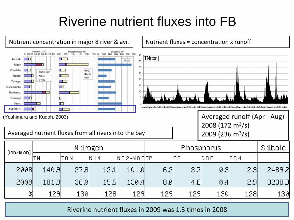
Riverine nutrient fluxes into FB

Riverine

nutrient fluxes in 2009 was 1.3 times in 2008

Nutrient concentration in major 8 river & avr. Nutrient fluxes = concentration x runoff

Averaged nutrient fluxes from all rivers into the bay

[ton/mon]Nitrogen Phosphorus Silicate

TN TON NH4 NO2+NO3TP PP DOP PO4

2008 140.9 27.8 12.1 101.0 6.2 3.7 0.3 2.3 2489.2

2009 181.9 36.0 15.5 130.4 8.0 4.8 0.4 2.9 3238.3

% 129 130 128 129 129 129 130 128 130

(Yoshimura and Kudoh, 2003) Averaged runoff (Apr ‐

Aug)

2008 (172 m3/s) 

2009 (236 m3/s) 

Speculation & Summary

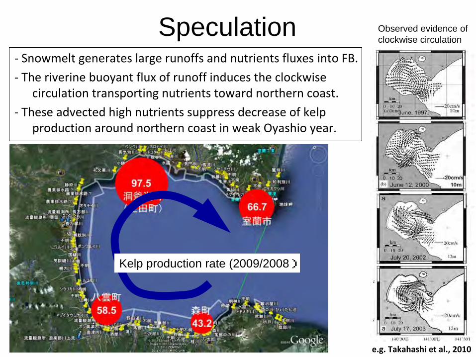
Speculation‐

Snowmelt generates large runoffs and nutrients fluxes

into FB.‐

The riverine

buoyant flux of runoff induces the clockwise 

circulation transporting nutrients toward northern coast.‐

These advected high nutrients suppress decrease of kelp 

production around northern coast in weak Oyashio

year.

Kelp production rate (2009/2008）

e.g. Takahashi et al., 2010

Observed evidence of clockwise circulation

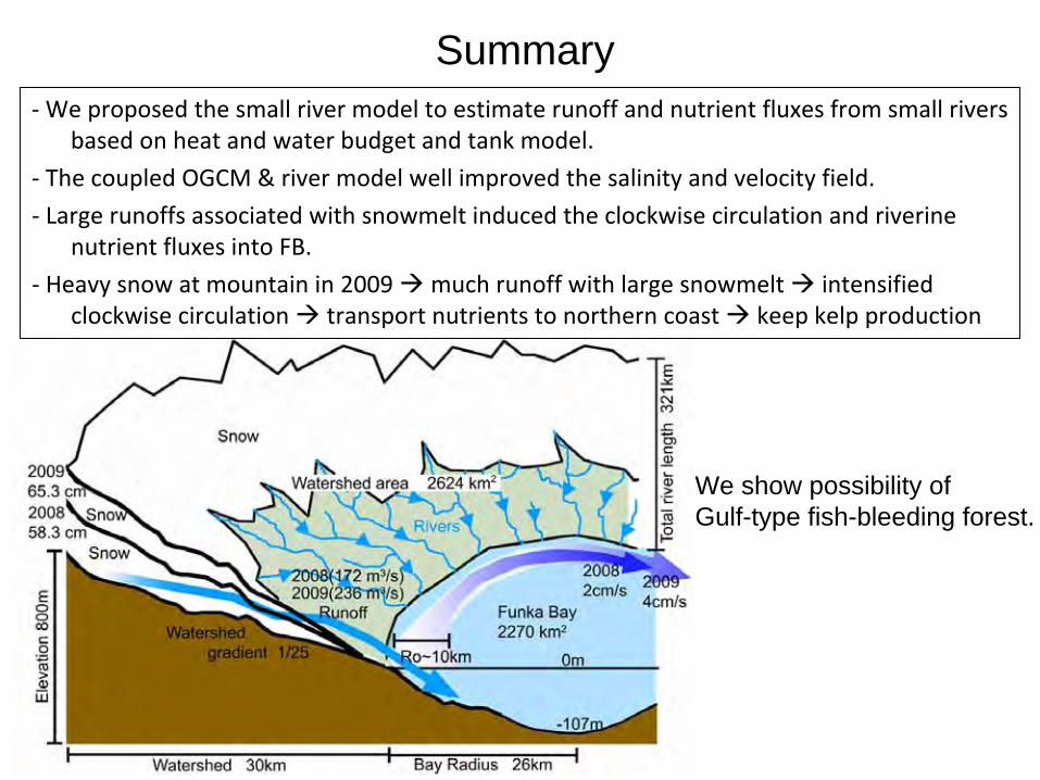
Summary‐

We proposed the small river model to estimate runoff and nutrient fluxes from small rivers 

based on heat and water budget and tank model.

‐

The coupled OGCM & river model well improved the salinity and velocity field. ‐

Large runoffs associated with snowmelt induced the clockwise circulation and riverine

nutrient fluxes into FB.

‐

Heavy snow at mountain in 2009  much runoff with large snowmelt  intensified clockwise circulation  transport nutrients to northern coast  keep kelp production

We show possibility ofGulf-type fish-bleeding forest.

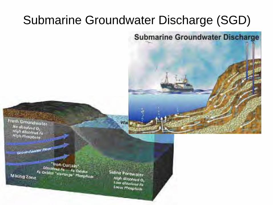
Submarine Groundwater Discharge (SGD)

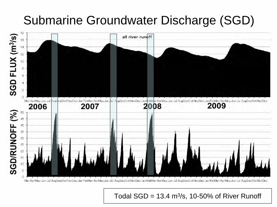
Submarine Groundwater Discharge (SGD)

Todal SGD = 13.4 m3/s, 10-50% of River Runoff