sas/gis 9.4: spatial data and procedure guide · pdf filethe correct bibliographic citation...
TRANSCRIPT

SAS/GIS® 9.4: Spatial Data and Procedure Guide
SAS® Documentation

The correct bibliographic citation for this manual is as follows: SAS Institute Inc. 2013. SAS/GIS® 9.4: Spatial Data and Procedure Guide. Cary, NC: SAS Institute Inc.
SAS/GIS® 9.4: Spatial Data and Procedure Guide
Copyright © 2013, SAS Institute Inc., Cary, NC, USA
All rights reserved. Produced in the United States of America.
For a hardcopy book:No part of this publication may be reproduced, stored in a retrieval system, or transmitted, in any form or by any means, electronic, mechanical, photocopying, or otherwise, without the prior written permission of the publisher, SAS Institute Inc.
For a Web download or e-book:Your use of this publication shall be governed by the terms established by the vendor at the time you acquire this publication.
The scanning, uploading, and distribution of this book via the Internet or any other means without the permission of the publisher is illegal and punishable by law. Please purchase only authorized electronic editions and do not participate in or encourage electronic piracy of copyrighted materials. Your support of others' rights is appreciated.
U.S. Government Restricted Rights Notice: Use, duplication, or disclosure of this software and related documentation by the U.S. government is subject to the Agreement with SAS Institute and the restrictions set forth in FAR 52.227–19 Commercial Computer Software-Restricted Rights (June 1987).
SAS Institute Inc., SAS Campus Drive, Cary, North Carolina 27513.
Electronic book 1, June 2013
SAS® Publishing provides a complete selection of books and electronic products to help customers use SAS software to its fullest potential. For more information about our e-books, e-learning products, CDs, and hard-copy books, visit the SAS Publishing Web site at support.sas.com/publishing or call 1-800-727-3228.
SAS® and all other SAS Institute Inc. product or service names are registered trademarks or trademarks of SAS Institute Inc. in the USA and other countries. ® indicates USA registration.
Other brand and product names are registered trademarks or trademarks of their respective companies.
Contents
About This Book . . . . . . . . . . . . . . . . . . . . . . . . . . . . . . . . . . . . . . . . . . . . . . . . . . . . . . . . vWhat’s New in SAS/GIS 9.4 . . . . . . . . . . . . . . . . . . . . . . . . . . . . . . . . . . . . . . . . . . . . . . viiRecommended Reading . . . . . . . . . . . . . . . . . . . . . . . . . . . . . . . . . . . . . . . . . . . . . . . . . . ix
Chapter 1 • Overview of SAS/GIS Software . . . . . . . . . . . . . . . . . . . . . . . . . . . . . . . . . . . . . . . . . . 1Introduction to Geographic Information Systems . . . . . . . . . . . . . . . . . . . . . . . . . . . . . . 1Features of SAS Software . . . . . . . . . . . . . . . . . . . . . . . . . . . . . . . . . . . . . . . . . . . . . . . . . 2Data in SAS/GIS Applications . . . . . . . . . . . . . . . . . . . . . . . . . . . . . . . . . . . . . . . . . . . . . 2Using the SAS/GIS Interface . . . . . . . . . . . . . . . . . . . . . . . . . . . . . . . . . . . . . . . . . . . . . . 8Accessing the SAS/GIS Tutorial . . . . . . . . . . . . . . . . . . . . . . . . . . . . . . . . . . . . . . . . . . 10
Chapter 2 • Preparing Spatial Data . . . . . . . . . . . . . . . . . . . . . . . . . . . . . . . . . . . . . . . . . . . . . . . . 11Assessing Your Spatial Data Needs . . . . . . . . . . . . . . . . . . . . . . . . . . . . . . . . . . . . . . . . 11Downloading TIGER/Line Spatial Data Files . . . . . . . . . . . . . . . . . . . . . . . . . . . . . . . . 13Examples of Common Spatial Data Tasks . . . . . . . . . . . . . . . . . . . . . . . . . . . . . . . . . . . 16Changing the Default Characteristics of a Map . . . . . . . . . . . . . . . . . . . . . . . . . . . . . . . 18Linking the Attribute Data to the Spatial Data . . . . . . . . . . . . . . . . . . . . . . . . . . . . . . . . 22Saving the Map Characteristics . . . . . . . . . . . . . . . . . . . . . . . . . . . . . . . . . . . . . . . . . . . 23
Chapter 3 • Importing Spatial Data . . . . . . . . . . . . . . . . . . . . . . . . . . . . . . . . . . . . . . . . . . . . . . . . 25Overview of Importing Spatial Data . . . . . . . . . . . . . . . . . . . . . . . . . . . . . . . . . . . . . . . . 25The GIS Spatial Data Importing Window . . . . . . . . . . . . . . . . . . . . . . . . . . . . . . . . . . . 26Common Importing Procedures . . . . . . . . . . . . . . . . . . . . . . . . . . . . . . . . . . . . . . . . . . . 29Importing ArcInfo Interchange Data . . . . . . . . . . . . . . . . . . . . . . . . . . . . . . . . . . . . . . . 30Importing DLG Data . . . . . . . . . . . . . . . . . . . . . . . . . . . . . . . . . . . . . . . . . . . . . . . . . . . . 31Importing DXF Data . . . . . . . . . . . . . . . . . . . . . . . . . . . . . . . . . . . . . . . . . . . . . . . . . . . . 32Importing Dynamap Data . . . . . . . . . . . . . . . . . . . . . . . . . . . . . . . . . . . . . . . . . . . . . . . . 32Importing MapInfo Data . . . . . . . . . . . . . . . . . . . . . . . . . . . . . . . . . . . . . . . . . . . . . . . . . 33Importing SAS/GRAPH Map Data Sets . . . . . . . . . . . . . . . . . . . . . . . . . . . . . . . . . . . . . 34Importing TIGER Data . . . . . . . . . . . . . . . . . . . . . . . . . . . . . . . . . . . . . . . . . . . . . . . . . . 35Importing Generic Spatial Data . . . . . . . . . . . . . . . . . . . . . . . . . . . . . . . . . . . . . . . . . . . 37Defining Composites in Imported Data . . . . . . . . . . . . . . . . . . . . . . . . . . . . . . . . . . . . . 40Defining Layers in Imported Data . . . . . . . . . . . . . . . . . . . . . . . . . . . . . . . . . . . . . . . . . 42The SASHELP.GISIMP Data Set . . . . . . . . . . . . . . . . . . . . . . . . . . . . . . . . . . . . . . . . . . 43
Chapter 4 • Batch Importing . . . . . . . . . . . . . . . . . . . . . . . . . . . . . . . . . . . . . . . . . . . . . . . . . . . . . 45Overview of Batch Importing . . . . . . . . . . . . . . . . . . . . . . . . . . . . . . . . . . . . . . . . . . . . . 45The Batch Import Process . . . . . . . . . . . . . . . . . . . . . . . . . . . . . . . . . . . . . . . . . . . . . . . . 46Examples of Batch Importing . . . . . . . . . . . . . . . . . . . . . . . . . . . . . . . . . . . . . . . . . . . . . 52File Reference Table for Batch Importing . . . . . . . . . . . . . . . . . . . . . . . . . . . . . . . . . . . 56TIGER 2007 – Present Shapefile Variables for the FACES File Type . . . . . . . . . . . . . 57Hints and Tips for Batch Importing . . . . . . . . . . . . . . . . . . . . . . . . . . . . . . . . . . . . . . . . 58
Chapter 5 • Working with Spatial Data . . . . . . . . . . . . . . . . . . . . . . . . . . . . . . . . . . . . . . . . . . . . . 61SAS/GIS Data Sets . . . . . . . . . . . . . . . . . . . . . . . . . . . . . . . . . . . . . . . . . . . . . . . . . . . . . 61Data Set and Catalog Entry Interactions . . . . . . . . . . . . . . . . . . . . . . . . . . . . . . . . . . . . . 69Merging Spatial Data with the MERGE= Argument . . . . . . . . . . . . . . . . . . . . . . . . . . . 74Sample SAS/GIS Spatial Database . . . . . . . . . . . . . . . . . . . . . . . . . . . . . . . . . . . . . . . . . 75Hints and Tips for Working with Spatial Data . . . . . . . . . . . . . . . . . . . . . . . . . . . . . . . . 75

Chapter 6 • Batch Geocoding . . . . . . . . . . . . . . . . . . . . . . . . . . . . . . . . . . . . . . . . . . . . . . . . . . . . 77Overview of Batch Geocoding . . . . . . . . . . . . . . . . . . . . . . . . . . . . . . . . . . . . . . . . . . . . 77Addresses in Spatial Data . . . . . . . . . . . . . . . . . . . . . . . . . . . . . . . . . . . . . . . . . . . . . . . . 78Using Batch Geocoding . . . . . . . . . . . . . . . . . . . . . . . . . . . . . . . . . . . . . . . . . . . . . . . . . 79How Batch Geocoding Works . . . . . . . . . . . . . . . . . . . . . . . . . . . . . . . . . . . . . . . . . . . . 79%GCBATCH Macro Statement . . . . . . . . . . . . . . . . . . . . . . . . . . . . . . . . . . . . . . . . . . . 83Batch Geocoding Example . . . . . . . . . . . . . . . . . . . . . . . . . . . . . . . . . . . . . . . . . . . . . . . 85Hints and Tips for Batch Geocoding . . . . . . . . . . . . . . . . . . . . . . . . . . . . . . . . . . . . . . . 88
Chapter 7 • The GIS Procedure . . . . . . . . . . . . . . . . . . . . . . . . . . . . . . . . . . . . . . . . . . . . . . . . . . . 91Overview: GIS Procedure . . . . . . . . . . . . . . . . . . . . . . . . . . . . . . . . . . . . . . . . . . . . . . . . 91Concepts: GIS Procedure . . . . . . . . . . . . . . . . . . . . . . . . . . . . . . . . . . . . . . . . . . . . . . . . 92Syntax: The GIS Procedure . . . . . . . . . . . . . . . . . . . . . . . . . . . . . . . . . . . . . . . . . . . . . . 94
Appendix 1 • Sample Map Data Sets . . . . . . . . . . . . . . . . . . . . . . . . . . . . . . . . . . . . . . . . . . . . . . 171Map and Data Sets Supplied with SAS/GIS Software . . . . . . . . . . . . . . . . . . . . . . . . . 171Maps in the USA Catalog . . . . . . . . . . . . . . . . . . . . . . . . . . . . . . . . . . . . . . . . . . . . . . . 171Maps in the NC Catalog . . . . . . . . . . . . . . . . . . . . . . . . . . . . . . . . . . . . . . . . . . . . . . . . 173Maps in the WAKE Catalog . . . . . . . . . . . . . . . . . . . . . . . . . . . . . . . . . . . . . . . . . . . . . 174Copying and Modifying SAS/GIS Maps in the MAPS or MAPSSAS Library . . . . . . 175Maps Produced by the SAS/GIS Tutorial . . . . . . . . . . . . . . . . . . . . . . . . . . . . . . . . . . . 176
Appendix 2 • Spatial Database Details . . . . . . . . . . . . . . . . . . . . . . . . . . . . . . . . . . . . . . . . . . . . 179The SAS/GIS Data Model . . . . . . . . . . . . . . . . . . . . . . . . . . . . . . . . . . . . . . . . . . . . . . 179SAS/GIS Spatial Database Structure . . . . . . . . . . . . . . . . . . . . . . . . . . . . . . . . . . . . . . 182Composites . . . . . . . . . . . . . . . . . . . . . . . . . . . . . . . . . . . . . . . . . . . . . . . . . . . . . . . . . . 190
Appendix 3 • Calculating Chain Rank . . . . . . . . . . . . . . . . . . . . . . . . . . . . . . . . . . . . . . . . . . . . . 191RANK Value Equation . . . . . . . . . . . . . . . . . . . . . . . . . . . . . . . . . . . . . . . . . . . . . . . . . 191Chain Rank Calculation Examples . . . . . . . . . . . . . . . . . . . . . . . . . . . . . . . . . . . . . . . . 195
Glossary . . . . . . . . . . . . . . . . . . . . . . . . . . . . . . . . . . . . . . . . . . . . . . . . . . . . . 199Index . . . . . . . . . . . . . . . . . . . . . . . . . . . . . . . . . . . . . . . . . . . . . . . . . . . . . . . . 205
iv Contents

About This Book
Using This Document
PrerequisiteThis document is written for users who want to use the SAS/GIS geographic information system to explore data in the context of a map. You must have a map in order to use SAS/GIS software. Furthermore, the map must be in a spatial data format that SAS/GIS software can use.
This document is written for users who are experienced in using the SAS System. You should understand the concepts of programming in the SAS language. The following table summarizes the SAS System concepts that you need to understand in order to use SAS/GIS.
Task Reference
Invoke the SAS System at your site Instructions provided by the on-site SAS support personnel
Use Base SAS software
Use the DATA step to create and manipulate SAS data sets
Use the SAS windowing environment or SAS Enterprise Guide to enter, edit, and submit program code
Base documentation library:
• SAS Language Reference: Concepts
• SAS Data Set Options: Reference
• SAS Formats and Informats: Reference
• SAS Functions and CALL Routines: Reference
• SAS Statements: Reference
• SAS System Options: Reference
• Base SAS Utilities: Reference
Allocate SAS libraries and assign librefs
Create external files and assign filerefs
Documentation for using the SAS System in your operating environment:
• SAS Companion for Windows
• SAS Companion for UNIX Environments
• SAS Companion for z/OS
Manipulate SAS data sets using SAS procedures
Base SAS Procedures Guide
v

Particular fonts have special meanings when used in the presentation of SAS/GIS syntax in this document. For example, items presented in italics identify arguments or values that you supply. Angle brackets (< >) indicate optional arguments. The conventions used in this document are the same conventions used in Base SAS documentation. For a complete explanation, see the Base SAS documentation listed above.
Map Data SetsTo draw maps, you need to know where the map data sets are stored on your system. Depending on your installation, the map data set might automatically be assigned a libref. Ask your on-site SAS support personnel or system administrator where the map data sets are stored for your site.
vi About This Book

What’s New in SAS/GIS 9.4
Overview
There is an important new import capability in SAS/GIS 9.4. You can now import TIGER shapefiles (.shp) that fall in the date range of 2007 to the present. This import function can be run interactively or programmatically. The import method for TIGER/Line record type (RT format) files created prior to 2007 remains intact.
Changes to Importing TIGER Data
SAS/GIS, through the GIS Spatial Data Importing window, allows the interactive import of spatial data in the Topologically Integrated Geographic Encoding and Referencing (TIGER) format. The import capability covered any spatial data in the RT format created prior to 2007. With the release of 9.4, the import capability of SAS/GIS is expanded to include the TIGER shapefile (.shp) file format that was created starting in the year 2007. You have the option of importing any shapefile either programmatically or interactively through the GIS Spatial Data Importing window.
vii

viii What’s New in SAS/GIS 9.4

Recommended Reading
• SAS/ACCESS for Relational Databases: Reference
• SAS/FSP: Procedures Guide
• SAS/GRAPH: Reference
• SAS Language Reference: Concepts
• SAS Statements: Reference
• SAS Data Set Options: Reference
• SAS System Options: Reference
• Base SAS Procedures Guide
• SAS Companion that is specific to your operating environment
For a complete list of SAS books, go to support.sas.com/bookstore. If you have questions about which titles you need, please contact a SAS Book Sales Representative:
SAS BooksSAS Campus DriveCary, NC 27513-2414Phone: 1-800-727-3228Fax: 1-919-677-8166E-mail: [email protected] address: support.sas.com/bookstore
ix

x Recommended Reading

Chapter 1
Overview of SAS/GIS Software
Introduction to Geographic Information Systems . . . . . . . . . . . . . . . . . . . . . . . . . . . . 1
Features of SAS Software . . . . . . . . . . . . . . . . . . . . . . . . . . . . . . . . . . . . . . . . . . . . . . . 2
Data in SAS/GIS Applications . . . . . . . . . . . . . . . . . . . . . . . . . . . . . . . . . . . . . . . . . . . . 2SAS/GIS Data Types . . . . . . . . . . . . . . . . . . . . . . . . . . . . . . . . . . . . . . . . . . . . . . . . . 2Spatial Data . . . . . . . . . . . . . . . . . . . . . . . . . . . . . . . . . . . . . . . . . . . . . . . . . . . . . . . . . 3Attribute Data . . . . . . . . . . . . . . . . . . . . . . . . . . . . . . . . . . . . . . . . . . . . . . . . . . . . . . . 5Designing a SAS/GIS Spatial Database . . . . . . . . . . . . . . . . . . . . . . . . . . . . . . . . . . . 6
Using the SAS/GIS Interface . . . . . . . . . . . . . . . . . . . . . . . . . . . . . . . . . . . . . . . . . . . . . 8Starting SAS/GIS Software . . . . . . . . . . . . . . . . . . . . . . . . . . . . . . . . . . . . . . . . . . . . 8Using Dialog Box Elements . . . . . . . . . . . . . . . . . . . . . . . . . . . . . . . . . . . . . . . . . . . . 8Selecting Maps and SAS Data Sets . . . . . . . . . . . . . . . . . . . . . . . . . . . . . . . . . . . . . . 9
Accessing the SAS/GIS Tutorial . . . . . . . . . . . . . . . . . . . . . . . . . . . . . . . . . . . . . . . . . 10
Introduction to Geographic Information SystemsSAS/GIS software provides an interactive geographic information system within SAS. A geographic information system (GIS) is a tool for organizing and analyzing data that can be referenced spatially, that is, data that can be tied to physical locations. Many types of data have a spatial aspect, including demographics, marketing surveys, customer addresses, and epidemiological studies. A GIS helps you analyze your data in the context of location.
For example, if you need to evaluate population data for census tracts, you could view the information in tabular format. However, consider how much easier and more effective it is to view the demographic information in the context of the geography of the tracts as shown in the following figure. When viewing information that has a spatial component, you might find it easier to recognize relationships and trends in your data if you view the information in a spatial context.
1

Figure 1.1 Evaluating Spatially Referenced Data
SAS/GIS software enables you to do more than simply view your data in its spatial context. It also enables you to interact with the data by selecting features and performing actions that are based on your selections. SAS/GIS software draws on the capabilities of SAS and enables you to access, manage, analyze, and present your data easily.
Features of SAS SoftwareSAS provides a powerful programming language with components called procedures. Procedures enable you to perform many different types of analysis and data management functions. Procedures also produce many different types of text-based and graphical presentation output. Combined with other features, the SAS language and its procedures make an immense variety of applications possible, including the following examples:
• Access raw data files and data in external databases and database management systems.
• Manage data using tools for data entry, editing, retrieval, formatting, and conversion.
• Analyze data using descriptive statistics, multivariate techniques, forecasting and modeling, and linear programming.
• Present data using reports and business and statistical graphics.
SAS is also portable across computing environments. SAS applications function the same and produce the same results regardless of the operating environment on which you are running SAS to process your data. However, some features, such as interactive windows, are not supported on all platforms.
For more information about SAS, refer to SAS Language Reference: Concepts.
Data in SAS/GIS Applications
SAS/GIS Data TypesSAS/GIS software uses two basic types of data:
2 Chapter 1 • Overview of SAS/GIS Software

spatial datacontains the coordinates and identifying information that describes the map features such as streets, rivers, and railroads.
attribute datais the information that you want to use for analysis or presentation. This information must be spatial in nature. Examples of information that is spatial in nature because the information applies to a specific geographic feature include the following:
• sales figures for each of your store locations
• population data for each county
• total income for each household in a region
For example, the U.S. Census Bureau distributes both types of data:
TIGER/Line shapefilescontain spatial information that you can use to build maps.
Summary Tape filescontain population and other demographic information that you can link to the map features.
Attribute data provides the information that you want to analyze, and spatial data provides the context in which you want to analyze it. For example, consider the SAS/GIS map shown in the following display. Spatial data provides the boundaries for the map areas, and attribute data provides the population information that is used to color the map areas.
Display 1.1 Spatial and Attribute Data in SAS/GIS Maps
Spatial Data
Overview of Spatial DataSpatial data contains the coordinates and identifying information that are necessary to draw maps. For SAS/GIS software, spatial data is stored in SAS/GIS spatial databases,
Data in SAS/GIS Applications 3

which consist of collections of SAS data sets and SAS catalog entries. The primary method for creating a SAS/GIS spatial database is through the SAS/GIS Import facility, either in batch or in interactive mode. You can also use the GIS procedure to create, modify, and manage the catalog entries in a spatial database.
Spatial Data LayersFeatures in the spatial data are organized into layers. A layer is a collection of all the features in the map that share some common characteristic. The various physical aspects of the map—political boundaries, roads, railroads, waterways, and so on—are assigned to layers according to their common spatial data values. Some features can appear in multiple layers. For example, a street can also be a ZIP code boundary and a city boundary line. The street could appear in three layers: one containing the streets, one containing the ZIP code boundaries, and one containing the city boundaries.
Three types of layers can be represented in SAS/GIS maps: points, lines, and areas. These are examples:
• The collection of all the points in a map that represent park locations can be organized into a point layer for parks.
• The collection of all the lines in a map that represent streets can be organized into a line layer for streets.
• The collection of all the areas that represent census tracts can be organized into an area layer for tracts.
When the various layers are overlaid, they form a map, as shown in the following figure.
Figure 1.2 Layers Forming a SAS/GIS Map
Point Layer (Parks)
Line Layer (Streets)
Area Layer (Tracts)
Resulting Map
A layer can be displayed as either static or thematic. When a layer is displayed as static, it uses the same graphical characteristics (color, line, width, and so on) for all features in that layer. For example, a street layer could use the same color and line style to display all the streets. When a layer is displayed as thematic, it uses different graphical characteristics to classify the features in that layer. For example, a theme representing sales regions could use different colors to show the quarterly sales performance of each region. A theme in a layer representing highways could use different line widths to show
4 Chapter 1 • Overview of SAS/GIS Software

the classes of roads. A layer can have multiple themes stored in it, and you can easily change which theme is currently displayed.
Spatial Data CoveragesIn SAS/GIS software, maps display only the portion of the spatial data that falls within a given coverage. A coverage defines a subset of the spatial data that is available to a map. The coverage can include all the spatial data in the database, or only selected portions. For example, a spatial database might contain geographic data for an entire country. However, a coverage might restrict the portion that is available for a given map to only one region. You can define more than one coverage for each spatial database, although a map uses only one coverage at a time.
Spatial Data CompositesMost operations in SAS/GIS software use composites of spatial data variables rather than the actual spatial data variables themselves. Composites identify the relationships and purpose of the variables in the spatial data.
For example, the spatial data can have the variables STATEL and STATER that contain the state ID codes for the left and right sides of each feature. In this case, the spatial database could define a composite named STATE that identifies the relationship between these variables. The spatial database could also specify that they delineate state areas in the map. You would use the STATE composite, rather than the actual STATEL and STATER variables, to link state areas in the map to attribute data for the corresponding state.
See Appendix 2, “Spatial Database Details,” on page 179 for more information about the structure of SAS/GIS spatial databases.
Attribute DataThe second type of data that is used in a GIS is attribute data. In SAS/GIS software, your attribute data must be stored in either a SAS data set or a SAS view. SAS views enable you to transparently access data in other formats. For example, you can create a SAS/ACCESS view to access data in a database such as DB2. A DATA step view or an SQL view also enables you to access an external file, or any other type of data from which you can create a SAS view. Once your attribute data is accessible either as a SAS data set or through a SAS view, it can be linked to your spatial data. The linked attribute data can then be used in labeling, analysis, or theming. For example, your spatial data might represent a county and contain information for city boundaries, census tract boundaries, streets, and so on. An attribute data set with population information for each census tract can be linked to a map using the corresponding tract composite in the spatial data.
Some of the ways in which you can use attribute data in SAS/GIS software include the following:
• Use values in your attribute data as labels. For example, you could use attribute data containing population data to provide the text of labels for census tracts.
• Use the values in your attribute data as themes for layers. For example, you could use attribute data containing average household income data as a theme for a census tract layer.
See Chapter 5, “Customizing Maps,” in SAS/GIS Software: Usage and Reference, Version 6 for more information about assigning themes to map layers.
• Define actions that display or manipulate the attribute data when features are selected in the map. In this way, you can explore your attribute data interactively
Data in SAS/GIS Applications 5

rather than simply view static results. The actions can range from simple to complex. A simple action can be displaying observations from an attribute data set that relate to features in the map. A complex action can be submitting a procedure from SAS/STAT software to perform a statistical analysis.
You can define the following actions for your attribute data:
• Display observations from attribute data sets that relate to selected map features.
• Open additional maps that relate to selected map features.
• Display images that relate to selected map features.
• Interactively subset attribute data sets according to a subset of selected map features.
• Submit SAS programs.
• Issue SAS commands.
• Issue host commands.
• Display and edit information for the selected map features.
• Organize area features into groups that are based on your attribute data.
See Chapter 4, “Performing Actions for Selected Map Features” in SAS/GIS Software: Usage and Reference, Version 6 for more information about defining and performing actions.
Designing a SAS/GIS Spatial Database
SAS/GIS Data TypesOne of the first steps in a SAS/GIS project is determining the design of your SAS/GIS spatial database. The database will contain the following types of information:
Table 1.1 SAS/GIS Data Types
Type of Data Database Contents
Spatial All of the spatial data that the user wants to see
Attribute All of the associated attribute data that the user needs to use for analysis or presentation purposes
Before you begin creating the spatial database, you should draw up an overview of the system goals and data requirements. The time you spend designing your database initially will save you time and expenses later in the project. A well-designed database is easier to maintain and document, and you can extend it for future GIS projects.
Use the following guidelines when determining the information that you want to include in a database:
6 Chapter 1 • Overview of SAS/GIS Software

Table 1.2 SAS/GIS Spatial Database Guidelines
Data Type Steps for Determining
Project objective 1. Identify the initial objective of the project and its ultimate goal.
2. Consider any requirements that might have been imposed on it.
3. Determine the feasibility of initial implementation and, as best as possible, the impact of any future demands.
Attribute data 1. Identify the attribute data that is necessary to illustrate the project objectives.
2. Determine whether you have this data or can obtain it.
Spatial data 1. Identify the spatial features that you need to link with your attribute data (for example, states, cities, rivers, roads, railroads, airports, and so on).
2. Determine whether you have this data or can obtain it.
Once you have determined a preliminary list of the data that you will need, use the additional factors in the following sections to help you evaluate and refine your list.
Enable Linking between Spatial Features and Attribute DataYou can use attribute data for map actions, themes, or labeling. However, the attribute data set must contain the same identification information as the spatial feature that it describes. This enables you to link between them. For example, your attribute data can have Sales Revenue for stores, and Store ID Numbers. You probably want to include the actual location in longitude and latitude for each Store ID Number on your spatial data list. You can then place a marker at the store location and also visualize and analyze the corresponding attribute data for each store.
Use No More Details Than You NeedUse only the data that you need for your project. For example, if you have store locations that request the customer ZIP code at the cash register, you should not assume that you need ZIP code boundaries on your map. ZIP code boundaries might be far too small for your purposes if you have stores nationwide. You might decide instead that the three-digit ZIP code boundaries provide fewer, yet more appropriately sized, areas for your analysis. You can summarize your attribute data to the three-digit ZIP code level and use it for your analysis. This reduces both the amount of spatial data and attribute data that you need. As long as it is appropriate for your analysis, decreasing the amount of required spatial and attribute data reduces storage space and improves performance. Reducing the level of detail in the spatial data also saves money if you have to purchase the data.
Ensure a Common Level of Spatial and Attribute DataYou can plan to summarize your attribute data to a matching level of your spatial data. You must make sure that the two types of data have a common level that you can use. For example, ZIP code boundaries can cross not only county boundaries, but also state boundaries. This means that there is usually not a one-to-one correspondence between ZIP codes and states or counties. For example, you might find that the only information
Data in SAS/GIS Applications 7

that ties your attribute data to your spatial data is ZIP codes. To avoid difficulties using your ZIP code level attribute data, include more than just state or county boundaries in your spatial data.
For specific, smaller areas of the country, a one-to-one correspondence might exist that will enable you to summarize your attribute data to a higher level. However, ZIP codes can change frequently, and this correspondence might be lost. Also, because ZIP codes change, you must be able to account for these changes when performing a historical analysis. For example, if you are comparing sales in a specific ZIP code area over a ten-year period, make sure that the area remained constant during that period. The same is true for other spatial data.
Using the SAS/GIS Interface
Starting SAS/GIS SoftwareUse the following steps to start a SAS/GIS software session:
1. Open a SAS session.
2. From the SAS menu bar, select Solutions ð Analysis ð Geographic Information System
Or type GIS in the SAS Command Box or on any SAS command line.
Using Dialog Box ElementsIn most places where you must supply a value in a SAS/GIS window, directions will guide you. They can take the form of a pull-out arrow, a drop-down arrow, or both, presented in conjunction with text boxes, as shown in the following display.
Display 1.2 Typical Dialog Box Elements
Clicking a drop-down arrow displays a list of valid choices for the option. Display 1.3 on page 8 shows the list that is displayed by clicking the drop-down arrow for the Style field in Display 1.2 on page 8.
Display 1.3 List Displayed by the Style Drop-down Arrow
8 Chapter 1 • Overview of SAS/GIS Software

Clicking a pull-out arrow opens a new window in which you can interactively select appropriate values. The following display shows the window that is opened by clicking the pull-out arrow for the Color field in Display 1.2 on page 8.
Display 1.4 Window That Is Opened by the Color Pull-out Arrow
Selecting Maps and SAS Data SetsWhenever you need to specify the name of a SAS data set or SAS catalog entry, SAS/GIS software opens an Open window like the one shown in the following display.
Display 1.5 Typical Open Window
The window provides an intuitive way to find the SAS data set or catalog entry that you need. It also makes it impossible to enter an invalid name, because only those choices that are appropriate for the operation that you are performing are presented for selection.
To select each level of the SAS name from the tree view, double-click your choice. Once you make a selection, the list of available choices for the next level of the name is displayed.
Using the SAS/GIS Interface 9

Accessing the SAS/GIS TutorialThis book does not attempt to cover all of the fundamentals of using SAS/GIS software. For an introduction to the basic tasks that you can perform, see the online tutorial that is included in SAS/GIS software. To start the tutorial, make the following selections from the GIS Map window's menu bar:
Help ð Getting Started with SAS/GIS Software ð Begin Tutorial
The tutorial creates sample maps and attribute data and leads you step by step through the following tasks:
• displaying maps
• selecting the types of feedback that are provided about the displayed map
• using the zoom tool to zoom in on selected areas of the map
• using the pan tool to move the map within the window
• modifying, adding, and removing layers in the map
• using attribute data as a theme for a layer
• adding legends that explain how features are represented
• selecting features and using actions to explore the attribute data
• saving changes to the map
• geocoding addresses
• adding points to a map
After you have used the online tutorial to become familiar with the basics of using SAS/GIS software, you can refer to SAS/GIS Software: Usage and Reference, Version 6 for additional information about using SAS/GIS software and for detailed reference information about the features of SAS/GIS software.
10 Chapter 1 • Overview of SAS/GIS Software

Chapter 2
Preparing Spatial Data
Assessing Your Spatial Data Needs . . . . . . . . . . . . . . . . . . . . . . . . . . . . . . . . . . . . . . . 11Determining Prerequisites . . . . . . . . . . . . . . . . . . . . . . . . . . . . . . . . . . . . . . . . . . . . 11Assessing Your Attribute Data . . . . . . . . . . . . . . . . . . . . . . . . . . . . . . . . . . . . . . . . . 11Determining Your Spatial Data Requirements . . . . . . . . . . . . . . . . . . . . . . . . . . . . . 12Locating a Source of Spatial Data . . . . . . . . . . . . . . . . . . . . . . . . . . . . . . . . . . . . . . 12
Downloading TIGER/Line Spatial Data Files . . . . . . . . . . . . . . . . . . . . . . . . . . . . . . 13Defining the Types of TIGER/Line Shapefiles Needed . . . . . . . . . . . . . . . . . . . . . . 13Required TIGER/Line Shapefile File Types . . . . . . . . . . . . . . . . . . . . . . . . . . . . . . 13Downloading TIGER/Line Record Type (RT) Files (1990 – 2006) . . . . . . . . . . . . 14Downloading TIGER/Line Shapefiles (.shp) (2007 – present) . . . . . . . . . . . . . . . . 15
Examples of Common Spatial Data Tasks . . . . . . . . . . . . . . . . . . . . . . . . . . . . . . . . . 16Overview of Common Spatial Data Tasks . . . . . . . . . . . . . . . . . . . . . . . . . . . . . . . . 16Importing Your Spatial Data . . . . . . . . . . . . . . . . . . . . . . . . . . . . . . . . . . . . . . . . . . 16
Changing the Default Characteristics of a Map . . . . . . . . . . . . . . . . . . . . . . . . . . . . 18Customizing Maps . . . . . . . . . . . . . . . . . . . . . . . . . . . . . . . . . . . . . . . . . . . . . . . . . . 18Selecting a Map Projection . . . . . . . . . . . . . . . . . . . . . . . . . . . . . . . . . . . . . . . . . . . . 19Selecting the Units System . . . . . . . . . . . . . . . . . . . . . . . . . . . . . . . . . . . . . . . . . . . . 20Selecting a Background Color . . . . . . . . . . . . . . . . . . . . . . . . . . . . . . . . . . . . . . . . . 20Choosing Which Layers Are Displayed . . . . . . . . . . . . . . . . . . . . . . . . . . . . . . . . . . 20Changing the Level of Detail . . . . . . . . . . . . . . . . . . . . . . . . . . . . . . . . . . . . . . . . . . 21
Linking the Attribute Data to the Spatial Data . . . . . . . . . . . . . . . . . . . . . . . . . . . . . 22
Saving the Map Characteristics . . . . . . . . . . . . . . . . . . . . . . . . . . . . . . . . . . . . . . . . . 23
Assessing Your Spatial Data Needs
Determining PrerequisitesYou use a geographic information system to explore data in the context of a map, so you must have a map in order to use SAS/GIS software. In addition, the map must be in the form of spatial data that SAS/GIS software can use.
Assessing Your Attribute DataThe first step in deciding what spatial data you need is to assess the attribute data that you want to analyze. The attribute data must have a spatial component. That is, the data
11

must contain at least one variable with values that relate to location. Examples include city, state, or country names or codes; street names; addresses; and so on. Because SAS/GIS software is part of SAS, the attribute data must also be in the form of a SAS data set or a SAS view. If needed, you can use any method that is available for transforming your attribute data into a SAS data set or a SAS view. These methods include, but are not limited to the following:
• using SAS programming statements or the SAS Import Wizard to read external files into SAS data sets
• using SAS/ACCESS software or the SQL procedure to create views to database files
• using SAS programming statements or the SQL procedure to create dynamic views to SAS data sets.
First ensure that your attribute data has a spatial component and is in a format that SAS/GIS can read. Then proceed to identify and locate your spatial data.
Determining Your Spatial Data RequirementsSAS/GIS software can analyze attribute data under certain conditions. You need spatial data that contains representations of features to at least the same level of detail as the location information in your attribute data. For example, if your attribute data consists of demographic data for states, then your spatial data must provide at least state boundaries. Your attribute data can consist of demographic data for smaller census tracts. You will then need spatial data that contains the corresponding census tract boundaries. Only then can SAS/GIS software explore the demographic data.
Locating a Source of Spatial DataTo acquire spatial data for use with SAS/GIS software, you import the data from other formats. One readily accessible source of maps for importing is the map data sets that are provided with SAS/GRAPH software. However, these maps provide only political boundaries and not other physical features such as rivers and major highways. Other sources for spatial data that you can import include the following:
• Governmental agencies. For example, SAS/GIS software can import spatial data from TIGER/Line shapefiles produced by the U.S. Census Bureau and from DLG files produced by the U.S. Geological Survey.
• Drawing and computer-aided design (CAD) packages. SAS/GIS software can import the DXF interchange format that is supported by products from various vendors.
• Tele Atlas N.V. SAS/GIS can import the Dynamap files.
• MapInfo Corporation. SAS/GIS can import MapInfo MIF and MID files.
• ArcInfo software by Esri. SAS/GIS can import uncompressed ArcInfo interchange (E00) files.
• User-created files. If no other source is available, you can use SAS programming statements to convert your spatial data into the required generic format, which SAS/GIS software can then import.
The MAPIMPORT procedure can import polygonal areas from Esri shapefiles into SAS/GRAPH map data sets. Those map data sets can then be imported into SAS/GIS. For more information about the procedure, see “MAPIMPORT Procedure” in SAS/GRAPH: Reference.
Whatever the source, the spatial data must have at least one variable with values that match values in the attribute data that you want to analyze. If necessary, you can use
12 Chapter 2 • Preparing Spatial Data

SAS to process either the attribute data or the spatial data. For example, if your attribute data contains state names and your spatial data contains state codes, you can use SAS programming statements to generate corresponding codes for the names. A similar circumstance exists if your attribute data and spatial data both have codes to identify areas in the map. However, the two sets of data use different codes for the same areas. In this case you can use SAS programming statements to translate the coding schemes.
Downloading TIGER/Line Spatial Data Files
Defining the Types of TIGER/Line Shapefiles NeededThis section discusses how to differentiate and download the U.S. Census Bureau TIGER/Line spatial data files that you need before importing them into SAS/GIS. There are TIGER/Line shapefiles created between the years 1990 and 2006, which are ASCII files in the Record Type (RT) format. You can also download compressed, zipped TIGER/Line shapefiles created from 2007 to the present.
TIGER shapefiles include many different file types. However, SAS/GIS requires only three file types: EDGES, FACES, and FEATNAMES. These specific shapefile file types are imported into SAS/GIS chains, nodes, and details data sets. You must unzip to extract the TIGER files to your system before you can import them into SAS/GIS.
The U.S. Census Bureau provides two methods for downloading TIGER/Line shapefiles. One is a web-based interface and the other is a File Transfer Protocol (FTP) site. Details of the required file types are next, followed by instructions for downloading both RT and shapefiles with either the web interface or the FTP method.
Required TIGER/Line Shapefile File TypesYou do not need to download all types of TIGER/Line shapefiles to create a SAS/GIS map. SAS/GIS reads only the three file types listed in the following table. SAS/GIS requires all three types for each geographical region imported.
Table 2.1 Required TIGER File Types
Name Type Description Contents Link Variable
EDGES shp Map features used to create GIS chains
Latitude, longitude, feature type, address ranges, and ZIP codes
TLID *
***TFIDL, TFIDR
FACES shp Attribute values for left/right sides of the chains created from the EDGES shapefile features
FIPS codes for state, county, and place. Also, Census Tract, Block Group, and Block values plus ZCTAs and various Census statistical areas
TFID **
Downloading TIGER/Line Spatial Data Files 13

Name Type Description Contents Link Variable
FEATNAMES dbf Feature names assigned to chains created from the EDGES shapefile
Street names, street types, and directional prefixes and suffixes
TLID
* A TIGER Line ID (TLID) is a number that uniquely identifies each feature line in TIGER data. The TLID provides linkage for each line among the various TIGER files. TLID values remain consistent across TIGER release years.
** A TIGER Face ID (TFID) is a number that uniquely identifies each polygon in TIGER data. TFID values remain consistent across various TIGER release years.
*** Each line of a polygon edge has a unique TIGER Face ID number referencing the polygons on the left (TFIDL) and right (TFIDR) sides.
The Census Bureau tags each TIGER line and node feature with a unique, permanent ID number. The GIS chain data set observations retain their TIGER/Line ID (TLID) values and the GIS nodes data set observations keep their TIGER Node ID (TNID) values for future reference.
Downloading TIGER/Line Record Type (RT) Files (1990 – 2006)The U.S. Census Bureau provides an FTP site that enables you to transfer to your system multiple TIGER RT format files simultaneously.
The FTP site is ftp://ftp2.census.gov/geo/tiger/. This FTP site contains various subdirectories organizing the TIGER data by release year, geography, and file type. For example, some year’s files are organized by state. The state folders contain subfolders, one for each of its counties.
For example, the TIGER RT files for the 2000 census for Kent County, Delaware (FIPS code 10001) are in a zip file at: ftp://ftp2.census.gov/geo/tiger/tiger2k/de/tgr10001.zip. The following image shows the contents of the ZIP file.
The RT1 and RT2 file types are required. The RT4, RT5, and RT6 types are optional.
14 Chapter 2 • Preparing Spatial Data

To use the FTP site, connect to the top level with an FTP application. You can use an FTP client application for Windows. Or you can invoke FTP on a DOS, UNIX, or Linux command line.
Downloading TIGER/Line Shapefiles (.shp) (2007 – present)
Interactive Web MethodThere are different web pages used to download TIGER files for specific years. Use the main TIGER page to navigate to the download site for a specific TIGER year:http://www.census.gov/geo/www/tiger/index.html.
An example of the main download website for the U.S. Census Bureau layer file type selection for 2012 TIGER/Line shapefiles is: http://www.census.gov/cgi-bin/geo/shapefiles2012/main. This site enables you to select one county at a time to download. There are three layer file types that you need to select. When you finish one file type, navigate back to the Main Download Page to start selecting the next layer file type.
• Edges
Note: From the drop-down menu, under the Features heading, submit the All Lines files. You will then select and submit a state. Then from the menu, select a county and click the Download button. Click the Save button when the File Download window is displayed. Specify the location where you want to write the zip file for the EDGES layer.
• Faces
Note: From the drop-down menu, under the Feature Relationships heading, submit the Relationship Files selection. In the ensuing list, submit a state selection under the Topological Faces (polygons with all Geocodes) Shapefile heading. Then from the menu, select a county and click the Download button. Click the Save button when the File Download window is displayed. Specify the location where you want to write the zip file for the FACES layer.
CAUTION:Do not select either the Topological Faces-Area Hydrography or the Topological Faces-Military Installations Relationship File. SAS/GIS cannot process either of these layer file types.
• Featnames
Note: From the drop-down menu, under the Feature Relationships heading, submit the Relationship Files selection. In the ensuing list, submit a state selection under the Feature Names Relationship File heading. Then from the menu, select a county and click the Download button. Click the Save button when the File Download window is displayed. Specify the location where you want to write the zip file for the FEATNAME layer.
CAUTION:All three layer file types (edges, faces, and featnames) must be downloaded, or error messages are written to the SAS log during the import process. Place into one folder all of the files extracted from the downloaded ZIP files. All files must be in one folder before attempting to import the files into SAS/GIS.
Downloading TIGER/Line Spatial Data Files 15

FTP MethodThe U.S. Census Bureau provides an FTP site that enables you to transfer to your system multiple TIGER files simultaneously. This is a faster method than using the web interface to download one file at a time.
This FTP site contains various subdirectories organizing the TIGER data by release year, geography and file type. Note that there are subfolders for the three required file types needed, namely EDGES, FACES, and FEATNAMES.
An example of a U.S. Census Bureau FTP site is the one for 2012 TIGER/Line shapefiles: ftp://ftp2.census.gov/geo/tiger/TIGER2012/. After opening this site in a browser, you can open the EDGES, FACES, and FEATURES subdirectory folders to select multiple states and counties to download.
To use the FTP site, connect to the top level with an FTP application. You can use an FTP client application for Windows. Or you can invoke FTP on a DOS, UNIX, or Linux command line.
Examples of Common Spatial Data Tasks
Overview of Common Spatial Data TasksThe following examples illustrate common tasks for preparing spatial data. Each example builds upon the preceding examples. Use the DATA step and data set provided in “Importing Your Spatial Data” on page 16 to import a data set containing spatial data for the counties of North Carolina and South Carolina. Use this map to perform the actions described in the rest of the chapter.
Importing Your Spatial DataSuppose you are given the task to determine the level of change in the county populations for the states of North Carolina and South Carolina. SAS/GIS software provides you with the information that is collected in the MAPS.USAAC or MAPSSAS.USAAC sample attribute data set. For each U.S. county, this data set has an observation that includes the following variables:
STATEThe FIPS (Federal Information Processing Standards) code for the state. See “Using FIPS Codes and Province Codes” in SAS/GRAPH: Reference for more information about FIPS codes.
COUNTYThe FIPS code for the county.
CHANGEThe level of change in the county population.
In order to analyze the data in MAPS.USAAC or MAPSSAS.USAAC, you need a map with corresponding state and county boundaries and compatible identifier values. The MAPS.COUNTY or MAPSSAS.COUNTY map data set that is supplied with SAS/GRAPH software has coordinates for U.S. state and county boundaries. It also uses FIPS codes to identify states and counties.
To extract map data that contains only the required states, submit the following program in the Program Editor window:
data work.ncsc;
16 Chapter 2 • Preparing Spatial Data

set maps.county; where state in (37 45); /* FIPS codes for NC and SC */run;
To import the spatial data, open the GIS Spatial Data Importing window with the following selections from the GIS Map window's menu bar: File ð Import.
Specify the following information in the appropriate fields of the GIS Spatial Data Importing window.
Import TypeSASGRAPH
SAS/GRAPH file name WORK.NCSC
INPUT STATE and COUNTY (select both)
Map Entries:
Library SASUSER
Catalog NCSC
Name NCSC
Action Replace
Spatial Data Sets:
Library SASUSER
Name NCSC
Action Replace
The following display contains an example of the GIS Spatial Data Importing window with the information correctly entered in the fields.
Display 2.1 SAS/GIS Spatial Data Importing Window
After entering these values, select Import to begin importing the spatial data.
When you receive the message Import complete. Close this window to display the map, select Close to close the GIS Spatial Data Importing window. The imported map is now displayed in the GIS Map window, as shown in the following display.
Examples of Common Spatial Data Tasks 17

Display 2.2 Initial Display of Imported SAS/GRAPH Map
Note: See “Importing Spatial Data” on page 25 for more information about importing spatial data from other formats.
Changing the Default Characteristics of a Map
Customizing MapsYou have imported a new map or loaded a new SAS/GIS software spatial database from a commercial vendor. Now you want to change some of the default characteristics of the map. Some of the characteristics that you can change include the following:
• projection system used to display the map
• scale mode and units
• background color for the map area
• layers that are initially displayed or hidden
• level of detail for map features
To learn about other ways in which you can customize the appearance of the map, see Chapter 5, “Customizing Maps,” in SAS/GIS Software: Usage and Reference, Version 6.
18 Chapter 2 • Preparing Spatial Data

Selecting a Map ProjectionA projection is required to represent spherical features like the earth's surface on a flat medium like a display screen or printed page. SAS/GIS software supports a wide variety of projection methods. However, it assumes by default that the coordinate values in newly imported spatial data are arbitrary Cartesian (X/Y) values. Exceptions to this are TIGER and DYNAMAP files, for which SAS/GIS software assumes latitude and longitude degrees. However, the coordinates in the MAPS.COUNTY or MAPSSAS.COUNTY map data set are actually latitude and longitude values in radians. As a result, the initial Carolinas map in Display 2.2 on page 18 is elongated and reversed right-to-left.
To change the projection system that is used for the spatial data, use the GIS Projection Options window. Open the GIS Projection Options window with the following selections from the GIS Map window's menu bar: Tools ð Map Properties ð Projections.
In the GIS Projection Options window, Storage Projection System specifies the system that is used to interpret the stored spatial data. Display Projection System specifies the system that is used to project the interpreted spatial data in the GIS Map window. Use the drop-down arrows to select Lat/Lon for both Storage Projection System and Display Projection System. Also, in the storage system parameters, select W for Hemisphere and 1 for the Units Multiplier. Select Close to close the GIS Projection Options window and apply the new projection specifications.
Note: This example uses the same projection system for the storage projection system and the display projection system. It is not required that the two use the same projection system unless the storage projection system is arbitrary Cartesian data.
The spatial data is reloaded into the GIS Map window by using the new projection systems. The resulting output of the projected version of the map is shown in the following display.
Display 2.3 Changing the Initial Projection
Changing the Default Characteristics of a Map 19

Selecting the Units SystemBy default, the scale feedback for a newly imported map uses metric units. You use the GIS Map Options window to set the units system of a new map. Open the GIS Map Options window with the following selections from the GIS Map window's menu bar: Tools ð Map Properties ð Map Options.
Select English for the units system to change the scale mode to mi/in (miles per inch). Select Close to close the GIS Map Options window and apply the change to the map feedback area as shown in the following display.
Display 2.4 Changing the Initial Unit System
Selecting a Background ColorBy default, a map area is assigned a white background. You use the GIS Map Styles and Colors window to choose a different background color for a map. Open the GIS Map Styles and Colors window with the following selections from the GIS Map window's menu bar: Tools ð Map Properties ð Colors.
Use the drop-down arrow for Background to display a list of the standard SAS colors and select Blue. Select Close to close the window and apply the new color choice as shown in the following display.
Display 2.5 Changing the Initial Background Color
Choosing Which Layers Are DisplayedBy default, only the first layer in the layer bar is displayed; other layers are hidden. To select which layers are displayed or hidden, click the corresponding layer bar check
20 Chapter 2 • Preparing Spatial Data

boxes. Deselecting a layer that is currently shown hides that layer. Conversely, selecting a layer that is currently hidden displays that layer.
In the example map, select the appropriate check boxes to hide the COUNTY layer and display the STATE layer as shown in the following display. When you are finished viewing the STATE layer, turn the COUNTY layer back on.
Display 2.6 Changing the Initial Active Layers
Changing the Level of DetailIn spatial databases, SAS/GIS software distinguishes between the coordinate points that are necessary to represent features minimally and those that provide extra detail. For example, the starting and ending intersections of a segment of a street are considered fundamental points. Additional points that represent the curves between the intersections are considered extra detail. By default, SAS/GIS software uses detail points for all layers if they are available. To turn off the detail points for all features in the map, make the following selections from the GIS Map window menu bar: View ð Detail.
With the detail turned off, map features are drawn more coarsely but more quickly because fewer lines are drawn. The following display shows the resulting map. Turn the detail back on to provide full detail to the map.
Changing the Default Characteristics of a Map 21

Display 2.7 Changing the Initial Detail Level
Linking the Attribute Data to the Spatial DataBefore you can use your spatial data as a basis for exploring your attribute data, you must link the attribute data to the spatial data. After the link is created, one way to use the attribute data is by creating a theme to control the appearance of features in the spatial data. See “Overview of SAS/GIS Software” on page 1 for more information.
In the layer bar, right-click the COUNTY layer name to open the pop-up menu for the COUNTY layer. Select Edit to open the GIS Layer window. In the definition for the COUNTY layer, select Thematic. The GIS Attribute Data Sets window appears for you to define the link to the theme data set.
In the GIS Attribute Data Sets window, select New to define a new link. In the resulting Select a Member window, select MAPS.USAAC. You must next specify the values that are common to both the attribute and spatial data. These common values provide the connection between the spatial data and the attribute data. The spatial database and the MAPS.USAAC data set share compatible state and county codes. Given these compatible values, first select STATE in both the Data Set Vars and Composites lists. Then select COUNTY in both lists. Select Save to save the link definition to the Links list. Finally, select Continue to close the GIS Attribute Data Sets window.
After the GIS Attribute Data Sets window closes, the Var window automatically opens for you. Select which variable in the attribute data provides the theme data for your theme. Select the CHANGE variable to have the counties colored according to the level of change in the county population. Select OK to close the Var window.
The counties in the spatial data are colored according to the demographic values in the attribute data set, as shown in the following display.
22 Chapter 2 • Preparing Spatial Data

Display 2.8 Linking the Attribute Data as a Theme
Note: The theme ranges in the COUNTY layer reflect the range of values in the MAPS.USAAC data set, which contains data for the entire United States. See Chapter 5, “Customizing Maps,” in SAS/GIS Software: Usage and Reference, Version 6 for details about how you can select different theme ranges that are more appropriate for the displayed counties.
Saving the Map CharacteristicsChanges that you make while the map is displayed are not automatically stored in the spatial database. To record these modifications for use in future sessions, you must write them to the spatial database. You can save all changes by making the following selections from the GIS Map window's menu bar: File ð Save ð All.
As a safeguard, SAS/GIS software also offers you the choice of saving changes when you attempt to close the map.
Saving the Map Characteristics 23

24 Chapter 2 • Preparing Spatial Data

Chapter 3
Importing Spatial Data
Overview of Importing Spatial Data . . . . . . . . . . . . . . . . . . . . . . . . . . . . . . . . . . . . . . 25
The GIS Spatial Data Importing Window . . . . . . . . . . . . . . . . . . . . . . . . . . . . . . . . . 26Opening the GIS Spatial Data Importing Window . . . . . . . . . . . . . . . . . . . . . . . . . . 26Elements of the GIS Spatial Data Importing Window . . . . . . . . . . . . . . . . . . . . . . . 27Command Buttons . . . . . . . . . . . . . . . . . . . . . . . . . . . . . . . . . . . . . . . . . . . . . . . . . . 29
Common Importing Procedures . . . . . . . . . . . . . . . . . . . . . . . . . . . . . . . . . . . . . . . . . 29
Importing ArcInfo Interchange Data . . . . . . . . . . . . . . . . . . . . . . . . . . . . . . . . . . . . . 30
Importing DLG Data . . . . . . . . . . . . . . . . . . . . . . . . . . . . . . . . . . . . . . . . . . . . . . . . . . 31
Importing DXF Data . . . . . . . . . . . . . . . . . . . . . . . . . . . . . . . . . . . . . . . . . . . . . . . . . . 32
Importing Dynamap Data . . . . . . . . . . . . . . . . . . . . . . . . . . . . . . . . . . . . . . . . . . . . . . 32
Importing MapInfo Data . . . . . . . . . . . . . . . . . . . . . . . . . . . . . . . . . . . . . . . . . . . . . . . 33
Importing SAS/GRAPH Map Data Sets . . . . . . . . . . . . . . . . . . . . . . . . . . . . . . . . . . . 34
Importing TIGER Data . . . . . . . . . . . . . . . . . . . . . . . . . . . . . . . . . . . . . . . . . . . . . . . . 35
Importing Generic Spatial Data . . . . . . . . . . . . . . . . . . . . . . . . . . . . . . . . . . . . . . . . . 37Types of Generic Spatial Data . . . . . . . . . . . . . . . . . . . . . . . . . . . . . . . . . . . . . . . . . 37Importing Generic Point (GENPOINT) Data . . . . . . . . . . . . . . . . . . . . . . . . . . . . . . 37Importing Generic Line (GENLINE) Data . . . . . . . . . . . . . . . . . . . . . . . . . . . . . . . . 38Importing Generic Polygon (GENPOLY) Data . . . . . . . . . . . . . . . . . . . . . . . . . . . . 39
Defining Composites in Imported Data . . . . . . . . . . . . . . . . . . . . . . . . . . . . . . . . . . . 40
Defining Layers in Imported Data . . . . . . . . . . . . . . . . . . . . . . . . . . . . . . . . . . . . . . . 42
The SASHELP.GISIMP Data Set . . . . . . . . . . . . . . . . . . . . . . . . . . . . . . . . . . . . . . . . 43
Overview of Importing Spatial DataSAS/GIS software organizes spatial databases into SAS data sets and SAS catalog entries. Spatial data might be available from some vendors in the required SAS/GIS format. However, any spatial data that is not in this format must be imported before it can be used with SAS/GIS software. SAS/GIS software provides interactive facilities for importing spatial data from the following formats:
uncompressed ArcInfo interchange files (E00)produced by ArcInfo software from Esri.
25

Digital Line Graph files (DLG)from the U.S. Geological Survey and commercial data vendors.
Drawing Interchange Files (DXF)produced by a variety of mapping and CAD software applications.
Dynamap filesfrom Tele Atlas N.V.
SAS/GRAPH map data setsprovided with SAS/GRAPH software.
Topologically Integrated Geographic Encoding and Referencing files (TIGER)from the U.S. Census Bureau and commercial data vendors.
MapInfo files (MIF and MID)from MapInfo Corporation.
SAS/GIS software also supports a generic format to accommodate other sources of spatial data for which no explicit importing facility is provided. You can use SAS programming statements to translate your spatial data into the generic format. Then you can use SAS/GIS software to complete the process of importing it into a SAS/GIS spatial database. See “Importing Generic Spatial Data” on page 37 for more information about the generic import types.
SAS/GIS provides both interactive and programmatic ways to import spatial data. The remainder of this chapter explains how to import spatial data interactively using the GIS Spatial Data Importing window. See “Batch Importing” on page 45 for information about how to import spatial data programmatically.
The GIS Spatial Data Importing Window
Opening the GIS Spatial Data Importing WindowThe GIS Spatial Data Importing window provides an interactive facility for importing spatial data from other formats into SAS/GIS spatial databases. You use the GIS Spatial Data Importing window to specify the type of spatial data to import. To open the GIS Spatial Data Importing window, select File ð Import from the GIS Map window's menu bar, or select Import from the map pop-up menu when no map is displayed.
26 Chapter 3 • Importing Spatial Data

Display 3.1 GIS Spatial Data Importing Window
Elements of the GIS Spatial Data Importing Window
Import TypeYou use the Import Type field to specify the type of data that you want to import. Click the arrow to the right of the Import Type field to display a list of available data types. Select a data type from this list to display it in the field.
INPUT PaneYou use the INPUT pane of the window to specify the location of the spatial data files that you want to import. Additional information about each type of data is presented later in this chapter.
The INPUT pane contains the following three elements:
• a list, which can contain the names of variables that you can select as ID variables or LAYER variables. ID variables apply only to SASGRAPH and GENPOLY import types. LAYER variables apply only to GENLINE and GENPOINT import types.
• a filename field, which displays the name of the spatial data file. You can either enter the name in the field or click the arrow to display the Open window. Then you can select the file.
Note: If you are importing an external file, the arrow opens the Open window. However, if the import type is SASGRAPH or generic (SAS data set), the Select a Member window appears so that you can select a SAS data set.
• an Other Files button, which enables you to select other files that are associated with the main spatial data file.
Note: The Other Files button usually applies only to the older TIGER files (1990–2006), the MAPINFO, and DYNAMAP import types. Other data types might not have any additional spatial data files.
OUTPUT PaneThe OUTPUT pane of the window contains the following two sections:
The GIS Spatial Data Importing Window 27

Map EntriesYou specify the storage location of the spatial database in this pane.
In the Library field, you specify a name for the library that you want to contain the catalog and its entries. You can enter the name of an existing library in the field. You can also use the drop-down menu to select an existing libref. Or you can use the pull-out menu to assign a new libref.
In the Catalog field, you specify a name for the SAS catalog that you want to contain the spatial database entries. You can enter the name of a new catalog to be created. You can also enter the name of an existing catalog. Or you can use the drop-down menu to select an existing catalog.
In the Name field, you specify a name for the GIS map. By default, the Name field contains the name of the spatial data import type (for example, TIGER, ARC, DXF, and so on). You can supply your own GIS map name. This name is also used for the coverage entry and as the base name of the polygonal index data set. Use the first three letters of the name, and then append up to the first five letters of the layer name.
In the Action field, you select options regarding the catalog entries. The drop-down menu to the right of the field contains the following options:
CREATEcreates new catalog entries.
REPLACEoverwrites existing catalog entries. REPLACE will create new catalog entries if no entries exist for it to overwrite.
UPDATEupdates existing catalog entries.
Spatial Data SetsIn this pane, you specify the name of the SAS library in which the chains, nodes, details, and polygonal index data sets are stored. You also specify the base name for the chains, nodes, and details data sets and spatial entry.
In the Library field, you specify a name for the library that you want to contain the data sets. You can enter the name of an existing library in the field. You can also use the drop-down menu to select an existing libref. Or you can use the pull-out menu to assign a new libref.
In the Name field, you specify a base name for the data sets. The chains, nodes, and details data set names are formed by adding a C, N, or D, respectively, to this base name. The base name is also used as the name for the spatial entry in the catalog.
In the Action field, you select options regarding the data sets. The drop-down menu to the right of the field contains the following options:
CREATEcreates new data sets.
REPLACEoverwrites existing data sets. REPLACE creates new data sets if no data sets exist for it to overwrite.
APPENDappends to existing data sets.
28 Chapter 3 • Importing Spatial Data

Command ButtonsThe command buttons appear in a row along the lower edge of the GIS Spatial Data Importing window. The following list describes the different functions of the command buttons:
Importstarts the importing process, provided that all required information has been supplied.
Modify Compositesopens a window to view and modify the default composites that are created during the import.
Modify Layersopens a window to view and modify the default layer definitions that are created during the import.
Closecloses the GIS Spatial Data Importing window and returns to the GIS Map window with the imported map displayed.
Cancelcloses the GIS Spatial Data Importing window. If a map was imported, it is not displayed in the GIS Map window.
Helpopens the online Help facility for the GIS Spatial Data Importing window. The Help provides details about the steps for importing the corresponding type of spatial data.
Common Importing ProceduresThe following instructions detail the process that is common to importing all accepted types of spatial data. For additional information about preparing and importing specific types of data, see the sections that follow.
To import spatial data, complete the following steps:
1. Select File ð Import from the GIS Map window's menu bar or select Import from the map pop-up menu when no map is displayed.
The GIS Spatial Data Importing window appears.
2. Select the type of data to import from the Import Type field drop-down menu.
3. Select the file to import from the pull-out menu to the right of the filename field in the INPUT pane. Or, supply the path and filename or SAS data set name in this field.
After you have selected an input file, the OUTPUT fields are filled with the default values. See “The SASHELP.GISIMP Data Set” on page 43 for information about changing the default values.
4. Modify the default composites, if needed. Click Modify Composites and make your changes in the Modify Composites window that appears. This step is optional. See “Defining Composites in Imported Data” on page 40 for more information.
Common Importing Procedures 29

Note: The composite definitions in the Modify Composites window can have a status of either Keep or Drop. Associations with the Drop status are not included in the SAS/GIS spatial database even though they appear in the variable list in the Modify Composites window.
5. Modify the layers, if needed. Click Modify Layers and make your changes in the Modify Layers window that appears. This step is optional. See “Defining Layers in Imported Data” on page 42 for more information.
6. Modify the Library, Catalog, Name, and Action field information in the Map Entries pane to specify the destination location of the catalog and its entries, if needed.
Note: The Library, Catalog, Name, and Action fields contain default values that are based on the input file that you selected earlier in this process. You can modify these values or accept the defaults.
7. Modify the Library, Name, and Action field information in the Spatial Data Sets pane to specify the destination location of the spatial data sets, if needed.
Note: These fields contain default values that are based on the input file that you selected earlier in the import process. You can modify these values or accept the defaults.
8. Click the Import button.
Once the import has finished, the following message appears in the window message bar: Import Complete. Close this window to display the map.
CAUTION:Be careful when using Modify Composites and Modify Layers, especially when appending new information to an existing map. Modifying the default composites and layers can cause unexpected results or errors. If you are unsure about making modifications, you should keep the default composites and layers as they are during importing. After you import the map, you can view it and review the composites and layers that were created and then use the GIS procedure to make modifications later.
Importing ArcInfo Interchange DataArcInfo software supports several spatial data formats. However, SAS/GIS software can import only spatial data that has been exported from ArcInfo software in uncompressed interchange format. This format is sometimes referred to as an E00 file because the file has the extension .e00 by default. If you do not know whether a file is compressed, open the file with a host editor. If you can read text in the file, it is not compressed.
To import spatial data in uncompressed ArcInfo interchange format using the GIS Spatial Data Importing window, complete the following steps:
1. Select ARC from the Import Type drop-down menu.
The title of the filename field in the INPUT pane changes to ARC/INFO Coverage export filename.
2. Specify the path to the desired ArcInfo file. Either enter the path in the filename field or click the arrow to display an Open window. Then select the file from that window.
By default, SAS/GIS expects ArcInfo interchange files to have an extension of .e00.
30 Chapter 3 • Importing Spatial Data

SAS/GIS allocates the SAS fileref ARCIN to the import path that you specified in the filename field. If you allocate the fileref ARCIN to the desired file before you begin the import process, the filename and path appears in the filename field automatically.
3. Modify the destination information for the catalog and the spatial data sets, if needed.
4. Modify the default layers and composites, if needed. For more information, see the following:
• “Defining Layers in Imported Data” on page 42
• “Defining Composites in Imported Data” on page 40
5. Click Import to import the data. When the import process is complete, a message is displayed in the window message bar to indicate whether the import was successful. You can proceed with another import or close the window to display the newly imported map.
Importing DLG DataTo import spatial data in Digital Line Graph (DLG) format using the GIS Spatial Data Importing window, complete the following steps:
1. Select DLG from the Import Type drop-down menu.
The title of the filename field in the INPUT pane changes to Digital Line Graph filename.
2. Specify the path to the desired DLG file. Either enter the path in the filename field or click the arrow to display an Open window. Then select the file from that window. SAS/GIS software checks whether the DLG file type is Standard or Optional and processes the types accordingly.
SAS/GIS allocates the SAS fileref DLGIN to the import path that you specified in the filename field. If you allocate the fileref DLGIN to the desired file before beginning the import process, the filename and path appear in the filename field automatically.
3. Modify the destination information for the catalog and the spatial data sets, if needed.
4. Modify the default layers and composites, if needed. For more information, see the following:
• “Defining Layers in Imported Data” on page 42
• “Defining Composites in Imported Data” on page 40
No more than one layer of each type can be created from a DLG file. The fields for any layer types that cannot be created are dimmed.
5. Click Import to import the data. When the import process is complete, a message is displayed in the window message bar to indicate whether the import was successful. You can proceed with another import or close the window to display the newly imported map.
Importing DLG Data 31

Importing DXF DataDrawing Interchange File (DXF) files are typically output from CAD systems. DXF files often contain only lines and points. If you want to create polygons in the imported SAS/GIS map, then you must ensure that the boundary lines for the closed panes in the DXF file are topologically correct. The lines might appear to form a closed polygon in the CAD system. However, the polygon creation process will fail if the end point of one boundary line is not the same as the beginning point of the next line.
The SAS/GIS import process does not support DXF symbols or blocks. If parts of the imported drawing do not appear as expected, then examine the source of the DXF file. If it contains AutoCAD blocks, then the data provider can explode these blocks into separate elements and then export a new DXF file.
To import spatial data in DXF format using the GIS Spatial Data Importing window, complete the following steps:
1. Select DXF from the Import Type drop-down menu.
The title of the filename field in the INPUT pane changes to DXF filename.
2. Specify the path to the desired DXF file. Either enter the path in the filename field or click the arrow to display an Open window. Then select the file from that window.
SAS/GIS allocates the SAS fileref DXFIN to the import path that you specified in the filename field. If you allocate the fileref DXFIN to the desired file before beginning the import process, the filename and path appear in the filename field automatically.
3. Modify the destination information for the catalog and the spatial data sets, if needed.
4. Modify the default layers and composites, if needed. For more information, see the following:
• “Defining Layers in Imported Data” on page 42
• “Defining Composites in Imported Data” on page 40
5. Click Import to import the data. When the import process is complete, a message is displayed in the window message bar to indicate whether the import was successful. You can proceed with another import or close the window to display the newly imported map.
Importing Dynamap DataTo import spatial data in Dynamap format using the GIS Spatial Data Importing window, complete the following steps:
1. Select Dynamap from the Import Type drop-down menu.
The title of the filename field in the INPUT pane changes to Dynamap basic data record filename.
2. Specify the path to the desired Dynamap basic data record file. Either enter the path in the filename field or click the arrow to display an Open window. Then select the
32 Chapter 3 • Importing Spatial Data

file from that window. The basic data record file is a Type 1 Dynamap file, and it contains a record for each line segment in the file. This file is required.
SAS/GIS software allocates the SAS fileref GDT1 to the import path that you specified in the filename field. If you allocate the fileref GDT1 to the desired file before beginning the import process, the filename and path appear in the filename field automatically.
3. Click Other Files.
A window appears and displays filename fields for the remainder of the Dynamap files that are needed. If the files are in the same directory as the basic data record file, the path is specified automatically. Specify the following files:
Shape coordinate pointsprovide additional coordinates that describe the shape of each line segment (for example, a curve in the road). These coordinates are SAS/GIS detail points. This file is a Type 2 Dynamap file and has a corresponding fileref of GDT2. This file is required.
Index to alternate feature namesprovides the names if a line segment has more than one feature name (for example, Main St. and State Highway 1010). This file is a Type 4 Dynamap file and has a corresponding fileref of GDT4. This file is optional and is not selected by default. To read in the data from this file, select the Read On/Off check box.
Feature name listprovides a list of all unique feature names. This file is a Type 5 Dynamap file and has a corresponding fileref of GDT5. This file is optional and is not selected by default. To read in the data from this file, select the Read On/Off check box.
Additional address and ZIP code dataprovides additional address range information if the address information cannot be presented as a single address range. This file is a Type 6 Dynamap file and has a corresponding fileref of GDT6. This file is optional and is not selected by default. To read in the data from this file, select the Read On/Off check box.
Click OK when you have specified the paths for the Dynamap files to return to the GIS Spatial Data Importing window.
4. Modify the destination information for the catalog and the spatial data sets, if needed.
5. Modify the default layers and composites, if needed. For more information, see the following:
• “Defining Layers in Imported Data” on page 42
• “Defining Composites in Imported Data” on page 40
6. Click Import to import the data. When the import process is complete, a message is displayed in the window message bar to indicate whether the import was successful. You can proceed with another import or close the window to display the newly imported map.
Importing MapInfo DataTo import spatial data in MapInfo (MIF and MID) format using the GIS Spatial Data Importing window, complete the following steps:
Importing MapInfo Data 33

1. Select Mapinfo from the Import Type drop-down menu.
The title of the filename field in the INPUT pane changes to MAPINFO MIF filename.
2. Specify the path to the desired MapInfo MIF file. Either enter the path in the filename field or click the arrow to display an Open window. Then select the file from that window. The MIF file has an extension of .mif and contains graphic objects.
SAS/GIS allocates the SAS fileref MIF to the import path that you specified in the filename field. If you allocate the fileref MIF to the desired file before beginning the import process, the filename and path appear in the filename field automatically.
3. Click Other Files, and then enter or select the path for the MapInfo MID file in the window that appears. If the MID file is in the same directory as the MIF file, SAS/GIS software automatically sets the path to the MID file. The MID file has an extension of .mid and contains tabular data. SAS/GIS allocates the SAS fileref MID to the import path that you specified in the filename field. If you allocate the fileref MID to the desired file before beginning the import process, the filename and path appears in the filename field automatically.
Click OK when you have specified the path for the MID file to return to the GIS Spatial Data Importing window.
4. Modify the destination information for the catalog and the spatial data sets, if needed.
5. Modify the default layers and composites, if needed. For more information, see the following:
• “Defining Layers in Imported Data” on page 42
• “Defining Composites in Imported Data” on page 40
6. Click Import to import the data. When the import process is complete, a message is displayed in the window message bar to indicate whether the import was successful. You can proceed with another import or close the window to display the newly imported map.
Importing SAS/GRAPH Map Data SetsYou can import SAS/GRAPH map data sets from both the original MAPS library as well as the newer data sets in the MAPSGFK library.
To import spatial data in SASGRAPH format using the GIS Spatial Data Importing window, complete the following steps:
1. Select SASGRAPH from the Import Type drop-down menu.
The title of the filename field in the INPUT pane changes to SAS/GRAPH file name.
2. Specify the library and data set name of the desired SAS/GRAPH data. Either enter the data set name in the data set name field or click the arrow to display a Select A Member window. Then select the data set from that window.
3. Select the variables from the INPUT field that you want to use as ID variables. ID variables are variables whose values uniquely identify unit areas in the map. Typical ID variables in SAS/GRAPH maps are COUNTRY, ID, STATE, and COUNTY. A
34 Chapter 3 • Importing Spatial Data

separate layer is created for each ID variable. The ID variables must be selected in hierarchical order, that is, select the ID variable representing the largest area first. For example, if the data set contains both STATE and COUNTY variables, then STATE must be selected before COUNTY.
4. Modify the destination information for the catalog and the spatial data sets, if needed.
5. Modify the default layers and composites, if needed. For more information, see the following:
• “Defining Layers in Imported Data” on page 42
• “Defining Composites in Imported Data” on page 40
6. Click Import to import the data. When the import process is complete, a message is displayed in the window message bar to indicate whether the import was successful. You can proceed with another import or close the window to display the newly imported map.
Importing TIGER DataStarting with release 9.4, SAS/GIS can import Topologically Integrated Geographic Encoding and Referencing (TIGER) spatial data files in both the Record Type (RT) and shapefile formats. TIGER files released by the U.S. Census Bureau in the 1990 to 2006 time period were ASCII text files using the RT format. The U.S. Census Bureau began providing TIGER data in the shapefile format in 2007. This section discusses how to use SAS/GIS to interactively import both these formats.
To import spatial data in the TIGER format using the GIS Spatial Data Importing window, complete the following steps:
1. If the Import Type is not already Tiger, then select Tiger from the drop-down menu.
Review the button to the left of the Import Type drop-down menu. If you are importing RT format TIGER files dated prior to 2007, click the button to toggle to 1990–2006 TIGER file.
The title of the filename field in the INPUT pane changes to match the selected TIGER format. The title is TIGER basic data record filename for TIGER files dated 1990 – 2006. The title is TIGER basic data record shapefile location for TIGER files dated 2007 or later.
2. If you are importing TIGER files dated 1990 – 2006, then specify the path to the desired TIGER basic data record file. If you are importing TIGER files dated post 2006, then specify the path to the first of a set of TIGER basic data record files. Either enter the path in the file name field or click the arrow to display an Open window. Then select the file from that window.
Each TIGER map consists of a set of files with names of the form TGRssccc.Fvn, where
ssis the two-digit FIPS code for the state.
cccis the three-digit FIPS code for the county.
Importing TIGER Data 35

Note: Refer to the documentation that accompanies the TIGER data for a directory of the FIPS codes for each state and county.
videntifies the TIGER version number.
nidentifies the TIGER record type. The basic data record is Type 1.
SAS/GIS allocates the SAS fileref TIGER1 to the import path that you specified in the filename field. If you allocate the fileref TIGER1 to the desired file before beginning the import process, the filename and path appear in the filename field automatically.
3. This step is performed only if you are importing TIGER data files dated 1990 to 2006. If you are importing TIGER/Line shapefiles dated 2007 to present, proceed to Step 4 on page 36.
Click Other Files, and then enter or select the path for the other TIGER data files in the window that appears. If the files are in the same directory as the basic data record file, SAS/GIS software automatically sets the path to the other files. Specify the following files:
Shape coordinate pointsprovides additional coordinates that describe the shape of each line segment (for example, a curve in the road). These coordinates are SAS/GIS detail points. This file is required and is selected by default. This file is a Type 2 TIGER file. SAS/GIS allocates the fileref TIGER2 to this path.
Index to alternate feature namesprovides the names if a line segment has more than one feature name (for example, Main St. and State Highway 1010). This file is optional and is not selected by default. To read in the data from this file, select the Read On/Off check box. This file is a Type 4 TIGER file. SAS/GIS allocates the fileref TIGER4 to this path.
Feature name listprovides a list of all unique feature names. This file is optional and is not selected by default. To read in the data from this file, select the Read On/Off check box. This file is a Type 5 TIGER file. SAS/GIS allocates the fileref TIGER5 to this path.
Additional address and ZIP code dataprovides additional address range information if the address information cannot be presented as a single address range. This file is optional and is not selected by default. To read in the data from this file, select the Read On/Off check box. SAS/GIS allocates the fileref TIGER6 to this path.
When you have specified the paths for the TIGER files, click OK to return to the GIS Spatial Data Importing window.
4. Modify the destination information for the catalog and the spatial data sets, if needed.
5. Modify the default layers and composites, if needed. For more information, see the following:
• “Defining Layers in Imported Data” on page 42
• “Defining Composites in Imported Data” on page 40
36 Chapter 3 • Importing Spatial Data

Note: By default, the following composites are assigned Drop status and will not appear in the imported data. Refer to the documentation for TIGER/Line files for more information about these composites.
AIR ANC IADDR RECTYPE SIDECODE SOURCE
6. Click Import to import the data. When the import process is complete, a message is displayed in the window message bar to indicate whether the import was successful. You can proceed with another import or close the window to display the newly imported map.
Note: When you have existing imported TIGER spatial data, the GIS Spatial Data Importing window prevents you from appending or updating that data with the import of any other TIGER data. The OUTPUT action field allows only a replace or create action. Mixing TIGER data, especially from two separate decennial censuses, will yield unsatisfactory results. Information such as census tracts and city boundaries can change, and are thus incomparable.
Importing Generic Spatial Data
Types of Generic Spatial DataSAS/GIS software provides facilities for creating spatial databases from SAS data sets that contains the following types of generic spatial data:
point (GENPOINT)consists of discrete points.
line (GENLINE)consists of discrete line segments.
polygon (GENPOLY)consists of areas that are enclosed by polylines.
You can use the generic import methods if your data is in a format other than the specific import types that were discussed earlier. The generic import methods are useful for combining map features with an existing map. However, when adding generic data to existing spatial data sets, you must ensure that coordinate systems match.
Importing Generic Point (GENPOINT) DataTo import a SAS data set that contains point data, use the GIS Spatial Data Importing window to complete the following steps:
1. Select Genpoint from the Import Type drop-down menu.
The title of the filename field in the INPUT pane changes to SAS/GIS Generic Point data set.
2. Specify the desired SAS data set. Either enter the location in the data set field or click the arrow to display the Select a Member window. Then select the data set from that window.
The point data set must contain at least the following variables:
Xeast-west coordinate of the point.
Importing Generic Spatial Data 37

Ynorth-south coordinate of the point.
IDidentifier value for the point.
Note: Each observation in the data set must have a unique value for the ID variable.
The data set can also contain other variables (for example, variables to define characteristics of the points).
3. Select the variable from the INPUT field that you want to use as an ID variable. SAS/GIS software performs a frequency analysis on the values of the specified variable in the point data set. The software creates a point layer for each unique value of the specified variable. If you specify more than 16 layers, only the first 16 are added to the map. If you do not specify a layer variable, the resulting map will have a single point layer with the same name as the original point data set.
4. Modify the destination information for the catalog and the spatial data sets, if needed.
5. Modify the default layers and composites, if needed. For more information, see the following:
• “Defining Layers in Imported Data” on page 42
• “Defining Composites in Imported Data” on page 40
6. Click Import to import the data. When the import process is complete, a message is displayed in the window message bar to indicate whether the import was successful. You can proceed with another import or close the window to display the newly imported map.
Importing Generic Line (GENLINE) DataTo import a SAS data set that contains line data, use the GIS Spatial Data Importing window to complete the following steps:
1. Select Genline from the Import Type drop-down menu.
The title of the filename field in the INPUT pane changes to SAS/GIS Generic Line data set.
2. Specify the desired SAS data set. Either enter the location in the data set field or click the arrow to display the Select a Member window. Then select the data set from that window.
The line data set must contain at least the following variables:
Xeast-west coordinate of a point on the line.
Ynorth-south coordinate of a point on the line.
IDidentifier value for the line.
Note: Each line in the data set must have a unique ID value, and all observations for the points on each line must have the same value for the ID variable.
38 Chapter 3 • Importing Spatial Data

The data set can also contain other variables (for example, variables to define characteristics of the lines).
3. Select the variable from the INPUT field that you want to use as an ID variable. SAS/GIS software performs a frequency analysis on the values of the specified variable and creates a line layer for each unique value of the specified variable. If more than 16 layers are created, only the first 16 are added to the map by default. If you do not specify a layer variable, the resulting map will have a single line layer with the same name as the original line data set.
4. Modify the destination information for the catalog and the spatial data sets, if needed.
5. Modify the default layers and composites, if needed. For more information, see the following:
• “Defining Layers in Imported Data” on page 42
• “Defining Composites in Imported Data” on page 40
6. Click Import to import the data. When the import process is complete, a message is displayed in the window message bar to indicate whether the import was successful. You can proceed with another import or close the window to display the newly imported map.
Importing Generic Polygon (GENPOLY) DataTo import a SAS data set that contains polygon data, use the GIS Spatial Data Importing window to complete the following steps:
1. Select Genpoly from the Import Type drop-down menu.
The title of the filename field in the INPUT pane changes to SAS/GIS Generic Polygon data set.
2. Specify the desired SAS data set. Either enter the location in the data set field or click the arrow to display the Select a Member window. Then select the data set from that window.
The polygon data set must contain at least the following variables:
Xeast-west coordinate of a point on the polygon boundary.
Ynorth-south coordinate of a point on the polygon boundary.
ID-name(s)identifier value(s) for the polygonal area.
Note: Each polygonal area in the data set should have unique identifier values, and all observations for the points in each area should have the same identifier value. A polygonal area can consist of more than one polygon. In that case, the data set should also contain a SEGMENT variable to distinguish the individual polygons.
Any other variables in the data set will not be included in the spatial database.
3. Select the variables from the INPUT field that you want to use as ID variables. ID variables are variables whose values uniquely identify unit areas in the map. A separate layer is created for each ID variable. The ID variables must be selected in
Importing Generic Spatial Data 39

hierarchical order. For example, if the data set contains both STATE and COUNTY variables, then STATE must be selected before COUNTY.
4. Modify the destination information for the catalog and the spatial data sets, if needed.
5. Modify the default layers and composites, if needed. For more information, see the following:
• “Defining Layers in Imported Data” on page 42
• “Defining Composites in Imported Data” on page 40
6. Click Import to import the data. When the import process is complete, a message is displayed in the window message bar to indicate whether the import was successful. You can proceed with another import or close the window to display the newly imported map.
Defining Composites in Imported DataAs a preliminary step to actually importing your data, the import process identifies all composites that will be created by the import. A composite defines the role that a variable (or variables) plays in the spatial data, and how it should be used to represent features on the map. The TIGER and DYNAMAP import types have a standard set of predefined composites. Composites of all other import types are based on attributes that are found in the input data. The composites are actually created during the import. However, you have the opportunity to review the default composites before the import takes place, and you can modify them if you choose.
Once you have filled out the INPUT and OUTPUT panes on the GIS Spatial Data Importing window, you can click Modify Composites (before you click Import). This action will open the Import window as shown in the following display.
Display 3.2 The Import Window for Defining Composites
40 Chapter 3 • Importing Spatial Data

When the window is first displayed, only the Composites list is shown. This list contains all of the composites that will be created for the import, in addition to composites that are found in maps that are being appended to. To review a composite, click its name in the Composites list. The other fields in the window are then displayed. The values in these fields are used to define the composite.
To modify the definition of the selected composite, click Edit and all the fields will become editable. When you are finished editing, click Save if you want to save your changes or Cancel if you do not want to save the changes.
The following table describes each of the fields and their uses.
Table 3.1 Import Window Elements for Modifying Composites
Window Elements Use
Composite Name This field enables you to change the composite name.
Keep/Drop If Drop is selected, all the variables that define the composite are dropped from the spatial data sets. Otherwise, they are kept.
Composite Action This is a noneditable field and notes if the composite will be created or replaced.
Composite Type This field defines the composite type. Modify this value by clicking the arrow next to the field and selecting one of the types from the list.
Address Type This field is visible only for the Address composite type. Modify this value by clicking the arrow next to the field and selecting one of the types from the list.
SAS variables The SAS variables that define the composite are listed in separate fields. There might be as many as four of these fields, depending on the composite type. You can either type in these fields, or click the arrow next to the field to access the list of available variables. You will notice, however, that the arrows are not visible until one of the other composites has been removed. Then, the list will contain the SAS variables that belonged to the composite that was removed.
Polygonal This check box indicates whether the polygonal index data set will be created for this composite. This is valid only for Area type composites. Selecting this check box hides and displays the Index DS (Data Set) field.
Index DS You can enter the name of the index data set or use the arrow to bring up the Select a Member window and then select a SAS data set.
The command buttons are used to perform window-wide functions. The Close button closes the window and saves all changes that you made. The Cancel button closes the window and cancels all changes that you made. The New button enables you to define a new composite. The Remove button removes the currently selected composite. The Help button accesses the Help system.
Defining Composites in Imported Data 41

Defining Layers in Imported DataIn addition to identifying the default composites, a preliminary step of the import is to identify all of the layers that will be created by the import. Each layer represents a set of features on the map and how those features will be displayed. The TIGER and DYNAMAP import types have a standard set of predefined layer definitions. Layer definitions of all other import types are based on attributes that are found in the input data. The layers are actually created during the import. However, you can review the default layer definitions before the import takes place, and you can modify them if you choose.
Before clicking the Import button, you must fill out the INPUT and OUTPUT panes on the GIS Spatial Data Importing window. Then you can click the Modify Layers button, which opens the Modify Layers window as shown in the following display.
Display 3.3 The Import Window for Defining Layers
When the window is first displayed, the first layer in the Layer Names list is selected and its definition is displayed in the window. This list contains all of the layers that will be created for the import. To review a layer, select its name in the Layer Names list. All of the information in the window will be updated for the selected layer. You can now modify any of the fields. Unlike the Import window for modifying composites, all the fields in the window, except the Layer Statement field, are immediately editable, and none are hidden. The following table describes each of the fields and their uses.
Table 3.2 Import Window Elements for Modifying Layers
Window Elements Use
Layer Names Selectable list of layer names.
Reset Layer Resets the layer definition to how it was initially (with the exception of the layer name).
42 Chapter 3 • Importing Spatial Data

Window Elements Use
Name To change the layer name, enter another name in this field.
Action Choices are either Create or Replace.
Type Specifies the type of layer to be created or replaced. Choices are Point, Line, or Area. By default, one of these will be selected, but you can change it to either of the others.
Description A description for the layer.
On/Off Scale Defines the scale at which to turn the layer on and off. The default is 0.
Where Expression Specifies the expression to be used to define features for the layer. You can type directly in this field. Invalid expressions are flagged.
Where Builder Brings up the WHERE window, which enables you to build a valid WHERE expression. When the WHERE window is closed, the resulting expression is displayed in the Where Expression field.
Clear Expression Clears the WHERE expression.
Composite Variables Contains all the composites that are defined for this import. Selecting a composite inserts it in the LAYER statement.
Layer Statement A noneditable text field that displays the LAYER statement as it will appear when it is sent to the GIS procedure by the import.
The command buttons are used to perform window-wide functions. The Close button closes the window and saves all changes that you made. The Cancel button closes the window and cancels all changes that you made. The New button allows a new layer to be defined. The Remove button removes the currently selected layer. The Help button accesses the Help system.
After importing, you can use the GIS procedure to create additional composites and define new layers. For details, see Chapter 7, “The GIS Procedure,” on page 91.
The SASHELP.GISIMP Data SetYou can manually change the values for the destination location each time you import data. However, you can also set new default values that will be in effect for each subsequent import. Use caution when changing these values because the import has predefined values in the SASHELP.GISIMP data set that are needed for the import to complete.
The SASHELP.GISIMP data set supplies values that you need to import your spatial data. Included in this data set are two variables, DEFMLIB and DEFSLIB, which are used to supply the default values for the Map Entries Library and the Spatial Data Sets Library. To specify different default values, complete the following steps:
1. Open the SASHELP.GISIMP data set (you must have Write access to the SASHELP library).
The SASHELP.GISIMP Data Set 43

2. Change the values of the DEFMLIB and the DEFSLIB variables.
a. Change the values of the DEFMLIB variable to the libref for the library that you want to use as the default for the map entries.
b. Change the value of the DEFSLIB variable to the libref for the library that you want to use as the default for the spatial data sets.
3. Save the data set.
4. Open the GIS Spatial Data Importing window again.
If the specified library does not exist, an error message is issued, and the name SASUSER is substituted for the libref.
There might be an instance where you do not have Write access to the SASHELP library. However, you want to change the default values for the DEFMLIB and DEFSLIB variables. In this case, copy the SASHELP.GISIMP data set to an allocated library to which you do have Write access. Change the values and save the data set as described above. Before you open the GIS Spatial Data Importing window, you must assign the new location of the GISIMP data set to the macro variable USER_FIL. For example, if you copy the SASHELP.GISIMP data set to your SASUSER library, submit the following statement:
%LET USER_FIL=SASUSER.GISIMP;
You might want to use the default values for a particular import without having to modify the SASUSER.GISIMP data set. In this case you can reset the USER_FIL macro variable to the default SASHELP.GISIMP data set. For example:
%LET USER_FIL=SASHELP.GISIMP;
The import will use the values in the data set that the USER_FIL macro variable points to.
44 Chapter 3 • Importing Spatial Data

Chapter 4
Batch Importing
Overview of Batch Importing . . . . . . . . . . . . . . . . . . . . . . . . . . . . . . . . . . . . . . . . . . . 45
The Batch Import Process . . . . . . . . . . . . . . . . . . . . . . . . . . . . . . . . . . . . . . . . . . . . . . 46Specifying Import Parameters . . . . . . . . . . . . . . . . . . . . . . . . . . . . . . . . . . . . . . . . . 46The IMP_TYPE Macro Variable . . . . . . . . . . . . . . . . . . . . . . . . . . . . . . . . . . . . . . . 46The INFILE Macro Variable, TIGERPATH Macro Variable,
or Required Filerefs . . . . . . . . . . . . . . . . . . . . . . . . . . . . . . . . . . . . . . . . . . . . . . . . 47The NIDVARS and IDVARn Macro Variables . . . . . . . . . . . . . . . . . . . . . . . . . . . . 48The KEEPTEMP Macro Variable . . . . . . . . . . . . . . . . . . . . . . . . . . . . . . . . . . . . . . 49The AREA, CENTROID, and CENTROID_OPT Macro Variables . . . . . . . . . . . . 49Specifying the Output Parameters . . . . . . . . . . . . . . . . . . . . . . . . . . . . . . . . . . . . . . 50Initiating the Batch Import . . . . . . . . . . . . . . . . . . . . . . . . . . . . . . . . . . . . . . . . . . . . 51
Examples of Batch Importing . . . . . . . . . . . . . . . . . . . . . . . . . . . . . . . . . . . . . . . . . . . 52Example 1: Batch Importing TIGER/Line Shapefiles (2007 – Present) . . . . . . . . . 52Example 2: Batch Importing TIGER Files (1990 – 2006) . . . . . . . . . . . . . . . . . . . . 53Example 3: Batch Importing SASGRAPH and GENPOINT Data . . . . . . . . . . . . . 54
File Reference Table for Batch Importing . . . . . . . . . . . . . . . . . . . . . . . . . . . . . . . . . 56
TIGER 2007 – Present Shapefile Variables for the FACES File Type . . . . . . . . . . 57
Hints and Tips for Batch Importing . . . . . . . . . . . . . . . . . . . . . . . . . . . . . . . . . . . . . . 58
Overview of Batch ImportingThe SAS/GIS batch import process enables you to use SAS Component Language (SCL) code to import data into SAS/GIS. The import is done without using the interactive GIS Spatial Data Importing window, or even invoking SAS/GIS. This feature can be useful when you have large amounts of data to import. For example, it lets you set up a batch job to run overnight.
The SAS/GIS batch import process enables you to define the values that are needed for the import through macro variables and SAS filerefs. After you define the values, you then call an SCL entry to actually initiate the import. The process has three main steps:
1. Specify the input parameters.
Include the definitions of the type of data to import, the location of the input spatial data, and any other specifications for identification variables (not necessary for all import types). You define the input parameters either by setting the values of macro variables or by assigning filerefs (depending on the import type).
45

2. Specify the output parameters.
Include the library in which the output spatial data sets and catalogs will be stored. Also include the name specifications for catalogs, data sets and catalog entries. Indicate whether they will be created, replaced, or updated. You define all output parameters by setting the values of macro variables.
3. Initiate the batch import.
Execute the SASHELP.GISIMP.BATCH.SCL entry to start the batch import process. You do not pass any parameters directly to the SCL entry; the parameters must all have been defined through macro variables and filerefs before you call the SCL entry.
The Batch Import Process
Specifying Import ParametersYou specify the parameters for the import process by assigning values to macro variables or by assigning filerefs. The input parameters define the type of data to import, the location of the input spatial data, and other specifications for variables in your data set. Not all of the following parameters are necessary for all import types.
There are several ways to assign a value to a macro variable. These include using the %LET statement, using the SYMPUT SAS CALL routine in the DATA step, and using the SYMPUT or SYMPUTN functions in SAS Component Language (SCL). As long as the value that you want is stored in the macro variable along with the required name, it does not matter which method you use. However, all examples in this section use the %LET statement.
There are also several ways to assign a fileref, including the FILENAME statement, the FILENAME function in SCL, and host-specific file allocation mechanisms. However, all examples in this section use the FILENAME statement.
The IMP_TYPE Macro VariableYou must define a macro variable named IMP_TYPE to indicate which type of data you are going to import. For example, to import a TIGER/Line shapefile, submit the following statement:
%let IMP_TYPE=TIGER;
This parameter is required. The following table contains valid values for IMP_TYPE.
Table 4.1 Valid IMP_TYPE Values and Descriptions
IMP_TYPE Value Description
TIGER Topologically Integrated Geographic Encoding and Referencing (TIGER) files from the U.S. Census Bureau and commercial data vendors
DYNAMAP Dynamap files from Tele Atlas N.V.
46 Chapter 4 • Batch Importing

IMP_TYPE Value Description
DLG Digital Line Graph (DLG) files from the U.S. Geological Survey and commercial data vendors
DXF Drawing Interchange Files (DXF) produced by a variety of mapping and CAD software applications
ARC Uncompressed ArcInfo interchange (E00) files from Esri
SASGRAPH SAS/GRAPH map data set format
GENLINE Generic Line format SAS data set
GENPOINT Generic Point format SAS data set
GENPOLY Generic Polygon format SAS data set
MAPINFO MapInfo Interchange format files from MapInfo Corporation
The INFILE Macro Variable, TIGERPATH Macro Variable, or Required Filerefs
You must specify where the input spatial data is located. When importing TIGER/Line shapefiles dated any time after 2006 use the TIGERPATH macro variable. Otherwise, use either the INFILE macro variable or the required filerefs for your import type.
For the generic import types and the SASGRAPH import type, you accomplish this by assigning the name of a SAS data set to the INFILE macro variable. You can specify a one-level or a two-level name. One-level names are assumed to be located in the WORK library. For example:
/* The CUBA data set in the MAPS library. */%let INFILE=MAPS.CUBA;
or
/* The NC data set in the WORK library. */%let INFILE=NC;
For the TIGER import type, when importing TIGER/Line shapefiles dated 2007 to present, there is a particular input macro variable to use. Assign the name of the one folder where the downloaded EDGES, FACES, and FEATNAMES files were unzipped to the TIGERPATH macro variable. For example:
%let TIGERPATH = c:\Unzipped_TIGER_files;
Note that all files must be in one folder. Subfolders are ignored.
For all other import types, you must allocate filerefs to point to the files that you want to import. This includes TIGER import type for files dated 1990 – 2006. See “File Reference Table for Batch Importing” on page 56 for additional information about the filerefs for each import type. The following table contains the import types and the filerefs that you are required to assign for them.
The Batch Import Process 47

Table 4.2 Import Types and Their Corresponding Filerefs
Import Type Fileref
TIGER (1990 – 2006) Assigns the filerefs TIGER1 and TIGER2 for file types 1 and 2, respectively. File types 4, 5, and 6 are optional; these are allocated to the filerefs TIGER4, TIGER5, and TIGER6, respectively. See “Hints and Tips for Batch Importing” on page 58 for information about using the optional file types.
DYNAMAP Assigns the filerefs GDT1 and GDT2 for file types 1 and 2, respectively. File types 4, 5, and 6 are optional; these are allocated to the filerefs GDT4, GDT5, and GDT6, respectively. See “Hints and Tips for Batch Importing” on page 58 for information about using the optional file types.
DLG Assigns the fileref DLGIN to the Digital Line Graph (DLG) file that you want to import.
DXF Assigns the fileref DXFIN to the Drawing Interchange File (DXF) that you want to import.
ARC Assigns the fileref ARCIN to the uncompressed file that you want to import.
MAPINFO Assigns the filerefs MID and MIF to the MapInfo Interchange Format MID file and the MapInfo Interchange Format MIF file, respectively.
The NIDVARS and IDVARn Macro VariablesNote: NIDVARS and IDVARn macro variables are for SASGRAPH and generic import
types only.
For SASGRAPH and all of the generic import types, you must provide additional information about variables in your data set.
For SASGRAPH and the generic polygon import types, you must identify the number and names of the variables that uniquely identify unit areas in the map, in hierarchical order. The NIDVARS macro variable must be set to the number of identification variables, and the IDVARn macro variables must specify, in order, the names of the identification variables. For example, for a SASGRAPH import of the MAPS.USCOUNTY data set (which contains State and County boundaries), you specify:
%let IMP_TYPE=SASGRAPH;%let INFILE=MAPS.USCOUNTY;%let NIDVARS=2;%let IDVAR1=STATE;%let IDVAR2=COUNTY;
The value of n in IDVARn ranges from 1 to the value that is specified for the NIDVARS macro variable.
For the generic line and the generic point import types, you can identify a single variable that will be used to generate layer definitions. You set NIDVARS=1 and IDVAR1=layer
48 Chapter 4 • Batch Importing

variable. A layer is created for each unique value of the specified layer variable. If you specify more than 16 layers, only the first 16 layers are added to the map. If you want all features to be added to a single layer, specify NIDVARS=0. For example, to add all points from a data set to a single layer, specify
%let NIDVARS=0;
However, in another example your points can represent stores and you can have a SIZE variable that indicates whether the store is small, medium, or large. In this case you can specify the following to create three separate layers, one for each value of SIZE:
%let NIDVARS=1;%let IDVAR1=SIZE;
The KEEPTEMP Macro VariableDuring a batch import, numerous working data sets are created in the WORK library. By default, these intermediate data sets are deleted when the batch import is complete. If you encounter problems during a batch import, then you might want to retain these data sets to help identify the cause. To prevent the working data sets from being deleted, specify the following:
%let KEEPTEMP=1;
The AREA, CENTROID, and CENTROID_OPT Macro VariablesYou can specify that the batch import calculate the surface area, perimeter, and centroid of the polygons when importing polygonal data. The following list contains descriptions of the AREA, CENTROID, and CENTROID_OPT macro variables:
AREAspecifies whether to calculate the enclosed areas and perimeter lengths for the area composite. Setting the value to 0 indicates that the area and perimeter are not to be calculated. Setting the value to 1 indicates that the area and perimeter are to be calculated. The calculated area is added to the polygonal index data set in a variable named AREA. A label for the AREA variable contains the storage area units. The calculated perimeter is added to the polygonal index data set in a variable named PERIMETER. A label for the PERIMETER variable contains the units.
CENTROIDspecifies whether to calculate the centroid of a polygon. Setting the value to 0 indicates that centroids are not to be calculated. Setting the value to 1 indicates that centroids are to be calculated.
CENTROID_OPTspecifies the type of centroid to be calculated when the CENTROID macro variable has a value of 1. Setting the value to GEOMETRIC requests the actual calculated centroid, which might fall within the boundaries of the corresponding polygon. Setting the value to VISUAL adjusts the centroid so that it falls within the boundaries of the corresponding polygon. The centroid coordinates are added to the polygonal index data set in variables that are named CTRX and CTRY. Labels for the CTRX and CTRY variables contain the storage projection units and indicate whether it is a geometric or visual centroid.
For example, to calculate the area and visual centroids, specify the following:
%let AREA=1;%let CENTROID=1;
The Batch Import Process 49

%let CENTROID_OPT=VISUAL;
Note: The area, perimeter, and centroids are not calculated unless these macro variables are defined. Once defined, these variables will be used by the batch import process until reset in the current SAS session. You can reset the variables in two ways. You can set the variable to null (for example, %let AREA=;) or delete the macro variable (for example, %symdel AREA;).
Specifying the Output ParametersThe output parameters define the locations where the output data sets and catalog entries are stored and whether they will be created, replaced, or updated. These parameters are required for all import types. The following table contains the macro variables and a description of the information that each specifies.
Table 4.3 Output Parameters Macro Variables and Descriptions
Macro Variables Description
MAPPATH Specifies the location where the output GIS catalog and polygonal index data sets are stored. A folder will be created if it does not exist.
This macro variable is required only when importing TIGER/Line shapefile data files dated 2007 to present.
This SAS/GIS catalog is named with the value assigned to the MAPCAT macro variable.
MAPLIB Specifies the libref in which the output catalog is stored.
MAPCAT Specifies the output catalog in which the entries are stored.
MAPNAME Specifies the name for the map and coverage entries that are created.
CATHOW Specifies the action to be used for the catalog entries. Valid values are CREATE, REPLACE, or UPDATE.
SPALIB Specifies the libref in which the output spatial data sets are stored.
SPANAME Specifies the name of the spatial entry and the prefix for the spatial data sets.
SPAHOW Specifies the action to be used for the spatial data sets. Valid values are CREATE, REPLACE, or APPEND.
In addition to the variables listed in Table 4.3 on page 50, other SAS macro variables enable you to override the default attribute variables imported from the FACES type shapefile.The SAS macro variables that can override defaults are listed in Table 4.6 on page 57. Normally this is not necessary and only the parameters listed in Table 4.3 on page 50 are needed.
There are additional, optional output parameters that define alternate locations where the output data sets, library reference (libref), and catalog entries are stored. They also define whether the storage locations will be created, replaced, or updated. These optional parameters are used only for the TIGER import type when importing shapefiles dated 2007 to present. The values defined in the optional macro variables are blanked out at
50 Chapter 4 • Batch Importing

the end of the import process. The following table contains the optional macro variables and a description of the information that each specifies.
Table 4.4 Optional Output Parameters Macro Variables and Descriptions
Macro Variables Description
DESCRIPTION Specifies the description to assign to the MAPNAME catalog entry.
SPATIALDATAPATH Specifies the location where output GIS chains, nodes, and details data sets are stored. If the folder does not exist, it is created. If SPATIALDATAPATH is omitted, the GIS data sets are written to the location specified by the MAPPATH macro variable definition. If SPATIALDATAPATH is specified, then macro variable SPATIALDATALIB is required.
SPATIALDATALIB Specifies the SAS libref name that is assigned to the location defined by the macro variable SPATIALDATAPATH. If SPATIALDATALIB is specified, then macro variable SPATIALDATAPATH is required.
SPATIALNAME Specifies the name for the output GIS spatial catalog entry. It is also used as the base name for the chains, nodes, and details data sets by appending a ‘c’, ‘n’ and ‘d’ to the specified SPATIALNAME text string. If omitted, the definition of the macro variable MAPNAME is used.
Initiating the Batch Import
Prerequisite Step to the Batch ImportThere is a step that you must take before initiating the batch import. Define all the input and output parameters that you will use in the batch import. Do this by setting the values of macro variables or by assigning filerefs.
Importing Old RT TIGER FilesThe process to import the new TIGER/Line shapefiles differs from the process for importing the old RT TIGER files.
For all batch importing other than TIGER/Line shapefiles 2007 – present, the SCL importing programs are contained in the SASHELP.GISIMP.BATCH.SCL catalog entry. After defining your parameters, initiate the batch import by executing the SASHELP.GISIMP.BATCH.SCL entry with any one of the following methods:
• Enter the following command from a SAS command line:
AF C=SASHELP.GISIMP.BATCH.SCL
• Submit a DM statement that will issue the AF command:
The Batch Import Process 51

DM 'AF C=SASHELP.GISIMP.BATCH.SCL';
• Use the CALL DISPLAY routine in an SCL program:
CALL DISPLAY('SASHELP.GISIMP.BATCH.SCL');
Note: You do not pass any parameters directly to the SCL entry.
Importing TIGER Shapefiles 2007 – PresentThe SAS macro program that imports TIGER/Line shapefiles 2007 – present is stored in the SASHELP.GISIMP.TIGER2GIS.SOURCE catalog entry.
After defining your parameters, initiate the batch import by executing SASHELP.GISIMP.TIGER2GIS.SOURCE as follows:
• Compile the SAS macro programs:
FILENAME TIGER CATALOG 'SASHELP.GISIMP.TIGER3GIS.SOURCE'; %INCLUDE TIGER /SOURCE2;
• Invoke the SAS macro program to import the shapefiles:
%TIGER2GIS
Examples of Batch Importing
Example 1: Batch Importing TIGER/Line Shapefiles (2007 – Present)This example imports the downloaded, unzipped TIGER/Line shapefiles in the TIGERPATH location. These files represent the geographical area for the state of Delaware.
To run this example, first download the zipped Delaware shapefiles from the U.S. Census Bureau, and then unzip them into the TIGERPATH folder. To reuse this sample code for other regions, you must change the paths defined in the macro variables to match your file locations and operating system. You must also change the names of the GIS catalog, entries, and data sets to describe the map region to be imported.
/* Specify folder containing unzipped Delaware shapefiles. */ %let TIGERPATH=C:\Public\Import TIGER\Shapefiles;
/* Specify the library to output the GIS catalog. */ %let MAPLIB=SASUSER;
/* Specify the catalog name for the GIS map and layer entries. */ %let MAPCAT=DELAWARE;
/* Specify the name of the GIS map entry. */ %let MAPNAME=COUNTIES;
/* Specify the library to output the GIS spatial data sets. */ %let SPATIALDATALIB=SASUSER;
/* Specify the base name for the GIS spatial data sets. */ %let SPATIALNAME=DELAWARE_;
/* Compile the TIGER/Line shapefile import program. */
52 Chapter 4 • Batch Importing

FILENAME TIGER CATALOG 'SASHELP.GISIMP.TIGER2GIS.SOURCE'; %INCLUDE TIGER / SOURCE2;
/* Invoke the macro program to import the Delaware shapefiles. */ %TIGER2GIS
When the import completes, you can open the map named SASUSER.DELAWARE.COUNTIES. This map displays the following information for Delaware: counties, streets, railways, waterways, census tracts, block groups and blocks, city boundaries, and ZCTAs (ZIP Code Tabulation Areas).
Note: The macro import program TIGER2GIS is stored in the catalog entry SASHELP.GISIMP.TIGER2GIS.SOURCE. If there are any updates to that macro program, the updates will be available from the GEOCODING download section of SAS MapsOnline.
Example 2: Batch Importing TIGER Files (1990 – 2006)This example imports the data for Wake County, North Carolina, from a 2006 Second Edition TIGER file. The example also appends from a separate TIGER file the data for neighboring Durham County, North Carolina.
/* Define the input parameters for Wake County, North Carolina. */
/* Define the import type. */ %let IMP_TYPE = TIGER;
/* Specify the complete path to the TIGER files for Wake County which were downloaded and unzipped using the required TIGER1 and TIGER2 filerefs. */ filename TIGER1 'tgr37183.rt1'; filename TIGER2 'tgr37183.rt2';
/* Define the output parameters for Wake County, North Carolina. */ %let MAPLIB = SASUSER; %let MAPCAT = TIGER; %let MAPNAME = COUNTIES; %let CATHOW = CREATE; %let SPALIB = SASUSER; %let SPANAME = COUNTIES; %let SPAHOW = CREATE;
/* Initiate the batch import by executing the SCL entry. */ DM 'AF C=SASHELP.GISIMP.BATCH.SCL';
/* Define the input parameters for Durham County, North Carolina. */
/* IMP_TYPE value stays the same, so you just need to reallocate the filerefs to point to the spatial data that was downloaded and unzipped for Durham County. */ filename TIGER1 'tgr37063.rt1'; filename TIGER2 'tgr37063.rt2';
Examples of Batch Importing 53

/* Define the output parameters for Durham County, North Carolina. */
/* The locations will stay the same, so you only need to redefine CATHOW and SPAHOW to update the catalog entries and append the spatial data sets for the second import. */ %let CATHOW = UPDATE; %let SPAHOW = APPEND;
/* Initiate the batch import by executing the SCL entry a second time; this time to add the Durham County data to the Wake County data. */ DM 'AF C=SASHELP.GISIMP.BATCH.SCL';
When the import completes, you can open the map named SASUSER.TIGER.COUNTIES. This map displays Wake and Durham counties.
Example 3: Batch Importing SASGRAPH and GENPOINT DataThis example creates a map of North Carolina with the state and county boundaries and then adds points at city locations. The state and county boundaries are imported from the MAPS library by using the SASGRAPH import type, and the points are appended using the GENPOINT import type.
/* Construct the data sets to be imported into SAS/GIS. The North Carolina state and county boundaries are obtained from the MAPS.USCOUNTY data set and the North Carolina city locations are obtained from the MAPS.USCITY data set. Both data sets are supplied with SAS/GRAPH software. */
/* Subset just the boundaries for the state of North Carolina. */ data sasuser.nc; set maps.uscounty; /* 37 is the FIPS code for North Carolina.*/ where state=37; run;
/* Subset just the cities in North Carolina. */ data sasuser.nccities; set maps.uscity; /* 37 is the FIPS code for North Carolina. */ where state=37; run;
/* Define the input parameters for the SASGRAPH import of the boundaries. */
/* Define the import type. */ %let IMP_TYPE = SASGRAPH;
54 Chapter 4 • Batch Importing
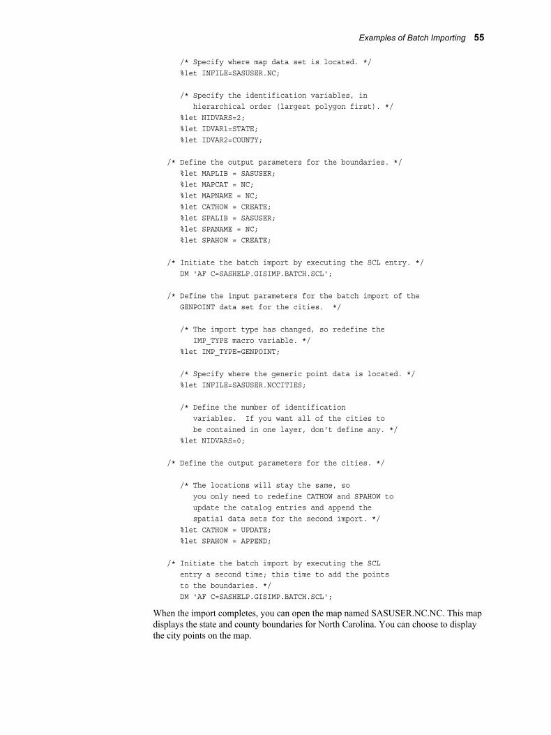
/* Specify where map data set is located. */ %let INFILE=SASUSER.NC;
/* Specify the identification variables, in hierarchical order (largest polygon first). */ %let NIDVARS=2; %let IDVAR1=STATE; %let IDVAR2=COUNTY;
/* Define the output parameters for the boundaries. */ %let MAPLIB = SASUSER; %let MAPCAT = NC; %let MAPNAME = NC; %let CATHOW = CREATE; %let SPALIB = SASUSER; %let SPANAME = NC; %let SPAHOW = CREATE;
/* Initiate the batch import by executing the SCL entry. */ DM 'AF C=SASHELP.GISIMP.BATCH.SCL';
/* Define the input parameters for the batch import of the GENPOINT data set for the cities. */
/* The import type has changed, so redefine the IMP_TYPE macro variable. */ %let IMP_TYPE=GENPOINT;
/* Specify where the generic point data is located. */ %let INFILE=SASUSER.NCCITIES;
/* Define the number of identification variables. If you want all of the cities to be contained in one layer, don't define any. */ %let NIDVARS=0;
/* Define the output parameters for the cities. */
/* The locations will stay the same, so you only need to redefine CATHOW and SPAHOW to update the catalog entries and append the spatial data sets for the second import. */ %let CATHOW = UPDATE; %let SPAHOW = APPEND;
/* Initiate the batch import by executing the SCL entry a second time; this time to add the points to the boundaries. */ DM 'AF C=SASHELP.GISIMP.BATCH.SCL';
When the import completes, you can open the map named SASUSER.NC.NC. This map displays the state and county boundaries for North Carolina. You can choose to display the city points on the map.
Examples of Batch Importing 55

File Reference Table for Batch ImportingTable 4.5 on page 56 lists the reserved filerefs for each of the different import types, a brief description of each file, and whether the fileref is required or optional when using that import type. For example, to import a Digital Line Graph file, you must allocate the file with a fileref of DLGIN.
Note: This information can also be found in the SASHELP.GISIMP data set. See “The SASHELP.GISIMP Data Set” on page 43 for more information.
Table 4.5 File Reference Table for Batch Importing
IMP_TYPE Value Fileref File Description Status
TIGER TIGER1 TIGER basic data record (.rt1 file) Required
TIGER2 TIGER shape coordinate points (.rt2 file) Required
TIGER4 TIGER index to alternate feature names (.rt4 file) Optional
TIGER5 TIGER feature name list (.rt5 file) Optional
TIGER6 TIGER additional address and ZIP code (.rt6 file) Optional
DYNAMAP GDT1 Dynamap basic data record Required
GDT2 Dynamap shape coordinate points Required
GDT4 Dynamap index to alternate feature names Optional
GDT5 Dynamap feature name list Optional
GDT6 Dynamap additional address and ZIP code data Optional
DLG DLGIN Digital Line Graph file Required
DXF DXFIN DXF file Required
ARC ARCIN Uncompressed ArcInfo interchange (E00) file Required
MAPINFO MIF MapInfo Interchange Format MIF file Required
MID MapInfo Interchange Format MID file Required
SASGRAPH and generic import types require that the spatial data be stored in a SAS data set. Therefore, do not allocate a reserved fileref to indicate the location of the data set. Instead, assign the name of the SAS data set to the INFILE macro variable.
56 Chapter 4 • Batch Importing

TIGER 2007 – Present Shapefile Variables for the FACES File Type
FACES type shapefiles contain attribute data for the left and right sides of map features such as Census Tract, Block Group, and Block values. Variable names in FACES type shapefiles change depending on the year the shapefile was created, so the variables read during the import process will change by year as well.
For example, when importing 2007-2009 TIGER/Line shapefiles, state FIPS codes from the STATEFP variable are read. But when importing 2010 TIGER/Line shapefiles, the STATEFP10 values are read from the FACES type shapefile. Documentation available on the U.S. Census Bureau website explains the variables in each TIGER/Line shapefile for a specific release year.
The default FACES variables used are listed below by release year. The table also includes the SAS macro variable in which the FACES variable name is stored. You can override the default FACES variable by defining a different FACES variable name in the appropriate SAS macro variable. In that case, your specified FACES variable will be imported instead of the default.
Note: The FACES type shapefile variables that are imported are printed in the SAS log and in the summary output text file.
Table 4.6 FACES Type Variables Imported by TIGER Release Year
SAS Macro Variable Description 2007–2009 2010 2011–present
STATEVAR State FIPS codes STATEFP STATEFP10 STATEFP10
COUNTYVAR County FIPS codes COUNTYFP COUNTYFP10 COUNTYFP10
TRACTVAR Census Tracts TRACTCE00 TRACTCE10 TRACTCE10
BLKGRPVAR Census Block Groups BLKGRPCE00 BLKGRPCE10 BLKGRPCE10
BLOCKVAR Census Blocks BLOCKCE00 BLOCKCE10 BLOCKCE10
PLACEVAR Census-designated Places
PLACEFP PLACEFP10 PLACEFP
CSAVAR Census Combined Statistical Areas
CSAFP CSAFP10 CSAFP
CBSAVAR Census Core-Based Statistical Areas
CBSAFP CBSAFP10 CBSAFP
METDIVVAR Census Metropolitan Divisions
METDIVFP METDIVFP10 METDIVFP
TIGER 2007 – Present Shapefile Variables for the FACES File Type 57

Hints and Tips for Batch Importing• The SAS/GIS batch import process provides less error checking than the GIS Spatial
Data Importing window. Ensure that the values that you define for the input parameters are valid. Defining invalid values for the input parameters will cause the import to fail.
• The GIS Spatial Data Importing window interface lets you modify the default composites and the default layer definitions before you proceed with the import. The batch import process does not provide this functionality. To modify the composites and layers before the import occurs, you must use the GIS Spatial Data Importing window. However, it does not matter which method you use to complete the import. You can always use PROC GIS after the import is complete to make changes to your map and its underlying components.
• The batch import for the 1990 – 2006 TIGER and DYNAMAP import types does not automatically import all of the files, only the required file types 1 and 2. To use the batch import process to import any or all of the optional file types, you need to perform the following steps:
1. Copy the SASHELP.GISIMP data set to a location where you have Write access. For example, copy the SASHELP.GISIMP data set into the SASUSER library:
proc copy in=sashelp out=sasuser; select gisimp / mt=data;run;
2. Edit the SASUSER.GISIMP data set and change the value of the REQ variable for the TIGER or DYNAMAP file type from 0 (zero) to 1. For example, you have the TIGER4 and TIGER5 filerefs allocated to the TIGER file types 4 and 5, and you want them to be imported. In that case, you could run the following DATA step to change the value of the REQ variable:
data sasuser.gisimp; set sasuser.gisimp; /* Make sure that the values of the FILEREF variable are in all uppercase. */ if fileref in ('TIGER4' 'TIGER5') then req=1;run;
However, you could also use FSBROWSE, FSVIEW, VIEWTABLE, or any other method that you are familiar with to change the value of the REQ variable. Just remember that for the import type that you choose, it will import only from the filerefs for which REQ=1 in the data set.
3. For SAS/GIS to use the new SASUSER.GISIMP data set, you must define the USER_FIL macro variable to point to the name of the new data set. For example:
%let USER_FIL=SASUSER.GISIMP;
As long as the USER_FIL macro variable is defined when the SASHELP.GISIMP.BATCH.SCL entry is executed, it will use the current values of REQ to specify which files are imported.
• The SASHELP.GISIMP data set also contains the default librefs for the output catalog entries and spatial data sets. You can modify these defaults by making a copy of the SASHELP.GISIMP data set and changing the values for the DEFMLIB and
58 Chapter 4 • Batch Importing

DEFSLIB variables to a valid, assigned libref. You then need to define the macro variable USER_FIL to point to your modified copy of the data set.
• The data set that is specified by the USER_FIL macro variable is used by both the batch and interactive imports. Consider the case where you have modified a copy of the SASHELP.GISIMP data set and assigned the data set name to the USER_FIL macro variable. However, you do not want to have that data set used for a specific import. You need to redefine the USER_FIL macro variable to point to the default data set, SASHELP.GISIMP, before performing either an interactive or a batch import.
• Throughout this chapter, all of the macro variable names, their values, and all filerefs have been shown in all uppercase for clarity. However, their names and values are not case-sensitive. For example, the following four statements are equivalent:
%let imp_type=sasgraph;%let imp_type=SASGRAPH;%let IMP_TYPE=sasgraph;%let IMP_TYPE=SASGRAPH;
Hints and Tips for Batch Importing 59

60 Chapter 4 • Batch Importing

Chapter 5
Working with Spatial Data
SAS/GIS Data Sets . . . . . . . . . . . . . . . . . . . . . . . . . . . . . . . . . . . . . . . . . . . . . . . . . . . . 61SAS Data Sets . . . . . . . . . . . . . . . . . . . . . . . . . . . . . . . . . . . . . . . . . . . . . . . . . . . . . . 61Chains Data Set . . . . . . . . . . . . . . . . . . . . . . . . . . . . . . . . . . . . . . . . . . . . . . . . . . . . . 62Nodes Data Set . . . . . . . . . . . . . . . . . . . . . . . . . . . . . . . . . . . . . . . . . . . . . . . . . . . . . 62Details Data Set . . . . . . . . . . . . . . . . . . . . . . . . . . . . . . . . . . . . . . . . . . . . . . . . . . . . 63Polygonal Index Data Sets . . . . . . . . . . . . . . . . . . . . . . . . . . . . . . . . . . . . . . . . . . . . 63Label Data Set . . . . . . . . . . . . . . . . . . . . . . . . . . . . . . . . . . . . . . . . . . . . . . . . . . . . . . 63Attribute Data Sets . . . . . . . . . . . . . . . . . . . . . . . . . . . . . . . . . . . . . . . . . . . . . . . . . . 63Managing Data Set Sizes . . . . . . . . . . . . . . . . . . . . . . . . . . . . . . . . . . . . . . . . . . . . . 63Import Type Specific Variables . . . . . . . . . . . . . . . . . . . . . . . . . . . . . . . . . . . . . . . . 64
Data Set and Catalog Entry Interactions . . . . . . . . . . . . . . . . . . . . . . . . . . . . . . . . . . 69Catalog Entry Types Used by SAS/GIS . . . . . . . . . . . . . . . . . . . . . . . . . . . . . . . . . . 69Spatial Entries . . . . . . . . . . . . . . . . . . . . . . . . . . . . . . . . . . . . . . . . . . . . . . . . . . . . . . 70Coverage Entries . . . . . . . . . . . . . . . . . . . . . . . . . . . . . . . . . . . . . . . . . . . . . . . . . . . . 71Layer Entries . . . . . . . . . . . . . . . . . . . . . . . . . . . . . . . . . . . . . . . . . . . . . . . . . . . . . . . 72Map Entries . . . . . . . . . . . . . . . . . . . . . . . . . . . . . . . . . . . . . . . . . . . . . . . . . . . . . . . . 73Composites . . . . . . . . . . . . . . . . . . . . . . . . . . . . . . . . . . . . . . . . . . . . . . . . . . . . . . . . 73
Merging Spatial Data with the MERGE= Argument . . . . . . . . . . . . . . . . . . . . . . . . 74Overview . . . . . . . . . . . . . . . . . . . . . . . . . . . . . . . . . . . . . . . . . . . . . . . . . . . . . . . . . . 74Types of Merge Operations . . . . . . . . . . . . . . . . . . . . . . . . . . . . . . . . . . . . . . . . . . . 74Benefits of Merging Data . . . . . . . . . . . . . . . . . . . . . . . . . . . . . . . . . . . . . . . . . . . . . 75
Sample SAS/GIS Spatial Database . . . . . . . . . . . . . . . . . . . . . . . . . . . . . . . . . . . . . . . 75
Hints and Tips for Working with Spatial Data . . . . . . . . . . . . . . . . . . . . . . . . . . . . . 75
SAS/GIS Data Sets
SAS Data SetsA SAS data set is a collection of data values and their associated descriptive information. This collection is arranged and presented in a form that can be recognized and processed by SAS. SAS data sets can be data files or views. A SAS data file contains the following elements:
• data values that are organized into a rectangular structure of columns and rows
• descriptor information that identifies attributes of both the data set and the data values
61

A SAS view contains the following elements:
• instructions to build a table
• descriptor information that identifies attributes of both the data set and the data values
SAS data sets can be indexed by one or more variables, known as key variables. A SAS index contains the data values of the key variables that are paired with location identifiers for the observations that contain the variables. The value and identifier pairs are ordered in a B-tree structure that enables the engine to search by value. SAS indexes are classified as simple or composite, according to the number of key variables that they contain.
For more information about SAS data sets, SAS files, SAS views, and SAS indexes, refer to SAS Language Reference: Concepts.
As a component of SAS, SAS/GIS stores all of its data in SAS data sets. The SAS/GIS spatial database works as one logical entity, but is physically separated into six different categories of data sets:
• chains
• nodes
• details
• polygonal index
• label
• attribute
A given SAS/GIS map can reference only one chains, nodes, details, and label data set, but it can reference multiple polygonal index and attribute data sets. Multiple SAS/GIS maps can use a single set of chains, nodes, and details data sets.
Chains Data SetThe chains data set contains coordinates for the polylines that are used to form line and polygon features. A polyline consists of a series of connected line segments that are chains. A chain is a sequence of two or more points in the coordinate space. The end points, the first and last points of the chain, must be nodes. Each chain has a direction, from the first point toward the last point. The first point in the chain is the from-node, and the last point is the o-node. Relative to its direction, a chain has a left side and a right side. Points between the from-node and the to-node are detail points, which serve to trace the curvature of the feature that is represented by the chain. Detail points are not nodes.
The chains data set also lists the from-node and to-node row numbers in the nodes data set. It also lists the number of detail points and the corresponding details data set row number. The left and right side attribute values (for example, ZIP codes and FIPS codes) are also stored in the chains data set.
Nodes Data SetThe nodes data set contains the coordinates of the end points for the chains in the chains data set. It also contains the linkage information that is necessary to attach chains to the correct nodes. A node is a point in the spatial data with connections to one or more chains. Nodes can be discrete points or the end points of chains. A node definition can
62 Chapter 5 • Working with Spatial Data

span multiple records in the nodes data set, so only the starting record number for a node is a node feature ID.
Details Data SetThe details data set stores the curvature points of a chain between the two end nodes, which are also called the from-node and the to-node. That is, the details data set contains all the coordinates between the intersection points of the chain. The node coordinates are not duplicated in the details data set. The details data set also contains the chains data set row number of the associated chain.
Polygonal Index Data SetsThe polygonal index data set contains one observation for each polygon that was successfully closed during the index creation process. It is called a polygonal index because each observation is an index to a polygon in the chains data set. That is, it points to the starting chain in the chains data set for each of the polygons.
If polygon areas, perimeter distances, and centroid locations were computed, then that information is also stored in the polygonal index data set.
Label Data SetThe label data set defines the attributes of labels to be displayed on the map. The attributes include all of the information that is applicable for each label. Information includes location, color, size, source of the text for a text label, as well as other behavioral and graphical attributes.
Attribute Data SetsAttribute data sets contain values related to the map features. The observations in attribute data sets must be associated with observations in the chains data set. Attribute data is used to display themes on the map and for spatially oriented reports, graphs, map actions, and so on.
Managing Data Set SizesBy their nature, spatial databases tend to be rather large. Users of spatial data want as much detail in the maps as they can get, which increases the demands on storage and processing capacity. Spatial data that is not carefully managed can become too large for easy use.
Here are five actions that you can take to manage the size of your spatial data sets. You need to perform most of these actions before importing your data into SAS/GIS.
• Reduce the spatial extent of the data.
Do not store a larger area than you need. If you need a map containing one state, do not store a map containing all the states for a region. For example, if you need to work with a map of Oregon, do not store a map containing all of the Pacific Northwest.
• Store only the features that you need.
If you do not need features such as rivers and lakes, do not store these features in your spatial data.
SAS/GIS Data Sets 63

• Limit the amount of detail to what is necessary for your application.
If you are using a map for which you do not require highly detailed boundaries, reduce the detail level and save storage space. If you are using SAS/GRAPH data sets, you can use the GREDUCE procedure in SAS/GRAPH software to reduce the detail level. If you are using a data set from another source, you must reduce the level of detail before importing the data set into SAS/GIS.
• Reduce the number of attributes that are stored with the spatial data.
If you do not need an attribute, and do not think you will ever need it again, delete it from your spatial data.
• Reduce the size of variables that are stored in the spatial data.
Examine the method that you use for storing your variables and determine whether you can safely reduce the variable size that you use to store them.
For example, you can have a numeric variable that contains a code that can be a maximum of two digits. In this case, it might be better to store it in a two-digit character variable rather than in an eight-byte numeric variable. Change the variables' defined types or lengths in a DATA step after you complete the import.
Of the five actions, reducing the number of attributes is the easiest to perform. Use the Modify Composites window. Access this window by selecting Modify Composites from the GIS Spatial Data Importing window. You can remove and drop unneeded composite variables from your data set as it is imported.
Import Type Specific VariablesThe following tables describe the composites and variables that are created for each of the import types. All of the variables are located in the chains data set except for the X and Y variables, which are in the nodes data set.
In the following table, the values in the Type column represent the following data types:
A Area
C Classification
X X coordinate
Y Y coordinate
Table 5.1 Composites and Variables for SAS/GIS Spatial Data Imported from ArcInfo Interchange Data
Composite Variable 1 Variable 2 Type Description
ARCID ARCIDL ARCIDR A or C ARCID from the ArcInfo coverage. Maps made from line and point coverages do not contain left and right variables.
ARCNUM C ARCNUM from the coverage.
64 Chapter 5 • Working with Spatial Data

Composite Variable 1 Variable 2 Type Description
'COVERAGE'* 'COVERAGE'L 'COVERAGE'R A or C This variable is derived from the input filename. It is the last word preceding the file extension. For example, /local/gisdata/montana.e00 would have a 'COVERAGE' name of montana. The left variable would be montanal, the right variable would be montanar, and the composite type would be Area. Line and point coverages do not have left- and right-side variables, and the composite type would be Classification.
AREA AREAL AREAR A AREA from the coverage.
PERIMETER PERIML PERIMR A PERIMETER from the coverage.
'ATTRIB' 'ATTRIB'L 'ATTRIB'R All variables in the polygon, line, or point attribute tables are saved as composite variables. In the case of the polygon coverages, an L or an R is added to the end of the first five characters of the actual variable name.
_COVER_ _COVEL _COVER A or C This variable contains the name stored in the 'COVERAGE' variable.
_SRC_ _SRCL _SRCR C Contains the string 'ARC'.
X X X X coordinate.
Y Y Y Y coordinate.
* Names in single quotation marks, such as 'COVERAGE' and 'ATTRIB,' are GIS composite names.
In the following table, the values in the Type column represent the following data types:
A Area
C Classification
X X coordinate
Y Y coordinate
SAS/GIS Data Sets 65

Table 5.2 Composites and Variables for SAS/GIS Spatial Data Imported from Digital Line Graph (DLG) Data
Composite Variable 1 Variable 2 Type Description
LMAJOR(n) LMAJOR(n) C Major line attribute code.
LMINOR(n) LMINOR(n) C Minor line attribute code.
NMAJOR(n) NMAJOR(n) C Major node attribute code.
NMINOR(n) NMINOR(n) C Minor node attribute code.
MAJOR(n) AMAJORR(n) AMAJORL(n) A Major area attribute code.
MINOR (n) AMINORL(n) AMINORR(n) A Minor area attribute code.
X X X X coordinate.
Y Y Y Y coordinate
In the following table, the values in the Type column represent the following data types:
A Area
C Classification
Table 5.3 Composites and Variables for SAS/GIS Spatial Data Imported from Drawing Interchange File (DXF) Data
Composite Variable 1 Variable 2 Type Description
'ATTRIB' 'ATTRIB'L 'ATTRIB'R A or C All polygon, line, or point attributes are saved as composite variables. In the case of polygon maps, an L or R is added to the end of the first seven characters of the actual variable name.
In the following table, the values in the Type column represent the following data types:
C Classification
X X coordinate
Y Y coordinate
Table 5.4 Partial Listing of Composites and Variables Specific to the Genline Import Type
Composite Variable 1 Variable 2 Type Description
ID ID C The ID variable from the data set.
'ATTRIB' 'ATTRIB' 'ATTRIB' C Any other variable in the data set is saved as a classification composite.
X X X X coordinate.
Y Y Y Y coordinate.
66 Chapter 5 • Working with Spatial Data
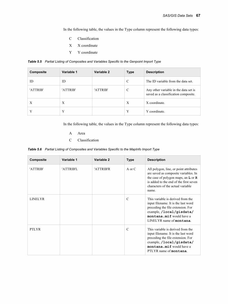
In the following table, the values in the Type column represent the following data types:
C Classification
X X coordinate
Y Y coordinate
Table 5.5 Partial Listing of Composites and Variables Specific to the Genpoint Import Type
Composite Variable 1 Variable 2 Type Description
ID ID C The ID variable from the data set.
'ATTRIB' 'ATTRIB' 'ATTRIB' C Any other variable in the data set is saved as a classification composite.
X X X X coordinate.
Y Y Y Y coordinate.
In the following table, the values in the Type column represent the following data types:
A Area
C Classification
Table 5.6 Partial Listing of Composites and Variables Specific to the MapInfo Import Type
Composite Variable 1 Variable 2 Type Description
'ATTRIB' 'ATTRIB'L 'ATTRIB'R A or C All polygon, line, or point attributes are saved as composite variables. In the case of polygon maps, an L or R is added to the end of the first seven characters of the actual variable name.
LINELYR C This variable is derived from the input filename. It is the last word preceding the file extension. For example, /local/gisdata/montana.mif would have a LINELYR name of montana.
PTLYR C This variable is derived from the input filename. It is the last word preceding the file extension. For example, /local/gisdata/montana.mif would have a PTLYR name of montana.
SAS/GIS Data Sets 67

Composite Variable 1 Variable 2 Type Description
POLYLYR A This variable is derived from the input filename. It is the last word preceding the file extension. For example, /local/gisdata/montana.mif would have a POLYLYR name of montana.
'MAP' 'MAP'L 'MAP'R A or C This variable is derived from the input filename. It is the last word preceding the file extension. For example, /local/gisdata/usa.mif, would have a 'MAP' name of usa. The left variable would be usal, the right variable would be usar and, in this case, the composite type would be Area. Line and point maps do not have left- and right-side variables, and the composite would be Classification.
In the following table, the value in the Type column represents the following data type:
A Area
Table 5.7 Partial Listing of Composites and Variables Specific to the SAS/GRAPH and Genpoly Import Types
Composite Variable 1 Variable 2 Type Description
'IDVAR'n 'IDVAR'L 'IDVAR'R A An area composite variable is created for each ID variable (IDVAR) selected by the user in the ID vars list box. In the case of polygon maps, an L or R is added to the end of the first seven characters of the actual variable name.
In the following table, the values in the Type column represent the following data types:
A Area
ADDR Address
ADDRP Address Prefix
ADDRS Address Suffix
C Classification
X Longitude
Y Latitude
68 Chapter 5 • Working with Spatial Data

Table 5.8 Composites and Variables Specific to the TIGER and DYNAMAP Import Types
Composite Variable 1 Variable 2 Variable 3 Variable 4 Type Description
ADDR FRADDL FRADDR TOADDL TOADDR ADDR Address range.
BLOCK BLOCKL BLOCKR A Block number.
CFCC CFCC C Feature classification code.
COUNTY COUNTYL COUNTYR A County FIPS code.
DIRPRE DIRPRE ADDRP Feature direction prefix.
DIRSUF DIRSUF ADDRS Feature direction suffix.
FEANAME FEANAME C Feature name.
MCD MCDL MCDR A Minor civil division.
PLACE PLACEL PLACER A Incorporated place code.
RECTYPE RECTYPE C Record type.
STATE STATEL STATER A State FIPS code.
TRACT TRACTL TRACTR A Census tract.
ZIP ZIPL ZIPR A ZIP code.
BG BGL BGR A Block group.
LONGITUDE
X X Longitude.
LATITUDE Y Y Latitude.
Data Set and Catalog Entry Interactions
Catalog Entry Types Used by SAS/GISSAS/GIS software uses SAS catalog entries to store metadata for the spatial database, that is, information about the spatial data values in the spatial data sets. SAS/GIS spatial databases use the following entry types:
• spatial entries
• coverage entries
• layer entries
• map entries
• composites
Data Set and Catalog Entry Interactions 69

Spatial Entries
OverviewA spatial entry is a SAS catalog entry of type GISSPA that identifies the spatial data sets for a given spatial database. A spatial entry also defines relationships between the variables in those data sets.
Spatial entries are created and modified using the SPATIAL statement in the GIS procedure.
Note: You can also create a new spatial entry by selecting the following from the GIS Map window's menu bar:File ð Save As ð Spatial
SAS/GIS software supports simple spatial entries and merged spatial entries.
Simple Spatial EntriesSimple spatial entries contain the following elements:
• references to the chains, nodes, and details data sets that contain spatial information.
• references to any polygonal index data sets that define the boundaries of area features in the spatial data.
• definitions for composites that specify how the variables in the spatial data sets are used. See “Composites” on page 73 for more information about composites.
• the definition for a lattice hierarchy that specifies which area features in the spatial data enclose or are enclosed by other features.
• parameters for the projection system that is used to interpret the spatial information that is stored in the spatial data sets.
• the accumulated bounding extents of the spatial data coordinates of its underlying child spatial data sets. This consists of the minimum and maximum X and Y coordinate values and the ranges of X and Y values.
Merged Spatial EntriesMerged spatial entries have the following attributes:
• consist of multiple SAS/GIS spatial databases that are linked together hierarchically in a tree structure.
• contain logical references to two or more child spatial entries. A child spatial entry is a dependent spatial entry beneath the merged spatial entry in the hierarchy.
• contain specifications of how the entries were merged (by overlapping or edge matching).
• do not have their own spatial data sets.
• reference the spatial data sets that belong to the child spatial entries beneath them on the hierarchy.
• do not have references to any polygonal index data sets that define the boundaries of area features in the spatial data.
• do not have definitions for composites that specify how the variables in the spatial data sets are used. See “Composites” on page 73 for more information about composites.
70 Chapter 5 • Working with Spatial Data

• do not have the definition for a lattice hierarchy that specifies which area features in the spatial data enclose or are enclosed by other features.
• do not have parameters for the projection system that is used to interpret the spatial information stored in the spatial data sets.
• contain the accumulated bounding extents of the spatial data coordinates of their underlying child spatial entries. This consists of the minimum and maximum X and Y coordinate values and the ranges of X and Y values.
Merged spatial entries can help you manage your spatial data requirements. For example, you might have two spatial databases that contain the county boundaries of adjoining states. You can build a merged spatial entry that references both states and view a single map that contains both states' counties. Otherwise, you would have to import a new map containing the two states' counties. This new map would double your spatial data storage requirements.
The following additional statements in the GIS procedure update the information in the spatial entry:
COMPOSITE statementcreates or modifies composites that define the relation and function of variables in the spatial data sets. The composite definition is stored in the spatial entry. See “COMPOSITE Statement” on page 101 for details about creating or modifying composites.
POLYGONAL INDEX statementupdates the list of available index names stored in the spatial entry. See “POLYGONAL INDEX Statement” on page 107 for details about creating and modifying polygonal indexes.
LATTICE statementupdates the lattice hierarchy stored in the spatial entry. See “LATTICE Statement” on page 110 for details about defining lattice hierarchies.
You can view a formatted report of the contents of a spatial entry by submitting a SPATIAL CONTENTS statement in the GIS procedure.
See “SPATIAL Statement” on page 96 for details about using the GIS procedure to create, modify, or view the contents of spatial entries.
Coverage EntriesA coverage entry is a SAS catalog entry of type GISCOVER that defines the subset, or coverage, of the spatial data that is available to a map. SAS/GIS maps refer to coverages rather than directly to the spatial data.
A coverage entry contains the following elements:
• a reference to the root spatial entry.
• a WHERE expression that describes the logical subset of the spatial data that is available for display in a map.
Note: The expression WHERE='1' can be used to define a coverage that includes all the data that is in the spatial database. WHERE='1' is called a universal coverage.
The WHERE expression binds the coverage entry to the spatial data sets that it subsets. The WHERE expression is checked for compatibility with the spatial data when the coverage entry is created and also whenever a map that uses the coverage entry is opened.
Data Set and Catalog Entry Interactions 71

• the maximum and minimum X and Y coordinates in the portion of the spatial data that meets the WHERE expression criteria for the coverage.
These maximum and minimum coordinates are evaluated when the coverage is created. The GIS procedure's COVERAGE CREATE statement reads the matching chains and determines the extents from the chains' XMIN, YMIN, XMAX, and YMAX variables. If you make changes to the chains, nodes, and details data sets that affect the coverage extents, use the COVERAGE UPDATE statement to update the bounding extent values.
Multiple coverage entries can refer to the same spatial entry to create different subsets of the spatial data for different maps. For example, you could define a series of coverages to subset a county into multiple sales regions according to the block groups that are contained in each of the regions. The spatial data for the entire county would still be in a single spatial database. The data is represented by the chains, nodes, and details data sets and by the controlling spatial entry.
Coverage entries are created and modified by using the COVERAGE statement in the GIS procedure. You can view a formatted report of the contents of a coverage entry by submitting a COVERAGE CONTENTS statement in the GIS procedure. (The contents report for a coverage entry also includes all the contents information for the root spatial entry as well.)
See “COVERAGE Statement” on page 113 for more information about creating, modifying, or viewing the contents of coverage entries.
Layer EntriesA layer entry is a SAS catalog entry of type GISLAYER that defines the set of features that compose a layer in the map. A layer entry contains the following elements:
• a WHERE expression that describes the common characteristic of features in the layer.
The WHERE expression binds the layer entry to the spatial data even though the WHERE expression is stored in the layer entry. The layer is not bound to a specific spatial entry, just to those entries that represent the same type of data. Therefore, a layer that is created for use with data that is imported from a TIGER file can be used with data that is imported from any TIGER file. However, not all file types can take advantage of this behavior. The WHERE expression is checked for compatibility with spatial data when the layer entry is created and also whenever a map that uses the layer entry is opened.
Note: When you define area layers, you can specify a composite as an alternative to specifying an explicit WHERE expression. However, the layer entry stores the WHERE expression that is implied by the composite. For example, if you specify STATE as the defining composite for a layer, and the STATE composite specifies the following variables: VAR=(LEFT=STATEL,RIGHT=STATER), then the implied WHERE expression that is stored in the layer entry is 'STATEL NE STATER'.
• option settings for the layer. Settings can include the layer type (point, line, or area), or whether the layer is static or thematic. Other settings indicate whether the layer is initially displayed or hidden, or whether detail points are drawn for the layer. Still other settings specify the scales at which the layer is automatically turned on or off.
• the graphical attributes that are necessary to draw the layer when it is displayed as a static layer.
72 Chapter 5 • Working with Spatial Data

• the attribute links, theme range breaks, and graphical attributes if the layer contains themes.
See “LAYER Statement” on page 116 for more information about creating, modifying, or viewing the contents of layer entries.
Map EntriesA map entry is a SAS catalog entry of type GISMAP. Map entries are the controlling entries for SAS/GIS maps because they tie together all the information that is needed to display a map. A map entry contains the following elements:
• a reference to the coverage entry that defines the subset of the spatial data that is available to the map. Note that the map entry refers to a particular coverage of the spatial data rather than directly to the spatial entry.
• references to the layer entries for all layers that are included in the map.
• references to any attribute data sets that are associated with the map. For example, the data sets that are used for the map actions, along with definitions of how the attribute data sets are linked to the spatial data.
• a reference to the SAS data set that contains labels for map features.
• definitions for the actions that can be performed.
• definitions for map legends.
• parameters for the projection system that is used to project the spatial data coordinates for display.
• option settings for the map, including the following:
• the units and mode for the map scale
• whether coordinate, distance, and attribute feedback are displayed
• whether detail points are read
• whether the tool palette is active
Map entries are created by using the MAP CREATE statement in the GIS procedure. However, much of the information that is stored in the map entry is specified interactively in the GIS Map window.
You can view a formatted report of the contents of a map entry by submitting a MAP CONTENTS statement in the GIS procedure. (The contents report for a map entry includes all the contents information for the spatial, coverage, and layer entries as well.) See “MAP Statement” on page 142 for details about using the MAP statement. See Chapter 10, “ SAS/GIS Windows” in SAS/GIS Software: Usage and Reference, Version 6, for details about the items that can be specified interactively in the GIS Map window.
CompositesFor most operations that involve the spatial database, you refer to composites of the spatial data variables rather than directly to the variables in the spatial data sets. A composite consists of the following elements:
• a variable association that identifies which variable or variables in the spatial database comprise the association. The variable association can specify a single variable, or a pair of variables that define a bilateral (left-right) association. The association can also specify two pairs of variables that define the start and end of a directional (from-to) bilateral association.
Data Set and Catalog Entry Interactions 73

• a class attribute that identifies the role of the composite in the spatial database.
For example, if the chains data set has a variable named FEANAME that contains feature names. You can create a composite for the FEANAME variable. The composite assigns the class attribute NAME to indicate that it represents feature names. In another example, the chains data set has COUNTYL and COUNTYR variables that contain the codes for the counties on the left and right sides of the chains. You can create a composite named COUNTY. The composite identifies the bilateral relationship between these two variables and assigns the class attribute AREA to indicate that the association defines county areas in the spatial data.
Composites are created and modified using the COMPOSITE statement in the GIS procedure. Composite definitions are stored in the spatial entry. When a spatial action is performed in a map, the variables referenced by composites for the selected map features are displayed in the Spatial Information window. See “COMPOSITE Statement” on page 101 for more information about creating or modifying composites.
Merging Spatial Data with the MERGE= Argument
OverviewMERGE= is an argument of the GIS procedure's SPATIAL statement that enables you to build a new spatial entry by referencing two or more existing spatial entries. The dependent data sets for the spatial entries are not actually combined when you use the MERGE= argument; the new spatial entry includes them by reference. For more information about the syntax for the MERGE= option, see “SPATIAL Statement” on page 96.
Note: Keep in mind that MERGE is specified as an option in a SPATIAL statement.
If you specify a one-level name for any of the entries to be merged, the spatial entry is assumed to be in one of two catalogs. It will be the catalog that is specified either in the CATALOG= argument with the PROC GIS statement or in the most recently issued CATALOG statement. An error occurs if you have not specified a catalog before specifying the names of the entries that you want to merge.
Types of Merge OperationsThe MERGE= argument accepts the following arguments:
EDGEMATCHlocates common boundaries between the merged spatial entries and updates missing left- or right-side composite variable values in the chains data that lie on the boundaries.
In other words, the EDGEMATCH operation compares the chains in the different data sets and finds those chains that map the same feature. First it finds the same chain in both data sets. Then it identifies any missing left- or right-side composite values in either chain. It replaces these missing values with the valid values from the other data set. EDGEMATCH also creates a merged spatial entry that references other spatial entries (either merged or simple) that you specified with the MERGE= argument.
EDGEMATCH rewrites the specified chains data sets. You cannot reverse this operation.
74 Chapter 5 • Working with Spatial Data

OVERLAPmerges spatial entries without attempting to match boundaries. OVERLAP is the default behavior of the MERGE= argument. The OVERLAP argument creates a merged spatial entry that references the specified spatial entries (either merged or simple).
OVERLAP does not rewrite the specified chains data sets.
For more information, see “SPATIAL Statement” on page 96.
Benefits of Merging DataMerging data enables you to construct maps that show larger geographic areas without the overhead of storing duplicate spatial data sets. For example, you might have chains, nodes, and details data sets for each U.S. state. If you want to create a map of New England, you do not have to physically combine and duplicate the individual data sets for the six states composing the region. Instead, you can create a merged spatial entry named New_England that references the individual states' simple spatial entries.
Edge matching provides a mechanism to update adjoining spatial data sets to replace missing left or right values in the chains data sets. Let us use the New England example. There are chains in the chains data set for New Hampshire that lie along the Vermont border. These chains contain the FIPS code of 33 on one side of each chain. The other side of each chain has a missing value. The corresponding chains in the Vermont chains data set contain the Vermont FIPS code of 50 on one side and a missing value on the other side. An edge match merge of the two data sets locates these common boundary chains in each data set. It replaces the missing values with the correct FIPS code for the adjoining state. It will also create a merged spatial entry that references the New Hampshire and Vermont simple spatial entries.
The EDGEMATCH operation creates a single merged spatial entry by which you can create a map of the two states. It also adds the Vermont FIPS code to the appropriate chains in the New Hampshire data set. In addition, it adds the New Hampshire FIPS code to the corresponding chains in the Vermont data set.
Sample SAS/GIS Spatial DatabaseSAS/GIS offers a code sample that creates a fully functional SAS/GIS spatial database. This sample is available in the online Help. In the GIS Map window, select Help ð Getting Started with SAS/GIS Software ð Create Data. You can use this sample map with the SAS/GIS interface and the GIS procedure.
Hints and Tips for Working with Spatial Data• When SAS/GIS uses a coverage that is not universal—that is, one in which the value
of the WHERE expression is not '1'—to subset a map, all of the layers in the map must also satisfy this WHERE expression. If any of the layers do not satisfy this WHERE expression, some features of the map might not be displayed, and the reason might not be apparent.
For example, suppose you have a map of the United States and you want to create a subset map containing just North Carolina and Virginia. You can use the following COVERAGE statement to create the subset map:
Hints and Tips for Working with Spatial Data 75

COVERAGE CREATE NCVA / where='STATEL IN(37 51) OR STATER IN(37 51)';
Any points or lines that do not have 37 or 51 as the STATEL or STATER value are not to be displayed on the map.
• Defining a layer with WHERE='1' displays all of the features in the underlying spatial data that have that type. For example, you can have a map with a point layer that contains capital cities. Then you add a new point layer for grocery store locations by using WHERE='1' for the layer definition. The grocery store layer will display all of the point features in the spatial data. This layer includes capital cities, grocery stores, and all other point features in the spatial data. You might find this confusing if you are not aware that all point features are being displayed when you intend to display only one layer.
You might encounter this situation because the GENPOINT import, by default, defines all point layers with a WHERE='1' expression. You can click the Modify layers button on the GIS Spatial Data Importing window to redefine the layer definition. Change it to a WHERE expression that uniquely identifies the set of points in the layer. If the layer already exists on the map, you can use the LAYER statement in the GIS procedure to redefine the layer. Use a WHERE expression that defines only those points in the layer.
76 Chapter 5 • Working with Spatial Data

Chapter 6
Batch Geocoding
Overview of Batch Geocoding . . . . . . . . . . . . . . . . . . . . . . . . . . . . . . . . . . . . . . . . . . . 77
Addresses in Spatial Data . . . . . . . . . . . . . . . . . . . . . . . . . . . . . . . . . . . . . . . . . . . . . . 78
Using Batch Geocoding . . . . . . . . . . . . . . . . . . . . . . . . . . . . . . . . . . . . . . . . . . . . . . . . 79
How Batch Geocoding Works . . . . . . . . . . . . . . . . . . . . . . . . . . . . . . . . . . . . . . . . . . . 79Data Requirements for Geocoding . . . . . . . . . . . . . . . . . . . . . . . . . . . . . . . . . . . . . . 79Created Data Sets . . . . . . . . . . . . . . . . . . . . . . . . . . . . . . . . . . . . . . . . . . . . . . . . . . . 79Reference Data Sets . . . . . . . . . . . . . . . . . . . . . . . . . . . . . . . . . . . . . . . . . . . . . . . . . 80Match Addresses . . . . . . . . . . . . . . . . . . . . . . . . . . . . . . . . . . . . . . . . . . . . . . . . . . . . 80Address Match Scoring . . . . . . . . . . . . . . . . . . . . . . . . . . . . . . . . . . . . . . . . . . . . . . . 81
%GCBATCH Macro Statement . . . . . . . . . . . . . . . . . . . . . . . . . . . . . . . . . . . . . . . . . 83
Batch Geocoding Example . . . . . . . . . . . . . . . . . . . . . . . . . . . . . . . . . . . . . . . . . . . . . . 85Example Code . . . . . . . . . . . . . . . . . . . . . . . . . . . . . . . . . . . . . . . . . . . . . . . . . . . . . . 85Example Results . . . . . . . . . . . . . . . . . . . . . . . . . . . . . . . . . . . . . . . . . . . . . . . . . . . . 87
Hints and Tips for Batch Geocoding . . . . . . . . . . . . . . . . . . . . . . . . . . . . . . . . . . . . . . 88
Overview of Batch GeocodingGeocoding is the process of adding location information to an existing data set that contains address data. SAS/GIS software provides a facility for batch geocoding of address data sets.
Note: The SAS/GIS batch geocoder has been superseded by the GEOCODE procedure. For more information, see “GEOCODE Procedure” in SAS/GRAPH: Reference.
The SAS/GIS geocoding facility attempts to match each address in a SAS address data set to a location on a map. Location information is the X and Y coordinate data for the street addresses. If a match is found, the X and Y coordinates of the address are added to the address data set. Other attribute information about the matched location can also be added to the address data set.
SAS/GIS software provides an interactive interface for geocoding through the GIS Geocoding window. The window is convenient for geocoding individual address data sets. However, the batch geocoding facility is useful for geocoding a large number of data sets or a data set with a large number of observations. The batch geocoding facility in SAS/GIS allows data to be geocoded without invoking SAS/GIS, without user intervention, and with improved performance. For example, you can set up a program to run overnight to geocode address data sets without user interaction.
77

Addresses in Spatial DataIn order to use geocoding in SAS/GIS, your spatial database must contain address information. SAS/GIS uses CLASS values for composites to identify address information in the spatial database. One of the composites must be defined as CLASS=CITY to indicate the city name, and one of the composites must be defined as CLASS=ADDRESS to indicate the location portion of the address. Composites that are defined with other CLASS values, such as ZIP, serve to improve accuracy. You use the COMPOSITE CREATE statement in the GIS procedure to add address-related composites to the spatial entry. You can use the SPATIAL CONTENTS statement in the GIS procedure to view the composites that are defined for your spatial database.
The following composite CLASS values identify elements of the address information:
NAMEidentifies the name component of the address feature, such as Main in the address 101 N Main Ave.
TYPEidentifies the type component of the address feature, such as Ave in the address 101 N Main Ave.
ADDRESSidentifies the specific address of the feature, such as 101 in the address 101 N Main Ave. This composite is required when doing geocoding.
A chain has four values to define the address range for each side:
FROMLEFTbeginning address on the left side.
TOLEFTending address on the left side.
FROMRIGHTbeginning address on the right side.
TORIGHTending address on the right side.
DIRECTION_PREFIXidentifies the directional prefix component of the address feature, such as N in the address 101 N Main Ave.
DIRECTION_SUFFIXidentifies the directional suffix component of the address feature, such as W in the address 1141 First St W.
CITY | PLACEidentifies the value as a city name. This composite is required when doing geocoding.
STATEidentifies the value as a state name.
ZIPidentifies the value as a ZIP code value.
PLUS4identifies the value as a ZIP+4 extended postal code value.
78 Chapter 6 • Batch Geocoding

You can use the SPATIAL CONTENTS statement in the GIS procedure to determine whether your spatial database contains the minimum composites that are necessary to perform geocoding. Submit the following statements in the SAS Program Editor for the spatial entry that you want to geocode against:
proc gis catalog=libref.catalog;spatial contents spatial-entry;run;quit;
The output that is produced by the SPATIAL CONTENTS statement will include a list of all of the composites that are defined for the specified spatial entry. If the spatial database includes address information, this list will include some or all of the composites that are defined with the required CLASS values for address information.
Using Batch GeocodingUsing the batch geocoding facility is a two-step process:
1. Use the %GCBATCH macro to assign values to the macro variables that control the geocoding process. See “%GCBATCH Macro Statement” on page 83 for more information.
2. Call the SCL program to perform batch geocoding, SASHELP.GIS.GEOCODEB.SCL. In a SAS program, you can use the DM statement to issue an AF command to execute the SCL, as follows:
dm 'af c=sashelp.gis.geocodeb.scl; run;';
Note: If you are invoking SCL from your own frame application, you must use CALL DISPLAY instead of the DM command, for example, call display('sashelp.gis.geocodeb.scl').
How Batch Geocoding Works
Data Requirements for GeocodingTo achieve the most accurate geocoding, ensure that the address data set to be geocoded contains name, address, city, state, ZIP code, and ZIP+4 variables. At least the address and city variables are required.
Created Data SetsThe geocoding facility first reads the chains, nodes, and details data sets for the map specified in the %GCBATCH macro. Then it creates new data sets for the sorted and summarized versions in the SAS library that was specified with the GLIB macro variable. Names for the geocoding data sets are generated from the specified map's chains data set name. For example, if your chains data set is GMAPS.USAC and you specify GLIB=GEOLIB in the %GCBATCH macro, then the geocoding facility creates the following data sets:
How Batch Geocoding Works 79

GEOLIB.USAScontains sorted chains.
GEOLIB.USAMcontains matchable street data summarized from the chains data set and sorted by state, ZIP code, street name, and city.
GEOLIB.USAPcontains point coordinates along the street segment taken from the map's nodes and details data sets.
These summary data sets are created automatically before the first address-matching process begins. After the data sets are created, they are regenerated only when the map's chains data set is updated or when NEWDATA=YES is specified in the %GCBATCH macro.
When choosing the SAS library to use for these created data sets, consider that—depending on the area of the base map—they can be quite large. If you use the WORK library, then the data sets will be deleted at the end of the current SAS session. The data sets must be regenerated if you want to perform geocoding again in a future SAS session.
Reference Data SetsAdditional data sets used in geocoding are supplied by SAS:
SASHELP.GCTYPEcontains the official street abbreviations used by the U.S. Postal Service and in TIGER data from the U.S. Census Bureau. These values are used to standardize your address observations before geocoding.
SASHELP.PLFISPcontains place names, state codes, and FIPS place codes for U.S. locations. The places primarily represent cities and towns, but the data set also includes some national parks, industrial parks, military installations, and so on.
SASHELP.ZIPCODEcontains U.S. ZIP codes, FIPS state and city codes, city names, and post office names. The ata set also contains the latitude and longitude for the centroid of each ZIP code area. If an address is not matched in the primary geocoding data sets, this data set is searched for a matching ZIP code. Updates for this data are available from the SAS Maps Online website http://www.sas.com/mapsonline.
Match AddressesThe geocoding facility uses these data sets to match the addresses in the address data set. As it is processing the address data set, the geocoding facility provides a progress indicator. For every 10% of the addresses that are geocoded, a message is written to the SAS log.
When a match is found, the coordinates of the address location are added to the address data set, along with any other composite values for the specified address. Take, for example, a spatial data that has a composite named TRACT that contains census tract numbers. You can use the geocoding process to add a TRACT variable to your address data set. The resulting geocoded address data set can be used as attribute data for the map. Or it can be imported to add point data to the map by using a generic import.
Sometimes an address cannot be matched to the spatial data but the address includes a ZIP code. In this case the X and Y coordinates of the center of the ZIP code centroid for
80 Chapter 6 • Batch Geocoding

the zone are returned instead of the exact coordinates of the address. The centroid coordinates are read from the SASHELP.ZIPCODE data set.
For matching purposes, the geocoding process converts the address components to uppercase and attempts to convert direction and street type values to standard forms. The standardized versions of the address components are also added to the address data set. The M_ADDR, M_CITY, M_STATE, M_ZIP, and M_ZIP4 variables that are added to the address data set reflect the address values that were actually matched during the geocoding process. If a matching observation was found in the sorted chains data set, that row number is placed in the M_OBS variable.
Address Match ScoringAll address matches are not equal. The geocoding process attempts to match different elements of each specified address. When multiple address elements match, the resulting X/Y location is more certain. The geocoding process adds _SCORE_, _STATUS_, and _NOTES_ variables to the address data set to indicate which elements were matched. These variable values can also indicate whether there was a problem with a specific part of the address.
The _SCORE_ variable's value is a numeric rating of the certainty of the address match. A higher score indicates a better match. The score is calculated by adding points for matching various components of the address.
A score of 100 indicates that a match was found for all of the components of the address. A score of 100 is possible only if the address in the data set includes values for all components and the geocoding lookup data contains variables for all components. For example, the address in the data set does not have a ZIP+4 value or the lookup data set does not have a PLUS4 type variable. In this case the highest possible score is 95.
Table 6.1 _SCORE_ Values for Address Elements
Address Element Matched Value added to _SCORE_ Value
Street number 40
Street name 20
Street type 5
Street direction 5
City 5
State 5
Five-digit ZIP code 15
First three digits of ZIP code 5
ZIP+4 code 5
The _STATUS_ variable provides a general indication of the match result:
How Batch Geocoding Works 81

Table 6.2 _STATUS_ Values for Match Results
_STATUS_ Value Description
found Street name and ZIP code or city and state match found.
X/Y interpolated along street.
_SCORE_ indicates how many elements were matched.
ZIP Match Street name not found in lookup data.
ZIP code was found in SASHELP.ZIPCODE.
X/Y for ZIP center is within the lookup data extents.
ZIP Match OffMap Street name not found in lookup data.
ZIP code was found in SASHELP.ZIPCODE.
X/Y for ZIP center is outside lookup data extents.
City/State Match Street name not found in lookup data.
City and state elements found in SASHELP.ZIPCODE.
Multiple city and state matches were averaged for X/Y.
City not found Address had missing ZIP code value.
City is not in SASHELP.ZIPCODE.
X/Y values are missing.
Unknown Address No part of address was matched.
X/Y values are missing.
The _NOTES_ variable provides additional details about which address elements were matched or invalid:
Table 6.3 _NOTES_ Values for Match Results
_NOTES_ Value Description
ZC Five-digit ZIP code matched.
ZC3 First three digits of ZIP code matched.
AD Street name matched.
TY Street type matched.
DP Street direction prefix matched.
DS Street direction suffix matched.
NM House number matched.
ST State matched.
82 Chapter 6 • Batch Geocoding

_NOTES_ Value Description
CT City matched.
CT3 Used with ZC3. Street matched only first 3-digits of the ZIP code in lookup data. Either the city value was missing in the address or the city and state pair in lookup data differed.
NOADD Street address is invalid.
NOZC Address ZIP code is missing.
NOCT Address city name is invalid.
%GCBATCH Macro StatementThe %GCBATCH macro sets the input parameters for the batch geocoding program. The macro accepts the following information:
• the name of the address data set to geocode
• the variable names in the address data set
• the name of the map entry
• the library in which to store geocoding data sets, and whether new copies of the data sets are created
• the name of an alternate ZIP code centroids data set that is used instead of SASHELP.ZIPCODE
• the names of any additional polygonal composites to add to the address data set
The %GCBATCH macro has the following general form. The elements within the %GCBATCH macro can appear in any order, but they must be separated by commas.
%GCBATCH(<GLIB=geocoding-library,><ZIPD=ZIP-centroids-data-set,>GEOD=address-data-set,<NV=name-var,>AV=address-var,CV=city-var,<SV=state-var,><ZV=ZIP-var,><P4V=ZIP+4-var,>MNAME=map-entry,<PV=area-composite-list,><NEWDATA=YES | NO> );
where
%GCBATCH Macro Statement 83

AV=address-varspecifies the name of the variable that stores the complete street address in the address data set that you want to geocode. This includes the house number, street name, and street type (for example, 3922 Oak Avenue). This parameter is required.
CV=city-varspecifies the name of the variable that stores the city name portion of the address in the address data set that you want to geocode. This parameter is required.
GEOD=address-data-setspecifies the address data set that you want to geocode. This parameter is required.
GLIB=geocoding-libraryspecifies the libref for the SAS library where all of the sorted and summarized chains, nodes, and details data sets that are created for the geocoding process are stored. This parameter is optional.
Note: The SAS library that you specify for the GLIB= argument should be on a volume that has a large amount of free space. The reason is that the geocoding data sets might be quite large. Also, to take full advantage of the geocoding facility, you should specify a permanent SAS library. The default for this variable is WORK, but data sets in the WORK library are deleted when the SAS session is terminated, so the geocoding data sets are lost. Geocoding data sets can already exist in the specified library at the start of the geocoding process. In this case the geocoding facility checks their creation dates against the creation date of the chains data set. The geocoding data sets are created again only if the chains data set has a more recent creation date. The first time you geocode with a particular chains data set, the process takes considerably longer because these geocoding data sets are being created, sorted, and indexed. Subsequent geocoding times, however, are much faster as long as the parent chains data set has not been modified.
MNAME=map-entryspecifies the name of the GISMAP entry for the SAS/GIS spatial database (the chains, nodes, and details data sets) that you are using for geocoding. The map entry contains projection information that the geocoding process uses. The process ensures that the X and Y coordinates that are returned for the address will be in the same coordinate system as the spatial data for the map. The MNAME= argument should use the form libref.catalog-name.entry-name. This parameter is required.
NEWDATA=YES | NOspecifies whether the geocoding lookup data sets are created again if they already exist. The default is NEWDATA=NO. If you set NEWDATA=NO, the geocoding facility searches the SAS library that you specified with the GLIB macro variable for geocode data sets that were created for the spatial entry. The geocoding facility checks the creation date of existing geocode data sets against the creation date of the spatial entry. If the creation date of the geocode data sets is more recent than the creation dates of the spatial entry, the geocoding facility uses the geocode data sets. Otherwise, it creates new geocode data sets.
Use NEWDATA=YES to force the geocoding facility to build new versions of the geocoding data sets. You should specify NEWDATA=YES if the existing geocoding data sets were created with an earlier version of SAS/GIS software. This parameter is optional.
NV=name-varspecifies the name of the variable that stores the name portion of the address in the address data set that you want to geocode.
This parameter is optional.
84 Chapter 6 • Batch Geocoding

PV=area-composite-listspecifies the list of polygonal (area) composite values that you want added as variables to the address data set along with the X and Y coordinates of the address. By default, no other variables are added. Use spaces to separate composite names in the list. For example, the following specification adds the county and census tract and block values along with the address coordinates:pv=county tract block, This parameter is optional.
P4V=ZIP+4-varspecifies the name of the variable that stores ZIP+4 postal codes in the address data set that you want to geocode.
This parameter is not required, but the accuracy of the geocoding process might be reduced if you omit it.
SV=state-varspecifies the name of the variable that stores the state or province name portion of the address in the address data set you want to geocode.
This parameter is not required, but the accuracy of the geocoding process might be reduced if you omit it.
ZIPD=ZIP-centroids-data-setspecifies a data set that contains the coordinates of the centers of ZIP code zones. (If an address includes a ZIP code and the street address cannot be matched, the geocoding facility supplies the ZIP code centroid coordinate instead of the address coordinate.) The default is ZIPD=SASHELP.ZIPCODE, which specifies the SASHELP.ZIPCODE data set that is supplied with SAS software. Updated data sets are available from the SAS Maps Online website http://www.sas.com/mapsonline. This parameter is optional.
ZV=ZIP-varspecifies the name of the variable that stores the ZIP code portion of the address in the address data set that you want to geocode.
This parameter is not required, but the accuracy of the geocoding process might be reduced if you omit it.
Batch Geocoding Example
Example CodeThe following example uses the batch geocoding macro to geocode an address data set using a copy of the MAPS.WAKE.TRACT map supplied with SAS/GIS software. That map was originally created by importing the U.S. Census Bureau TIGER files for Wake County, North Carolina. This example uses a copy in the WORK library rather than the original in either the MAPS or MAPSSAS library. This shows how the geocoded addresses can be imported and appended to the spatial data.
/*--- Copy the base map to the WORK library ---*/proc gis; copy MAPS.WAKE.TRACT.GISMAP / /* Map entry to copy */ destlib = WORK /* Destination library */ destcat = WORK.WAKE /* Destination catalog */ sel = (_all_) /* Copy all map components */ blank /* Clear internal map path */
Batch Geocoding Example 85

replace; /* Overwrite existing entry */quit;
/*--- Create the address data set to geocode ---*/data WORK.ADDRESSES (label='Data set to geocode'); input address $ 1-23 /* Street address */ resident $ 24-48 /* Person at the location */ zip $ 49-53 /* 5-digit US postal code */ city $ 55-69 /* City name */ state $ 70-71; /* US state name */cards;700 Madison Avenue Patricia Smith 27513 Cary506 Reedy Creek Road Jean Francois Dumas 27513 Cary1106 Medlin Drive Michael Garriss 27511 NC1150 Maynard Road Kaspar Gutman 27511 Cary138 Dry Ave. Susan Lang 27511 NC3112 Banks Road Roy Hobbs 27603 Raleigh NC305 Mill Creek Drive Alan Picard 27526 Fuquay-Varina NC1998 S. Main St. Guillermo Ugarte Wake Forest7825 Old Middlesex Rd Capt. Jeffrey Spaulding 27807 Bailey NC5550 Old Stage Road Emily Joyner 27603 Raleigh NC3212 Avent Ferry Road Fred C. Dobbs 27540 NC1050 King Charles Rd. Karin Schmidt . Raleigh NC6819 Buffaloe Road Ferdinand Paulin 27604 NC3211 Constant Circle Gordon Miller 341216111 Old Faison Road Alan Picard 27545 Knightdale725 N. Raleigh Street Evan Rudde 27501 Angier NC;run;
/*--- Set up variables for the Batch Geocoding program ---*/%gcbatch( glib = WORK, /* Geocoding library */ geod = WORK.ADDRESSES, /* Address data to geocode */ nv = RESIDENT, /* Who's at the address */ av = ADDRESS, /* Address variable */ cv = CITY, /* Place name */ sv = STATE, /* State name */ zv = ZIP, /* ZIP code (5-digit) */ pv = TRACT, /* AREA value from map data */ mname = WORK.WAKE.TRACT); /* Map data used for geocoding */
/*--- Run the Batch Geocoding program ---*/dm 'af cat=SASHELP.GIS.GEOCODEB.SCL';
/*--- Show geocoding results on a bar chart -------------------*/axis1 label=(height=1.3 'Address Status');axis2 label=(angle=-90 rotate=90 height=1.3 'Percent');title1 "Geocoding Results";title2 "Wake County, NC";footnote1 j=l "Geocoded by SAS/GIS";proc gchart data=WORK.ADDRESSES; /* Geocoded data set */ vbar _status_ / /* Midpoint (x-axis) variable */ descending /* Order of results */ type = pct /* Response (y-axis) variable */ outside = pct /* Label on top of bars */ inside = freq /* Label inside of bars */
86 Chapter 6 • Batch Geocoding

maxis = axis1 /* x-axis */ raxis = axis2; /* y-axis */ run;quit;
/*--- Set up Batch Import variables ---*/%let imp_type = GENPOINT; /* Importing data as points */%let maplib = WORK; /* Map library */%let mapcat = WAKE; /* Map catalog */%let mapname = TRACT; /* Map catalog entry */%let spalib = WORK; /* Spatial data library */%let spaname = WAKE; /* Spatial entry name */%let cathow = UPDATE; /* Append existing entry */%let spahow = APPEND; /* Append to spatial data sets */%let nidvars = 0; /* Put points in one layer */%let infile = WORK.ADDRESSES; /* Data set to import */
/*--- Run the Batch Import program ---*/DM 'af cat=SASHELP.GISIMP.BATCH.SCL';
/*--- Modify imported layer and map with GIS Procedure ---*/proc gis cat=WORK.WAKE; /*--- Set display parmameters for imported point layer */ layer update ADDRESSES / /* Geocoded layer */ type = point /* Layer type */ where = 'node=1' /* Layer definition */ des = 'Geocoded addresses' /* Label for entry */ default = (point=(color = yellow /* Symbol color */ font = marker /* Symbol font */ character = 'V' /* Symbol to use */ size = 10)); /* Symbol height */ /*--- Set display parmameters for the map */ map update TRACT / /* Map entry name */ layerson = (TRACT ADDRESSES) /* Turn on layers */ cback = gray /* Background color */ legend = hideall /* Turn off legend */ des = 'Wake County geocoding'; /* Label for entry */ /*--- Add label in lower right corner of the map */ maplabel create / text = 'Geocoding by SAS/GIS' /* Label text */ map = WORK.WAKE.TRACT /* Map entry */ attach_to = window /* Do not pan label */ position = (bottom right) /* Window position */ color = cxA81010; /* Text color */ run;quit;
/*--- Open map in SAS/GIS ---*/dm 'gis map=WORK.WAKE.TRACT';
Example ResultsThe geocoded latitude and longitude values are written to the WORK.ADDRESSES input data set, along with the census tract values for each found address. The match results for each geocoded address are also written to that data set. A bar chart that
Batch Geocoding Example 87

summarizes the results of the geocoding process is generated using the GCHART procedure in SAS/GRAPH software.
When the import is complete, the map opens in SAS/GIS. The found locations are in the map's ADDRESSES point layer.
Note: The WHERE clause for the ADDRESSES point layer is WHERE='NODE=1', which displays points for all of the found addresses. You can modify the WHERE clause to show only those addresses that were matched with a higher degree of certainty (for example,.WHERE='_SCORE_>=40').
Note: For a more detailed example of batch geocoding, see the article “Cheap Geocoding: SAS/GIS and TIGER Data,” available in the Geocoding section of the Downloads page in the SAS Maps Online website http://www.sas.com/mapsonline. The article is a reprint of a presentation from SAS Global Forum 30. The article is also available in the proceedings for that conference.
Hints and Tips for Batch Geocoding• To ensure good quality and accurate geocoding results, you must use accurate data.
If your map's address data is incomplete or out of date, your geocoding will not deliver the results that you want.
• You can import the geocoded addresses onto a map. However, before you import the points, you must make sure that your address data set contains a variable named ID that has a unique value for each point.
• The input address data set contains the addresses that you want to geocode. This data set should contain variables for the street address, city, state, and ZIP code (and an optional ZIP+4 code) of the addresses to be matched. The address data set can also contain a name that is associated with the address, but the name is not used in the address matching. In order for the geocoding facility to most accurately parse the addresses, follow these guidelines:
• Use only street addresses. Post office boxes, rural routes, grid addresses, and addresses with alphanumeric characters cannot be geocoded. An address containing a post office box or a rural route address in addition to a street address should not cause a problem.
• The street number portion of the street address should not contain non-numeric characters. For example, an address such as 501-B Kent St will be matched to 501 Kent St., not to the full address containing the non-numeric character. Apartment numbers should be stored in separate variables rather than appended to the street number.
• Use the following values for directional prefixes and suffixes, with no punctuation or spaces between letters:
N S E W NE NW SE SW
• Avoid using abbreviations that conflict with street name abbreviations. For example, do not use St John St. Use Saint John St instead. Spelling out Saint reduces chances for confusion.
Note: The results from the geocoding are written back to the address data set, so you must have Write access to it or make a copy that you can write to.
88 Chapter 6 • Batch Geocoding

• You can create your own geocoding lookup data sets for specific areas of the United States by downloading and importing TIGER data from the U.S. Census Bureau. See “Importing Spatial Data” on page 25 for more information.
You can also download ready-to-use geocoding lookup data sets for the entire United States from the SAS Maps Online website http://www.sas.com/mapsonline. After downloading and installing these data sets, you can use them to geocode any U.S. address.
Hints and Tips for Batch Geocoding 89

90 Chapter 6 • Batch Geocoding

Chapter 7
The GIS Procedure
Overview: GIS Procedure . . . . . . . . . . . . . . . . . . . . . . . . . . . . . . . . . . . . . . . . . . . . . . 91
Concepts: GIS Procedure . . . . . . . . . . . . . . . . . . . . . . . . . . . . . . . . . . . . . . . . . . . . . . . 92How GIS Procedure Statements Are Processed . . . . . . . . . . . . . . . . . . . . . . . . . . . . 92Data Set Names in the GIS Procedure . . . . . . . . . . . . . . . . . . . . . . . . . . . . . . . . . . . 93Catalog Entry Names in the GIS Procedure . . . . . . . . . . . . . . . . . . . . . . . . . . . . . . . 93
Syntax: The GIS Procedure . . . . . . . . . . . . . . . . . . . . . . . . . . . . . . . . . . . . . . . . . . . . . 94PROC GIS Statement . . . . . . . . . . . . . . . . . . . . . . . . . . . . . . . . . . . . . . . . . . . . . . . . 94CATALOG Statement . . . . . . . . . . . . . . . . . . . . . . . . . . . . . . . . . . . . . . . . . . . . . . . 95SPATIAL Statement . . . . . . . . . . . . . . . . . . . . . . . . . . . . . . . . . . . . . . . . . . . . . . . . . 96COMPOSITE Statement . . . . . . . . . . . . . . . . . . . . . . . . . . . . . . . . . . . . . . . . . . . . . 101POLYGONAL INDEX Statement . . . . . . . . . . . . . . . . . . . . . . . . . . . . . . . . . . . . . 107LATTICE Statement . . . . . . . . . . . . . . . . . . . . . . . . . . . . . . . . . . . . . . . . . . . . . . . . 110COVERAGE Statement . . . . . . . . . . . . . . . . . . . . . . . . . . . . . . . . . . . . . . . . . . . . . 113LAYER Statement . . . . . . . . . . . . . . . . . . . . . . . . . . . . . . . . . . . . . . . . . . . . . . . . . 116LAYERLABEL Statement . . . . . . . . . . . . . . . . . . . . . . . . . . . . . . . . . . . . . . . . . . . 134MAP Statement . . . . . . . . . . . . . . . . . . . . . . . . . . . . . . . . . . . . . . . . . . . . . . . . . . . . 142MAPLABEL Statement . . . . . . . . . . . . . . . . . . . . . . . . . . . . . . . . . . . . . . . . . . . . . 156COPY Statement . . . . . . . . . . . . . . . . . . . . . . . . . . . . . . . . . . . . . . . . . . . . . . . . . . . 164MOVE Statement . . . . . . . . . . . . . . . . . . . . . . . . . . . . . . . . . . . . . . . . . . . . . . . . . . 166SYNC Statement . . . . . . . . . . . . . . . . . . . . . . . . . . . . . . . . . . . . . . . . . . . . . . . . . . . 168
Overview: GIS ProcedureThe GIS procedure creates and maintains the spatial databases that are used by SAS/GIS software. A SAS/GIS spatial database consists of the following elements:
• SAS data sets that contain the coordinates and identifying information for the spatial features.
• a spatial entry (a SAS catalog entry of type GISSPA) that identifies which SAS data sets contain spatial information. The spatial entry also stores the following elements:
• composites that define how the variables in the spatial data are used
• names of the polygonal indexes that define the boundaries of area layers for the map
• a lattice hierarchy that defines which features in the spatial data enclose or are enclosed by other features (the relationships among the polygonal variables)
• information about the projection method that is used for the stored spatial data
91

A spatial entry alternatively can contain references to two or more other spatial entries that have been merged into a single spatial database.
• a coverage entry (a SAS catalog entry of type GISCOVER) that selects a subset of the spatial data that is available for display in a map.
• one or more layer entries (SAS catalog entries of type GISLAYER) that identify features that have common characteristics and specify how they are displayed as layers in the map.
• a map entry (a SAS catalog entry of type GISMAP) that specifies which layers from a particular coverage are included in a map. The map entry also stores the following information:
• the names of attribute data sets that are associated with the map, along with definitions of how the attribute data is linked to the spatial data
• the name of a SAS data set that contains labels for map features
• definitions of GIS actions that can be performed when map features are selected
• definitions for map legends
• values for display and projection options
Note: The task of creating new SAS/GIS spatial databases from spatial data in other formats can also be performed interactively. Use the GIS Spatial Data Importing window or programmatically use the SAS/GIS batch import process.
Concepts: GIS Procedure
How GIS Procedure Statements Are ProcessedThe GIS procedure supports RUN-group processing. RUN-group processing enables you to invoke the procedure and then submit additional procedure statements without submitting the PROC statement again.
In other SAS procedures that do not support RUN-group processing, a RUN statement that follows a block of submitted statements terminates the procedure. With RUN-group processing, a RUN statement executes the preceding block of statements, but the procedure remains active. You can continue to submit additional statements for the active procedure without resubmitting the PROC statement. For example, the following code invokes the GIS procedure, assigns a default catalog, and identifies the current spatial entry:
proc gis catalog=mymaps.region; spatial norwest;
Note: The SPATIAL, CATALOG, LATTICE, COPY, MOVE, and SYNC statements are immediate statements for the GIS procedure. That is, they are always processed immediately and do not require a RUN statement (although including a RUN statement does not do any harm).
After you invoke the GIS procedure, suppose that you also want to define composites. You can submit additional GIS procedure statements to define the composites without submitting a new PROC statement, as shown in the following example:
composite create state / class=state
92 Chapter 7 • The GIS Procedure

var=(left=statel,right=stater);composite create county / class=area var=(left=countyl,right=countyr); composite create lat / class=y var=y; composite create lon / class=x var=x;run;
You can end RUN-group processing and terminate the GIS procedure by submitting a QUIT statement:
quit;
Submitting another PROC step, a DATA step, or an ENDSAS statement also ends RUN-group processing and terminates the GIS procedure.
Note: Certain error conditions might also terminate the GIS procedure. If this occurs, a message is printed in the SAS log.
Data Set Names in the GIS ProcedureYou can specify a data set by its complete two-level name as in libref.data-set. If you omit the libref value, the data set is assumed to be in the library specified in the CATALOG= option in the PROC GIS statement or in the catalog that was specified by the most recent CATALOG statement.
Note: If a one-level catalog name was used in the CATALOG= option or CATALOG statement, or if no default catalog has been named, the default library is WORK (for example, WORK).data-set.
Catalog Entry Names in the GIS ProcedureYou can specify a GIS catalog entry by its complete three-level name, libref.catalog.entry-name. If you use only the one-level entry-name value, the entry is assumed to be in the catalog that is specified in the CATALOG= option in the PROC GIS statement or in the catalog specified by the most recent CATALOG statement.
Note: If the libref value was omitted from the CATALOG= option or catalog statement, the default library is WORK. If no default catalog has been declared, and a one-level entry-name value is used, then an error is written to the log because of insufficient information to identify the entry.
Concepts: GIS Procedure 93

Syntax: The GIS ProcedurePROC GIS <CATALOG=<libref.>catalog>;
CATALOG <libref.>catalog;SPATIAL <operation> <libref.catalog.>spatial-entry </ options>;COMPOSITE operation composite-name </ options>;POLYGONAL INDEX operation polygonal-index </ options>;LATTICE outer-composite-name-1 ENCLOSES inner-composite-name-1
<… outer-composite-name-n ENCLOSES inner-composite-name-n><_UNIVERSE_ ENCLOSES inner-composite-name>;
COVERAGE operation <libref.catalog.>coverage-entry </ options>;LAYER operation <libref.catalog.>layer-entry </ options>;LAYERLABEL operation <options>;MAP operation <libref.catalog.>map-entry </ options>;MAPLABEL<operation> <option>COPY <libref.catalog.>entry-name<.type> </ options> ;MOVE <libref.catalog.>entry-name<.type> </ options>;SYNC <libref.catalog.>entry-name<.type> </ options>;
PROC GIS StatementInvokes the GIS procedure and specifies the default SAS catalog in which the spatial, coverage, layer, and map entries are stored.
SyntaxPROC GIS <CATALOG=<libref.>catalog-name>;
Optional ArgumentCATALOG=<libref.>catalog-name
specifies the default SAS catalog in which the GIS spatial, coverage, layer, and map entries referred to in subsequent statements in the PROC GIS step are stored. If the specified catalog does not already exist, it is created when a subsequent SPATIAL, COVERAGE, LAYER, or MAP statement is executed.
Aliases CAT=
C=
Default If you omit the libref value in the argument, the default SAS library, WORK, is used.
DetailsThe CATALOG= argument is overridden when you perform one of the following:
94 Chapter 7 • The GIS Procedure

• issue a CATALOG statement in conjunction with the PROC GIS statement. Subsequent statements in the GIS procedure will refer to the catalog that was named in the most recent CATALOG statement. It will not refer to the one that is specified in the CATALOG= option in the PROC GIS statement.
• specify fully qualified (three-level) entry names in SPATIAL, COVERAGE, LAYER, or MAP statements. This temporarily overrides the default catalog for the current statement only. It does not reset any catalog that is specified with the CATALOG= option. See the descriptions of these statements for more information.
CATALOG StatementIdentifies the default SAS catalog in which GIS spatial, coverage, layer, and map entries are stored when you specify one-level catalog entry names in subsequent statements in the PROC step.
Note: The CATALOG statement permanently replaces the CATALOG= option that is specified in the PROC GIS statement. If you use the CATALOG= option in the PROC GIS statement and then submit a CATALOG statement, subsequent statements in the GIS procedure refer to the catalog that was named in the most recent CATALOG statement.
SyntaxCATALOG <CONTENTS <options>> <libref.>catalog-name;
Required Argument<libref.>catalog-name
specifies the name of the catalog that is used in CREATE, REPLACE, and UPDATE operations in subsequent statements. If the specified catalog does not already exist, it is created when a subsequent SPATIAL, COVERAGE, LAYER, or MAP statement is executed.
Default If you do not specify a libref, the WORK library is used.
OperationCONTENTS <options>
displays information about the entries in the specified catalog to the SAS Output window. The CONTENTS operation takes the following options:
ET = (entry-type-list)specifies the catalog entry types to display. The entry-type-list value can contain any combination of MAP, SPATIAL, COVERAGE, and LAYER.
STATEMENTdisplays PROC GIS statements that create the specified entries.
VERBOSElists all information about the catalog (type of map, layers, actions, and associated data sets).
CATALOG Statement 95

DetailsYou can temporarily override the CATALOG statement by specifying fully qualified (three-level) entry names in the SPATIAL, COVERAGE, LAYER, and MAP statements. This does not reset the current default catalog.
SPATIAL StatementSelects the spatial entry on which subsequent statements operate and displays information about the contents of a spatial entry. Also, creates a new spatial entry, replaces an existing spatial entry, modifies the characteristics of an existing spatial entry, or deletes a spatial entry.
SyntaxSPATIAL <operation> <libref.catalog.>spatial-entry </ options>;
Summary of Optional Arguments
CARTESIAN | LATLONspecifies the coordinate system that is used in the stored spatial data.
CHAINS=data-setnames the SAS data set that contains chain definitions for the spatial database.
DEGREES | RADIANS | SECONDSspecifies the coordinate units for the stored spatial data when the coordinate system is geographic.
DESCRIPTION='string'specifies a descriptive phrase that is stored in the description field of the spatial entry.
DETAILS=data-setnames the SAS data set that contains detail definitions for the spatial database.
EAST | WESTspecifies the hemisphere in which the spatial data points lie.
KEEPspecifies that polygonal index data sets are not deleted when the spatial entry is deleted.
MERGE=(spatial-entry-list) <EDGEMATCH <LINKONLY> | OVERLAP <ZEROMISS>> <ERROR_ROW=integer>
builds a new spatial entry by referencing two or more existing spatial entries.MULT=multiplier-value
specifies a constant value by which the stored spatial data coordinates are multiplied.
NODES=data-setnames the SAS data set that contains node definitions for the spatial database.
NORTH | SOUTHindicates the hemisphere in which the spatial data points lie.
96 Chapter 7 • The GIS Procedure
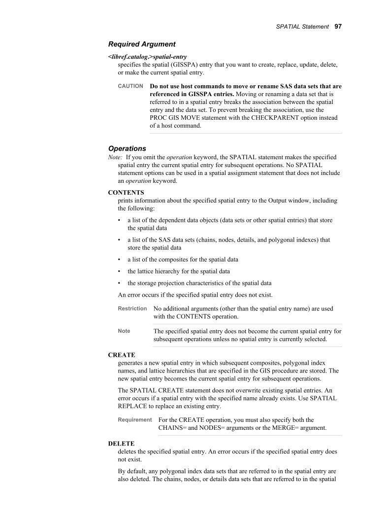
Required Argument<libref.catalog.>spatial-entry
specifies the spatial (GISSPA) entry that you want to create, replace, update, delete, or make the current spatial entry.
CAUTION Do not use host commands to move or rename SAS data sets that are referenced in GISSPA entries. Moving or renaming a data set that is referred to in a spatial entry breaks the association between the spatial entry and the data set. To prevent breaking the association, use the PROC GIS MOVE statement with the CHECKPARENT option instead of a host command.
OperationsNote: If you omit the operation keyword, the SPATIAL statement makes the specified
spatial entry the current spatial entry for subsequent operations. No SPATIAL statement options can be used in a spatial assignment statement that does not include an operation keyword.
CONTENTSprints information about the specified spatial entry to the Output window, including the following:
• a list of the dependent data objects (data sets or other spatial entries) that store the spatial data
• a list of the SAS data sets (chains, nodes, details, and polygonal indexes) that store the spatial data
• a list of the composites for the spatial data
• the lattice hierarchy for the spatial data
• the storage projection characteristics of the spatial data
An error occurs if the specified spatial entry does not exist.
Restriction No additional arguments (other than the spatial entry name) are used with the CONTENTS operation.
Note The specified spatial entry does not become the current spatial entry for subsequent operations unless no spatial entry is currently selected.
CREATEgenerates a new spatial entry in which subsequent composites, polygonal index names, and lattice hierarchies that are specified in the GIS procedure are stored. The new spatial entry becomes the current spatial entry for subsequent operations.
The SPATIAL CREATE statement does not overwrite existing spatial entries. An error occurs if a spatial entry with the specified name already exists. Use SPATIAL REPLACE to replace an existing entry.
Requirement For the CREATE operation, you must also specify both the CHAINS= and NODES= arguments or the MERGE= argument.
DELETEdeletes the specified spatial entry. An error occurs if the specified spatial entry does not exist.
By default, any polygonal index data sets that are referred to in the spatial entry are also deleted. The chains, nodes, or details data sets that are referred to in the spatial
SPATIAL Statement 97

entry are not deleted. To retain existing polygonal index data sets when the spatial entry is deleted, use the KEEP argument in the SPATIAL DELETE statement.
Restriction KEEP is the only additional argument (other than the spatial entry name) that can be used with the DELETE operation.
Note For the DELETE operation, you can also specify the special value _ALL_ for the spatial entry name argument to delete all spatial entries in the current catalog.
CAUTION Use the DELETE operation with care. The GIS procedure does not prompt you to verify the request before deleting the spatial entry. Be especially careful when you use the _ALL_ keyword.
REPLACEoverwrites the specified spatial entry or creates a new entry if an entry with the specified name does not exist. The specified spatial entry becomes the current spatial entry for subsequent operations. The SPATIAL REPLACE statement has the effect of canceling all previously issued SPATIAL CREATE, COMPOSITE, POLYGONAL INDEX, and LATTICE statements for the specified spatial entry.
Requirement For the REPLACE operation, you must specify both the CHAINS= and NODES= arguments or the MERGE= argument.
UPDATEmodifies the specified spatial entry by applying new values for specified arguments. The updated spatial entry becomes the current spatial entry for the subsequent operations.
An error occurs if there is no existing spatial entry with the specified name.
OptionsWhen you specify CREATE, REPLACE, or UPDATE for the operation argument, you can specify one or more of the following additional optional arguments. When you specify DELETE for the operation argument, only the KEEP option is allowed. Separate the list of arguments from the spatial entry name with a slash (/).
CARTESIAN | LATLONspecifies the coordinate system that is used in the stored spatial data.
CARTESIANdata is in an arbitrary rectangular (plane) coordinate system.
LATLONdata is in a geographic (spherical) coordinate system.
Default LATLON
Interaction The CARTESIAN and LATLON arguments are ignored when the MERGE= argument is used.
CHAINS=data-setnames the SAS data set that contains chain definitions for the spatial database. A chain is one or more line segments that connect one node (or point on the map) to another. For example, a series of chains can represent a railroad or a river.
Note The CHAINS= argument is required when you use the CREATE or REPLACE keyword and do not specify the MERGE= argument.
98 Chapter 7 • The GIS Procedure

DEGREES | RADIANS | SECONDSspecifies the coordinate units for the stored spatial data when the coordinate system is geographic (LATLON).
Default RADIANS
Interaction This argument is ignored when the CARTESIAN or MERGE= arguments are used.
DESCRIPTION='string'specifies a descriptive phrase, up to 256 characters long, that is stored in the description field of the spatial entry.
Default The default description is blank.
DETAILS=data-setnames the SAS data set that contains detail definitions for the spatial database. The endpoints of a chain are nodes. Details are the intermediate points along a chain between the nodes that delineate angle breaks in chains. They provide a finer granularity for the chain's line segments. A data set that contains detail definitions might describe the curvy outline of a coastal road.
EAST | WESTspecifies the hemisphere in which the spatial data points lie. EAST refers to points east of the Prime Meridian (0 degrees longitude) at Greenwich, England. WEST refers to points west of the Prime Meridian.
If your data is in the Western Hemisphere, longitude values (the X coordinates) are negative, that is -35° 45' 08”. If your data is in the Western Hemisphere but has positive longitudes, your map is displayed flipped or with the east and west directions reversed. See “Preparing Spatial Data” on page 11 for an example of this behavior. Applying the WEST argument to the spatial data causes the longitudes to be negated when the data is read in, and the map is displayed correctly.
Default EAST
Interaction This argument is ignored when the CARTESIAN or MERGE= arguments are used.
KEEPspecifies that polygonal index data sets are not deleted when the spatial entry is deleted.
Restriction This option is valid only with the DELETE operation.
MERGE=(spatial-entry-list) <EDGEMATCH <LINKONLY> | OVERLAP <ZEROMISS>> <ERROR_ROW=integer>
builds a new spatial entry by referencing two or more existing spatial entries. The dependent data sets for the spatial entries are not actually combined when you use the MERGE argument; the new spatial entry includes them by reference. An error occurs if any of the specified spatial entries do not exist.
You can specify any of the following additional arguments in conjunction with the MERGE= argument:
EDGEMATCH <LINKONLY>matches common boundaries between the merged spatial entries. Missing values along common boundary chains are filled in where possible by using values from
SPATIAL Statement 99

the adjoining spatial data sets. The affected chains data sets are rewritten unless the LINKONLY option is specified, and you cannot reverse the operation.
ZEROMISSINGtreats any left/right attribute value of zero as a missing value. Otherwise, zero is considered to be a valid value when performing an EDGEMATCH merge.
ERROR_ROW=integerprints an enhanced error message for the specified spatial data row during an EDGEMATCH merge operation. This option can be useful for determining what caused a specific row to fail to merge. The basic log warning will print the row number for unmatched chains in all of the merged data sets. Any of these chain numbers can be used as the ERRORROW= target.
OVERLAPmerges spatial entries without attempting to match boundaries. The chains data sets for the merged entries are not rewritten.
Default OVERLAP
MULT=multiplier-valuespecifies a constant value by which the stored spatial data coordinates are multiplied.
Default 1
Interaction This argument is ignored when the MERGE= argument is used.
NODES=data-setnames the SAS data set that contains node definitions for the spatial database. Nodes are the endpoints of map chains. A node can also be a single map feature represented by a point. A single node can be the endpoint for multiple chains, as at a street intersection.
Note The NODES= argument is required when you use the CREATE or REPLACE keyword and do not specify the MERGE= argument.
NORTH | SOUTHindicates the hemisphere in which the spatial data points lie. If your data is in the southern hemisphere (below the equator), latitude values (the Y coordinates) are negative (for example, -45° 12' 33”). If your data is in the southern hemisphere, but the latitude values are positive, your map is displayed inverted with the north and south directions reversed. Applying the SOUTH argument to the spatial data causes the latitude values to be negated when the data is read in. The map is displayed with the correct side up.
Default NORTH
Interaction This argument is ignored when the CARTESIAN or MERGE= arguments are used.
DetailsA spatial entry is a SAS catalog entry of type GISSPA that defines the components of a SAS/GIS spatial database. The definition specifies which SAS data sets contain spatial information, how the data sets are related, and what roles the variables play.
Any composites, polygonal indexes, and lattice hierarchies that are created or updated during an invocation of the GIS procedure are stored in the current spatial entry. Any
100 Chapter 7 • The GIS Procedure

subsequent COVERAGE statements that are issued within the PROC GIS step subset the data in the current spatial entry.
No additional arguments (other than the spatial entry name) are used when the operation keyword is omitted. An error occurs if there is no existing spatial entry that has the specified name.
Note: When creating or replacing spatial entries, you can either define entirely new spatial entries or merge two or more existing spatial entries.
Examples
Example 1: Define the Current Spatial EntryThe following code fragment makes MAPS.NC.NC.GISSPA the current spatial entry that is used for subsequent operations:
proc gis cat=maps.nc; spatial nc;
Example 2: Update an Existing Spatial EntryThe following code fragment replaces the existing details data set with MAPS.USAD for the existing MAPS.USA.USA.GISSPA spatial entry:
spatial update maps.usa.usa / details=maps.usad;
Example 3: Merge Three Existing Spatial DatabasesThe following code fragment creates a new spatial entry that is named TRIANGLE.GISSPA in the current catalog by merging three existing spatial entries, ORANGE, DURHAM, and WAKE. In this example, each of the spatial entries to be merged is stored in a different library. See “Working with Spatial Data” on page 61 for more information about merging.
spatial create triangle / merge=(gmap1.orange.orange, gmap2.durham.durham, gmap3.wake.wake);
COMPOSITE StatementDefines, modifies, or deletes associations between variables in the chains and nodes data sets.
SyntaxCOMPOSITE operation composite-name </ options>;
Summary of Optional Arguments
BILATERALindicates that the composite is a left/right type for spatial data variables that apply to the left and right sides of chains.
CLASS=class-typedefines the role of the composite in the spatial database.
VAR=association-declaration
COMPOSITE Statement 101

defines a variable or an association between related variables in the current spatial chains or nodes data set.
Required Argumentcomposite-name
specifies the composite that you want to create, replace, delete, or update. The composite-name value must conform to the following rules for SAS names:
• The name can be no more than 32 characters long.
• The first character must be a letter or underscore (_). Subsequent characters can be letters, numeric digits, or underscores. Blanks are not permitted.
• Mixed-case names are honored for presentation purposes. However, because any comparison of names is not case sensitive, you cannot have two names that differ only in case (for example, State and STATE are read as the same name).
OperationsYou must specify one of the following values for the operation keyword:
CREATEdefines associations between variables in the chains and nodes data sets and stores these composites in the current spatial entry. The COMPOSITE CREATE statement does not overwrite existing composites. A warning is issued and processing of the current RUN group is halted if a composite with the specified name already exists. Use COMPOSITE REPLACE to overwrite an existing composite.
Note Not all spatial database variables are composites of multiple SAS data set variables. Some composites represent a single SAS data set variable.
DELETEdeletes the specified composite from the current spatial entry. For the DELETE operation, you can also specify the following alternative forms for the composite-name argument:
• a list of composite names, separated by spaces, to delete more than one composite in a single DELETE operation
• the special value _ALL_ to delete all the composites in the current spatial entry
A warning is issued and processing of the current RUN group is halted if the specified composite does not exist.
Restriction No additional arguments (other than the composite name) are used with the DELETE operation.
Note The DELETE operation of the COMPOSITE statement removes a composite from the spatial entry but does not delete the SAS variables from their respective SAS data sets.
CAUTION Use DELETE with care. The GIS procedure does not prompt you to verify the request before deleting an existing composite. Be especially careful when you use _ALL_.
REPLACEoverwrites the previous definition of a composite in the current spatial entry, or creates a new composite if the specified composite-name value did not previously exist.
102 Chapter 7 • The GIS Procedure

UPDATEapplies new values for the specified arguments to an existing composite. A warning is issued and processing of the current RUN group is halted if there is no existing composite with the specified name.
OptionsWhen you specify CREATE, REPLACE, or UPDATE for the operation argument in a COMPOSITE statement, you can specify one or more of the following additional optional arguments. Separate the list of options from the composite-name value with a slash (/).
BILATERALindicates that the composite is a left/right type for spatial data variables that apply to the left and right sides of chains. BILATERAL composites are used to define polygonal layers in a LAYER statement by denoting chains that have different left and right values. This argument provides an implicit VAR= argument, where the LEFT= and RIGHT= variable names are constructed by appending L and R to the specified composite name. For example, the following two statements are equivalent:
composite create state / class=area bilateral;
composite create state / class=area var=(left=statel,right=stater);
CLASS=class-typedefines the role of the composite in the spatial database. The CLASS= option links specific functionality to particular composites.
The class-type value for the CLASS= option can be one of the following:
ADDRESSindicates that the composite defines addresses in the chains data set that is used for geocoding.
Data set address values are the numeric portion of a street address (for example, the 100 in the street address, 100 North Main Street). A chain has four values to define the address range for each side:
FROMLEFTbeginning address on the left side.
TOLEFTending address on the left side.
FROMRIGHTbeginning address on the right side.
TORIGHTending address on the right side.
When you use specify ADDRESS for the class-type value, you must use the following form of the VAR= argument:
VAR=(<FROMLEFT=>variable, <FROMRIGHT=>variable,<TOLEFT=>variable, <TORIGHT=>variable)
AREAindicates that the composite defines polygonal areas.
For polygonal areas that represent political subdivisions, you can specify the following alternative class-type values to indicate which features the areas represent:
COMPOSITE Statement 103

COUNTRYindicates that the composite defines countries in the chains data.
COUNTYindicates that the composite defines counties in the chains data.
STATEindicates that the composite defines states in the chains data. Composites of this class are used in geocoding.
When you use AREA (or COUNTRY, STATE, or COUNTY) for the class-type value, you must specify the bilateral form of the VAR= argument to specify the variables that identify the features on the left and right sides of each chain in the area:
VAR=(<LEFT=>variable, <RIGHT=>variable)
CITY | PLACEindicates that the composite defines features that are related to geographic location, such as cities. Composites of this class are used in geocoding.
By default, CITY is not considered an AREA-type composite. If your spatial data contain closed city boundaries, you must explicitly define the composite as an AREA class as well:
composite create towns / var=(cityl cityr) class=(city area);
CLASSIFICATIONindicates that the composite defines a general descriptive value that can be used to classify features in the map.
Note When you add points to the map interactively in the GIS Map window, you can create new point layers. To enable this creation, you must define at least one CLASSIFICATION-type composite in the spatial entry.
DIRECTION_PREFIXindicates that the composite defines the directional prefix component of an aggregate feature name, such as the North in North Main Ave. Composites of this class are used in geocoding.
DIRECTION_SUFFIXindicates that the composite defines the direction suffix component of an aggregate feature name, such as the South in 2nd St South. Composites of this class are used in geocoding.
NAMEindicates that the composite defines the names of features in the chains data, such as Central Park, or the name component of an aggregate feature name, such as the Main in E Main St. Composites of this class are used in geocoding.
PLUS4indicates that the composite defines extended postal delivery codes (U.S. ZIP+4) in the chains data. Composites of this class are used in address matching.
By default, PLUS4 is not considered an AREA-type composite. If your chains data contain closed ZIP+4 boundaries, you must explicitly define the composite as an AREA class as well:
composite create zip4 / var=(zip4l zip4r) class=(area plus4);
104 Chapter 7 • The GIS Procedure

TYPEindicates that the composite defines the feature type component of an aggregate feature name, such as the Ave in N Harrison Ave. Composites of this class are used in geocoding.
Xindicates that the composite defines the X coordinates for the nodes in the nodes data set.
Yindicates that the composite defines the Y coordinates for the nodes in the nodes data set.
ZIPCODEindicates that the composite defines postal delivery codes in the chains data. Composites of this class are used in geocoding.
By default, ZIPCODE is not considered an AREA-type composite. If your chains data set contains closed ZIP code area boundaries, you must explicitly define the composite as an AREA class as well:
composite create zip / var=(zipl zipr) class=(zipcode area);
Default CLASSIFICATION
VAR=association-declarationdefines a variable or an association between related variables in the current spatial chains or nodes data set. Variables for all composites are assumed to be in the chains data set except for CLASS=X and CLASS=Y variables, which must be in the nodes data set.
The VAR= argument is required when you use the CREATE or REPLACE operations, except in the following circumstances:
• If you omit the VAR= argument and specify CLASS=CLASSIFICATION (or omit the CLASS= argument), the composite-name value that you specify is also used as the variable name. For example, the following statements are equivalent:
composite create cfcc;
composite create cfcc / var=cfcc class=classification;
• If you omit the VAR= argument and specify one of the bilateral class-type values such as AREA or STATE, the suffixes L and R are added to the composite-name value to form the variable name pair for the association. For example, the following statements are equivalent:
composite create state / class=state;
composite create state / class=state var=(statel stater);
For other class-type values, the VAR= argument is required when you use the CREATE or REPLACE keywords.
The association-declaration argument for the VAR= option can be one of the following, depending on the class-type values that are specified in the CLASS= option:
COMPOSITE Statement 105

variabledeclares a composite consisting of a single SAS variable. Use this form for single-variable association classes such as CLASSIFICATION, DIRECTION_PREFIX, DIRECTION_SUFFIX, NAME, TYPE, X, and Y.
(<LEFT=>variable-1, <RIGHT=>variable-2)declares a composite consisting of two variables that represent the left and right sides of a feature. Association declarations of this form can be used to define the boundaries between elements in the spatial data. Use this form for bilateral association classes such as AREA, CITY, COUNTRY, COUNTY, PLACE, STATE, ZIPCODE, and PLUS4.
(<FROMLEFT=>variable-1, <FROMRIGHT=>variable-2, <TOLEFT=>variable-3, <TORIGHT=>variable-4)
declares a composite that consists of four variables that separately represent the beginning and end of the left and right sides of a feature. Association declarations of this form can be used to define the locations of specific addresses in the spatial data. Use this form for the ADDRESS class.
Note: Variable is the name of a SAS data set variable in the chains data set. An error occurs if any of the specified variables do not exist in the chains data set.
DetailsOnce defined, composites can be referenced by other GIS procedure statements. For example, a spatial database can contain the variables COUNTYL and COUNTYR that identify the chains' left and right values for a county ID variable. You could use the COMPOSITE statement to create a composite called COUNTY by associating the two spatial database variables. The COUNTY composite could then be used to define the county boundaries for the map.
Composites are stored in the currently specified spatial (GISSPA) entry. An error occurs if you submit a COMPOSITE statement when no spatial entry is currently selected.
Note: Use the SPATIAL CONTENTS statement to view the composites for a spatial entry. Composite variable values are also displayed in the Spatial Information window when you select a map feature in the GIS Map window.
Examples
Example 1: Define a Single-Variable CompositeThe following code fragment associates the class Y with the variable named LAT in the nodes data set to indicate that the variable contains north-south coordinate information:
composite create latitude / var=LAT class=y;run;
Example 2: Define a Composite for a Bilateral FeatureBoth of the following code fragments associates a pair of variables in the chains data set that contain values for the left and right sides of area boundaries:
composite create state / var=(left=statel,right=stater) class=area;run;
composite create state/ bilateral class=area;
106 Chapter 7 • The GIS Procedure

run;
Example 3: Define a Composite for an Address FeatureThe following code fragment associates two pairs of variables in the chains data set that contain values for the corners of address boundaries:
composite create custadd / var=(fromleft=FRADDL,fromright=FRADDR, toleft=TOADDL,toright=TOADDR) class=address;run;
POLYGONAL INDEX StatementCreates, replaces, modifies, or deletes polygonal index data sets by using a libref and polygonal index references from a spatial entry.
SyntaxPOLYGONAL INDEX operation polygonal-index </ options>;
Summary of Optional Arguments
AREAcalculates the enclosed areas and perimeter lengths for the lowest-level area composite that is specified on the COMPOSITE= argument.
CENTROID<=GEOMETRIC | VISUAL>specifies the type of centroid data that is returned.
COMPOSITE=(composite-name-1<, …, composite-name-n>)specifies the composite or list of composites that define the boundaries of the enclosed polygonal areas that are used to create the index.
ERRORS<=number>specifies whether messages about any topological errors that are detected while the index is being constructed are written to the SAS log.
FORCEindicates that an existing polygonal index data set that is specified in the OUT= argument can be overwritten.
KEEPspecifies that polygonal index data sets are to be retained when the index definition is removed from the spatial entry.
OUT=data-set-namenames the index data set that you want to create, replace, or update.
Required Argumentpolygonal-index
specifies the polygonal index that you want to create, delete, replace, or update. The polygonal-index value must conform to the following rules for SAS names:
• The name can be no more than 32 characters long.
POLYGONAL INDEX Statement 107

• The first character must be a letter or underscore (_). Subsequent characters can be letters, numeric digits, or underscores. Blanks are not permitted.
• Mixed-case names are honored for presentation purposes. However, because any comparison of names is not case sensitive, you cannot have two names that differ only in case (for example, State and STATE are read as the same name).
OperationsYou must specify one of the following values for the operation keyword:
CREATEcreates a polygonal index data set and stores the polygonal index definition in the current spatial entry. The POLYGONAL INDEX CREATE statement does not overwrite existing index definitions or data sets. A warning is issued and processing of the current RUN group is halted if either a polygonal index definition or a SAS data set with the specified names already exist. Use POLYGONAL INDEX REPLACE to replace an existing index definition or data set.
Requirement For the CREATE operation, you must specify both the COMPOSITE= and OUT= arguments.
DELETEremoves the specified polygonal index definition from the spatial entry. By default, the POLYGONAL INDEX DELETE statement also deletes the associated index data set. You can use the KEEP option to prevent the index data set from being deleted.
A warning is issued and processing of the current RUN group is halted if the specified polygonal index does not exist.
For DELETE, you can also specify the special value _ALL_ for the polygonal-index argument to delete all the polygonal index definitions in the current spatial entry.
Restriction KEEP is the only additional argument (other than the polygonal index name) that can be used with the DELETE operation.
CAUTION Use DELETE with care. The GIS procedure does not prompt you to verify the request before deleting an existing polygonal index. Be especially careful when you use the _ALL_.
REPLACEoverwrites the polygonal index definition in the current spatial entry or creates a new polygonal index definition if the specified index does not exist.
Requirement For the REPLACE operation, you must specify both the COMPOSITE= and OUT= arguments.
Note The data set that is specified in the OUT= argument can already exist and belong to a different spatial entry. In this case you must specify the FORCE argument to cause the spatial entry to be overwritten.
UPDATEmodifies only the specified characteristics for an existing polygonal index. A warning is issued and processing of the current RUN group is halted if there is no existing polygonal index with the specified name.
Note If the data set that is specified in the OUT= argument already exists and belongs to a different spatial entry, you must specify the FORCE argument to cause it to be overwritten.
108 Chapter 7 • The GIS Procedure

OptionsWhen you specify CREATE, REPLACE, or UPDATE for the operation argument in the POLYGONAL INDEX statement, you can specify the one or more of the following additional optional arguments. When you specify DELETE for the operation argument, only the KEEP option is allowed. Separate the list of arguments from the polygonal index name with a slash (/).
AREAcalculates the enclosed areas and perimeter lengths for the lowest-level area composite that is specified on the COMPOSITE= argument. The calculated area is added to the polygonal index data set in a variable named AREA. A label for the AREA variable contains the storage area units. The calculated perimeter is added to the polygonal index data set in a variable named PERIMETER. A label for the PERIMETER variable contains the units.
CENTROID<=GEOMETRIC | VISUAL>specifies the type of centroid data that is returned.
GEOMETRICreturns the actual calculated centroids, which might not fall within the boundaries of their corresponding polygons. The coordinates are added to the polygonal index data set in variables that are named CTRX and CTRY. Labels for the CTRX and CTRY variables contain the storage projection units and indicate that this is a GEOMETRIC centroid. Specifying the CENTROID argument by itself returns the same results as specifying CENTROID=GEOMETRIC.
VISUALreturns adjusted centroids that are moved to be within the boundaries of their corresponding polygons. The coordinates are added to the polygonal index data set in variables that are named CTRX and CTRY. Labels on the CTRX and CTRY variables contain the storage projection units and indicate that this is a VISUAL centroid.
COMPOSITE=(composite-name-1<, …, composite-name-n>)specifies the composite or list of composites that define the boundaries of the enclosed polygonal areas that are used to create the index. If the composite-name list consists of a single composite, you can omit the parentheses. An error occurs if any of the specified composites are not defined in the current spatial entry or if any do not have the CLASS attribute of AREA.
Note The COMPOSITE= argument is required when you use the CREATE or REPLACE operation.
ERRORS<=number>specifies whether messages about any topological errors that are detected while the index is being constructed are written to the SAS log. A polygon boundary consists of a single chain with the same starting and ending node, or multiple chains that form a closed boundary. The starting node for each boundary chain must be the ending node of the previous chain. The ending node of the last chain must be the beginning node of the first boundary chain. A topology error occurs when the polygon is not closed. You can specify the ERRORS argument with no added parameter to print all topological error messages, or you can add the =number parameter to specify the maximum number of topological error messages that will be written to the log.
FORCEindicates that an existing polygonal index data set that is specified in the OUT= argument can be overwritten, even if it belongs to a different spatial entry. If you omit this option, the data set is not replaced and a warning is issued.
POLYGONAL INDEX Statement 109

KEEPspecifies that polygonal index data sets are to be retained when the index definition is removed from the spatial entry.
Restriction This option is valid only with the DELETE operation.
OUT=data-set-namenames the index data set that you want to create, replace, or update.
Note The OUT= argument is required when you use the CREATE or REPLACE operation.
CAUTION Do not use host commands to move or rename polygonal index data sets. The polygonal index data set names are stored in GISSPA entries. As a result, moving or renaming a polygonal index data set breaks the association between the GISSPA entry and the data set. To prevent breaking the association, use the PROC GIS MOVE statement with the CHECKPARENT option instead of a host command.
DetailsPolygonal indexes delineate enclosed areas in the spatial data by noting the chains that form polygons. This statement is also used to compute the enclosed areas, the centroid coordinates, and the perimeter lengths of the individual polygons.
The spatial database must include a polygonal index data set for each feature type that you intend to represent as an area layer in the map. For example, to represent states and counties as enclosed areas, you must have separate polygonal indexes for each.
The POLYGONAL INDEX statement uses composite values from the current spatial entry to determine area boundaries. The composites that are used for polygonal indexes must have the CLASS attribute AREA, or one of the political subdivision area classes. Examples are COUNTRY, STATE, or COUNTY that imply AREA by default.
Polygonal index definitions are stored in the currently specified spatial entry. An error occurs if you submit a POLYGONAL INDEX statement when no spatial entry is currently selected.
Note: You can use the SPATIAL CONTENTS statement to view the polygonal index definitions for a spatial entry.
ExampleThe following code fragment builds a polygonal index data set that is named GMAPS.STATEX. The data set identifies the boundaries of the polygons for the area feature that is identified by the STATE composite in the current spatial entry:
polygonal index create state / composite=state out=gmaps.statex;run;
LATTICE StatementDefines the relationships between areas in a spatial database.
110 Chapter 7 • The GIS Procedure

SyntaxLATTICE operation outer-composite-name-1 ENCLOSES inner-composite-name-1<… outer-composite-name-n ENCLOSES inner-composite-name-n><_UNIVERSE_ ENCLOSES inner-composite-name>;
OperationsYou must specify one of the following values for the operation keyword:
CONTENTSprints information about the lattice hierarchy in the current spatial entry to the Output window.
Restriction No additional arguments are used with the CONTENTS operation.
CREATEcreates a new lattice hierarchy in the current spatial entry. An error occurs if the spatial entry already contains a lattice. Use the REPLACE operation to replace an existing lattice.
DELETEremoves the lattice hierarchy from the current spatial entry.
Restriction No additional arguments are used with the DELETE operation.
REPLACEoverwrites the lattice hierarchy in the current spatial entry or creates a new lattice hierarchy if one does not exist.
Lattice Definition Argumentsouter-composite-name ENCLOSES inner-composite-name
outer-composite-nameis the name of an area composite that geographically contains other enclosed area composites.
inner-composite-nameis the name of an area composite that is geographically within the polygonal areas defined by the outer-composite-name.
Requirement The composites specified for outer-composite-name and inner-composite-name must have the CLASS attribute AREA (or one of the political subdivision area classes such as COUNTRY, STATE, or COUNTY).
Note You can substitute the characters -> for the ENCLOSES keyword.
_UNIVERSE_ ENCLOSES inner-composite-name
inner-composite-nameis the name of a single area composite that is not contained by another composite and that does not itself enclose any other areas.
Requirement The composite specified for inner-composite-name must have the CLASS attribute AREA (or one of the political subdivision area classes such as COUNTRY, STATE, or COUNTY).
Note You can substitute the characters -> for the ENCLOSES keyword.
LATTICE Statement 111

DetailsThe LATTICE statement defines which areas enclose other smaller areas (such as states enclose counties). When a lattice hierarchy is defined, the area composite values for new points are assigned automatically as the points are added to the map. The composite values are also reevaluated automatically when an existing point is moved to a new location. A lattice definition also makes it possible to simultaneously assign attribute values to all points in a point layer by setting area attributes in the GIS Layer window. Area attributes cannot be assigned to new points, moved points, geocoded points, or imported points unless a lattice has been defined.
The lattice definition is written to the current spatial entry. An error occurs if you submit a LATTICE statement when no spatial entry is currently selected.
Note: Because the LATTICE statement uses composites, you must include a RUN statement following a COMPOSITE statement. This ensures that the composite is created before the LATTICE statement executes and attempts to use the composite.
The LATTICE statement checks lattice definitions for circular references. For example, a lattice definition of the following form would cause an error:
LATTICE A ENCLOSES B B ENCLOSES C C ENCLOSES B;
Examples
Example 1: Single HierarchyFor a lattice hierarchy that comprises several composites, the general form of the LATTICE statement is
LATTICE CREATE A ENCLOSES BB ENCLOSES CC ENCLOSES D;
Assume that the spatial database contains states that are subdivided into counties. Also assume that the counties are further subdivided into tracts, and that the tracts are further subdivided into blocks. Assume that corresponding composites are defined for each. The following code fragment defines the lattice for the spatial database:
lattice create state encloses county county encloses tract tract encloses block;
Example 2: Multiple HierarchiesYou can define more than one lattice hierarchy for a spatial database (for example, when the map has overlapping AREA-type composites that are not related). A single LATTICE statement is used, but the GIS procedure recognizes the break between the two hierarchies, as follows:
lattice create state encloses county /* first lattice */ county encloses tract /* first lattice */ tract encloses block /* first lattice */ mall encloses store; /* second unrelated lattice */
112 Chapter 7 • The GIS Procedure

Example 3: Single-Element LatticeIf the map has only one AREA-type composite, it is called a universe-enclosed association. Use the _UNIVERSE_ keyword to define a lattice for a universe-enclosed association, as follows:
lattice create _universe_ encloses tract;
It is possible to have more than one set of unrelated AREA composites (for example, a spatial entry containing counties and telephone area codes). The lattice hierarchy would then be defined as:
lattice create _universe_ encloses AreaCode _universe_ encloses County;
COVERAGE StatementDisplays information about the contents of a coverage entry. Also, creates a new coverage entry, replaces an existing entry, modifies the characteristics of an entry, or deletes an entry.
SyntaxCOVERAGE operation <libref.catalog.>coverage-entry </ options>;
Summary of Optional Arguments
DESCRIPTION='string'specifies a descriptive phrase that is stored in the description field of the GISCOVER entry.
SPATIAL=spatial-entryspecifies the GISSPA-type entry to which the coverage definition refers.
WHERE=('where-string-1'<… 'where-string-n'>)specifies a WHERE expression that subsets the chains data set to define a geographic coverage of a spatial database.
Required Argumentcoverage-entry
specifies the coverage entry that you want to create, delete, replace, or update. The coverage-entry name must conform to the rules for SAS names:
• The name can be no more than 32 characters long.
• The first character must be a letter or underscore (_). Subsequent characters can be letters, numeric digits, or underscores. Blanks are not permitted.
• Mixed-case names are honored for presentation purposes. However, because any comparison of names is not case sensitive, you cannot have two names that differ only in case (for example, State and STATE are read as the same name).
OperationsYou must specify one of the following values for the operation keyword:
CONTENTSprints information about the specified coverage entry. prints information about the specified coverage entry to the Output window. This includes the WHERE
COVERAGE Statement 113

expression that defines the spatial database subset. It also includes details of the spatial database that is provided by the SPATIAL CONTENTS statement.
An error occurs if the specified coverage entry does not exist.
Restriction No additional arguments (other than the coverage entry name) are used with the CONTENTS operation.
CREATEcreates a new coverage entry. The CREATE operation does not overwrite existing coverage entries. An error occurs if a coverage entry with the specified name already exists. Use the REPLACE operation to replace an existing entry.
Requirement For the CREATE operation, you must also specify the WHERE= argument.
DELETEremoves the specified coverage entry. For the DELETE operation, you can also specify the special value _ALL_ for the coverage entry name argument to delete all coverage entries in the current catalog.
An error occurs if the specified coverage entry does not exist.
Restriction No additional arguments (other than the coverage entry name) are used with the DELETE operation.
Note You must specify new coverages for any map entries that refer to the deleted coverage entry.
CAUTION Use DELETE with care. The GIS procedure does not prompt you to verify the request before deleting the coverage entry. Be especially careful when you use _ALL_.
REPLACEoverwrites the specified coverage entry or creates a new entry if an entry with the specified name does not exist.
The REPLACE operation has the effect of canceling the previously issued CREATE operation for the specified coverage entry.
Requirement For a REPLACE operation, you must also specify the WHERE= argument.
UPDATEmodifies the specified coverage entry by applying new values for specified arguments. An error occurs if there is no existing coverage entry with the specified name.
OptionsWhen you specify CREATE, REPLACE, or UPDATE for theoperation argument in a COVERAGE statement, you can specify one or more of the following additional optional arguments. Separate the list of options from the coverage-entry argument with a slash (/).
DESCRIPTION='string'specifies a descriptive phrase, up to 256 characters long, that is stored in the description field of the GISCOVER entry.
114 Chapter 7 • The GIS Procedure

Default Blank
SPATIAL=spatial-entryspecifies the GISSPA-type entry to which the coverage definition refers. An error occurs if there is no existing spatial entry that has the specified name, or if you omit this argument when no spatial entry is currently selected.
Default Current spatial entry
WHERE=('where-string-1'<… 'where-string-n'>)specifies a WHERE expression that subsets the chains data set to define a geographic coverage of a spatial database. The where-string value can contain a complete valid WHERE expression of 200 characters or fewer.
To specify a WHERE expression greater than 200 characters, you must break the expression into separate quoted strings. When WHERE= is processed, the strings are concatenated, with a space between each string, and the entire expression is evaluated.
You can specify multiple WHERE expressions to delineate the coverage. If you are using multiple strings, each string does not have to contain a complete WHERE expression, but the concatenated expression must be valid.
You can use any of the variables in the chains data set in the WHERE expression, not just the coordinate variables. When the map is opened, only those chains that match the WHERE clause are read in. You can use only variables in the WHERE expression, not composites. Specify WHERE='1' to define a coverage that includes the entire spatial database.
Note The WHERE= argument is required when you use the CREATE or REPLACE operation.
DetailsA coverage entry is a SAS catalog entry of type GISCOVER that contains information about the spatial data that is used to create a map. The entry also contains a subsetting WHERE expression to define the subset of spatial data, or coverage, of the map that you want to display.
For example, you could create a coverage entry, MYCAP, that contains geographic information for your state capital. MYCAP subsets the spatial database that is defined in the spatial entry MYSTATE, which contains geographic information that is used to create a map of your entire state.
Note: Even if you want to display the entire geographic scope of your spatial data and not a subset, you must still create a coverage entry by using WHERE='1'.
Examples
Example 1: Define a Universal CoverageThe following code fragment creates a coverage entry that is named GMAPS.USA.ALL.GISCOVER. The code defines a coverage of the entire spatial database that is defined in GMAPS.USA.USA.GISSPA:
proc gis cat=gmaps.usa; spatial usa; coverage create all / where='1';
COVERAGE Statement 115

run;
Example 2: Define a Coverage SubsetAssume that the chains data set for the current spatial entry has the variables STATEL and STATER. These variables contain FIPS state codes for the states on the left and right side of each chain. The following code fragment creates a coverage entry that is named SOUTHEAST of type GISCOVER. The code defines a coverage of only the selected states from the current spatial entry:
coverage create southeast / where=("statel in (1,12,13,28,37,45,47) | stater in (1,12,13,28,37,45,47)");run;
LAYER StatementDisplays information about the contents of a layer entry. Also, creates a new layer entry, replaces an existing entry, modifies the characteristics of an entry, or deletes an entry.
SyntaxLAYER operation <libref.catalog.>layer-entry </ options <theme-options>>;
Summary of Optional Arguments
COMPOSITE=composite-namespecifies a composite that defines the common characteristic of the features in the layer.
DEFAULT=(static-arguments)defines the static appearance of a layer.
DESCRIPTION='string'specifies a descriptive phrase that is stored in the description field of the layer entry
DETAILON=scale-valuespecifies the scale at or below which detail coordinates are displayed, provided that detail points are available.
DETAILS | NODETAILSspecifies whether the detail coordinates are read for this layer.
FORCEenables you to create more than one theme by using the same variable from the same attribute data set.
LABELON=scale-valuespecifies the numeric scale at or below which map labels are displayed.
OFFSCALE=scale-valuespecifies the scale at or below which the layer is hidden.
ONSCALE=scale-valuespecifies the scale at or below which the layer is displayed.
STATIC | THEMATICspecifies whether the current theme in the layer is turned on when the map is opened.
116 Chapter 7 • The GIS Procedure

THEME=(operation theme-arguments)enables you to modify or delete existing themes or to create new themes.
TYPE=POINT | LINE | AREAspecifies the type of layer.
UNITS=unit-specificationspecifies the scale units for subsequent ONSCALE=, OFFSCALE=, and DETAILON= argument values.
WHERE=('where-string-1' <… 'where-string-n'>) specifies a WHERE expression that subsets the chains data set to define a geographic layer of a spatial database.
Required Argument<libref.catalog.>layer-entry
specifies the layer entry that you want to create, delete, replace, or update. The layer-name value must conform to the following rules for SAS names:
• The name can be no more than 32 characters long.
• The first character must be a letter or underscore (_). Subsequent characters can be letters, numeric digits, or underscores. Blanks are not permitted.
• Mixed-case names are honored for presentation purposes. However, because any comparison of names is not case sensitive, you cannot have two names that differ only in case (for example, State and STATE are read as the same name).
OperationsYou must specify one of the following values for the operation keyword:
CONTENTSdisplays the characteristics of the specified layer entry in the Output window, including the WHERE expression that defines the layer and lists of the layer's parameters and graphical attributes.
An error occurs if the specified layer entry does not exist.
Restriction No additional arguments (other than the layer entry name) are used with the CONTENTS operation.
CREATEcreates a new layer entry to define a particular set of features in the spatial database. The LAYER CREATE statement does not overwrite existing layer entries. An error occurs if a layer entry with the specified name already exists. Use LAYER REPLACE to replace an existing entry.
Requirement For the CREATE operation, you must also specify either the COMPOSITE= argument or the WHERE= argument. For area layers, you must use the COMPOSITE= argument.
DELETEremoves the specified layer entry. For the DELETE operation, you can also specify the special value _ALL_ for the layer-entry name to delete all layer entries in the current catalog.
An error occurs if the specified layer entry does not exist.
Restriction No additional arguments (other than the layer entry name) are used with the DELETE operation.
LAYER Statement 117

Note You must specify a new layer list for any map entries that refer to the deleted layer entry.
CAUTION Use DELETE with care. The GIS procedure does not prompt you to verify the request before deleting the layer entry. Be especially careful when you use _ALL_.
REPLACEoverwrites the specified layer entry or creates a new layer entry if an entry with the specified name does not exist. The LAYER REPLACE statement has the effect of canceling the previously issued LAYER CREATE statement for the specified layer entry.
Requirement For the REPLACE operation, you must also specify either the COMPOSITE= argument or the WHERE= argument. For area layers, you must use the COMPOSITE= argument.
UPDATEmodifies the specified layer entry by applying new values for specified arguments. An error occurs if there is no existing layer entry with the specified name.
OptionsWhen you specify CONTENTS, CREATE, REPLACE, or UPDATE for the operation argument in a LAYER statement, you can specify one or more of the following additional optional arguments. Separate the list of options from the layer-entry argument with a slash (/).
COMPOSITE=composite-namespecifies a composite that defines the common characteristic of the features in the layer. The COMPOSITE= argument is an alternative to specifying a WHERE expression by using the WHERE= argument. For example, you specify COMPOSITE=STATE in the LAYER statement. The STATE composite specifies with the variable association VAR=(LEFT=STATEL,RIGHT=STATER). In this case the implied WHERE expression that is stored in the layer entry is WHERE STATEL NE STATER.
Note Either the COMPOSITE= argument or the WHERE= argument is required when you use the CREATE or REPLACE operation. For area layers, you must use the COMPOSITE= argument.
DEFAULT=(static-arguments)defines the static appearance of a layer. The following are the options:
AREA=(area-arguments)defines the static appearance of the area fills in an area layer. You can specify the following arguments:
ANGLE=angle-valuespecifies an angle for hatched and crosshatched lines. The ANGLE= value must be greater than or equal to zero and less than 90 (for crosshatch), or greater than or equal to zero and less than 180 (for hatch).
Default 0 (for HATCH and CROSSHATCH)
Ranges 0 – 90 (HATCH)
0 – 180 (CROSSHATCH)
118 Chapter 7 • The GIS Procedure

COLOR=colorspecifies the fill color of the area. The color value must be one of the following:
• a SAS color name
• an RGB color code in the form CXrrggbb
• an HLS color code in the form Hhhhllss
• a gray-scale color code in the form GRAYnn
Default GRAY
See For more information about color-naming schemes, see “Specifying Colors in SAS/GRAPH Programs” in SAS/GRAPH: Reference.
SPACING=line-spacingspecifies the spacing between hatched lines or crosshatched lines. The lower the number, the less space between lines.
Default 7
Range 2 – 10
STYLE=EMPTY | FILLED | HATCH | CROSSHATCH.specifies the fill style of the area.
Default FILLED (area contains a solid color)
Restriction The AREA= option is valid only when TYPE=AREA is specified in the layer definition.
CENTERLINE=(centerline-arguments)defines the static appearance of the optional centerline in a line layer. You can specify the following arguments:
COLOR=colorspecifies the color of the centerline. The color value must be one of the following:
• a SAS color name
• an RGB color code in the form CXrrggbb
• an HLS color code in the form Hhhhllss
• a gray-scale color code in the form GRAYnn
Default BLACK
See For more information about color naming schemes, see “Specifying Colors in SAS/GRAPH Programs” in SAS/GRAPH: Reference.
ON | OFFspecifies whether the optional centerline is displayed.
Default OFF
STYLE=SOLID | DASHED | DOTTEDspecifies the style of the centerline.
LAYER Statement 119

Default SOLID
WIDTH=line-widthspecifies the width of the centerline.
Default 1
Range 1 – 20
Restriction The CENTERLINE= option is valid only when TYPE=LINE is specified in the layer definition.
LINE=(line-arguments)defines the static appearance of the lines in a line layer. You can specify the following arguments:
COLOR=colorspecifies the color of the line. The color value must be one of the following:
• a SAS color name
• an RGB color code in the form CXrrggbb
• an HLS color code in the form Hhhhllss
• a gray-scale color code in the form GRAYnn
Default BLACK
See For more information about color-naming schemes, see “Specifying Colors in SAS/GRAPH Programs” in SAS/GRAPH: Reference.
STYLE=SOLID | DASHED | DOTTEDspecifies the style of the line.
Default SOLID
WIDTH=line-widthspecifies the width of the line.
Default 1
Range 1 – 20
Restriction The LINE= option is valid only when TYPE=LINE is specified in the layer definition.
OUTLINE=(outline-arguments)defines the appearance of the area outlines in an area layer. You can specify the following arguments:
COLOR=colorspecifies the color of the outline. The color value must be one of the following:
• a SAS color name
• an RGB color code in the form CXrrggbb
• an HLS color code in the form Hhhhllss
120 Chapter 7 • The GIS Procedure

• a gray-scale color code in the form GRAYnn
Default BLACK
See For more information about color-naming schemes, see “Specifying Colors in SAS/GRAPH Programs” in SAS/GRAPH: Reference.
ON | OFFspecifies whether the area outline is displayed.
Default ON
STYLE=SOLID | DASHED | DOTTEDspecifies the style of the area outline.
Default SOLID
WIDTH=line-widthspecifies the width of the area outline.
Default 1
Range 1 – 20
Restriction The OUTLINE= option is valid only when TYPE=AREA is specified in the layer definition.
POINT=(point-arguments)defines the static appearance of the symbols in a point layer. You can specify the following arguments:
CHARACTER="char"specifies the character to use for the point symbol. CHARACTER= must specify a single character in quotation marks.
Default 'W' (a dot in the MARKER font)
COLOR=colorspecifies the color of the point symbol. The color value must be one of the following:
• a SAS color name
• an RGB color code in the form CXrrggbb
• an HLS color code in the form Hhhhllss
• a gray-scale color code in the form GRAYnn
Default BLACK
See For more information about color-naming schemes, see “Specifying Colors in SAS/GRAPH Programs” in SAS/GRAPH: Reference.
FONT=font-namespecifies the name of the font to use for the point symbol. Font verification can be overridden by using the FORCE option in the LAYER statement.
Default MARKER
LAYER Statement 121

SIZE=symbol-sizespecifies the size of the point symbol.
Default 8
Range 1 – 21
Restriction The POINT= option is valid only when TYPE=POINT is specified in the layer definition.
DESCRIPTION='string'specifies a descriptive phrase, up to 256 characters long, that is stored in the description field of the layer entry.
Default Blank
DETAILON=scale-valuespecifies the scale at or below which detail coordinates are displayed, provided that detail points are available. This argument helps keep the detail level of a layer to a minimum when the map is zoomed to a large scale. By default, detail is displayed at all scales when detail is turned on.
Interaction The DETAILON= argument is effective only when detail coordinates are read for the layer. The DETAILS argument controls whether detail coordinates are read.
DETAILS | NODETAILSspecifies whether the detail coordinates are read for this layer. If you specify DETAILS to read the detail coordinates from the database, you can use the DETAILON= argument to control the scale at which the detail coordinates are actually displayed.
Default NODETAILS
FORCEenables you to create more than one theme by using the same variable from the same attribute data set.
LABELON=scale-valuespecifies the numeric scale at or below which map labels are displayed. This argument helps keep the number of items in the map window to a minimum when the map is zoomed to a large scale. By default, labels are displayed at all scales.
OFFSCALE=scale-valuespecifies the scale at or below which the layer is hidden. By default, the layer is displayed at all zoom scales. The value specified for OFFSCALE= must be less than the value specified for ONSCALE=. The following illustrates the syntax of OFFSCALE=:
OFFSCALE=(<layer-off-scale><ON | OFF><real-units/map-units><METRIC | ENGLISH><NONE>)
layer-off-scalesets a map scale where the layer is turned off when zoomed. The value is a real number.
122 Chapter 7 • The GIS Procedure

ON | OFFenables or disables the layer off-scale. If disabled, current scale settings remain intact.
METRICspecifies KM/CM (kilometers per centimeter) as the units.
ENGLISHspecifies MI/IN (miles per inch) as the units.
real-units/map-unitsare other arbitrary combinations of units. Valid values are KM, M, CM, MI, FT, and IN. Real-units is typically KM, M, MI, or FT, and map-units is usually either CM or IN. Long forms of the unit names (for example, KILOMETERS or INCH (singular or plural) are also acceptable).
NONEdisables the layer off-scale and removes all parameters.
Default METRIC
ONSCALE=scale-valuespecifies the scale at or below which the layer is displayed. When the map is zoomed to a larger scale, the layer is hidden. By default, the layers are displayed at all zoom scales. The following illustrates the syntax of ONSCALE=:
ONSCALE=(<layer-on-scale><ON | OFF><real-units/map-units><METRIC | ENGLISH><NONE>)
layer-on-scalesets a map scale where the layer is turned on when zoomed. The value is a real number.
ON | OFFenables or disables the layer on-scale. If disabled, current scale settings remain intact.
METRICspecifies KM/CM (kilometers per centimeter) as the units.
ENGLISHspecifies MI/IN (miles per inch) as the units.
real-units/map-unitsare other arbitrary combinations of units. Valid values are KM, M, CM, MI, FT, and IN. Real-units is typically KM, M, MI, or FT, and map-units is usually either CM or IN. Long forms of the unit names (for example, KILOMETERS or INCH (singular or plural), are also acceptable).
NONEdisables the layer on-scale and removes all parameters.
Default METRIC
STATIC | THEMATICspecifies whether the current theme in the layer is turned on when the map is opened.
LAYER Statement 123
STATICturns the current theme off so that it is not displayed when the map is opened. It does not remove the theme from the layer entry. If the layer has no theme, STATIC is ignored. The default appearance of a newly created layer is STATIC. Use the LAYER statement's DEFAULT= option to modify static graphical attributes. See “DEFAULT=(static-arguments)” on page 118 for more information.
THEMATICturns the current theme in the layer on so that it is displayed when the map is opened. If the layer has no theme, this option has no effect. Use the LAYER statement's THEME= option to create a theme in a layer. See “THEME=(operation theme-arguments)” on page 124 for more information.
THEME=(operation theme-arguments)enables you to modify or delete existing themes or to create new themes. The THEME= option has the following arguments:
operationspecifies one of the following actions for the theme:
CREATEcreates a new theme for the specified layer entry.
An error occurs if a theme already exists for the layer that uses the same variable in the same attribute data set. That is true unless you also specify the FORCE option in the LAYER statement. The CREATE operation alone does not overwrite existing themes. Use the REPLACE option to replace an existing theme.
For a CREATE operation, you must also specify the LINK= and VAR= arguments for the THEME= option.
REPLACEoverwrites the specified theme for the layer entry. The REPLACE operation has the effect of canceling the previously issued CREATE operation for the specified layer entry.
For a REPLACE operation, you must also specify both the LINK= argument and the VAR= arguments for the THEME= option.
UPDATEmodifies the specified theme for the layer entry by applying new values for specified arguments.
An error occurs if the specified layer does not have at least one existing theme. For an UPDATE operation, you must specify a value for at least one of the LINK=, VAR=, RANGE=, NLEVELS=, MAKE_CURRENT, or NOT_CURRENT arguments for the THEME= option.
If you do not specify LINK=, the current data set link is used. If you do not specify THEMEVAR=, the current thematic variable is used.
DELETEremoves the specified theme from the specified layer entry.
For a DELETE operation, you must specify a value for the THEMEVAR= or POSITION= arguments for the THEME= option. An error occurs if you specify THEMEVAR=variable-name when a theme based on variable-name does not exist.
124 Chapter 7 • The GIS Procedure

CAUTION Use DELETE with care. The GIS procedure does not prompt you to verify the request before it deletes the layer theme.
theme-argumentsare described in “Additional Optional Arguments for Themes” on page 126.
TYPE=POINT | LINE | AREAspecifies the type of layer. The TYPE argument affects how the layer is displayed in a map.
POINTThe layer's features are discrete points and have no length or area associated with them. If a POINT feature has left and right attributes, the values of the attributes must be identical.
LINEThe layer's features have length, and they can have different values for their left and right attributes. However, a LINE feature can enclose an area, even though it is displayed as a line.
AREAThe layer's features have length and area associations and the layer is displayed as enclosed polygons.
Requirement Each area layer must have a polygonal index for the composite that defines the area boundaries.
Default LINE
UNITS=unit-specificationspecifies the scale units for subsequent ONSCALE=, OFFSCALE=, and DETAILON= argument values. The unit-specification value can be one of the following:
ENGLISHselects nonmetric as the scale units (for example, miles per inch or feet per inch).
METRICselects metric as the scale units (for example, kilometers per centimeter or meters per centimeter).
real-units/map-unitsselects a user-defined combination of units. Valid values for real-units and map-units are as follows:
• KM | KILOMETER | KILOMETERS
• M | METER | METERS
• CM | CENTIMETER | CENTIMETERS
• MI | MILE | MILES
• FT | FOOT | FEET
• IN | INCH | INCHES
The value of real-units is typically KM, M, MI, or FT, and the value of map-units is usually either CM or IN.
Default METRIC
LAYER Statement 125

WHERE=('where-string-1' <… 'where-string-n'>)specifies a WHERE expression that subsets the chains data set to define a geographic layer of a spatial database. The where-string value can contain a complete valid WHERE expression of 200 characters or fewer.
To specify a WHERE expression greater than 200 characters, you must break the expression into separate quoted strings. When WHERE= is processed, the strings are concatenated, with a space between each string, and the entire expression is evaluated.
If you are using multiple strings, each string does not have to contain a complete WHERE expression, but the concatenated expression must be valid.
You can use any of the variables in the chains data set in the WHERE expressions, not just the coordinate variables. However, the layer definition must not delineate a bounded geographic region, but rather a particular subset of the spatial data that is independent of the coverage. For example, a STREETS layer might apply to all the spatial data, even if streets do not exist in many areas. You can use only variables in the WHERE expression, not composites. Specify WHERE='1' to define a layer that contains all the features in the map.
Note Either the WHERE= argument or the COMPOSITE= argument is required when you use the CREATE or REPLACE operation. For area layers, you must use the COMPOSITE= argument. If you use the WHERE= argument, the default layer type is LINE.
Additional Optional Arguments for ThemesThe THEME= option has the following optional arguments for defining and modifying layer themes:
AREA=( (level-definition 1) <… (level-definition-n)> <BLENDCOLOR> <BLENDSPACING>)
defines the appearance of the area fill for each level of a theme for an area layer. You can specify the following arguments:
level-definitiondefines the appearance of a theme level for an area layer. Enclose each level definition in parentheses. The definition contains the following arguments:
ANGLE=angle-valuespecifies an angle for hatched and crosshatched lines. The ANGLE= value must be greater than or equal to zero and less than 90 (for crosshatch), or greater than or equal to 0 and less than 180 (for hatch). The default is the angle of the static area for this layer.
Ranges 0 – 90 (CROSSHATCH)
0 – 180 (HATCH)
COLOR=color-name | color-code | CURRENTspecifies the fill color of the area. The value must be one of the following:
• a SAS color name
• an RGB color code of the form CXrrggbb
• an HLS color code of the form Hhhhllss
• a gray-scale color code of the form GRAYnn
126 Chapter 7 • The GIS Procedure

• CURRENT when you use the BLENDCOLORS option and want to use this range level color as one of the colors between which to interpolate
Default GRAY
See For more information about color-naming schemes, see “Specifying Colors in SAS/GRAPH Programs” in SAS/GRAPH: Reference.
LEVEL=level-number | FIRST | LASTspecifies which level of the theme is being modified. For example, LEVEL=1 refers to the first range level in this theme. LEVEL=FIRST and LEVEL=LAST can also be used to denote the initial and final range levels. If the LEVEL= arguments are omitted, the entered theme parameters are assigned to the range levels in sequence.
SPACING=line-spacing | CURRENTspecifies the spacing between hatched lines or crosshatched lines. The lower the number, the less space between lines. The default is the spacing of the static area for this layer. Specify CURRENT when you want to specify BLENDSPACING and use this range as one of the spacing values between which to interpolate.
Range 2 – 10
STYLE=EMPTY | FILLED | HATCH | CROSSHATCHspecifies the fill style of the area. The default is the style of the static area for this layer.
BLENDCOLORinterpolates the color values for any theme range levels between those specified with LEVEL=. If you want to blend between existing colors, indicate the colors with COLOR=CURRENT.
BLENDSPACINGinterpolates the hatched or crosshatched style for any theme range levels between those specified with LEVEL=. To blend between existing spacing values, indicate them as SPACING=CURRENT. If any intermediate range levels are not hatched or crosshatched, BLENDSPACING ignores them.
Restriction The AREA= option is valid only when TYPE=AREA is specified in the layer definition.
CENTERLINE=(centerline-arguments)defines the appearance of the optional centerline for a theme in a line layer. You can specify the following arguments.
Note: A centerline does not vary in a single theme. Its appearance is the same for all range levels.
COLOR=color-name | color-codespecifies the color of the centerline. The color value must be one of the following:
• a SAS color name
• an RGB color code in the form CXrrggbb
• an HLS color code in the form Hhhhllss
• a gray-scale color code in the form GRAYnn
LAYER Statement 127

For more information about color-naming schemes, see “Specifying Colors in SAS/GRAPH Programs” in SAS/GRAPH: Reference. The default is the color of the static centerline for this layer.
STYLE=SOLID | DASHED | DOTTEDspecifies the style of the centerline. The default is the style of the static centerline for this layer.
ON | OFFspecifies whether the optional centerline is displayed. The default is the display status of the static centerline for this layer.
WIDTH=line-widthspecifies the width of the centerline. The default is the width of the static centerline for this layer.
Range 1 – 20
Restriction The CENTERLINE= option is valid only when TYPE=LINE is specified in the layer definition.
COMPOSITE=(composite-name-1<, …, composite-name-n>)lists one or more spatial composite names when you create a new key or link for a theme. If only one composite is listed, you can omit the parentheses. The composites are paired with the attribute data set variables that are named in the DATAVAR= argument. Sometimes the composite names and the data set variable names are the same. In those cases, you can specify them once with either the COMPOSITE= or DATAVAR= lists, and those names will be used for both.
Note This is not the same argument as the COMPOSITE = argument that is used to set up a WHERE expression when you create an AREA type layer.
DATASET=<libref.>data-setspecifies the attribute data set when you create a new key link for a theme. If you specify a one-level data set name, the default library is WORK.
DATAVAR=(variable-1<, …, variable-n>)lists attribute data set variables when you create a new key link for a theme. If only one variable is listed, you can omit the parentheses. These variables are paired with the spatial composites that are named in the COMPOSITE= argument. Sometimes the data set variable names and the composite names are the same. In those cases, you can specify them once with either the COMPOSITE= or DATAVAR= lists, and those names will be used for both.
LINE=( (level-definition-1) <… (level-definition-n)> <BLENDCOLOR> <BLENDWIDTH>)
defines the appearance of the line for each level of a theme for a line layer. You can specify the following arguments:
level-definitiondefines the appearance of a theme level for a line layer. Enclose each level definition in parentheses. The definition contains the following arguments:
COLOR=color-name | color-code | CURRENTspecifies the color of the line. The value must be one of the following:
• a SAS color name
• an RGB color code in the form CXrrggbb
• an HLS color code in the form Hhhhllss
128 Chapter 7 • The GIS Procedure

• a gray-scale color code in the form GRAYnn
• CURRENT when you use the BLENDCOLORS option and want to use this range level color as one of the colors between which to interpolate.
For more information about color-naming schemes, see “Specifying Colors in SAS/GRAPH Programs” in SAS/GRAPH: Reference.
LEVEL=level-number | FIRST | LASTspecifies which level of the theme is being modified. For example, LEVEL=1 refers to the first range level in this theme. LEVEL=FIRST and LEVEL=LAST can also be used to denote the initial and final range levels. If the LEVEL= arguments are omitted, the entered theme parameters are assigned to the range levels in sequence.
STYLE=SOLID | DASHED | DOTTEDspecifies the style of the line. The default is the style of the static line for this layer.
WIDTH=line-width | CURRENTspecifies the width of the line. The default is the width of the static line for this layer. Specify CURRENT when you use the BLENDWIDTH option and want to use this existing range level width as one of those between which to interpolate.
Range 1 – 20
BLENDCOLORinterpolates the color values for any theme range levels between those specified with LEVEL=. If you want to blend between existing colors, indicate the colors with COLOR=CURRENT.
BLENDWIDTHinterpolates the line width for any theme range levels between those specified with LEVEL=. To blend between existing widths, indicate the widths as WIDTH=CURRENT.
Restriction The LINE= option is valid only when TYPE=LINE is specified in the layer definition.
LINK=link-namespecifies the attribute data set containing the theme variable to be used. If you do not specify a link-name value and you are performing an update, the current data set link is used.
MAKE_CURRENT | NOT_CURRENT
MAKE_CURRENTspecifies that the specified theme is to be the current theme when the map opens. MAKE_CURRENT is the default when a theme is created or updated.
NOT_CURRENTspecifies that the specified theme should be created or modified but is not to be made the current theme.
NLEVELS=integerspecifies the number of range levels in the theme. The value for NLEVELS must be an integer greater than one. You cannot specify both NLEVELS and RANGE=DEFAULT or RANGE=DISCRETE. If you specify NLEVELS, RANGE=LEVELS is assumed and can be omitted.
LAYER Statement 129
OUTLINE=(outline-arguments)defines the appearance of the polygon outlines for each level of a theme for an area layer. You can specify the following arguments:
COLOR=color-name | color-codespecifies the color of the outline. The color value must be one of the following:
• a SAS color name
• an RGB color code in the form CXrrggbb
• an HLS color code in the form Hhhhllss
• a gray-scale color code in the form GRAYnn
For more information about color-naming schemes, see “Specifying Colors in SAS/GRAPH Programs” in SAS/GRAPH: Reference. The default is the color of the static outline for this layer.
ON | OFFspecifies whether the area outline is displayed. The default is the display status of the static outline for this layer.
STYLE=SOLID | DASHED | DOTTEDspecifies the style of the outline. The default is the style of the static outline for this layer.
WIDTH=specifies the width of the outline. The default is the width of the static outline for this layer.
Range 1 – 20
Restriction The OUTLINE= option is valid only when TYPE=AREA is specified in the layer definition.
POINT=( (level-definition-1) <… (level-definition-n)> <BLENDCOLOR> <BLENDSIZE>)
defines the appearance of the symbol for each level of a theme for a point layer. You can specify the following arguments:
level-definitiondefines the appearance of a theme level for a point layer. Enclose each level definition in parentheses. The definition contains the following arguments:
CHARACTER=charspecifies the character to use for the point symbol. CHARACTER= must specify a single character in quotation marks. The default is the character of the static point symbol for this layer.
COLOR=color-name | color-code | CURRENTspecifies the color of the point symbol. The value must be one of the following:
• a SAS color name
• an RGB color code in the form CXrrggbb
• an HLS color code in the form Hhhhllss
• a gray-scale color code in the form GRAYnn
• CURRENT when you use the BLENDCOLORS option and want to use this range level color as one of the colors between which to interpolate.
130 Chapter 7 • The GIS Procedure

For more information about color naming schemes, see “Specifying Colors in SAS/GRAPH Programs” in SAS/GRAPH: Reference.
FONT=font-namespecifies the font to use for the point symbol. FONT= must specify a valid font name. The default is the font of the static point symbol for this layer. Font verification can be overridden by using the FORCE option in the LAYER statement.
LEVEL=level-number | FIRST | LASTspecifies which theme range is being modified. For example, LEVEL=1 refers to the first range level in this theme. LEVEL=FIRST and LEVEL=LAST can also be used to denote the initial and final range levels. If LEVEL=1 is omitted, the entered theme parameters are assigned to the range levels in sequence.
SIZE=symbol-sizespecifies the size of the point symbol. The default is the size of the static point symbol for this layer. Specify CURRENT when you use the BLENDSIZE option and want to use this existing range level size as one of those points between which to interpolate.
Range 1 – 21
BLENDCOLORinterpolates the color values for any theme range levels between those that you specified with LEVEL=. If you want to blend between existing colors, indicate the colors with COLOR=CURRENT.
BLENDSIZEinterpolates the point size for any theme range levels between those that you specified with LEVEL=. To blend between existing sizes, indicate the sizes as SIZE=CURRENT.
Restriction The POINT= option is valid only when TYPE=POINT is specified in the layer definition.
POSITION=position-numberspecifies the position number of the target theme, starting from position 1. Negative numbers refer to positions counted backward from the last theme of the layer. For example, position=-2 refers to the second from last theme of the layer. Zero refers to the current theme, regardless of its position in the theme list. If POSITION is omitted, the default for all operations is the last theme for the layer.
RANGE=DEFAULT | DISCRETE | LEVELSspecifies the thematic range type.
DEFAULTIncrements are calculated automatically using an algorithm that is based on the 1985 paper by G.R. Terrell and D. W. Scott, “Oversmoothed Nonparametric Density Estimates” in the Journal of the American Statistical Association, Volume 80, pages 209-214.
DISCRETEThe range is treated as a series of discrete values instead of a continuous variable. If the variable that is specified in the THEMEVAR= argument is a character variable, only RANGE=DISCRETE is allowed.
LAYER Statement 131

LEVELSThe range is divided into evenly spaced increments. You do not have to specify RANGE=LEVELS if you specify NLEVELS=integer instead.
If you do not specify RANGE=, DEFAULT is used for numeric variables and DISCRETE is used for character variables.
THEMEVAR=variable-namespecifies the theme variable in the linked attribute data set (specified in LINK=link-name). If you do not specify a variable-name value and you are performing an update, the current theme variable is used.
THEMEVAR=variable-name also specifies the theme to delete or to make current.
DetailsA layer entry is a SAS catalog entry of type GISLAYER that stores information about a layer in a map. Each layer represents a different set of features on the map, but features can be displayed in more than one layer. The layer also defines how the features are displayed. For example, you could create a layer entry named RIVERS to represent the water features in your spatial data.
Layers can be displayed as either static or thematic. When a layer is displayed as static, it has a fixed set of graphical attributes (fill colors, outline colors, and so on) for all of the features in that layer. When a layer is displayed as thematic, it uses values of a response variable in an associated attribute data set to determine the graphical attributes for the layer. Information about the theme value ranges and the attribute data is stored in the layer entry.
Examples
Example 1: Define a Layer Using a CompositeThe chains data set contains pairs of variables that indicate values for the areas on the left and right sides of the chains. As a result, you can use these variable pairs to define area layers. The following code fragment defines a composite that identifies county boundaries and uses that composite to define an area layer:
composite create county / var=(left=countyl,right=countyr) class=area;run;polygonal index create county / composite=county out=gmaps.cntyx;run;layer create county / composite=county type=area;run;
Note: The polygonal index must be defined for the composite in order to display this area layer in a map.
Example 2: Define a Layer Using a Category VariableAssume that the spatial database contains a variable named CFCC that contains values that identify what each chain represents. Assume also that the values of the CFCC variable for all roads begin with the letter A (A0, A1, and so on, depending on the category of road). The following code fragment defines a line layer that consists of all features that are roads:
layer create roads / where='cfcc =: "A"'
132 Chapter 7 • The GIS Procedure

type=line;run;
Note: The colon (:) modifier to the equals operator restricts the comparison to only the first n characters of the variable value, where n is the number of characters in the comparison string. The WHERE expression tests for "where the value of CFCC begins with A."
Example 3: Create a ThemeThis example creates a new theme for the SASUSER.MALL.STORES map, supplied with the SAS/GIS tutorial. The theme uses the SQFT variable in the MALLSTOR attribute data set to define the theme.
proc gis; spatial sasuser.mall.mall; layer update sasuser.mall.store / theme = ( create themevar = sqft dataset = sasuser.mallstor datavar = store composite = store link = mallstor range = discrete pos = -1 not_current);run;quit;
Example 4: Update an Existing ThemeThis example uses the SQFT theme that was created in the previous example and modifies it as follows:
• changes the theme variable to RENT from the same attribute data set
• breaks the RENT values into nine theme range levels
• makes the first level blue
• makes the last level cxff0000 (red)
• blends the colors for the intermediate range levels
proc gis c=sasuser.mall; spatial mall; layer update store / theme=( update pos=1 themevar=rent range=levels nlevels=9 area=((level=first color=blue) (level=last color=cxff0000) blendcolor));run;quit;
LAYER Statement 133

LAYERLABEL StatementApplies, modifies, or deletes labels associated with a specific layer.
SyntaxLAYERLABEL operation <options>;
Summary of Optional Arguments
_ALL_applies the current operation to all labels.
ATTRIBUTE_VARIABLE=link.variablespecifies a variable in an attribute data set that supplies label text for the layer.
COLOR=color-name | CXrrggbbspecifies the text color.
COMPOSITE=composite-namespecifies a GIS composite that references a variable in a GIS spatial data set.
DATASET=<libref.>data-set-namespecifies the label data set to which new labels are appended.
FONT=font-namespecifies the font used in label text.
FORCEreplaces the existing label data set reference in a map.
FRONT | BACKIMAGE=<libref.>catalog.entry | 'path-name'
specifies the location of an image to use as an image label on the map.LAYER=<libref.catalog.>layer-entry
specifies the name of the layer with which to associate the label.MAP=<libref.catalog.>map-entry
indicates the map entry to display the labels on.OFFSCALE=(<label-off-scale> <real-units/map-units | METRIC | ENGLISH>)
controls whether a label is turned off when the map view is zoomed.OFFSET=(<x<PIXELS>> <, y<PIXELS>>)
specifies the distance to shift the entire label from its default location.ONSCALE=(<label-on-scale> <real-units/map-units | METRIC | ENGLISH>)
controls whether a label is turned on when the map view is zoomed.OVERLAP | NOOVERLAP
specifies how labels are treated when they overlap.POINTER | NOPOINTER
controls whether a leader line from a label to its associated map feature.POSITION=(integer-1, …, integer-8)
controls where the labels are placed relative to map features.ROW=integer
specifies a particular label in the data set to update, replace, delete, or print.SAS_VARIABLE=variable-name
134 Chapter 7 • The GIS Procedure

specifies a variable in the map's chains data set that is used to create labels on features in a specific map layer.
TEXT='string'specifies the text for a literal label, that is, one not associated with a specific map layer.
TRANSPARENT | NOTRANSPARENTcontrols whether map features show through the label's bounding box.
OperationsYou must specify one of the following values for the operation keyword:
CONTENTSprints label information. prints label information to the Output window. The behavior of a LAYERLABEL CONTENTS statement depends on which options are specified.
• If you specify the LAYER= option, then all labels associated with the specified layer are printed.
Note: If LAYER= is omitted, then every label associated with all layers in the map are printed.
• If you specify the _ALL_ option, then every label in the data set associated with a layer is printed.
• If you specify the ROW= option, then only the label at that row is printed.
• If you specify the TEXT= option, then every label whose text matches the value of 'string' is printed. The text comparison is case sensitive.
If no labels are printed, a NOTE is printed to the log.
CREATEcreates a new label or labels. Unlike CREATE operations for other PROC GIS statements, duplicate labels are allowed.
DELETEremoves specified labels and, depending on which optional arguments are specified, possibly deletes the label data set.
The behavior of a LAYERLABEL DELETE statement depends on which options are specified.
• If you specify DATASET= as the only option, then the specified label data set is deleted.
• If you specify MAP= as the only option, then the label data set reference is removed from the map entry, and the data set is deleted. If you do not specify MAP=, and all the rows in the label data set are deleted, you are cautioned. The caution indicates that any maps using the deleted data set will generate a WARNING when opened.
• If you specify the TEXT= option, then every literal label that exactly matches the specified string is removed from the label data set.
Note: Literal labels are those not associated with a specific layer.
• If you specify the IMAGE= option, then the specified image is deleted.
• If you specify the ROW= option, then only the label at that data set row is deleted. ROW= and _ALL_ are not allowed together. If you use ROW= and TEXT= in the same statement, the TEXT= is ignored and the label at that row is deleted.
LAYERLABEL Statement 135
• If you specify the _ALL_ option, then every label associated with any layer is deleted. _ALL_ and LAYER= cannot be used together.
• If you specify the LAYER= option, then every label associated with this layer is deleted.
A note is printed in the log upon completion of a successful deletion.
Restriction The only valid options for the DELETE operation are DATASET=, IMAGE=, LAYER=, MAP=, ROW=, TEXT=, and _ALL_. Any others will be ignored.
Requirement Either the DATASET= or MAP= option is required or no deletions can occur.
Note Any DELETE operation that completely empties the label data set also causes the data set to be deleted. If a data set is deleted, a NOTE is printed to the log. If the label data set is deleted, the reference to the data set within the map entry is removed.
REPLACEreplaces the labels for the specified layer or the specified label. The behavior of a LAYERLABEL REPLACE statement depends on which options are specified.
• If you specify the LAYER= option, then the labels associated with that layer are replaced. If the specified layer has no labels, a CREATE is performed.
• If you specify the TEXT= option, then the existing literal label that exactly matches the specified string is replaced. If no label exists, a CREATE is performed.
UPDATEupdates the labels for the specified layer or the specified label. The behavior of a LAYERLABEL UPDATE statement depends on which options are specified.
• If you specify the LAYER= option, then the UPDATE operation is limited to that layer's labels only. If the layer that you specify has no labels, an ERROR is printed.
• If you specify the TEXT= option, then the existing literal label that exactly matches the specified string is modified. If no matching label text is found, an ERROR is printed.
Options_ALL_
affects the CONTENTS and DELETE operations as follows:
• In a CONTENTS operation, _ALL_ prints every label associated with a layer to the Output window.
• In a DELETE operation, _ALL_ deletes every label associated with a layer.
• In CREATE, REPLACE, or UPDATE operations, _ALL_ has no effect. If _ALL_ is detected, it is ignored.
Restriction _ALL_ cannot be used in the same statement with ROW= or TEXT= options.
136 Chapter 7 • The GIS Procedure

ATTRIBUTE_VARIABLE=link.variablespecifies a variable in an attribute data set that supplies label text for the layer. The link portion of the argument is an attribute data set that is read to get the text string for each map feature to be labeled.
For each chain in the specified layer, the row number of its attribute data in the link data set is determined. The value on that row for the specified variable is used for the label text. The following restrictions apply to the ATTRIBUTE_VARIABLE argument:
• MAP= is required because it contains the linked attribute data set names. The link name must already exist in the map entry.
• The specified variable must already exist in the link data set.
COLOR=color-name | CXrrggbbspecifies the text color.
color-nameis a SAS color-name (for example, GREEN or RED).
CXrrggbbis an RGB color (for example, CX23A76B).
Default BLACK
See For more information about color-naming schemes, see “Specifying Colors in SAS/GRAPH Programs” in SAS/GRAPH: Reference.
COMPOSITE=composite-namespecifies a GIS composite that references a variable in a GIS spatial data set. This option is used to create labels on features in a specific map layer.
The label for each feature in the specified layer is created by first determining the row number of each map feature to be labeled. The value of the composite's associated variable for that row is then used as the label for that feature. For example, the chain whose row number in the chains data set is 35 would be labeled with the composite variable's value from row 35. The following restrictions apply to the COMPOSITE argument:
• COMPOSITE cannot be used with SAS_VARIABLE or ATTRIBUTE_VARIABLE options.
• MAP=map-entry is required because the map entry contains the spatial data set names.
• The specified composite must already exist in the map entry.
DATASET=<libref.>data-set-namespecifies the label data set to which new labels are appended. If the data set does not exist, it is created.
If you specify a one-level data set name, the WORK library is assumed. If you specify both DATASET= and MAP=, and the map already references a label data set, the data set names are compared. If they are not the same and FORCE was not specified, a warning is printed, and the run group is terminated.
FONT=font-namespecifies the font used in label text.
font-namespecifies the font for the label text.
The following are some examples:
LAYERLABEL Statement 137

font='Times New Roman-12pt-Roman-Bold'font='Display Manager font'font='Sasfont (10x15) 10pt-9.7pt-Roman-Normal'
DEFAULTassigns the default font to the label. If FONT= is omitted entirely, this is assumed. If the font name specified for the label is not found when the map is opened, the default system font is substituted and a note is printed to the log.
FORCEreplaces the existing label data set reference in a map when both DATASET= and MAP= are specified. If the map already references a label data set, its data set name is compared to the name specified with DATASET=. If they are not the same, the FORCE option causes the map's label data set reference to be overwritten and a note printed to the log. The map's original label data set is not deleted.
FRONT | BACK
FRONTcauses an image label to be drawn over the map features.
BACKcauses an image label to be drawn beneath the map features.
Default FRONT
Note These options do not apply to text labels.
IMAGE=<libref.>catalog.entry | 'path-name'specifies the location of an image to use as an image label on the map.
'path-name'enables you to enter a host directory path to an image file, as in the following example:
image='C:\My SAS Files\photo.gif'
<libref.>catalog.entryuses an IMAGE catalog entry for the image label. If you omit the library name from the statement, the WORK library is the default.
LAYER=<libref.catalog.>layer-entryspecifies the name of the layer with which to associate the label. The label is displayed when this layer is turned on. The labels are also placed adjacent to the features in this layer as indicated by the POSITION= option.
LAYER= is a required argument for the CREATE, REPLACE, and UPDATE operations.
The layer entry name is determined by the following rules:
• A complete three-level name entered as libref.catalog.layer-entry is used as-is.
• A one-level entry name can be specified. If you previously set a default libref and catalog with a PROC GIS CATALOG statement, they are used for the layer name.
• You specify a one-level layer name, and the default assigned by a CATALOG statement is used. SAS/GIS checks to make sure the layer name matches the libref and catalog in the MAP= option. If they do not match, a WARNING is printed and the statement is ignored.
• If no default libref and catalog are active, but the MAP= option is present, that map libref and catalog is used for the layer name. A NOTE is printed to the log.
138 Chapter 7 • The GIS Procedure

MAP=<libref.catalog.>map-entryindicates the map entry to display the labels on. If you specify a one-level name, the map entry is assumed to be in one of two catalogs. It will be the catalog that is specified either in the PROC GIS statement or in the most recently issued CATALOG statement.
If the specified map entry already references a label data set, new labels are appended to that data set.
If the map entry does not reference a label data set, you must provide a label data set name with the DATASET= option. The labels are written to that data set, and the data set is then assigned to the specified map.
MAP= is a required argument.
OFFSCALE=(<label-off-scale> <real-units/map-units | METRIC | ENGLISH>)controls whether a label is turned off when the map view is zoomed.
scalespecifies a map scale where the label is turned on or off when the map view is zoomed.
unitsspecifies the units for OFFSCALE.
real-units/map-unitsenables you to specify various combinations of units. Valid values are KM, M, CM, MI, FT, and IN. Real-units is typically KM, M, MI, or FT, and map-units is usually either CM or IN. Long forms of the unit names (for example, KILOMETERS or INCH (singular or plural), are also acceptable).
METRICsets the scale units to KM/CM (kilometers per centimeter).
ENGLISHsets the scale units to MI/IN (miles per inch).
Default METRIC
OFFSET=(<x<PIXELS>> <, y<PIXELS>>)specifies the distance to shift the entire label from its default location. The x value is the number of pixels to move the label right (positive numbers) or left (negative numbers), and the y value is the number of pixels to shift the label up (positive numbers) or down (negative numbers). For example,
To set only the X offset, specify one value, with or without a following comma:
offset = ( 10 pixels, )
To set only the Y offset, specify one value preceded by a comma:
offset = ( ,-30 pixels, )
To set both the X and Y offsets, specify two values, with or without a comma separating them:
offset = ( 20 pixels, 40 pixels )
ONSCALE=(<label-on-scale> <real-units/map-units | METRIC | ENGLISH>)controls whether a label is turned on when the map view is zoomed.
scalespecifies a map scale where the label is turned on or off when the map view is zoomed.
LAYERLABEL Statement 139

unitsspecifies the units for ONSCALE.
real-units/map-unitsenables you to specify various combinations of units. Valid values are KM, M, CM, MI, FT, and IN. Real-units is typically KM, M, MI, or FT, and map-units is usually either CM or IN. Long forms of the unit names (for example, KILOMETERS or INCH (singular or plural), are also acceptable).
METRICsets the scale units to KM/CM (kilometers per centimeter).
ENGLISHsets the scale units to MI/IN (miles per inch).
Default METRIC
OVERLAP | NOOVERLAPspecifies how labels are treated when they overlap.
OVERLAPAll labels that you create with the option will be displayed even if they conflict with other labels.
NOOVERLAPsome of the conflicting labels will be suppressed until you zoom in more closely.
Default NOOVERLAP
POINTER | NOPOINTERcontrols whether a leader line from a label to its associated map feature.
POINTERdraws a leader line from the label to its associated map feature.
NOPOINTERplaces the label on the map with no leader line.
Default NOPOINTER
POSITION=(integer-1, …, integer-8)controls where the labels are placed relative to map features when you are labeling multiple features associated with a layer.
The new labels are associated with the map features displayed in that layer. The labels are positioned around those features to minimize conflicts and collisions. The POSITION option enables you to specify the order in which the label positions are tried. The following illustrates the syntax of POSITION=:
POSITION=(<TOP_LEFT | TL => integer <,><TOP_CENTER | TC => integer <,><TOP_RIGHT | TR => integer <,><MIDDLE_LEFT | ML => integer <,><MIDDLE_RIGHT | MR => integer <,><BOTTOM_LEFT | BL => integer <,><BOTTOM_CENTER | BC => integer <,><BOTTOM_RIGHT | BR => integer)
The following diagram shows all of the positions around a point (X) where a label can be placed:
140 Chapter 7 • The GIS Procedure

Table 7.1 Positions Where Labels Can Be Placed
TL TC TR
ML X MR
BL BC BR
The default position values for these locations are shown in the following diagram:
Table 7.2 Default Label Position Values
6 4 1
7 X 2
8 5 3
For example, the first attempt to place the label is made in the number 1 position, and then in the number 2 position, with the number 8 position last. It might be that the label cannot be placed in any of these positions without a collision. In this case, if OVERLAP is not specified, the label will not be displayed when the map is opened. A warning will be printed to the log at that time.
The following example assigns the position values as indicated:
position=(3 1 4 7 8 5 2 6)
Table 7.3 Assigned Label Positions
3 1 4
7 X 8
5 2 6
The following restrictions apply to the POSITION argument:
• If the keywords (for example, TOP_LEFT), are omitted and only the integer value specified, the values are assigned in left-to-right, top-to-bottom sequence. However, all eight of the values are required.
• The OFFSET= option has no effect on this form of the POSITION option. If it is encountered, it is ignored.
• Duplicate numbers are not allowed. You cannot have two locations numbered as 5. The allowed integer values are 1-8, inclusive.
• The position values are stored in the map entry. There is no need to use them in multiple LAYERLABEL statements. The last POSITION= values specified will be the ones used to determine the locations for the point label when the map is opened.
LAYERLABEL Statement 141

ROW=integerspecifies a particular label in the data set to update, replace, delete, or print.
Restriction The ROW= option is not valid for the CREATE operation.
SAS_VARIABLE=variable-namespecifies a variable in the map's chains data set that is used to create labels on features in a specific map layer. The label for each feature in the specified layer is created by first determining the row number of each map feature to be labeled. The value of the variable for that row is then used as the label for that feature. For example, the chain whose row number in the chains data set is 35 would be labeled with the variable's value from row 35. The following restrictions apply to the SAS_VARIABLE argument:
• SAS_VARIABLE cannot be used with COMPOSITE or ATTRIBUTE_VARIABLE options.
• MAP=map-entry is required because the map entry contains the spatial data set names.
• The specified variable must already exist in the chains data set.
TEXT='string'specifies the text for a literal label, that is, one not associated with a specific map layer. For REPLACE, UPDATE, DELETE or CONTENTS operations, string specifies a search string used to locate a specific target label if ROW= is not present. When TEXT='string' is used to search for a label, string is case sensitive, and an exact match to the value of the search string must be found. For example, TEXT='Paris' will ignore a label having PARIS as its text. It will also ignore a label having 'Paris Metro' as its text.
If ROW= and TEXT= are both used in a REPLACE or UPDATE statement, the 'string' entered with TEXT is not a search string. It becomes a replacement string for the label at the specified ROW number.
TRANSPARENT | NOTRANSPARENTcontrols whether map features show through the label's bounding box.
TRANSPARENTenables the map features to show through the label's bounding box.
NOTRANSPARENTblocks the display of map features within the label's rectangular bounding box.
These options apply to text labels and image labels stored as catalog entries. They have no effect on image labels stored in an external file.
Default TRANSPARENT
MAP StatementDisplays information about the contents of a map entry. Also, creates a new map entry, replaces an existing entry, modifies the characteristics of an entry, or deletes an entry.
SyntaxMAP operation <libref.catalog.>map-entry </ options>;
142 Chapter 7 • The GIS Procedure

Summary of Optional Arguments
ACTION=(action-arguments)specifies one or more action definitions for the map.
AGGREGATE | DISAGGREGATEcontrols how polygonal areas with identical ID values are treated.
ATTRIBUTE=(attribute-arguments)copies, deletes, or updates data links between the chains data set and attribute data sets.
CARTESIAN | LATLONspecifies the coordinate system used for the displayed spatial data.
CBACK=colorspecifies the background color of the map.
COVERAGE=<libref.catalog.>coverage-entryspecifies the coverage entry to which the map refers.
DEGREES | RADIANS | SECONDSspecifies the coordinate units for the displayed spatial data when the coordinate system is geographic.
DESCRIPTION='string'specifies a description for the map.
DETAILS | NODETAILSspecifies whether detail coordinates are read for the entire map.
FORCEspecifies that existing actions or attribute links might be overwritten during copy operations.
IMAGEMAP=(HTML=(layer-links | ) DEFAULT=link-name)provides details for building an HTML version of a GIS map through ODS.
LABEL=<libref.>data-set | NONE | DELETE | HIDEALL | UNHIDEALLassigns or removes the specified label data set reference to the map.
LAYERS+=(<libref.catalog.>layer-entry-1<, …, <libref.catalog.>layer-entry-n>)specifies a list of layer (GISLAYER) entry names that are added to the map's current layer list.
LAYERS=(<libref.catalog.>layer-entry-1<, …, <libref.catalog.>layer-entry-n>)specifies a list of layer (GISLAYER) entry names that define layers in the map entry
LAYERS-=(<libref.catalog.>layer-entry-1<, …, <libref.catalog.>layer-entry-n>)specifies a list of layer (GISLAYER) entry names that are removed from the map's current layer list.
LAYERSOFF+=(<libref.catalog.>layer-entry-1<, …, <libref.catalog.>layer-entry-n>)
adds the specified layer(s) to the LAYERSOFF list and deactivate any on-scale/off-scale settings for the specified layer(s).
LAYERSOFF-=(<libref.catalog.>layer-entry-1<, …, <libref.catalog.>layer-entry-n>)
removes the specified layer(s) from the LAYERSOFF list and deactivates any on-scale/off-scale settings for the specified layer(s).
LAYERSOFF=(<libref.catalog.>layer-entry-1<, …, <libref.catalog.>layer-entry-n>) | _ALL_
specifies a layer (or list of layers) to be turned off for this map.LAYERSON+=(<libref.catalog.>layer-entry-1<, …, <libref.catalog.>layer-entry-
n>)
MAP Statement 143

adds the specified layer(s) to the LAYERSON list and deactivates any on-scale/off-scale settings for the specified layer(s).
LAYERSON-=(<libref.catalog.>layer-entry-1<, …, <libref.catalog.>layer-entry-n>)removes the specified layer(s) from the LAYERSON list and deactivates any on-scale/off-scale settings for the specified layer(s).
LAYERSON=(<libref.catalog.>layer-entry-1<, …, <libref.catalog.>layer-entry-n>) | _ALL_
specifies a list of layer (GISLAYER) catalog entries that will be turned on for this map.
LEGEND=HIDEALL | UNHIDEALL | REMOVALLhides, displays, or removes map legends.
MULT=multiplier-valuespecifies a constant integer value by which spatial data coordinates are multiplied when the data are displayed.
NOWARNspecifies that messages are not to be issued about actions or attribute links that are not found during deletion.
RENAME_LAYER old-name = new-namechanges the name of an existing layer in the map that is being updated.
SELECT+=(<libref.catalog.>layer-entry-1<, …, <libref.catalog.>layer-entry-n>)adds layers to the current list of selectable layers.
SELECT=(<libref.catalog.>layer-entry-1<, …, <libref.catalog.>layer-entry-n>)lists the layers to be selectable when the map opens.
SELECT-=(<libref.catalog.>layer-entry-1<, …, <libref.catalog.>layer-entry-n>)removes layers from the current list of selectable layers.
UNSELECT+=(<libref.catalog.>layer-entry-1<, …, <libref.catalog.>layer-entry-n>)adds layers to the current list of unselectable layers.
UNSELECT=(<libref.catalog.>layer-entry-1<, …, <libref.catalog.>layer-entry-n>)lists the layers to be unselectable when the map opens. All other layers will be selectable.
UNSELECT-=(<libref.catalog.>layer-entry-1<, …, <libref.catalog.>layer-entry-n>)removes layers from the current list of unselectable layers.
Required Argument<libref.catalog.>map-entry
specifies the map entry that you want to create, delete, replace, or update. The map-name value must conform to the following rules for SAS names:
• The name can be no more than 32 characters long.
• The first character must be a letter or underscore (_). Subsequent characters can be letters, numeric digits, or underscores. Blanks are not permitted.
• Mixed-case names are honored for presentation purposes. However, because any comparison of names is not case sensitive, you cannot have two names that differ only in case (for example, State and STATE are read as the same name).
If you specify a one-level name, the map entry is assumed to be in one of two catalogs. It will be the catalog that is specified either in the CATALOG= argument with the PROC GIS statement or in the most recently issued CATALOG statement. An error occurs if no catalog has previously been specified.
144 Chapter 7 • The GIS Procedure

OperationsCONTENTS
prints information about the specified map entry to the Output window, including the following items:
• a list of the data objects (coverage and layer entries and label data set) that compose the map entry
• details of the spatial database as provided by the COVERAGE CONTENTS and SPATIAL CONTENTS statements
• details of the layer definitions as provided by the LAYER CONTENTS statement
• lists of the projection method that is used to display the map
• a list of associated data sets and link names
• a list of the GIS actions that have been defined for the map
• a list of legend definitions for the map
No additional arguments (other than the map-entry name) are used with this operation. An error occurs if the specified map entry does not exist.
CREATEcreates a new map entry that defines a map that can be displayed in the GIS Map window.
An error occurs if a map entry with the specified name already exists. The MAP CREATE statement does not overwrite existing map entries. Use MAP REPLACE to overwrite an existing entry.
For a MAP CREATE statement, you must also specify the COVERAGE= and LAYERS= arguments.
DELETEremoves the specified map entry. No additional arguments (other than the map entry name) are used with this operation. An error occurs if the specified map entry does not exist.
For the DELETE operation, you can also specify the special value _ALL_ for the map entry name argument to delete all map entries in the current catalog.
CAUTION Use DELETE with care. The GIS procedure does not prompt you to verify the request before deleting the map entry. Be especially careful when you use _ALL_.
PRESENTcreates an HTML file to display a GIS map on the web.
creates an HTML file to display a GIS map on the web using ODS and the IMAGEMAPS option.
REPLACEoverwrites the specified map entry or creates a new entry if an entry with the specified name does not exist. The REPLACE operation has the effect of canceling the previously issued CREATE operation for the specified map entry.
For a REPLACE operation, you must also specify the COVERAGE= and LAYERS= options.
UPDATEmodifies the specified map entry by applying new values for specified arguments. An error occurs if there is no existing map entry with the specified name.
MAP Statement 145

OptionsWhen you specify CREATE, REPLACE, or UPDATE for the MAP operation, you can specify one or more of the following options following the map-entry name. Separate the list of options from the map entry name argument with a slash (/).
ACTION=(action-arguments)specifies one or more action definitions for the map. The following list contains descriptions of the ACTION arguments.
COMMAND='command-name' | variablespecifies the commands to be run when either a COMMAND or a SYSTEMCOMMAND action is executed in the map. Valid values are:
'command-1<;…; command-n;>'To specify commands explicitly, enclose them in quotation marks. Separate multiple commands with semicolons.
variablespecifies the variable containing the commands in the linked data set.
The COMMAND= parameter is used only by the COMMAND and SYSTEMCOMMAND type actions and is a required argument. If the action type is COMMAND, COMMAND= refers to a SAS command. If the action type is SYSTEMCOMMAND, it refers to a host operating system command.
COPYcopies existing actions from one map entry to another. Specify the map entry that contains the actions to be copied with the FROM=map-entry argument. The actions are copied to the map that is specified in the MAP statement.
Specify the actions to be copied with the NAME=action-name argument. If you specify NAME=_ALL_ you copy all actions in the specified map. Existing actions in the map to be updated are not overwritten unless you specify the FORCE option in the MAP statement.
CREATEadd a new action to the map.
DELETEremoves an existing action from the map entry. Specify the action to be deleted with the NAME=action-name argument. You can specify NAME=_ALL_ to delete all actions. Use the NOWARN argument in the MAP statement to suppress messages when an action is not found.
CAUTION Use DELETE with care. The GIS procedure does not prompt you to verify the request before it deletes the action from the map.
FORMULA=<libref.>catalog.entry.typespecifies a formula catalog entry to be used by an FSVIEW action. A FORMULA entry must be a fully qualified three- or four-level name. If the name is three levels, it is assumed to be in the WORK library. FORMULA is used only by the VIEW type action, and it is an optional argument.
FROM=map-entryused with the ACTION argument COPY operation, FROM= specifies the source map entry that contains actions to be copied. Specify the actions to be copied from the map with the NAME=action-name argument.
IMAGEVAR=variable-namespecifies the name of the variable in the LINK= data set which contains the image to display for the current selected feature. IMAGEVAR is used only by an IMAGE type action, and it is a required argument.
146 Chapter 7 • The GIS Procedure

LINK=link-namespecifies an attribute data set link. If the link does not exist, you can create it in the same MAP statement with the ATTRIBUTE= option. A LINK is required for all action types except a SPATIALINFO action.
MAPVAR=variable-namespecifies the name of the variable in the LINK= data set containing the three-level name of the map to be opened when a particular feature is selected. MAPVAR is used only by the TYPE=DRILLDOWN type action and is a required argument.
NAME=action-name | _ALL_specifies the action to be copied, deleted, or updated. Action-name identifies a single action. Specify _ALL_ to indicate all actions.
Restriction You cannot specify NAME=_ALL_ if you are using ACTION UPDATE with the RENAME argument.
OUT=data-set-namespecifies an output data set. OUT= is required for DATA and PROGRAM actions. It is optional for COMMAND and SYSTEMCOMMAND type actions.
OUTMODE=REPLACE | APPEND | APPEND_NEWspecifies how to the action writes to the OUTPUT data set.
REPLACEoverwrites the existing data set.
APPENDwrites the observations to the end of the existing data set.
APPEND_NEWcreates a new data set the first time the action is executed, and appends to this data set each additional time the action is executed.
Default REPLACE
REDISTRICT=variable-nameopens the Redistricting window to adjust totals in adjoining areas.
REDISTRICTLAYER=layer-namespecifies the name of the polygonal layer to be themed by the redistricting action. REDISTRICTLAYER= is used only by the REDISTRICT type action and is a required argument.
REDISTRICTVAR=variable-namespecifies the name of the variable in the LINK data set upon which the redistricting will be based. REDISTRICTVAR= is used only by the REDISTRICT type action and is a required argument.
RENAME=new-action-namerenames the action that is specified in the NAME=action-name for UPDATE.
Restriction You cannot specify RENAME if you have also specified NAME=_ALL_.
REPLACEreplaces the named action, or, if it does not exist, creates a new action with that name.
MAP Statement 147

SCREEN=<libref.>catalog.entry.typespecifies a screen catalog entry to be used by an FSBROWSE action. A SCREEN entry must be a fully qualified three- or four-level name. If the name is three levels, it is assumed to be in the WORK library. SCREEN is used only by the BROWSE type action, and it is an optional argument.
SOURCE='filename' | <libref.>catalog.entry.type | filerefspecifies the location of the source code for a PROGRAM type action. The following are valid locations:
'filename'an external file containing SAS code. The host-path filename must be enclosed in quotation marks.
<libref.>catalog.entry.typethe three- or four-level name of a catalog entry containing the SAS code. A three-level name is assumed to be in the WORK library. Valid values for type are SOURCE and SCL.
filerefa one-level name is assumed to be a SAS fileref. If the fileref does not exist, the action is created, and a warning is printed to the log.
The SOURCE parameter is used only by a PROGRAM type action and is a required argument.
SUMMARYVAR=(variable-1<, …, variable-n> | _ALL_)specifies a list of NUMERIC variables to display in the Redistricting window when a REDISTRICT type action is executed. Only NUMERIC variables are valid because redistricting sums the values for each new district. Specifying SUMMARYVAR=(_ALL_) displays sums for every numeric variable.
Default _ALL_
Restriction SUMMARYVAR= is used only by the REDISTRICT action.
TYPEused with CREATE to select an action type. The following are valid arguments:
BROWSEopens an FSBROWSE window on a data set.
COMMANDruns a SAS command.
DATAsubsets the current selections and write attribute data into a data set.
DRILLDOWNopens another map associated with the current feature.
IMAGEdisplays an image associated with the selected map feature.
PROGRAMcreates a data set and run a SAS program against its observations.
REDISTRICTopens the Redistricting window to adjust totals in adjoining areas.
SPATIALINFOdisplays the current feature in the Spatial Information window.
148 Chapter 7 • The GIS Procedure

SYSTEMCOMMANDruns a command from the host operating system.
VIEWopens an FSVIEW window on a data set.
UPDATEmodifies existing actions in the map that is being updated. Specify the action to be updated with the NAME=action-name argument. You specify NAME=_ALL_ to update all actions. NAME= is required for UPDATE.
If you specify a single action, you can use the RENAME=new-action-name argument to change the link name. You cannot use RENAME if you specify NAME=_ALL_.
You can also change the action's execution settings with the WHEN= argument.
WHEN=OFF | IMMEDIATE | DEFERREDused with UPDATE to change the execution setting of the specified action.
OFFThe action is not executed when a layer feature is selected.
IMMEDIATEThe action is executed as soon as a layer feature is selected.
DEFERREDThe action's execution must be performed explicitly after a layer feature has been selected.
AGGREGATE | DISAGGREGATEcontrols how polygonal areas with identical ID values are treated.
AGGREGATEsets a flag so that polygonal areas with identical ID values are considered as one. For example, if you are selecting from the STATE layer and click North Carolina, all the Outer Banks islands are also selected.
DISAGGREGATEsets a flag so that polygonal areas with identical ID values are treated independently. For example, if you are selecting from the STATE layer of the North Carolina map and click Emerald Isle, only that one island is selected.
Default DISAGGREGATE
ATTRIBUTE=(attribute-arguments)copies, deletes, or updates data links between the chains data set and attribute data sets. The following are the arguments used with ATTRIBUTE:
COMPOSITE=(composite-name-1<, …, composite-name-n>)lists spatial composite names when you create a new key link. These composites are paired with the attribute data set variables that are named in the DATAVAR= option. The composite names and the data set variable names can be the same. In this case, you can just specify them once with either the COMPOSITE= or DATAVAR= lists, and those names will be used for both.
COPYcopies existing attribute data links from one map entry to another. Specify the map entry that contains the links to be copied by using the FROM=map-entry argument. The links are copied to the map that is specified in the MAP statement.
Specify the link to be copied with the NAME=link-name option. If you specify NAME=_ALL_, you copy all links in the specified map. Existing links in the
MAP Statement 149

map to be updated are not overwritten unless you specify the FORCE option in the MAP statement.
CREATEadds a new attribute data link to the map.
DATASET=libref.data-set-namespecifies the attribute data set when you create a new key link.
DATAVAR=(variable-name-1 <, …, variable-name-n>)lists attribute data set variables when you create a new key link. These variables are paired with the spatial composites that are named in the COMPOSITE= option. The data set variable names and the composite names can be the same. In this case, you can just specify them once with either the COMPOSITE= or DATAVAR= lists, and those names will be used for both.
DELETEremoves an existing attribute data link from the map entry. Specify the link to be deleted with the NAME=link-name argument. If you specify NAME=_ALL_, you delete all data links. Use the NOWARN option in the MAP statement to suppress messages when a link is not found. This does not delete the attribute data set, only the link.
CAUTION Use DELETE with care. The GIS procedure does not prompt you to verify the request before it deletes the attribute data link from the map.
FROM=map-entryused with the ATTRIBUTE COPY operation, specifies the map entry that contains data links to be copied. Specify the links to be copied from the map with the NAME=link-name argument.
NAME=link-name | _ALL_specifies the attribute data link to be copied, deleted, or updated. Link-name identifies a single data link. Specify _ALL_ to identify all data links.
Restriction You cannot specify NAME=_ALL_ if you are using UPDATE with the RENAME argument.
RENAME=new-link-namerenames the link that is specified in NAME=link-name for the UPDATE operation.
Restriction You cannot use the RENAME option if you have also specified NAME=_ALL_.
UPDATEmodifies existing data links in the map that is being updated. Specify the link to be updated with the NAME=link-name argument. Specify NAME=_ALL_ to update all data links. NAME= is required for the UPDATE operation.
If you specify a single link, you can use the RENAME=new-link-name argument to change the link name. You cannot use RENAME if you specify NAME=_ALL_.
CARTESIAN | LATLONspecifies the coordinate system used for the displayed spatial data.
CARTESIANdata is in an arbitrary rectangular (plane) coordinate system
150 Chapter 7 • The GIS Procedure

LATLONdata is in a geographic (spherical) coordinate system.
Default LATLON
Restriction The map entry must use the same coordinate system as the spatial entry from which the map is derived. If the spatial entry specifies the CARTESIAN coordinate system, then you must also specify the CARTESIAN argument for the MAP statement. If the spatial entry specifies the LATLON coordinate system, then you must also specify the LATLON argument for the MAP statement.
CBACK=colorspecifies the background color of the map. The color value must be one of the following:
• a SAS color name
• an RGB color code in the form CXrrggbb
• an HLS color code in the form Hhhhllss
• a gray-scale color code in the form GRAYnn
Default WHITE
See For more information about color naming schemes, see “Specifying Colors in SAS/GRAPH Programs” in SAS/GRAPH: Reference.
COVERAGE=<libref.catalog.>coverage-entryspecifies the coverage entry to which the map refers. The coverage determines the geographic extent of the map.
Note The COVERAGE= argument is required when you use the CREATE or REPLACE operation.
DEGREES | RADIANS | SECONDSspecifies the coordinate units for the displayed spatial data when the coordinate system is geographic (LATLON).
The unit system that you select defines the allowable range for coordinate values. For example, you can specify DEGREES. In this case, all X coordinate values must be in the range of -180 to 180 degrees. All Y coordinate values must be in the range of -90 to 90 degrees.
DEGREESunits for LATLON data are measured in decimal degrees.
RADIANSunits for LATLON data are measured in radians.
SECONDSunits for LATLON data are measured in seconds.
Default RADIANS
DESCRIPTION='string'specifies a descriptive phrase up to 256 characters long that is stored in the description field of the GISMAP entry.
Default Blank
MAP Statement 151

DETAILS | NODETAILSspecifies whether detail coordinates are read for the entire map.
Default NODETAILS
Interaction You can use the LAYER statement's DETAILS and DETAILON= options to control the display of detail coordinates for a particular layer. The MAP statement's DETAILS option overrides the LAYER statement's DETAILS option.
FORCEspecifies that existing actions or attribute links might be overwritten during copy operations. Use this argument with the COPY argument in the ACTION or ATTRIBUTE argument.
IMAGEMAP=(HTML=(layer-links | ) DEFAULT=link-name)provides details for building an HTML version of a GIS map through ODS. The PRESENT operation uses the SAS Output Delivery System (ODS) to generate an HTML page with aGIF image of the map. The GIF image can be a static image or can contain clickable map points or polygons. Each selectable map feature is associated with a URL. The URL addresses are contained in one or more variables in a SAS data set that is linked to the map.
The following options are used to specify the linked data set and the URL-related variables for specific map layers:
_ALL_=variable-namedeclares that all of the selectable map layers use the URLs stored in the specified data set variable.
HTML=(layer-entry–1 = variable-name-1<, …, layer-entry–n = variable-name-n>)associates different URL-related variables with specific layers.
DEFAULT=link-namespecifies the link name for the attribute data set that contains the URL-related variables.
Restriction The IMAGEMAP= argument is valid only with the PRESENT operation in the MAP statement.
LABEL=<libref.>data-set | NONE | DELETE | HIDEALL | UNHIDEALLassigns or removes the specified label data set reference to the map. If the map already has a label data set, the original is deassigned. However, it is not overwritten.
LABEL=<libref.>data-setassigns the specified data set reference to the map entry. An error occurs if the specified data set does not exist. If the libref is not specified, the default WORK library is used.
LABEL=NONEunassigns the current label data set from the map entry, but the data set is not deleted.
LABEL=DELETEunassigns the current label data set from the map entry, and deletes the data set.
LABEL=HIDEALLhides all of the labels in the target map. HIDEALL does not remove the label data set reference from the map entry.
152 Chapter 7 • The GIS Procedure
LABEL=UNHIDEALLdisplays all of the labels in the target map. UNHIDEALL does not display labels attached to layers that are not displayed, nor does it display labels that would not be displayed at the current scale of the map.
LAYERS=(<libref.catalog.>layer-entry-1<, …, <libref.catalog.>layer-entry-n>)specifies a list of layer (GISLAYER) entry names that define layers in the map entry If the map entry already contains a list of layers, they are replaced by the specified layers.
Requirement The LAYERS= argument is required when you use the CREATE or REPLACE operation.
LAYERS+=(<libref.catalog.>layer-entry-1<, …, <libref.catalog.>layer-entry-n>)specifies a list of layer (GISLAYER) entry names that are added to the map's current layer list.
LAYERS-=(<libref.catalog.>layer-entry-1<, …, <libref.catalog.>layer-entry-n>)specifies a list of layer (GISLAYER) entry names that are removed from the map's current layer list. The layer entries are not deleted. They remain in their respective catalogs.
LAYERSON=(<libref.catalog.>layer-entry-1<, …, <libref.catalog.>layer-entry-n>) | _ALL_
specifies a list of layer (GISLAYER) catalog entries that will be turned on for this map. All other layers will be turned off. Any on-scale/off-scale settings are deactivated. Specifying LAYERSON=(_ALL_) turns all layers on.
The following information applies to the LAYERSON and LAYERSOFF options:
• If a layer in any of the lists does not exist in the map, a warning is issued and that layer is ignored. (A missing layer does not end the current RUN-group processing.) Each layer is evaluated individually, so if other layers are valid they are toggled appropriately.
• If a layer is in both the LAYERSON list and the LAYERSOFF list, this condition generates a warning and ends that RUN-group.
• If one of the LAYERS options is specified in addition to LAYERSON or LAYERSOFF, the LAYERS parameters are processed first. Therefore, if a layer is removed from the map by using the LAYERS parameter, it cannot be referenced in a LAYERSON or LAYERSOFF parameter in that same statement. This action generates a warning, but the RUN-group processing does not stop.
• If both LAYERSON and LAYERSOFF are used in the same statement, both parameters must specify -=, +=, or both. Specifying both LAYERSON= and LAYERSOFF= in the same statement causes a conflict. Therefore, this is not allowed.
• The _ALL_ option cannot be mixed with layer names, that is, _ALL_ must appear by itself.
• _ALL_ cannot be used with either the += or the -= operators.
LAYERSON+=(<libref.catalog.>layer-entry-1<, …, <libref.catalog.>layer-entry-n>)adds the specified layer(s) to the LAYERSON list and deactivates any on-scale/off-scale settings for the specified layer(s). See the LAYERSON= option on page 153 for more information about restrictions and interactions.
MAP Statement 153
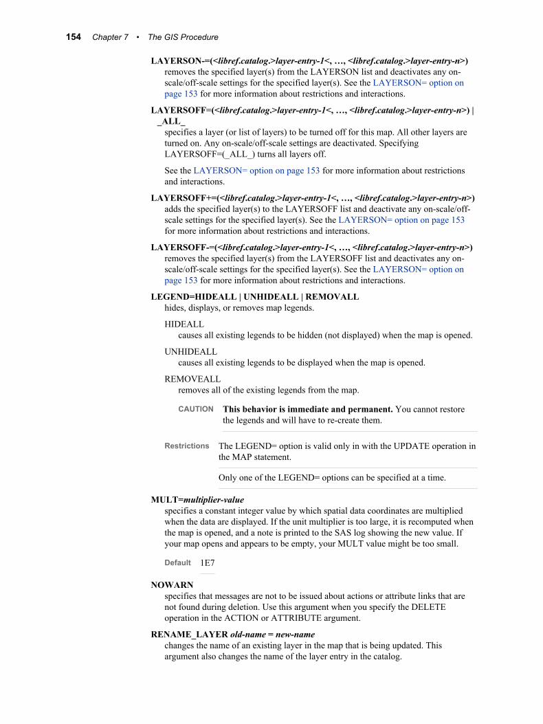
LAYERSON-=(<libref.catalog.>layer-entry-1<, …, <libref.catalog.>layer-entry-n>)removes the specified layer(s) from the LAYERSON list and deactivates any on-scale/off-scale settings for the specified layer(s). See the LAYERSON= option on page 153 for more information about restrictions and interactions.
LAYERSOFF=(<libref.catalog.>layer-entry-1<, …, <libref.catalog.>layer-entry-n>) | _ALL_
specifies a layer (or list of layers) to be turned off for this map. All other layers are turned on. Any on-scale/off-scale settings are deactivated. Specifying LAYERSOFF=(_ALL_) turns all layers off.
See the LAYERSON= option on page 153 for more information about restrictions and interactions.
LAYERSOFF+=(<libref.catalog.>layer-entry-1<, …, <libref.catalog.>layer-entry-n>)adds the specified layer(s) to the LAYERSOFF list and deactivate any on-scale/off-scale settings for the specified layer(s). See the LAYERSON= option on page 153 for more information about restrictions and interactions.
LAYERSOFF-=(<libref.catalog.>layer-entry-1<, …, <libref.catalog.>layer-entry-n>)removes the specified layer(s) from the LAYERSOFF list and deactivates any on-scale/off-scale settings for the specified layer(s). See the LAYERSON= option on page 153 for more information about restrictions and interactions.
LEGEND=HIDEALL | UNHIDEALL | REMOVALLhides, displays, or removes map legends.
HIDEALLcauses all existing legends to be hidden (not displayed) when the map is opened.
UNHIDEALLcauses all existing legends to be displayed when the map is opened.
REMOVEALLremoves all of the existing legends from the map.
CAUTION This behavior is immediate and permanent. You cannot restore the legends and will have to re-create them.
Restrictions The LEGEND= option is valid only in with the UPDATE operation in the MAP statement.
Only one of the LEGEND= options can be specified at a time.
MULT=multiplier-valuespecifies a constant integer value by which spatial data coordinates are multiplied when the data are displayed. If the unit multiplier is too large, it is recomputed when the map is opened, and a note is printed to the SAS log showing the new value. If your map opens and appears to be empty, your MULT value might be too small.
Default 1E7
NOWARNspecifies that messages are not to be issued about actions or attribute links that are not found during deletion. Use this argument when you specify the DELETE operation in the ACTION or ATTRIBUTE argument.
RENAME_LAYER old-name = new-namechanges the name of an existing layer in the map that is being updated. This argument also changes the name of the layer entry in the catalog.
154 Chapter 7 • The GIS Procedure

If other maps use the renamed layer, you must issue a MAP UPDATE statement for those maps as well.
SELECT=(<libref.catalog.>layer-entry-1<, …, <libref.catalog.>layer-entry-n>)lists the layers to be selectable when the map opens. All other layers will be unselectable.
SELECT+=(<libref.catalog.>layer-entry-1<, …, <libref.catalog.>layer-entry-n>)adds layers to the current list of selectable layers.
SELECT-=(<libref.catalog.>layer-entry-1<, …, <libref.catalog.>layer-entry-n>)removes layers from the current list of selectable layers.
UNSELECT=(<libref.catalog.>layer-entry-1<, …, <libref.catalog.>layer-entry-n>)lists the layers to be unselectable when the map opens. All other layers will be selectable.
UNSELECT+=(<libref.catalog.>layer-entry-1<, …, <libref.catalog.>layer-entry-n>)adds layers to the current list of unselectable layers.
UNSELECT-=(<libref.catalog.>layer-entry-1<, …, <libref.catalog.>layer-entry-n>)removes layers from the current list of unselectable layers.
DetailsA map entry is a SAS catalog entry of type GISMAP that defines the displayed features of a map. The definition specifies which layers the map contains and which coverage of the spatial database is used. The map entry also stores additional information. This includes legend definitions and action definitions for the map. It stores information about the projection system used to display the map. It stores the name of the data set that contains labels for map features. And it stores the names of any other associated SAS data sets.
Examples
Example 1: Define a New MapThe following code fragment creates an entry named STORES of type GISMAP in the current catalog. The map is based on the coverage defined in the GISCOVER entry named MALL in the current catalog. The map uses the GISLAYER entries STORE, FIRE, INFO, PHONE, and RESTROOM in the current catalog.
map create stores / coverage=mall layers=(store, fire, info, phone, restroom);run;
Example 2: Update an Existing Map DefinitionThe following code fragment updates the MAPS.USA.USA.GISMAP entry to use detail data when the map is displayed:
map update maps.usa.usa / details;run;
Example 3: Copy Attribute Data Set LinksThe following code fragment copies the SIMPLUSR attribute link from GISSIO.SIMPLUS.SIMPLE to WORK.SIMPLE.SIMPLE:
proc gis; map update work.simple.simple /
MAP Statement 155

attribute=(name=simplusr copy from=gissio.simplus.simple);run;
MAPLABEL StatementApplies, modifies, or deletes labels on a map.
SyntaxMAPLABEL operation <options>;
Summary of Optional Arguments
_ALL_applies an operation to all labels.
ATTACH_TO=MAP | WINDOWcontrols the label positioning and is a required argument.
COLOR=color-name | CXrrggbbspecifies the text color.
DATASET=<libref.>data-set-namespecifies the label data set to which new labels are appended.
FONT=font-name | DEFAULTspecifies the font used in the label.
FORCEreplaces the existing label data set reference in a map when both DATASET= and MAP= are specified.
FRONT | BACKcontrols how an image label is drawn relative to map features.
IMAGE='path-name' | <libref.>catalog.entry<.IMAGE> | filerefspecifies the location of an image to use as an image label on the map.
MAP=<libref.catalog.>map-entryindicates the map entry on which to display the labels.
OFFSCALE=(scale <units>)specifies a map scale at which the label is turned on off when the map view is zoomed.
OFFSET=(<x<units>> <, y<units>> <, units>)specifies the distance to move the entire label.
ONSCALE=(scale <units>)specifies a map scale at which the label is turned on when the map view is zoomed.
ORIGIN=(<x<unitx>> <, y<units>> <, units>)specifies the horizontal and vertical coordinates for the label.
OVERLAP | NOOVERLAPspecifies how labels are treated when they overlap.
POSITION=(<TOP | MIDDLE | BOTTOM> <LEFT | CENTER | RIGHT>)assigns a single label to a position on the map relative to the map's bounding box.
156 Chapter 7 • The GIS Procedure

ROW=integerspecifies the label in the data set to which the operation applies.
TEXT='string'specifies the text for a literal label.
TRANSPARENT | NOTRANSPARENTcontrols whether map features show though the label's bounding box.
OperationsCONTENTS
prints label information to the Output window. If you specify
• _ALL_, then every label not associated with a layer is printed.
• TEXT='string', then only labels matching that text are printed. The comparison is case sensitive.
• ROW=integer, then only the label at that row is printed.
If no labels are output, a NOTE is printed to the log.
CREATEcreates a new label or labels. Unlike CREATE operations for other PROC GIS statements, duplicate labels are allowed.
DELETEremoves the specified labels and, depending on which optional arguments are specified, possibly deletes the label data set. The only valid optional arguments for DELETE are DATASET=, MAP=, LAYER=, TEXT=, IMAGE=, ROW=, and _ALL_. Any others will be ignored.
If you specify
• DATASET=data-set-name as the only argument, then the label data set is deleted.
• MAP=map-entry as the only argument, then the label data set reference is removed from the map entry, and the data set is deleted. If you do not specify MAP=, and all of the rows in the label data set are deleted, you are cautioned. The caution indicates that any maps using the deleted data set will generate a WARNING when opened.
• ROW=, then only the label at that data set row is deleted. ROW= and _ALL_ are not allowed together. If you use ROW= and TEXT=, the TEXT= is ignored and the label at that row is deleted.
• TEXT='string', then every label literal having this exact string is removed from the label data set.
Note: Literal labels are those not associated with a specific layer.
• IMAGE=, then the specified image is deleted.
• _ALL_, then every label that is not associated with a layer is removed from the label data set.
Either DATASET= or MAP= is required or no deletions can occur.
Any DELETE operation that deletes all of the rows in the label data set also causes the data set to be deleted. If a data set is deleted, a NOTE is printed to the log. If MAP= is present and the label data set is deleted, the reference to the data set within the map entry is removed.
A note is printed in the log upon completion of a successful deletion.
MAPLABEL Statement 157

REPLACEreplaces an existing label specified by TEXT='string' of ROW=. If the label does not exist, a CREATE is performed.
UPDATEmodifies an existing label.
OptionsSeparate the list of options from the catalog entry name with a slash (/).
_ALL_affects the behavior of the following operations:
• In a CONTENTS operation, _ALL_ prints every label that is not associated with a layer to the Output window.
• In a DELETE operation, _ALL_ deletes every label that is not associated with a layer.
_ALL_ has no effect on CREATE, REPLACE, or UPDATE operations. If _ALL_ is detected, it is ignored.
_ALL_ cannot be used in the same statement with ROW= or TEXT= options.
ATTACH_TO=MAP | WINDOWcontrols the label positioning and is a required argument.
MAPThe label is attached to a location on the map. As you move the map in the window, the label moves with the map.
WINDOWThe label is attached to the map window. It remains fixed relative to the window as you move the map in the window.
COLOR=color-name | CXrrggbbspecifies the text color.
color-nameis a SAS color-name (for example, GREEN or RED).
CXrrggbbis an RGB color (for example, CX23A76B).
Default BLACK.
See For more information about color-naming schemes, see “Specifying Colors in SAS/GRAPH Programs” in SAS/GRAPH: Reference.
DATASET=<libref.>data-set-namespecifies the label data set to which new labels are appended. If the data set does not exist, it is created.
If you specify a one-level data set name, the WORK library is assumed. If you specify both DATASET= and MAP=, and the map already references a label data set, the data set names are compared. If they are not the same and FORCE was not specified, a warning is printed, and the run group is terminated.
FONT=font-name | DEFAULTspecifies the font used in the label.
font-namespecifies a font for the label text.
158 Chapter 7 • The GIS Procedure

Default If the specified font is not found when the map is opened, the default system font is substituted and a note is printed to the log.
Example font='Times New Roman-12pt-Roman-Bold'font='Display Manager font'font='Sasfont (10x15) 10pt-9.7pt-Roman-Normal'
DEFAULTassigns the default font to the label.
FORCEreplaces the existing label data set reference in a map when both DATASET= and MAP= are specified. If the map already references a label data set, its data set name is compared to the name specified with DATASET=. If they are not the same, the FORCE option causes the map's label data set reference to be overwritten and a note printed to the log. The map's original label data set is not deleted.
FRONT | BACKcontrols how an image label is drawn relative to map features.
FRONTcauses an image label to be drawn over the map features.
BACKcauses an image label to be drawn beneath the map features.
Default FRONT
Note These options do not apply to text labels.
IMAGE='path-name' | <libref.>catalog.entry<.IMAGE> | filerefspecifies the location of an image to use as an image label on the map.
'path-name'specifies a host directory path to an image file.
Example image='C:\My SAS Files\photo.gif'
<libref.>catalog.entry<.IMAGE>specifies an IMAGE type catalog entry for the image label.
If you omit the library name from the statement, the WORK library is the default.
filerefspecifies an active SAS fileref that points to an external file for an image label. The host directory path for this fileref is written to the label data set, not to the fileref.
MAP=<libref.catalog.>map-entryindicates the map entry on which to display the labels. If you specify a one-level name, the map entry is assumed to be in one of two catalogs. It will be the catalog that is specified in the PROC GIS statement or in the most recently issued CATALOG statement.
If the specified map entry already references a label data set, new labels are appended to that data set.
If the map entry does not reference a label data set, you must provide a label data set name with the DATASET= option. The labels are written to that data set, and the data set is then assigned to the specified map.
MAPLABEL Statement 159

For the MAPLABEL statement, either MAP= or DATASET= is required. If both are present and the map already has a label data set, its name must match the name specified in the DATASET= option. One exception is if the FORCE option is also used. In that case, the label data set specified by DATASET= is assigned to the map entry. The map's original label data set is unassigned but not deleted.
OFFSET=(<x<units>> <, y<units>> <, units>)specifies the distance to move the entire label.
xis the number of units to move the label right (positive numbers) or left (negative numbers).
yis the number of units to move the label up (positive numbers) or down (negative numbers).
unitsis one of the following values:
PERCENT | PCTspecifies that the X and Y coordinate values are a percentage of the distance from the lower left corner of the map window to the label origin. When the window is resized, the label remains in the same relative location. For example, if both the X and Y coordinates are set to 50, then the label origin remains in the center of the window. Negative values and values greater than 100% are not allowed.
PIXELspecifies that the X and Y coordinate values are screen coordinates using pixels. The lower left corner of the window is 0, 0. Negative values are not allowed. If a specified pixel value runs the label outside of the window, the label is shifted. The shift can be horizontal, vertical, or both so that the label is placed just within the window when the map is opened.
REALX and Y values are real-world coordinates based on the underlying spatial data. Negative values can be used to signify the western or southern hemispheres if the spatial data contains them.
To set only the X offset, specify one value, with or without a following comma, as in the following example:
offset = ( 10 real, )
To set both the X and Y offset, specify two values, with or without a comma separating them, as in the following example:
offset = ( 20 pct, 40 pct )
To set only the Y offset, specify one value preceded by a comma, as in the following example:
offset = ( ,-30 pct )
OFFSET= is usually used in conjunction with POSITION= to adjust the position of a label. Moves are relative to the location specified by POSITION=, with OFFSET=(0,0) representing the initial position. You can also apply OFFSET= to the default label position.
The following restrictions apply to the OFFSET= argument:
160 Chapter 7 • The GIS Procedure

• When both ORIGIN and OFFSET are used, the same units must be specified for both. If no units are specified in the OFFSET= arguments, the unit entered in the ORIGIN= option is used.
• OFFSET= is unnecessary with ORIGIN= because ORIGIN= explicitly positions the label and requires no further adjustment. However, if you specify both options, the values of OFFSET= are added to the values of ORIGIN=, and the label is positioned accordingly.
• If the resulting location is outside of the GIS Map window, a warning is printed to the log when the map is opened. The label is moved to be within the window.
ONSCALE=(scale <units>)specifies a map scale at which the label is turned on when the map view is zoomed.
scalespecifies the map scale value at which the label is turned on.
unitsspecifies the units for the scale value.
real-units/map-unitsenables you to specify various combinations of units. Valid values are KM, M, CM, MI, FT, and IN. Real-units is typically KM, M, MI, or FT, and map-units is usually either CM or IN. Long forms of the unit names (for example, KILOMETERS or INCH (singular or plural), are also acceptable).
METRICsets the scale units to KM/CM (kilometers per centimeter).
ENGLISHsets the scale units to MI/IN (miles per inch).
Default METRIC
OFFSCALE=(scale <units>)specifies a map scale at which the label is turned on off when the map view is zoomed.
scalespecifies the map scale value at which the label is turned off.
unitsspecifies the units for OFFSCALE.
real-units/map-unitsenables you to specify various combinations of units. Valid values are KM, M, CM, MI, FT, and IN. Real-units is typically KM, M, MI, or FT, and map-units is usually either CM or IN. Long forms of the unit names (for example, KILOMETERS or INCH (singular or plural), are also acceptable).
METRICsets the scale units to KM/CM (kilometers per centimeter).
ENGLISHsets the scale units to MI/IN (miles per inch).
Default METRIC
ORIGIN=(<x<unitx>> <, y<units>> <, units>)specifies the horizontal and vertical coordinates for the label. ORIGIN= explicitly positions the label anywhere on the map. Unlike the POSITION= location, the label
MAPLABEL Statement 161

is not centered about this point. The lower left corner of the label is placed at the specified ORIGIN location.
xspecifies the X coordinate (horizontal axis)
yspecifies the Y coordinate (vertical axis)
unitscan be one of the following values:
PERCENT | PCTspecifies that the X and Y coordinate values are a percentage of the distance from the lower left corner of the map window to the label origin. When the window is resized, the label remains in the same relative location. For example, if both the X and Y coordinates are set to 50, then the label origin remains in the center of the window. Negative values and values greater than 100% are not allowed.
PIXELspecifies that the X and Y coordinate values are screen coordinates using pixels. The lower left corner of the window is 0, 0. Negative values are not allowed. If a specified pixel value runs the label outside of the window, the label is shifted. The label shifts horizontally, vertically, or both to be just within the window when the map is opened.
REALX and Y values are real-world coordinates based on the underlying spatial data. Negative values can be used to signify the western or southern hemispheres if the spatial data contains them.
To set only the X coordinate, specify one value with or without a following comma, as in the following examples:
origin=(10 pixels,)origin=(10 pixels)
To set both the X and Y coordinates, specify two values with or without a comma separating them. The units can be specified for both X and Y or once at the end, as in the following examples:
origin=(10 pct, 40 pct)origin=(10 pct 40 pct)origin=(10 40 pct)origin=(10, 40, pct)
To set only the Y coordinate, specify one value preceded by a comma, as in the following example:
origin=(, 20 pct)
ORIGIN= overrides the POSITION= option if both options are present. Although using the OFFSET= option with the ORIGIN= option is unnecessary, if you also specify OFFSET=, it is applied after the ORIGIN= request has been processed.
If the specified origin or origin plus offset is outside of the overall map bounding box, a warning is printed to the log. No warning is issued if the label runs out of the box, however.
OVERLAP | NOOVERLAPspecifies how labels are treated when they overlap.
162 Chapter 7 • The GIS Procedure

OVERLAPAll labels that you create with the option will be displayed even if they conflict with other labels.
NOOVERLAPSome of the conflicting labels will be suppressed until you zoom in more closely.
Default NOOVERLAP
POSITION=(<TOP | MIDDLE | BOTTOM> <LEFT | CENTER | RIGHT>)assigns a single label to a position on the map relative to the map's bounding box. If the label is attached to the map, the label position is determined using the spatial data bounding box. The bounding box is the upper, lower, right and left edges of the coverage extents. If the label is attached to the window, the window edges are used.
The following arguments determine the vertical position of the label:
TOPplaces the label along the upper edge of the map or window.
MIDDLEplaces the label halfway between the top and bottom edges of the map or window.
BOTTOMaligns the label with the bottom edge of the map or window.
The following arguments determine the horizontal position of the label:
LEFTstarts the label at the left edge of the map or window.
CENTERplaces the label halfway between the left and right edges of the map or window.
RIGHTaligns the end of the label with the right edge of the map or window. The label is centered horizontally and vertically at the computed position point. You can adjust the initial label position with the OFFSET= option.
ROW=integerspecifies a particular label in the data set to UPDATE, REPLACE, DELETE or print CONTENTS. Not valid for CREATE operations.
TEXT='string'specifies the text for a literal label. For REPLACE, UPDATE, DELETE or CONTENTS operations, string specifies a search string used to locate a specific target label. When TEXT='string' is used to search for a label, string is case sensitive, and an exact match to the value of the search string must be found. For example, TEXT='Paris' will ignore a label having PARIS as its text. It will also ignore a label having 'Paris Metro' as its text.
If ROW= and TEXT= are both present in a REPLACE or UPDATE statement the 'string' entered with TEXT= is not a search string. It becomes the new text for the label at the specified ROW number.
TRANSPARENT | NOTRANSPARENTcontrols whether map features show though the label's bounding box.
TRANSPARENTenables the map features to show though the label's bounding box.
NOTRANSPARENTblocks the display of map features within the label's rectangular bounding box.
MAPLABEL Statement 163

These options apply to text labels and image labels stored as catalog entries. They have no effect on image labels stored in an external file.
Default TRANSPARENT
COPY StatementCopies a SAS/GIS catalog entry or data set.
Note: You can copy a single GIS entry or include the dependent entries and data sets that are referenced by the source.
SyntaxCOPY <libref.catalog.>entry-name<.type> </ options> ;
Summary of Optional Arguments
ALIAS=(old-libref-1=new-libref-1<, …, old-libref-n=new-libref-n>)specifies libref translations.
BLANKspecifies that internal pathnames should be cleared in the copied entries.
DESTCAT=libref.catalogspecifies the destination for the copied catalog entries.
DESTLIB=librefspecifies the destination library for the copied data sets.
ENTRYTYPE=typespecifies the type of GIS catalog entry to copy.
REPLACEspecifies that both existing catalog entries and data sets that have the same name as copied entries and data sets should be overwritten.
SELECT=_ALL_ | ENTRY | DATASETS | LABEL | OTHER | NOSOURCE | SPATIAL
specifies which data sets or catalog entries that are referenced by the source entry should be copied.
Required Argument<libref.catalog.>entry<.type>
specifies the catalog entry to copy. If you specify a one-level name, the current catalog is used.
Note When you specify a four-level entry name, type must be the actual SAS/GIS catalog entry extension (for example, GISMAP, not MAP).
164 Chapter 7 • The GIS Procedure
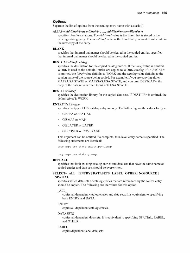
OptionsSeparate the list of options from the catalog entry name with a slash (/).
ALIAS=(old-libref-1=new-libref-1<, …, old-libref-n=new-libref-n>)specifies libref translations. The old-libref value is the libref that is stored in the existing catalog entry. The new-libref value is the libref that you want to substitute in the new copy of the entry.
BLANKspecifies that internal pathnames should be cleared in the copied entries. specifies that internal pathnames should be cleared in the copied entries.
DESTCAT=libref.catalogspecifies the destination for the copied catalog entries. If the libref value is omitted, WORK is used as the default. Entries are copied to WORK.catalog. If DESTCAT= is omitted, the libref value defaults to WORK and the catalog value defaults to the catalog name of the source being copied. For example, if you are copying either MAPS.USA.STATE or MAPSSAS.USA.STATE, and you omit DESTCAT=, the copy of the data set is written to WORK.USA.STATE.
DESTLIB=librefspecifies the destination library for the copied data sets. If DESTLIB= is omitted, the default libref is WORK.
ENTRYTYPE=typespecifies the type of GIS catalog entry to copy. The following are the values for type:
• GISSPA or SPATIAL
• GISMAP or MAP
• GISLAYER or LAYER
• GISCOVER or COVERAGE
This argument can be omitted if a complete, four-level entry name is specified. The following statements are identical:
copy maps.usa.state entrytype=gismap
copy maps.usa.state.gismap
REPLACEspecifies that both existing catalog entries and data sets that have the same name as copied entries and data sets should be overwritten.
SELECT=_ALL_ | ENTRY | DATASETS | LABEL | OTHER | NOSOURCE | SPATIAL
specifies which data sets or catalog entries that are referenced by the source entry should be copied. The following are the values for this option:
_ALL_copies all dependent catalog entries and data sets. It is equivalent to specifying both ENTRY and DATA.
ENTRYcopies all dependent catalog entries.
DATASETScopies all dependent data sets. It is equivalent to specifying SPATIAL, LABEL, and OTHER.
LABELcopies dependent label data sets.
COPY Statement 165

NOSOURCEcopies entry dependents as specified, but does not copy the specified source entry.
OTHERcopies other dependent data sets (besides spatial and label data sets), such as linked attribute data sets.
SPATIALcopies dependent spatial data sets.
DetailsYou can use PROC COPY or another utility to copy a SAS/GIS catalog entry or data set. However, you might receive warnings in your SAS log that the paths are not the same. If you receive a message that the paths are not the same, you can use the SYNC statement to reset the paths. See “SYNC Statement” on page 168 for more information.
MOVE StatementMoves a SAS/GIS catalog entry or data set.
Notes: You can move a single GIS entry or include the dependent entries and data sets that are referenced by the source.The MOVE statement deletes the original entry or data set and creates a new copy in the target directory. If you do not have Write permission to the source location, MOVE leaves the original entry or data set in its directory and creates a copy in the target directory.
SyntaxMOVE <libref.catalog.>entry-name<.type> </ options>;
Summary of Optional Arguments
ALIAS=(old-libref-1=new-libref-1<, …, old-libref-n=new-libref-n>)specifies libref translations.
BLANKspecifies that internal pathnames should be cleared in the moved entries.
CHECKPARENTspecifies that data sets and catalog entries are checked before they are moved to see what other GIS entries references them.
DESTCAT=libref.catalogspecifies the destination for the moved catalog entries.
DESTLIB=librefspecifies the destination library for the moved data sets.
ENTRYTYPE=typespecifies the type of GIS catalog entry to move.
REPLACEspecifies that both existing catalog entries and data sets that have the same name as moved entries and data sets should be overwritten.
SELECT=_ALL_ | ENTRY | DATASETS | SPATIAL | LABEL | OTHER | NOSOURCE
166 Chapter 7 • The GIS Procedure

specifies which data sets or catalog entries that are referenced by the source entry should be moved.
Required Argument<libref.catalog.>entry<.type>
specifies the catalog entry to move. If you specify a one-level name, the current catalog is used.
Note When you specify a four-level entry name, type must be the actual SAS/GIS catalog entry extension (for example, GISMAP, not MAP).
OptionsSeparate the list of options from the catalog entry name with a slash (/).
ALIAS=(old-libref-1=new-libref-1<, …, old-libref-n=new-libref-n>)specifies libref translations. The old-libref value is the libref that is stored in the existing catalog entry. The new-libref value is the libref that you want to substitute in the moved entry.
BLANKspecifies that internal pathnames should be cleared in the moved entries.
CHECKPARENTspecifies that data sets and catalog entries are checked before they are moved to see what other GIS entries references them. If any references are found, the catalogs and data sets are copied instead of being moved.
If CHECKPARENT is not specified, data sets and catalog entries are moved without checking for references, which might cause problems with other GIS entries.
Default CHECKPARENT
CAUTION Do not use host commands to move or rename SAS data sets that are referenced in GISSPA entries. Moving or renaming a data set that is referred to in a spatial entry breaks the association between the spatial entry and the data set. To prevent breaking the association, use the PROC GIS MOVE statement with the CHECKPARENT option instead of a host command.
DESTCAT=libref.catalogspecifies the destination for the moved catalog entries. If the libref value is omitted, WORK is used as the default. Entries are moved to the WORK.catalog. If DESTCAT= is omitted, then the libref value defaults to WORK and the catalog value defaults to the catalog name of the source being moved. For example, if you are moving either MAPS.USA.STATE or MAPSSASUSA.STATE, and you omit DESTCAT=, the data set that you are moving is written to WORK.USA.STATE.
DESTLIB=librefspecifies the destination library for the moved data sets. If DESTLIB= is omitted, the default libref is WORK.
ENTRYTYPE=typespecifies the type of GIS catalog entry to move. The following are the values for type:
• GISSPA or SPATIAL
• GISMAP or MAP
MOVE Statement 167

• GISLAYER or LAYER
• GISCOVER or COVERAGE
This argument can be omitted if a complete, four-level entry name is specified. The following statements are identical:
move maps.usa.state entrytype=map
move maps.usa.state.gismap
REPLACEspecifies that both existing catalog entries and data sets that have the same name as moved entries and data sets should be overwritten.
SELECT=_ALL_ | ENTRY | DATASETS | SPATIAL | LABEL | OTHER | NOSOURCE
specifies which data sets or catalog entries that are referenced by the source entry should be moved. The following are the values for this argument:
_ALL_moves all dependent catalog entries and data sets. Equivalent to specifying both ENTRY and DATA.
DATAmoves all dependent data sets. It is equivalent to specifying SPATIAL, LABEL, and OTHER.
ENTRYmoves all dependent catalog entries.
LABELmoves dependent label data sets.
NOSOURCEmoves entry dependents as specified, but does not move the specified source entry.
OTHERmoves other dependent data sets (besides spatial and label data sets), such as linked attribute data sets.
SPATIALmoves dependent spatial data sets.
DetailsYou can use PROC COPY or another utility to move a SAS/GIS catalog entry or data set. However, you might receive warnings in your SAS log that the paths are not the same. If you receive a message that the paths are not the same, you can use the SYNC statement to reset the paths. See “SYNC Statement” on page 168 for more information.
SYNC StatementUpdates a SAS/GIS catalog entry libref and the internal pathname.
Restriction: In order to use the SYNC statement on a catalog entry, you must have Write permission to the source location.
Note: You can synchronize a single GIS entry or include the dependent entries on a catalog entry.
168 Chapter 7 • The GIS Procedure

SyntaxSYNC <libref.catalog.>entry<.type> </ options>;
Summary of Optional Arguments
ALIAS=(old-libref-1=new-libref-1<, …, old-libref-n=new-libref-n>)specifies libref translations.
BLANKspecifies that internal pathnames should be cleared in the updated entries.
ENTRYTYPE=typespecifies the type of GIS catalog entry to synchronize.
SELECT=_ALL_ | ENTRYspecifies which catalog entries that are referenced by the source entry should be updated.
Required Argument<libref.catalog.>entry<.type>
specifies the catalog entry to synchronize. If you specify a one-level name, the current catalog is used.
Note When you specify a four-level entry name, type must be the actual SAS/GIS catalog entry extension (for example, GISMAP, not MAP).
OptionsSeparate the list of options from the catalog entry name with a slash (/).
ALIAS=(old-libref-1=new-libref-1<, …, old-libref-n=new-libref-n>)specifies libref translations. The old-libref value is the libref that is stored in the existing catalog entry. The new-libref value is the libref that you want to substitute in the synchronized version of the entry.
BLANKspecifies that internal pathnames should be cleared in the updated entries.
ENTRYTYPE=typespecifies the type of GIS catalog entry to synchronize. The following are the values for type:
• GISSPA or SPATIAL
• GISMAP or MAP
• GISLAYER or LAYER
• GISCOVER or COVERAGE.
This argument can be omitted if a complete, four-level entry name is specified. The following statements are identical:
sync sasuser.mall.stores entrytype=gismap
sync sasuser.mall.stores.gismap
SELECT=_ALL_ | ENTRYspecifies which catalog entries that are referenced by the source entry should be updated. The following are the values for this argument:
SYNC Statement 169

_ALL_updates all dependent catalog entries. This is equivalent to specifying ENTRY.
ENTRYupdates all dependent catalog entries.
170 Chapter 7 • The GIS Procedure

Appendix 1
Sample Map Data Sets
Map and Data Sets Supplied with SAS/GIS Software . . . . . . . . . . . . . . . . . . . . . . 171
Maps in the USA Catalog . . . . . . . . . . . . . . . . . . . . . . . . . . . . . . . . . . . . . . . . . . . . . . 171
Maps in the NC Catalog . . . . . . . . . . . . . . . . . . . . . . . . . . . . . . . . . . . . . . . . . . . . . . . 173
Maps in the WAKE Catalog . . . . . . . . . . . . . . . . . . . . . . . . . . . . . . . . . . . . . . . . . . . 174
Copying and Modifying SAS/GIS Maps in the MAPS or MAPSSAS Library . . . 175
Maps Produced by the SAS/GIS Tutorial . . . . . . . . . . . . . . . . . . . . . . . . . . . . . . . . 176
Map and Data Sets Supplied with SAS/GIS Software
Several SAS/GIS sample maps and their associated data sets are supplied with SAS/GIS software. These maps reside in both the MAPS and MAPSSAS libraries, along with map data sets shipped with SAS/GRAPH software.These maps can be used for exploring the software or for demonstration purposes.
To open the sample maps, invoke SAS/GIS and select File ð Open Map or right-click the GIS Map window and select Open Map. Select the MAPS or MAPSSAS library, followed by the catalog and the map name.
Three sets of sample maps are included with SAS/GIS software, and two maps are created by the SAS/GIS Tutorial. The following list provides the name of the map, and the spatial data sets, catalogs, and data sets associated with each map. The format of the map name is either MAPS.catalog.map-name or MAPSSAS.catalog.map-name.
Additional maps can be created using the SAS/GIS import process.
Maps in the USA CatalogThese maps are all defined in the same spatial database. That is, they all use the same spatial data even though the maps represent different geographic areas.
MAPS.USA.STATE or MAPSSAS.USA.STATEEither map includes USA and STATE boundaries for the continental United States, along with a CAP_CITY layer that represents the locations of state capitals. The theme defined for the STATE layer depicts average household income by state. A
171

Browse action named BRSTATE displays information about the selected state. A Drill action defined for this map allows users to drill down to an individual county map of the selected state. Selecting the state of North Carolina and running the DRILL action opens a sample map of North Carolina by COUNTY and ZIP code (MAPS.NC.NC).
MAPS.USA.COUNTY or MAPSSAS.USA.COUNTYEither map includes USA, STATE, and COUNTY boundaries for the continental United States. The theme defined for the COUNTY layer depicts population change by county. There are three actions defined for this map. A Browse action named BRCOUNTY displays information about the selected county. The TREND Program action creates a bar chart that displays population and housing trends. A Program action named RATIO creates a plot that displays population and housing ratios for the selected county.
MAPS.USA.TRAINING or MAPSSAS.USA.TRAININGEither map includes USA and STATE boundaries for the continental United States, along with a CENTER point layer that represents the locations of SAS Training Centers. This map contains an IMAGE action that displays a picture of the selected training center. There is also a Browse action named BRCENTER that displays information about the selected training center.
MAPS.USA.state or MAPSSAS.USA.state(where state is the two-character postal code for the state)
There is an individual map for every state in the continental United States, plus the District of Columbia. Each map is named using the two-character postal code for the particular state. These maps include USA, STATE, and COUNTY boundaries. The theme defined for the COUNTY layer is the same as in the MAPS.USA.COUNTY or MAPSSAS.USA.COUNTY map, and depicts population change by county. There are three actions defined for the maps. A Browse action named COUNTY displays information about a selected county. The TREND Program action creates a bar chart that displays population and housing trends. A Program action named RATIO creates a plot that displays population and housing ratios for a selected county.
Associated catalog and data sets:
Table A1.1 Catalog and Data Sets Associated with MAPS.USA or MAPSSAS.USA
USA Catalog
USAC Chains data set
USAN Nodes data set
USAD Details data set
USACTI Polygonal index data set for the COUNTY layer
USASTI Polygonal index data set for the STATE layer
USACTLAB Label data set for the COUNTY map
USALAB Label data set for the TRAINING map
USASTLAB Label data set for the STATE map
172 Appendix 1 • Sample Map Data Sets

USAAC Attribute data set for the COUNTY map
USAAS Attribute data set for the STATE map
USAAT Attribute data set for the TRAINING map
Maps in the NC CatalogMAPS.NC.NC or MAPSSAS.NC.NC
This map consists of COUNTY and ZIP code boundaries in North Carolina, along with a CITY layer representing the locations of major cities. A Drill action defined for this map enables users to drill down to a map of Wake County (MAPS.WAKE.TRACT) by selecting Wake County and running the DRILL action. This map contains three additional actions that can be run for the selected ZIP code:
• A Browse action that displays population and household data.
• A Program action named SUMMARY that executes a MEANS procedure and produces a summary for the ZIP code.
• A Program action named TREND that produces a line graph depicting population and housing trends.
Associated catalog and data sets:
Table A1.2 Catalog and Data Sets Associated with MAPS.NC or MAPSSAS.NC
NC Catalog
NCC Chains data set
NCN Nodes data set
NCD Details data set
NCCTI Polygonal index data set for the COUNTY layer
NCZIPI Polygonal index data set for the ZIP layer
NCCTLAB Label data set for the CITY layer
NCLAB Label data set for the CITY layer
NCWKLAB Label data set for the COUNTY layer (Wake County)
NCAZ Attribute data set
Maps in the NC Catalog 173

Maps in the WAKE CatalogThese maps are all defined in the same spatial database. That is, they all use the same spatial data even though the maps are not identical.
MAPS.WAKE.BG or MAPSSAS.WAKE.BGThis map includes COUNTY, TRACTS, and BG (block group) boundaries, as well as a STREET layer, for Wake County, North Carolina. The theme defined for the BG layer depicts the number of households by block group. This map includes a Browse action named CENSUS that displays information about the selected block group.
MAPS.WAKE.GROCERY or MAPSSAS.WAKE.GROCERYThis map includes COUNTY and TRACT boundaries for Wake County, North Carolina, as well as a STREET layer and a GROCERY layer, which represents the locations of grocery stores. The theme defined for the TRACT layer depicts the average household income by tract. This map includes three actions: a Program action named GRAPH that produces a bar chart of store size versus sales for the selected store; a Browse action that displays information about the selected store; and a Spatial action that displays spatial information about the selected store.
MAPS.WAKE.TRACT or MAPSSAS.WAKE.TRACTThis map includes COUNTY and TRACT boundaries for Wake County, North Carolina, as well as a STREET layer. The theme defined for the TRACT layer depicts the neighborhood type by tract. This map includes a Browse action that displays demographic information about the selected tracts.
Associated catalog and data sets:
Table A1.3 Catalog and Data Sets Associated with MAPS.WAKE or MAPSSAS.WAKE
WAKE Catalog
WAKEC Chains data set
WAKEN Nodes data set
WAKED Details data set
WAKEBGI Polygonal index data set for the BG layer
WAKETRTI Polygonal index data set for the TRACTS layer
WAKELAB Label data set
WAKEABG Attribute data set for the BG map
WAKEAG Attribute data set for the GROCERY map
WAKEAT Attribute data set for the TRACT map
174 Appendix 1 • Sample Map Data Sets

Copying and Modifying SAS/GIS Maps in the MAPS or MAPSSAS Library
Most SAS software users do not have Write permission to the MAPS or MAPSSAS libraries. As a result, you will not be able to save any changes that you make to the SAS/GIS sample maps. You will see an error similar to the following in your SAS Log if you try to save any changes made to these maps:
ERROR: Write access to member MAPS.NC.CATALOG is denied.
In order to save modifications to these maps, you must first copy the map and its associated data sets to a SAS library to which you have Write access. Use the Copy utility included with SAS/GIS to copy the maps.
For example, to copy the MAPS.NC.NC map and its associated data sets from the MAPS library to the SASUSER library, invoke SAS/GIS, select Edit ð Copy
Follow these steps:
1. Enter or browse and select MAPS.NC.NC for the Entry field.
2. Select Map as the entry Type.
3. In the Catalog Entry Destination field, enter the library and catalog to which you will be copying the map. You must specify a currently allocated SAS library. If the specified catalog does not already exist in the library, it will be created during the copy process. In this example, enter SASUSER.NC.
4. In the Options box, select all options:
• Copy Source Entry
• Copy Dependent Entries
• Copy Dependent Data Sets
• Spatial Label Other
• Replace Like-Named Entries/Data Sets
• Blank out Path Name References
5. In the Data Set Destination field, enter the library to which the data sets associated with the map will be copied. In this case, enter SASUSER.
6. Click the Apply button to begin copying the map. When the copy is complete, you will see a note in the message line similar to the following:
Number of entries, data sets copied: 9, 8
You will also see a list in the SAS Log window of all of the catalogs and data sets that were copied.
Now open the SASUSER.NC.NC map in the GIS Map window. You will now be able to make any desired modifications to the map, and save those modifications to the copied map.
Copying and Modifying SAS/GIS Maps in the MAPS or MAPSSAS Library 175

Maps Produced by the SAS/GIS TutorialTwo sample maps are produced by the SAS/GIS Tutorial. The maps are created automatically when the tutorial is invoked by selecting Help ð Getting Started with SAS/GIS Software ð Begin Tutorial from the GIS Map window. You can also create the maps without invoking the Tutorial by selecting Help ð Getting Started with SAS/GIS Software ð Create Data.
These maps are created in the SASUSER library, so changes made to these maps can be saved. The following list provides the name of the map, and the spatial data sets, catalogs, and data sets associated with each map. These two maps are defined in the same spatial database. That is, they use the same spatial data even though the maps are not identical.
SASUSER.MALL.AREAThis map includes TRACT boundaries for several tracts in Wake County, North Carolina. The map also includes point layers MALL, PARK, and SCHOOL. The map does not have a theme defined for the TRACT layer. A STREET layer is also included in this map. A Drill action defined for the MALL layer allows users to drill down to a detailed floor plan of a mall (SASUSER.MALL.STORES).
Associated catalog and data sets:
Table A1.4 Catalog and Data Sets Associated with SASUSER.MALL.AREA
MALL Catalog
MALLC Chains data set
MALLN Nodes data set
MALLD Details data set
MALLTI Polygonal index data set for the TRACT layer
MALLPOP Attribute data set
SASUSER.MALL.STORESThis map consists of STORE and ATRIUM boundaries for a fictitious shopping mall. The map includes FIRE and SPRINK line layers, which depict fire exits and sprinkler systems, as well as the following point layers: INFO, PHONE, RESTROOM, STROLLER, SECURITY, and ALARM.
There are two actions defined for this map. The STOREPIC image action displays a picture of a store when one of the areas of the STORE layer is selected. The CHART Program action creates a bar chart of the square footage of the selected store(s).
Associated catalog and data sets:
Table A1.5 Catalog and Data Sets Associated with SASUSER.MALL.STORES
MALL Catalog
176 Appendix 1 • Sample Map Data Sets

MALLC Chains data set
MALLN Nodes data set
MALLD Details data set
MALLSI Polygonal index data set for the STORE layer
MALLAI Polygonal index data set for the ATRIUM layer
MALLSTOR Attribute data set
Maps Produced by the SAS/GIS Tutorial 177

178 Appendix 1 • Sample Map Data Sets

Appendix 2
Spatial Database Details
The SAS/GIS Data Model . . . . . . . . . . . . . . . . . . . . . . . . . . . . . . . . . . . . . . . . . . . . . 179SAS/GIS Data Types . . . . . . . . . . . . . . . . . . . . . . . . . . . . . . . . . . . . . . . . . . . . . . . 179Spatial Data Features . . . . . . . . . . . . . . . . . . . . . . . . . . . . . . . . . . . . . . . . . . . . . . . 179SAS/GIS Topology . . . . . . . . . . . . . . . . . . . . . . . . . . . . . . . . . . . . . . . . . . . . . . . . . 180Rules for Topological Correctness . . . . . . . . . . . . . . . . . . . . . . . . . . . . . . . . . . . . . 180Attribute Data Features . . . . . . . . . . . . . . . . . . . . . . . . . . . . . . . . . . . . . . . . . . . . . . 182
SAS/GIS Spatial Database Structure . . . . . . . . . . . . . . . . . . . . . . . . . . . . . . . . . . . . 182Overview . . . . . . . . . . . . . . . . . . . . . . . . . . . . . . . . . . . . . . . . . . . . . . . . . . . . . . . . . 182Spatial Data Sets . . . . . . . . . . . . . . . . . . . . . . . . . . . . . . . . . . . . . . . . . . . . . . . . . . . 182Catalog Entries . . . . . . . . . . . . . . . . . . . . . . . . . . . . . . . . . . . . . . . . . . . . . . . . . . . . 186
Composites . . . . . . . . . . . . . . . . . . . . . . . . . . . . . . . . . . . . . . . . . . . . . . . . . . . . . . . . . . 190
The SAS/GIS Data Model
SAS/GIS Data TypesSAS/GIS software uses two basic types of data:
spatial datadescribes the location, shape, and interrelationships of map features.
attribute dataprovides information that relates to the map features.
Spatial Data FeaturesSAS/GIS software uses spatial data to represent the following three types of map features:
point featuresconsist of individual locations that are shown as symbols, representing real-world locations of special points of interest.
line featuresconsist of sequences of two or more coordinates that form zero-width shapes, either closed or unclosed. Line features represent entities that either have no width, such as political boundaries, or those that can be represented as having no width, such as streets or water pipes.
179

area featuresconsist of sequences of three or more coordinates that form polygons (with single or multiple boundaries and with or without holes.) Area features represent two-dimensional entities such as geographic areas (countries, states, and so on) or floor plans for buildings.
SAS/GIS TopologyTo represent point, line, and area features in a map, SAS/GIS software defines the following topological features in the spatial data:
chainsare sequences of two or more points in the coordinate space. The end points (that is, the first and last points of the chain) are nodes. Each chain has a direction, from the first point toward the last point. The first point in the chain is the from-node and the last point is the to-node. Relative to its direction, each chain has a left side and a right side.
Points between the from-node and the to-node are detail points, which serve to trace the curvature of the feature that is represented by the chain. Detail points are not nodes.
nodesare points in the spatial data coordinate space that have connections to one or more chains.
areasare two-dimensional finite regions of the coordinate space. One or more chains, called boundary chains, separate two different areas. Chains that lie completely inside an area are called internal chains and are bounded on the left and right sides by the same area.
The spatial data coordinate space can be represented in any numeric units, even those that include arbitrary values. Coordinates that are stored as longitude and latitude values have a maximum usable precision of about one centimeter.
Representations of map features are implemented with one or more chains, as follows:
point featuresare implemented with one chain, one node (that is, the from-node and to-node for a point feature are the same node), and no detail points.
line and area featuresare implemented with one or more chains and one or more nodes.
Rules for Topological Correctness
OverviewSAS/GIS spatial data must obey the following rules in order for the topology to be correct. These rules are similar to the rules for TIGER files from the U.S. Census Bureau. For more information about these rules, see Gerard Boudriault's 1987 article, “Topology in the TIGER File” in AUTO-CARTA 8, Proceedings, pages 258-263, published by the American Society for Photogrammetry and Remote Sensing and the American Congress on Surveying and Mapping.
180 Appendix 2 • Spatial Database Details

Topological CompletenessAll chains must have the following characteristics:
• They must be bounded by two nodes, the from-node and the to-node.
Note: There is a special circumstance regarding chains for point features, for single-chain closed-loop line features, or for area boundaries. The from-node and the to-node are the same node, but both nodes are still included in the chain definition.
• They must be bounded by two areas, one on the left and one on the right.
These relationships must be complete, so the following two rules apply:
• The sides of all the chains incident to any given node must form a cycle. A cycle consists of one or more chains that start or end at the same node.
• The end points of chains that bound an area must form one or more disjoint cycles.
For each unique area ID or unique set of area IDs, all the boundary chains with the ID value form one or more closed loops or cycles. However, the boundary chains must be either on the right or the left, but not on both sides.
Topological-geometric ConsistencyThe collection of chains, nodes, and areas must have coordinates that make the collection a disjoint partitioning of the coordinate space. The following four conditions must be true to avoid problems with displaying the spatial data:
• No two points in the combined set of nodes and detail points can share the same coordinate.
• No two line segment interiors can share a common coordinate.
• No two areas can share a common coordinate.
Note: Graphically overlaid data can have overlapping polygons, chains, and nodes and have no topological interconnectivity
• Polygons that form the boundaries of holes inside areas must fall completely within the enclosing areas.
Note: Edge-matched data shares coordinates along common boundaries. However, each chain should have the proper polygonal ID values on the side that represents the outside edge of their respective physical coverages as well as on the inside edge.
Problems Resulting from Topological ErrorsTopological errors in the spatial data cause the following types of problems:
• A polygonal index cannot be built for all the polygons for a particular area set.
• A successfully indexed polygon does not close because of the following problems:
• The chains for a node do not form a cycle, which is sometimes the result of left- and right-side values being swapped for one or more of the connected chains.
• A chain crosses another chain's interior coordinated space.
• Multiple features are selected when only one selection is desired because of overlapping features in a coordinate space.
• Select ð Like Connected processing fails to select apparently connected chains.
The SAS/GIS Data Model 181

Attribute Data FeaturesAttribute data is all other data that is related to map features in some way, including the data that you want to analyze in the context of the map. Attribute data can be stored in the spatial database by the following methods:
• directly with the spatial data as variables in the chains data set
• indirectly in SAS data sets that are joined to the chains data set by a link that includes one or more variables.
Attribute data can be used as follows:
• as themes for map layers.
• by actions that display or manipulate the attribute data when features are selected in the map. Actions can be defined to display the attribute data, create new SAS data sets that contain subsets of the attribute data, or submit SAS programs to process the attribute data.
SAS/GIS Spatial Database Structure
OverviewA SAS/GIS spatial database consists of a set of SAS data sets that store the spatial data. It also consists of a set of SAS catalog entries that define the functions of, and the relationships between, the spatial data elements.
Spatial Data Sets
Spatial Data StructureAs a component of SAS, SAS/GIS software stores all of its spatial data in SAS data sets. The data sets for a SAS/GIS spatial database work together as one logical file, even though they are split into multiple physical files.
The spatial data sets implement a network data structure with links that connect chains to their two end nodes and each node to one or more chains. This structure is implemented by using direct pointers between the nodes and chains data sets. The details data set provides curvature points between nodes of chains. The polygonal index data set provides an efficient method of determining the correct sequence of chains to represent polygons.
Common Spatial Data Set VariablesThe following spatial data variables appear in the chains, nodes, and details data sets:
Table A2.1 Common Spatial Data Set Variables
Variable Description
ROW Row number (used as a link when the spatial data set is used as a keyed data set as well as for database protection)
182 Appendix 2 • Spatial Database Details

Variable Description
DATE SAS datetime value when the record was last modified
VERSION Data version number
ATOM Edit operation number
HISTORY Undo history record pointer
Variable Linkages in the Spatial DataThe following linkages exist between and within the spatial data sets:
Table A2.2 Variable Linkages in the Spatial Data
Data Set Variable Linkage
Chains ROW* To self
FRNODE To this chain's from-node record in the nodes data set
TONODE To this chain's to-node record in the nodes data set
D_ROW To the first detail record in the details data set for this chain
Nodes ROW To self
C_ROW1-C_ROW5 To the records in the chains data set of chains that are using this node
NC** To the node record in the nodes data set used to store additional chain records
Details ROW To self
C_ROW To the parent chain record in the chains data set or next detail continuation record in the details data set
Index*** C_ROW To the record in the chains data set for the first chain in this polygon
* The ROW variable is used as a link between records in the spatial data sets. The ROW variable value for the first record of a feature in the chains or nodes data sets is considered the feature ID. Because some records in the nodes data set are continuations of other records, not every row number in the nodes data set is a feature ID. As a result, node feature ID numbers are not necessarily sequential. The ROW variable also provides protection against corruption of the database that is caused by the accidental insertion or deletion of records. If records were linked by physical record number rather than by ROW value, an improper record insertion or deletion would throw off all linkages to subsequent records in the database. In the event the database is corrupted, the ROW variable can be used to move the records back into their proper locations with minimal data loss.
** A negative value indicates that the variable points to a continuation record. The absolute value of the variable is the row number of the next record used for that feature's data. In newly imported spatial data,
SAS/GIS Spatial Database Structure 183

continuation records always point to the next record in the data set, but this is not required. New chains can be attached to existing nodes without having to insert records, which would require extensive printer reassignments.
*** The index data set has no ROW variable because it can be easily rebuilt from the chains, nodes, and details data sets from which it was originally constructed.
Because the data sets are linked together by row number, the chains, nodes, and details data sets must be radix-addressable and might not be compressed.
Chains Data SetThe chains data set contains coordinates for the polylines that are used to form line and polygon features. A polyline consists of a series of connected line segments that are chains. The chains data set also contains the information that is necessary to implement nodes in the database.
The following system variables are unique to the chains data set:
Table A2.3 Variables in Chains Data Sets
Variable Description
FRNODE* Starting from-node record for the chain.
TONODE Ending to-node record for the chain.
D_ROW First detail point record.
ND Number of detail points in the chain.
RANK Sorting key used to sort all the chains around an arbitrary node by their angle, starting from 0 and proceeding counter-clockwise. See “Calculating Chain Rank” on page 191 for information about sorting a chain around its to- and from-node and for examples of calculating the to-node value, from-node value, and chain rank.
XMIN Minimum X coordinate of chain.
XMAX Maximum X coordinate of chain.
YMIN Minimum Y coordinate of chain.
YMAX Maximum Y coordinate of chain.
* The TONODE and FRNODE variables can point to the same record.
The XMIN, YMIN, XMAX, and YMAX variables define a bounding box for the chain. These variables are included in the chains data set. This makes it possible to select all the chains in a given X-Y region by looking only at the chains data set.
In addition to the system variables, the chains data set might contain any number of attribute variables, some of which might be polygon IDs. Because the chains have left and right sides, there are typically paired variables for bilateral data such as polygon areas or address values. The names of the paired variables typically end with L or R for the left and right sides, respectively. For example, the data set might contain COUNTYL and COUNTYR variables with the codes for the county areas on the left and right sides of the chain, respectively. However, this naming convention is not required.
184 Appendix 2 • Spatial Database Details

Nodes Data SetThe nodes data set contains the coordinates of the beginning and ending nodes for the chains in the chains data set. It also contains the linkage information that is necessary to attach chains to the correct nodes. A node definition can span multiple records in the nodes data set, so only the starting record number for a node is a node feature ID.
The following system variables are unique to the nodes data set:
Table A2.4 Variables in Nodes Data Sets
Variable Description
C_ROW1-C_ROW5
Chain records for the first five chains connected to the node. If fewer than five chains are connected to the node, the unused variables are set to 0.
NC Can be one of two numbers:
• the number of chain pointers (if five or fewer chains are connected to the node)
• the negative of the next continuation node record number (if more than five chains are connected to the node)
See “Variable Linkages in the Spatial Data” on page 183 for more information about how NC is used to string continuation node records.
X X coordinate of node.
Y Y coordinate of node.
Details Data SetThe details data set stores curvature points of a chain between the two end nodes. Therefore, it contains all the coordinates between the intersection points of the chains. The node coordinates are not duplicated in the details data set.
The following system variables are unique to the details data set:
Table A2.5 Variables in Details Data Sets
Variable Description
C_ROW Parent chain record (if the chain has ten or fewer detail points) or the negative of the next continuation detail record (if the chain has more than ten detail points). See “Variable Linkages in the Spatial Data” on page 183 for a description of how C_ROW is used to string continuation detail records.
X1-X10 X coordinates of up to 10 detail points.
Y1-Y10 Y coordinates of up to 10 detail points.
Detail coordinate pairs (X2, Y2) through (X10, Y10) contain missing values if they are not used. The missing values ensure that the unused coordinate pairs are never used in any coordinate range calculation. The various importing methods set unused detail coordinates to missing as a precautionary measure.
SAS/GIS Spatial Database Structure 185

Polygonal Index Data SetPolygonal indexes are indexes to chains data sets. The index contains a record for each boundary of each polygon that was successfully closed in the index creation process. The same rules that are used to construct polygons are also used to construct polygonal indexes.
The following system variables are unique to polygonal index data sets:
Table A2.6 Variables in Polygonal Index Data Sets
Variable Description
C_ROW Starting chain from which a polygon can be dynamically traversed and closed. This chain is sometimes referred to as theseed chain polygon. Any chain on a polygon's boundary can be the seed chain.
FLAGS Control flag for polygons.
NC Number of chains in the polygon boundary.
Polygonal index data sets are created with the POLYGONAL INDEX statement in the GIS procedure. See “POLYGONAL INDEX Statement” on page 107 for more information about using the GIS procedure to create polygonal index data sets.
Catalog Entries
SAS Catalog Entry TypesSAS/GIS software uses SAS catalog entries to store metadata for the spatial database—that is, information about the spatial data values in the spatial data sets.
Note: Using host commands to move, rename, or delete SAS/GIS catalogs entries can break internal linkages. See the COPY, MOVE, and SYNC statements in Chapter 7, “The GIS Procedure,” on page 91 for details of how to manage catalog entries.
SAS/GIS spatial databases use the following entry types.
Spatial EntriesA spatial entry is a SAS catalog entry of type GISSPA. The spatial entry identifies the spatial data sets for a given spatial database and defines relationships between the variables in those data sets.
Spatial entries are created and modified using the SPATIAL statement in the GIS procedure.
Note: You can also create a new spatial entry by making the following selections from the GIS Map window's menu bar: File ð Save As ð Spatial.
SAS/GIS software supports simple spatial entries and merged spatial entries as follows.
Simple spatial entries contain the following elements:• references to the chains, nodes, and details data sets that contain spatial
information.
• references to any polygonal index data sets that define the boundaries of area features in the spatial data.
186 Appendix 2 • Spatial Database Details

• definitions for composite associations that specify how the variables in the spatial data sets are used. See “Composites” on page 190 for more information.
• the definition for a lattice hierarchy that specifies which area features in the spatial data enclose or are enclosed by other features.
• the parameters for the projection system that is used to interpret the spatial information that is stored in the spatial data sets.
• the accumulated bounding extents of the spatial data coordinates of its underlying child spatial data sets. This consists of the minimum and maximum X and Y coordinate values and the ranges of X and Y values.
Merged spatial entries have the following characteristics:• consist of multiple SAS/GIS spatial databases that are linked together
hierarchically in a tree structure.
• contain logical references to two or more child spatial entries. A child spatial entry is a dependent spatial entry beneath the merged spatial entry in the hierarchy.
• contain specifications of how the entries were merged (by overlapping or edgematching).
• do not have their own spatial data sets.
• reference the spatial data sets that belong to the child spatial entries beneath them on the hierarchy.
• do not have references to any polygonal index data sets that define the boundaries of area features in the spatial data.
• do not have definitions for composites that specify how the variables in the spatial data sets are used. See “Composites” on page 190 for more information about composites.
• do not have the definition for a lattice hierarchy that specifies which area features in the spatial data enclose or are enclosed by other features.
• do not have parameters for the projection system that is used to interpret the spatial information that is stored in the spatial data sets.
• contain the accumulated bounding extents of the spatial data coordinates of their underlying child spatial entries. This consists of the minimum and maximum X and Y coordinate values and the ranges of X and Y values.
Merged spatial entries can help you manage your spatial data requirements. For example, you might have two spatial databases that contain the county boundaries of adjoining states. You can build a merged spatial entry that references both states and then you can view a single map containing both states' counties. Otherwise, you would have to import a new map that contains the two states' counties. This new map would double your spatial data storage requirements.
The following additional statements in the GIS procedure update the information in the spatial entry:
COMPOSITE statementcreates or modifies composites that define the relation and function of variables in the spatial data sets. See “COMPOSITE Statement” on page 101 for details about using the GIS procedure to create or modify composites.
SAS/GIS Spatial Database Structure 187

POLYGONAL INDEX statementupdates the list of available index names that are stored in the spatial entry. See “POLYGONAL INDEX Statement” on page 107 for details about using the GIS procedure to create or modify polygonal indexes.
LATTICE statementupdates the lattice hierarchy that is stored in the spatial entry. See “LATTICE Statement” on page 110 for details about using the GIS procedure to define lattice hierarchies.
You can view a formatted report of the contents of a spatial entry by submitting a SPATIAL CONTENTS statement in the GIS procedure.
See “SPATIAL Statement” on page 96 for more information about using the GIS procedure to create, modify, or view the contents of spatial entries.
Coverage EntriesA coverage entry is a SAS catalog entry of type GISCOVER that defines the subset, or coverage, of the spatial data that is available to a map. SAS/GIS maps refer to coverages rather than directly to the spatial data.
A coverage entry contains the following elements:
• a reference to the root spatial entry.
• a WHERE expression that describes the logical subset of the spatial data that is available for display in a map. (The expression WHERE=1 can be used to define a coverage that includes all the data that is in the spatial database.)
The WHERE expression binds the coverage entry to the spatial data sets that it subsets. The WHERE expression is checked for compatibility with the spatial data when the coverage entry is created and also whenever a map that uses the coverage entry is opened.
• the maximum and minimum X and Y coordinates in the portion of the spatial data that meets the WHERE expression criteria for the coverage.
These maximum and minimum coordinates are evaluated when the coverage is created. The GIS procedure's COVERAGE CREATE statement reads the matching chains and determines the extents from the chains' XMIN, YMIN, XMAX, and YMAX variables. If you make changes to the chains, nodes, and details data sets that affect the coverage extents, you should use the COVERAGE UPDATE statement to update the bounding extent values.
Multiple coverage entries can refer to the same spatial entry to create different subsets of the spatial data for different maps. For example, you could define a series of coverages to subset a county into multiple sales regions according to the block groups that are contained in each of the regions. The spatial data for the county would still be in a single spatial database. The data is represented by the chains, nodes, and details data sets and by the controlling spatial entry.
Coverage entries are created and modified using the COVERAGE statement in the GIS procedure. You can view a formatted report of the contents of a coverage entry by submitting a COVERAGE CONTENTS statement in the GIS procedure. (The contents report for a coverage entry also includes all the contents information for the root spatial entry as well.)
See “COVERAGE Statement” on page 113 for more information about using the GIS procedure to create, modify, or view the contents of coverage entries.
188 Appendix 2 • Spatial Database Details

Layer EntriesA layer entry is a SAS catalog entry of type GISLAYER that defines the set of features that compose a layer in the map. A layer entry contains the following elements:
• a WHERE expression that describes the common characteristic of features in the layer.
The WHERE expression binds the layer entry to the spatial data even though it is stored in a separate entry. The layer is not bound to a specific spatial entry, just to those entries representing the same type of data. Therefore, a layer that is created for use with data that is imported from a TIGER file can be used with data that is imported from any TIGER file. However, not all file types can take advantage of this behavior. The WHERE expression is checked for compatibility with spatial data when the layer entry is created and also whenever a map that uses the layer entry is opened.
Note: When you define area layers, you can specify a composite as an alternative to specifying an explicit WHERE expression. However, the layer entry stores the WHERE expression that is implied by the composite. For example, you specify STATE as the defining composite for a layer. The STATE composite specifies the variable association VAR=(LEFT=STATEL,RIGHT=STATER). In this case the implied WHERE expression that is stored in the layer entry is WHERE STATEL NE STATER.
• option settings for the layer. Settings can include the layer type (point, line, or area), or whether the layer is static or thematic. Other settings indicate whether the layer is initially displayed or hidden, or whether detail points are drawn for the layer. Still other settings specify the scales at which the layer is automatically turned on or off.
• the graphical attributes that are necessary to draw the layer if it is a static layer.
• the attribute links, theme range breaks, and graphical attributes if the layer contains themes.
See “LAYER Statement” on page 116 for more information about using the GIS procedure to create, modify, or view the contents of layer entries.
Map EntriesA map entry is a SAS catalog entry of type GISMAP. Map entries are the controlling entries for SAS/GIS maps because they tie together all the information that is needed to display a map. A map entry contains the following elements:
• a reference to the coverage entry that defines the subset of the spatial data that is available to the map. Note that the map entry refers to a particular coverage of the spatial data rather than directly to the spatial entry.
• references to the layer entries for all layers that are included in the map.
• references to any attribute data sets that are associated with the map, along with definitions of how the attribute data sets are linked to the spatial data.
• a reference to the SAS data set that contains labels for map features.
• definitions for the actions that can be performed when map features are selected.
• definitions for map legends.
• parameters for the projection system that is used to project spatial data coordinates for display.
• option settings for the map, including the following:
• the units and mode for the map scale
SAS/GIS Spatial Database Structure 189

• whether coordinate, distance, and attribute feedback are displayed
• whether detail points are read
• whether the tool palette is active
Map entries are created using the MAP CREATE statement in the GIS procedure. However, much of the information that is stored in the map entry is specified interactively in the GIS Map window.
You can view a formatted report of the contents of a map entry by submitting a MAP CONTENTS statement in the GIS procedure. (The contents report for a map entry includes all the contents information for the spatial, coverage, and layer entries as well.)
See “MAP Statement” on page 142 for details about the items that can be specified with the GIS procedure. See Chapter 10, “SAS/GIS Windows” in SAS/GIS Software: Usage and Reference, Version 6 for details about the items that can be specified interactively in the GIS Map window.
CompositesFor most operations that involve the spatial database, you refer to composites of the spatial data variables rather than directly to the variables in the spatial data sets. A composite consists of the following elements:
• a variable association that identifies which variable or variables in the spatial database comprise the association. The variable association can specify a single variable, or a pair of variables that define a bilateral (left-right) association. The association can also specify two pairs of variables that define the start and end of a directional (from-to) bilateral association.
• a class attribute that identifies the role of the composite in the spatial database.
For example, the chains data set can have a variable that is named FEANAME that contains feature names. You can create a composite for the FEANAME variable. The composite assigns the class attribute NAME to indicate that it represents feature names. In another example, the chains data set has COUNTYL and COUNTYR variables that contain the codes for the counties on the left and right sides of the chains. You can create a composite that is named COUNTY. The composite identifies the bilateral relationship between these two variables. The composite assigns the class attribute AREA to indicate that it defines county areas in the spatial data.
Composites are created and modified using the COMPOSITE statement in the GIS procedure. Composite definitions are stored in the spatial entry.
See “COMPOSITE Statement” on page 101 for more information about using the GIS procedure to create or modify composites.
190 Appendix 2 • Spatial Database Details

Appendix 3
Calculating Chain Rank
RANK Value Equation . . . . . . . . . . . . . . . . . . . . . . . . . . . . . . . . . . . . . . . . . . . . . . . . 191Overview . . . . . . . . . . . . . . . . . . . . . . . . . . . . . . . . . . . . . . . . . . . . . . . . . . . . . . . . . 191Calculating the Value of a Quadrant . . . . . . . . . . . . . . . . . . . . . . . . . . . . . . . . . . . 192
Chain Rank Calculation Examples . . . . . . . . . . . . . . . . . . . . . . . . . . . . . . . . . . . . . . 195Calculating Chain Rank . . . . . . . . . . . . . . . . . . . . . . . . . . . . . . . . . . . . . . . . . . . . . 195Example: Calculating From-Node Rank . . . . . . . . . . . . . . . . . . . . . . . . . . . . . . . . 196Example: Calculating To-Node Rank . . . . . . . . . . . . . . . . . . . . . . . . . . . . . . . . . . . 197
RANK Value Equation
OverviewRANK is the sorting key used to sort multiple chains that have a common node by their angle, starting from 0 at due east and proceeding counterclockwise. A node can be either of the two end-points of a chain.
RANK values have the form ffffff.tttttt, where the ffffff value is used to sort the chain around its from-node and the tttttt value is used to sort the chain around its to-node. The ffffff and tttttt components are calculated using the following formula:
R = 1E5 (Q − 1) + tan( A2 )where
Ris the calculated ranking factor.
Qis the quadrant number (1 to 4) that contains the angle α for the chain. See Figure A3.1 on page 192 for details of the quadrant numbers.
For the ffffff component, α is defined by the vector F→D0, where F is the from-node and D0 is the first detail point. For chains that have no detail points, D0 is the to-node. For the tttttt component, α is defined by the vector T→DL, where T is the to-node and DL is the last detail point. For chains that have no detail points, DL is the from-node.
191

Ais the angle from the chain clockwise to the nearest X or Y axis. The angle is determined with α − (Q − 1) π2 where α is the clockwise angle from the chain to the positive x-axis (due east).
The tangent term is called the half-angle tangent. Because the angle A/2 can never exceed π/4 (45 degrees), the half-angle tangent has values from 0 to 1. The (Q-1) multiplier adjusts the range of values to 0 to 4. The values 0, 1, 2, 3, and 4 represent angles of 0, 90, 180, 270, and just under 360 degrees, respectively.
The 1E5 multiplier is used to transform decimal rank values to integers. Thus, the rank values for a chain have six significant digits.
Note: The trigonometric functions are in radians.
Calculating the Value of a QuadrantThe following figure illustrates the relationship of the quadrants to each other. Note that their numerical order is counterclockwise.
Figure A3.1 Quadrant Numbers
Q = 3 Q = 4
Q = 2 Q = 1
The following figures illustrate how to calculate the value of A in each quadrant.
The following calculations were used to determine the rank in Figure A3.2 on page 193:
Given
RF = 1E5 (Q − 1) + tan( A2 )Because
Q = 1
then
RF = 1E5 tan ( A2 )
192 Appendix 3 • Calculating Chain Rank

Figure A3.2 Calculating Rank in Quadrant 1
A = tan -1 ∆Y
∆X( )∆X
A
∆Y
F
The following calculations were used to determine the rank in Figure A3.3 on page 193:
Given
RF = 1E5 (Q − 1) + tan( A2 )Because
Q = 2
then
RF = 1E5 1 + tan( A2 )Figure A3.3 Calculating Rank in Quadrant 2
A = tan -1 ∆X
∆Y( )
∆X
A∆Y
F
The following calculations were used to determine the rank in Figure A3.4 on page 194:
Given
RANK Value Equation 193

RF = 1E5 (Q − 1) + tan( A2 )Because
Q = 3
then
RF = 1E5 2 + tan( A2 )Figure A3.4 Calculating Rank in Quadrant 3
A = tan -1 ∆Y
∆X( )∆X
A
∆Y
F
The following calculations were used to determine the rank in Figure A3.5 on page 195:
Given
RF = 1E5 (Q − 1) + tan( A2 )Because
Q = 4
then
RF = 1E5 3 + tan( A2 )
194 Appendix 3 • Calculating Chain Rank

Figure A3.5 Calculating Rank in Quadrant 4
∆X
A = tan -1 ∆X
∆Y( )
A∆Y
F
Chain Rank Calculation Examples
Calculating Chain Rank
OverviewThe from-node and to-node rank values are expressed as a single number in the form ffffff.tttttt. Therefore, the rank for the chain in “Example: Calculating From-Node Rank” on page 196 and “Example: Calculating To-Node Rank” on page 197 is 131641.240034. This is the value of the RANK variable for this chain in the chains data set.
Note: The trigonometric functions for calculating the RANK value in the following sections are in radians.
Point CoordinatesThe information in the following table is used in the following examples:
• “Example: Calculating From-Node Rank” on page 196
• “Example: Calculating To-Node Rank” on page 197
Table A3.1 Coordinate Values for a Chain with One Detail Point
Point Description X Y
F From-node of chain -784533 373266
D Detail point -784688 373375
T To-node of chain -784559 373498
Chain Rank Calculation Examples 195

Variable DefinitionsThe variables used in the equations have the following definitions:
RF
is the rank value at the from-node of the chain.
RT
is the rank value at the to-node of the chain.
Ais the angle from the chain clockwise to the nearest X or Y axis.
ΔXis the length of a chain segment along the X axis.
ΔYis the length of a chain segment along the Y axis.
Example: Calculating From-Node RankThe following equations illustrate the steps necessary to calculate the from-node rank:
Given
RF = 1E5 (Q − 1) + tan( A2 )
and
A = tan -1 ( ΔYΔX )then
RF = 1E5 { (Q - 1) + tan ( 12 ) tan -1 ( ΔYΔX ) }The following example illustrates calculating a from-node rank with the given values:
Given
Q = 2
and
| X D - XF | = | - 784688 - ( − 784533) | = 155
and
| X D - XF | = | 373375 - 373266 | = 109
then
RF = 1E5 { (2 - 1) + tan ( 12 ) tan -1 ( 109155 ) } = 131, 641
196 Appendix 3 • Calculating Chain Rank

Figure A3.6 Calculating the From-Node Rank
∆Y
D
F
∆X
A
Example: Calculating To-Node RankThe following equations illustrate the steps necessary to calculate the to-node rank:
Given
RT = 1E5 (Q − 1) + tan( A2 )
and
A = tan -1 ( ΔYΔX )then
RT = 1E5 { (Q - 1) + tan ( 12 ) tan -1 ( ΔYΔX ) }The following example illustrates calculating a to-node rank with the given values:
Given
Q = 3
and
| XD - XF | = | - 784688 - ( - 784559) | = 129
and
| YD - YT | = | 373375 - 373498 | = 123
then
RT = 1E5 { (3 - 1) + tan ( 12 ) tan -1 ( 123129 ) } = 240, 034
Chain Rank Calculation Examples 197

Figure A3.7 Calculating the To-Node Rank
∆X
A
∆Y
D
T
198 Appendix 3 • Calculating Chain Rank

Glossary
ArcInfoa geographic information system software product that is developed and supported by Esri.
area layera layer that contains the regions, such as census tracts or ZIP code zones, that are part of a map.
attribute datavalues that are associated with features on a map. Attribute data is linked to map features by key variables. Attribute data can include information such as household incomes, population, sales revenue, ages, and so on.
catalogSee SAS catalog
chaina sequence of two or more points in the coordinate space. The end points (that is, the first and last points of the chain) are called nodes.
coveragea subset of the spatial data that is available to a map. For example, a coverage might include the spatial data for a region of a map that is contained in a spatial database.
coverage entrya SAS catalog entry of type GISCOVER that defines the subset, or coverage, of the spatial data that is available to a map.
data setSee SAS data set
data typean attribute of every column in a table or database. The data type tells the operating system how much physical storage to set aside for the column, and specifies what type of data the column will contain. It is similar to the type attribute of SAS variables.
data valuea unit of character, numeric, or alphanumeric information that is stored as a single item in a data record.
199

database management systema software application that enables you to create and manipulate data that is stored in the form of databases. Short form: DBMS.
DBMSSee database management system
detail pointan intermediate point that delineates the interior segment of a line. Detail points are those points on a line between the from-node and the to-node.
DLGDigital Line Graph. A data exchange format for planimetric data. DLG was developed by the United States Geological Survey (USGS).
DXFa data exchange format that is widely used in computer-aided design (CAD) applications.
Dynamapspatial (map) data that is developed and supported by Tele Atlas NV.
external filea file that is created and maintained by a host operating system or by another vendor's software application. An external file can read both data and stored SAS statements.
featurea man-made or natural physical object such as a river, utility line, school, street, or highway; or an intangible boundary or area such as a sales territory, a census tract, a county boundary, or a state boundary.
feedback areaan area in the GIS Map window that displays information about the map scale, as well as about location coordinates, distance values, and attribute values.
file referenceSee fileref
filerefa name that is temporarily assigned to an external file or to an aggregate storage location such as a directory or a folder. The fileref identifies the file or the storage location to SAS.
from-nodethe starting coordinates of a line segment on a SAS/GIS map.
generic import filea file that contains spatial data that you can import by writing a SAS DATA step to convert the data to a SAS/GIS generic form. Once the data is in this generic form, SAS/GIS software can finish the import process.
geocodingthe process of assigning geographic coordinates (often expressed as latitude and longitude) to other geographic data such as street addresses, or postal codes.
200 Glossary

geographic information systema software application for organizing and analyzing data that can be referenced spatially - that is, data that can be associated with physical locations. Many types of data, such as data from marketing surveys and epidemiological studies, have a spatial aspect. Short form: GIS.
GISSee geographic information system
key variablean industry-standard file format for compressed images. Saving an image in JPEG format typically provides 10:1 compression with little perceptible loss in image quality. Short form: JPEG.
label data seta data set that defines the attributes (location, color, size, and so on) of labels that will be displayed on a map.
layera group of features that have the same attribute. For example, all of the lines that are streets, all of the points that are houses, and all of the areas that are census tracts are layers.
layer definitiona WHERE clause that is applied to spatial data in order to specify which features will be displayed in a layer.
layer entrya SAS catalog entry of type GISLAYER that includes the type of the layer (point, line, or area), as well as a layer definition and information about the graphical characteristics of the layer, such as the line color, the point symbol, or the fill pattern.
linein topological terms, a one-dimensional feature that is defined by two zero-dimensional features (points). A line starts at a designated point (the from-node) and ends at a designated point (the to-node), but it can also have intermediate (detail) points. Lines can represent streets, rivers, or boundaries. A line can also be referred to as a chain.
mapa graphic representation of an area. The area is often a geographic area, but it can also be any other area of any size.
map areaSee unit area
map data seta data set provided by SAS that contains variables whose values are coordinates that define the boundaries of map areas, such as a state or country.
map entrya SAS catalog entry of type GISMAP that contains the layers, links to key variables, the name of the label data set, the name of the coverage entry, legend information, and so on, for a map.
Glossary 201

Map windowthe SAS/GIS window that displays the current map. The Map window enables you to interactively query attribute data and to modify the map.
MapInfoa GIS software application that is developed and supported by MapInfo Corporation.
nodea point on a map that has connections to one or more chains.
perimeterthe total length of the sides of a closed polygon. The perimeter value is calculated by the GIS procedure when the AREA option is used.
pointin topological terms, a zero-dimensional feature that is the base component upon which higher dimensional objects (lines and polygons) are defined. A point can represent a feature such as a house, a store, or a town.
polygona closed geometric figure that is bounded by lines or arcs. A polygon can be filled to represent a surface.
SAS cataloga SAS file that stores many different types of information in smaller units called catalog entries. A single SAS catalog can contain different types of catalog entries.
SAS data seta file whose contents are in one of the native SAS file formats. There are two types of SAS data sets: SAS data files and SAS data views.
SAS libraryone or more files that are defined, recognized, and accessible by SAS, and that are referenced and stored as a unit. Each file is a member of the library.
SAS variablea column in a SAS data set or in a SAS data view. The data values for each variable describe a single characteristic for all observations (rows).
SAS/GIS softwarea SAS software product that provides an interactive windowing environment for analyzing and displaying data in a spatial or geographic context.
SAS/GRAPH softwarea SAS software product that analyzes data and that visually represents the relationships between data values as two- and three-dimensional graphs.
shapefilea format for spatial data files that was developed by Esri. The file extension for a shapefile is .shp.
spatial analysisthe process of analyzing data that can be referenced spatially in order to extract or generate new geographical information.
202 Glossary
spatial datacoordinates and other information that are used for drawing maps. The maps can include features such as city boundaries, census tract boundaries, streets, schools, and so on. Spatial data is stored in three SAS data sets: the chains, nodes, and details data sets.
spatial databasea database that contains the following three SAS/GIS data sets: chains, nodes, and details. A spatial database also contains catalog entries that define the information that is needed in order to display a map.
static layera layer in which the values of the graphical characteristics (fill color, outline color, line width, and so on) are the same for all features in the layer.
thematic layera layer in which the graphical characteristics for each feature in the layer are determined by the values of response variables in an associated attribute data set. For example, line widths on a highway layer can represent traffic volumes, and fill colors on an area layer can represent population densities.
TIGERTopologically Integrated Geographic Encoding and Referencing. A format for map data that was developed by the United States Census Bureau. As of 2007, the TIGER Record Type (RT) file format has been superseded by the TIGER shapefile format.
to-nodethe ending coordinates of a line segment on a SAS/GIS map.
tool palettethe collection of icons that represent functions in the interface.
typeSee data type
unit areaa polygon or group of polygons on a map. For example, states, provinces, and countries are typical map areas. In a map data set, a map area consists of all the observations that have the same values for the identification variable or variables.
variableSee SAS variable
Glossary 203

204 Glossary

Index
Special Characters%GCBATCH macro 83
Aactions 182address matching 80addresses
in spatial data 78ArcInfo interchange data
data set composites 64data set variables 64filerefs 48importing 30
area layers 4AREA macro variable 49areas 180
definition 180topology 180
attribute data 3, 5, 179assessing 11linking to spatial data 22linking with spatial features 7storing 182topology 182
AV= parameter 84
Bbatch geocoding 77
%GCBATCH macro 83addresses in spatial data 78batch facility 79creating data sets 79example 85hints and tips 88how it works 79libref specification 84matching addresses 80
batch importing 45composites 58
error checking 58examples 52file reference table 56generic import types 48hints and tips 58implementation 46initiating 51input parameters 46layer definitions 58output parameters 50polygonal data 49
boundary chains 180
Ccatalog entries 186
copying 165moving 167
catalog entry names 93CATALOG statement
GIS procedure 95catalogs
catalog entry names 93defaults 95displaying information about 95
CENTROID_OPT macro variable 49CENTROID macro variable 49chain rank calculation 191
from-node rank 196point coordinates 195RANK value equation 191to-node rank 197
chains 62, 98, 103, 180boundary 180cycles 181internal 180
chains data sets 62, 184class attributes 74, 190CLASS values 78color coding maps 4colors, map background 20
205

COMPOSITE statementGIS procedure 101spatial databases 71
composites 5, 58, 190class attributes 74class types 103creating 102, 106deleting 102importing spatial data 40left/right type 103replacing 102role definition 103spatial databases 73table of 41updating 103, 190variable associations 73
coordinate systems 98, 150COPY statement
GIS procedure 164coverage 5
nonuniversal 75coverage entries 71, 188
contents of 188creating 114, 188defining subsets 116defining universal 115deleting 114displaying information about 113replacing 114updating 114, 188
COVERAGE statementGIS procedure 113
CV= parameter 84
Ddata in GIS 2
See also attribute dataSee also spatial data
data linkscopying 149, 155creating 150deleting 150renaming 150updating 150
data model 179data set composites 64data set names 93data set variables 64data sets 61
creating 79GIS data sets 61importing 37indexes 62selecting 9
defining
TIGER/Line shapefile file types 13detail points 62details data sets 63, 185DLG (Digital Line Graph) data 31
data set composites 64data set variables 64filerefs 48importing 31
downloadingrequired TIGER shapefile file types 13
DXF (Drawing Exchange File) data 32data set composites 64data set variables 64filerefs 48importing 32
DYNAMAP datadata set composites 64data set variables 64filerefs 48importing 32, 58
EE00 files
importing 30EDGEMATCH merges 74, 99edgematching 75error checking
batch importing 58errors
logging 109
Ffield value controls 8File Open window 9file reference table
batch importing 56filerefs
for batch importing 47reserved for import types 56
from-nodes 62
Ggeneric import types 48generic polygon data 48GENLINE data
data set composites 64data set variables 64importing 38
GENPOINT datadata set composites 64data set variables 64importing 37, 54
GENPOLY data
206 Index

data set composites 64data set variables 64importing 39
geocodingSee batch geocoding
GEOD= parameter 84geographic information system (GIS) 1GIS (geographic information system) 1GIS procedure
catalog entry names 93CATALOG statement 95COMPOSITE statement 101COPY statement 164COVERAGE statement 113data set names 93introduction 91LATTICE statement 110LAYER statement 116LAYERLABEL statement 134MAP statement 142MAPLABEL statement 156MOVE statement 166POLYGONAL INDEX statement 107PROC GIS statement 94SPATIAL statement 96statement processing 92SYNC statement 168syntax 94
GIS Spatial Data Importing window 16, 26
command buttons 29Import Type field 27INPUT pane 27OUTPUT pane 27
GISCOVER catalog entries 71creating 114deleting 114descriptive text 114displaying information about 113
GISLAYER catalog entries 72descriptive text 118displaying information about 117
GISMAP catalog entries 73creating 145deleting 145descriptive text 151displaying information about 145
GISSPA catalog entries 70creating 97, 101deleting 97descriptive text 98displaying information about 97modifying 97replacing 98selecting 97spatial entries 70
updating 98, 101GLIB= parameter 84
Hhiding layers 20
IIDVARn macro variable 48IMP_TYPE macro variable 46import types
file reference table 56importing, batch
See batch importingimporting spatial data
See spatial data, importingINFILE macro variable 47internal chains 180internal path names
clearing 165, 167, 169
Llabel data sets 63labels
layers and 135maps and 157
LATTICE statementGIS procedure 110spatial databases 71
lattices 112examples 112
layer entries 72, 117, 189creating 117deleting 117displaying information about 117replacing 118updating 118
LAYER statementGIS procedure 116
LAYERLABEL statementGIS procedure 134
layers 4areas 4default definitions 58defining for imported data 42defining with category variables 132defining with composites 132hiding 20labels for 135lines 4points 4selecting for display 20static 4thematic 4
Index 207

librefsdefaults in SASHELP.GISIMP 58specifying 84translating 165updating 169
librefs, translating 167, 169line data
importing 38line layers 4lines 179, 180location information 77
Mmap data sets 171
importing 34map entries 73, 145, 189
See also GISMAP catalog entriescontents of 189creating 145, 190deleting 145displaying information about 145, 190replacing 145updating 145
MAP statementGIS procedure 142
MapInfo datadata set composites 64data set variables 64filerefs 48importing 33
MAPLABEL statementGIS procedure 156
mapsbackground colors 20color coding 4coordinate systems 98, 150creating 155defaults 18detail level 21hemispheres 98labels for 157layers 4, 20physical details 4projections 19saving changes to 23scale mode 20selecting 9showing larger areas 75unit system 20updating 155
MERGE= argumentSPATIAL statement (GIS) 74
merged spatial entries 70, 187merging spatial data 74, 98
benefits of 75
EDGEMATCH merges 74edgematching 75hints and tips 75MERGE= argument 74OVERLAP merges 75
MOVE statementGIS procedure 166
NNEWDATA= parameter 84NIDVARS macro variable 48nodes 98, 103, 180nodes data sets 62, 185nonuniversal coverage 75NV= parameter 84
OOVERLAP merges 75, 100
PP4Z= parameter 85point data 37point layers 4points 179
SAS/GIS topology 180polygon data
chains 62generic, importing 39importing 49
polygonal index data sets 63, 186creating 108deleting 108keeping 98renaming/moving with host commands
109replacing 108updating 108
POLYGONAL INDEX statementGIS procedure 107spatial databases 71
polylines 184PROC GIS statement 94projections 19pull-down controls 8pull-out controls 8PV= parameter 85
RRANK value equation 191required TIGER shapefile file types
downloading 13RUN-group processing 92
208 Index

SSAS software
features 2SAS views 62SAS/GIS batch import
See batch importingSAS/GIS catalog entry
copying 164moving 167synching 169
SAS/GIS data sets 61SAS/GIS interface
field value controls 8pull-down controls 8selecting maps and data sets 9starting SAS/GIS software 8
SAS/GIS softwarestarting 8tutorial 10
SAS/GRAPH datadata set composites 64data set variables 64
SAS/GRAPH map data setsimporting 34
SASGRAPH import type 48, 54SASHELP.GISIMP data set 43, 58scale mode 20simple spatial entries 70, 186spatial data 3, 11, 179
See also layersaddresses in 78CLASS values 78composites 5coverage 5features 179interactively importing TIGER data 35linking to attribute data 22locating a source of 12merging 98requirements for 12stored coordinates 98tasks for 16themes 22, 133
spatial data, importing 16, 25See also GIS Spatial Data Importing
windowArcInfo interchange data 30composites 40, 41data sets 37DLG data 31DXF data 32DYNAMAP data 32E00 files 30generic line data 38generic point data 37generic polygon data 39
generic spatial data 37GENLINE data 38GENPOINT data 37GENPOLY data 39layer definitions 42map data sets 34MapInfo data 33process for 29SASHELP.GISIMP data set 43
spatial data explorationprerequisites 11
Spatial Data Importing windowSee GIS Spatial Data Importing window
spatial data sets 182spatial databases 182
areas 180catalog entries 186chains data sets 184class attributes 190common level of spatial and attribute
data 7common variables 182COMPOSITE statement 71composites 73, 190coverage entries 188data model 179designing 6detail amount 7detail definitions 98details data sets 185LATTICE statement 71layer entries 189lines 179linking with attribute data 7managing size of 63map entries 189merging 101nodes data sets 185points 179polygonal index data sets 186POLYGONAL INDEX statement 71sample code for 75spatial entries 186structure 182variable associations 190variable linkages 183
spatial entries 186contents of 186creating 97, 186deleting 97displaying information about 97, 188merged 70, 187replacing 98simple 70, 186updating 98, 187
SPATIAL statement
Index 209

GIS procedure 96SV= parameter 85SYNC statement
GIS procedure 168
Ttable of FACES shapefile variables
batch importing 57themes 22, 118
creating 124, 133deleting 124replacing 124updating 124, 133
TIGER (1990 – 2006) datafilerefs 48
TIGER databatch importing 58data set composites 64data set variables 64interactively importing 35
TIGER data (1990 – 2006)batch importing example 53
TIGER data (2007 – present)batch importing example 52
TIGER shapefile variablesfor the FACES file type 57
TIGER/Line datadownloading 13
TIGER/Line shapefile file typesdefined 13
to-nodes 62
topological completeness 180topological correctness 180topological errors 109topological-geometric consistency 181topology 180
areas 180attribute data 182chains 180errors 181lines 180nodes 180points 180topological completeness 181topological-geometric consistency 181
tutorial 10
Uunit system 20
Vvariable associations 73, 190variable linkages 183views 5
ZZIP codes 85ZIPD= parameter 85ZV= parameter 85
210 Index