sas5 repeated measures experimental design · multivariate repeated measures design using proc...

SAS5

Repeated Measures Experimental Design

University of Guelph

1 SAS5 Workshop Notes © AME 2011

Table of Contents SAS Availability ............................................................................................................................................................ 1 Goals of the workshop .................................................................................................................................................. 1 Overview of Procedures in SAS used for Analysis of Variance ...................................................................................... 2 Repeated Measures Experimental Design ..................................................................................................................... 4

Experimental Units ......................................................................................................................................................... 4 Statistical Model (Linear Model) ...................................................................................................................................... 5 Fixed vs. Random effects ................................................................................................................................................ 6 Three ways to look at a Repeated Measures Experimental Design ........................................................................................ 7

1. SAS code for Split-plot design ................................................................................................................................. 9 2. Multivariate repeated measures design using Proc GLM ............................................................................................ 12 3. Multivariate repeated measures design using Proc MIXED ........................................................................................ 18


SAS Availability

Faculty, staff and students at the University of Guelph may access SAS three different ways:

1. Library computers

SAS is installed on all library computers,.

2. Acquire a copy for your own computer If you are faculty, staff or a student at the University of Guelph, you may obtain the site-licensed standalone copy of SAS at a cost. However, it may only be used while you are employed or a registered student at the University of Guelph. To obtain a copy, go to the CCS Software Distribution Site (www.uoguelph.ca/ccs/download).

3. Central statistical computing server SAS is available in batch mode on the UNIX servers (stats.uoguelph.ca) or through X-Windows.

Goals of the workshop

This workshop builds on the skills and knowledge develop in "Getting your data into SAS". Participants are expected to have basic SAS skills and statistical knowledge. This workshop will help you work through the analysis of a Strip-Plot and a Repeated Measures experimental design using both the GLM and MIXED procedures available in SAS. Specific goals:

1. To review how to build a model for a Strip-plot and a Repeated Measures experimental design 2. To learn how to build the same model in Proc GLM and Proc MIXED 3. To discover the differences between the two procedures 4. To develop a familiarity of when each procedure should be used and the correct model

http://www.uoguelph.ca/ccs/download


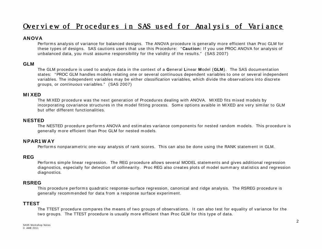
Overview of Procedures in SAS used for Analysis of Variance

ANOVA Performs analysis of variance for balanced designs. The ANOVA procedure is generally more efficient than Proc GLM for these types of designs. SAS cautions users that use this Procedure: “Caution: If you use PROC ANOVA for analysis of unbalanced data, you must assume responsibility for the validity of the results.” (SAS 2007)

GLM

The GLM procedure is used to analyze data in the context of a General Linear Model (GLM). The SAS documentation states: “PROC GLM handles models relating one or several continuous dependent variables to one or several independent variables. The independent variables may be either classification variables, which divide the observations into discrete groups, or continuous variables.” (SAS 2007)

MIXED

The MIXED procedure was the next generation of Procedures dealing with ANOVA. MIXED fits mixed models by incorporating covariance structures in the model fitting process. Some options avaible in MIXED are very similar to GLM but offer different functionalities.

NESTED

The NESTED procedure performs ANOVA and estimates variance components for nested random models. This procedure is generally more efficient than Proc GLM for nested models.

NPAR1WAY Performs nonparametric one-way analysis of rank scores. This can also be done using the RANK statement in GLM. REG

Performs simple linear regression. The REG procedure allows several MODEL statements and gives additional regression diagnostics, especially for detection of collinearity. Proc REG also creates plots of model summary statistics and regression diagnostics.

RSREG

This procedure performs quadratic response-surface regression, canonical and ridge analysis. The RSREG procedure is generally recommended for data from a response surface experiment.

TTEST

The TTEST procedure compares the means of two groups of observations. It can also test for equality of variance for the two groups. The TTEST procedure is usually more efficient than Proc GLM for this type of data.


VARCOMP Estimates variance components for a general linear model. For more advanced models there are a number of Procedures available today. Take a look at the SAS online documentation available at: http://support.sas.com/onlinedoc/913/docMainpage.jsp for more information

http://support.sas.com/onlinedoc/913/docMainpage.jsp


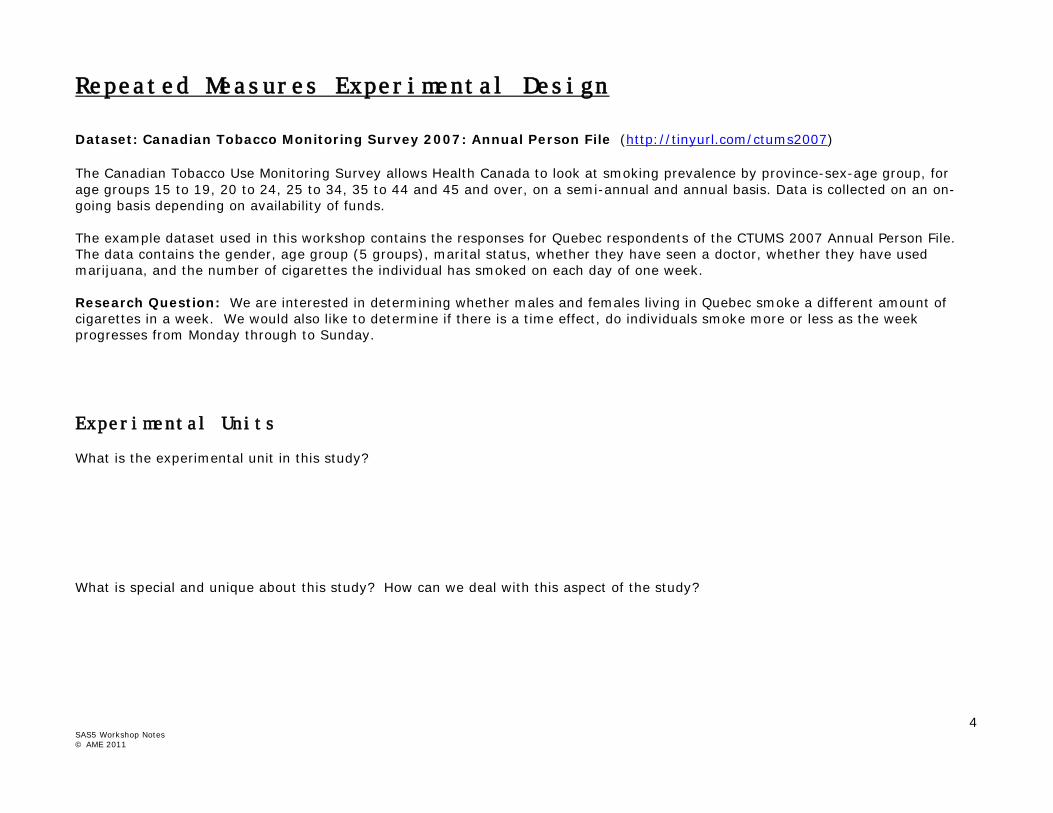
Repeated Measures Experimental Design

Dataset: Canadian Tobacco Monitoring Survey 2007: Annual Person File (http://tinyurl.com/ctums2007) The Canadian Tobacco Use Monitoring Survey allows Health Canada to look at smoking prevalence by province-sex-age group, for age groups 15 to 19, 20 to 24, 25 to 34, 35 to 44 and 45 and over, on a semi-annual and annual basis. Data is collected on an on-going basis depending on availability of funds. The example dataset used in this workshop contains the responses for Quebec respondents of the CTUMS 2007 Annual Person File. The data contains the gender, age group (5 groups), marital status, whether they have seen a doctor, whether they have used marijuana, and the number of cigarettes the individual has smoked on each day of one week. Research Question: We are interested in determining whether males and females living in Quebec smoke a different amount of cigarettes in a week. We would also like to determine if there is a time effect, do individuals smoke more or less as the week progresses from Monday through to Sunday.

Experimental Units

What is the experimental unit in this study? What is special and unique about this study? How can we deal with this aspect of the study?

http://tinyurl.com/ctums2007


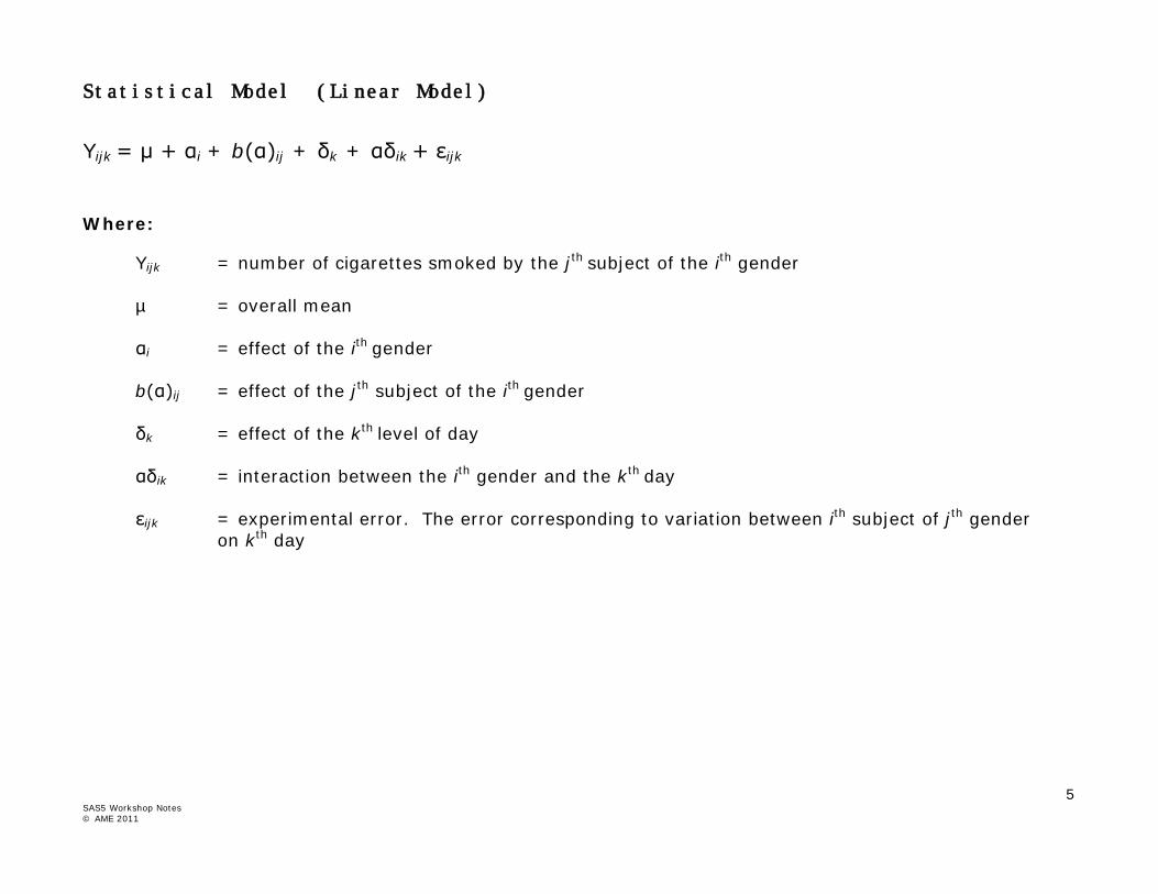
Statistical Model (Linear Model)

Yijk = µ + αi + b(α)ij + δk + αδik + εijk Where:

Yijk = number of cigarettes smoked by the jth subject of the ith gender µ = overall mean αi = effect of the ith gender b(α)ij = effect of the jth subject of the ith gender δk = effect of the kth level of day αδik = interaction between the ith gender and the kth day εijk = experimental error. The error corresponding to variation between ith subject of jth gender

on kth day


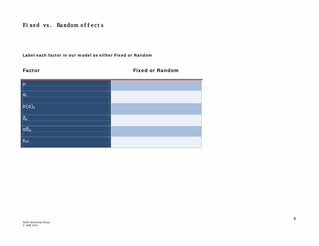
Fixed vs. Random effects

Label each factor in our model as either Fixed or Random Factor

Fixed or Random

µ

αi

b(α)ij

δk

αδik

εijk


Three ways to look at a Repeated Measures Experimental Design

1. Split-plot design

2. Multivariate repeated measures design using Proc GLM

3. Multivariate repeated measures design using Proc MIXED

One of the tricks to running a repeated measures design is the format of the data. The data must be created in a multivariate format for 2. – one line for each individual. For 1. and 3. the data must be created in a univariate format – with one line per observation per individual. Multivariate format: Obs Subject AGEGRP5 SEX DVMARST day1 day2 day3 day4 day5 day6 1 3 25-34 years Female Single 8 8 8 8 8 8 2 40 15-19 years Female Common-law/Married 10 10 10 10 10 10 3 117 15-19 years Female Single 6 6 6 6 6 10 4 139 15-19 years Female Single 20 20 20 20 20 20 5 166 45 years & over Male Common-law/Married 0 2 1 2 1 2 Univariate format: Obs Subject AGEGRP5 SEX DVMARST smoking day 1 3 25-34 years Female Single 8 1 2 3 25-34 years Female Single 8 2 3 3 25-34 years Female Single 8 3 4 3 25-34 years Female Single 8 4 5 3 25-34 years Female Single 8 5 6 3 25-34 years Female Single 8 6 7 3 25-34 years Female Single 8 7 8 40 15-19 years Female Common-law/Married 10 1


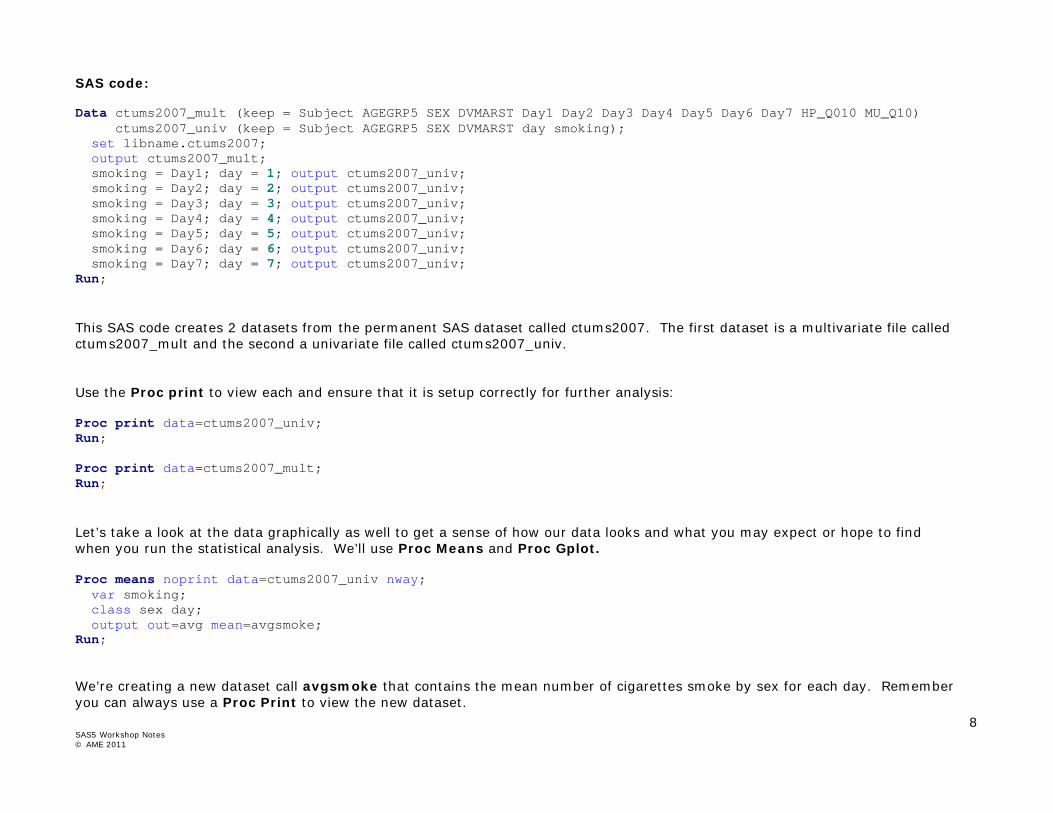
SAS code: Data ctums2007_mult (keep = Subject AGEGRP5 SEX DVMARST Day1 Day2 Day3 Day4 Day5 Day6 Day7 HP_Q010 MU_Q10) ctums2007_univ (keep = Subject AGEGRP5 SEX DVMARST day smoking); set libname.ctums2007; output ctums2007_mult; smoking = Day1; day = 1; output ctums2007_univ; smoking = Day2; day = 2; output ctums2007_univ; smoking = Day3; day = 3; output ctums2007_univ; smoking = Day4; day = 4; output ctums2007_univ; smoking = Day5; day = 5; output ctums2007_univ; smoking = Day6; day = 6; output ctums2007_univ; smoking = Day7; day = 7; output ctums2007_univ; Run; This SAS code creates 2 datasets from the permanent SAS dataset called ctums2007. The first dataset is a multivariate file called ctums2007_mult and the second a univariate file called ctums2007_univ. Use the Proc print to view each and ensure that it is setup correctly for further analysis: Proc print data=ctums2007_univ; Run; Proc print data=ctums2007_mult; Run; Let’s take a look at the data graphically as well to get a sense of how our data looks and what you may expect or hope to find when you run the statistical analysis. We’ll use Proc Means and Proc Gplot. Proc means noprint data=ctums2007_univ nway; var smoking; class sex day; output out=avg mean=avgsmoke; Run; We’re creating a new dataset call avgsmoke that contains the mean number of cigarettes smoke by sex for each day. Remember you can always use a Proc Print to view the new dataset.


Proc gplot data=avg; plot avgsmoke*day=sex / haxis=0 to 8 by 1 hminor=0 vminor=0; symbol1 v=star c=black i=join l=1; symbol2 v=plus c=black i=join l=2; title "Average number of cigarettes smoked per day by Gender"; Run; Quit; Proc Gplot will open a new Graph window with the resulting plots. What do you see in the plots? What do you expect when you run the analysis of variance? A difference between genders? A difference between days? 1. SAS code for Split-plot design

/* Using PROC GLM - Split-plot design with Sex as the Main Plot and Time as the Subplot */ Proc glm data=ctums2007_univ; class sex day subject; model smoking = sex subject(sex) day sex*day; test h=sex e=subject(sex); Run; Note: The model statement contains the entire “translated” model from p.29. We use a test statement to specify the correct error term for our Main plot – which is sex in our example.


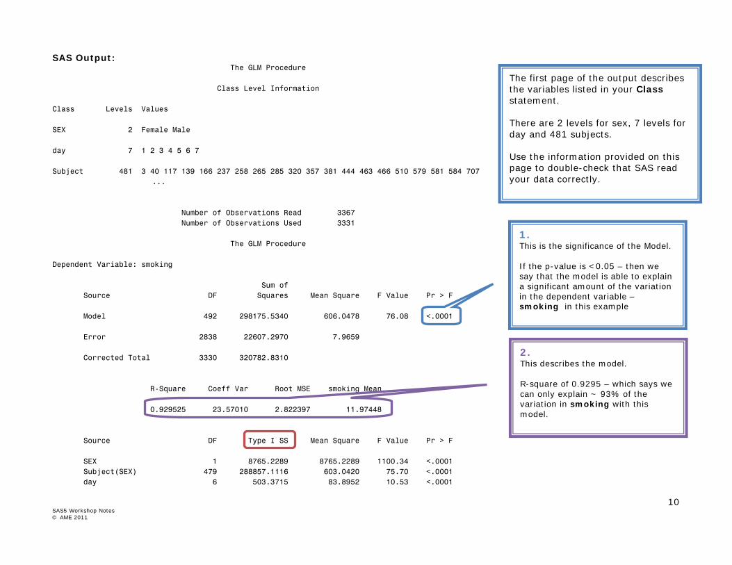
SAS Output: The GLM Procedure Class Level Information Class Levels Values SEX 2 Female Male day 7 1 2 3 4 5 6 7 Subject 481 3 40 117 139 166 237 258 265 285 320 357 381 444 463 466 510 579 581 584 707 ... Number of Observations Read 3367 Number of Observations Used 3331 The GLM Procedure Dependent Variable: smoking Sum of Source DF Squares Mean Square F Value Pr > F Model 492 298175.5340 606.0478 76.08 <.0001 Error 2838 22607.2970 7.9659 Corrected Total 3330 320782.8310 R-Square Coeff Var Root MSE smoking Mean 0.929525 23.57010 2.822397 11.97448 Source DF Type I SS Mean Square F Value Pr > F SEX 1 8765.2289 8765.2289 1100.34 <.0001 Subject(SEX) 479 288857.1116 603.0420 75.70 <.0001 day 6 503.3715 83.8952 10.53 <.0001

The first page of the output describes the variables listed in your Class statement. There are 2 levels for sex, 7 levels for day and 481 subjects. Use the information provided on this page to double-check that SAS read your data correctly.

1. This is the significance of the Model. If the p-value is <0.05 – then we say that the model is able to explain a significant amount of the variation in the dependent variable – smoking in this example

2. This describes the model. R-square of 0.9295 – which says we can only explain ~ 93% of the variation in smoking with this model.


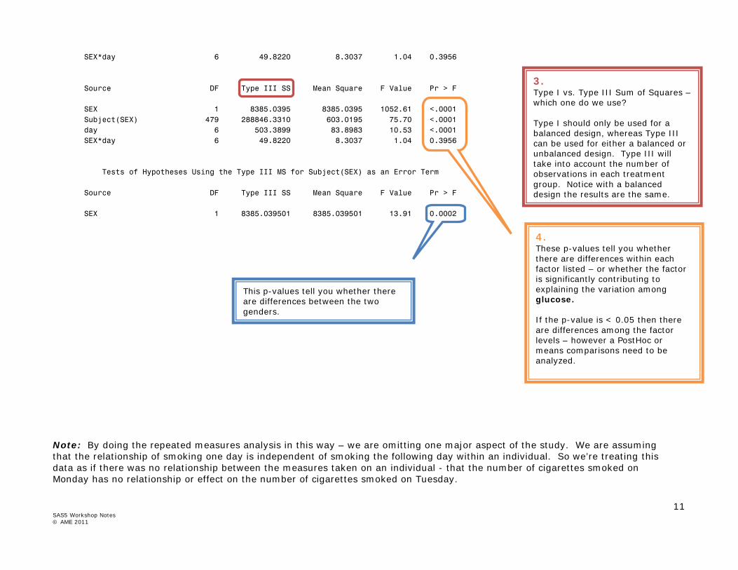
SEX*day 6 49.8220 8.3037 1.04 0.3956 Source DF Type III SS Mean Square F Value Pr > F SEX 1 8385.0395 8385.0395 1052.61 <.0001 Subject(SEX) 479 288846.3310 603.0195 75.70 <.0001 day 6 503.3899 83.8983 10.53 <.0001 SEX*day 6 49.8220 8.3037 1.04 0.3956 Tests of Hypotheses Using the Type III MS for Subject(SEX) as an Error Term Source DF Type III SS Mean Square F Value Pr > F SEX 1 8385.039501 8385.039501 13.91 0.0002 Note: By doing the repeated measures analysis in this way – we are omitting one major aspect of the study. We are assuming that the relationship of smoking one day is independent of smoking the following day within an individual. So we’re treating this data as if there was no relationship between the measures taken on an individual - that the number of cigarettes smoked on Monday has no relationship or effect on the number of cigarettes smoked on Tuesday.

3. Type I vs. Type III Sum of Squares – which one do we use? Type I should only be used for a balanced design, whereas Type III can be used for either a balanced or unbalanced design. Type III will take into account the number of observations in each treatment group. Notice with a balanced design the results are the same.

4. These p-values tell you whether there are differences within each factor listed – or whether the factor is significantly contributing to explaining the variation among glucose. If the p-value is < 0.05 then there are differences among the factor levels – however a PostHoc or means comparisons need to be analyzed.

This p-values tell you whether there are differences between the two genders.


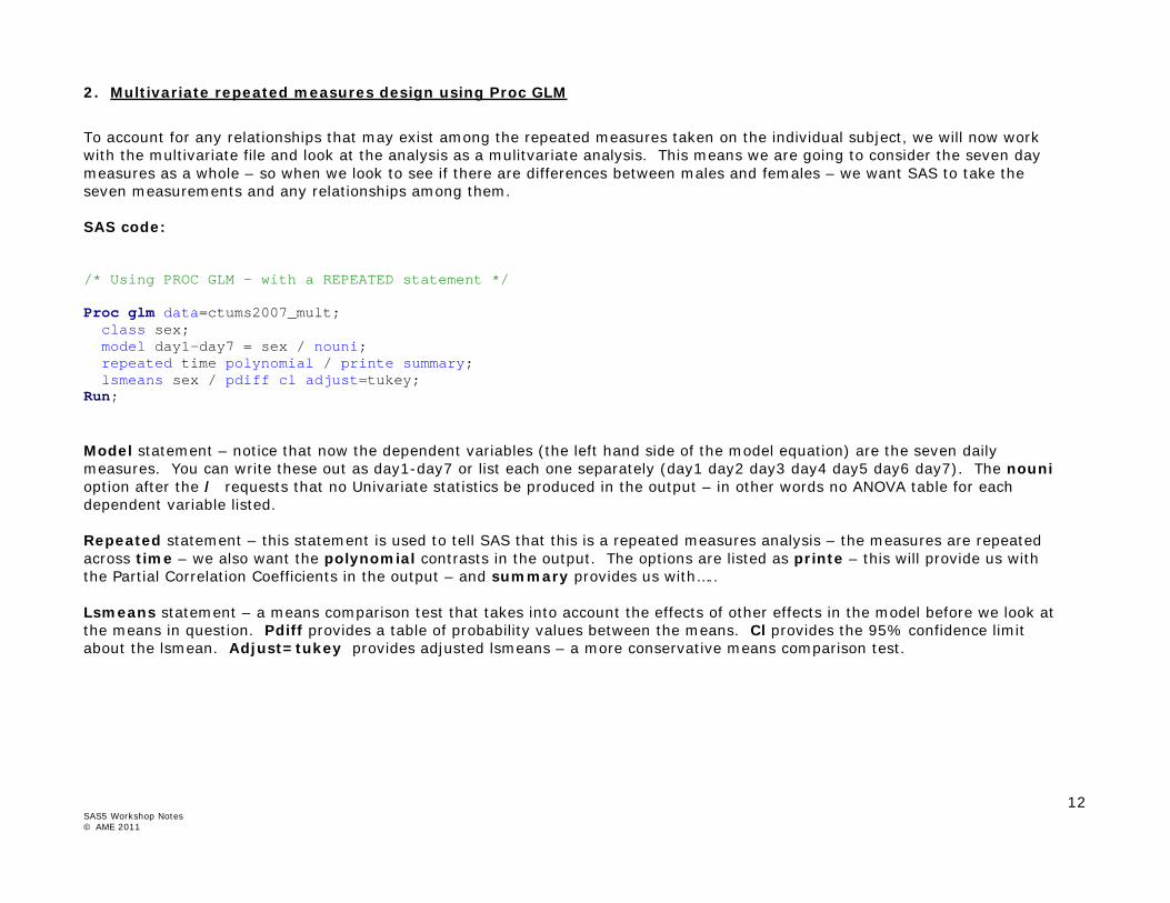
2. Multivariate repeated measures design using Proc GLM

To account for any relationships that may exist among the repeated measures taken on the individual subject, we will now work with the multivariate file and look at the analysis as a mulitvariate analysis. This means we are going to consider the seven day measures as a whole – so when we look to see if there are differences between males and females – we want SAS to take the seven measurements and any relationships among them. SAS code: /* Using PROC GLM - with a REPEATED statement */ Proc glm data=ctums2007_mult; class sex; model day1-day7 = sex / nouni; repeated time polynomial / printe summary; lsmeans sex / pdiff cl adjust=tukey; Run; Model statement – notice that now the dependent variables (the left hand side of the model equation) are the seven daily measures. You can write these out as day1-day7 or list each one separately (day1 day2 day3 day4 day5 day6 day7). The nouni option after the / requests that no Univariate statistics be produced in the output – in other words no ANOVA table for each dependent variable listed. Repeated statement – this statement is used to tell SAS that this is a repeated measures analysis – the measures are repeated across time – we also want the polynomial contrasts in the output. The options are listed as printe – this will provide us with the Partial Correlation Coefficients in the output – and summary provides us with….. Lsmeans statement – a means comparison test that takes into account the effects of other effects in the model before we look at the means in question. Pdiff provides a table of probability values between the means. Cl provides the 95% confidence limit about the lsmean. Adjust=tukey provides adjusted lsmeans – a more conservative means comparison test.


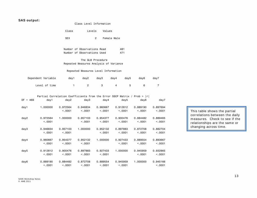
SAS output: Class Level Information Class Levels Values SEX 2 Female Male Number of Observations Read 481 Number of Observations Used 471 The GLM Procedure Repeated Measures Analysis of Variance Repeated Measures Level Information Dependent Variable day1 day2 day3 day4 day5 day6 day7 Level of time 1 2 3 4 5 6 7 Partial Correlation Coefficients from the Error SSCP Matrix / Prob > |r| DF = 469 day1 day2 day3 day4 day5 day6 day7 day1 1.000000 0.972564 0.946834 0.960667 0.912812 0.889190 0.897694 <.0001 <.0001 <.0001 <.0001 <.0001 <.0001 day2 0.972564 1.000000 0.957103 0.954377 0.900476 0.884482 0.889465 <.0001 <.0001 <.0001 <.0001 <.0001 <.0001 day3 0.946834 0.957103 1.000000 0.952132 0.897883 0.872708 0.882704 <.0001 <.0001 <.0001 <.0001 <.0001 <.0001 day4 0.960667 0.954377 0.952132 1.000000 0.927433 0.889554 0.893667 <.0001 <.0001 <.0001 <.0001 <.0001 <.0001 day5 0.912812 0.900476 0.897883 0.927433 1.000000 0.945959 0.932865 <.0001 <.0001 <.0001 <.0001 <.0001 <.0001 day6 0.889190 0.884482 0.872708 0.889554 0.945959 1.000000 0.945166 <.0001 <.0001 <.0001 <.0001 <.0001 <.0001

This table shows the partial correlations between the daily measures. Check to see if the relationships are the same or changing across time.


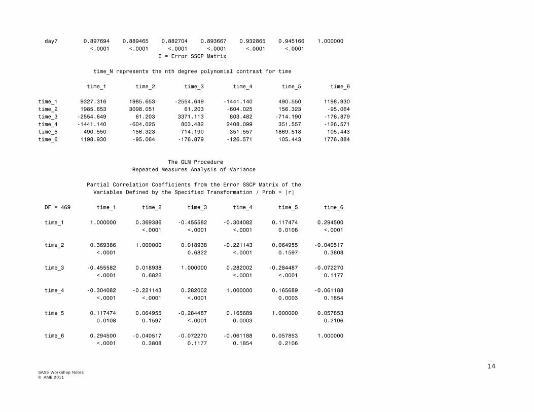
day7 0.897694 0.889465 0.882704 0.893667 0.932865 0.945166 1.000000 <.0001 <.0001 <.0001 <.0001 <.0001 <.0001 E = Error SSCP Matrix time_N represents the nth degree polynomial contrast for time time_1 time_2 time_3 time_4 time_5 time_6 time_1 9327.316 1985.653 -2554.649 -1441.140 490.550 1198.930 time_2 1985.653 3098.051 61.203 -604.025 156.323 -95.064 time_3 -2554.649 61.203 3371.113 803.482 -714.190 -176.879 time_4 -1441.140 -604.025 803.482 2408.099 351.557 -126.571 time_5 490.550 156.323 -714.190 351.557 1869.518 105.443 time_6 1198.930 -95.064 -176.879 -126.571 105.443 1776.884 The GLM Procedure Repeated Measures Analysis of Variance Partial Correlation Coefficients from the Error SSCP Matrix of the Variables Defined by the Specified Transformation / Prob > |r| DF = 469 time_1 time_2 time_3 time_4 time_5 time_6 time_1 1.000000 0.369386 -0.455582 -0.304082 0.117474 0.294500 <.0001 <.0001 <.0001 0.0108 <.0001 time_2 0.369386 1.000000 0.018938 -0.221143 0.064955 -0.040517 <.0001 0.6822 <.0001 0.1597 0.3808 time_3 -0.455582 0.018938 1.000000 0.282002 -0.284487 -0.072270 <.0001 0.6822 <.0001 <.0001 0.1177 time_4 -0.304082 -0.221143 0.282002 1.000000 0.165689 -0.061188 <.0001 <.0001 <.0001 0.0003 0.1854 time_5 0.117474 0.064955 -0.284487 0.165689 1.000000 0.057853 0.0108 0.1597 <.0001 0.0003 0.2106 time_6 0.294500 -0.040517 -0.072270 -0.061188 0.057853 1.000000 <.0001 0.3808 0.1177 0.1854 0.2106


Sphericity Tests Mauchly's Variables DF Criterion Chi-Square Pr > ChiSq Transformed Variates 20 0.1351514 934.19028 <.0001 Orthogonal Components 20 0.1351514 934.19028 <.0001 MANOVA Test Criteria and Exact F Statistics for the Hypothesis of no time Effect H = Type III SSCP Matrix for time E = Error SSCP Matrix S=1 M=2 N=231 Statistic Value F Value Num DF Den DF Pr > F Wilks' Lambda 0.93725336 5.18 6 464 <.0001 Pillai's Trace 0.06274664 5.18 6 464 <.0001 Hotelling-Lawley Trace 0.06694736 5.18 6 464 <.0001 Roy's Greatest Root 0.06694736 5.18 6 464 <.0001 MANOVA Test Criteria and Exact F Statistics for the Hypothesis of no time*SEX Effect H = Type III SSCP Matrix for time*SEX E = Error SSCP Matrix S=1 M=2 N=231 Statistic Value F Value Num DF Den DF Pr > F Wilks' Lambda 0.97905681 1.65 6 464 0.1305 Pillai's Trace 0.02094319 1.65 6 464 0.1305 Hotelling-Lawley Trace 0.02139119 1.65 6 464 0.1305 Roy's Greatest Root 0.02139119 1.65 6 464 0.1305

Sphericity tests check to see if the relationships among the daily measures are an Identity matrix – which means there are no relationships among the daily measures. A p-value < 0.05 suggests that you reject the null hypothesis and that there are indeed relationships among your daily measures.

1. SAS provides you with 4 test results – choose one and stick with it. For this workshop we will use the Wilks’ Lambda statistic.

2. Read the Hypothesis statement to understand the results presented in the table. In this case – we’re looking at the effect of Time. A p-value < 0.05 – we reject the Null hypothesis – and state that there is a time effect.

3. Read the Hypothesis statement to understand the results presented in the table. In this case – we’re looking at the effect of Time*sex. A p-value > 0.05 – we accept the Null hypothesis – and state that there is no difference between males and females across time.


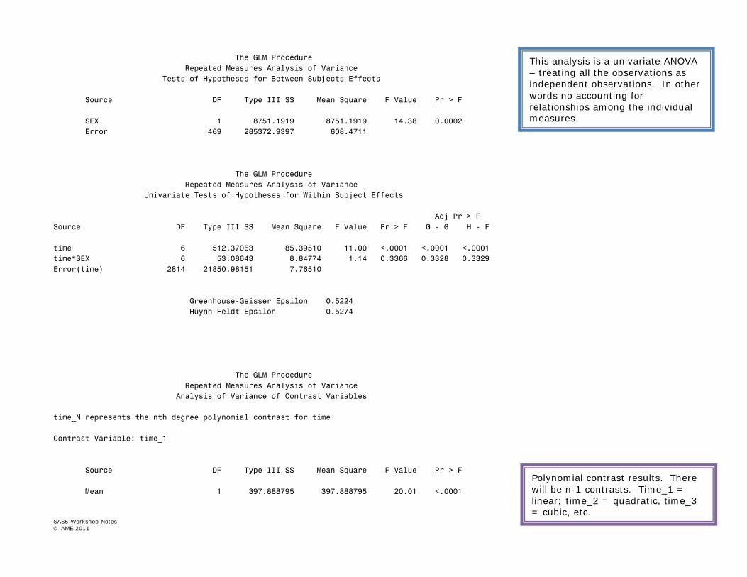
The GLM Procedure Repeated Measures Analysis of Variance Tests of Hypotheses for Between Subjects Effects Source DF Type III SS Mean Square F Value Pr > F SEX 1 8751.1919 8751.1919 14.38 0.0002 Error 469 285372.9397 608.4711 The GLM Procedure Repeated Measures Analysis of Variance Univariate Tests of Hypotheses for Within Subject Effects Adj Pr > F Source DF Type III SS Mean Square F Value Pr > F G - G H - F time 6 512.37063 85.39510 11.00 <.0001 <.0001 <.0001 time*SEX 6 53.08643 8.84774 1.14 0.3366 0.3328 0.3329 Error(time) 2814 21850.98151 7.76510 Greenhouse-Geisser Epsilon 0.5224 Huynh-Feldt Epsilon 0.5274 The GLM Procedure Repeated Measures Analysis of Variance Analysis of Variance of Contrast Variables time_N represents the nth degree polynomial contrast for time Contrast Variable: time_1 Source DF Type III SS Mean Square F Value Pr > F Mean 1 397.888795 397.888795 20.01 <.0001

This analysis is a univariate ANOVA – treating all the observations as independent observations. In other words no accounting for relationships among the individual measures.

Polynomial contrast results. There will be n-1 contrasts. Time_1 = linear; time_2 = quadratic, time_3 = cubic, etc.


SEX 1 1.374388 1.374388 0.07 0.7928 Error 469 9327.316392 19.887668 Contrast Variable: time_2 Source DF Type III SS Mean Square F Value Pr > F Mean 1 1.432255 1.432255 0.22 0.6417 SEX 1 26.019657 26.019657 3.94 0.0478 Error 469 3098.050760 6.605652 The GLM Procedure Least Squares Means Adjustment for Multiple Comparisons: Tukey-Kramer H0:LSMean1= LSMean2 SEX day1 LSMEAN Pr > |t| Female 10.0813008 0.0002 Male 13.2844444 SEX day1 LSMEAN 95% Confidence Limits Female 10.081301 8.909690 11.252911 Male 13.284444 12.059378 14.509511 Least Squares Means for Effect SEX Difference Simultaneous 95% Between Confidence Limits for i j Means LSMean(i)-LSMean(j) 1 2 -3.203144 -4.898272 -1.508015

Lsmeans results


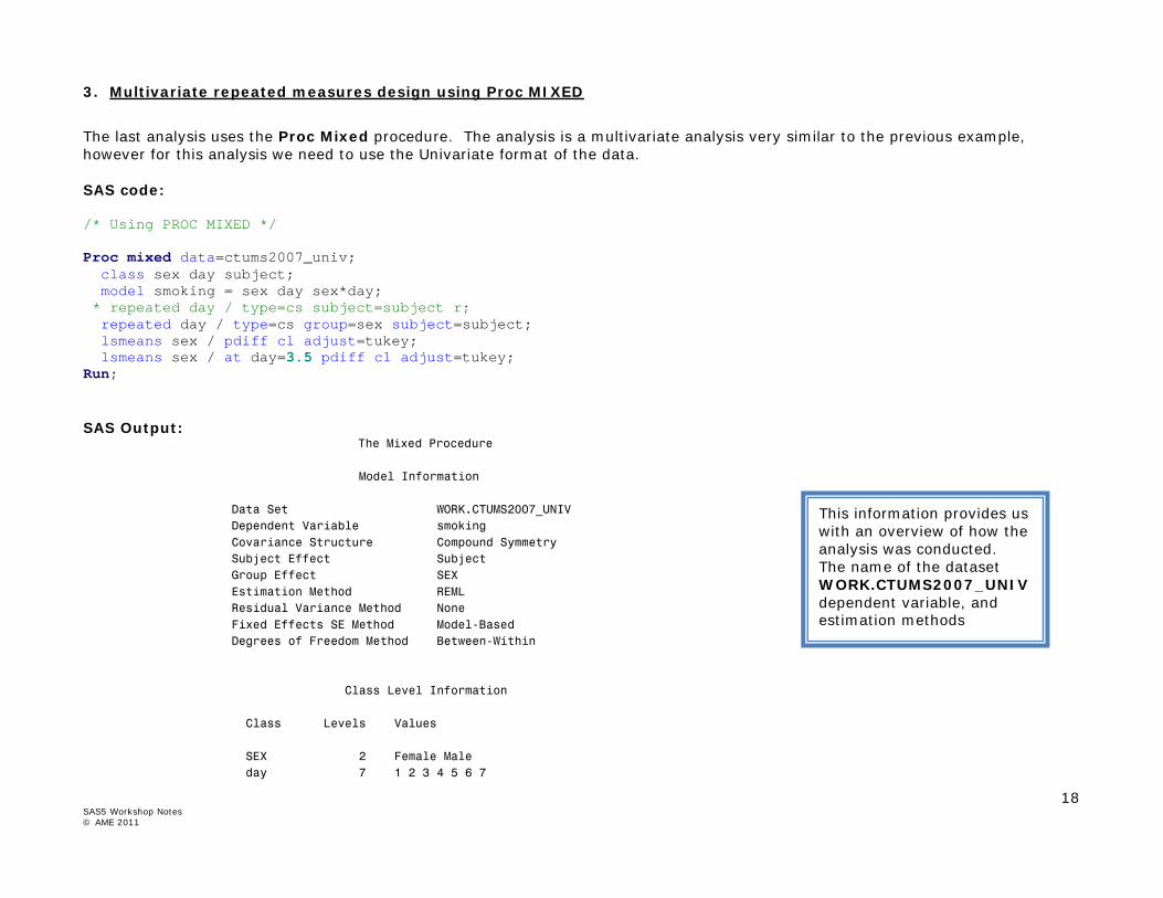
3. Multivariate repeated measures design using Proc MIXED

The last analysis uses the Proc Mixed procedure. The analysis is a multivariate analysis very similar to the previous example, however for this analysis we need to use the Univariate format of the data. SAS code: /* Using PROC MIXED */ Proc mixed data=ctums2007_univ; class sex day subject; model smoking = sex day sex*day; * repeated day / type=cs subject=subject r; repeated day / type=cs group=sex subject=subject; lsmeans sex / pdiff cl adjust=tukey; lsmeans sex / at day=3.5 pdiff cl adjust=tukey; Run; SAS Output:

The Mixed Procedure Model Information Data Set WORK.CTUMS2007_UNIV Dependent Variable smoking Covariance Structure Compound Symmetry Subject Effect Subject Group Effect SEX Estimation Method REML Residual Variance Method None Fixed Effects SE Method Model-Based Degrees of Freedom Method Between-Within Class Level Information Class Levels Values SEX 2 Female Male day 7 1 2 3 4 5 6 7

This information provides us with an overview of how the analysis was conducted. The name of the dataset WORK.CTUMS2007_UNIV dependent variable, and estimation methods


Class Level Information Class Levels Values Subject 481 3 40 117 139 166 237 258 265 285 320 357 381 444 463 466 510 579 581 584 707 711 791 Dimensions Covariance Parameters 4 Columns in X 24 Columns in Z 0 Subjects 481 Max Obs Per Subject 7 Number of Observations Number of Observations Read 3367 Number of Observations Used 3331 Number of Observations Not Used 36 Iteration History Iteration Evaluations -2 Res Log Like Criterion 0 1 24556.27159282 1 2 18436.77349240 0.00000293 2 1 18436.75526689 0.00000000 Convergence criteria met. Covariance Parameter Estimates Cov Parm Subject Group Estimate Variance Subject SEX Female 8.3789 CS Subject SEX Female 74.1964 Variance Subject SEX Male 7.5118 CS Subject SEX Male 100.36

Similar to the Proc glm output this part of the output describes the variables listed in your Class statement.

Information about the matrices used in the analysis

Iteration history – remember Proc mixed uses an iterative approach to te analysis. Covariance Parameter Estimates – provides estimates of the random effects included in your model


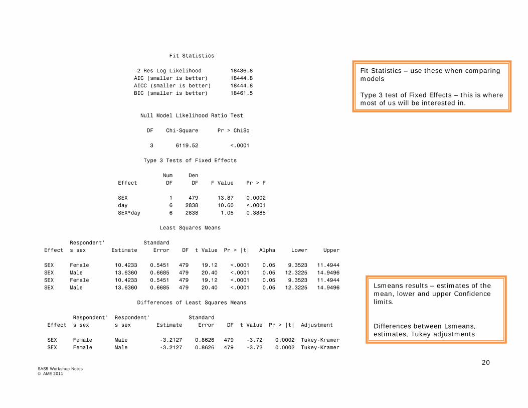
Fit Statistics -2 Res Log Likelihood 18436.8 AIC (smaller is better) 18444.8 AICC (smaller is better) 18444.8 BIC (smaller is better) 18461.5 Null Model Likelihood Ratio Test DF Chi-Square Pr > ChiSq 3 6119.52 <.0001 Type 3 Tests of Fixed Effects Num Den Effect DF DF F Value Pr > F SEX 1 479 13.87 0.0002 day 6 2838 10.60 <.0001 SEX*day 6 2838 1.05 0.3885 Least Squares Means Respondent' Standard Effect s sex Estimate Error DF t Value Pr > |t| Alpha Lower Upper SEX Female 10.4233 0.5451 479 19.12 <.0001 0.05 9.3523 11.4944 SEX Male 13.6360 0.6685 479 20.40 <.0001 0.05 12.3225 14.9496 SEX Female 10.4233 0.5451 479 19.12 <.0001 0.05 9.3523 11.4944 SEX Male 13.6360 0.6685 479 20.40 <.0001 0.05 12.3225 14.9496 Differences of Least Squares Means Respondent' Respondent' Standard Effect s sex s sex Estimate Error DF t Value Pr > |t| Adjustment SEX Female Male -3.2127 0.8626 479 -3.72 0.0002 Tukey-Kramer SEX Female Male -3.2127 0.8626 479 -3.72 0.0002 Tukey-Kramer

Fit Statistics – use these when comparing models Type 3 test of Fixed Effects – this is where most of us will be interested in.

Lsmeans results – estimates of the mean, lower and upper Confidence limits. Differences between Lsmeans, estimates, Tukey adjustments


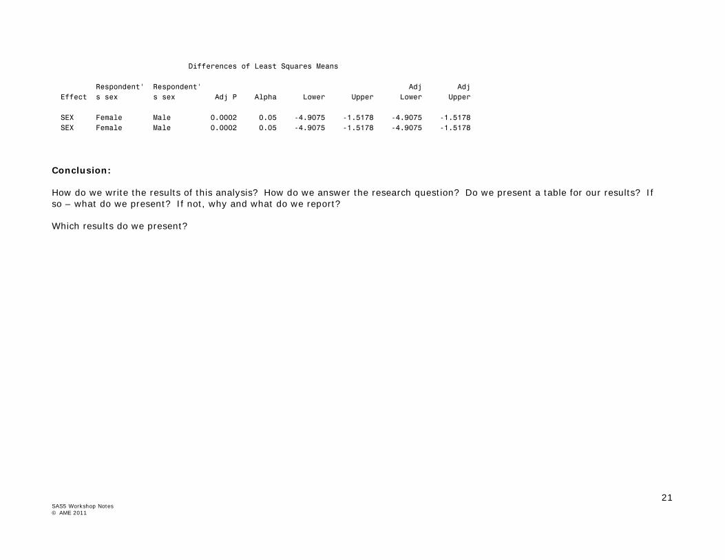
Differences of Least Squares Means Respondent' Respondent' Adj Adj Effect s sex s sex Adj P Alpha Lower Upper Lower Upper SEX Female Male 0.0002 0.05 -4.9075 -1.5178 -4.9075 -1.5178 SEX Female Male 0.0002 0.05 -4.9075 -1.5178 -4.9075 -1.5178 Conclusion: How do we write the results of this analysis? How do we answer the research question? Do we present a table for our results? If so – what do we present? If not, why and what do we report? Which results do we present?

sas5 repeated measures experimental design · multivariate repeated measures design using proc...

Documents