sap press - abap development for sap netweaver bi user exits and badls (3ed)
DESCRIPTION
SAP Press - ABAP Development for SAP NetWeaver BI User Exits and BAdls (3ed)TRANSCRIPT


SAP® EssentialsExpert SAP knowledge for your day-to-day work
Whether you wish to expand your SAP knowledge, deepen it, or master a use case, SAP Essentials provide you with targeted expert knowledge that helps sup-port you in your day-to-day work. To the point, detailed, and ready to use.
SAP PRESS is a joint initiative of SAP and Galileo Press. The know-how offered by SAP specialists combined with the expertise of the Galileo Press publishing house offers the reader expert books in the field. SAP PRESS features first-hand informa-tion and expert advice, and provides useful skills for professional decision-making.
SAP PRESS offers a variety of books on technical and business related topics for the SAP user. For further information, please visit our website: http://www.sap-press.com.
David Haslam and Puneet Asthana SAP Certified Development Associate—ABAP with SAP NetWeaver 7.02 (2nd Edition) 2012, 630 pp., paperback ISBN 978-1-59229-435-0
Rich Heilman and Thomas Jung (2nd Edition) Next Generation ABAP Development 2011, 735 pp., hardcover ISBN 978-1-59229-352-0
Sergey Korolev ABAP Development for Financial Accounting: Custom Enhancements 2011, 252 pp., hardcover ISBN 978-1-59229-370-4
Ilja-Daniel Werner ABAP Development for SAP Business Workflow 2012, 194 pp., hardcover ISBN 978-1-59229-394-0

Dirk Herzog
ABAP® Development for SAP NetWeaver® BW
Exits, BAdIs, and Enhancements
Bonn � Boston
Dear Reader,
Maybe you’ve seen this book before—perhaps being shared among colleagues, within easy reach in a peer’s office, or even on your own bookshelf. Since its first publication in 2006, it has been one of our most successful development books, prompting our editorial team to pursue yet another updated edition.
As its third English-edition editor, I have a hunch about what makes this book so popular with readers: Dirk Herzog simply knows how to teach ABAP. His ABAP development books successfully blend industry expertise with high-impact lessons that both educate and empower readers. As the co-author and course instructor of “User Exits in SAP BW,” Dirk knows how to equip users with the information they need to maximize SAP NetWeaver BW systems. His practical examples of custom code—framed by thoughtful comments that will lead you through custom develop-ment—will help you connect the dots and apply best practices to your own work. Further, Dirk’s active contributions to the SAP Community Network and ongoing role as a topic expert enable him to share the most up-to-date techniques and real-world examples with his students and colleagues. With the purchase of this book as a resource for custom enhancements, you have become another beneficiary of his expertise.
And so I feel confident that this edition, like its predecessors, will deliver valuable exposure to standard custom developments for SAP NetWeaver BW implemen-tations. Because we appreciate your business, we welcome your feedback. Your comments and suggestions are the most useful tools to help us improve our books for you, the reader, even as experts like Dirk both shape and adapt to the changes that mark the business intelligence world. We encourage you to visit our website at www.sap-press.com and share your feedback about the third edition of ABAP Devel-
opment for SAP NetWeaver BW. Thank you for purchasing a book from SAP PRESS!
Emily Nicholls Editor, SAP PRESS
Galileo Press Boston, MA
http://www.sap-press.com

Notes on Usage
This e-book is protected by copyright. By purchasing this e-book, you have agreed to accept and adhere to the copyrights. You are entitled to use this e-book for personal purposes. You may print and copy it, too, but also only for personal use. Sharing an electronic or printed copy with others, however, is not permitted, neither as a whole nor in parts. Of course, making them available on the Internet or in a company network is illegal as well.
For detailed and legally binding usage conditions, please refer to the section Legal Notes.
This e-book copy contains a digital watermark, a signature that indicates which person may use this copy:

Imprint
This e-book is a publication many contributed to, specifically:
Editor Janina SchweitzerEnglish Edition Editor Emily NichollsTranslation Lemoine International, Inc., Salt Lake City, UTCopyeditor Pamela SiskaCover Design Nadine Kohl, Graham GearyPhoto Credit iStock, 4721596, Mahalingam SankararamanProduction E-Book Kelly O’CallaghanTypesetting E-Book Publishers’ Design and Production Services, Inc.
We hope that you liked this e-book. Please share your feedback with us and read the Service Pages to find out how to contact us.
The Library of Congress has cataloged the printed edition as follows:Herzog, Dirk.
[ABAP—programmierung für SAP NetWeaver BI. English]
ABAP development for SAP NetWeaver BW : exits, BAdIs, and enhancements /Dirk Herzog. — 3rd
edition. pages cm
Translation of: ABAP—programmierung für SAP NetWeaver BW.
Rev. ed. of: ABAP development for SAP NetWeaver BI : user exits and BAdIs, and originally pub-
lished in German under the title:
ABAP—programmierung für SAP NetWeaver BI : user Exits und BAdIs.
ISBN 978-1-59229-424-4 — ISBN 1-59229-424-3 1. Data warehousing. 2. SAP NetWeaver BW.
3. ABAP/4 (Computer program
language) 4. Business—Databases. I. Title.
QA76.9.D37H475 2013
005.74’5—dc23
2012026605
ISBN 978-1-59229-424-4 (print) ISBN 978-1-59229-829-7 (e-book) ISBN 978-1-59229-830-3 (print and e-book)
© 2012 by Galileo Press Inc., Boston (MA) 3rd edition 2012 3rd German edition published 2012 by Galileo Press, Bonn, Germany

7
Contents
Preface to the 3rd Edition .......................................................................... 11Introduction ............................................................................................... 13
1 Performance .............................................................................. 17
1.1 Table Types in ABAP ................................................................... 171.2 Loops and Read Accesses to Tables ............................................. 201.3 Field Symbols ............................................................................. 221.4 Database Accesses and Cache ..................................................... 24
2 User Exits and BAdIs in the Extraction Process ....................... 27
2.1 Usage Options ............................................................................ 272.2 Generic Extractors ....................................................................... 282.3 User Exit RSAP0001 .................................................................... 33
2.3.1 How to Use the Exit ....................................................... 342.3.2 Structured Composition of the ZXRSAU01 Include ......... 362.3.3 Implementing User Exit EXIT_SAPLRSAP_001 for
Currency Extraction ........................................................ 412.3.4 Using the Hierarchy Exit ................................................. 432.3.5 Surrogate for the Generic Hierarchy Extractor ................. 452.3.6 Transferring Parameters to the User Exit ......................... 46
2.4 BAdI RSU5_SAPI_BADI ............................................................... 472.4.1 Methods ........................................................................ 472.4.2 Advantages and Disadvantages ....................................... 48
3 User Exits in Data Import Processes ........................................ 51
3.1 Transformation ............................................................................ 513.1.1 Deriving Characteristics .................................................. 543.1.2 Deriving Key Figures ...................................................... 583.1.3 Start Routine in the Transformation ................................ 633.1.4 End Routine in the Transformation ................................. 683.1.5 Expert Routine in the Transformation ............................. 71
3.2 Routines in the Data Transfer Process .......................................... 81

8
Contents
3.2.1 Selecting a File Name in the Data Transfer Process ......... 813.2.2 Determining a Characteristic Value Selection in
the Data Transfer Process ............................................... 833.3 Importing a Hierarchy from an Unstructured Microsoft
Excel Sheet ................................................................................. 863.3.1 Creating the DataStore Object ........................................ 883.3.2 Creating the DataSource ................................................. 893.3.3 Creating the Transformation ........................................... 913.3.4 Creating the Start Routine .............................................. 923.3.5 Creating the End Routine ............................................... 943.3.6 Creating a Data Transfer Process ..................................... 1033.3.7 Creating a Query ............................................................ 1053.3.8 Implementation in SAP BW 3.x ...................................... 105
3.4 Recommendations for SAP NetWeaver 7.3 .................................. 106
4 User Exits and BAdls in Reporting ........................................... 107
4.1 Variable Exit RSR00001 .............................................................. 1074.1.1 Interface of Function Module EXIT_SAPLRSR0_001 ....... 1094.1.2 Implementation for I_STEP = 1 ....................................... 1134.1.3 Implementation for I_STEP = 2 ....................................... 1184.1.4 Implementation for I_STEP = 0 ....................................... 1214.1.5 Implementation for I_STEP = 3 ....................................... 1234.1.6 Validating an Individual Variable .................................... 1254.1.7 Checking Characteristic Combinations in Step 3 ............. 126
4.2 Virtual Key Figures and Characteristics ........................................ 1304.2.1 Implementation ............................................................. 1314.2.2 Other Useful Information ............................................... 1414.2.3 Transferring Variable Values to the BAdI ......................... 142
4.3 VirtualProvider ............................................................................ 1434.3.1 Creating a VirtualProvider .............................................. 1444.3.2 Do’s and Don’ts for the Implementation of the
Service ........................................................................... 1484.4 BAdI SMOD_RSR00004 .............................................................. 1524.5 Implementing Own Read Routines for Master Data .................... 156
4.5.1 Creating a Master Data Read Class ................................. 1574.5.2 Sample Implementation of a Master Data Read Class ..... 1644.5.3 Entering the Class in the InfoObject ............................... 171

9
Contents
5 User Exits in Planning ............................................................... 173
5.1 Variables in Planning ................................................................... 1735.1.1 Variables in SAP BW-BPS ................................................ 1745.1.2 Variables in SAP NetWeaver BW Integrated Planning ..... 182
5.2 Characteristic Value Derivations .................................................. 1855.2.1 Characteristic Value Derivations in SAP BW-BPS ............. 1855.2.2 Characteristic Value Derivations in SAP NetWeaver
BW Integrated Planning ................................................. 1935.3 Exit Functions in Planning ........................................................... 203
5.3.1 Exit Functions in SAP BW-BPS ........................................ 2035.3.2 Exit Functions in SAP NetWeaver BW Integrated
Planning ......................................................................... 2115.4 Conclusion .................................................................................. 218
Appendices ..................................................................................... 221
A Overview of Exits and Enhancements in SAP NetWeaver BW 7.3 .......... 223A.1 Enhancements in the Administrator Workbench .......................... 223A.2 Enhancements in Extraction ........................................................ 227A.3 Enhancements in Reporting ........................................................ 228A.4 Enhancements in Planning .......................................................... 232A.5 Additional Enhancements ........................................................... 235
B Generated Tables and Objects in SAP NetWeaver BW .......................... 239B.1 Tables in InfoCubes ..................................................................... 239B.2 Tables in DataStore Objects ........................................................ 240B.3 Tables in InfoObjects .................................................................. 240B.4 Data Structures in the Data Flow ................................................ 241B.5 Generated Objects in SAP NetWeaver BW .................................. 241
C Using SAP BW 3.x ................................................................................ 243C.1 Transfer Rules in SAP BW 3.x ...................................................... 243C.2 Update Rules in SAP BW 3.x ....................................................... 258
D The Author ........................................................................................... 271
Index ......................................................................................................... 273
Service Pages ............................................................................................. ILegal Notes ............................................................................................... III


11
Preface to the 3rd Edition
Don’t we all sometimes need a gentle nudge in the right direction? Since I moved in 2000 from controlling (CO) software development in Walldorf to business intel-ligence (BI) consulting in Berlin, I’ve continuously increased my ABAP programming knowledge of Business Add-Ins (BAdIs) and user exits in SAP NetWeaver® BW 7.3 (SAP NetWeaver BW). I now can safely claim to be an expert in this field. As a result, I constantly receive requests for ideas and solution proposals from many different industries. I had the idea of writing a book on this topic, but, as a father and hus-band, I often avoided this extra work until the editorial department at SAP PRESS asked if I was interested in writing a publication on my specific field of expertise. My publications from the SAP Developer Network (SDN), which frequently deal with these subjects, obviously had raised some interest.
Three years later, the second edition was published. To my great joy and surprise, it was even more successful than the first one. I would like to thank you for that! Hopefully, the third edition of this book will help you to turn a standard BW system into a solution that provides optimal results for its users with low maintenance effort for the support team.
This third edition is published in times of change. In a couple of years, the BW systems will look completely different—starting with the database (powered by SAP HANA) and going beyond tablet PCs, which are the frontend for real-time reporting. Still a long way to go? Probably, but I believe that this future is much closer than most of you think.
With regard to these developments, the role of SAP NetWeaver BW will change yet again. It will no longer be a machine that collects overnight vast amounts of data that is then output in Excel during the day—at least not exclusively. Instead, the position of BW as an integration platform and basis of different reporting fron-tends will have a higher priority in the future. After all, BW is probably the most suitable system for collecting data from various third-party databases and uses an in-memory database to achieve a speed that is required for new, real time-based business processes. For this purpose, now more than ever, we need reporting that provides exactly those pieces of information that the end user requires.

© 2013 by Galileo Press Inc., Boston (MA)12
Preface to the 3rd Edition
But let’s go back to today’s BW and this book. Despite all that this book includes, it cannot solve all the problems that occur in your daily work with SAP NetWeaver BW. My usual answer to the question about which reports can be mapped by a BW system is “Any report that you can describe using an algorithm. It’s rather a question of how much work is needed to implement the report.” However, we must not forget the other side of the coin in this context: data modeling. If the condition in the query once again doesn’t show the correct totals and values, then you should check whether it’s easier to obtain the result by using an additional field that’s filled via a user exit and contains a corresponding filter. For me, the true value of a consultant is not to recite a list of exits, commands, etc. by heart, but rather to select the appropriate functions from the myriad of functions avail-able in SAP NetWeaver BW to provide the customer with a very good solution in a very convenient way.
I would like to thank all those people who supported this project, particularly all of my customers, who have continuously presented me with new, varied challenges; my colleagues at SAP, particularly Jeff Prochnow; my boss, Joachim Repsch; Stefan Lindner, who introduced me to the secrets of SAP Business Information Warehouse; the guys at the BW development who provided me with valuable information; my former boss, Harald Stuckert, who had made it possible for me to join SAP; my former mentor, Frank Freitag, who showed me all of the tricks in ABAP; and all those who supported me in my career at SAP. I also would like to thank my editors at Galileo Press, previously Mr. Proksch and now Mrs. Schweitzer.
Many thanks also to all those SDN members, above all to Mark Finnern, Craig Cmehil, and Robert Negro. Thanks to you, developing is even more fun than it used to be.
However, my biggest thank you goes to my wonderful wife and my beloved chil-dren, who never complained about all that free time I had to sacrifice for the work on this book. Thanks to you, there is more to life than SAP. I thank you so much for that and look forward to our common future.
Dirk Herzog Senior Consultant Value Chain Solutions SAP Deutschland AG & Co. KG

13
Introduction
Many consultants have established a kind of love-hate relationship with the topic of ABAP programming within SAP NetWeaver Business Warehouse. Because not everyone can get his programming knowledge from the SAP development divi-sion, I advised all BW consultants who contacted me to attend courses in ABAP programming. For experienced consultants, the big advantage of the numerous user exits and BAdIs is that, instead of a simple standard reporting based on the business content, they allow for implementation of reporting tailored to specific user requirements and reduce the costs for the user by automating many tasks. This creates a significant added value. The amount of implementation work to be done in this context is actually much less than implementing the Oracle or Micro-soft SQL Server databases that are often brought into play by the old “IT stagers.” SAP NetWeaver BW is most appealing because it allows you to concentrate on implementing your business requirements while it implements performant data acquisition and storage functions. In doing so, it’s often more efficient than your own implementations.
You also should take into account that SAP NetWeaver BW 7.3 is a reporting tool that enables formatted reporting, a clean print output through the integration of Adobe, the output in Microsoft Excel as well as in a web browser, and even mobile reporting. These capabilities make very obvious the advantages of a standard product such as SAP NetWeaver BW over customer-specific island solutions.
Of course, today people often ask why SAP NetWeaver BW is still required at all. You can “simply” use SAP Business Objects solutions with SAP ERP powered by SAP HANA to create fancy user interfaces with high-quality performance.
But with SAP NetWeaver BW, you can do a lot more. Few enterprises use only one SAP ERP system and no other data sources. For third-party applications, data trans-ports via flat files, or external databases that have to be integrated into the report, SAP NetWeaver BW is now more important than ever. So far, you have been able to merge data directly via the SAP Business Objects Business Intelligence platform. Today, in the in-memory computing era, the decisive speed advantage disappears if you also use other data sources that are not supported by HANA in addition to

© 2013 by Galileo Press Inc., Boston (MA)14
Introduction
SAP ERP data. Therefore, in the future, for performance reasons, it makes sense to load external data into SAP NetWeaver BW powered by SAP HANA, merge it there, and format it for reporting. This data-modeling process will be different from the current data-modeling process that is considerably influenced by performance optimization; however, using SAP NetWeaver BW makes as much sense today as it did twelve years ago, when I got started with SAP NetWeaver BW (Release 1.2).
But success means work, and SAP has provided us with a lot of work in the form of user exits before the successful deployment of SAP NetWeaver BW. In many cases, the problem isn’t implementing the enterprise-specific requirements but finding the right user exit for the respective requirements. The goal of this book is to describe the standard exits that are used in every BW project and to explain when and how these exits are used. Taking a quick glance at this book might answer some of the questions that you asked the consultant of your choice or in the SAP Developer Network.
Target Group
This book is intended for BW consultants who have only a basic knowledge of ABAP, and for ABAP programmers who have no experience with SAP NetWeaver BW but who are involved in discussions with many BW users about their specific requirements. Because different target groups are involved, I use as few specific terms as possible and provide simple descriptions wherever I can.
But even the more experienced BW consultants will find new ideas and suggestions in the examples used in this book. For example, the extraction of exchange rates for reporting purposes and the option to load a sorted hierarchy from Microsoft Excel and to automatically sort the parent-child relationships correctly are requirements that go beyond the usual BW project standards.
These examples are used to demonstrate that even very complex requirements—of which many consultants would say, “BW can’t do that”—can be implemented with a limited amount of work if you choose the right exits.
Structure of This Book
Chapter 1, Performance, starts off with a discussion of the performance of ABAP developments because this aspect often represents a critical issue in BW programming.

15
Introduction
The actual user exits and BAdIs are then described in the sequence in which the data runs through the exits: Chapter 2, User Exits and BAdIs in the Extraction Process, introduces you to the extraction of data from the source system.
Chapter 3, User Exits in Data Import Processes, describes the data-staging process, that is, the flow of data that takes place between the time of its entry into SAP NetWeaver BW and the time it’s stored in the data target. Chapter 4, User Exits and BAdIs in Reporting, describes the options available to you to manipulate the reporting process via ABAP programming.
Chapter 5, User Exits in Planning, describes the user exits both in the old planning process of SAP Business Planning and Simulation (SAP BW-BPS) and in the new SAP NetWeaver BW Integrated Planning.
The Appendices provide you with an overview of all user exits and BAdIs in SAP NetWeaver BW 7.3 as well as with the naming conventions of ABAP Dictionary objects for typical BW objects. They also contain information on the transfer and update rules of SAP BW Release 3.x.
To make it easier for you to read this book, the following icons are used:
This icon refers to specifics that you should consider. It also warns about frequent errors or problems that can occur.
This icon flags tips that will make your work easier and helps you, for example, to find further information on the current topic.
This icon flags text that uses practical examples to explain and expand on the topic in question.
Requirements
The examples used in this book are mainly based on SAP NetWeaver 7.3 Business Warehouse. However, with a few exceptions that are specifically mentioned in the descriptions, you can also implement the examples in SAP Business Informa-tion Warehouse (SAP BW) 3.x. The descriptions of the user exits with regard to extraction apply to all versions of the service API supported by SAP, that is, from Version 2004_1 onward.
To keep the examples simple, the use of ABAP Objects is avoided as much as possible. Even though everyone who deals with ABAP should also include ABAP Objects, I know from my own experience that many of my colleagues have only a

© 2013 by Galileo Press Inc., Boston (MA)16
Introduction
limited knowledge of ABAP Objects. Because the advantages of ABAP Objects with regard to exit programming in SAP NetWeaver BW are only minor, I prefer to use function modules instead to ensure that you’ll understand the examples. Those of you who have a good knowledge of ABAP Objects won’t have any problems modifying the examples accordingly.
However, for the BW Integrated Planning discussed in Chapter 5, User Exits in Planning, it isn’t possible to omit ABAP Objects. For this reason, this chapter includes a step-by-step guide to introduce beginners to the subject. In the last few years, the development toward ABAP Objects has proceeded so rapidly that I advise everyone who is involved in this subject to change to ABAP Objects in the future if this hasn’t been done yet.

17
1 Performance
Performance—the general speed with which a program is executed irrespective of factors like hardware and data volume—is always important for ABAP program-ming in SAP NetWeaver Business Warehouse. And, because even medium-sized SAP ERP installations involve data-loading processes with several million records, particularly in initial loading processes or monthly loadings, it’s critical that every single routine is programmed to be as high-performance as possible.
SAP NetWeaver BW includes many loading processes consisting of several hundred to a few thousand data records. But even in those cases, you should design the routines to be as efficient as possible, even if it’s just for practice purposes. Also, a change in the business processes or the data model can suddenly multiply the data volume of a loading process.
Loading Annual Report Data
Data volume is multiplied, for example, when a bank replaces its legacy system with a new one, which means that not only must the internal accounts be processed for the annual report but also all current accounts and deposits from private customers.
In a real project, this would cause the data volume to increase from 3 million to approxi-mately 15 million data records for the quarterly statement. This represents a fivefold increase, and greater increases are far from uncommon.
If, in this example, you can reduce the performance per data record from 2ms to 1ms, the runtime decreases from 8 hours to 4 hours. So even minimal programming can at least double the performance.
Apart from the obligatory avoidance of database accesses, the most important fac-tors in high-performance programming in the SAP NetWeaver BW environment are the consistent use of table types and the use of field symbols.
1.1 Table Types in ABAP
For each type of access, there’s a table type available in ABAP that provides the ideal performance; you just have to find the right table type. However, this is usually

© 2013 by Galileo Press Inc., Boston (MA)18
Performance1
not very difficult because we don’t write entire programs; instead, we use the user exits specifically to enrich certain details. For this reason, the tables are accessed only at a few points.
In general, ABAP provides three different table types:
EE Standard tables Standard tables (STANDARD TABLE) are not restricted with regard to sorting aspects or with regard to their access. You can sort them in any way, access them with any key, insert new records at any point, and use them in any situation.
This flexibility, however, reduces the system performance. In particular, the read accesses to standard tables are significantly slower because often the entire table must be searched to find the relevant data record.
EE Sorted tables Sorted tables (SORTED TABLE) are sorted by a specific key. This key doesn’t need to be unique. All accesses that go through this key or a leading part of the key are significantly faster than accesses to standard tables. Accesses that don’t use this key are no faster than accesses to standard tables. In addition, the buildup of sorted tables is slower because the sorting always must be adhered to.
There are two main advantages to sorted tables: Records with duplicate keys can be automatically avoided, and sorted tables are significantly faster for loops with partly qualified keys. Important to the performance of sorted tables is the sequence of the key fields. The sequence you choose should guarantee that all accesses can provide the leading key fields.
Programming Examples for Table Types
The sorted table L_TO_DEMO has the key fields K1, K2, K3, and K4 in this order. With similar hit quantities, the command
LOOP AT l_to_demo WHERE K1 = ‘XYZ’. ENDLOOP.
would be significantly faster than the similar command
LOOP AT l_to_demo WHERE K2 = ‘ABC’ AND K3 = ‘123’ AND K4 = ‘0’. ENDLOOP.

19
Table Types in ABAP 1.1
In the first variant, a binary search determines the exact point at which the value of K1 is XYZ. Then the table is processed row by row until the value of K1 is no longer XYZ. Due to the table sorting, all relevant rows can be found in this way.
The second variant does not contain any information on K1. The existing sorting of the table is therefore useless, so the entire internal table must be read to find the relevant lines.
EE Hashed tables Hashed tables (HASHED TABLE) are essential for programming exits in SAP NetWeaver BW, so you should become familiar with them. Because we can provide only a brief overview at this point, you should refer to the documentation available in the SAP Help Portal (http://help.sap.com) or in the SAP Community Network (http://scn.sap.com). Both sources provide a lot of useful information for both beginners and experts.
Hashed tables are tables that can be primarily accessed via a key that’s stored in the table definition, as opposed to standard and sorted tables where an index is used for the access. Access via a key can be carried out within a constant amount of time and is nearly independent of the table size. This property is particularly useful if the table is accessed at only one or a few points. This is often the case in SAP NetWeaver BW because we don’t develop a complete application; instead, we carry out specific data enrichment and cleansing processes at individual points.
Keep in mind that the key for hashed tables has to be unique and must corre-spond to your read access. For example, if there is data for which your read access is not clear, you are better off using a subset of the data or a sorted table.
Deriving Master Data Attributes
During an upload of transaction data, a profit center is to be derived from the master data attributes of the cost center, provided that the interface does not deliver a profit center. The corresponding code could look like the example shown in Listing 1.1.
IF comm_structure-profit_ctr = SPACE. * No profit center delivered. IF l_th_costcenter[] IS INITIAL. * No cost center attributes have been, * loaded up to this point. All * currently valid cost center attributes * will therefore be loaded into table

© 2013 by Galileo Press Inc., Boston (MA)20
Performance1
* L_TH_COSTCENTER now. SELECT * FROM /bi0/qcostcenter INTO TABLE l_th_costcenter WHERE objvers = ‘A’ AND datefrom <= sy-datum AND dateto >= sy-datum. ENDIF. READ TABLE l_th_costcenter INTO l_s_costcenter WITH TABLE KEY co_area = comm_structure-co_area costcenter = comm_structure-costcenter. IF sy-subrc = 0. RESULT = l_s_costcenter-profit_ctr. ELSE. RESULT = ‘DUMMY’. ENDIF. ELSE. RESULT = comm_structure-profit_ctr. ENDIF.
Listing 1.1 Example of a Data Enrichment Process
It’s very likely that the L_TH_COSTCENTER table is read at only one point in the exit and that it contains several thousand entries. If now several tens of thousands of data records are added from a DataSource, it’s obvious that the READ TABLE statement must be executed very quickly. For this reason, the best table type to use here is a hashed table because it’s accessed through one key only. The table definition, for instance, reads as follows:
DATA: l_th_costcenter TYPE HASHED TABLE OF /bi0/qcostcenter WITH UNIQUE KEY co_area costcenter INITIAL SIZE 0.
1.2 Loops and Read Accesses to Tables
To help you find the optimal read access to tables at any time, Table 1.1 contains a list of the possible table accesses, including their effects on the runtime. Just pick out the type of access most frequently used in your implementation, and then derive the table type you should use to obtain optimal system performance. You also can check whether performance problems with a specific table access type can be resolved by using an alternative command with a different table type.

21
Loops and Read Accesses to Tables 1.2
Access Type Standard Table Sorted Table Hashed Table
READ TABLE WITH KEY
The table is scanned row by row (full table scan) until a relevant data record is found: O(n).
A full table scan is carried out: O(n).
A full table scan is carried out: O(n).
READ TABLE WITH TABLE KEY
A full table scan is carried out: O(n).
A binary scan is used to find the data record: O(log n).
A hashed process is used to find the record in an almost constant time period: O(1).
READ TABLE ... INDEX ...
The access occurs in almost constant time: O(1).
The access occurs in almost constant time: O(1).
Not possible.
LOOP AT TABLE WHERE ...
The entire table is scanned: O(n).
If the WHERE clause contains the first part of the key with a query on =, a binary search is performed up to the entry point. After that, the only entries that are run through are those that have the relevant values: O(log n + m). Otherwise, a loop across the entire table is created: O(n).
The entire table is scanned: O(n).
Table 1.1 Effects of Table Accesses
The so-called O notation that is specified after the explanations in Table 1.1 refers to the factor by which the access time increases along with the table size (see Table 1.2).

© 2013 by Galileo Press Inc., Boston (MA)22
Performance1
Factor in O Notation
Description
O(1) The access time is constant.
O(n) The access time is proportional to the number of table entries n.
O(log n) The access is proportional to the logarithm of the number n of entries.
O(m + log n) The access is proportional to m + log n, where m represents the number of hits, and n the number of table entries.
Table 1.2 Meaning of the O Notation
The optimal table type also depends on various factors such as the number of records and sorting of the records in a table to determine which table is faster in specific cases. However, surveys have shown that even with a few table entries, hashed tables have a significant advantage over sorted tables, and sorted tables in turn are faster than standard tables.
1.3 Field Symbols
Another option for optimizing system performance is to use field symbols. Field symbols in ABAP are equivalent to pointers in other programming languages. They don’t contain data but point to variables that contain the data.
The use of field symbols predominantly aims at reducing the time needed for mov-ing content from one variable into another, especially when moving the content of a table row into the associated work area. Field symbols are particularly useful when you have to deal with very wide tables that contain many entries. Such tables occur often in SAP NetWeaver BW.
Also, because field symbols are referenced indirectly, they enable you to keep the code as dynamic as possible. This feature is useful in SAP NetWeaver BW because, in practice, changes to the data model occur much more often than many users allow for during the project phase.
The overall performance increase achieved through the use of field symbols is rather limited. But that shouldn’t prevent you from using field symbols, even in

23
Field Symbols 1.3
noncritical cases, to become familiar with the method so that you know what to do when an extractor must be adjusted to handling a daily volume of, say, 2 mil-lion data records.
Table 1.3 presents an overview of the most important commands for using field symbols.
Command Description Remark
FIELD-SYMBOLS: <fs> TYPE type.
The field symbol <fs> is defined.
You should always use typed field symbols. If necessary, you can type field symbols using the types ANY and ANY TABLE.
ASSIGN var TO <fs>.
The field symbol <fs> is assigned the variable var.
Instead of the var variable, you can also use the field symbol <fs> in this command until <fs> is assigned to a different variable.
<fs> = 123. The field symbol <fs> is assigned the value 123.
The variable var is assigned the value 123 if var has been assigned to the field symbol <fs>.
LOOP AT tab ASSIGNING <fs>.
During the loop, the field symbol <fs> is assigned the current row of table TAB.
Because this command doesn’t copy any data into the header, the greatest performance increase can be obtained when using wide tables and tables that contain other tables. In general, this variant provides an increase in performance from five loop passes onward.
READ TABLE tab ASSIGNING <fs>.
The field symbol <fs> is assigned the result of the READ command.
The command provides performance increases for tables of 1,000 bytes or more. If you want to change the table contents using MODIFY, you can even obtain performance increases for tables of 100 bytes.1
Table 1.3 Using Field Symbols
1 When using a field symbol, the MODIFY command can be omitted so that you can directly modify the contents of the field symbol. In hashed tables and sorted tables, modifying the key fields is not permitted.

© 2013 by Galileo Press Inc., Boston (MA)24
Performance1
1.4 Database Accesses and Cache
Despite the use of multiprocessor machines today, the database still represents the bottleneck in the extraction process because SAP NetWeaver BW must move large quantities of data to the database. If, in addition, the database is strained with frequent read accesses, the load times can become significantly longer.
Example of Selecting a Table Type
Listing 1.2 shows a characteristic derivation in an update rule. All it does is perform a conditional attribute derivation. If no profit center is transferred, the time-dependent master data table of the cost centers is read. The profit center currently assigned to the cost center is determined from that table and then returned.
IF comm_structure-profit_ctr IS INITIAL. SELECT SINGLE * FROM /bi0/qcostcenter INTO l_s_costcenter WHERE costcenter = comm_structure-costcenter AND co_area = comm_structure-co_area AND datefrom <= sy-datum AND dateto >= sy-datum AND objvers = ‘A’. IF sy-subrc = 0. RESULT = l_s_costcenter-profit_ctr. ELSE. RESULT = comm_structure-profit_ctr. ENDIF. ENDIF.
Listing 1.2 Example of a Bad Implementation
This implementation or a similar example can be found in many BW systems where employ-ees with little or outdated ABAP knowledge implement the characteristic derivation.
If a profit center is transferred only rarely, the database is strained by many single-record accesses that don’t have unique keys and that are very time-consuming because the <= sy-datum and >= sy-datum queries are used.
A much better solution is the example shown in Listing 1.1, which requires only one access to the database and provides an optimal performance through the use of hashed tables.
In general, the cache method used in Listing 1.1—that is, using a transparent table as a cache for database data in order to avoid database accesses—is very well suited for SAP NetWeaver BW. Because of the separation into several data packages that are distributed across different processes, you can never be sure that a global cache

25
Database Accesses and Cache 1.4
variable has been correctly filled in a previous data package. For this reason, you should use the following query to ensure that no new select process is carried out in the database when the cache is full:
IF l_th_costcenter[] IS INITIAL.
The cache is used, for instance, if you select the options Only PSA and Update in Data Targets in the InfoPackage. If you do that, all data packages are processed in the same work process after they have been loaded into the persistent staging area (PSA)—that is, into the storage area where the source system data is stored without any prior conversion. This way, you can preserve the cache across different data packages. However, parallelization isn’t possible in this case, which means that generally you won’t be able to achieve any performance increase. But the cache is stored only once, which can be good for memory utilization, in particular when large cache tables are used.

© 2013 by Galileo Press Inc., Boston (MA)

27
2 User Exits and BAdIs in the Extraction Process
This chapter describes the options available for modifying the data records dur-ing an extraction process in the source system by using ABAP. SAP distinguishes between two basic techniques:
EE User exits are function modules provided by SAP that contain in the customer namespace an include that can be modified by the developer.
EE Business Add-Ins (BAdIs) are interfaces provided by SAP development that can be implemented. This technique originates from ABAP Objects.
2.1 Usage Options
In an extraction, data is loaded from a source system, particularly from an SAP source system. User exits are used in an extraction if the load programs made available by SAP, also referred to as standard extractors, don’t provide the expected data or the required functionality, for instance, in authorization or time checks.
A distinction must be made here. In one case, the available standard extractors don’t provide the required data in its entirety, so individual records or fields must be provided separately. In another case, no standard extractors are available that can access the required tables. In the latter case, you must create generic extractors that access the tables. For complex selections, you may even have to write your own function modules.
The following usage types are often seen:
EE Enhancement of a standard extractor by individual fields Sometimes a standard extractor provided by SAP won’t contain all of the fields you need. Suppose, for example, stock is being transferred, and you want the extractor for goods movements—which by default contains only the field for the delivering warehouse—also to display the destination warehouse.

© 2013 by Galileo Press Inc., Boston (MA)28
User Exits and BAdIs in the Extraction Process2
EE Enhancement of a standard extractor by additional records An enhancement by additional records is necessary if the complementary records are based on information that is no longer available in SAP NetWeaver Business Warehouse (SAP NetWeaver BW). The standard extractors used in overhead cost controlling usually provide information about the sender and recipient of a clearing, for example. However, in multilevel clearings in SAP R/3 (now SAP ERP), the first sender in the clearing chain is still stored in the Original Object field.
The extraction process merges several data records into one if the records differ in their original objects. However, if information on the original object is needed, each data record must be divided among the various original objects.
EE Masking specific fields A company may have a complex cost center structure. During the extraction process in the SAP NetWeaver BW system of the parent company, for instance, certain details can be hidden by replacing the last two (numerical) characters with 00.
EE Authorization checks As an example, the extraction of accounting data in SAP NetWeaver BW should be possible only when the accounting period has been closed. You can use an authorization check to make sure that all assessments in financial accounting are completed at the time of the extraction.
2.2 Generic Extractors
Generic extractors or DataSources enable you to extract data from the source sys-tem that isn’t provided via standard extractors (for example, data that is stored in customer-specific tables). The generic extractors even allow you to program simple extractors by yourself.
To create a generic extractor, you can use Transaction RSO2, which allows for the creation, modification, and display of generic DataSources. The transaction enables the modification of DataSources for transaction data, master data attributes, and texts. However, you cannot use this transaction to create DataSources for hierar-chies. For hierarchies, you need to use the DataSources provided by SAP or load the hierarchies from flat files, which are text files that contain all the required characteristics in one row.

29
Generic Extractors 2.2
In the following sections, we’ll show you how to create a generic DataSource that extracts exchange rates from table TCURR. It is necessary to do this if, for instance, you want to provide users with a report that contains necessary information on current exchange rates.
1. Call Transaction RSO2 (see Figure 2.1). In the application Maintain Generic DataSources, specify a name for the DataSource. Choose DataSource Transaction Data and enter the name “DS_GENERIC_DEMO_TCURR”.
Figure 2.1 Maintaining a Generic DataSource
Naming Conventions for DataSources
In general, you must adhere to the same naming conventions for DataSources as for InfoObjects in SAP NetWeaver BW; that is, the DataSource must not begin with a number. Although it isn’t a must, you should make it a habit to begin the name of a DataSource with “DS_”. If your company maintains specific conventions in this respect, you should comply with them. If necessary, you can also adopt and adjust naming conventions for programs.
When extracting data from tables or views, you should include the name of the table or view in the DataSource name. This way, you can easily recognize the contents of the DataSource without having to look at the details. You can use a prefix to indicate the application or project that is responsible for the DataSource, but note that such pieces of information should also be transferred by choosing the appropriate application com-ponent for classification in the DataSource tree.
2. After you’ve entered the name, click on the Create button. The system displays a dialog box in which you can select the application component and specify
© 2013 by Galileo Press Inc., Boston (MA)30
User Exits and BAdIs in the Extraction Process2
whether the data is extracted from a table or database view, from an ABAP query, or by a function module (see Figure 2.2).
Figure 2.2 Selecting the Type of Extraction
Extraction from ABAP Query
The following sections focus on the extraction from a table or view. Extraction from an ABAP query is useful if you already use ABAP queries. The extraction via a function module occurs only rarely and is beyond the scope of this book.
If you’re interested, take a look at the well-documented function module RSAX_BIW_GET_DATA_SIMPLE, which demonstrates the most important techniques involved in extracting data via a function module. Listing 2.5 later in this chapter introduces another technique that enables you to avoid using your own function modules.
3. First, choose an application component; in this case, that’s DEMO_BW. When cre-ating your own DataSources, you should make sure that you also create your own application components in the standard application component hierarchy. You can do this in the standard Implementation Guide (IMG) for SAP NetWeaver BW using Transaction SBIW via Business Information Warehouse • Postprocess DataSources • Edit DataSources and Application Component Hierarchy. In this process, all DataSources are displayed as included in the application component hierarchy, and you can insert new application components via the Create Node ( ) option. You can also postprocess the existing Data-Sources (see Figure 2.3).
Structure of Application Components
You can structure the application components according to your requirements. For example, you can insert an application component at the appropriate location in the component structure provided by SAP for each project. It’s also possible to insert a DS_OWN component containing the text “Proprietary DataSources”, which can then be further structured for each project or responsibility.

31
Generic Extractors 2.2
Figure 2.3 Postprocessing DataSources
4. After you select the application component, enter the table in the Extraction From DB View field under View/Table. In this case, enter “TCURR” (see Figure 2.4). Then select Save.
Figure 2.4 Creating the Generic DataSource

© 2013 by Galileo Press Inc., Boston (MA)32
User Exits and BAdIs in the Extraction Process2
Generic Delta
We won’t use the Generic Delta button here (see Figure 2.4, top-left corner). However, this button is sometimes important.
A generic delta enables the generic extractor to provide not only a full upload but also a delta upload, which includes only the changes since the last upload. For this purpose, the service API that enables the generic extraction must be able to determine which data records have changed since the last extraction. This can be ensured by specifying a field that must always be filled in ascending order, such as Last changed by, Time stamp, or Running number. Document numbers are generally inappropriate because documents can be cancelled retroactively and the previous document numbers are then usually changed. Also, different number ranges often exist for different types of documents.
5. In the next dialog box, select the fields you want to include as selection fields in the data package. Select the exchange rate type (KURST) and the date as of which the exchange rate is valid (GDATU) In the Selection column (see Figure 2.5), select the checkboxes for Exchange rate and Date as of which the exchange rate is valid.
Figure 2.5 Selecting the Selection Fields

33
User Exit RSAP0001 2.3
6. The extractor for table TCURR is completed, and you can check it using the extractor checker (Transaction RSA3). However, the results will not be what you expect. The format of the Valid from date looks weird (for example, 79939898) and the Factor from and Factor to fields do not contain any values. For this reason, you need to employ a user exit to adjust those fields.
2.3 User Exit RSAP0001
Both the standard extractors provided by SAP and the generic extractors can be extended via user exit RSAP0001. When doing so, the individual data packages provided by the service API are transferred to the user exit so you can manipulate the entire data package. This means that you can change the contents of individual fields and delete or add complete rows. Usually, the same options are also available in the start routine of the transfer rules.
The BW user who doesn’t have much time to study the theoretical details of design-ing data warehouses is often forced to ask which of the many user exits should be used to customize data. Particularly with regard to the extraction of data, it’s often not clear which changes should be made in SAP NetWeaver BW and which ones in the source system. The following examples provide you with ideas and suggestions concerning some aspects you should take into account when making your decision.
EE Extending fields and data records In an extension, either additional fields or entire records are added to data. In this context, usually data is extended that is already contained in existing source-system tables. In that case, it doesn’t make much sense to transfer the tables into SAP NetWeaver BW to enrich the extracted data there. The data-extension process should instead occur in the source system.
EE Masking specific fields The masking of specific fields—that is, adapting specific field contents to har-monize data from different source systems—can occur without difficulty both in SAP NetWeaver BW and in the source system. The implementation process itself is similar in both systems. Here, you should base your decision on the persons who propose the requirements. If the BW team considers it advisable to cleanse the data to obtain a uniform set of data, and if it’s the BW team that sets the rules, the cleansing process should take place in SAP NetWeaver BW. This way, you can also change the rules in SAP NetWeaver BW at a later stage,

© 2013 by Galileo Press Inc., Boston (MA)34
User Exits and BAdIs in the Extraction Process2
if needed. You can carry out a potential restructuring process from the persistent staging area (PSA) without difficulty.
If, on the other hand, the data owner in the source system says that he wants to provide only a particular detailing, he should also be responsible for the implementation. In the sample cost center name-masking mentioned earlier, for instance, he would have to adjust all transaction data as well as all attribute, text, and hierarchy extractors.
EE Authorization checks In general, you should carry out authorization checks in the source system to pre-vent certain power users in SAP NetWeaver BW from accessing data they shouldn’t have access to (or at least not at present). Because SAP NetWeaver BW shouldn’t be used to bypass any corresponding limitations in the source system, the source system must be protected against such access from SAP NetWeaver BW.
EE Conversions SAP NetWeaver BW often requires a specific conversion, for instance, that a spe-cific field content be alpha-converted. If possible, you should carry out those kinds of adjustments directly in SAP NetWeaver BW because, at a later stage, several BW systems often access the same source systems, and those BW systems don’t necessarily need to have the same requirements regarding conversion. To avoid losing any flexibility in this context and to preserve the original status of the data in all BW systems as much as possible, you should try to avoid a con-version in the source system.
Now you need to apply two changes to the generic extractor DS_GENERIC_DEMO_TCURR you created: correctly convert the Validfrom date and correctly fill the Factor from and Factor to fields.
2.3.1 How to Use the Exit
First, you must tell the system that you want to use user exit RSAP0001 from now on. As is the case with all user exits, you can do this via Transaction CMOD.
1. For this example, create a new project called “BW_EXT” (see Figure 2.6).
2. In the dialog box that appears, enter a description of the project, for instance, “Extractor extensions for BW”. Then click on the Components button. A list is displayed that contains the components you want to use. In this case, you only need user exit RSAP0001.

35
User Exit RSAP0001 2.3
Figure 2.6 Maintaining SAP Extension Projects
3. The system then displays an overview of the function modules that are available for this user exit. The user exit RSAP0001 contains four function modules, one each for transaction data DataSources, attribute DataSources, text DataSources, and hierarchy DataSources (see Table 2.1).
Type of DataSource Function Module
Transaction data EXIT_SAPLRSAP_001
Master data attributes EXIT_SAPLRSAP_002
Master data text EXIT_SAPLRSAP_003
Hierarchies EXIT_SAPLRSAP_004
Table 2.1 Function Modules in User Exit RSAP0001
Because you created a transaction data DataSource, you need function module EXIT_SAPLRSAP_001 for transaction data. This module contains the interface described in Listing 2.1.
IMPORTING VALUE(I_DATASOURCE) TYPE RSAOT_OLTPSOURCE VALUE(I_ISOURCE) TYPE SBIWA_S_INTERFACE-ISOURCE

© 2013 by Galileo Press Inc., Boston (MA)36
User Exits and BAdIs in the Extraction Process2
VALUE(I_UPDMODE) TYPE SBIWA_S_INTERFACE-UPDMODE TABLES I_T_SELECT TYPE SBIWA_T_SELECT I_T_FIELDS TYPE SBIWA_T_FIELDS C_T_DATA C_T_MESSAGES STRUCTURE BALMI OPTIONAL EXCEPTIONS RSAP_CUSTOMER_EXIT_ERROR
Listing 2.1 Interface of User Exit EXIT_SAPLRSAP_001
4. However, the extensions you want to implement are not directly included in the function module because the module is located in the SAP namespace, and the implementation would therefore represent a modification. Instead, the fol-lowing statement is added to the function module: INCLUDE ZXRSAU01. This include statement is located in the customer namespace and can be created by double-clicking the include name ZXRSAU01. Whenever this function module is called, the include statement is processed. In an activated project in Transaction CMOD, this occurs once per data package, which is sent along with a transaction data DataSource to SAP NetWeaver BW.
2.3.2 Structured Composition of the ZXRSAU01 Include
Before discussing the details of what you can do with this include, you should know what you cannot do with it. For example, you should never implement the actual logic in the standard include. Because the default include is used by every extractor, it gradually develops into a monster containing several thousand rows. And because it’s used by many projects, the include is transported regularly and regularly brings semi-completed corrections into the live system, which—in a best-case scenario—only produces “data spaghetti.” In the worst case, this problem can cause all extractors to fail because of syntax errors.
You therefore should follow the following procedure. A central distribution mecha-nism is implemented in the include statement; depending on the DataSource, this mechanism calls a subroutine, a function module, or a method. For example, you could implement the include statement as shown in Listing 2.2.
DATA: l_d_fmname(30) TYPE c. CONCATENATE ‘Z_DS_’ i_datasource(25) INTO l_d_fmname.

37
User Exit RSAP0001 2.3
TRY. CALL FUNCTION l_d_fmname EXPORTING I_DATASOURCE = I_DATASOURCE I_ISOURCE = I_ISOURCE I_UPDMODE = I_UPDMODE TABLES I_T_SELECT = I_T_SELECT I_T_FIELDS = I_T_FIELDS C_T_DATA = C_T_DATA C_T_MESSAGES = C_T_MESSAGES EXCEPTIONS RSAP_CUSTOMER_EXIT_ERROR = 1 OTHERS = 2. IF SY-SUBRC <> 0. RAISE RSAP_CUSTOMER_EXIT_ERROR. ENDIF. CATCH CX_SY_DYN_CALL_ILLEGAL_FUNC. * No exit implemented, no need to do * anything here. ENDTRY.
Listing 2.2 Sample Implementation of ZXRSAU01
Then you can modify every DataSource by creating a function module called Z_DS_<DataSource> that contains the interface of function module EXIT_SAPLRSAP_001. If this function module doesn’t exist, the data package isn’t changed as required.
This way, you can also avoid transport problems. The extension becomes active when the function module is transported, irrespective of other changes that may be implemented in the include statement or in other extensions. The example shown in Listing 2.2 also makes redundant the frequently used CASE statement that often specifies several dozens of DataSources.
The actual contents of the extension are frequently very similar. Because you can connect more than one BW system to the source system, you should avoid an aggregation of data and the deletion of entire data records. This means that basically there are only two alternatives available for extending DataSources. You can either fill or modify entire field contents or add entire rows. For both options, typical patterns are available for how the extension is structured.

© 2013 by Galileo Press Inc., Boston (MA)38
User Exits and BAdIs in the Extraction Process2
Case 1: Filling or Modifying Fields of the Extract Structure
Listing 2.3 shows the typical code lines for filling additional fields.
FIELD-SYMBOLS: <fs_data> TYPE EXT_STRUCT. * The field contains the extract structure of the * DataSource as type. The extract structure can be * found in Table ROOSOURCE in the EXSTRUCT field. LOOP AT c_t_data ASSIGNING <fs_data>. CALL FUNCTION ‘Z_FILL_MY_DATASOURCE’ * Specifically written function that performs the filling of * data. In this context, errors can occur if certain * values are not contained in customizing tables. CHANGING c_s_data = <fs_data> EXCEPTIONS mapping_error = 1 OTHERS = 2. IF SY-SUBRC <> 0. PERFORM append_sy_message * Here, messages from the function module are * transferred to the error table. USING sy-msgty sy-msgid sy-msgno sy-msgv1 sy-msgv2 sy-msgv3 sy-msgv4 CHANGING c_t_messages. ENDIF. ENDLOOP.
Listing 2.3 Typical Implementation for Filling Data Records
A loop across table C_T_DATA into a typed field resolves the problem that table C_T_DATA is of the ANY TABLE type and can therefore be structured differently depending on the DataSource from which it’s called. The error is captured by a corresponding message in table C_T_MESSAGES. In this context, certain mapping tables frequently don’t contain any entries for the values.

39
User Exit RSAP0001 2.3
Creating Mapping Tables
If you need mapping tables in SAP NetWeaver BW, for example, because you want you fill new characteristics depending on various source characteristics, you can create them as DataStore objects or InfoObjects and then access the tables directly via the code. For the DataStore object, that’s table /BIC/A<DSName>00; for the InfoObject, it’s table /BIC/P<IObjName>.
Both the DataStore and the InfoObject can be easily loaded from Microsoft Excel tables using standard BW tools, which significantly simplifies updating the tables. In addition, SAP NetWeaver BW provides a simple maintenance process for InfoObjects.
Case 2: Adding Data Records to the Data Package
A typical example of adding data records is the splitting up of each record in the data package into one or more records. Code such as that shown in Listing 2.4 would be used.
FIELD-SYMBOLS: <fs_data> TYPE EXT_STRUCT. * The field contains the extract structure of * the DataSource as type EXT_STRUCT. The extract * structure can be found in Table ROOSOURCE * in the EXSTRUCT field. DATA: l_t_data type standard table of EXT_STRUCT * Intermediate table containing the new data. WITH NON-UNIQUE DEFAULT KEY INITIAL SIZE 0. LOOP AT c_t_data ASSIGNING <fs_data>. CALL FUNCTION ‘Z_FILL_MY_DS_TABLE’ * Specifically written function that performs the filling of * data. In this context, errors can occur if certain * values are not contained in customizing tables. EXPORTING i_s_data = <fs_data> CHANGING c_t_data = l_t_data * The code presupposes that table C_T_DATA can contain * data records that are not deleted. EXCEPTIONS mapping_error = 1 OTHERS = 2. IF SY-SUBRC <> 0.

© 2013 by Galileo Press Inc., Boston (MA)40
User Exits and BAdIs in the Extraction Process2
PERFORM append_sy_message * Here, messages from the function module are transferred * to the error table. USING sy-msgty sy-msgid sy-msgno sy-msgv1 sy-msgv2 sy-msgv3 sy-msgv4 CHANGING c_t_messages. ENDIF. ENDLOOP. c_t_data[] = l_t_data[]. * The determined rows are returned.
Listing 2.4 Typical Implementation for Adding Data Records
If the tables cannot be derived per data record but need to be derived from the entire data package, you could modify the code in Case 1 in such a way that the loop is removed and the entire code is transferred to the function module. Note, however, that this type of implementation doesn’t provide access to the complete dataset but only to the contents of the data package. Particularly when extracting data from SAP ERP systems, you shouldn’t rely on a specific type of sorting, nor should you assume that you can access all records in a data package for specific keys. For example, the posting lines for a document number could be distributed to two different data packages.
However, you can define a generic extractor on a custom table using the selected extract structure and then insert exactly one data record in that table. In a data-extraction process from SAP NetWeaver BW, exactly one data record is then trans-ferred in a data package, and you can implement a completely customized logic in the exit described in this chapter. The drawback of this method is that the entire set of data is transferred in one data package. If more than 100,000 data records exist, the internal tables become very large and can affect system performance and stability. In that case, you should revert to the described generic extractor with function module.

41
User Exit RSAP0001 2.3
2.3.3 Implementing User Exit EXIT_SAPLRSAP_001 for Currency Extraction
Let’s now get back to our DataSource, DS_GENERIC_TCURR_DEMO. You want to invert the date field and fill the exchange rate factors row by row. This can be implemented as shown in Listing 2.5.
FIELD-SYMBOLS: <fs_tcurr> TYPE TCURR. * The generic extractor refers to table TCURR and thus * it has Extract Structure TCURR. DATA: l_s_message TYPE balmi. * l_s_message is used to fill error messages. LOOP AT c_t_data ASSIGNING <fs_tcurr>. * Change date * Fill exchange rate factors STATICS: s_t_tcurf TYPE SORTED TABLE OF TCURF * Table TCURF contains the required exchange rate factors. WITH UNIQUE KEY KURST FCURR TCURR GDATU INITIAL SIZE 0. FIELD-SYMBOLS: <fs_tcurf> TYPE TCURF. IF s_t_tcurf IS INITIAL. SELECT * FROM TCURF INTO TABLE s_t_tcurf. ENDIF. * Search valid record for exchange rate combination LOOP AT s_t_tcurf ASSIGNING <fs_tcurf> WHERE KURST = <fs_tcurr>-kurst AND FCURR = <fs_tcurr>-fcurr AND TCURR = <fs_tcurr>-tcurr AND GDATU >= <fs_tcurr>-gdatu. EXIT. “ Use first record found. ENDLOOP. IF SY-SUBRC <> 0. * Read factors with inverted currency LOOP AT s_t_tcurf ASSIGNING <fs_tcurf> WHERE KURST = <fs_tcurr>-kurst AND FCURR = <fs_tcurr>-tcurr AND TCURR = <fs_tcurr>-fcurr AND GDATU >= <fs_tcurr>-gdatu. EXIT. “ Use first record found. ENDLOOP.

© 2013 by Galileo Press Inc., Boston (MA)42
User Exits and BAdIs in the Extraction Process2
IF SY-SUBRC <> 0. * No factors found, then set factors to 1 * and output error message. <fs_tcurf>-ffakt = 1. <fs_tcurf>-tfakt = 1. l_s_message-msgty = ‘E’. “ Error l_s_message-msgid = ‘ZCURR’. “ Message Class l_s_message-msgno = ‘001’. “ Error Number l_s_message-msgv1 = <fs_tcurr>-kurst. l_s_message-msgv2 = <fs_tcurr>-tcurr. l_s_message-msgv3 = <fs_tcurr>-fcurr. l_s_message-msgv4 = <fs_tcurr>-gdatu. COLLECT l_s_message INTO c_t_messages. ELSE. * Here, the factors are swapped to avoid making * a distinction later. <fs_tcurr>-ffakt * is only used as a clipboard here. <fs_tcurr>-ffakt = <fs_tcurf>-ffakt. <fs_tcurf>-ffakt = <fs_tcurf>-tfakt. <fs_tcurf>-tfakt = <fs_tcurr>-ffakt. ENDIF. ENDIF. <fs_tcurr>-ffakt = <fs_tcurf>-ffakt. <fs_tcurr>-tfakt = <fs_tcurf>-tfakt. ENDLOOP.
Listing 2.5 Deriving the Fields in Table TCURR
The biggest problems in Listing 2.5 are the logic used for the loop across table S_T_TCURF and the date query. The logic is as follows: The VDATE field contains an inverted date, namely 99999999. However, you need a record with a date that is smaller than or equal to the key date. The inversion causes the plus/minus sign to change, which means you must use “greater than” for the query instead of “less than.” The sorted table ensures that you’ll find the smallest data record that fulfills the condition.
If you compare all this with a customized program in SAP ERP or SAP NetWeaver BW that enables you to view current exchange rates, you’ll see that the only programming code you need is the logic. That logic consists of the inversion of the date and the additional reading of the exchange rate factors. Due to the logic of inverted factors, this cannot be attained via a view. All the programming code

43
User Exit RSAP0001 2.3
needed for the selection and output, which you would probably have to implement in the ALV grid, can be avoided and replaced by the data-modeling technique in SAP NetWeaver BW, which is much easier and more clearly structured. Consider-ing the number of exchange rates to be expected, it’s unlikely that you’ll have to cope with any performance problems.
2.3.4 Using the Hierarchy Exit
Because the user exit interface for hierarchies differs significantly from that of other exits, it’s described here by way of an example. The example contains the following scenario.
You want to use the standard extractor 0COSTCENTER_HIER to load a cost center hier-archy. This cost center hierarchy contains many levels, so you cannot differentiate parent nodes from child nodes when navigating through the hierarchy. For this reason, you’ll have each hierarchy node preceded by the corresponding level. The code needed for this hierarchy adjustment is shown in Listing 2.6.
DATA: LD_HIENODE TYPE RSAP_S_HIENODE, LD_FOLDERT TYPE RSAP_S_FOLDERT, LD_OLDNAME LIKE C_T_HIENODE-NODENAME, LD_LASTNODE02 LIKE C_T_HIENODE-NODENAME. CASE I_S_HIEBAS-HCLASS. * Hierarchy for 0COSTCENTER WHEN ‘0101’. * Change existing node names LOOP AT C_T_HIENODE INTO LD_HIENODE. CHECK LD_HIENODE-IOBJNM = ‘0HIER_NODE’. * Save old node name first LD_OLDNAME = LD_HIENODE-NODENAME. * Build new node name as <LVL>_<KNOTENNAME> LD_HIENODE-NODENAME(2) = LD_HIENODE-TLEVEL. LD_HIENODE-NODENAME+2(1) = ‘_’. LD_HIENODE-NODENAME+3 = LD_OLDNAME(16). MODIFY C_T_HIENODE FROM LD_HIENODE. * Then implement node text * Read old node name READ TABLE C_T_FOLDERT INTO LD_FOLDERT

© 2013 by Galileo Press Inc., Boston (MA)44
User Exits and BAdIs in the Extraction Process2
WITH KEY LANGU = SY-LANGU IOBJNM = ‘0HIER_NODE’ NODENAME = LD_OLDNAME. CHECK SY-SUBRC = 0. * Record found? Then change node name. LD_FOLDERT-NODENAME = LD_HIENODE-NODENAME. MODIFY C_T_FOLDERT FROM LD_FOLDERT INDEX SY-TABIX. ENDLOOP. * End of 0COSTCENTER hierarchies WHEN OTHERS. ENDCASE.
Listing 2.6 Example of Using the Hierarchy Exit
In this example, you want the nodes in the cost center hierarchy to also contain the level number instead of the descriptions used in the SAP ERP system. Therefore, if a node in the cost center hierarchy is called K4711 and is located at level 5, its name in SAP NetWeaver BW is 05_K4711.
This must be done in two places: in table C_T_HIENODE, which contains the position of the nodes within the hierarchy, and in table C_T_FOLDERT, which contains the node texts. In the preceding example, a loop is executed across table C_T_HIENODE. If the entry is a hierarchy node and not a cost center, the level is added as a prefix, and the corresponding entry in C_T_FOLDERT is read and adjusted.
The interface of the hierarchy exit is described in Listing 2.7. What is essential in this interface is the information provided by I_DATASOURCE and I_S_HIER_SEL to determine the hierarchy. Depending on the destination of the exit, the most fre-quently used tables are C_T_HIENODE, which contains the hierarchy structure, and C_T_HIETEXT and C_T_FOLDERT, the text tables. Otherwise, you probably won’t use this user exit very often.
IMPORTING VALUE(I_DATASOURCE) TYPE RSAOT_OLTPSOURCE * Name of DataSource VALUE(I_S_HIEBAS) TYPE RSAP_S_HIEBAS * Basic attribute (=InfoObject) of the hierarchy VALUE(I_S_HIEFLAG) TYPE RSAP_S_HIEFLAG * Hierarchy flags for time-dependence, versions, * intervals, etc.
45
User Exit RSAP0001 2.3
VALUE(I_S_HIER_SEL) TYPE RSAP_S_HIER_LIST * Selected hierarchy VALUE(I_S_HEADER3) OPTIONAL * Hierarchy header in SAP NetWeaver BW TABLES I_T_LANGU TYPE SBIWA_T_LANGU * Languages installed in SAP BW (for texts) C_T_HIETEXT TYPE RSAP_T_HIETEXT * Texts of the hierarchy C_T_HIENODE TYPE RSAP_T_HIENODE * Hierarchy node information C_T_FOLDERT TYPE RSAP_T_FOLDERT * Texts of the nodes for the hierarchy C_T_HIEINTV TYPE RSAP_T_HIEINTV * Intervals in hierarchy C_T_HIENODE3 OPTIONAL * All nodes of the hierarchy (flexible structure) C_T_HIEINTV3 OPTIONAL * All intervals of the hierarchy (flexible structure) C_T_MESSAGES STRUCTURE BALMI OPTIONAL * Messages EXCEPTIONS RSAP_CUSTOMER_EXIT_ERROR
Listing 2.7 Interface of Function Module EXIT_SAPLRSAP_004
2.3.5 Surrogate for the Generic Hierarchy Extractor
One of the biggest problems with the generic extractor is that it doesn’t enable you to create hierarchy extractors, for example, to load your own product hierarchies. To resolve this problem, you can also use hierarchy exits.
For example, if you want to use an exit to load a hierarchy into an InfoObject called HIEROBJ, you must perform the following steps:
1. Create an InfoObject, HIEREXP, as a copy of InfoObject HIEROBJ.
2. Generate the export DataSource of the object.
3. Bind the DataSource HIEREXP_HIER to InfoObject HIEROBJ.
4. Implement your logic for DataSource HIEREXP_HIER in the hierarchy exit.
5. Create a dummy hierarchy with a node at InfoObject HIEREXP.

© 2013 by Galileo Press Inc., Boston (MA)46
User Exits and BAdIs in the Extraction Process2
6. Create an InfoPackage to load the hierarchy.
7. Load the hierarchy.
At this point, you should not underestimate the complexity of the BW hierarchy. To implement the parent-child-next relationships, you must implement some more complex algorithms. Section 3.1 in Chapter 3 contains an example of this.
2.3.6 Transferring Parameters to the User Exit
In very rare cases, you may want to transfer parameters from SAP NetWeaver BW to the user exit, for example, when you use time-consuming exits that are not always necessary, but in which you don’t want to program hard case distinctions. In this situation, you should proceed as follows:
1. Include a ZZ_USE_EXIT field in the extract structure via an append structure. You can create it via the Append Structure... button.
2. Mark this field as a Selection Field. After the corresponding replication and activation, the field can be selected in the InfoPackage.
3. In table I_T_SELECT, all selections are transferred to the user exit where they can be used. So you should use the key FIELDNM = ‘ZZ_USE_EXIT’ to read the table and use the value transferred there to control the user exit. The correspond-ing code to be implemented is shown in Listing 2.8.
DATA: l_s_select LIKE LINE OF i_t_select. l_s_select-low = ‘N’. * Default: do not process exit READ TABLE i_t_select INTO l_s_select WITH KEY fieldnm = ‘ZZ_USE_EXIT’. IF ( l_s_select-low = ‘Y’ ) OR ( l_s_select-low = ‘J’ ). * Run user exit CALL FUNCTION ‘Z_EXIT_LOGIC’ ... ENDIF.
Listing 2.8 Controlling the Exit via an InfoPackage
This way, you can carry out a currency conversion and transfer the exchange rate type in the InfoPackage. Don’t forget to transfer the value from the selection in the InfoPackage to the ZZ_USE_EXIT field at the end. Otherwise, you’ll be surprised that no records have been transferred to SAP NetWeaver BW.

47
BAdI RSU5_SAPI_BADI 2.4
2.4 BAdI RSU5_SAPI_BADI
BAdI RSU5_SAPI_BADI1 exists in parallel to user exit RSAP0001. It’s one of various BAdIs provided by SAP to enable customers to gradually replace the old user exits with BAdIs. The BAdI is also available in SAP ERP with the new plug-ins.2
2.4.1 Methods
The BAdI contains two methods: a DATA_TRANSFORM method for all transaction data, attributes, and text DataSources; and a HIER_TRANSFORM method for all hierarchy DataSources. Compared to the RSAP0001 exit, the interface almost hasn’t changed at all. If you create a BAdI and copy the old code from the exit into it, you probably won’t have to make any adjustments to continue using the old code. Section 4.2 in Chapter 4 contains further information on creating a BAdI.
The DATA_TRANSFORM method that you use to adjust transaction data, attribute, and text DataSources contains the interface listed in Table 2.2.
Parameter/Field Description
I_DATASOURCE Name of the DataSource for transaction and master data
I_UPDMODE Update mode (full, delta)
I_T_SELECT Requested selection criteria
I_T_FIELDS Requested fields
C_T_DATA Table containing extracted data
C_T_MESSAGES Error log
Table 2.2 Interface of the DATA_TRANSFORM Method
Compared to the old interface, only two parameters have been removed: I_ISOURCE and I_CHABASNM. Both parameters are obsolete and can be queried via I_DATASOURCE.
Some major changes have been implemented in the interface of the hierarchy extension (see Table 2.3).
1 SAP Note 691154 always contains an up-to-date description of the BAdI.2 The BAdI is provided along with the software components SAP_BASIS and PI_BASIS and is avail-
able as of SAP_BASIS 6.20 or PI_BASIS 2004_1, respectively.

© 2013 by Galileo Press Inc., Boston (MA)48
User Exits and BAdIs in the Extraction Process2
Parameter/Field Description
I_DATASOURCE Name of the DataSource for hierarchies
I_S_HIEFLAG Hierarchy control flag for basic characteristics (time-dependent, and so on)
I_S_HIER_SEL Selected hierarchy
I_T_LANGU Table of required languages
C_T_HIETEXT Name of the hierarchy (language-dependent)
C_T_HIENODE Directory of hierarchy nodes
C_T_FOLDERT Texts of nodes that cannot be posted to
C_T_HIEINTV Table of hierarchy intervals
C_T_MESSAGES Error log
Table 2.3 Interface of the HIER_TRANSFORM Method
What’s missing here is the parameter I_S_HIEBAS that’s used to indicate the basic InfoObject of the hierarchy and could be derived from the DataSource name. Moreover, the interface no longer contains the parameters that were used for flex-ible hierarchies: I_S_HEADER3, C_T_HIENODE3, and C_T_HIEINTV3. The reason is that the BAdI doesn’t support flexible hierarchies. This doesn’t impose any significant limitations on your daily work.
2.4.2 Advantages and Disadvantages
We deliberately described extending the extraction via the exit before going into the details of extending the extraction via the BAdI. In existing systems, it will probably be the exit that is implemented, and most of the time, you’ll want to avoid replacing the exit with the BAdI. For this reason, the extension via the exit is probably used more widely than the extension via the BAdI. Nevertheless, you shouldn’t carry out new extensions by using an exit but rather create a BAdI to do that.
A BAdI has the advantage of allowing you to create separate implementations per DataSource or project so you can separate the implementations, which is very important with regard to transports. In that case, the central distribution mechanism described earlier is no longer needed.

49
BAdI RSU5_SAPI_BADI 2.4
Unfortunately, this method isn’t adequately supported. It would be advantageous if a BAdI could be restricted to one or more DataSources. Instead, you must include a CASE request in each BAdI to query the DataSource. There’s one additional dis-advantage, which actually should be regarded as an advantage: Because BAdIs are object implementations, you must use the limited ABAP Objects syntax.
Generally speaking, BAdI RSU5_SAPI_BADI, with its simple interface and logic, is certainly one of the easiest ways to begin with the technique of implementing BAdIs. Moreover, it’s a future-proof implementation method because SAP is more likely to discontinue its support of user exits than to discontinue the BAdI. So far, however, SAP has not stated that it will stop supporting the user exit.

© 2013 by Galileo Press Inc., Boston (MA)

51
3 User Exits in Data Import Processes
While the adjustment of extractor results predominantly occurs only with selected DataSources, most data import processes in SAP NetWeaver Business Warehouse involve a user exit that is run through between the DataSource and the InfoProvider. This may be done for conversion purposes, for the derivation of new character-istics, or for data cleansing. Because the entire logic of SAP NetWeaver Business Warehouse has been changed significantly in SAP NetWeaver 7.0, Section 3.1 provides a detailed description of the transformation options that have been newly implemented with SAP NetWeaver BW 7.0. Compared to the options available in the transfer and update rules, the new transformation options have been extended substantially and provide new features.
Basically, the transfer and update rules in SAP BW 3.x were transformations as well; the only difference is that transfer rules were solely used between the DataSource and InfoSource, while update rules were deployed between InfoSource and the data target. Despite their similar functions, the two rule types used different interfaces and partly different functionalities, for example, with respect to troubleshooting and the use of units. These differences often led to errors.
The only “disadvantage” of the new transformations compared to previous releases is that methods are generated instead of form routines, which is why the code of the exit itself is checked for the more rigid syntax of ABAP Objects. However, readers who want to become more familiar with this subject matter will probably consider this an advantage because it enables you to employ a clean and consistent way of programming. Those of you who don’t want to be involved still have the chance to call a function module and return to the good old ABAP syntax.
3.1 Transformation
The method of transformation introduced for SAP NetWeaver 7.0 standardizes the transfer and update rules taken from SAP BW 3.x. Although the transfer rules were applied only between DataSources and InfoSources and the update rules

© 2013 by Galileo Press Inc., Boston (MA)52
User Exits in Data Import Processes3
only between InfoSources and InfoProviders, transformation can be used to link any DataSource to the data targets. You can find more information on transfer and update rules in SAP BW 3.x in Appendix C.
InfoSources as Intermediate Stations for Loading Processes
Technically speaking, an InfoSource is also included during a data update from a Data-Store object into an InfoProvider. You can see this by displaying the generated objects in the Administrator Workbench.
In addition to the new functions is the option to display the rules graphically. Figure 3.1 shows the graphical display of the transformation in SAP NetWeaver BW 7.3. You can access it, for example, by selecting a data target from the context menu with the mouse pointer and right-clicking on Create Transformation....
The DataSource and target are specified in the header next to the name of the transformation. Below the header, the graphic displays a section of the DataSource structure, and the right-hand part of the graphic displays a section of a rule group. The rule group is a structure that corresponds to the structure of the data target. It enables you to derive several data records in the data target from one source record, as is possible in SAP BW 3.x. The arrows displayed in the graphic indicate which fields of the DataSource are transformed into the corresponding fields of the data target.
Figure 3.1 Graphical Display of a Transformation

53
Transformation 3.1
Along with the improved exit implementation options, you should use the trans-formation option for newly created objects in SAP NetWeaver BW 7.3. Whether it’s worthwhile to convert the old data flows from SAP BW 3.x systems depends on each individual case. You should consider whether only InfoObject assignments are used in the update or transfer rules and whether you can delete the InfoSource being used. In all other cases, it’s worth the effort only if you want to revise the rule completely, you’ll benefit from the advantages provided by the new routines, or if you have to standardize the routines to maintain a clear overview of SAP NetWeaver BW. The last issue is especially necessary in enterprise data warehouses; in fact, anyone who has carried out at least three different projects with three dif-ferent project teams will likely agree that it’s absolutely necessary to implement a certain structure.
The transformation contains a total of five exits:
EE Exit for determining the key figures and data fields If you update into an InfoCube, only the key figures are calculated, whereas if you update into a DataStore object, all data fields are calculated. In an Info Object, the attributes and texts are calculated.
EE Exit for determining the characteristics and key fields In this exit, the characteristics are determined in an InfoCube, and the key fields in a DataStore, while the values of an InfoObject and of compounded charac-teristics, if available, are determined in an InfoObject.
EE Start routine The start routine is called prior to the actual determination of the key figures and characteristics. It enables you to process the entire data package in one step as well as to implement initializations and initial derivations.
EE End routine The end routine is executed once for each data package after the evaluation of the actual transformation rule. It enables you to determine data that is based on the values from the transformation rules.
EE Expert routine The expert routine completely replaces the graphical-modeling process and enables you to convert each data package from the source into the target struc-ture in a single routine.
In SAP NetWeaver 7.0, the end routine and the expert routine have been newly implemented in the transformation, whereas the transfer and update rules in SAP
© 2013 by Galileo Press Inc., Boston (MA)54
User Exits in Data Import Processes3
BW 3.x only contained the first three exits. In the following sections, you’ll see how much the end routine and the expert routine can improve your life as a programmer.
3.1.1 Deriving Characteristics
The derivation of characteristics and key fields is certainly the simplest type of derivation in the context of BW exits because it contains the fewest variants. The characteristic derivation is required in many different scenarios, for instance:
EE If fields from the source system aren’t delivered.
EE If the fields in the source system have a different structure from those in SAP NetWeaver BW.
EE If a conversion needs to be performed.
EE If time characteristics must be converted for which no standard conversion has been implemented.
To create a routine for deriving characteristics, do the following:
1. Double-click on the characteristic for which you want to create the routine. This takes you to the Rule Details dialog box.
2. Here, select the Routine item in the Rule Type field. Then create the routine by clicking on the pencil icon next to the field (see Figure 3.2).
Figure 3.2 Creating a Routine
SAP NetWeaver BW generates a main class that will contain only the implemen-tation. Listing 3.1 shows the generated code. The data input consists of the record number, the number of data records, the source structure of the current data record, and some information on the status of the data import process. The required output should contain the characteristic value and some status infor-mation.

55
Transformation 3.1
PROGRAM trans_routine. *---------------------------------------* * CLASS routine DEFINITION *---------------------------------------* * *---------------------------------------* CLASS routine DEFINITION. PUBLIC SECTION. TYPES: BEGIN OF _ty_s_SC_1, * InfoObject: 0METYPE Key Figure Type. METYPE TYPE /BI0/OIMETYPE, END OF _ty_s_SC_1. TYPES: BEGIN OF _ty_s_TG_1, * InfoObject: 0METYPE Key Figure Type. METYPE TYPE /BI0/OIMETYPE, END OF _ty_s_TG_1. PRIVATE SECTION. TYPE-POOLS: rsd, rstr. *$*$ begin of global – * insert your declaration only below this line *-* ... “insert your code here *$*$ end of global – * insert your declaration only before this line *-* METHODS compute_0METYPE IMPORTING request TYPE rsrequest datapackid TYPE rsdatapid SOURCE_FIELDS TYPE _ty_s_SC_1 EXPORTING RESULT TYPE _ty_s_TG_1-METYPE monitor TYPE rstr_ty_t_monitor RAISING cx_rsrout_abort cx_rsrout_skip_record. ENDCLASS. “routine DEFINITION

© 2013 by Galileo Press Inc., Boston (MA)56
User Exits in Data Import Processes3
*---------------------------------------* * CLASS routine IMPLEMENTATION *---------------------------------------* * *---------------------------------------* CLASS routine IMPLEMENTATION. METHOD compute_0METYPE. DATA: MONITOR_REC TYPE rsmonitor. *$*$ begin of routine – * insert your code only below this line *-* ... “insert your code here *-- fill table “MONITOR” with values of structure *- “MONITOR_REC” to make monitor entries ... “to cancel the update process * raise exception type CX_RSROUT_ABORT. ... “to skip a record * raise exception type CX_RSROUT_SKIP_RECORD. * result value of the routine RESULT = . *$*$ end of routine – * insert your code only before this line *-* ENDMETHOD. “compute_0METYPE ENDCLASS. “routine IMPLEMENTATION
Listing 3.1 Generated Characteristic Derivation Method
If you’re not yet familiar with object-oriented programming, don’t panic. Because the main class is predefined, you can focus entirely on implementing the logic and don’t need to bother about inheritance, interfaces, attributes, and so on. At this point, that’s much easier even than implementing a BAdI.
But let’s take a detailed look at Listing 3.1. At the beginning, two types are defined: _ty_s_SC_1 and _ty_s_TG_1. The contents of both types depend on the fields you want to link to each other in the graphical-modeling process. In the simplest case, it’s only the field 0METYPE of the DataSource that is linked to the field 0METYPE of the data target. Therefore, both types obtain exactly this field.

57
Transformation 3.1
In the subsequent section, you can define global data objects. All data definitions that you make here occur in all routines created in this transformation so that you can transfer data from one routine into another.
The next section of the listing contains the definition of the method. ABAP Objects distinguish between the definition and the implementation of the method, which is why the interface is first defined at this stage. In addition to the request and data package numbers, the interface contains the structure SOURCE_FIELDS as an import parameter. The type of this structure is defined as _ty_s_SC_1 and contains the selected fields of the source structure. The only available export parameters are the RESULT field for the result and the MONITOR table for the error messages. The RETURNCODE and ABORT flags that are available in SAP BW 3.x are now replaced by corresponding exceptions. To skip the data record, you should insert the state-ment RAISE cx_rsrout_skip_record. Inserting RAISE cx_rsrout_abort enables you to abort the entire processing of the data package. This new development can be regarded as a significant step forward, given that the handling of the RETURNCODE parameter wasn’t very intuitive in SAP BW 3.x. It used to behave differently in the transfer rules, where it didn’t cause any error message, and in the update rules, where it actually did produce errors.
Apart from this, the implementation is almost identical to that of the transfer and update rules in SAP BW 3.x, although some parameter names have been slightly changed. This means that you don’t need to learn anything new and can simply copy the existing code in almost all cases.
The only restriction is that the more rigid ABAP Objects syntax is checked here. But those of you who simply cannot do without the tables and headers and all those other precious gadgets in ABAP just need to call a function module at this point to have the entire range of ABAP relics at your disposal again.
Removing Special Characters
A typical problem that regularly occurs when importing data from external systems is that input fields such as family names and addresses can contain special characters, for instance, in foreign addresses or incorrect entries. The best way to catch these charac-ters is to use a routine. In Listing 3.2, all special characters are replaced by blank space characters in an InfoObject called NAME that has the type CHAR(60).
Simple routines such as this one significantly increase the stability of the import processes and reduce the maintenance requirements.

© 2013 by Galileo Press Inc., Boston (MA)58
User Exits in Data Import Processes3
METHOD compute_NAME. DATA: MONITOR_REC TYPE rsmonitor. *$*$ begin of routine – * insert your code only below this line *-* DATA: l_d_offset LIKE sy-index. CONSTANTS: c_allowed(100) TYPE c value ‘ABCDEFGHIJKLMNOPQRSTUVWXYZ1234567890_’. RESULT = SOURCE_FIELDS-/BIC/NAME.* Only capitals are permitted, hence convert to capitals. TRANSLATE RESULT TO UPPER CASE. DO 60 TIMES. l_d_offset = sy-index – 1. IF RESULT+l_d_offset(1) CO c_allowed. * Character allowed, don’t do anything ELSE. * Character not allowed, replace with blank space character RESULT+l_d_offset(1) = ‘ ’. ENDIF. ENDDO. *$*$ end of routine – * insert your code only before this line *-* ENDMETHOD. “compute_NAME
Listing 3.2 Method for Removing Special Characters
3.1.2 Deriving Key Figures
The derivation of key figures and data fields occurs almost as often as the deriva-tion of characteristics and key fields. For example, it’s used for simple calculations (invoice amount = catalog price + extras – discount). However, characteristics deri-vations also occur here if the characteristics are contained in the data component of DataStore objects.
The derivation of key figures and data fields in the transformation can be as simple as the derivation of characteristics; it even uses exactly the same routine. There is one small difference: the calculation of units in the routine. To create a routine for calculating units, do the following:
1. Select a key figure in your data target and double-click on it to open the Rule Details dialog box, which you’re already familiar with (see Figure 3.3).

59
Transformation 3.1
Figure 3.3 Creating a Routine with Unit Calculation
2. Then select the Routine with Unit entry under the Rule Type item.
3. Click on the pencil icon next to the rule type to open the ABAP Editor. The system then automatically generates the code shown in Listing 3.3.
PROGRAM trans_routine. *---------------------------------------* * CLASS routine DEFINITION *---------------------------------------* * *---------------------------------------* CLASS routine DEFINITION. PUBLIC SECTION. TYPES: BEGIN OF _ty_s_SC_1, * InfoObject: 0AMOUNT Amount. AMOUNT TYPE /BI0/OIAMOUNT, * InfoObject: 0CURRENCY Curr. Key. CURRENCY TYPE /BI0/OICURRENCY,

© 2013 by Galileo Press Inc., Boston (MA)60
User Exits in Data Import Processes3
END OF _ty_s_SC_1. TYPES: BEGIN OF _ty_s_TG_1, * InfoObject: 0AMOUNT Amount. AMOUNT TYPE /BI0/OIAMOUNT, * InfoObject: 0CURRENCY Curr. Key. CURRENCY TYPE /BI0/OICURRENCY, END OF _ty_s_TG_1. PRIVATE SECTION. TYPE-POOLS: rsd, rstr. *$*$ begin of global – * insert your declaration only below this line *-* ... “insert your code here *$*$ end of global – * insert your declaration only before this line *-* METHODS compute_0AMOUNT IMPORTING request TYPE rsrequest datapackid TYPE rsdatapid SOURCE_FIELDS TYPE _ty_s_SC_1 EXPORTING RESULT TYPE _ty_s_TG_1-AMOUNT CURRENCY TYPE _ty_s_TG_1-CURRENCY monitor TYPE rstr_ty_t_monitor RAISING cx_rsrout_abort cx_rsrout_skip_record. ENDCLASS. “routine DEFINITION *---------------------------------------* * CLASS routine IMPLEMENTATION *---------------------------------------* * *---------------------------------------* CLASS routine IMPLEMENTATION. METHOD compute_0AMOUNT.

61
Transformation 3.1
DATA: MONITOR_REC TYPE rsmonitor. *$*$ begin of routine – * insert your code only below this line *-* ... “insert your code here *-- fill table “MONITOR” with values of structure * “MONITOR_REC” to make monitor entries ... “to cancel the update process * raise exception type CX_RSROUT_ABORT. ... “to skip a record * raise exception type CX_RSROUT_SKIP_RECORD. * result values of the routine RESULT = . CURRENCY = . *$*$ end of routine – * insert your code only before this line *-* ENDMETHOD. “compute_0AMOUNT ENDCLASS. “routine IMPLEMENTATION
Listing 3.3 Key Figure Calculation with Unit Output
You can use the key figure calculation with unit output for two different types of units: quantity units and currencies. Although you should calculate currencies using a corresponding currency conversion key, the preceding routine is the only way to perform a quantity unit conversion.
You might need to convert currencies; otherwise, the process terminates because data records are imported that don’t contain any information on the amount or source currency. In that case, you should perform the currency conversion yourself. Listing 3.4 shows you how to do that.
CLASS routine IMPLEMENTATION. METHOD compute_0AMOUNT. * Here the provided currency is converted * into Euro.If no currency is delivered, * 0 Euro is returned. DATA: MONITOR_REC TYPE rsmonitor.

© 2013 by Galileo Press Inc., Boston (MA)62
User Exits in Data Import Processes3
*$*$ begin of routine – * insert your code only below this line *-* ... “insert your code here *-- fill table “MONITOR” with values of structure *- “MONITOR_REC” to make monitor entries ... “to cancel the update process * raise exception type * CX_RSROUT_ABORT. ... “to skip a record * raise exception type * CX_RSROUT_SKIP_RECORD. * result values of the routine IF SOURCE_FIELDS-CURRENCY IS INITIAL. RESULT = 0. CURRENCY = ‘EUR’. ELSE. CALL FUNCTION ‘CONVERT_TO_LOCAL_CURRENCY’ EXPORTING DATE = sy-datum FOREIGN_AMOUNT = SOURCE_FIELDS-amount FOREIGN_CURRENCY = SOURCE_FIELDS-currency LOCAL_CURRENCY = ‘EUR’ TYPE_OF_RATE = ‘M’ IMPORTING LOCAL_AMOUNT = RESULT EXCEPTIONS OTHERS = 1. IF sy-subrc = 0. CURRENCY = ‘EUR’. ELSE. RESULT = SOURCE_FIELDS-amount. CURRENCY = SOURCE_FIELDS-currency. ENDIF. *$*$ end of routine – * insert your code only before this line *-* ENDMETHOD. “compute_0AMOUNT ENDCLASS. “routine IMPLEMENTATION
Listing 3.4 Currency Conversion in the Transformation

63
Transformation 3.1
A somewhat easier alternative is to set the currency 0CURRENCY to EUR in the start routine. However, if the currency is updated into an additional field, it can make an important difference if you update Euro or no-currency data.
The only routine that’s missing from the transformation compared to the old update rules is the routine containing the return table. In most cases, this routine can be replaced with the end routine described in Listing 3.6, although in some rare cases, you have to revert to the expert routine. Even though this may require some additional work, the SAP decision to avoid the routine was certainly correct. Regarding the return table, it was always unclear in which sequence the individual exits would be called, and this was sometimes very confusing.
3.1.3 Start Routine in the Transformation
The start routine is primarily used to format the source data. You should use the start routine whenever the source system delivers the data in a different form than is expected by SAP NetWeaver BW. For example, you should carry out conver-sions if cost types are delivered without alpha conversion or if the date format is 01.05.12. At this point, you can also delete data records from the source system that aren’t needed in SAP NetWeaver BW. In general, it’s more efficient to carry out several data operations in the start routine instead of splitting them up into single routines, especially if those routines require the same intermediate results for their calculations.
You can also efficiently scale down the data package in the start routine. Because the entire data package is contained in an internal table, you can reduce the data quantity efficiently by using the DELETE SOURCE_PACKAGE WHERE ... statement. Implementing an exception in the characteristic routine for the same purpose is much less efficient because the data records first have to be specifically formatted for the characteristic calculation—a time-consuming task.
You can create the start routine either through the transformation menu by selecting Create Start Routine or by clicking on the Start Routine button (see Figure 3.4).
Figure 3.4 Button for Creating a Start Routine

© 2013 by Galileo Press Inc., Boston (MA)64
User Exits in Data Import Processes3
Different Call in Previous Releases
Compared to Release SAP NetWeaver BW 7.3, the call process has slightly changed. If you use previous BW releases, you can omit the step described below.
When you create the start routine, a new window opens (see Figure 3.5) in which you select the fields that you want to use in the start routine. Fields that you don’t select here remain empty in the start routine. So you also have to select all the fields that you require for subsequent rules. Usually, this means that you select all fields.
Figure 3.5 Field Selection in the Start Routine
By default, all fields are listed on the right; that is, all fields are available in the start routine and can be modified. You can now select individual fields and move them between the field lists using the two arrow buttons. Fields moved to the left side are not available in the start routine, so they cannot be populated or used for derivations. Moreover, the field content is not available for the actual field map-ping process and its routines.
The option to select fields in the start routine is not a new variant for data load-ing processes but it reduces the data volume that is transferred in the memory. Consequently, fields that are not required in the transformation should already be excluded here.
After the selection has been confirmed with (Enter), the system displays the actual start routine. Its importing parameters are the request as well as the data package ID; its exporting parameter is the table containing the error records. The most

65
Transformation 3.1
important parameter, however, is the actual SOURCE_PACKAGE table that contains the data records and is defined as a changing parameter.
One annoying feature of the start routine in Release 3.x was that the fields that were contained in the InfoCube often were missing from the start routine. This effect can almost be neglected because of the existence of the end routine. For this reason, you should mainly use the start routine for initializations, data cleansing, and deleting redundant data records.
As shown in the example in Listing 3.5, you’ll first delete invalid characters from the data package using DELETE SOURCE_PACKAGE WHERE and then initialize a master data table using SELECT * FROM /bi0/qcostcenter.
PROGRAM trans_routine. *---------------------------------------* * CLASS routine DEFINITION *---------------------------------------* * *---------------------------------------* CLASS routine DEFINITION. PUBLIC SECTION. TYPES: BEGIN OF _ty_s_SC_1, * InfoObject: 0CO_AREA Contr. area. CO_AREA TYPE /BI0/OICO_AREA, * InfoObject: 0CO_DOC_NO CO Doc.No. CO_DOC_NO TYPE /BI0/OICO_DOC_NO, * ... END OF _ty_s_SC_1. TYPES: _ty_t_SC_1 TYPE STANDARD TABLE OF _ty_s_SC_1 WITH NON-UNIQUE DEFAULT KEY. PRIVATE SECTION. TYPE-POOLS: rsd, rstr. *$*$ begin of global – * insert your declaration only below this line *-* DATA: g_t_costcenter TYPE /bi0/qcostcenter

© 2013 by Galileo Press Inc., Boston (MA)66
User Exits in Data Import Processes3
WITH UNIQUE KEY co_area costcenter objvers dateto. *$*$ end of global – * insert your declaration only before this line *-* METHODS start_routine IMPORTING request TYPE rsrequest datapackid TYPE rsdatapid EXPORTING monitor TYPE rstr_ty_t_monitors CHANGING SOURCE_PACKAGE TYPE _ty_t_SC_1 RAISING cx_rsrout_abort. ENDCLASS. “routine DEFINITION *---------------------------------------* * CLASS routine IMPLEMENTATION *---------------------------------------* * *---------------------------------------* CLASS routine IMPLEMENTATION. *---------------------------------------* * Method start_routine *---------------------------------------* * Calculation of source package via * start routine *---------------------------------------* * <-> source package *---------------------------------------* METHOD start_routine. *=== Segments === FIELD-SYMBOLS: <SOURCE_FIELDS> TYPE _ty_s_SC_1. DATA: MONITOR_REC TYPE rstmonitor.

67
Transformation 3.1
*$*$ begin of routine – * insert your code only below this line *-* ... “insert your code here *-- fill table “MONITOR” with values of structure * “MONITOR_REC” to make monitor entries * First delete those lines that have an order * as partner projects. DELETE SOURCE_PACKAGE WHERE PIOBJSV = ‘0COR’. * Then initialize the cost center table. DATA: r_cctr TYPE RANGE OF /bi0/oicostcenter, “Ranges table for “cost centers w_cctr LIKE LINE OF r_cctr. “Header for r_cctr CLEAR w_cctr. w_cctr-sign = ‘I’. “Including selection w_cctr-option = ‘EQ’. “Query similarity * A ranges table containing all cost centers is built * up in the following loop. LOOP AT source_package ASSIGNING <SOURCE_FIELDS>. w_cctr-low = <SOURCE_FIELDS>-costcenter. COLLECT w_cctr into r_cctr. ENDLOOP. * Then those cost centers are imported into the * global table that is also available in the * transformation. SELECT * FROM /bi0/qcostcenter INTO TABLE g_t_costcenter WHERE costcenter IN r_cctr AND objvers = ‘A’. ... “to cancel the update process * raise exception type * CX_RSROUT_ABORT. *$*$ end of routine – * insert your code only before this line *-* ENDMETHOD. “start_routine ENDCLASS. “routine IMPLEMENTATION
Listing 3.5 Example of a Start Routine, Including Generated Method

© 2013 by Galileo Press Inc., Boston (MA)68
User Exits in Data Import Processes3
Both techniques described here are typical start routines. When the start routine in SAP BW Release 3.x was the only routine in which the complete data package was calculated, it was often used for many different calculations. To be consistent, however, many of those calculations should be part of the end routine.
3.1.4 End Routine in the Transformation
The end routine in the transformation is predominantly used to post-edit the data. Here you should calculate new fields that aren’t delivered directly, determine addi-tional check sums that are to be updated in the data target, and adjust the data to the data target. You also can use the end routines for validation purposes.
For instance, you can calculate the sales figures per customer and then delete all data records in the end routine in which the sales figures per customer are below $10,000. However, whether the calculation takes place in the start routine or the end routine usually depends on other considerations, particularly whether the fields required for calculating the algorithms are actually updated into the data target.
Selecting the Position of the Calculation
You want to update a cost center category CCTRCAT into a data target. The cost center category can be derived from the cost center and the load-unload identifier. Each cost center category consists of approximately 100 cost centers. The DataSource contains only the cost center. The following four different locations are available for carrying out the calculation:
EE The end routine is the cleanest way to do the calculation because the data enrichment isn’t used for data-staging purposes. However, the derivation is possible here only if the cost center is updated anyway. Otherwise, it doesn’t make sense to increase the data by a factor of 100.
EE The start routine can always be used for calculation purposes, but note that it may be necessary to add the CSTCAT field to the DataSource even if the field remains empty where the data originated. That’s because the start routine provides only the DataSource fields. This extension of the DataSource can usually be done without any problem, but you should document it well because follow-up projects might rely on the fact that the field is delivered from the data’s origin.
EE You also can perform the calculation in the characteristic derivation method. It actually makes sense to do that here, although the process affects system performance more than using the start and end routines. On the other hand, you don’t need to adjust the source or data target structures here.

69
Transformation 3.1
EE You can also replace the entire transformation with an expert routine. This is particu-larly useful if the source and target fields contain many differences. However, in that case, you must program every single field derivation, and you cannot use any standard currency conversion.
There is no “silver bullet” regarding the best routine to be used. You have to decide case by case which solution is best.
You create an end routine in the transformation using the respective button. The system now displays a dialog box that—except for the adapted heading— is iden-tical to the one shown in Figure 3.5 for the start routine. The functions here are identical to the functions of the start routine. So the setting that defines whether all fields should be in the end routine or only the fields that are populated in the rules becomes obsolete. In contrast to the start routine, where you can select or not select all fields, the key fields in DataStore objects (for InfoCubes: all characteristics) are always transferred to the end routine. Therefore, you cannot deselect them.
Effects of the Field Selection
The deselection of fields in the end routine primarily serves to facilitate the programming process. As in the start routine, the deselection does not provide new programming options but avoids programming errors that can result from accessing wrong fields. The fields must be selected carefully, both in the start and in the end routine, to avoid unwanted data loss.
After you have pressed (Enter), the system displays the generated method of an end routine (see Listing 3.6). The end routine clearly mirrors the start routine. The only difference in the code is that the name of the SOURCE_PACKAGE from the start routine is RESULT_PACKAGE in the end routine.
PROGRAM trans_routine. *---------------------------------------* * CLASS routine DEFINITION *---------------------------------------* * *---------------------------------------* CLASS routine DEFINITION. PUBLIC SECTION. TYPES:

© 2013 by Galileo Press Inc., Boston (MA)70
User Exits in Data Import Processes3
BEGIN OF _ty_s_TG_1, * InfoObject: 0FISCPER Fiscal year / per. FISCPER TYPE /BI0/OIFISCPER, * InfoObject: 0FISCVARNT Fiscal year var. FISCVARNT TYPE /BI0/OIFISCVARNT, * ... END OF _ty_s_TG_1. TYPES: _ty_t_TG_1 TYPE STANDARD TABLE OF _ty_s_TG_1 WITH NON-UNIQUE DEFAULT KEY. PRIVATE SECTION. TYPE-POOLS: rsd, rstr. *$*$ begin of global – * insert your declaration only below this line *-* ... “insert your code here *$*$ end of global – * insert your declaration only before this line *-* METHODS end_routine IMPORTING request TYPE rsrequest datapackid TYPE rsdatapid EXPORTING monitor TYPE rstr_ty_t_monitors CHANGING RESULT_PACKAGE TYPE _ty_t_TG_1 RAISING cx_rsrout_abort. ENDCLASS. “routine DEFINITION *---------------------------------------* * CLASS routine IMPLEMENTATION *---------------------------------------* * *---------------------------------------* CLASS routine IMPLEMENTATION. *---------------------------------------* * Method end_routine *---------------------------------------*

71
Transformation 3.1
* Calculation of result package via * end routine *---------------------------------------* * <-> result package *---------------------------------------* METHOD end_routine. *=== Segments === FIELD-SYMBOLS: <RESULT_FIELDS> TYPE _ty_s_TG_1. DATA: MONITOR_REC TYPE rstmonitor. *$*$ begin of routine – * insert your code only below this line *-* ... “insert your code here *-- fill table “MONITOR” with values of structure *- “MONITOR_REC” to make monitor entries ... “to cancel the update process * raise exception type CX_RSROUT_ABORT. *$*$ end of routine – * insert your code only before this line *-* ENDMETHOD. “end_routine ENDCLASS. “routine IMPLEMENTATION
Listing 3.6 Generated Method of an End Routine
The following section further describes the fourth calculation option in the expert routine.
3.1.5 Expert Routine in the Transformation
Both the start and end routines cannot be programmed efficiently unless the source and target data of the derivation formulas are available in the InfoProvider and in the InfoSource. In real life, however, this isn’t always the case.
SAP NetWeaver BW 7.0 provides an additional solution to this problem. The expert routine allows you to implement the transformation of source data into target data completely by yourself. However, if you implement this routine, you also must fill the

© 2013 by Galileo Press Inc., Boston (MA)72
User Exits in Data Import Processes3
entire target structure, including the units and, if necessary, a currency conversion. Note that if an attribute derivation is necessary as well, you must do that manually.
The most complex part, however, is probably error handling because the expert routine doesn’t provide you with a simple monitor table. Instead, it provides a LOG object of the CL_RSBM_LOG_CURSOR_STEP class. Not only does this object receive the messages, but it also provides the complete message tree. It probably represents the biggest obstacle for inexperienced programmers because it presupposes com-prehensive object-oriented programming knowledge.
Compared to the standard transformation, the expert routine also has advantages regarding system performance. In the standard transformation process, a routine is called for each field of the data target to fill the field. If you implement a simple field assignment, it contains only a simple assignment instruction. In that case, the entire overhead involved in structuring the data record is naturally much slower than the simple MOVE-CORRESPONDING command that would be used in the expert routine at this point.
Another important reason you should use the expert routine is that by doing so you can obtain a history of the transformation. If transformations change frequently, it can be important to track which transformation rules were used for the import of certain data. In the standard version, this tracking is possible only if you docu-mented the rules clearly in Microsoft Word, for example. However, if you store the expert routine in a method, you can use the ABAP change history at any time to track when a transport was imported into the live system and the status of a specific data package at a certain point in time. This option requires that the Info-Cube be uncompressed so that the request ID used to identify the point in time is still stored in the InfoCube.
Deciding what to do in the expert routine is relatively simple: If you don’t use the expert routine for performance reasons, you should at least use it whenever you need both the start and end routines for the derivations and when you need several complex routines for characteristic and key figure derivations.
You can create the expert routine only via the menu Edit • Create Expert Routine. When you create an expert routine, the appearance of the transformation changes, as shown in Figure 3.6. As you can see in the figure, the many different links have been replaced by an Expert Routine pencil button.

73
Transformation 3.1
Figure 3.6 Transformation with Expert Routine
After the routine has been created, the system automatically generates the program code shown in Listing 3.7.
PROGRAM trans_routine. *---------------------------------------* * CLASS routine DEFINITION *---------------------------------------* * *---------------------------------------* CLASS routine DEFINITION. PUBLIC SECTION. TYPES: BEGIN OF _ty_s_SC_1, * InfoObject: 0CO_AREA Cont. area. CO_AREA TYPE /BI0/OICO_AREA, * InfoObject: 0CO_DOC_NO CO Doc. Number. * ...

© 2013 by Galileo Press Inc., Boston (MA)74
User Exits in Data Import Processes3
* Field: RECORD. RECORD TYPE RSARECORD, END OF _ty_s_SC_1. TYPES: _ty_t_SC_1 TYPE STANDARD TABLE OF _ty_s_SC_1 WITH NON-UNIQUE DEFAULT KEY. TYPES: BEGIN OF _ty_s_TG_1, * InfoObject: 0FISCPER Fiscal year/per. FISCPER TYPE /BI0/OIFISCPER, * InfoObject: 0FISCVARNT Fisc. year var. FISCVARNT TYPE /BI0/OIFISCVARNT, * ... * Field: RECORD. RECORD TYPE RSARECORD, END OF _ty_s_TG_1. TYPES: _ty_t_TG_1 TYPE STANDARD TABLE OF _ty_s_TG_1 WITH NON-UNIQUE DEFAULT KEY. PRIVATE SECTION. TYPE-POOLS: rsd, rstr. *$*$ begin of global – * insert your declaration only below this line *-* ... “insert your code here *$*$ end of global – * insert your declaration only before this line *-* METHODS expert_routine IMPORTING request TYPE rsrequest datapackid TYPE rsdatapid SOURCE_PACKAGE TYPE _ty_t_SC_1 log TYPE REF TO cl_rsbm_log_cursor_step EXPORTING RESULT_PACKAGE TYPE _ty_t_TG_1. METHODS inverse_expert_routine IMPORTING i_r_selset_outbound TYPE REF TO cl_rsmds_set
75
Transformation 3.1
i_th_fields_outbound TYPE rstran_t_field_inv i_r_universe_inbound TYPE REF TO cl_rsmds_universe CHANGING c_r_selset_inbound TYPE REF TO cl_rsmds_set c_th_fields_inbound TYPE rstran_t_field_inv c_exact TYPE rs_bool. ENDCLASS. “routine DEFINITION *---------------------------------------* * CLASS routine IMPLEMENTATION *---------------------------------------* * *---------------------------------------* CLASS routine IMPLEMENTATION. *---------------------------------------* * Method expert_routine *---------------------------------------* * Calculation of result package via * expert routine *---------------------------------------* * -> package of source segments * <- result package *---------------------------------------* METHOD expert_routine. *=== Segments === FIELD-SYMBOLS: <SOURCE_FIELDS> TYPE _ty_s_SC_1. DATA: RESULT_FIELDS TYPE _ty_s_TG_1. *$*$ begin of routine – * insert your code only below this line *-* ... “insert your code here *$*$ end of routine – * insert your code only before this line *-*

© 2013 by Galileo Press Inc., Boston (MA)76
User Exits in Data Import Processes3
ENDMETHOD. “expert_routine *---------------------------------------* * Method inverse_expert_routine *---------------------------------------* * * This subroutine needs to be implemented only for * direct access (for better performance) and for the * Report/Report Interface (drill through). The inverse * routine should transform a projection and a selection for * the target to a projection and a selection for the * source, respectively. If the implementation remains empty * all fields are filled and all values are selected. * *---------------------------------------* * *---------------------------------------* METHOD inverse_expert_routine. *$*$ begin of inverse routine – * insert your code only below this line *-* ... “insert your code here *$*$ end of inverse routine – * insert your code only before this line *-* ENDMETHOD. “inverse_expert_routine ENDCLASS. “routine IMPLEMENTATION
Listing 3.7 Generated Method of an Expert Routine
Here again, you can see that the method interface is relatively simple. The request ID REQUEST and the data package ID DATAPACKID are transferred, as well as the source characteristics table SOURCE_PACKAGE. These elements are then used to fill the RESULT_PACKAGE table and the LOG object, which is used to return the error records. The LOG data object isn’t a simple table here, as it usually is in these routines. In this case, you must build up the entire structure of the message tree yourself.
Once again, you can define global data structures. You’ll probably ask yourself why this is necessary; after all, you use only one routine in the entire transformation. However, when defining global data structures, you can transfer data from one data package to another. This is particularly useful when using customizing tables and derivation tables that must be imported from the database.

77
Transformation 3.1
In general, the INVERSE_EXPERT_ROUTINE method doesn’t need to be implemented. This method makes sense only if you need the transformation for a VirtualProvider or for the report-report interface in the source system. If you use the INVERSE_EXPERT_ROUTINE method in the routine, you can derive selections for the DataSource from the selections in the data target.
The interface used for this is rather complex because several classes are transferred that contain the selection conditions in a very abstract form. The implementation can be even more difficult if the transformation to be used cannot be inverted cleanly in the source system. For this reason, you should first find out what hap-pens if you don’t implement the routine.
An empty selection implies that no restrictions are transferred to the source system. This is important in these two situations:
EE In the case of a RemoteCube, all of the data that is available in the source system is first imported and then transformed using the EXPERT_ROUTINE method. Finally, the data is processed by the OLAP processor for the query output. The result is the same as in a correct implementation of the INVERSE_EXPERT_SELECTION method. However, it can take much longer to obtain this result if you don’t implement the method because then all data records of the source system must be read. Especially when using a VirtualProvider to access line items tables with-out implementing the method, the system performance would be intolerable, unless the source system has an SAP HANA database.
How SAP HANA Affects the Data-Modeling Process
Previously, the major problem when accessing source system data using VirtualPro-viders was the performance. Data that is stored as a few total records in the BW cube can amount up to several thousand line items in the source system. Those have to be read in the source system, transferred to the source system, and processed in the source system again. SAP HANA provides two solution approaches:
On the one hand, the data load process is considerably accelerated in the SAP HANA source system, by at least three to four times. On the other hand, the actual processing in the Business Warehouse is accelerated even though not as much as the data-load pro-cess. Together, these approaches ensure that the reporting process in source systems with SAP HANA using VirtualProviders will be significantly faster and thus more user-friendly.
EE The result is different if you call a transaction in the source system via a report-report interface and use the query selections in the source system. In that case,

© 2013 by Galileo Press Inc., Boston (MA)78
User Exits in Data Import Processes3
the lack of the method implementation means that either all existing data is displayed (a line-items report in the source system would then either display all existing data records or abort with an authorization error), or the user must re-enter all selections in a selection screen.
Consequently, the goal of the implementation must be to select a superset of the actual result set in the return parameters. This superset should be as small as possible.
Because the routine doesn’t have much relevance in practice, we won’t provide a detailed description of the parameters here. If you need to use the routine, look at the transfer parameters in Transaction RSRT in the Debugger. There you can see that you must fill the C_R_SELSET_INBOUND and C_TH_FIELDS_INBOUND parameters like the OUTBOUND importing parameters.
Expert Routine
You would typically use an expert routine for the transformation from a key figure model into the account model in the profitability analysis module, CO-PA. A typical CO-PA scenario contains several characteristics and key figures: the so-called key figure model. However, in SAP NetWeaver BW, it’s often more useful to use a data modeling, which, in addition to the characteristics from CO-PA, contains only two key figures: a quantity (0QUANTITY) and an amount (0AMOUNT). Apart from those two key figures, it also con-tains a characteristic (KEY FIGURE) that indicates the exact key figure being dealt with.
In the expert routine, you’ll search through all key figure fields of the source structure. If the relevant field is unequal to zero, a corresponding entry is written to the data target. Listing 3.8 shows a possible implementation of this.
METHOD expert_routine. *=== Segments === FIELD-SYMBOLS: <SOURCE_FIELDS> TYPE _ty_s_SC_1. DATA: RESULT_FIELDS TYPE _ty_s_TG_1. *$*$ begin of routine – * insert your code only below this line *-* * Here the data fields of the source system are examined * field by field. Each value that is <> 0 generates an * entry in the RESULT_TABLE. TYPES: ty_w_dfies TYPE dfies. TYPES: ty_t_dfies TYPE STANDARD TABLE

79
Transformation 3.1
OF ty_w_dfies INITIAL SIZE 0. DATA: l_t_dfies_tab TYPE ty_t_dfies, l_t_dfies_wk TYPE ty_t_dfies, l_s_wa_dfies TYPE ty_w_dfies, l_d_tablename TYPE ddobjname * Name of the communication structure of the InfoSource VALUE ‘/BIC/CSCOPA_DATA’, l_d_currency TYPE dynptype * Key for identifying the currency fields VALUE ‘CURR’ . * Field symbol for dynamic determination of source values FIELD-SYMBOLS: <fw> LIKE /BIC/VCOPACUBET-amount. DATA: l_d_field(40) TYPE c. * First the SOURCE_PACKAGE structure is determined. * This happens dynamically because the source structure can * change. This way the routine does not need to be adjusted. CALL FUNCTION ‘DDIF_FIELDINFO_GET’ EXPORTING tabname = l_d_tablename TABLES dfies_tab = l_t_dfies_tab EXCEPTIONS not found = 1 internal error = 2 others = 3. IF sy-subrc <> 0. l_s_message-MSGID = ‘ZDEMO’. l_s_message-MSGNO = ‘101’. l_s_message-MSGTY = ‘E’. l_s_message-MSGV1 = ‘DDIF_FIELDINFO_GET’. l_s_message-MSGV2 = l_d_tablename. l_s_message-MSGV3 = sy-subrc. * l_s_message-MSGV4 = . CALL METHOD LOG->ADD_MSG EXPORTING I_S_MSG = l_s_message. * Return code &3 when calling &1 for &2. ENDIF.

© 2013 by Galileo Press Inc., Boston (MA)80
User Exits in Data Import Processes3
* Only the value fields of type amount= ‚CURR’ * are included. l_t_dfies_wk[] = l_t_dfies_tab[]. DELETE l_t_dfies_wk WHERE datatype ne l_d_currency. LOOP AT SOURCE_PACKAGE ASSIGNING <SOURCE_FIELDS>. * Determine the value field name for each currency field * in the data record and set the amount. LOOP AT l_t_dfies_wk INTO l_s_wa_dfies. * Concatenate field names CONCATENATE ‘<SOURCE_FIELDS>-’ wa_dfies-fieldname INTO l_d_field. ASSIGN (l_d_field) TO <fw>. * If value field 0, then no transfer CHECK <fw> NE 0. * Transfer all characteristics that are identical MOVE-CORRESPONDING <SOURCE_FIELDS> TO RESULT_FIELDS. * Set characteristic for cube RESULT_FIELDS-/bic/kennzahl = l_s_wa_dfies-fieldname. RESULT_FIELDS-AMOUNT = <fw>. APPEND RESULT_FIELDS TO RESULT_PACKAGE. ENDLOOP. “th_dfies_wk ENDLOOP. *$*$ end of routine – * insert your code only before this line *-* ENDMETHOD. “expert_routine
Listing 3.8 Account Model in the Expert Routine
You should generally use the expert routine only in exceptional cases. But it has its advantages, and after an experienced programmer becomes familiar with the structure of the log, he will regularly use the routine.
The disadvantage of the routine is that only an SAP NetWeaver BW expert with the relevant ABAP knowledge can change it at a later stage. So the integration of a new field in the source or target structure can entail quite a bit of modification work. Also, it’s no longer possible to see in the graphical display which field in the target structure depends on which other images.

81
Routines in the Data Transfer Process 3.2
3.2 Routines in the Data Transfer Process
In addition to the transformation, with SAP NetWeaver BW 7.0, SAP has also introduced the data transfer process (DTP), which supports the distribution of data within the BW system if transformations are used. InfoPackages are still used to load data into other systems.
In DTP, you can also use routines. Within DTP, you can use two routines that work like the corresponding routines in the InfoPackage—that is, for the file name and for characteristic value selection.
3.2.1 Selecting a File Name in the Data Transfer Process
The aim of the file name determination is to load a file, which has an ever-changing name that can be determined using an algorithm, by means of DTP, without having to adapt the file name in DTP each time.
Using File Name Determination
Note that this kind of file name determination is only the exception. Usually, the files are loaded via an InfoPackage into the PSA; DTP requires no file name then.
Because regular loading of files is usually implemented via a process chain, you shouldn’t use this exit in a properly modeled process. If you still want to do so, you can create the exit as follows:
1. Make sure that DTP is available with the Full extraction mode.
2. On the Extraction tab, you can then activate the Do Not Extract from PSA; Access Data Source Directly (for Small Amounts of data) flag (see Figure 3.7).
Figure 3.7 Prerequisites for File Name Selection

© 2013 by Galileo Press Inc., Boston (MA)82
User Exits in Data Import Processes3
3. Some lines appear below the flag. You can find a Create Routine ( ) icon behind the file name (see Figure 3.8). To go to the code shown in Listing 3.9, click on this button.
Figure 3.8 Button for the Routine for File Determination
PROGRAM filename_routine. * Global code *$*$ begin of global – * insert your declaration only below this line *-* * Enter here global variables and type declarations as well * as additional form routines, which you may call from the * main routine COMPUTE_FLAT_FILE_FILENAME below *TABLES: ... * DATA: ... *$*$ end of global – * insert your declaration only before this line *-* * --------------------------------------------------------- FORM compute_flat_file_filename USING p_infopackage TYPE rslogdpid p_datasource TYPE rsoltpsourcer p_logsys TYPE rsslogsys CHANGING p_filename TYPE RSFILENM p_subrc LIKE sy-subrc. *$*$ begin of routine – * insert your code only below this line *-* * This routine will be called by the adapter, when the * infopackage is executed. p_filename = *.... p_subrc = 0. *$*$ end of routine – * insert your code only before this line *-* ENDFORM.
Listing 3.9 Routine for Determining the File Name

83
Routines in the Data Transfer Process 3.2
SAP has provided some more parameters than are available in the InfoPackage (InfoPackage, DataSource, source system); still, this routine doesn’t make sense from the data-modeling point of view. Users who execute a load process for files regularly should use the correct procedure and load the data into PSA via the Info-Package. If you still want to use the routine, you should define the file names based on CONCATENATE commands. The current date SY-DATUM is often used to determine time-dependent parts of the file name, as the real-life examples in this book illustrate.
3.2.2 Determining a Characteristic Value Selection in the Data Transfer Process
As in InfoPackages, selections in the data transfer process are very critical—even more critical in some parts. An InfoPackage requires you to update a delta in all data targets simultaneously. DTP enables you to write deltas from the same DataSource in different data targets at different points in time. This allows you to use different filter conditions for the various data targets in the various DTPs.
To create a filter, select the Filter button on the Extraction tab (see Figure 3.9).
Figure 3.9 Extraction Tab

© 2013 by Galileo Press Inc., Boston (MA)84
User Exits in Data Import Processes3
Next, click on the icon for the creation of a routine ( ) (see Figure 3.10).
Figure 3.10 Button for the Routine for Filter Determination
The code shown in Listing 3.10 is shown.
*&--------------------------------------------------------* *& Include RSBC_SEL_ROUTINE_TPL *&--------------------------------------------------------* PROGRAM conversion_routine. * Type pools used by conversion program TYPE-POOLS: rsarc, rsarr, rssm. TABLES: rssdlrange. * Global code used by conversion rules *$*$ begin of global – * insert your declaration only below this line *-* * TABLES: ... * DATA: ... *$*$ end of global – * insert your declaration only before this line *-* * --------------------------------------------------------- * Fieldname = * data type = * length = 000000 * --------------------------------------------------------- FORM compute_ TABLES l_t_range STRUCTURE rssdlrange CHANGING p_subrc LIKE sy-subrc. * Insert source code to current selection field *$*$ begin of routine – * insert your code only below this line *-* DATA: l_idx LIKE sy-tabix.

85
Routines in the Data Transfer Process 3.2
READ TABLE l_t_range WITH KEY fieldname = ‘ ’. l_idx = sy-tabix. *.... * At this point, you can fill in the filter values IF l_idx <> 0. MODIFY l_t_range INDEX l_idx. ELSE. APPEND l_t_range. ENDIF. p_subrc = 0. *$*$ end of routine – * insert your code only before this line *-* ENDFORM.
Listing 3.10 Routine for Determining the Filter Value
The interface of the routine is simple:
EE Table L_T_RANGE contains all DTP selections and must be adapted accordingly; parameter P_SUBRC must be filled with a value that isn’t equal to zero if DTP is supposed to be canceled, for example, because data is missing in the control tables.
EE In table L_T_RANGE, you must fill the fields FIELDNAME, IOBJNM, and the typical fields of a RANGES table (SIGN, OPTION, LOW, and HIGH).
Filling Table L_T_RANGE
For FIELDNAME, you must fill in the name that is also used in the structures; for Business Content InfoObjects, the name is without the leading zero, and for custom InfoObjects, it is with the prefix /BIC/.
If, for example, the data of the previous month is to be loaded in the DTP, and the month is defined in InfoObject 0CALMONTH, the routine looks like Listing 3.11.
*$*$ begin of routine – * insert your code only below this line *-* DATA: l_idx LIKE sy-tabix. data: l_d_datum type d. READ TABLE l_t_range WITH KEY

© 2013 by Galileo Press Inc., Boston (MA)86
User Exits in Data Import Processes3
fieldname = ‘CALMONTH’. l_idx = sy-tabix. *.... l_t_range-fieldname = ‘CALMONTH’. l_t_range-iobjnm = ‘0CALMONTH’. l_t_range-sign = ‘I’. l_t_range-option = ‘EQ’. * Now the last day of the the previous month is determined. l_d_datum = sy-datum. l_d_datum+6(2) = ‘01’. l_d_datum = l_d_datum – 1. l_t_range-low = l_d_datum(6). IF l_idx <> 0. MODIFY l_t_range INDEX l_idx. ELSE. APPEND l_t_range. ENDIF. p_subrc = 0. *$*$ end of routine – * insert your code only before this line *-*
Listing 3.11 Example of Filter Value Determination
3.3 Importing a Hierarchy from an Unstructured Microsoft Excel Sheet
Now let’s explore the strengths of the transformation by using a more compre-hensive example. The goal is to upload into SAP NetWeaver BW 7.3 a hierarchy created in Microsoft Excel.
This scenario frequently occurs whenever the hierarchies are defined in different departments of a company, particularly with regard to financial statement hierarchies for annual reports but also concerning sales and distribution structures. Often, the Microsoft Excel table doesn’t have the required structure Node ID • Characteristic • Attribute • Parent ID. Instead, the tables contain hierarchies in a structure that’s typically used in Microsoft Excel, as shown in Figure 3.11.

87
Importing a Hierarchy from an Unstructured Microsoft Excel Sheet 3.3
Figure 3.11 Typical Microsoft Excel Hierarchy
Individual child nodes must also be sorted; that is, they must be arranged in the same sequence as they appear in the Excel file. For this purpose, you need a sorted hierarchy in SAP NetWeaver BW. In this sorted hierarchy, you must specify the parent node ID as well as the node ID of the first child and the node ID of the successor on the same level. To do that, you must use some logical rules that are checked in SAP NetWeaver BW when the hierarchy file is loaded. Note that it’s possible to program this entire logic in Excel by using macros, but that’s not very easy.
In one bank’s International Accounting Standards (IAS) implementation project, for example, these calculations were performed in SAP NetWeaver BW, and a report was generated that could be used as a source file for the hierarchy upload. An important reason for this decision was that additional master data attributes were required that could be entered into the same Excel sheet. However, in this example, the focus is exclusively on the hierarchy structure.
Structure of a BW Hierarchy
For a better understanding of the example, you should be familiar with the basic logic of SAP NetWeaver BW. The actual hierarchy structure that’s created here consists of the following information: NODEID, PARENTID, CHILDID, NEXTID, and LINKNODE.
EE NODEID represents a simple identification of the nodes. The node IDs don’t necessarily have to be continuous or ascending, but, if possible, you should make sure that they are arranged in ascending order because that makes troubleshooting much easier.
EE PARENTID is the NODEID of the parent node in the hierarchy. The PARENTID of the root nodes (there can be several root nodes) is 0.

© 2013 by Galileo Press Inc., Boston (MA)88
User Exits in Data Import Processes3
EE CHILDID is the NODEID of the first child. For child node 1.1 in the example in Figure 3.10, that’s the NODEID of child node 1.1.1. During the hierarchy upload, the system checks if the PARENTID of the node that’s specified in the CHILDID is actually the NODEID of the current node. If that isn’t the case, an error message is output.
EE NEXTID is the NODEID of the next node on the same level that has the same PARENTID. If another node exists with the same parent, the NEXTID is assigned the value 0. In the example shown in Figure 3.10, this applies to child node 1.1.3.
The system also checks whether the hierarchy contains circular references. A circular reference occurs if you trace the path from a node in a hierarchy up to its root, and, somewhere along the way, you end up at the original node again. Furthermore, the system checks whether each node in the hierarchy is integrated. With the exception of the top-level root node, each node must have its NODEID either in the CHILDID or in the NEXTID of another node.
This example uses a start and an end routine to demonstrate the basic differences. The start routine will be used to derive the key and hierarchy level from the dis-tribution into several source columns and also to integrate the node ID as simple numbering. The end routine will be used for a complex algorithmic derivation of the additionally required fields PARENTID, CHILDID, NEXTID, and LINKNODE.
This example also assumes that the hierarchy is small enough to fit into a data package. The newly implemented DTP in SAP NetWeaver 7.0 enables you to make the necessary settings without having to change all customizing settings for the load processes.
3.3.1 Creating the DataStore Object
In SAP NetWeaver BW 7.0, DataStore object is the new name for the ODS object. The creation of the object is almost identical to the process used in SAP BW 3.x. The data model used in this case is relatively simple.
You define a DataStore object, HIERUPLD, that contains the data structure shown in Table 3.1.
InfoObject Key Field Type Description
NODEID X NUMC(8) Node ID
NODENAME CHAR(60) Contents of the node
Table 3.1 InfoObjects in DataStore Object HIERUPLD

89
Importing a Hierarchy from an Unstructured Microsoft Excel Sheet 3.3
InfoObject Key Field Type Description
IOBJNM CHAR(20) Name of the InfoObject1
NODETEXT CHAR(60) Text of the node
PARENTID NUMC(8) Node ID of the parent
CHILDID NUMC(8) Node ID of the first child
NEXTID NUMC(8) Node ID of the next node on the same level
HIERLVL NUMC(2) Hierarchy level
LINKNODE CHAR(1) Node doesn’t appear for the first time in the hierarchy
Table 3.1 InfoObjects in DataStore Object HIERUPLD (Cont.)
3.3.2 Creating the DataSource
Next you create a DataSource called DS_HIERDATA. In this example, the DataSource contains the structure shown in Table 3.2.
InfoObject Type Description
NODE01 CHAR(20) Key, level 1
NODE02 CHAR(20) Key, level 2
...
NODE12 CHAR(20) Key, level 12
NODETEXT CHAR(60) Node text
HIERLVL NUMC(2) Hierarchy level
NODEID NUMC(8) Node ID
NODENAME CHAR(20) Key of the level
Table 3.2 Structure of the DataSource

© 2013 by Galileo Press Inc., Boston (MA)90
User Exits in Data Import Processes3
Here, the fields HIERLVL, NODEID, and NODENAME are filled not from the file but in the start routine; the file comprises only the columns up to and including NODETEXT.
The process of creating a DataSource has completely changed in SAP NetWeaver BW 7.0. First, select DataSources in the navigation column on the left. Then select the Source system; in this case, that’s PC_FILE. The application component tree that is defined for the respective source system appears. Right-click on an applica-tion component, and the Create DataSource option can be selected, among other things (see Figure 3.12).
Figure 3.12 Creating a DataSource
Enter the name and type of the DataSource (in this case, it’s Transaction data DataSource). Go to the General Info tab to store a description and some additional information, for instance, regarding the currency conversion. The Extraction tab allows you to enter information on the source file, the file type, and so on. Note that it’s important that you store the fields specified in Table 3.2 under the Fields tab (see Figure 3.13).

91
Importing a Hierarchy from an Unstructured Microsoft Excel Sheet 3.3
Figure 3.13 Selecting the DataSource Fields
If a file has already been stored—you can also do that later in the InfoPackage or DTP—you can check the data formats in the Preview tab.
3.3.3 Creating the Transformation
To create the transformation, right-click on the DataStore object HIERUPLD and select Create Transformation. The screen shown in Figure 3.14 appears.
Figure 3.14 Creating a Transformation

© 2013 by Galileo Press Inc., Boston (MA)92
User Exits in Data Import Processes3
In this screen, you must select a DataSource and choose the name DS_HIERDATA. When you press (Enter) to continue, the system automatically suggests a possible transformation (see Figure 3.15). In this transformation, those fields that are con-tained in both the DataSource and the DataStore, namely NODEID, HIERLVL, NODENAME, and NODETEXT, are automatically linked. Because you don’t want to transfer any other fields from the DataSource, you don’t need to change anything at this point.
Figure 3.15 Transformation During Hierarchy Upload
3.3.4 Creating the Start Routine
You can create a start routine via Edit • Create Start Routine or by clicking on the corresponding button. In this start routine, you want to derive the fields NODEID, NODENAME, and HIERLVL. This can be easily done using the code shown in Listing 3.12. You only need to enter the bolded lines because all other lines are automati-cally generated by the system.
METHOD start_routine. *=== Segments === FIELD-SYMBOLS: <SOURCE_FIELDS> TYPE _ty_s_SC_1. DATA: MONITOR_REC TYPE rstmonitor.

93
Importing a Hierarchy from an Unstructured Microsoft Excel Sheet 3.3
*$*$ begin of routine – * insert your code only below this line *-* ... “insert your code here *-- fill table “MONITOR” with values of structure *- “MONITOR_REC” to make monitor entries DATA: l_d_nodeid type /bic/oinodeid. * Counter for node ID l_d_nodeid = 1. LOOP AT source_package ASSIGNING <source_fields>. * First the field to be filled must be determined. IF <source_fields>-node01 <> ‘’. <source_fields>-hierlvl = ‘01’. <source_fields>-nodename = <source_fields>-node01. <source_fields>-nodeid = l_d_nodeid. ADD 1 TO l_d_nodeid. ELSEIF <source_fields>-node02 <> ‘’. <source_fields>-hierlvl = ‘02’. <source_fields>-nodename = <source_fields>-node02. <source_fields>-nodeid = l_d_nodeid. ADD 1 TO l_d_nodeid. ELSEIF <source_fields>-node03 <> ‘’. * ... ELSEIF <source_fields>-node12 <> ‘’. <source_fields>-hierlvl = ‘12’. <source_fields>-nodename = <source_fields>-node12. <source_fields>-nodeid = l_d_nodeid. ADD 1 TO l_d_nodeid. ELSE. * All fields are empty, delete record DELETE source_package. ENDIF. ENDLOOP. ... “to cancel the update process * raise exception type * CX_RSROUT_ABORT. *$*$ end of routine – * insert your code only before this line *-* ENDMETHOD. “start_routine ENDCLASS. “routine IMPLEMENTATION
Listing 3.12 Start Routine for Hierarchy Transformation

© 2013 by Galileo Press Inc., Boston (MA)94
User Exits in Data Import Processes3
3.3.5 Creating the End Routine
After the start routine has been created, you can create the end routine. After the transformation is complete, you obtain a table in which only NODEID, HIERLVL, NODENAME, and NODETEXT are filled. This complies with the suggested rule. Now you need to fill the other fields of the DataStore: IOBJNM, PARENTID, CHILDID, NEXTID, and LINKNODE. To do that, you must create the end routine shown in Listing 3.13.
Notes on Listing 3.13
The purpose of Listing 3.13 is to demonstrate the functionality of the end routine. For this reason, the number of fields is strictly limited to 12, and the routine doesn’t contain any dynamic assigns for field determination. This enhances the readability.
METHOD end_routine. *=== Segments === FIELD-SYMBOLS: <RESULT_FIELDS> TYPE _ty_s_TG_1. DATA: MONITOR_REC TYPE rstmonitor. *$*$ begin of routine – * insert your code only below this line *-* ... “insert your code here *-- fill table “MONITOR” with values of structure *- “MONITOR_REC” to make monitor entries ... “to cancel the update process * raise exception type * CX_RSROUT_ABORT. * Data definitions TYPES: BEGIN OF current_parent_line, parent_level TYPE /bic/oihierlvl, parent_node TYPE /bic/oinodeid, END OF current_parent_line, current_parent_table TYPE SORTED TABLE OF current_parent_line

95
Importing a Hierarchy from an Unstructured Microsoft Excel Sheet 3.3
WITH UNIQUE KEY parent_level INITIAL SIZE 0. DATA: parent_line TYPE current_parent_line, parent_tab TYPE current_parent_table, dp_line LIKE LINE OF DATA_PACKAGE, dp_buffer LIKE LINE OF DATA_PACKAGE, parent_lvl TYPE /bic/oihierlvl, curr_line LIKE sy-tabix, curr_lvl TYPE /bic/oihierlvl, leveldiff TYPE i. DATA: used_nodes TYPE HASHED TABLE OF /bic/oinodename WITH UNIQUE KEY TABLE_LINE INITIAL SIZE 0. DATA: begin of last_node, l01 type sy-tabix, l02 type sy-tabix, l03 type sy-tabix, l04 type sy-tabix, l05 type sy-tabix, l06 type sy-tabix, l07 type sy-tabix, l08 type sy-tabix, l09 type sy-tabix, l10 type sy-tabix, l11 type sy-tabix, l12 type sy-tabix, end of last_node. DATA: next_id_found LIKE sy-tabix, parent_is_link TYPE C, davon_found type c. DATA: ld_debug LIKE sy-subrc, ld_record_all like sy-tabix. DATA: ld_monitor type rsmonitors, ld_lvl_diff type i. SORT RESULT_PACKAGE BY /bic/nodeid.

© 2013 by Galileo Press Inc., Boston (MA)96
User Exits in Data Import Processes3
ld_record_all = lines( RESULT_PACKAGE ). * Shorter and more simple than DESCRIBE TABLE curr_lvl = 0. * Determine parent ID, InfoObject, and link node LOOP AT RESULT_PACKAGE ASSIGNING <RESULT_FIELDS>. * 0. Determine InfoObject IF <RESULT_FIELDS>-/bic/nodename co ‘0123456789’. <RESULT_FIELDS>-/bic/iobjnm = ‘0ACCOUNT’. ELSE. <RESULT_FIELDS>-/bic/iobjnm = ‘0HIER_NODE’. ENDIF. * Level difference too big? curr_line = sy-tabix. ld_lvl_diff = <RESULT_FIELDS>-/bic/hierlvl - curr_lvl. IF ld_lvl_diff > 1. * Child node more than one level lower * than parent node ld_monitor-MSGID = ‘ZDEMO’. ld_monitor-MSGTY = ‘I’. ld_monitor-MSGNO = ‘001’. ld_monitor-MSGV1 = curr_line. ld_monitor-MSGV2 = dp_line-/bic/hierlvl. ld_monitor-MSGV3 = curr_lvl. * ld_monitor-MSGV4 ld_monitor-DETLEVEL = 1. ld_monitor-RECNO = curr_line. append ld_monitor to MONITOR. ENDIF. curr_lvl = <RESULT_FIELDS>-/bic/hierlvl. * 1. Determine parent ID IF <RESULT_FIELDS>-/bic/hierlvl = 1. <RESULT_FIELDS>-/bic/parentid = 0. parent_line-parent_level =

97
Importing a Hierarchy from an Unstructured Microsoft Excel Sheet 3.3
<RESULT_FIELDS>-/bic/hierlvl. parent_line-parent_node = <RESULT_FIELDS>-/bic/nodeid. MODIFY TABLE parent_tab FROM parent_line. IF SY-SUBRC <> 0. * New level INSERT parent_line INTO TABLE parent_tab. IF sy-subrc <> 0. * Level already existing? Then MODIFY * should have worked. RAISE CX_RSROUT_ABORT. ENDIF. “SY-SUBRC <> 0 ENDIF. “SY-SUBRC <> 0 ELSE. “Level <> 1 parent_lvl = <RESULT_FIELDS>-/bic/hierlvl - 1. READ TABLE parent_tab into parent_line with table key parent_level = parent_lvl. IF SY-SUBRC <> 0. * NO parent node is not allowed. RAISE CX_RSROUT_ABORT. ELSE. “sy-subrc = 0. <RESULT_FIELDS>-/bic/parentid = parent_line-parent_node. parent_line-parent_level = <RESULT_FIELDS>-/bic/hierlvl. parent_line-parent_node = <RESULT_FIELDS>-/bic/nodeid. MODIFY TABLE parent_tab FROM parent_line. IF SY-SUBRC <> 0. * New level INSERT parent_line INTO TABLE parent_tab. IF sy-subrc <> 0. * Is not allowed RAISE CX_RSROUT_ABORT. ENDIF. “sy-subrc <> 0

© 2013 by Galileo Press Inc., Boston (MA)98
User Exits in Data Import Processes3
ENDIF. “sy-subrc <> 0 ENDIF. “sy-subrc <> 0 ENDIF. “Stufe = 1 * 2. Determine link node INSERT <RESULT_FIELDS>-/bic/nodename INTO TABLE used_nodes. IF sy-subrc <> 0. * Node already exists <RESULT_FIELDS>-/bic/linknode = ‘X’. <RESULT_FIELDS>-/bic/childid = 0. parent_is_link = ‘X’. ELSE. <RESULT_FIELDS>-/bic/linknode = ‘ ’. parent_is_link = ‘ ’. ENDIF. * 3. Determine child ID IF curr_line = ld_RECORD_ALL. * The last line cannot contain a child. <RESULT_FIELDS>-/bic/childid = 0. <RESULT_FIELDS>-/bic/nextid = 0. ELSE. IF parent_is_link is initial. * Parent node is not a link so * the children are considered. sy-tabix = curr_line + 1. READ TABLE RESULT_PACKAGE INTO dp_buffer index sy-tabix. leveldiff = dp_buffer-/bic/hierlvl – <RESULT_FIELDS>-/bic/hierlvl. IF leveldiff = 1. <RESULT_FIELDS>-/bic/childid = dp_buffer-/bic/nodeid. ELSE. <RESULT_FIELDS>-/bic/childid = 0. ENDIF. ELSE. “parent_is_link is initial * Now the case is considered that the

99
Importing a Hierarchy from an Unstructured Microsoft Excel Sheet 3.3
* parent node is a link node. All children * nodes must be deleted. sy-tabix = curr_line + 1. leveldiff = 1. WHILE ( leveldiff >= 1 ) and ( curr_line < ld_record_all ). READ TABLE RESULT_PACKAGE INTO dp_buffer index sy-tabix. check sy-subrc = 0. leveldiff = dp_buffer-/bic/hierlvl - <RESULT_FIELDS>-/bic/hierlvl. IF leveldiff >= 1. * Link node contains items, these are * deleted. DELETE RESULT_PACKAGE INDEX sy-tabix. ld_record_all = ld_record_all - 1. ENDIF. ENDWHILE. ENDIF. ENDIF. * 4. Determine next ID <RESULT_FIELDS>-/bic/nextid = 0. CLEAR next_id_found. case <RESULT_FIELDS>-/bic/hierlvl. when 1. if last_node-l01 <> 0. next_id_found = last_node-l01. endif. when 2. if last_node-l02 > last_node-l01. next_id_found = last_node-l02. endif. when 3. if last_node-l03 > last_node-l02. next_id_found = last_node-l03. endif. when 4. if last_node-l04 > last_node-l03.

© 2013 by Galileo Press Inc., Boston (MA)100
User Exits in Data Import Processes3
next_id_found = last_node-l04. endif. when 5. if last_node-l05 > last_node-l04. next_id_found = last_node-l05. endif. when 6. if last_node-l06 > last_node-l05. next_id_found = last_node-l06. endif. when 7. if last_node-l07 > last_node-l06. next_id_found = last_node-l07. endif. when 8. if last_node-l08 > last_node-l07. next_id_found = last_node-l08. endif. when 9. if last_node-l09 > last_node-l08. next_id_found = last_node-l09. endif. when 10. if last_node-l10 > last_node-l09. next_id_found = last_node-l10. endif. when 11. if last_node-l11 > last_node-l10. next_id_found = last_node-l11. endif. when 12. if last_node-l12 > last_node-l11. next_id_found = last_node-l12. endif. endcase. IF next_id_found > 0. READ TABLE RESULT_PACKAGE INTO dp_buffer index next_id_found. dp_buffer-/bic/nextid = <RESULT_FIELDS>-/bic/nodeid. MODIFY RESULT_PACKAGE FROM dp_buffer

101
Importing a Hierarchy from an Unstructured Microsoft Excel Sheet 3.3
INDEX next_id_found. ENDIF. case <RESULT_FIELDS>-/bic/hierlvl. when 1. last_node-l01 = curr_line. when 2. last_node-l02 = curr_line. when 3. last_node-l03 = curr_line. when 4. last_node-l04 = curr_line. when 5. last_node-l05 = curr_line. when 6. last_node-l06 = curr_line. when 7. last_node-l07 = curr_line. when 8. last_node-l08 = curr_line. when 9. last_node-l09 = curr_line. when 10. last_node-l10 = curr_line. when 11. last_node-l11 = curr_line. when 12. last_node-l12 = curr_line. endcase. ENDLOOP.
Listing 3.13 End Routine for Hierarchy Derivation
In this end routine, the provided hierarchy data is used to derive additional infor-mation that’s necessary for SAP NetWeaver Business Warehouse:
EE Name of the InfoObject
EE Parent ID
EE Child ID
EE Next ID
EE Link nodes

© 2013 by Galileo Press Inc., Boston (MA)102
User Exits in Data Import Processes3
In this context, the following requirements must be met:
EE All nodes have a unique, continuous node ID.
EE If nodes occur several times, the first node is the original node; all other nodes are the link nodes.
EE The numbering of levels starts at 1.
The process is as follows:
1. The first step in Listing 3.13—”0. Determine InfoObject”—determines the Info-Object. In this example, purely numerical accounts have the InfoObject 0ACCOUNT, whereas other accounts have InfoObject 0HIER_NODE.
2. This step is followed by determination of the parent ID. For this purpose, a PARENT_TAB table is managed that stores the node that has been read last for each level. Because of the hierarchy structure in Excel, a level 3 node, for example, must have the parent that is entered with level 2 in the PARENT_TAB table.
3. The step “2. Determine link node” then determines whether the node is a link node. To do that, use table USED_NODES, which stores all nodes that have been used up to this point. So, if a node already exists in this table, it’s a link node. For the link nodes, all children must be deleted. This is done in the third step.
4. This step determines the child ID, that is, the ID of the first child. Because of the sorting principle, the first child must immediately follow the node. This means that the line that follows the current line is imported, and the level is checked. If the level of the subsequent line is exactly one level higher than the current level, the node is a child. The child ID is always set to 0 for link nodes because they automatically use the children of the node that is used first. If children are delivered, they will be deleted.
5. Finally, the fourth step determines the next ID. For this purpose, the last occur-rence (index) per level is stored in the LAST_NODE structure. For a new record of level n, the program checks whether the last index of level n is bigger than the last index of level n-1. If that is the case, the current node and the last node of level n belong to the same parent. Then the next ID for the last node is set to the current index. For better readability, we implemented this algorithm without an ASSIGN statement.

103
Importing a Hierarchy from an Unstructured Microsoft Excel Sheet 3.3
3.3.6 Creating a Data Transfer Process
The DTP has been newly developed for SAP NetWeaver BW 7.0. The purpose of the DTP is to permit more comprehensive control of the data flow than is possible with the InfoPackage. But apart from that, you’ll recognize many familiar features from the InfoPackage.
To create a DTP, right-click on the DataStore object HIERUPLD and select Create Data Transfer Process. The system first displays the extraction information (see Figure 3.16).
Figure 3.16 Creating a Data Transfer Process
The important innovation compared to the InfoPackage is that you can set individual package sizes. The Semantic Groups button is a new element that enables you to control which data records must be processed in a data package. To do that, you’re provided with a list that contains all InfoObjects.

© 2013 by Galileo Press Inc., Boston (MA)104
User Exits in Data Import Processes3
If, for instance, you select only NODEID, all lines with the same NODEID are processed in a data package. Because you don’t load NODEID but calculate it in the start routine, all lines will be processed in a data package.
Even more important, however, are the Update settings (see Figure 3.17).
Figure 3.17 The Data Transfer Process Update Settings
Here you’ll come across the error-handling process that you already know from the InfoPackage.
The Execute tab (see Figure 3.18) contains several settings that you could only set globally in previous versions, particularly the settings for the technical status and overall status. This is essential if you expect a different data quality and tolerance from different systems. The program flow feature is another useful innovation that provides an essential troubleshooting support because it allows you to set specific default breakpoints (that is, breakpoints that the development provides at critical points).

105
Importing a Hierarchy from an Unstructured Microsoft Excel Sheet 3.3
Figure 3.18 Executing the Data Transfer Process
3.3.7 Creating a Query
Finally, you must create a query on the HIERUPLD DataStore. The query contains the columns NODEID, NODENAME, IOBJNM, PARENTID, CHILDID, NEXTID, and LINKNODE, all next to each other. If you run the query now, you can save the result as a comma-separated values (CSV) file and then load it directly from there as a hierarchy from a flat file.
3.3.8 Implementation in SAP BW 3.x
If you find this example useful but don’t have an installation of SAP NetWeaver BW 7.x available yet, you shouldn’t worry too much: The entire implementation already has been successfully developed in SAP BW 3.5. So if you want to imple-ment the example, you can simply transfer the start routine into the transfer rules, and the end routine into the update rules.
The only problem is that due to the lack of a DTP, you must use the global data package settings to make sure the data package is processed in one single run.

© 2013 by Galileo Press Inc., Boston (MA)106
User Exits in Data Import Processes3
3.4 Recommendations for SAP NetWeaver 7.3
SAP NetWeaver BW 7.3 doesn’t contain a lot of innovations for clever ABAP programmers: Neither VirtualProvider, which is used for reporting on the basis of source system data and determined data (see Section 4.3) nor TransientProvider, which is a combination of multiple identical InfoProviders that are categorized using specific key fields, provides new exits that need to be implemented. Nevertheless, many aspects need to be considered for SAP NetWeaver BW Release 7.3.
You should take into account the following when changing to SAP NetWeaver BW 7.3:
EE Get rid of obsolete data structures. Transfer and update rules are outdated. You should convert all 3.x structures into new data structures. This has the advantage that load processes with data transfer processes are more stable when errors occur. The old 3.x data structures often led to errors where the delta update between two objects was destroyed and had to be set up again in a time-consuming process. In addition, the seman-tic groups are often useful for programming in a lot of special cases; in particu-lar, to ensure that records that have the same key in the DataStore object are assigned to the same data package.
EE Use ABAP Objects. If you have ignored ABAP Objects so far, it’s time to change this. If you change to SAP NetWeaver BW 7.x data structures, you have to use the more strict syn-tax of ABAP Objects anyway. So why don’t you also use ABAP Objects for your normal programming tasks? You will probably come across ABAP Objects in most of the innovations in the SAP world, such as when using Web Dynpros or other new technologies.
EE Change the authorization concept. You need to change to a new authorization concept before changing to SAP NetWeaver BW 7.3 because it no longer supports the old authorization concept. But if you’re one of the SAP customers who still use the 3.x authorization con-cept in SAP NetWeaver BW 7.0, you should take the chance and check your concepts. Are all InfoObjects that are relevant for authorizations actually used? This is your chance to change this.

107
4 User Exits and BAdls in Reporting
The exits described so far are very efficient and enable you to format the data so that it meets many typical reporting requirements. However, it’s often necessary to make the reports more flexible by using variables. For example, no SAP NetWeaver BW consultant would recommend that you define separate reports for each cost center within your company. Instead, he would ask you to define the cost center as an input variable.
On the other hand, this flexibility should not be attained at the cost of the users by overloading them with a multitude of variables. For this reason, it’s useful for the user to get suggestions from the program regarding the cost center(s) he will prob-ably want to see in the report, depending on his position and area of responsibility.
The following sections describe how you can derive variable values and set default values by employing the right programming technique. You then will be introduced to virtual characteristics and key figures as well as to the topic of VirtualProviders. Whereas the variables make the value selection at the time that a report is analyzed more flexible, both virtual InfoObjects and VirtualProviders go one step further and enable you to customize the data at the time of reporting. As you might guess, the implementation of InfoObjects and VirtualProviders is more complex. Finally, the chapter provides a brief description of all other techniques that employ ABAP to customize the reporting process.
4.1 Variable Exit RSR00001
At its core, the user exit RSR00001 contains function module EXIT_SAPLRRS0_001, which performs several different functions related to the input of variables. This exit poses the same problem as the user exit for extractor extension (RSAP0001), described in Section 2.3. In a typical BW system, the user exit grows steadily. For this reason, you should make sure from the start that you don’t carry out the imple-mentation in include ZXRSRU01. Instead, you should separate the implementation

© 2013 by Galileo Press Inc., Boston (MA)108
User Exits and BAdls in Reporting4
from the include (for instance, by deriving the name of a function module from the variable name).
The interface of the user exit contains two central parameters. In addition to the variable name, I_VAR, the call step I_STEP is very important. This call step is a counter because the user exit is called several times at up to four different places. You can implement different functions at those different points in time. For this reason, we describe the I_STEP parameter before we continue explaining the actual implementation.
EE I_STEP = 1 The first call of the user exit is used to calculate default values (that is, the values that the system displays as suggestions for users in the variables that are ready for input). For this purpose, the exit is called once per customer-exit-type vari-able. This is actually one of the biggest weaknesses of the exit. If you want to assign a default value to an existing input variable, you can do so only by creat-ing a new variable of the customer exit type and then making it ready for input. It would be very useful if in this step you were able to assign default values to other variables that are ready for input.
Even though this step is used for determining default values, you can also fill variables that aren’t ready for input. That makes sense, however, only if you need the values later in Step 2 to derive other variables.
EE I_STEP = 2 This step isn’t called for all variables of the user exit type, only for those not ready for input. In this step, you define the final variable values. To do that, you must call the user exit once for each variable that isn’t ready for input. So, you can’t overwrite any user input in this step. That’s generally impossible because it often leads to misunderstandings by the user. For this reason, you should either forbid any user input or reject the user entry by returning an error mes-sage.
EE I_STEP = 3 In contrast to the first two steps, Step 3 isn’t called for each variable but only once. When it’s called, all variable content is transferred for validation purposes. So you can check whether “Period from” is smaller or equal to “Period to,” pro-vided that the two periods aren’t entered as an interval but in two different variables. This technique is indispensable for a flexible validation, that is, to check whether the input values correspond to each other. However, it obstructs

109
Variable Exit RSR00001 4.1
a clear separation by queries—or at least by projects—because variables should be used across several projects to keep the total number of variables as small as possible. For this reason, you should use a different field to obtain a separation in the implementation.
EE I_STEP = 0 Step 0 is used very rarely. It’s used for all calls that aren’t related to the variables. SAP NetWeaver 7.x and SAP BW 3.x contain three applications in this context:
EE The step is used when you use variables in the InfoPackage for selection purposes.
EE It’s used to determine the filter values in the navigation block of the query.
EE Possibly most importantly, it’s used to fill variables that are used in authoriza-tions. This is particularly useful if authorizations are to be filled from tables that have been imported into a DataStore object or if the authorizations are to be derived from master data.
This book focuses on only the last case because all other cases occur only rarely in practice.
4.1.1 Interface of Function Module EXIT_SAPLRSR0_001
Now that we have clarified the meaning of the I_STEP parameter, this section describes the complete interface. The header of the function module has the struc-ture shown in Listing 4.1.
FUNCTION EXIT_SAPLRRS0_001. *”--------------------------------------- *”*”Local interface: *” IMPORTING *” VALUE(I_VNAM) LIKE RSZGLOBV-VNAM *” VALUE(I_VARTYP) LIKE RSZGLOBV-VARTYP *” VALUE(I_IOBJNM) LIKE RSZGLOBV-IOBJNM *” VALUE(I_S_COB_PRO) TYPE *” RSD_S_COB_PRO *” VALUE(I_S_RKB1D) TYPE *” RSR_S_RKB1D *” VALUE(I_PERIV) TYPE *” RRO01_S_RKB1F-PERIV *” VALUE(I_T_VAR_RANGE) TYPE *” RRS0_T_VAR_RANGE *” VALUE(I_STEP) TYPE I DEFAULT 0

© 2013 by Galileo Press Inc., Boston (MA)110
User Exits and BAdls in Reporting4
*” EXPORTING *” VALUE(E_T_RANGE) TYPE RSR_T_RANGESID *” VALUE(E_MEEHT) LIKE RSZGLOBV-MEEHT *” VALUE(E_MEFAC) LIKE RSZGLOBV-MEFAC *” VALUE(E_WAERS) LIKE RSZGLOBV-WAERS *” VALUE(E_WHFAC) LIKE RSZGLOBV-WHFAC *” CHANGING *” VALUE(C_S_CUSTOMER) TYPE *” RRO04_S_CUSTOMER OPTIONAL *”---------------------------------------
Listing 4.1 Interface of Function Module EXIT_SAPLRSR0_001
The various parameters have the following meanings:
EE I_VNAM In Steps 0, 1, and 2, this parameter contains the variable name to be calculated.
EE I_VARTYP This parameter specifies which variable type is being used in Steps 1 and 2; that is, it determines whether the return value to be expected is a characteristic value, a text, a formula value, a hierarchy node, or a hierarchy.
EE I_IOBJNM This parameter specifies the InfoObject to which the variable refers.
EE I_S_COB_PRO This parameter contains various pieces of information about the InfoObject to which the variable refers. ATRNAVFL, for instance, specifies whether the variable is a navigation attribute, whereas ATRTIMFL tells you whether the navigation attribute is time-dependent. Furthermore, the parameter provides information that is needed only in special situations because that information is usually fixed at the time of programming, and it isn’t changed afterward. For this reason, the parameter isn’t used frequently.
EE I_S_RKB1D This parameter contains information such as the query name, the calling pro-gram, and so on. It’s particularly important in Step 3 to determine which valida-tions are to be carried out. Important fields for this are INFOCUBE (this is the name of the InfoProvider on which the report is run) and COMPID (the name of the query that’s currently executed).

111
Variable Exit RSR00001 4.1
EE I_PERIV This parameter contains the fiscal year variant, provided it can be uniquely determined in the query. This is important whenever you must determine a period based on a date, for instance, if you want to present the current posting period as a default value. However, because it’s rare for several different fiscal year periods to exist in the same system, the parameter isn’t used very often.
EE I_T_VAR_RANGE This parameter contains a table, which in turn contains all other variable values. This is particularly useful for Steps 2 and 3.
EE I_STEP The step for variable determination has already been described in detail.
EE E_T_RANGE In this table, the return values in Steps 0, 1, and 2 must be returned. The table is structured like a ranges table; all other fields can be ignored. Depending on the type of variable, you must take into account the following constraints.
EE For characteristic values, the field LOW contains the value or the lower value limit (for intervals). For text variables, it contains the text; for hierarchy vari-ables, the hierarchy; for node variables, the node; and for formula variables, the calculation value.
EE The field HIGH contains the upper limit of the interval for characteristic value variables for intervals or selection options. For hierarchy-node variables, this field contains the InfoObject of the hierarchy node. This can be omitted if the node is a leaf of the hierarchy. For other variables, it’s empty.
EE The field SIGN usually contains an I (include). The only exception can be selection options, which also allow an E (exclude). SAP NetWeaver Business Warehouse also allows an E for intervals. However, because this doesn’t cor-respond to the logic of intervals, you should implement such variables as selection options.
EE The OPT field is usually filled with EQ (equal). For intervals, you also can use BT (between) or NB (not between). For selection options, you can use all operators that are allowed in ranges tables. Those operators can, for instance, be found in the ABAP documentation for the key word IF.
EE E_MEEHT, E_MEFAC, E_WAERS, E_WHFAC, C_S_CUSTOMER These parameters are specified in the interface, but they aren’t queried.

© 2013 by Galileo Press Inc., Boston (MA)112
User Exits and BAdls in Reporting4
Based on the different meanings of the individual steps, you can also define the implementation of the exit accordingly. If you want to make a generic definition that calls individual function modules, you can use the implementation shown in Listing 4.2.
DATA: l_d_fname(30) TYPE c. CASE i_step. WHEN 1. CONCATENATE ‘Z_VAR_PRE_POPUP_’ i_vnam INTO l_d_fname. WHEN 2. CONCATENATE ‘Z_VAR_POST_POPUP_’ i_vnam INTO l_d_fname. WHEN 0. CONCATENATE ‘Z_VAR_AUTHORITY_’ i_vnam INTO l_d_fname. WHEN 3. l_d_fname = ‘Z_VAR_CHECK_VALIDITY’. ENDCASE. TRY. CALL FUNCTION l_d_fname EXPORTING I_VNAM = i_vnam I_VARTYP = i_vartyp I_IOBJNM = i_iobjnm I_S_COB_PRO = i_s_cob_pro I_S_RKB1D = i_s_rkb1d I_PERIV = i_periv I_T_VAR_RANGE = i_t_var_range I_STEP = i_step IMPORTING E_T_RANGE = e_t_range E_MEEHT = e_meeht E_MEFAC = e_mefac E_WAERS = e_waers E_WHFAC = e_whfac CHANGING C_S_CUSTOMER = c_s_customer EXCEPTIONS OTHERS = 1. IF SY-SUBRC <> 0. MESSAGE ID SY-MSGID TYPE SY-MSGTY

113
Variable Exit RSR00001 4.1
NUMBER SY-MSGNO WITH SY-MSGV1 SY-MSGV2 SY-MSGV3 SY-MSGV4 RAISING ERROR_IN_VARIABLE. ENDIF. CATCH CX_SY_DYN_CALL_ILLEGAL_FUNCTION. * Don’t do anything, because no exit was implemented, * for example, in Step 1 if only Step 2 was implemented. ENDTRY.
Listing 4.2 Sample Implementation for Variable Exit ZXRSRU01
If you take a closer look at the RSVAREXIT_* function modules, you can see that the SAP development implements variables with an SAP exit in almost the same way as shown in Listing 4.2, the only difference being that SAP development doesn’t make any distinction based on I_STEP. However, you should make a distinction here because you then can tell the purpose of a function module by its name. If you have already worked in larger BW systems, you may have noticed that the exit ZXRSRU01 is one of the biggest exits in the entire system. All changes to this exit are critical because those changes can affect all reports. You’ll know what we’re talking about if you’ve ever transported into a live system an exit that wasn’t free of syntax errors. For this reason, you should use the sample implementation right from the start to avoid the annoying problem of a transport separated by content to enable different variable implementations. This frequently doesn’t occur until several projects are running concurrently in the live system. Naturally, the question of who will be responsible for function module Z_VAR_CHECK_VALIDITY will arise. But, in case of doubt, you can call a central function module from any project in this function module and collect the check results there.
4.1.2 Implementation for I_STEP = 1
Let’s now discuss the actual implementation of the variable logic. Because I_STEP = 1 sets the default values, you can implement only algorithms that don’t require any input by the user. There are two main types of algorithms available:
EE Date-dependent default value determination
EE Table-controlled default value determination

© 2013 by Galileo Press Inc., Boston (MA)114
User Exits and BAdls in Reporting4
Example 1: Date-Dependent Default Value Assignment
You want to implement a variable called WEEK6F for InfoObject 0CALWEEK. This vari-able is a characteristic value variable of the interval type, and you want to assign it the interval that starts in the current week and lasts for six weeks. The code could then appear as shown in Listing 4.3.
DATA: l_d_datum TYPE d, l_d_woche TYPE /bi0/oicalweek. DATA: l_s_range TYPE rsr_s_rangesid. CASE i_vnam. WHEN ‘WEEK6F’. IF i_step = 1. “Prior to popup * determine current week CALL FUNCTION ‘DATE_GET_WEEK’ EXPORTING date = sy-datum IMPORTING week = l_d_woche. * Include week in return l_s_range-low = l_d_woche. l_s_range-sign = ‘I’. l_s_range-option = ‘EQ’. * Now determine six weeks later l_d_datum = sy-datum + 42. “42 days = 6 weeks CALL FUNCTION ‘DATE_GET_WEEK’ EXPORTING date = l_d_datum IMPORTING week = l_d_woche. * Fill in end of return interval l_s_range-high = l_d_woche. APPEND l_s_range TO l_t_range.
Listing 4.3 Example of a Date-Dependent Variable Pre-Assignment
Example 2: Table-Dependent Default Value Assignment
In the second example, the variable LASTCPER is supposed to contain the last closed period from the source system. To avoid having to call the source system via Remote Function Calls (RFCs) for every query call, a table Z_BEX_VAR was created that is main-tained manually during the month-end closing and consists of the fields KEY (CHAR 20) and VALUE (CHAR 60). KEY is the only key field in the table, value the data field.

115
Variable Exit RSR00001 4.1
The last closed period is maintained in the entry that contains the string KEY = ‘LASTCPER’. The code that’s used to query the table is shown in Listing 4.4.
DATA: l_s_bex_var TYPE z_bex_var, l_s_range TYPE rsr_s_rangesid. CASE i_vnam. WHEN ‘LASTCPER’. IF i_step = 1. “Prior to variable popup * read table entry SELECT SINGLE * FROM z_bex_var INTO l_s_bex_var WHERE key = ‘LASTCPER’. IF SY-SUBRC = 0. * Include in return l_s_range-low = l_s_bex_var-value. ELSE. * Here, an error could be output clear l_s_range-low. ENDIF. l_s_range-sign = ‘I’. l_s_range-opt = ‘EQ’. ENDIF. ENDCASE.
Listing 4.4 Example of a Table-Dependent Pre-Assignment
The type of pre-assignment you choose determines the type of implementation to be used. Often, the table-dependent default value pre-assignment is used to make the assignment dependent on the user name or even on specific user rights. Because it isn’t easy to handle reporting authorizations, the following example demonstrates how to read RSR class reporting authorizations or the new analysis authorizations without having to perform an AUTHORITY-CHECK for each master record.
Example 3: Pre-Assignment Based on Authorizations
A customer who has cross-company business areas wants to implement a two-dimensional authorization object that merges the external company structure (InfoObject 0COMPANY) and the internal business area (InfoObject 0BUS_AREA) into one authorization object. This is intended to facilitate the differentiation between the external and internal view. Depending on the report that is chosen, the respec-tive owners should see either all costs incurred within the entire company or all costs incurred within their business area.

© 2013 by Galileo Press Inc., Boston (MA)116
User Exits and BAdls in Reporting4
Two-Dimensional Authorization Object
The fact that two InfoObjects are used in one reporting authorization is rather unusual, and many developers don’t know that this is possible. But both the reporting process and planning run without any problem in the system, and they check the authorizations correctly.
For this reason, many employees have two values for their authorization objects, such as:
EE 0COMPANY = 100 and 0BUS_AREA = *
EE 0COMPANY = * and 0BUS_AREA = 1000
There’s a big problem with this concept. If an employee calls a report in the external view, the default value for his company, 100, should be automatically displayed. However, if the variable is filled with information from the authorization, the sys-tem always displays the extended value, *, which represents an empty selection in this case.
The implementation shown in Listing 4.5 reads the authorizations and populates the default value accordingly. First, the existing authorizations for the 0BUS_AREA InfoObject are read. Then, they are checked. If it is a general authorization (*-autho-rization), it is ignored. If it is a concrete business area, it is returned to the variable pre-assignment.
DATA: v_tsx_auth_values_user TYPE rssb_tsx_auth_values_user, w_sx_auth_values_user TYPE line of rssb_tsx_auth_values_user, w_sx_auth_values_auth TYPE rssb_sx_auth_values_user_auth, w_sx_auth_values_iobjnm TYPE rssb_sx_auth_values_user_iobj, w_sx_auth_values_range LIKE rrrange, v_ts_authnode TYPE rssbr_ts_authnode, w_s_authnode TYPE line of rssbr_ts_authnode, v_authhieruid TYPE rssauthhieruid. CONSTANTS: c_zcomp_bus TYPE rssb_sx_auth_values_user-object VALUE ‘ZCOMP_BUS’, c_attrinm_company TYPE

117
Variable Exit RSR00001 4.1
rssb_sx_auth_values_user_iobj-iobjnm VALUE ‘0COMPANY’, c_attrinm_busarea TYPE rssb_sx_auth_values_user_iobj-iobjnm VALUE ‘0BUS_AREA’. IF i_step = 1. * Read all reporting authorizations of user * (only InfoObject 0BUS_AREA) CALL FUNCTION ‘RSSB_AUTHORIZATIONS_OF_USER’ EXPORTING I_IOBJNM = ‘0BUS_AREA’ I_INFOPROV = ‘DEMOCUBE’ I_UNAME = sy-uname I_HIENM = ‘DEMOHIER’ I_DATETO = sy-datum I_VERSION = ‘000’ IMPORTING * E_T_RANGESID = E_TSX_AUTH_VALUES_USER = v_tsx_auth_values_user * E_NIOBJNM = * E_NODE = * E_TS_NODE = * E_TS_AUTH_VALUES_HIERARCHY = * E_T_MSG = EXCEPTIONS NOT_AUTHORIZED = 1 INTERNAL_ERROR = 2 USER_DOESNT_EXIST = 3 X_MESSAGE = 4 OTHERS = 5. IF sy-subrc <> 0. MESSAGE ID SY-MSGID TYPE SY-MSGTY NUMBER SY-MSGNO WITH SY-MSGV1 SY-MSGV2 SY-MSGV3 SY-MSGV4 RAISING not_authorized. ENDIF. * LOOP across all reporting authorizations of user LOOP AT v_tsx_auth_values_user INTO w_sx_auth_values_user. * Which authorization object?

© 2013 by Galileo Press Inc., Boston (MA)118
User Exits and BAdls in Reporting4
CHECK w_sx_auth_values_user-object = c_zcomp_bus. * Double authorization object LOOP across all values for * authorization object LOOP AT w_sx_auth_values_user-auth INTO w_sx_auth_values_auth. * Read company value READ TABLE w_sx_auth_values_auth-values_iobjnm INTO w_sx_auth_values_iobjnm WITH KEY iobjnm = c_attrinm_company. IF sy-subrc = 0. * Company found LOOP AT w_sx_auth_values_iobjnm-ranges INTO w_sx_auth_values_range. IF ( w_sx_auth_values_range-sign = ‘I’ ) AND ( w_sx_auth_values_range-opt = ‘CP’ ) AND ( w_sx_auth_values_range-low = ‘*’ ). * Does an authorization exist for 0COMPANY? * Determine business area. READ TABLE w_sx_auth_values_auth-values_iobjnm INTO w_sx_auth_values_iobjnm WITH KEY iobjnm = c_attrinm_busarea. IF sy-subrc = 0. * Authorization for business area LOOP AT w_sx_auth_values_iobjnm-ranges INTO w_sx_auth_values_range. MOVE-CORRESPONDING w_sx_auth_values_range TO l_s_range. APPEND l_s_range TO e_t_range. ENDLOOP. “w_sx_auth_values_iobjnm_range ENDIF. “sy-subrc = 0 ENDIF. “* authorization for 0COMPANY ENDLOOP. “ w_sx_auth_values_iobjnm-ranges ENDIF. “sy-subrc = 0 ENDLOOP. “w_sx_auth_values_user-auth ENDLOOP. “v_tsx_auth_values_user
Listing 4.5 Derivation of Authorizations from Specific Authorization Objects
4.1.3 Implementation for I_STEP = 2
The implementation of Step 2 is essentially the same as that of Step 1. However, there’s one significant difference: In Step 2, you can use the values that have pre-viously been entered in the dialog box. This is often necessary if the user enters a
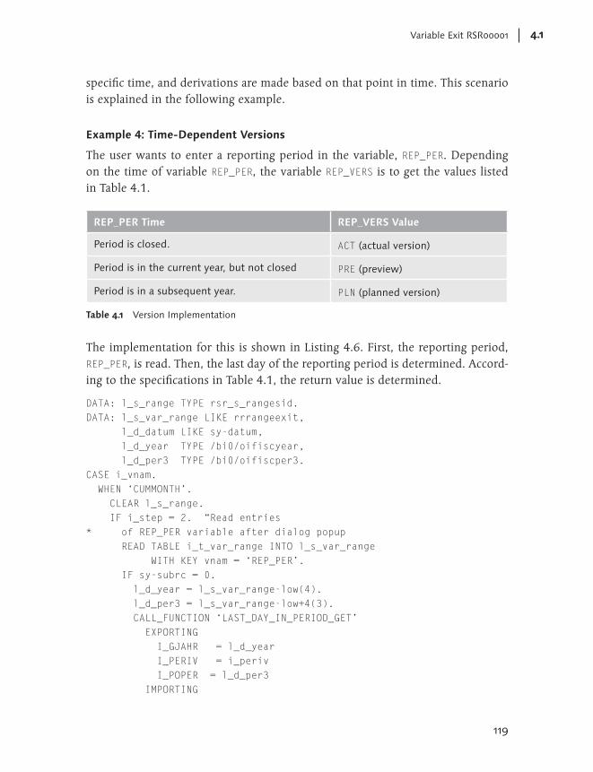
119
Variable Exit RSR00001 4.1
specific time, and derivations are made based on that point in time. This scenario is explained in the following example.
Example 4: Time-Dependent Versions
The user wants to enter a reporting period in the variable, REP_PER. Depending on the time of variable REP_PER, the variable REP_VERS is to get the values listed in Table 4.1.
REP_PER Time REP_VERS Value
Period is closed. ACT (actual version)
Period is in the current year, but not closed PRE (preview)
Period is in a subsequent year. PLN (planned version)
Table 4.1 Version Implementation
The implementation for this is shown in Listing 4.6. First, the reporting period, REP_PER, is read. Then, the last day of the reporting period is determined. Accord-ing to the specifications in Table 4.1, the return value is determined.
DATA: l_s_range TYPE rsr_s_rangesid. DATA: l_s_var_range LIKE rrrangeexit, l_d_datum LIKE sy-datum, l_d_year TYPE /bi0/oifiscyear, l_d_per3 TYPE /bi0/oifiscper3. CASE i_vnam. WHEN ‘CUMMONTH’. CLEAR l_s_range. IF i_step = 2. “Read entries * of REP_PER variable after dialog popup READ TABLE i_t_var_range INTO l_s_var_range WITH KEY vnam = ‘REP_PER’. IF sy-subrc = 0. l_d_year = l_s_var_range-low(4). l_d_per3 = l_s_var_range-low+4(3). CALL_FUNCTION ‘LAST_DAY_IN_PERIOD_GET’ EXPORTING I_GJAHR = l_d_year I_PERIV = i_periv I_POPER = l_d_per3 IMPORTING

© 2013 by Galileo Press Inc., Boston (MA)120
User Exits and BAdls in Reporting4
E_DATUM = l_d_datum EXCEPTIONS OTHERS = 1. IF SY-SUBRC <> 0. * Cannot be determined (fiscal year * variant missing?) => set default l_s_range-low = ‘ACT’. ELSE. IF l_d_datum <= sy-datum. * Period closed l_s_range-low = ‘ACT’. ELSE. CALL_FUNCTION ‘FIRST_DAY_IN_YEAR_GET’ EXPORTING I_GJAHR = l_d_year I_PERIV = i_periv IMPORTING E_DATUM = l_d_datum EXCEPTIONS OTHERS = 1. IF sy-subrc <> 0. * Cannot be determined (but could period * be determined?) => set default l_s_range-low = ‘ACT’. ELSE. IF l_d_datum > sy-datum. * Fiscal year has not yet started l_s_range-low = ‘PLN’. ELSE. l_s_range-low = ‘PRE’. ENDIF. ENDIF. ENDIF. ENDIF. ELSE. * Variable was used in error, set useful * default (e.g., ACT) l_s_range-low = ‘ACT’. ENDIF. l_s_range-sign = ‘I’. l_s_range-opt = ‘EQ’. APPEND l_s_range TO e_t_range.
Listing 4.6 Sample Variable Determination Based on Input Variables

121
Variable Exit RSR00001 4.1
Here are typical examples of variable determinations that depend on input variables.
EE Derivation of a formula variable from an input period to extrapolate annual forecasts or to distribute annual values.
EE Derivation of a comparison group (for example, a hierarchy node variable) for an input characteristic such as a profit center.
EE Derivation of upper and lower limits of a time interval that is defined not by a fixed number of periods but by other constraints, such as the beginning or end of a quarter.
EE Determination of an authorization-dependent formula variable to display periods that have not yet been released. Based on the specified period, a check is carried out as to whether the period has already been released. If not, an authorization check is performed. If the authorization check fails, 0 is returned; otherwise, 1. The query then multiplies the actual value by the result of the formula variable.
EE Derivation of variables for MultiProviders. For example, you can query a vari-able for a cost center. You then derive the profit center that’s assigned to the cost center because one of the involved InfoProviders doesn’t contain any cost center, only the profit center.
4.1.4 Implementation for I_STEP = 0
Step 0 can be used, among other things, to derive variables in authorizations. In a reporting authorization, you can simply use a variable by inserting a variable name that begins with a dollar sign ($). This variable must be defined up front in the Query Designer. When running the report, the exit is called, and you can imple-ment the authorization in ABAP.
When you determine authorizations, the return table is treated like an authorization so that all restrictions for authorizations must also be accounted for with regard to the return table. Accordingly, SIGN must always have the value I, and the value of OPT must either be EQ or BT. Excluding authorizations such as “all salaries except those of the executive board” aren’t allowed.
Possible and typical applications for these authorizations are authorization deriva-tions from tables or master data. You also can use excluding authorizations to assign an authorization dependent on the current date. Consider this typical example.

© 2013 by Galileo Press Inc., Boston (MA)122
User Exits and BAdls in Reporting4
Example 5: Changing Authorizations in the Quiet Period
In this example, we want to implement the time-dependent control of an autho-rization for a regional hierarchy. All employees have authorizations for all regions except during the so-called quiet period, which lasts from the 25th of a quarter-end month until the 15th of the following month (in January, until the 25th of January). During that time, employees are allowed to view only those regions that are stored in a table. For this purpose, their authorization contains the variable QREGION. We’ll now fill this variable in Listing 4.7. First, the current day is determined. Then, it is checked as to whether the day is in the period defined. If it is, the user can view specific regions only; otherwise, the user can view everything.
DATA: L_S_RANGE TYPE RSR_S_RANGESID. CASE i_vnam. WHEN ‘QREGION’. * Date in quiet period? DATA: l_d_tag(4) TYPE n, l_s_region TYPE z_user_region. l_d_tag = sy-datum+4(4). IF ( l_d_tag <= ‘0125’ ) OR ( ( l_d_tag >= ‘0325’ ) AND ( l_d_tag <= ‘0415’ ) ) OR ( ( l_d_tag >= ‘0625’ ) AND ( l_d_tag <= ‘0715’ ) ) OR ( ( l_d_tag >= ‘0925’ ) AND ( l_d_tag <= ‘1015’ ) ) OR ( l_d_tag >= ‘1225’ ). l_s_range-sign = ‘I’. l_s_range-opt = ‘EQ’. SELECT * FROM z_user_region INTO l_s_region WHERE uname = sy-uname. l_s_range-low = l_s_region-region. APPEND l_s_range TO e_t_range. ENDSELECT. ELSE. l_s_range-sign = ‘I’. l_s_range-opt = ‘CP’. l_s_range-low = ‘*’. APPEND l_s_range TO e_t_range. ENDIF.
Listing 4.7 Implementing an Authorization Variable
123
Variable Exit RSR00001 4.1
The IF query in Listing 4.7 normally would not be written directly in the variable but stored in a separate check function or even in a customizing table. Otherwise, those lines would have to be changed regularly in practice.
4.1.5 Implementation for I_STEP = 3
The implementation for I_STEP = 3 is different and a little more complicated than the implementation of the other steps. This is because you must make sure that not every query uses the same variables and also because not all checks are restricted to one variable.
Nevertheless, some patterns recur in variable checks. Before these patterns can be examined, you should try to minimize the problems by using a clever variable-handling strategy.
Variable Handling in SAP NetWeaver Business Warehouse
The definition of variables in SAP NetWeaver BW always causes problems because you must take into account two opposing trends. In an ideal scenario, you want to reuse the variables, but you also want to use individual texts and default values for the individual reports. Moreover, the definition of variables is very easy, so many report developers prefer to define a new variable instead of searching through the existing ones to check whether a variable exists that meets the requirements of a specific report. This attitude is perfectly understandable to those of you who have seen what happens if a variable is redefined, and then users complain about sudden occurrences of incorrect default values in live reports.
Because there’s no way to solve this problem, you should come up with a strategy that specifies how you want to use the variables. There are as many possible strategies as there are data warehouses, so the following suggestion is particularly intended for those readers who don’t yet have any strategy.
Regarding variables, there is a simple rule of thumb: You must assign an owner to each variable. This is an easy way to resolve all usage problems. The rule could be imple-mented as follows:
EE The owner of the system is responsible for all business content variables and defines central variables that can be used by everyone, such as time variables and variables for central company concepts.

© 2013 by Galileo Press Inc., Boston (MA)124
User Exits and BAdls in Reporting4
EE Each project1 is assigned a prefix and can define any variable within this namespace. Furthermore, each project can use all central variables without restriction. If a project tries to use variables from other projects, the use must be announced. In addition, the project must inform those users who have announced the use about changes to variables.
If this strategy is adhered to, various central variables will be widely used, while an even greater number of project-specific variables will be used outside of the respective projects in exceptional cases. Those who don’t comply with this strategy will probably do so when they see that one of their variables has been changed several times without prior announcement.
A consistent variable strategy has the following invaluable advantages for Step 3.
EE It’s immediately clear who is responsible for the implementation of the exit. If the validation is centrally defined, it’s centrally implemented. If not, it’s imple-mented in the project.
EE Each project knows where its variables are being used and can adjust the imple-mentation accordingly. This holds true especially for combination checks because, in those checks, it’s clear where and in which combinations the variables are used.
EE It’s clear who must be informed about changes to the exit.
If you use the example shown in Listing 4.2 for implementing the variable exit, you’ll probably ask yourself how you can implement the function module Z_VAR_CHECK_VALIDITY to meet these requirements. At this point, you can call a central function module and a function module for each project to carry out the valida-tion. This way, you can make sure that each project can validate its own variables so that identical validations don’t need to be implemented several times. On the other hand, if you do implement the identical validations, you can transport the validations separately.
In general, you must distinguish between two different cases:
EE You can validate individual variables. The variant should not be query-dependent.
EE You can validate combinations of variables. The second variant is often query-dependent because you can’t be sure that other queries don’t use the same variables.
1 By “project,” we mean an entity that defines one or several InfoProviders that are separated based on their contents, including their reports. In large BW projects, this corresponds to the sub-project level.

125
Variable Exit RSR00001 4.1
4.1.6 Validating an Individual Variable
The validation of an individual variable is relatively simple. Step 3 of the variable exit determines the variable input and checks whether the value entered by the user is permitted.
Probably the most frequent use you’ll find in practice is the validation of time entries. In this context, the check must determine whether specific intervals must have a minimum or maximum size or whether specific reports can be executed only once per quarter.
Example 6: Specifying a Quarter
A quarterly report is defined in an InfoProvider that contains the InfoObjects 0FISCPER and 0FISCPER3 as its only time characteristics. Because certain postings are made only at the end of the quarter, the report would provide incorrect results if it wasn’t run at the end of the quarter. For this reason, we define a variable, FP_QUART, which is intended to output an error if the user enters a value other than 3, 6, 9, or 12 for the period. Listing 4.8 describes the implementation.
DATA: l_s_var_range LIKE rrrangeexit. READ TABLE i_t_var_range INTO l_s_var_range WITH KEY vnam = ‘FP_QUART’. IF sy-subrc = 0. IF ( l_s_var_range-low = ‘003’ ) OR ( l_s_var_range-low = ‘006’ ) OR ( l_s_var_range-low = ‘009’ ) OR ( l_s_var_range-low = ‘012’ ). * Everything OK, don’t do anything ELSE. * The actual exception can be freely selected here. RAISE wrong_entry. ENDIF. ELSE. * If variable does not exist, do not perform any action ENDIF.
Listing 4.8 Sample Validation of a Variable
At this point, you can see that the validation you want to implement should be error-tolerant. Each line you implement here is run through for all queries irrespective of

© 2013 by Galileo Press Inc., Boston (MA)126
User Exits and BAdls in Reporting4
the variables that are actually used in the query, provided that at least one variable is used. For this reason, you shouldn’t constantly output error messages; instead you should react only if you’re sure the overall combination is wrong.
You can’t easily check whether the query contains certain characteristics. You can obtain the name of the query, but the exit doesn’t contain any definition. There-fore, it’s usually impossible to check at this point whether a variable was used for a specific characteristic or whether the characteristic exists without any constraint in the query.
4.1.7 Checking Characteristic Combinations in Step 3
The validation of multiple variables in the exit is a much more specific case. The reasons for a combination check are often as specific as the algorithms those checks are based on. Examples are characteristic values that are valid only in specific periods or variable inputs for compounded characteristics.
A frequent scenario is the validation of time intervals if they aren’t entered as inter-vals but as individual variables. This scenario is described in the following example.
Example 7: Validating Period Entries
In the following example, four variables are queried: two for “Period from and to,” and two for “Fiscal year from and to.” The exit checks whether “Fiscal year from” is smaller than “Fiscal year to” or whether “Fiscal year from” and “Fiscal year to” are equal, and whether “Period from” is smaller than or equal to “Period to.” This is implemented as shown in Listing 4.9.
DATA: l_s_var_range TYPE rrrangeexit, l_d_year_from TYPE /bi0/oifiscyear, l_d_year_to TYPE /bi0/oifiscyear, l_d_per3_from TYPE /bi0/oifiscper3, l_d_per3_to TYPE /bi0/oifiscper3. IF i_step = 3. READ TABLE i_t_var_range INTO l_s_var_range WITH KEY vnam = ‘YEARFROM’. IF sy-subrc = 0. l_d_year_from = l_s_var_range-low(4). ELSE. * If the variable does not exist, the value is set to * 0000 to make the final validation always valid.

127
Variable Exit RSR00001 4.1
l_d_year_from = ‘0000’. ENDIF. READ TABLE i_t_var_range INTO l_s_var_range WITH KEY vnam = ‘YEARTO’. IF sy-subrc = 0. l_d_year_to = l_s_var_range-low(4). ELSE. * If the variable does not exist, the value is set to * 9999 to make the final validation always valid. l_d_year_to = ‘9999’. ENDIF. READ TABLE i_t_var_range INTO l_s_var_range WITH KEY vnam = ‘PER3FROM’. IF sy-subrc = 0. l_d_per3_from = l_s_var_range-low(4). ELSE. * If the variable does not exist, the value is set to 000 * to make the final validation always valid. l_d_per3_from = ‘000’. ENDIF. READ TABLE i_t_var_range INTO l_s_var_range WITH KEY vnam = ‘PER3TO’. IF sy-subrc = 0. l_d_year_from = l_s_var_range-low(4). ELSE. * If the variable does not exist, the value is set to 999 * to make the final validation always valid. l_d_year_from = ‘999’. ENDIF. IF l_d_year_from > l_d_year_to. RAISE wrong_value. ELSEIF l_d_year_from = l_d_year_to. IF l_d_per3_from > l_d_per3_to. RAISE wrong_value. ENDIF. ENDIF. ENDIF.
Listing 4.9 Sample Validation of Characteristic Combinations
The example in Listing 4.9 shows how conscientiously you must be about ensuring that an error message is returned only if an error really occurs. Here, the validation check is carried out only if the query uses all four variables. Otherwise, setting the

© 2013 by Galileo Press Inc., Boston (MA)128
User Exits and BAdls in Reporting4
default values to 9999 for the fiscal year or 000 for the period makes sure that the lower IF queries never cause an error.
You can also see the problems involved in those queries. If only one query devel-oper uses the variables YEARFROM, PER3FROM, and PER3TO and expects the system to automatically check whether PER3FROM is smaller than or equal to PER3TO, the developer will see that this isn’t the case.
For this reason, you must either modify the query in such a way that different conditions are validated depending on the variables being used, or you must limit the query to specific queries. To do this, you must query the field, I_S_RKB1D-COMPID. The disadvantage of this variant is that new queries must be released via a corresponding specific customizing for the validation to work properly.
Returning Error Messages
The validation types described so far all work, but they have one essential drawback: The user receives only a vague error message saying that the values of the variables are invalid. However, the user doesn’t obtain any information on the variables that actually caused the error. This is why, if possible, you should store a corresponding message in the message collector in addition to the actual RAISE EXCEPTION statement.
The exit can’t return error messages by itself unlike the routines for data staging. Nor is it possible to use a MESSAGE...RAISING... call to return an adequate message because that message would simply be ignored. For this reason, you must use the same message collector used by the OLAP processor: the function module RRMS_MESSAGE_HANDLING. This function module contains the typical interface for a message collector (see Listing 4.10).
FUNCTION rrms_message_handling. *”--------------------------------------- *”*”Local interface: *” IMPORTING *” VALUE(I_CLASS) LIKE SMESG-ARBGB *” DEFAULT ‘BRAIN’ *” VALUE(I_TYPE) LIKE SMESG-MSGTY *” DEFAULT ‘S’ *” VALUE(I_NUMBER) LIKE SMESG-TXTNR *” DEFAULT ‘000’ *” VALUE(I_MSGV1) OPTIONAL *” VALUE(I_MSGV2) OPTIONAL *” VALUE(I_MSGV3) OPTIONAL *” VALUE(I_MSGV4) OPTIONAL *” VALUE(I_INTERRUPT_SEVERITY)

129
Variable Exit RSR00001 4.1
*” LIKE SY-SUBRC DEFAULT 16 *” VALUE(I_LANGU) LIKE SY-LANGU *” DEFAULT SY-LANGU *” VALUE(I_SAPGUI_FLAG) DEFAULT SPACE *” VALUE(I_SUPPRMESS) *” TYPE RSRSUPPRMESS OPTIONAL *” EXCEPTIONS *” DUMMY
Listing 4.10 Interface of Function Module RRMS_MESSAGE_HANDLING
If you want to output only plain text, you can use message 000 of message class RSBBS. However, if possible, you should create your own messages in Transaction SE91 to be able to specify a long text.
If you use this function module, the final part of the example in Listing 4.9 can then be implemented as shown in Listing 4.11.
IF l_d_year_from > l_d_year_to. CALL FUNCTION ‘RRMS_MESSAGE_HANDLING’ EXPORTING I_CLASS = ‘RSBBS’ I_TYPE = ‘I’ I_NUMBER = ‘000’ I_MSGV1 = ‘Year from bigger than year to’. RAISE WRONG_VALUE. ELSEIF l_d_year_from = l_d_year_to. IF l_d_per3_from > l_d_per3_to. CALL FUNCTION ‘RRMS_MESSAGE_HANDLING’ EXPORTING I_CLASS = ‘RSBBS’ I_TYPE = ‘I’ I_NUMBER = ‘000’ I_MSGV1 = ‘Month from bigger than month to’. RAISE WRONG_VALUE. ENDIF. ENDIF.
Listing 4.11 Example of Using Messages
Of course, you can also use the function module RRMS_MESSAGE_HANDLING to return error messages in the other steps of the exit, which always makes sense.

© 2013 by Galileo Press Inc., Boston (MA)130
User Exits and BAdls in Reporting4
4.2 Virtual Key Figures and Characteristics
Another exit frequently used in SAP NetWeaver BW is the exit for virtual key figures and characteristics. Virtual key figures and characteristics are InfoObjects that are contained in the InfoProvider, but whose values aren’t read from the InfoProvider. Instead, the values are determined at the time the query is run. There are many reasons for this; these are the most frequent:
EE You want to carry out calculations that are too complex for query formulas and for which you don’t have all necessary information at the time of loading.
EE You want to integrate data from several InfoProviders, but the results provided by the MultiProvider are insufficient.
EE You must carry out calculations at a level that is more detailed than the query. This happens, for example, if costs are calculated as a product of quantity and price at purchase-order level, while the query presents the results at sales depart-ment level.
EE You want to carry out complex calculations based on user input.
EE You want to display specific values based on the time the query is executed or hide those values (during the quiet period, see Example 5 in Section 4.1.4).
In all these cases, you’ll have to use virtual key figures and characteristics.
The advantage of virtual key figures and characteristics is that they make report-ing much more flexible. The ability to generate values at the time a query is run provides simple solutions to various problems that otherwise would have to be calculated manually.
However, this method also has one drawback: Each calculation that’s carried out at this point affects the performance during the query execution. Therefore, you must consider two factors. First, you should try to avoid any kind of database access. Second, the exit enables you to read additional characteristics from the database. This means that existing queries no longer access existing aggregates.
This can have a substantial impact, particularly because the exit is called once per data record, and the data record in turn is read from the database. If the records are read from an aggregate, the number of records read from the database is sig-nificantly smaller. For this reason, it’s important to always test the exit by using (almost) live data, particularly with regard to the number of data records, when you use virtual key figures and characteristics.

131
Virtual Key Figures and Characteristics 4.2
Testing the Use of Virtual Key Figures
In a customer system, the exit for virtual key figures was run in a test system with approximately 500 data records without any error and then transported into the live system. When the respective report was called in the live system, it took two hours before the report returned the required data. In this case, the data was wrong because not all combinations had been tested in the test system.
4.2.1 Implementation
Those of you who have experience with virtual key figures and characteristics may remember the user exit RSR00002, which allowed you to implement virtual Info Objects before BW release 3.0. This user exit was very difficult to implement because it required the creation of specific form routines with fixed naming con-ventions in certain includes. Consequently, it was as easy to make mistakes as it was difficult to find those mistakes.
This is why we want to focus on describing how to implement virtual key figures and characteristics using the BAdI RSR_OLAP_BADI. Compared to the old implemen-tation, this BAdI has the following three advantages:
EE You can create different implementations that can even be restricted to different InfoProviders.
EE You need to implement only two methods. A relatively simple pattern is avail-able for both of these. This pattern facilitates the implementation. A third method that is available in the BAdI can be copied unmodified from the sample imple-mentation.
EE There are no large confusing includes.
These three factors make it easier to implement virtual key figures and characteris-tics in such a way that after you have implemented the BAdI once or twice, you’ll be able to quickly create more.
The following describes an example in which you would want to implement the display of customer contacts. An InfoProvider contains purchase orders that include customer numbers and sales offices. A DataStore object, CCONTACT (current contact), contains one contact (CONTACT) per sales office (SALESOFF) and customer number (0CUSTOMER). The sales office and customer number aren’t compounded. You want to create a report that displays the current contact depending on the sales office.

© 2013 by Galileo Press Inc., Boston (MA)132
User Exits and BAdls in Reporting4
To do this, the DataStore must be read at report runtime because it’s impossible to reload the complete purchase order InfoProvider if the contacts change.
Step 1: Creating the BAdI Implementation
1. Call Transaction SE19 to create a BAdI implementation. This transaction was completely revised for SAP NetWeaver 7.0.
2. In SAP NetWeaver 7.x, go to the Create Implementation section, and choose the Classic BAdI radio button (see Figure 4.1).
Figure 4.1 Creating a BAdI in SAP NetWeaver 7.x
3. Enter the name of the BAdI definition. For virtual key figures and characteristics, that’s “RSR_OLAP_BADI”. Click on the Create Impl. button.
4. Enter a corresponding name in the dialog box that follows, for example, “ZAN-PART” (see Figure 4.2).

133
Virtual Key Figures and Characteristics 4.2
Figure 4.2 Dialog Box for Querying the Implementation
5. The dialog box that follows prompts you for the BAdI definition. The BAdI definition for virtual key figures and characteristics is called “RSR_OLAP_BADI”.
6. After you have confirmed your entry by pressing (Enter), the attributes of the BAdI implementation are displayed. Assign an Implementation Short Text, and, in the lower part of the screen, select the InfoProvider for which you want to create the implementation. Masked entries are also allowed. In our example, the InfoProvider is called ORDERS (see Figure 4.3).
Figure 4.3 Properties of the BAdI

© 2013 by Galileo Press Inc., Boston (MA)134
User Exits and BAdls in Reporting4
7. Save the BAdI implementation prior to copying the sample code provided by SAP via Goto • Sample Coding • Copy. This step is important because the sample code contains the complete INITIALIZATION method, which means you don’t need to change that.
8. Go to the Interface tab (see Figure 4.4). You’ll see that the BAdI contains three methods for implementation: DEFINE, INITIALIZATION, and COMPUTE. You need to implement only the first and the last one.
Moreover, at this point, you can still change the name of the class to be imple-mented. But you should do that only in exceptional cases. The class name sug-gested by the system can be clearly derived from the name of the implementation so that the class name clearly indicates that the implementation is a BAdI implementation.
Figure 4.4 Interface of the BAdI
Step 2: Implementing the DEFINE Method
In the next step, you implement the DEFINE method. The DEFINE method is called at the time the query is generated, and it tells the system which characteristics

135
Virtual Key Figures and Characteristics 4.2
and key figures are virtual and which ones are required for calculating the virtual characteristics.
The method contains the interface shown in Table 4.2.
Type Parameter Type Description
I FLT_VAL RSR_OLAP_BADI_FLT
FLT_VAL specifies the filter that is defined in the interface.
I I_S_RKB1D RSR_S_RKB1D
I_S_RKB1D is the same parameter that is used in the interface for user exit EXIT_SAPLRRS0_001. It contains information on the query being used, particularly on the InfoProvider that is used.
I I_TH_CHANM_USED
RRKE_TH_CHANM
I_TH_CHANM_USED contains all characteris-tics used in the query. Characteristics that don’t exist in the query don’t need to be calculated.
I I_TH_KYFNM_USED
RRKE_TH_KYFNM
I_TH_KYFNM_USED contains all key figures used in the query. This is important to ensuring that key figures that don’t exist in the query don’t need to be calculated.
C C_T_CHANM RRKE_T_CHANM
C_T_CHANM and C_T_KYFNM must be filled in the method. That’s where the characteristics and key figures that are to be filled and are required as a precondition are included. In addition to the InfoObject, C_T_CHANM contains the read mode in the MODE field. This field has two values: RRKE_C_MODE-READ makes sure that the InfoObject is read from the database, while RRKE_C_MODE-NO_SELECTION makes sure that the InfoObject isn’t read from the database and that it can be filled in the COMPUTE method instead.
C C_T_KYFNM RSD_T_KYFNM
X CX_RS_ERROR
In case of a severe error, the exception CX_RS_ERROR can be triggered.
I = Importing, E = Exporting, C = Changing, X = Exception
Table 4.2 Signature of the DEFINE Method

© 2013 by Galileo Press Inc., Boston (MA)136
User Exits and BAdls in Reporting4
1. Double-click on the method name DEFINE to go to the ABAP Editor where you want to implement the method. For this example, you should enter the code shown in Listing 4.12.
METHOD IF_EX_RSR_OLAP_BADI~DEFINE . DATA: l_s_chanm TYPE rrke_s_chanm, l_s_chanm_used TYPE rschanm, l_kyfnm TYPE rsd_kyfnm. CASE i_s_rkb1d-infocube. WHEN ‘ORDER’. LOOP AT i_th_chanm_used INTO l_s_chanm_used. CASE l_s_chanm_used. * Here the required InfoObjects are queried WHEN ‘CONTACT’. l_s_chanm-chanm = ‘CONTACT’. l_s_chanm-mode = rrke_c_mode-no_selection. APPEND l_s_chanm TO c_t_chanm. l_s_chanm-chanm = ‘SALESOFF’. l_s_chanm-mode = rrke_c_mode-read. APPEND l_s_chanm TO c_t_chanm. l_s_chanm-chanm = ‘0CUSTOMER’. l_s_chanm-mode = rrke_c_mode-read. APPEND l_s_chanm TO c_t_chanm. ENDCASE. ENDLOOP. * LOOP AT i_t_kyfnm_used into l_kyfnm. * CASE l_kyfnm. * WHEN ‘...’. * APPEND l_kyfnm TO c_t_kyfnm. * ENDCASE. * ENDLOOP. ENDCASE.
Listing 4.12 Implementing the DEFINE Method
It usually makes sense to have the DEFINE method begin with a CASE query on InfoProvider I_S_RKB1D-INFOCUBE, even though you can use only one Info-Provider. If you do that, you can already see in the code that InfoProvider the definition runs on.
2. The required characteristics must be inserted in table C_T_CHANM. A decisive fac-tor regarding functionality is the read mode, L_S_CHANM-MODE.

137
Virtual Key Figures and Characteristics 4.2
Two read modes are available:
EE RRKE_C_MODE-READ reads the characteristic from the database in any case, even if it isn’t used in the query. For this reason, you may no longer be able to use existing aggregates.
EE RRKE_C_MODE-NO_SELECTION doesn’t read the characteristic from the database. Instead, it marks the characteristic as virtual. This means it can be modified in the BAdI.
3. If the contact is contained in the query, the sales office and the customer num-ber must also be read so that the contact can be derived. So the query uses only aggregates that contain SALESOFF and 0CUSTOMER. After that, the key figures fol-low. The key figures don’t require a read mode.
4. Finally, you must save and activate the method.
Object-Oriented Programming
At this point, it’s inevitable that you will take a quick look at object-oriented program-ming because you will have to create attributes for a class. But we’ll focus on the required technique without going into the theoretical details. You should regard the instance attributes as a kind of global variable.
Step 3: Creating the Instance Attributes
1. If you double-click on the INITIALIZATION method to take a look at it, you see a complete implementation that doesn’t need to be changed. This method is used to facilitate the implementation of the COMPUTE method. However, you must first do some preparatory work.
2. Double-click on the name of the implementing class in the Interface tab of the BAdI to go to the class definition (see Figure 4.4). Then select the Attributes tab (see Figure 4.5).
3. Now you must include an attribute for each InfoObject that you inserted into the C_T_CHANM and C_T_KFNM tables in the DEFINE method. For characteristics, this attribute is called P_CHA_<InfoObject>; for key figures, P_KYF_<InfoObject>. All attributes are instance attributes that have the visibility Public of type I.
For this case, you must create three public instance attributes: P_CHA_CONTACT, P_CHA_0CUSTOMER, and P_CHA_SALESOFF. These attributes are necessary because the structure that is transferred to the COMPUTE method doesn’t contain any

© 2013 by Galileo Press Inc., Boston (MA)138
User Exits and BAdls in Reporting4
typical field names such as /BIC/CONTACT. Instead, it contains field names such as K_022.
To access the correct fields, the INITIALIZATION method fills the attributes as follows. If the InfoObject is contained in the query, the attribute P_CHA_<InfoObject> is assigned a value greater than 0. This value indicates the position of the InfoObject within the structure. If the query doesn’t contain the InfoObject, the value is 0. These attributes are used in the COMPUTE method to access the appropriate field via an ASSIGN COMPONENT.
4. In addition, you need another attribute that buffers the data of the DataStore object. For this purpose, you need a Z_TH_CCONTACT table type that references a hashed table with the structure /BIC/ACCONTACT00.
5. Create a static attribute, _TH_CCONTACT, that has the corresponding table type. The result is displayed in Figure 4.5.
Figure 4.5 Attributes of the ZCL_IM_CONTACT Class
Step 4: Implementing the COMPUTE Method
Now you can implement the COMPUTE method:
1. Double-click on the method name COMPUTE in the Interface tab of the BAdI implementation to go to the implementation of the method that contains the interface from Table 4.3.

139
Virtual Key Figures and Characteristics 4.2
Type Parameter Type Description
I FLT_VAL RSR_OLAP_BADI_FILTER
FLT_VAL specifies the filter that is stored in the BAdI.
I I_PARTCUBE RSD_INFOCUBE I_PARTCUBE specifies the subprovider of the MultiProvider from which the current data record originates.
I I_S_RKB1D RSR_S_RKB1D I_S_RKB1D is the same parameter that is used in the interface for user exit EXIT_SAPLRRS0_001. It contains information on the query being used, particularly on the InfoProvider that is used.
I I_NCUM RS_BOOL I_NCUM specifies whether the InfoProvider contains inventory values.
C C_S_DATA ANY C_S_DATA is the structure that contains the values from the database in the structure that’s necessary for the query. This structure also contains the fields that were included in the C_T_CHANM and C_T_KYFNM tables in the DEFINE method. However, the field names don’t correspond to the usual field names in database tables.
I = Importing, C = Changing
Table 4.3 Signature of the COMPUTE Method
2. In this method, you will implement the actual calculation of the virtual character-istics. The implementation of the method consists of two parts. The first part is standardized and is used to assign input and output values to field symbols. The second part contains the actual calculation. The first part is shown in Listing 4.13.
METHOD IF_EX_RSR_OLAP_BADI~COMPUTE . FIELD-SYMBOLS: <l_contact> TYPE /bic/oicontact, <l_customer> TYPE /bi0/oicustomer, <l_salesoff> TYPE /bic/oisalesoff. * Assign field symbols using instance attributes IF p_cha_contact > 0. ASSIGN COMPONENT p_cha_contact

© 2013 by Galileo Press Inc., Boston (MA)140
User Exits and BAdls in Reporting4
OF STRUCTURE c_s_data TO <l_contact>. ELSE. * If virtual characteristic does not exist, exit routine EXIT. ENDIF. IF p_cha_customer > 0. ASSIGN COMPONENT p_cha_customer OF STRUCTURE c_s_data TO <l_customer>. ELSE. * If source characteristic does not exist, initialize * CONTACT and exit routine CLEAR <l_contact>. EXIT. ENDIF. IF p_cha_salesoff > 0. ASSIGN COMPONENT p_cha_salesoff OF STRUCTURE c_s_data TO <l_salesoff>. ELSE. * If source characteristic does not exist, initialize * CONTACT and exit routine CLEAR <l_contact>. EXIT. ENDIF.
Listing 4.13 First Part of the Implementation of the COMPUTE Method
The decisive command is always ASSIGN COMPONENT p_.... This command must be entered for each InfoObject that is required for the calculation. Because the exit is usually executed for each query on the InfoProvider, you must always be able to react to the fact that certain InfoObjects aren’t contained in the query; sometimes you may even skip the entire calculation.
3. After all field symbols have been assigned in this way, the actual calculation can begin (see Listing 4.14).
IF _th_contact[] IS INITIAL. SELECT * FROM /bic/accontact00 INTO TABLE _th_ccontact. ENDIF. DATA: l_s_ccontact TYPE /bic/acontact00. READ TABLE _th_ccontact INTO l_s_ccontact
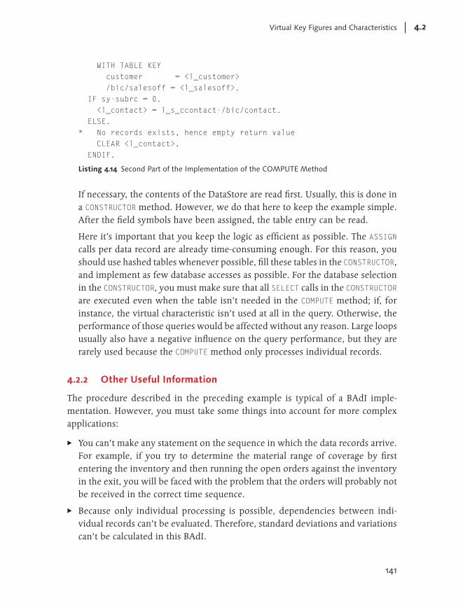
141
Virtual Key Figures and Characteristics 4.2
WITH TABLE KEY customer = <l_customer> /bic/salesoff = <l_salesoff>. IF sy-subrc = 0. <l_contact> = l_s_ccontact-/bic/contact. ELSE. * No records exists, hence empty return value CLEAR <l_contact>. ENDIF.
Listing 4.14 Second Part of the Implementation of the COMPUTE Method
If necessary, the contents of the DataStore are read first. Usually, this is done in a CONSTRUCTOR method. However, we do that here to keep the example simple. After the field symbols have been assigned, the table entry can be read.
Here it’s important that you keep the logic as efficient as possible. The ASSIGN calls per data record are already time-consuming enough. For this reason, you should use hashed tables whenever possible, fill these tables in the CONSTRUCTOR, and implement as few database accesses as possible. For the database selection in the CONSTRUCTOR, you must make sure that all SELECT calls in the CONSTRUCTOR are executed even when the table isn’t needed in the COMPUTE method; if, for instance, the virtual characteristic isn’t used at all in the query. Otherwise, the performance of those queries would be affected without any reason. Large loops usually also have a negative influence on the query performance, but they are rarely used because the COMPUTE method only processes individual records.
4.2.2 Other Useful Information
The procedure described in the preceding example is typical of a BAdI imple-mentation. However, you must take some things into account for more complex applications:
EE You can’t make any statement on the sequence in which the data records arrive. For example, if you try to determine the material range of coverage by first entering the inventory and then running the open orders against the inventory in the exit, you will be faced with the problem that the orders will probably not be received in the correct time sequence.
EE Because only individual processing is possible, dependencies between indi-vidual records can’t be evaluated. Therefore, standard deviations and variations can’t be calculated in this BAdI.

© 2013 by Galileo Press Inc., Boston (MA)142
User Exits and BAdls in Reporting4
EE Moreover, you can’t create or insert any additional records in this BAdI. If not all characteristic combinations are available in the InfoProvider, you can’t gene-rate any additional ones.
EE In individual cases, the relationship between virtual characteristics and the elimination of intercompany sales can be important. The elimination of inter-company sales doesn’t consider the virtual characteristics; the elimination is based on the values that are originally stored in the InfoCube. This fact prevents you from creating some nice solutions that would use the elimination of inter-company sales to adjust the hierarchy aggregation.
4.2.3 Transferring Variable Values to the BAdI
Another option to make the BAdI more flexible is the transfer of variables. For this purpose, a static public attribute is created in the implementing class for each variable to be transferred to the BAdI.
The actual transfer of the variable occurs in Step 3 of exit EXIT_SAPLRRS0_001. You can use the code shown in Listing 4.15, and in the BAdI, you can simply access the value ZCL_IM_CONTACT=>MY_VAR. If you want to transfer intervals and selection options, the query must be modified accordingly.
DATA: l_s_var_range LIKE rrrangeexit. READ TABLE i_t_var_range INTO l_s_var_range WITH KEY vnam = ‘MY_VAR’. IF SY-SUBRC = 0. zcl_im_anpart=>my_var = l_s_var_range-low. ENDIF.
Listing 4.15 Sample Variable Transfer to a BAdI
Variables can be particularly useful in restricting a possible selection right from the start. Instead of reading the entire contents of a DataStore object, only the required records are read. It can also be useful to transfer formula variables or posting periods to the exit if you want to implement specific nonlinear extrapolations.
The virtual key figures and characteristics represent a very efficient way to extend the reporting functionality. Because you can access variables and also add more database tables to the calculation, you can bypass many restrictions of SAP NetWeaver BW.
143
VirtualProvider 4.3
However, because the BAdI is called at a sensitive point, namely after the data has been read from the database, the implementation must be very clean to avoid problems in reporting performance.
Furthermore, you must always take into account that the BAdI is called for all que-ries that run on the corresponding InfoProviders even if the virtual characteristics and key figures aren’t used. Here you must ensure that calculations and especially database selections are carried out only if they are really required.
4.3 VirtualProvider
If you think that the exits discussed so far aren’t flexible enough to provide the required results, your last resort is the VirtualProvider, or rather the VirtualProvider that’s based on a function module (in SAP BW 3.x it was called RemoteCube with services). By definition, a VirtualProvider is an InfoProvider that doesn’t store the data by itself but reads the data from other data sources that aren’t InfoProviders (as opposed to MultiProviders). In this context, three DataSources are relevant:
EE The data is read from a DataSource (for example, directly from the source system)
EE The data is read from a table using a BAPI
EE The data is calculated using a function module
The third method, in particular, provides a lot of options for designing a report, but its implementation is complex and exceeds the scope of this book. The following sections describe how you can create a VirtualProvider and which interfaces you must implement; however, we don’t provide any extensive sample implementations.
Avoiding Rounding Differences
If, in an annual report, certain overview reports are presented in terms of thousands, rounding differences are very likely to occur (for example, $500,000 + $500,000 = $1,000,000 would be represented as 1+1=1 in terms of thousands). If you try to round off the results during the loading process, the totals will no longer match. For this reason, you could use a VirtualProvider to read the basic data and convert it to thousands, then aggregate both values on the basis of the transferred variables, calculate the difference, and distribute the difference downward. Some developers prefer to correct the round-ing differences manually.
Interestingly, it’s much easier to include an additional line for the rounding difference in the program code and show the rounding difference there.

© 2013 by Galileo Press Inc., Boston (MA)144
User Exits and BAdls in Reporting4
4.3.1 Creating a VirtualProvider
You can create a VirtualProvider via the context menu of an InfoProvider. You have three options for a VirtualProvider (see Figure 4.6).
Figure 4.6 Creating a VirtualProvider
From the point of view of an ABAP developer, the most interesting and most flexible VirtualProvider is the VirtualProvider <Euro2>N Based on Function Module path. If you select this VirtualProvider and click on the Details button, various control checkboxes are displayed. For the implementation, the checkboxes RFC Packing and SID Support are of particular importance because the interface

145
VirtualProvider 4.3
of the function module to be implemented changes depending on these switches. The following scenarios are possible.
Case 1: RFC Packing Is Set
If RFC Packing is set for the VirtualProvider, the interface is structured as shown in Listing 4.16.
IMPORTING infocube LIKE bapi6200-infocube keydate LIKE bapi6200-keydate EXPORTING return LIKE bapiret2 TABLES selection STRUCTURE bapi6200sl characteristics STRUCTURE bapi6200fd keyfigures STRUCTURE bapi6200fd data STRUCTURE bapi6100da EXCEPTIONS communication_failure system_failure
Listing 4.16 Interface of the VirtualProvider (RFC Packing)
This is the standard case, which should be used whenever possible. The interface is implemented in function module BAPI_INFOCUBE_READ_REMOTE_DATA, which you can use as a template module. It also contains a comprehensive documentation.
Because the parameters can’t be derived from the interface without difficulty, we briefly describe them here.
EE INFOCUBE is the name of the VirtualProvider.
EE KEYDATE is the key date on which the query is run and on which the master data should be read. However, you’ll see further on that you have to read the naviga-tion attributes by yourself. In doing so, you don’t have to adhere to the key date, but you should do so to avoid confusing the reader. You can implement different key dates for different navigation attributes.
EE RETURN is the standard return structure of each BAPI. BAPIs are Business Appli-cation Interfaces and contain the SAP Business Logic encapsulated in function modules. You should make sure that the function module to be implemented should behave like a BAPI. In particular, it should not end with an X message,

© 2013 by Galileo Press Inc., Boston (MA)146
User Exits and BAdls in Reporting4
which causes the program to abort. Instead, the function module should always provide a clean return and, if necessary, an abort message. Otherwise, the user will have to wait in front of the Business Explorer (BEx) screen because the sys-tem isn’t able to detect that the data-retrieval process in SAP NetWeaver BW has terminated.
EE SELECTION contains the selections that are defined in the query. Variables have already been replaced with input or replacements. The structure of the table is EXPRESSION, INFOOBJECT, SIGN, OPTION, LOW, HIGH.
The most important field here is the EXPRESSION field: If the value of this field is 0, the corresponding restriction is a global filter. If the value isn’t 0, the restric-tion refers to a row, column, or cell reference. This is of decisive importance for data selections that must be implemented. It makes a big difference whether in a query a column is restricted to the country “USA” and the sales channel “Inter-net,” or a query contains two columns and one of them is restricted to the coun-try “USA” while the other is restricted to the sales channel “Internet.”
If several values exist for EXPRESSION, the logic to be implemented requires that all those records from the database are read to which the restriction E0 and at least one of the restrictions E1 through En apply. The documentation for func-tion module BAPI_INFOCUBE_READ_REMOTE_DATA describes this logic in the fol-lowing way:
E0 AND ( E1 OR E2 OR E3 ... OR En )
A better way of presenting this logic is to display it as follows:
( E0 AND E1 ) OR ( E0 AND E2 ) OR ( E0 AND E3 ) ... OR ( E0 AND En ).
This way, you can regard each statement as a separate line or column of a query.
EE CHARACTERISTICS and KEYFIGURES are two tables that contain the characteristics and key figures used in the query. Both tables have the same structure: INFO-OBJECT, DATATYPE, DECIMALS, SIGN, LENGTH, OFFSET, LOWERCASE. The LENGTH and OFFSET fields are particularly important here. These fields indicate in which position and at what length the InfoObject can be found in the return structure.
As already mentioned, not only are the characteristics transferred in the CHARAC-TERISTICS table but also the navigation attributes used in the query.

147
VirtualProvider 4.3
EE DATA is the table that contains the return values for the OLAP processor. This table consists of only the CONTINUATION and DATA fields. Because it’s a BAPI, the length of the DATA field can’t be variable; it always consists of 250 characters.
If the return structure contains more than 250 characters, it must be distributed to several rows in the DATA table. To do this, you can use the CONTINUATION field. Each line of a data record except for the last one is assigned the value X in this field. The field remains empty in the last record. Therefore, it must be interpreted as “Data record will continue in the next row.”
The class CL_RSDRV_REMOTE_IPROV_SRV contains some useful methods and services for implementing this BAPI. This class is predominantly used to implement the BAPI for reading data from a database table.
Case 2: RFC Packing and SID Support Are Not Set
If neither RFC Packing nor SID Support is set, the interface is structured as shown in Listing 4.17.
IMPORTING i_infoprov TYPE rsinfoprov i_keydate TYPE rrsrdate i_th_sfc TYPE rsdri_th_sfc i_th_sfk TYPE rsdri_th_sfk i_t_range TYPE rsdri_t_range i_tx_rangetab TYPE rsdri_tx_rangetab i_first_call TYPE rs_bool i_packagesize TYPE i EXPORTING e_t_data TYPE standard table e_end_of_data TYPE rs_bool e_t_msg TYPE rs_t_msg
Listing 4.17 Interface of the VirtualProvider (Neither RFC Packing nor SID Support Are Set)
Instead of the BAPI structures, this interface contains the structures that are used internally by SAP NetWeaver BW. Whereas in Case 1, the function module is called only once, the generated function module is called several times in this imple-mentation; that is, it’s called until the E_END_OF_DATA parameter is set to RS_TRUE. For each call, I_PACKAGESIZE records are expected. However, this default setting comes from system customizing and can be ignored. If so many data records must be returned that the DATA table described in Listing 4.16 would significantly affect

© 2013 by Galileo Press Inc., Boston (MA)148
User Exits and BAdls in Reporting4
system performance or cause the main memory to overflow, you should consider implementing the variant described in Listing 4.17.
Case 3: RFC Packing Is Not Set; SID Support Is Set
In all other cases, that is, if RFC Packing isn’t set and SID Support is set, the vari-ant is referred to as “internal,” and it indicates that the interface can be modified without a warning. For this reason, you should use Case 1. For the intrepid among you, however, Listing 4.18 contains the interface for Case 3.
IMPORTING i_infoprov TYPE rsinfoprov i_keydate TYPE rrsrdate i_th_sfc TYPE rsdd_th_sfc i_th_sfk TYPE rsdd_th_sfk i_tsx_seldr TYPE rsdd_tsx_seldr i_first_call TYPE rs_bool i_packagesize TYPE i EXPORTING e_t_data TYPE standard table e_end_of_data TYPE rs_bool e_t_msg TYPE rs_t_msg
Listing 4.18 Interface of the VirtualProvider (RFC Packing Is Not Set, SID Support Is Set)
When implementing this, you should note that SID Support doesn’t mean that you will be supported in defining the SIDs. It means that in addition to the char-acteristic values, you must also return the SIDs for the data records. This variant is used by the SAP development team, for instance, to implement additional logic in SAP SEM-BCS. For each InfoProvider that stores data, SAP SEM-BCS creates a VirtualProvider in which reporting takes place. This VirtualProvider also uses a cor-responding service that reads the InfoProvider and the SIDs at the same time. This means the OLAP processor doesn’t need to further determine the SIDs afterward.
4.3.2 Do’s and Don’ts for the Implementation of the Service
Similar to the implementation of virtual key figures and characteristics, the imple-mentation of a VirtualProvider is critical because it’s called for each query. For this reason, you should absolutely adhere to the following restrictions:
149
VirtualProvider 4.3
EE If your DataSource isn’t a small table containing some 1,000 data records, you should read only what has been transferred in the query.
EE You should read only the requested characteristic values and, if possible, have those records aggregated by the database.
EE Similarly, you should read only the required key figures from the database. Especially when the query is run, every additional byte is inconvenient, par-ticularly if the query is used by many users. Nothing is more annoying in the BW system than having users wait too long for a query to be run. This immedi-ately decreases the degree of acceptance of the system as a whole.
It’s relatively easy to read data from master data tables and DataStore objects because this data is stored in flat tables, and every developer can implement the SELECT statements by himself, regardless of optimization aspects. But what can you do if the data is stored not in a DataStore object but in an InfoCube? You have two options: loading the data into a DataStore object or into a standard SAP function module.
If you don’t need the entire InfoCube but only aggregated data that refers to a relatively small number of data records (in SAP NetWeaver BW, this means approxi-mately 100,000 records, depending on the design of the system and the structure of the data), you can create a DataStore object with the required structure, load the data into the DataStore via an export DataSource, and obtain the required aggrega-tion. To do this, however, you need additional hard disk space. But why should you store the data once again when it’s already stored in a form that’s optimized for database access, namely the star schema of the InfoCube? That’s why you must find an efficient way to access the contents of the InfoCube.
One option is to use function module RSDRI_INFOPROV_READ. Although this func-tion module has not been officially released by SAP, it has been used successfully in the past, even for larger quantities of data. This function module has several advantages. You can assign the required characteristics and key figures to it, and the function module automatically carries out a data aggregation. Further, it uses the parameters assigned to it to automatically select an aggregate, which it then uses for data selection. It’s this feature, in particular, that enables you to build VirtualProviders that access InfoProviders containing millions of data records and still return a query result within a couple of seconds.
The interface of the function module is described in Listing 4.19.

© 2013 by Galileo Press Inc., Boston (MA)150
User Exits and BAdls in Reporting4
FUNCTION rsdri_infoprov_read . *”--------------------------------------- *”*”Local interface: *” IMPORTING *” REFERENCE(I_INFOPROV) *” TYPE RSINFOPROV *” REFERENCE(I_TH_SFC) *” TYPE RSDRI_TH_SFC *” REFERENCE(I_TH_SFK) *” TYPE RSDRI_TH_SFK *” REFERENCE(I_T_RANGE) *” TYPE RSDRI_T_RANGE OPTIONAL *” REFERENCE(I_TH_TABLESEL) *” TYPE RSDRI_TH_SELT OPTIONAL *” REFERENCE(I_T_RTIME) *” TYPE RSDRI_T_RTIME OPTIONAL *” VALUE(I_REFERENCE_DATE) *” TYPE RSDRI_REFDATE *” DEFAULT SY-DATUM *” VALUE(I_ROLLUP_ONLY) *” TYPE RS_BOOL DEFAULT RS_C_TRUE *” REFERENCE(I_T_REQUID) *” TYPE RSDR0_T_REQUID OPTIONAL *” VALUE(I_SAVE_IN_TABLE) *” TYPE RSDRI_SAVE_IN_TABLE *” DEFAULT SPACE *” VALUE(I_TABLENAME) *” TYPE RSDRI_TABLENAME OPTIONAL *” VALUE(I_SAVE_IN_FILE) *” TYPE RSDRI_SAVE_IN_FILE *” DEFAULT SPACE *” VALUE(I_FILENAME) *” TYPE RSDRI_FILENAME OPTIONAL *” VALUE(I_PACKAGESIZE) *” TYPE I DEFAULT 1000 *” VALUE(I_MAXROWS) TYPE I DEFAULT 0 *” VALUE(I_AUTHORITY_CHECK) *” TYPE RSDRI_AUTHCHK DEFAULT *” DEFAULT RSDRC_C_AUTHCHK-READ *” VALUE(I_CURRENCY_CONVERSION) *” TYPE RSDR0_CURR_CONV *” DEFAULT ‘X’ *” VALUE(I_USE_DB_AGGREGATION)

151
VirtualProvider 4.3
*” TYPE RS_BOOL *” DEFAULT RS_C_TRUE *” VALUE(I_USE_AGGREGATES) *” TYPE RS_BOOL *” DEFAULT RS_C_TRUE *” VALUE(I_READ_ODS_DELTA) *” TYPE RSDRI_CHANGELOG_EXTRACTION *” DEFAULT RS_C_FALSE *” VALUE(I_CALLER) *” TYPE RSDRS_CALLER *” DEFAULT RSDRS_C_CALLER-RSDRI *” VALUE(I_DEBUG) *” TYPE RS_BOOL *” DEFAULT RS_C_FALSE *” VALUE(I_CLEAR) *” TYPE RS_BOOL *” DEFAULT RS_C_FALSE *” EXPORTING *” REFERENCE(E_T_DATA) *” TYPE STANDARD TABLE *” VALUE(E_END_OF_DATA) *” TYPE RS_BOOL *” VALUE(E_AGGREGATE) *” TYPE RSINFOCUBE *” VALUE(E_SPLIT_OCCURRED) *” TYPE RSDR0_SPLIT_OCCURRED *” REFERENCE(E_T_MSG) TYPE RS_T_MSG *” CHANGING *” REFERENCE(C_FIRST_CALL) *” TYPE RS_BOOL *” EXCEPTIONS *” ILLEGAL_INPUT *” ILLEGAL_INPUT_SFC *” ILLEGAL_INPUT_SFK *” ILLEGAL_INPUT_RANGE *” ILLEGAL_INPUT_TABLESEL *” NO_AUTHORIZATION *” ILLEGAL_DOWNLOAD *” ILLEGAL_TABLENAME *” TRANS_NO_WRITE_MODE *” INHERITED_ERROR *” X_MESSAGE
Listing 4.19 Interface of Function Module RSDRI_INFOPROV_READ

© 2013 by Galileo Press Inc., Boston (MA)152
User Exits and BAdls in Reporting4
At first glance, this table appears shocking. What is important in this function module is the IMPORTING parameter I_INFOPROV that contains the name of the InfoProvider plus I_TH_SFC and I_TH_SFK. These two tables contain the characteristics (I_TH_SFC) and key figures (I_TH_SFK) that are to be read from the InfoProvider. Most of the other parameters are self-explanatory and can be ignored. It’s also advisable to set a breakpoint in the function module and to call Transaction LISTCUBE. Overall, the function module is very powerful; try it for yourself.
If you want to use the function module in the VirtualProvider, you will certainly receive an error message telling you that the function module must not be called recursively. The reason for this is that the same function module is used to read data from the VirtualProvider. In that case, you should create an RFC-enabled function module that wraps the part of the interface you need. Then you can call the newly created function module via RFC.
Nevertheless, it’s clearly preferable that your users are flexible enough to avoid using VirtualProviders with services. Usually these InfoProviders require more maintenance work, and it’s more time-consuming to extend queries than to use normal InfoCubes or MultiProviders. If possible, you should always try to convince your customer of a solution that meets his requirements by using virtual key figures and characteristics. Always remember that it’s possible to carry out some of the calculations in a Microsoft Excel worksheet.
4.4 BAdI SMOD_RSR00004
Finally, let’s look at BAdI SMOD_RSR00004, which originated from user exit RSR00004 and was automatically migrated from it. This BAdI is called in the report-report interface, where it’s used to carry out automatic adjustments. You can use this function, for example, to modify an InfoObject.
For instance, if you display those cost centers in a report that services a specific purchase order, and if you want to display a cost report for the cost center, the cost center will be contained in InfoObject 0PCOST_CTR (Partner Cost Center) in the first report. In the second report, it will be located in InfoObject 0COSTCENTER. This kind of mapping can’t be stored as such in the report-report interface. For this reason, you can use the BAdI at this point to carry out the jump anyway. Jumps from a current monthly report to a report that shows the cumulative values from the beginning of the year require this BAdI.

153
BAdI SMOD_RSR00004 4.4
The BAdI contains two methods: EXIT_SAPLRSBBS_001 and EXIT_SAPLRSBBS_002. Both methods can be used to individually customize the field mapping, which is defined in Transaction RSBBS in the report-report interface. The only difference between them is the time at which the jump is called. The EXIT_SAPLRSBBS_001 method is called for normal jumps within SAP NetWeaver BW, whereas the EXIT_SAPLRSBBS_002 method is used for jumps within SAP ERP.
The EXIT_SAPLRSBBS_001 method has the signature shown in Table 4.4. The table contains several old friends of ours, such as the fiscal year variant I_PERIV, the query information for sender and recipient, I_S_RKB1D_SENDER and I_S_RKB1D, and the structure E_S_RETURN that is used to return status information.
Type Parameter Type
I I_PERIV RRO01_S_RKB1F-PERIV
I I_S_RKB1D RSR_S_RKB1D
I I_S_RKB1D_SENDER RSR_S_RKB1D
I I_THX_RECEIVER RSBBS_THX_MAPPING
I I_THX_SENDER RSBBS_THX_MAPPING
E E_S_RETURN BAPIRET2
E E_THX_MAPPING RSBBS_THX_MAP_BY_EXIT
I = Importing, E = Exporting
Table 4.4 Signature of the EXIT_SAPLRSBBS_001 Method
However, the most important tables are I_THX_RECEIVER and I_THX_SENDER, which contain the mapping from the definition of the report-report interface and E_THX_MAPPING that is supposed to contain the new mapping.
As an example, suppose you now want to implement the jump from a profitability data report (SALES_COPA) into a report that contains the corresponding sales orders (SALESORDERS). You want to map the posting periods (0FISCPER) to the correspond-ing calendar days (0CALDAY). This method then appears as shown in Listing 4.20. First, it is checked whether the correct reports are used. Then, the selected periods of the result data report are read and converted into the corresponding calendar days, which are then inserted into the mapping table.

© 2013 by Galileo Press Inc., Boston (MA)154
User Exits and BAdls in Reporting4
METHOD IF_EX_SMOD_RSR00004~EXIT_SAPLRSBBS_001 . DATA: l_s_thx_sender TYPE LINE OF rsbbs_thx_mapping, l_s_thx_mapping TYPE LINE OF rsbbs_thx_map_by_exit, l_s_range TYPE rrrangesid, l_d_year TYPE /bi0/oifiscyear, l_d_per3 TYPE /bi0/oifiscper3, l_d_date_from LIKE SY-DATUM, l_d_date_to LIKE SY-DATUM. * Check queries IF i_s_rkb1d_sender-compid <> ‘SALES_COPA’. EXIT. ENDIF. IF i_s_rkb1d-compid <> ‘SALESORDERS’. EXIT. ENDIF. * Read period in sender READ TABLE i_thx_sender INTO l_s_thx_sender WITH KEY fieldnm = ‘0FISCPER’. IF SY-SUBRC <> 0. * No period found, hence no restriction EXIT. ENDIF. * Start of actual mapping: define InfoObject * in recipient report l_s_thx_mapping-fieldnm_to = ‘0CALDAY’. l_s_thx_mapping-fieldtp_to = RSBBS_C_FIELDTP-INFOOBJECT. l_s_thx_mapping-dtelnm = ‘/BI0/OICALDAY’. l_s_thx_mapping-domanm = ‘/BI0/OCALDAY’. * Transfer data LOOP AT l_s_thx_sender-range INTO l_s_range. IF l_s_range-opt = ‘EQ’ OR l_s_range-opt = ‘NE’ OR l_s_range-opt = ‘LT’ OR l_s_range-opt = ‘LE’. l_s_range-high = l_s_range-low. ENDIF. * Convert periods l_d_year = l_s_range-low(4). l_d_per3 = l_s_range-low+4(3). CALL FUNCTION ‘FIRST_DAY_IN_PERIOD_GET’

155
BAdI SMOD_RSR00004 4.4
EXPORTING GJAHR = l_d_year PERIV = i_periv POPER = l_d_per3 IMPORTING DATUM = l_d_date_from. IF NOT ( l_s_range-high IS INITIAL ). l_d_year = l_s_range-high(4). l_d_per3 = l_s_range-high+4(3). CALL FUNCTION ‘FIRST_DAY_IN_PERIOD_GET’ EXPORTING GJAHR = l_d_year PERIV = i_periv POPER = l_d_per3 IMPORTING DATUM = l_d_date_to. ENDIF. * Compose correct interval CASE l_s_range-opt. WHEN ‘EQ’ OR ‘BT’. l_s_range-opt = ‘BT’. l_s_range-low = l_d_date_from. l_s_range-high = l_d_date_to. WHEN ‘NE’ OR ‘NB’. l_s_range-opt = ‘NB’. l_s_range-low = l_d_date_from. l_s_range-high = l_d_date_to. WHEN ‘LE’ OR ‘GT’. * <= includes the period, thus last day * of period analogous > l_s_range-low = l_d_date_to. WHEN ‘LT’ OR ‘GE’. * < does not include period, thus first day * of period analogous >= l_s_range-low = l_d_date_from. ENDCASE. APPEND l_s_range TO l_s_thx_mapping-range. ENDLOOP. INSERT l_s_thx_mapping INTO TABLE e_thx_mapping. ENDMETHOD.
Listing 4.20 Example of Method EXIT_SAPLRSBBS_001

© 2013 by Galileo Press Inc., Boston (MA)156
User Exits and BAdls in Reporting4
The interface of the second method is slightly different, but it works in a way similar to the first one. Table 4.5 contains this interface.
Type Parameter Type
I I_COMPID RSZCOMPID
I I_INFOCUBE RSD_INFOCUBE
I I_S_RECEIVER RSTIREC
I I_THX_MAPPING RSBBS_THX_MAPPING
E E_THX_MAPPING RSBBS_THX_MAP_BY_EXIT
I = Importing, E = Exporting
Table 4.5 Signature of the EXIT_SAPLRSBBS_002 Method
Contrary to the first method, the mapping here is exported only on the side of the sender. Instead of the entire query information, only the query name (I_COMPID) and the InfoProvider (I_INFOCUBE) are transferred. The information on the source system is contained in structure I_S_RECEIVER, which contains all necessary infor-mation such as the field I_S_RECEIVER-RONAM. This contains a transaction name in case it was selected as a jump target. The actual tables used for the original mapping and the return are identical. This means that the example in Listing 4.20 can be used virtually unmodified for a jump into a source system. You should make sure, however, that you adapt the accesses to i_s_rkb1d_sender here.
In general, these methods are very useful if you need to resolve specific problems when jumping from one report into another. However, because this subject usually doesn’t attract as much attention as it deserves, this BAdI is probably abandoned in most BW systems. Even though the actual implementation isn’t difficult, you should nevertheless ask yourself—as you should with all exits—whether it’s worth the implementation effort and, above all, the future maintenance work.
4.5 Implementing Own Read Routines for Master Data
SAP NetWeaver 7.0 also includes a new exit. With this release, you can store your own master data read routines in InfoObjects. This is useful if you have a lot of master data for which you want to maintain the changes in texts and attributes per

157
Implementing Own Read Routines for Master Data 4.5
upload because this data is already contained in other tables, or because you can read the data from a table, domain, and so on without loading it again. Depend-ing on the user authorizations, you can also display or delete specific attributes.
To implement a master data read routine, you need to enter a master data read class in the InfoObject on the Master data/Texts tab. A master data read class is a class that implements interface IF_RSMD_RS_ACCESS. If interface IF_RSMD_RS_GENERIC is integrated additionally, you can transfer parameters to the master data read class. This option is very useful, for example, for the master data read class CL_RSMD_RS_GENERIC_DOMAIN, which is delivered by SAP and which you can use to populate the values and texts of an InfoObject automatically with the fixed values of a domain.
The following sections describe how you can use such a class. For this purpose, you implement a class that reads the master data of the existing InfoObject 0COST-CENTER and hides all cost centers that don’t contain ‘X’ in the attribute IST_HKST. You can then use this class in InfoObject HAUPT_KST, for example, to display only those cost centers in the input help during the query execution and creation that are selected as primary cost centers. The benefit of this method is that the data is maintained in duplicate, and you don’t require any additional load processes to transfer the data from one InfoObject to the other.
The master data read classes are used at different locations since Release 7.0, in particular to provide master data for InfoObjects that are defined by SAP-specific tables, for example, the master data for the client (0CLIENT) or the fiscal year variant (0FISCVARNT). Moreover, there are numerous InfoObjects that access fixed values of domains or contents of tables via generic master data read classes, for example, 0INM_MFNL or 0RSPL_LOCK. The master data read classes used here, CL_RSMD_RS_GENERIC_DOMAIN or CL_RSMD_RS_GENERIC_TABLE, can also be used for your own InfoObjects, in particular if the contents of the InfoObjects originate from your own tables or other custom developments. You can thus avoid loading data into InfoObjects or double maintenance of data.
4.5.1 Creating a Master Data Read Class
You can create a master data read class in the Object Navigator (Transaction SE80). For this purpose, go to the Interfaces tab in the class interface and enter interface IF_RSMD_RS_ACCESS in the table. Save the class. In the object list, you now see six methods you can implement (see Table 4.6).
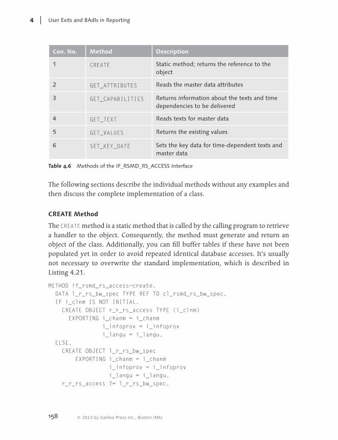
© 2013 by Galileo Press Inc., Boston (MA)158
User Exits and BAdls in Reporting4
Con. No. Method Description
1 CREATE Static method; returns the reference to the object
2 GET_ATTRIBUTES Reads the master data attributes
3 GET_CAPABILITIES Returns information about the texts and time dependencies to be delivered
4 GET_TEXT Reads texts for master data
5 GET_VALUES Returns the existing values
6 SET_KEY_DATE Sets the key data for time-dependent texts and master data
Table 4.6 Methods of the IF_RSMD_RS_ACCESS Interface
The following sections describe the individual methods without any examples and then discuss the complete implementation of a class.
CREATE Method
The CREATE method is a static method that is called by the calling program to retrieve a handler to the object. Consequently, the method must generate and return an object of the class. Additionally, you can fill buffer tables if these have not been populated yet in order to avoid repeated identical database accesses. It’s usually not necessary to overwrite the standard implementation, which is described in Listing 4.21.
METHOD if_rsmd_rs_access~create. DATA l_r_rs_bw_spec TYPE REF TO cl_rsmd_rs_bw_spec. IF i_clnm IS NOT INITIAL. CREATE OBJECT r_r_rs_access TYPE (i_clnm) EXPORTING i_chanm = i_chanm i_infoprov = i_infoprov i_langu = i_langu. ELSE. CREATE OBJECT l_r_rs_bw_spec EXPORTING i_chanm = i_chanm i_infoprov = i_infoprov i_langu = i_langu. r_r_rs_access ?= l_r_rs_bw_spec.

159
Implementing Own Read Routines for Master Data 4.5
ENDIF. ENDMETHOD.
Listing 4.21 Example of the IF_RSMD_RS_ACCESS~CREATE Method
As you can see here, an object of the CL_RSMD_RS_BW_SPEC class is created in case of doubt, that is, for all InfoObjects for which no implementation is provided. This class is delivered by SAP and is used as the standard for all InfoObjects that don’t implement their own master data read routines. If required, you can check the imple-mentation of this class to see how the reading from the master data tables is done.
SET_KEY_DATE Method
The SET_KEY_DATE method is called during the execution of a query to transfer the query key date. Here, an instance attribute, P_KEY_DATE, is populated from the called parameter. In principle, a redefinition isn’t required; the only exception is that you want to read different characteristics at different points in time. However, no application is known for which this is required.
GET_CAPABILITIES Method
The only parameter of the GET_CAPABILITIES method is a returning parameter R_S_CAPABILITIES. It contains seven individual flags (see Table 4.7) that control the properties of the InfoObject. These must be filled completely.
Name of the Flag Description FALSE TRUE
NOVALFL Characteristic doesn’t contain a check table.
‘ ’ ‘X’
TXTTABFL Text table exists. ‘0’ ‘1’
TXTTIMFL Text table is time-dependent. ‘0’ ‘1’
NOLANGU Texts are language-independent. ‘ ’ ‘X’
TXTSHFL Short text exists. ‘ ’ ‘X’
TXTMDFL Medium text exists. ‘ ’ ‘X’
TXTLGFL Long text exists. ‘ ’ ‘X’
Table 4.7 Fields of Parameter R_S_CAPABILITIES

© 2013 by Galileo Press Inc., Boston (MA)160
User Exits and BAdls in Reporting4
For InfoObject 0FISCPER, the method is implemented as shown in Listing 4.22.
METHOD IF_RSMD_RS_ACCESS~GET_CAPABILITIES. r_s_capabilities-novalfl = rs_c_false. r_s_capabilities-txttabfl = rsd_c_cnvfl-true. r_s_capabilities-txttimfl = rsd_c_cnvfl-false. r_s_capabilities-nolangu = rs_c_false. r_s_capabilities-txtshfl = rs_c_true. r_s_capabilities-txtmdfl = rs_c_true. r_s_capabilities-txtlgfl = rs_c_false. ENDMETHOD.
Listing 4.22 Example of the IF_RSMD_RS_ACCESS~GET_CAPABILITIES Method
You can see the difference between the various flags.
If you don’t want to implement the flags directly, you can also fill the corresponding fields from table RSDCHABAS which lists all InfoObjects. The implementation could look like the one shown in Listing 4.23.
METHOD IF_RSMD_RS_ACCESS~GET_CAPABILITIES. SELECT SINGLE * FROM RSDCHABAS INTO CORRESPONDING FIEDLS OF r_s_capabilities WHERE CHABASNM = ‘HAUPT_KST’ AND OBJVERS = ‘A’. ENDMETHOD.
Listing 4.23 Generic Implementation of the IF_RSMD_RS_ACCESS~GET_CAPABILITIES Method
The benefit here is that you can change the individual settings directly in the Info-Object. For this purpose, the following methods must be implemented generically so that the correct values are returned depending on the set switches.
GET_VALUES Method
The GET_VALUES method is the central method of the interface. In this method, values, texts, and, if necessary, the required attributes are returned. The method’s signature is shown in Figure 4.7.
In this method, you must implement three things. First, you must collect all allowed values. For this purpose, SAP usually creates a _VALUES_GENERATE method, which returns the desired values in table E_T_CHAVLINFO. If you implement the class yourself, you should use the same name for the method.

161
Implementing Own Read Routines for Master Data 4.5
Figure 4.7 Signature of the GET_VALUES Method
The tables, which must be filled in the method, are an important aspect in the method’s interface. E_T_CHAVLINFO contains the characteristic values and the corre-sponding texts, while E_TX_ATR comprises the corresponding attributes. To maintain performance you should note the following:
EE Table I_T_SELOPT contains selection options. Only characteristic values meeting the conditions should be returned.
EE Parameter I_MAXROWS contains the number of values returned. If possible, this number of values should not be exceeded.
EE Table I_TS_REQ_ATR contains the requested attributes. No additional attributes should be returned.
When the values have been determined, you must enrich them with texts and attributes. To do so, you can call methods GET_ATTRIBUTES and GET_TEXT, which are described in the following. A possible implementation for this is shown in Listing 4.24. First, characteristic values are read, then texts, and finally attributes.
METHOD if_rsmd_rs_access~get_values. * First save the transferred parameters * to make them available for other methods. o_t_selopt = i_t_selopt. o_maxrows = i_maxrows. o_t_sorting = i_t_sorting. TRY. CALL METHOD _values_generate * You must implement this method yourself. You * must only fill the fields, C_CHAVL and I_READ_MODE. IMPORTING e_t_chavlinfo = e_t_chavlinfo.

© 2013 by Galileo Press Inc., Boston (MA)162
User Exits and BAdls in Reporting4
CATCH cx_rs_error . x_message(‘IF_RSMD_RS_ACCESS~GET_VALUES-01’). ENDTRY. *********************************************************** * Now, the texts are read. *********************************************************** TRY. CALL METHOD if_rsmd_rs_access~get_text * This method must be implemented/overwritten. * Create an empty implementation in case of doubt. CHANGING c_t_chavlinfo = e_t_chavlinfo. CATCH cx_rs_error . x_message(‘IF_RSMD_RS_ACCESS~GET_VALUES-02’). ENDTRY. *********************************************************** ** Now, the attributes are read, if they have been * requested. *********************************************************** IF i_ts_req_attr IS NOT INITIAL. * Have attributes been requested? TRY. CALL METHOD if_rsmd_rs_access~get_attributes * This method must be implemented/overwritten. * Create an empty implementation in case of doubt. EXPORTING i_ts_req_attr = i_ts_req_attr i_t_chavlinfo = e_t_chavlinfo RECEIVING r_tx_atr = e_tx_atr. CATCH cx_rs_error . x_message(‘IF_RSMD_RS_ACCESS~GET_VALUES-03’). ENDTRY. ENDIF. ENDMETHOD.
Listing 4.24 Example of the IF_RSMD_RS_ACCESS~GET_VALUES Method

163
Implementing Own Read Routines for Master Data 4.5
GET_TEXT Method
In the GET_TEXT method, you must enrich the characteristic attributes provided in the table with corresponding texts. Hence, the signature of this method is simple (see Figure 4.8).
Figure 4.8 Signature of the GET_TEXT Method
The only parameter of this method is table C_T_CHAVLINFO. This table contains all characteristic values, texts, and other information. The corresponding structure is shown in Table 4.8.
Con. No. Field Name Type Description
1 I_SID RSD_SID SID of the characteristic value
2 C_CHAVL RSD_CHAVL Characteristic value
3 C_NIOBJNM RSD_IOBJNM Name of the InfoObject
4 C_HIEID RSHIEID Hierarchy ID
5 I_TABIX I Row index
6 E_EXIST RS_BOOL Indicates whether value exists
7 E_CHATEXTS RS_S_TXTSML Short, medium, or long text
8 C_RC SYSUBRC Return value
9 I_READ_MODE RSDM_READ_MODE
Read mode
Table 4.8 Fields of Table C_T_CHAVLINFO
In the GET_TEXT method, it’s important to fill structure E_CHATEXTS with the fields TXTSH (short text), TXTMD (medium-length text), and TXTLG (long text). You must fill the fields that were indicated in method GET_CAPABILITIES.
GET_ATTRIBUTES Method
The GET_ATTRIBUTES method fills table R_TX_ATTR. This table contains the correspond-ing attributes for each characteristic value that is transferred in table I_T_CHAVLINFO.

© 2013 by Galileo Press Inc., Boston (MA)164
User Exits and BAdls in Reporting4
The requested attributes are transferred to the method in table I_TS_REQ_ATTR. The method’s signature is shown in Figure 4.9.
Figure 4.9 Signature of the GET_ATTRIBUTES Method
You already know the structure of table I_T_CHAVLINFO from the GET_TEXT method. Table I_TS_REQ_ATTR is a simple table that contains an InfoObject for each row. Table R_TX_ATTR contains the characteristic value, CHANM, in each row; the SID and the table of the attribute value, T_ATR, which comprises the attribute name ATTRINM; and the attribute value ATTRIVL in each row.
_VALUES_GENERATE Method
The _VALUES_GENERATE (or _VALUE_GENERATE) method isn’t contained in interface IF_RSMD_RS_ACCESS. Nevertheless, it’s contained in most classes delivered by SAP; for this reason, it’s described below.
This method is used to initially fill table E_T_CHAVLINFO, which is the only para-meter of the method. C_CHAVL is the only field of the structure that must be filled. The corresponding attributes of method GET_VALUES indicate which characteristic values must be delivered and how many.
4.5.2 Sample Implementation of a Master Data Read Class
The following sections describe in detail how you can implement a class for InfoObject HAUPT_KST that automatically contains all master data of the cost cen-ters 0COSTCENTER for which a specific flag (IST_HKST) was set in their master data. Texts and attributes are automatically read from the existing texts and attributes of 0COSTCENTER.
Creating Class ZCL_READ_HAUPT_KST
1. Call Transaction SE80.
2. Select Class/Interface, and enter the class name, “ZCL_READ_BASE_CCT” (see Figure 4.10).

165
Implementing Own Read Routines for Master Data 4.5
Figure 4.10 Creating Class ZCL_READ_BASE_CCT
3. Confirm that you want to create a new class.
4. The simplest way to receive all required attributes is to inherit class CL_RSMD_RS_BW_SPEC. For this purpose, right-click on the class name, ZCL_READ_BASE_CCT, select Change, and go to the Properties tab.
5. Click the Superclass button, and enter the “CL_RSMD_RS_BW_SPEC” class in the field below (see Figure 4.11).
Figure 4.11 Specifying the Inheritance in the Class Properties

© 2013 by Galileo Press Inc., Boston (MA)166
User Exits and BAdls in Reporting4
Creating GET_VALUES Method
To create the GET_VALUES method, proceed as follows.
1. Search the GET_VALUES method in the left-hand object list under ZCL_READ_BASE_CCT • Methods • Inherited Methods • IF_RSMD_RS_ACCESS.
2. Right-click on the GET_VALUES method and select Redefine (see Figure 4.12).
3. Select the IF_RSMD_RS_ACCESS~GET_VALUES method under ZCL_READ_BASE_CCT • Methods • Redefinitions, and insert the following code (see Listing 4.25).
Right-click toredefine.
Figure 4.12 Redefining a Method
METHOD IF_RSMD_RS_ACCESS~GET_VALUES. o_t_selopt = i_t_selopt. o_maxrows = i_maxrows. o_t_sorting = i_t_sorting. TRY. ******************************************************** * First, the characteristic values of the InfoObject * HAUPT_KST are determined.

167
Implementing Own Read Routines for Master Data 4.5
******************************************************** CALL METHOD _value_generate IMPORTING e_t_chavlinfo = e_t_chavlinfo. CATCH cx_rs_error . x_message(‘IF_RSMD_RS_ACCESS~GET_VALUES-01’). ENDTRY. ******************************************************** * Now, the texts for the characteristic values are determined. ******************************************************** TRY. CALL METHOD if_rsmd_rs_access~get_text CHANGING c_t_chavlinfo = e_t_chavlinfo. CATCH cx_rs_error . x_message(‘IF_RSMD_RS_ACCESS~GET_VALUES-02’). ENDTRY. ********************************************************* * Finally, the attributes of the InfoObject * HAUPT_KST are determined. ********************************************************* IF i_ts_req_attr IS NOT INITIAL. TRY. CALL METHOD if_rsmd_rs_access~get_attributes EXPORTING i_ts_req_attr = i_ts_req_attr i_t_chavlinfo = e_t_chavlinfo RECEIVING r_tx_atr = e_tx_atr. CATCH cx_rs_error . x_message(‘IF_RSMD_RS_ACCESS~GET_VALUES-03’). ENDTRY. ENDIF. ENDMETHOD.
Listing 4.25 Comprehensive Example of the IF_RSMD_RS_ACCESS~GET_VALUES Method

© 2013 by Galileo Press Inc., Boston (MA)168
User Exits and BAdls in Reporting4
Creating _VALUE_GENERATE Method
The _VALUE_GENERATE method is copied from class CL_RSMD_RS_BW_SPEC and cor-responds to the _VALUES_GENERATE method used in other classes. It is redefined in a manner analogous to the GET_VALUES method and is created as described in Listing 4.26.
METHOD _VALUE_GENERATE. DATA: l_s_costcenter TYPE /bi0/mcostcenter, l_s_chavlinfo TYPE rsdm_s_chavlinfo. * Read data in buffers. In a real implementation * Table l_s_costcenter should be created as a * static attribute to the class. SELECT * FROM /BI0/MCOSTCENTER INTO l_s_costcenter UP TO o_maxrows ROWS WHERE DATEFROM <= sy-datum AND DATETO >= sy-datum AND /BIC/IST_HKST = ‘X’. * Set read mode now l_s_chavlinfo-i_read_mode = rsdm_c_read_mode-text. * Because HAUPT_KST is compounded to 0CO_AREA (analogous to * 0COSTCENTER), the key must be composed here. CONCATENATE l_s_costcenter-co_area l_s_costcenter-costcenter INTO l_s_chavlinfo-c_chavl. INSERT l_s_chavlinfo INTO TABLE e_t_chavlinfo. ENDSELECT. IF sy-subrc <> 0. RAISE EXCEPTION TYPE cx_rs_error. ENDIF. ENDMETHOD.
Listing 4.26 Comprehensive Example of the _VALUE_GENERATE Method
Creating GET_ATTRIBUTES Method
Analogous to the previous methods, the GET_ATTRIBUTES method is implemented as follows (see Listing 4.27). Here, the master data of the cost centers is read from the view to attribute table /BI0/MCOSTCENTER. For the sake of simplicity, time-dependency is ignored here, and only the currently valid value is read. Then, the attributes, 0PROFIT_CTR and 0RESP_PERS, are transferred to the return table, R_TX_ATR.
METHOD IF_RSMD_RS_ACCESS~GET_ATTRIBUTES. **TRY.

169
Implementing Own Read Routines for Master Data 4.5
*CALL METHOD SUPER->IF_RSMD_RS_ACCESS~GET_ATTRIBUTES * EXPORTING ** i_ts_req_attr = * I_T_CHAVLINFO = * RECEIVING * R_TX_ATR = * . ** CATCH cx_rs_error . **ENDTRY. FIELD-SYMBOLS: <f_chavl> TYPE RSDM_S_CHAVLINFO, <f_mcctr> TYPE /bi0/mcostcenter. DATA: l_t_mcctr TYPE HASHED TABLE OF /bi0/mcostcenter WITH UNIQUE KEY co_area costcenter INITIAL SIZE 0. DATA: l_sx_atr TYPE rsdm_sx_atr, l_s_atr TYPE rsdm_s_atr. * Here as well, Table l_t_mcctr should be outsourced in a * static attribute of the class and filled in the * CREATE routine. SELECT * FROM /bi0/mcostcenter INTO TABLE l_t_mcctr WHERE dateto >= sy-datum AND datefrom <= sy-datum. * Now, all characteristics to be filled are read LOOP AT i_t_chavlinfo ASSIGNING <f_chavl>. READ TABLE l_t_mcctr ASSIGNING <f_mcctr> WITH TABLE KEY co_area = <f_chavl>-c_chavl(4) costcenter = <f_chavl>-c_chavl+4(10). IF sy-subrc = 0. * Now, Return Table R_TX_ATR is filled l_sx_atr-chavl = <f_chavl>-c_chavl. REFRESH l_sx_atr-t_atr. * Fill profit center l_s_atr-attrinm = ‘0PROFIT_CTR’. l_s_atr-attrivl = <f_mcctr>-profit_ctr. INSERT l_s_atr INTO TABLE l_sx_atr-t_atr. * Fill person responsible l_s_atr-attrinm = ‘0RESP_PERS’.

© 2013 by Galileo Press Inc., Boston (MA)170
User Exits and BAdls in Reporting4
l_s_atr-attrivl = <f_mcctr>-resp_pers. INSERT l_s_atr INTO TABLE l_sx_atr-t_atr. INSERT l_sx_atr INTO TABLE r_tx_atr. ENDIF. ENDLOOP. ENDMETHOD.
Listing 4.27 Comprehensive Example of the IF_RSMD_RS_ACCESS~GET_CAPABILITIES Method
Creating GET_TEXT Method
The GET_TEXT method is implemented as shown in Listing 4.28. For the determined cost centers, the texts from text table /BI0/TCOSTCENTER are read and filled into the fields of structure E_CHATEXTS.
METHOD IF_RSMD_RS_ACCESS~GET_TEXT. **TRY. *CALL METHOD SUPER->IF_RSMD_RS_ACCESS~GET_TEXT * CHANGING * C_T_CHAVLINFO = * . ** CATCH cx_rs_error . **ENDTRY. FIELD-SYMBOLS: <f_chavl> TYPE RSDM_S_CHAVLINFO, <f_tcctr> TYPE /bi0/tcostcenter. DATA: l_t_tcctr TYPE HASHED TABLE OF /bi0/tcostcenter WITH UNIQUE KEY co_area costcenter INITIAL SIZE 0. SELECT * FROM /bi0/tcostcenter INTO TABLE l_t_tcctr WHERE dateto >= sy-datum AND datefrom <= sy-datum AND langu = sy-langu. LOOP AT c_t_chavlinfo ASSIGNING <f_chavl>. READ TABLE l_t_tcctr ASSIGNING <f_tcctr> WITH TABLE KEY co_area = <f_chavl>-c_chavl(4) costcenter = <f_chavl>-c_chavl+4(10). IF sy-subrc = 0. <f_chavl>-e_chatexts-txtsh = <f_tcctr>-txtsh.

171
Implementing Own Read Routines for Master Data 4.5
<f_chavl>-e_chatexts-txtmd = <f_tcctr>-txtmd. ENDIF. ENDLOOP. ENDMETHOD.
Listing 4.28 Comprehensive Example of the IF_RSMD_RS_ACCESS~GET_TEXT Method
4.5.3 Entering the Class in the InfoObject
You must change the InfoObject BASE_CCT.
1. Call InfoObject BASE_CCT.
2. The Master Data/Texts tab contains the field Master Data Access. In this field, select Own Implementation (see Figure 4.13).
Figure 4.13 Entering the Master Data Read Class in the InfoObject
3. Select the name of the master data read class, ZCL_READ_BASE_CCT.

© 2013 by Galileo Press Inc., Boston (MA)172
User Exits and BAdls in Reporting4
InfoObjects with Master Data Class
InfoObjects with master data read classes can’t have any navigation attributes. Moreover, the master data maintenance doesn’t read the results of the master data read class.
4. After you’ve activated the InfoObject, you can test the implementation. The simplest way to do this is to call the master data maintenance and use (F4) in the InfoObject.
At this point, you can set a clean breakpoint to debug any possible errors.
In general, creating your own master data read class is a nice alternative to imple-menting effects that would not be possible otherwise (for example, automatic filtering or user-dependent texts). However, you should always check whether it would make more sense to load the InfoObject conventionally.
It’s recommended that you implement the master data read classes only in excep-tional cases. Particularly, the restriction that InfoObjects mustn’t contain navigation attributes doesn’t allow for their widespread use.

173
5 User Exits in Planning
The biggest strength of planning in SAP NetWeaver Business Warehouse is the option to manipulate the dataset stored in the InfoProvider by means of the planning function. Some customers use this option to correct actual data retrospectively if corrections cannot be done in the SAP ERP system due to closed periods. The data-sets can also be corrected retrospectively if errors are found in the transformations.
In general, there are three different types of exits in planning:
EE Variables that function analogous to query variables
EE Characteristic derivations to derive fields that don’t exist in the planning inter-face directly
EE Specifically written functions
This list also indicates the order of complexity. Variables have a relatively simple programming; functions, however, feature a rather complex implementation and are very powerful.
The following sections describe the various types of exits and offer examples of their implementations in SAP NetWeaver BW Business Planning and Simulation (SAP BW-BPS) and in SAP NetWeaver BW Integrated Planning. You’ll discover that the actual logic remains unchanged despite completely different interfaces: SAP BW-BPS usually includes function modules, whereas SAP NetWeaver BW Integrated Planning uses classes. This makes it relatively easy to continue to use the existing modules after a migration without having to implement all functions anew.
5.1 Variables in Planning
SAP BW-BPS and SAP NetWeaver BW Integrated Planning vary considerably with regard to variables because the variables and exits used in Business Explorer (BEx) continued to be used due to the integration of the planning layout with the query. Therefore, the following sections mainly discuss the variables of SAP BW-BPS. For further information on SAP NetWeaver BW Integrated Planning, refer to Section 4.1.

© 2013 by Galileo Press Inc., Boston (MA)174
User Exits in Planning5
5.1.1 Variables in SAP BW-BPS
The variable concept in SAP BW-BPS is completely different from the variable con-cept in BEx and in SAP NetWeaver BW Integrated Planning. Hence, you’re provided with a brief introduction to this concept, which is followed by a description of the actual implementation.
In the variable exit of reporting, you directly fill the attributes to be used in the report. In contrast, in the variables in SAP BW-BPS, the permitted attributes are filled by means of exits, and the user may select a value. This stands in contrast to the variables in BEx, which either can be filled completely without user input or the user can select any valid value. If the value isn’t permitted in a specific context, a message is sent.
Another difference is that variables are saved across sessions. You can display the current variable values in Transaction BPS0 by clicking the Set Variables button (see Figure 5.1).
Figure 5.1 Setting Variables in SAP BW-BPS
However, this may result in some undesirable side effects. If an exit reads the value of another variable to determine the variable value, the developers cannot establish whether this other variable is used at all.

175
Variables in Planning 5.1
Use of Variables for Car Dealers
Let’s assume that you’re responsible for planning car sales, and your planning includes an InfoObject for brands and another InfoObject for models. If you select a brand, the exit is supposed to provide all possible models of the brand currently available. Therefore, you first read the variable of the brand and determine the models accordingly.
It may be possible, however, that you use the variables for the models at the planning level, which contains all brands. Then, your exit would still read the variable of the brand, although it isn’t used in the current context. Effects like these often result in a large number of variables and planning levels, that is, parts of InfoProvider data for which you run your functions.
If you take these cases into account for the implementation of variables, the actual exit can be implemented easily. It consists of a function module with a fixed inter-face. This function module can then be entered in one or more variables. Note that within the function module, the different variables are considered.
Similar to the variables for reporting, a distinction is made for variables that return values dependent and independent of other variable values. In the following sec-tions, you will learn more about the difference between returning single values and returning value sets.
Example 1: Returning a Single Value without Dependency of Other Variables
The example shown in Listing 5.1 assumes that different kinds of planning are implemented in the course of a year (medium-term planning, annual planning, forecast) that all use the same layouts (which are the planning input screens) and planning levels. To avoid having to change all planning levels prior to every plan-ning session, you want to enter the plan version in a central table. The version is read from this table and returned to it.
FUNCTION Z_VAR_VAL_PLANVERSION. *”------------------------------------------------------ *”*”Local interface: *” IMPORTING *” VALUE(I_AREA) TYPE UPC_Y_AREA *” VALUE(I_VARIABLE) TYPE UPC_Y_VARIABLE *” VALUE(I_CHANM) TYPE UPC_Y_CHANM OPTIONAL *” VALUE(ITO_CHANM) TYPE UPC_YTO_CHA *” EXPORTING *” REFERENCE(ETO_CHARSEL) TYPE UPC_YTO_CHARSEL

© 2013 by Galileo Press Inc., Boston (MA)176
User Exits in Planning5
*” EXCEPTIONS *” FAILED *”------------------------------------------------------ * Input parameter: * i_area : Planning area, in which the variable * is defined. * i_variable : Variable name. * i_chanm : As of Release 3.0B, the variables were * extended and can contain more than one * characteristic(in Release 3.0A, only one was * contained). To maintain the existing exits * parameter i_chanm is filled if the variables * only contain one characteristic. * ito_chanm : The table of characteristics for which the * variable was defined. It is always filled * independent of the number of characteristics. * Export parameter : * eto_charsel : Selection table for the variable in * Structure upc_ys_charsel * Exceptions: * Exceptions in the Exit function module can be output * using the message ... raising <exception name> command. * All exceptions can be used and the error is * captured. * ------------------------------------------------------ * The structure * UPC_YS_CHARSEL * Fields: CHANM - Characteristic * SEQNO – Sequential number * SIGN - I/E for Include/Exclude * OPT - Selection condition (EQ, BT, ...) * LOW - Lower limit or single value * HIGH - Upper limit * ------------------------------------------------------ DATA l_eto_charsel_wa TYPE upc_ys_charsel. DATA: l_t_plan_zentra TYPE STANDARD TABLE OF z_plan_zentra, wa_plan_zentra TYPE z_plan_zentra, l_d_version TYPE /bi0/oiversion.

177
Variables in Planning 5.1
* CLEAR export table CLEAR eto_charsel. *Transparent table read with key from column ZV SELECT * FROM z_plan_zentra INTO TABLE l_t_plan_zentra. READ TABLE l_t_plan_zentra INTO wa_plan_zentra WITH KEY ZZ_PLAN = ‚PLN’. IF sy-subrc NE 0. ENDIF. l_d_version = wa_nbw_zentra-ZZ_VERSion. * Fill selection condition l_eto_charsel_wa-chanm = i_chanm. l_eto_charsel_wa-seqno = ‘0001’. l_eto_charsel_wa-sign = ‘I’. l_eto_charsel_wa-opt = ‘EQ’. l_eto_charsel_wa-low = l_d_version. l_eto_charsel_wa-high = ‘ ’. INSERT l_eto_charsel_wa INTO TABLE eto_charsel. * Check InfoObject IF i_chanm IS INITIAL OR i_chanm NE ‘0VERSION’. * Error occurred in user exit for variables Message e538(upc) raising FAILED. ENDIF. ENDFUNCTION.
Listing 5.1 Example of BPS Variable Delivering a Single Value
Example 2: Returning a Value Set without Dependency of Other Variables
The example shown in Listing 5.2 indicates how you can use variables for imple-menting time-dependent validities. The example assumes that the planning is based on the characteristic of the product group PRODGRP, that the product groups change frequently, and that they aren’t available for planning all of the time. For this reason, there are two attributes, VALIDFROM and VALIDTO, that indicate whether a product group is currently valid.
The basic idea is to read all values that are valid for the year to be planned, that is, for which “Valid from” is smaller or equal to the last day of the year, and “Valid to” is larger or equal to the first day of the year.

© 2013 by Galileo Press Inc., Boston (MA)178
User Exits in Planning5
If you select the Restriction of Values Required by User option when you create the variable, you can select from these values. However, for planning functions, such as the pre-assignment of planning, it may be useful to restrict to the entire value set. This enables you to pre-assign only those product groups that are actually planned.
FUNCTION Z_VALID_PRODGRP. *”------------------------------------------------------ *”*”Local interface: *” IMPORTING *” REFERENCE(I_AREA) TYPE UPC_Y_AREA *” REFERENCE(I_VARIABLE) TYPE UPC_Y_VARIABLE *” REFERENCE(I_CHANM) TYPE UPC_Y_CHANM *” REFERENCE(ITO_CHANM) TYPE UPC_YTO_CHA *” EXPORTING *” REFERENCE(ETO_CHARSEL) TYPE UPC_YTO_CHARSEL *”------------------------------------------------------ * DATA: lto_chasel TYPE upc_yto_chasel, lto_chasel_wa TYPE upc_ys_chasel, lto_attr_chasel TYPE upc_yt_charng, lto_attr_chasel_wa TYPE upc_ys_charng. FIELD-SYMBOLS: <f_chasel> TYPE upc_ys_charsel. DATA: r_var TYPE REF TO cl_sem_variable, rr_variable TYPE REF TO cl_sem_variable, lto_value TYPE upc_yto_charsel, ls_value like line of lto_value, l_d_var type upc_y_variable. DATA: ltr_prodgrp TYPE HASHED TABLE OF /bic/pprodgrp WITH UNIQUE KEY /bic/prodgrp, l_s_prodgrp TYPE /bic/pprodgrp, l_d_jahr TYPE /bi0/oifiscyear, l_d_last_datefrom type d, l_d_first_dateto type d. DATA: leto_chavl TYPE upc_yto_chavl. DATA: ltmp_s_chavl TYPE upc_ys_chavl, leto_charsel_wa TYPE upc_ys_charsel. SELECT SINGLE jahr FROM z_plan_zentra into l_d_jahr WHERE zz_plan_runde = ‘ZV’.

179
Variables in Planning 5.1
l_d_last_datefrom(4) = l_d_jahr. l_d_last_datefrom+4(4) = ‘1231’. l_d_first_dateto(4) = l_d_jahr. l_d_first_dateto+4(4) = ‘0101’. * Write characteristic values in selection table leto_charsel_wa-seqno = 0. SELECT * FROM /bic/pprodgrp INTO l_s_prodgrp. WHERE /bic/validfrom <= l_d_last_datefrom AND /bic/validto <= l_d_first_dateto. leto_charsel_wa-chanm = ‘PRODGRP’. leto_charsel_wa-sign = ‘I’. leto_charsel_wa-opt = ‘EQ’. leto_charsel_wa-low = l_s_prodgrp-/bic/prodgrp. READ TABLE eto_charsel TRANSPORTING NO FIELDS WITH KEY low = l_s_prodgrp-/bic/prodgrp. IF sy-subrc <> 0. ADD 1 to leto_charsel_wa-seqno. INSERT leto_charsel_wa INTO TABLE eto_charsel. ENDIF. ENDSELECT. ENDFUNCTION.
Listing 5.2 Example of a Variable Returning a Value Set
Example 3: Returning a Value Set Depending on a User Variable
The example shown in Listing 5.2 is extended in Listing 5.3. You can use another variable in planning, such as 0DIVISION, if the number of product groups is still too high to enable a reasonable search. The following example reads only the values to which the user restricted the DIVISION variable and provides those product groups that have the corresponding attribute. It can always be assumed that the user has not restricted to one unique value but to several or all values. The results of the variable are read in a RANGES table.
FUNCTION Z080N_NBW_TYPKL_AUS_AG_SPAR. *”--------------------------------------------------------- *”*”Local interface: *” IMPORTING *” REFERENCE(I_AREA) TYPE UPC_Y_AREA *” REFERENCE(I_VARIABLE) TYPE UPC_Y_VARIABLE

© 2013 by Galileo Press Inc., Boston (MA)180
User Exits in Planning5
*” REFERENCE(I_CHANM) TYPE UPC_Y_CHANM *” REFERENCE(ITO_CHANM) TYPE UPC_YTO_CHA *” EXPORTING *” REFERENCE(ETO_CHARSEL) TYPE UPC_YTO_CHARSEL *”--------------------------------------------------------- DATA: lto_chasel TYPE upc_yto_chasel, lto_chasel_wa TYPE upc_ys_chasel, lto_attr_chasel TYPE upc_yt_charng, lto_attr_chasel_wa TYPE upc_ys_charng. FIELD-SYMBOLS: <f_chasel> TYPE upc_ys_charsel. DATA: r_var TYPE REF TO cl_sem_variable, rr_variable TYPE REF TO cl_sem_variable, lto_value TYPE upc_yto_charsel, ls_value like line of lto_value, l_d_var type upc_y_variable. DATA: ltr_division TYPE RANGE of /bi0/oidivision, l_s_division like line of ltr_division, ltr_prodgrp TYPE HASHED TABLE OF /bic/pprodgrp WITH UNIQUE KEY /bic/prodgrp, l_s_prodgrp TYPE /bic/pprodgrp, l_d_jahr TYPE /bi0/oifiscyear, l_d_last_datefrom type d, l_d_first_dateto type d. DATA: leto_chavl TYPE upc_yto_chavl. * Read division from variable CALL METHOD cl_sem_variable=>get_instance EXPORTING * Specify area i_area = i_area * Specify variable i_variable = ‚VSPARTE’ RECEIVING rr_variable = r_var EXCEPTIONS not_existing = 1 OTHERS = 2. CALL METHOD r_var->get_value RECEIVING

181
Variables in Planning 5.1
rto_value = lto_value EXCEPTIONS error = 1 OTHERS = 2. * ** LOOP AT lto_value INTO ls_value. l_s_division-sign = ls_value-sign. l_s_division-option = ls_value-opt. l_s_division-low = ls_value-low. l_s_division-high = ls_value-high. INSERT l_s_division INTO TABLE ltr_division. ENDLOOP. DATA: ltmp_s_chavl TYPE upc_ys_chavl, leto_charsel_wa TYPE upc_ys_charsel. SELECT SINGLE zz_jahr FROM z080n_nbw_zentra into l_d_jahr WHERE zz_plan_runde = ‚ZV’. l_d_last_datefrom(4) = l_d_jahr. l_d_last_datefrom+4(4) = ‚1231’. l_d_first_dateto(4) = l_d_jahr. l_d_first_dateto+4(4) = ‚0101’. * Write characteristic values in selection table leto_charsel_wa-seqno = 0. SELECT * FROM /bic/pprodgrp INTO l_s_prodgrp. WHERE /bic/validfrom <= l_d_last_datefrom AND /bic/validto <= l_d_first_dateto AND division IN ltr_division. leto_charsel_wa-chanm = ‚PRODGRP’. leto_charsel_wa-sign = ‚I’. leto_charsel_wa-opt = ‚EQ’. leto_charsel_wa-low = l_s_prodgrp-/bic/prodgrp. READ TABLE eto_charsel TRANSPORTING NO FIELDS WITH KEY low = l_s_prodgrp-/bic/prodgrp. IF sy-subrc <> 0. ADD 1 to leto_charsel_wa-seqno. INSERT leto_charsel_wa INTO TABLE eto_charsel. ENDIF. ENDSELECT. ENDFUNCTION.
Listing 5.3 Example of Reading BPS Variables in Other Variables

© 2013 by Galileo Press Inc., Boston (MA)182
User Exits in Planning5
5.1.2 Variables in SAP NetWeaver BW Integrated Planning
The variables in SAP NetWeaver BW Integrated Planning have been described in Chapter 4. These are the same variables that are used in the query creation. However, it often happens that SAP NetWeaver BW Integrated Planning and old SAP BW-BPS planning functions need to be integrated and implemented. This section provides the information you need to read SAP BW-BPS variables for processing variables of SAP NetWeaver BW Integrated Planning and to set SAP BW-BPS variables. In this context, it’s important to understand that only SAP BW-BPS variables can store values user-dependently. This isn’t possible for the variables in SAP NetWeaver BW Integrated Planning.
Example 4: Reading SAP BW-BPS Variables in the Query Variable Exit
As a general rule, you should map SAP BW-BPS variables on a 1:1 basis to avoid confusions. Consequently, the naming conventions should be selected in such a way that the name of the SAP BW-BPS variable is identical to the name of the BEx variable. The code shown in Listing 5.4 provides the content of the SAP BW-BPS variable for all variables starting with “BPS.”
INCLUDE zxrsru01. ... IF i_vnam(3) = ‘BPS’ DATA: l_s_variable TYPE UPC_Y_VARIABLE, L_s_area = upc_y_area. DATA: r_var TYPE REF TO cl_sem_variable, lto_value TYPE upc_yto_charsel, l_s_value LIKE LINE OF lto_value. L_s_area = ‘DEMOAREA’. L_s_variable = i_vnam. CALL METHOD cl_sem_variable=>get_instance EXPORTING * Specify area i_area = l_s_area * Specify variable i_variable = l_s_variable RECEIVING rr_variable = r_var EXCEPTIONS not_existing = 1 OTHERS = 2.

183
Variables in Planning 5.1
CALL METHOD r_var->get_user_restriction * EXPORTING * I_USER = SY-UNAME RECEIVING rto_value = lto_value. IF lines( lto_value ) = 0. CALL METHOD r_var->get_value * EXPORTING * I_USER = SY-UNAME * I_RESTRICT = ‘X’ receiving rto_value = lto_value EXCEPTIONS ERROR = 1 others = 2 . IF sy-subrc <> 0. * MESSAGE ID SY-MSGID TYPE SY-MSGTY NUMBER SY-MSGNO * WITH SY-MSGV1 SY-MSGV2 SY-MSGV3 SY-MSGV4. ENDIF. ENDIF. *** LOOP AT lto_value INTO l_s_value. move-corresponding l_s_value TO l_s_range. APPEND l_s_range TO e_t_range. ENDLOOP.
Listing 5.4 Transferring BPS Variables to IP Variables
This example assumes that all variables are defined as selection option variables, that is, as variables that can contain several single values and intervals as well as inclusions and exclusions. If you’re sure that the variable is restricted to a single value, you can adapt the code accordingly. You must consider, however, that a default value is set in case of doubt because the SAP BW-BPS variable is usually filled when the user calls an SAP BW-BPS application. If a user carries out a BW query without having implemented an SAP BW-BPS application, he receives an error message stating that the single value variable isn’t clearly restricted.

© 2013 by Galileo Press Inc., Boston (MA)184
User Exits in Planning5
Example 5: Writing SAP BW-BPS Variables in the Query Variable Exit
If BPS planning sequences are to be started from a BW query, it may be necessary to write back the BEx variables to the SAP BW-BPS variables. You can use Step 3 of the variable exit (I_STEP = 3) to write back the SAP BW-BPS variable. During this step, all variable values—both the exit variables and the normal input variables—are transferred to the exit so that you can access all variables. You can use Listing 5.5 to search for all variables starting with “BPS” and to transfer the variable value to the relevant SAP BW-BPS variable using SAP BW-BPS-API—that is, the SAP BW-BPS programming interface.
IF i_step = 3. data: l_s_bps_var TYPE UPC_YS_API_VARSEL, l_t_bps_var TYPE STANDARD TABLE OF UPC_YS_API_VARSEL. LOOP AT i_t _var_range INTO l_s_var_range. IF l_s_var_range-vnam(3) = ‘NBW’. REFRESH l_t_bps_var. CLEAR l_s_bps_var. MOVE-CORRESPONDING l_s_var_range TO l_s_bps_var. l_s_bps_var-option = l_s_var_range-opt. l_s_bps_var-chanm = l_s_var_range-iobjnm. l_s_bps_var-seqno = 1. INSERT l_s_bps_var INTO TABLE l_t_bps_var. CALL FUNCTION ‘API_SEMBPS_VARIABLE_SET’ EXPORTING I_AREA = ‘DEMOAREA’ I_VARIABLE = l_s_var_range-vnam * I_NUMVALUE = * IS_HIESEL = * IMPORTING * E_SUBRC = * ES_RETURN = TABLESw ITK_VARSEL = l_t_bps_var * ITK_HIEDEP = . ENDIF. ENDLOOP. ENDIF.
Listing 5.5 Writing Back Query Variables to BPS Variables
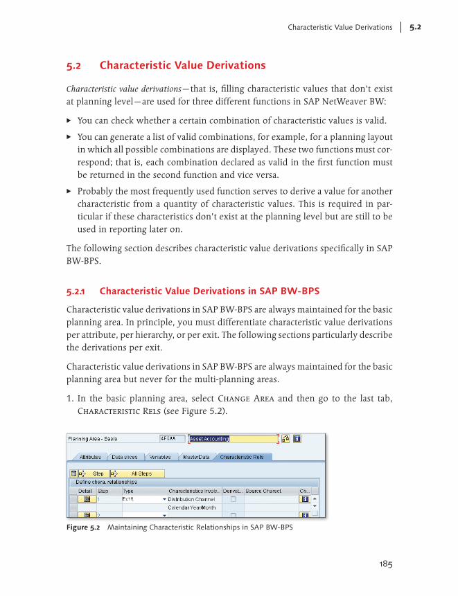
185
Characteristic Value Derivations 5.2
5.2 Characteristic Value Derivations
Characteristic value derivations—that is, filling characteristic values that don’t exist at planning level—are used for three different functions in SAP NetWeaver BW:
EE You can check whether a certain combination of characteristic values is valid.
EE You can generate a list of valid combinations, for example, for a planning layout in which all possible combinations are displayed. These two functions must cor-respond; that is, each combination declared as valid in the first function must be returned in the second function and vice versa.
EE Probably the most frequently used function serves to derive a value for another characteristic from a quantity of characteristic values. This is required in par-ticular if these characteristics don’t exist at the planning level but are still to be used in reporting later on.
The following section describes characteristic value derivations specifically in SAP BW-BPS.
5.2.1 Characteristic Value Derivations in SAP BW-BPS
Characteristic value derivations in SAP BW-BPS are always maintained for the basic planning area. In principle, you must differentiate characteristic value derivations per attribute, per hierarchy, or per exit. The following sections particularly describe the derivations per exit.
Characteristic value derivations in SAP BW-BPS are always maintained for the basic planning area but never for the multi-planning areas.
1. In the basic planning area, select Change Area and then go to the last tab, Characteristic Rels (see Figure 5.2).
Figure 5.2 Maintaining Characteristic Relationships in SAP BW-BPS

© 2013 by Galileo Press Inc., Boston (MA)186
User Exits in Planning5
2. Select the derivation type Exit.
3. Click on the first column, Detail, to navigate to the screen displayed in Figure 5.3.
4. You have two options. You can select a combination check and a combination proposal, or you can select a derivation with combination check and combina-tion proposal. In the former case, you must select the characteristics for the combination check; in the latter, you must select the source and target charac-teristics.
Figure 5.3 Details of a Characteristic Relationship in SAP BW-BPS
5. In the lower part of the screen, you can set up two or three function modules depending on the variant. SAP BW-BPS provides three different modules for the characteristic value derivations per exit: UPF_TIME_EXIT_FISC_CHECK, UPF_TIME_EXIT_FISC_CREATE, and UPF_TIME_EXIT_FISC_DERIVE. UPF_TIME_EXIT_FISC_CHECK is used for the combination check, UPF_TIME_EXIT_FISC_CREATE for the combi-nation proposal, and UPF_TIME_EXIT_FISC_DERIVE for the characteristic value derivation.
The following sections discuss the check of characteristic value combinations.
Example 6: Checking Characteristic Value Combinations in SAP BW-BPS
Initially, the characteristic value combinations are checked: This exit is called once per data record after new planning records have been created. The characteristics to be checked are entered in the definition of the characteristic value derivation.

187
Characteristic Value Derivations 5.2
For the sake of simplicity, you should select a characteristic value derivation per hierarchy or attribute derivation whenever possible. However, this isn’t possible for more complex combinations.
Listing 5.6 continues the example from Section 5.1.1. There is a product group (PRODGRP) that includes the following attributes: division (0DIVISION), a “Valid from” date (VALIDFROM), and a “Valid to” date (VALIDTO). In the exit, you now want to check whether the month is within the validity period for a product group, a calendar year, and a calendar month. If this isn’t the case, you must trigger the exception INVALID.
FUNCTION Z_DERIVE_PRODGRP_CHECK. *”--------------------------------------------------------- *”*”Local interface: *” IMPORTING *” REFERENCE(I_AREA) TYPE UPC_Y_AREA *” REFERENCE(IS_CHAS) TYPE ANY *” REFERENCE(ITO_CHA) TYPE UPC_YTO_CHA *” REFERENCE(ITO_CHASEL) TYPE UPC_YTO_CHASEL OPTIONAL *” EXCEPTIONS *” FAILED *” INVALID *”--------------------------------------------------------- FIELD-SYMBOLS: <f_prodgrp> TYPE /bic/oiprodgrp, <f_year> TYPE /bi0/oifiscyear, <f_per3> TYPE /bi0/oifiscper3, <f_chas> TYPE ANY. DATA: l_s_prodgrp like line of g_t_prodgrp, l_d_valid type c, l_d_min_to type d, l_d_max_from type d. * First, the required fields of the structure * are assigned to field symbols. ASSIGN COMPONENT ‘PRODGRP’ OF STRUCTURE is_chas TO <f_prodgrp>. ASSIGN COMPONENT ‘0FISCPER3’ OF STRUCTURE is_chas TO <f_per3>. ASSIGN COMPONENT ‘0FISCYEAR’ OF STRUCTURE is_chas TO <f_year>.

© 2013 by Galileo Press Inc., Boston (MA)188
User Exits in Planning5
IF lines( g_t_prodgrp ) = 0. SELECT * FROM /bic/pprodgrp INTO TABLE g_t_prodgrp WHERE OBJVERS = ‘A’. ENDIF. l_d_valid = ‘-’. LOOP AT g_t_prodgrp into l_s_prodgrp WHERE /bic/prodgrp = <f_prodgrp> AND OBJVERS = ‘A’. * Record valid? l_d_min_to(4) = l_d_max_from(4) = <f_year>. IF <f_per3> > ‘012’ OR <f_per3> = ‘000’. * Only check year l_d_min_to+4(4) = ‘1231’. l_d_max_from+4(4) = ‘0101’. ELSE. * Check period only from 1-12. l_d_max_from+4(2) = <f_per3>. l_d_max_from+6(2) = ‘01’. l_d_min_to = l_d_max_from. l_d_min_to = l_d_min_to + 31. l_d_min_to+6(2) = ‘01’. l_d_min_to = l_d_min_to - 1. ENDIF. IF l_s_typklasse-/bic/validfrom <= l_d_min_to AND l_s_typklasse-/bic/validto >= l_d_max_from. l_d_valid = ‘+’. ENDIF. ENDLOOP. IF l_d_valid = ‘-’. MESSAGE e101(z_bps) WITH <f_prodgrp> <f_per3> <f_year> * Product group &1 is &2/&3 not valid. RAISING INVALID. ENDIF. ENDFUNCTION.
Listing 5.6 Sample Check of Characteristic Value Combinations
For the function module, you can use the sample function module, UPF_TIME_EXIT_FISC_CHECK. It includes a sample implementation that you can follow.

189
Characteristic Value Derivations 5.2
Example 7: Creating Characteristic Value Combinations in SAP BW-BPS
The corresponding function is the creation of a list that comprises valid combina-tions. As described previously, you must determine these combinations as valid combinations in the other exit. The simplest option is to determine all possible combinations and call the first function module. However, this process usually takes a long time; therefore, it’s easier to determine the valid combinations directly. The corresponding function module then appears as shown in Listing 5.7. First, the product groups, fiscal years, and periods selected in planning are determined. Then, the validity periods of the product groups within the selected periods are determined, and these combinations are written to the return table.
FUNCTION z_derive_prodgrp_create. *”--------------------------------------------------------- *”*”Local interface: *” IMPORTING *” REFERENCE(I_AREA) TYPE UPC_Y_AREA *” REFERENCE(ITO_CHA) TYPE UPC_YTO_CHA *” REFERENCE(ITO_CHASEL) TYPE UPC_YTO_CHASEL OPTIONAL *” EXPORTING *” REFERENCE(ETH_CHAS) TYPE HASHED TABLE *” EXCEPTIONS *” FAILED *”--------------------------------------------------------- * Determination of valid characteristics for product group, * fiscal year, period DATA: l_s_chasel TYPE upc_ys_chasel, l_s_chas1 TYPE /1sem/_ys_chas_100demoarea, l_s_chas3 TYPE /1sem/_ys_chas_100demoar2, l_s_chas TYPE REF TO DATA, l_s_charng TYPE upc_ys_charng. FIELD-SYMBOLS: <f_prodgrp> TYPE /bic/oiprodgrp, <f_year> TYPE /bi0/oifiscyear, <f_per3> TYPE /bi0/oifiscper3, <f_varnt> TYPE /bi0/oifiscvarnt, <f_chas> TYPE ANY. DATA: l_tr_prodgrp TYPE RANGE OF /bic/oiprodgrp, l_tr_year TYPE RANGE OF /bi0/oifiscyear,

© 2013 by Galileo Press Inc., Boston (MA)190
User Exits in Planning5
l_tr_per3 TYPE RANGE OF /bi0/oifiscper3, l_sr_progrp LIKE LINE OF l_tr_prodgrp, l_sr_year LIKE LINE OF l_tr_year, l_sr_per3 LIKE LINE OF l_tr_per3. DATA: l_s_prodgrp TYPE /bic/pprodgrp, l_d_datum TYPE d, l_d_year TYPE /bi0/oifiscyear, l_d_per3 TYPE /bi0/oifiscper3, l_s_zentra TYPE z_pln_zentra. CREATE DATA l_s_chas LIKE LINE OF eth_chas. ASSIGN l_s_chas->* TO <f_chas>. * Initialization of field symbols ASSIGN COMPONENT ‘PRODGRP’ OF STRUCTURE <f_chas> TO <f_prodgrp>. ASSIGN COMPONENT ‘0FISCYEAR’ OF STRUCTURE <f_chas> TO <f_year>. ASSIGN COMPONENT ‘0FISCPER3’ OF STRUCTURE <f_chas> TO <f_per3>. ASSIGN COMPONENT ‘0FISCVARNT’ OF STRUCTURE <f_chas> TO <f_varnt>. LOOP AT ito_chasel INTO l_s_chasel. IF l_s_chasel-chanm = ‘PRODGRP’. LOOP AT l_s_chasel-t_charng INTO l_s_charng. MOVE-CORRESPONDING l_s_charng TO l_sr_prodgrp. INSERT l_sr_prodgrp INTO TABLE l_tr_prodgrp. ENDLOOP. ENDIF. IF l_s_chasel-chanm = ‘0FISCYEAR’. LOOP AT l_s_chasel-t_charng INTO l_s_charng. MOVE-CORRESPONDING l_s_charng TO l_sr_year. INSERT l_sr_year into table l_tr_year. ENDLOOP. ENDIF. IF l_s_chasel-chanm = ‘0FISCPER3’. LOOP AT l_s_chasel-t_charng INTO l_s_charng. MOVE-CORRESPONDING l_s_charng TO l_sr_per3. INSERT l_sr_per3 INTO TABLE l_tr_per3. ENDLOOP. ENDIF. ENDLOOP.

191
Characteristic Value Derivations 5.2
* Create table for year SELECT SINGLE * FROM z_plan_zentra INTO l_s_zentra WHERE zz_plan_runde = ‘ZV’. l_d_per3 = ‘000’. SELECT * FROM /bic/pprodgrp INTO l_s_prodgrp WHERE objvers = ‘A’ AND /bic/prodgrp IN l_tr_prodgrp. l_d_datum = l_s_prodgrp-/bic/validfrom. IF l_d_datum(4) < l_s_nbw_zentra-planjahr. l_d_datum(4) = l_s_nbw_zentra-planjahr. l_d_datum+4(4) = ‘0101’. ENDIF. IF l_s_prodgrp-/bic/validto(4) > l_s_plan_zentra-planjahr. l_s_typkl-/bic/validto(4) = l_s_plan_zentra-planjahr. l_s_typkl-/bic/validto+4(4) = ‘1231’. ENDIF. WHILE l_d_datum <= l_s_prodgrp-/bic/validto. * Insert periods # and 16 , if at least one * combination is valid l_d_per3+1(2) = l_d_datum+4(2). l_d_year = l_d_datum(4). if l_d_year in l_tr_year. <f_varnt> = ‘K4’. <f_prodgrp> = l_s_typkl-/bic/prodgrp. <f_year> = l_d_year. IF ‘016’ IN l_tr_per3. <f_per3> = ‘016’. INSERT <f_chas> INTO TABLE eth_chas. ENDIF. IF ‘000’ IN l_tr_per3. <f_per3> = ‘000’. INSERT <f_chas> INTO TABLE eth_chas. ENDIF. IF l_d_per3 IN l_tr_per3. * valid combination <f_prodgrp> = l_s_typkl-/bic/prodgrp. <f_year> = l_d_year. <f_per3> = l_d_per3.

© 2013 by Galileo Press Inc., Boston (MA)192
User Exits in Planning5
INSERT <f_chas> INTO TABLE eth_chas. ENDIF. ENDIF. * Increment date l_d_datum+6(2) = ‘01’. l_d_datum = l_d_datum + 31. ENDWHILE. ENDSELECT. ENDFUNCTION.
Listing 5.7 Example of the CREATE Function of the Characteristic Value Derivation
Example 8: Derivation of Characteristic Values in SAP BW-BPS
The last function of the characteristic value derivation includes the enrichment of fields that don’t exist at the planning level. You can use this option in various ways. For instance, a project may require that plan line items must be written to trace who changed which plan value and when. At first glance, this seems impossible within SAP NetWeaver BW, but with the characteristic value derivation, it can be implemented easily.1
To derive characteristics you simply include three InfoObjects for the user (0USER-NAME), date (0DATE), and time (0TIME) in the InfoCube of the planning area and fill these via the exit for the characteristic value derivation, which you program as shown in Listing 5.8. Note that you must always enter a source characteristic for the exit (for instance, the fiscal year, 0FISCYEAR).
FUNCTION Z_DERIVE_0USERNAME. *”--------------------------------------------------------- *”*”Local interface: *” IMPORTING *” VALUE(I_AREA) TYPE UPC_Y_AREA *” REFERENCE(ITO_CHA) TYPE UPC_YTO_CHA *” CHANGING *” REFERENCE(XS_CHAS) TYPE ANY *” EXCEPTIONS *” FAILED *”---------------------------------------------------------
1 This example is based on the document, “How to ... line items in SAP BW-BPS.” It was selected because it fits in this context and is easy to implement. Most of the other examples are too com-plex to be described within the scope of in this book or could be better implemented by means of attribute or hierarchy derivations.

193
Characteristic Value Derivations 5.2
FIELD-SYMBOLS: <l_chavl> TYPE ANY. * fill user ASSIGN COMPONENT ‘0USERNAME’ OF STRUCTURE xs_chas TO <l_chavl>. IF sy-subrc = 0. <l_chavl> = sy-uname. ENDIF. * fill date ASSIGN COMPONENT ‘0DATE’ OF STRUCTURE xs_chas TO <l_chavl>. IF sy-subrc = 0. <l_chavl> = sy-datum. ENDIF. *** fill time ASSIGN component ‘0TIME’ OF STRUCTURE xs_chas TO <l_chavl>. IF sy-subrc = 0. <l_chavl> = sy-uzeit. ENDIF. ENDFUNCTION.
Listing 5.8 Sample Implementation for Deriving Characteristic Values
After having introduced characteristic derivation in SAP BW-BPS, the following sec-tion deals with characteristic derivations in SAP NetWeaver BW Integrated Planning.
5.2.2 Characteristic Value Derivations in SAP NetWeaver BW Integrated Planning
The characteristic value derivation in SAP NetWeaver BW Integrated Planning functions analogously to characteristic value derivation in SAP BW-BPS; however, you must implement a class with corresponding interfaces instead of one or more function modules. Then, you must enter this class in the Planning Modeler in Transaction RSPLAN.
In many projects, you can select between SAP BW-BPS and SAP NetWeaver BW Integrated Planning or a combination of old SAP BW-BPS applications and new SAP NetWeaver BW Integrated Planning applications. For better comparability, in the following sections, the same exits as in SAP BW-BPS are implemented.
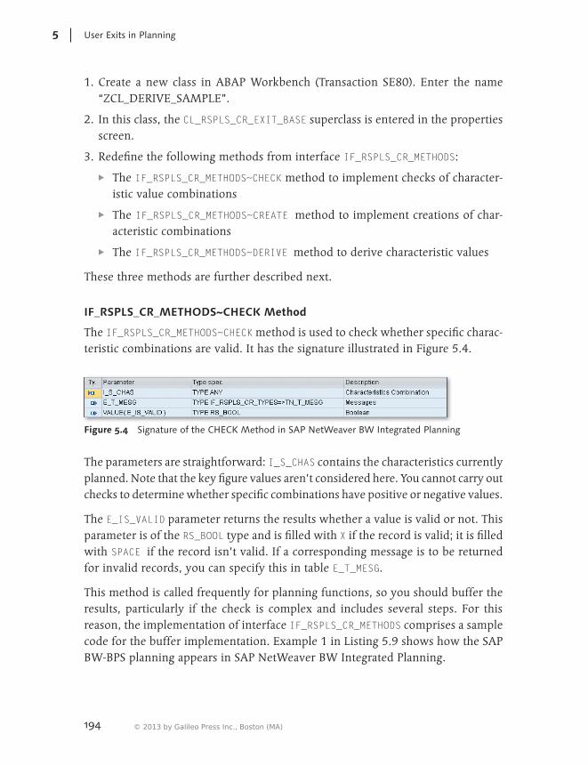
© 2013 by Galileo Press Inc., Boston (MA)194
User Exits in Planning5
1. Create a new class in ABAP Workbench (Transaction SE80). Enter the name “ZCL_DERIVE_SAMPLE”.
2. In this class, the CL_RSPLS_CR_EXIT_BASE superclass is entered in the properties screen.
3. Redefine the following methods from interface IF_RSPLS_CR_METHODS:
EE The IF_RSPLS_CR_METHODS~CHECK method to implement checks of character-istic value combinations
EE The IF_RSPLS_CR_METHODS~CREATE method to implement creations of char-acteristic combinations
EE The IF_RSPLS_CR_METHODS~DERIVE method to derive characteristic values
These three methods are further described next.
IF_RSPLS_CR_METHODS~CHECK Method
The IF_RSPLS_CR_METHODS~CHECK method is used to check whether specific charac-teristic combinations are valid. It has the signature illustrated in Figure 5.4.
Figure 5.4 Signature of the CHECK Method in SAP NetWeaver BW Integrated Planning
The parameters are straightforward: I_S_CHAS contains the characteristics currently planned. Note that the key figure values aren’t considered here. You cannot carry out checks to determine whether specific combinations have positive or negative values.
The E_IS_VALID parameter returns the results whether a value is valid or not. This parameter is of the RS_BOOL type and is filled with X if the record is valid; it is filled with SPACE if the record isn’t valid. If a corresponding message is to be returned for invalid records, you can specify this in table E_T_MESG.
This method is called frequently for planning functions, so you should buffer the results, particularly if the check is complex and includes several steps. For this reason, the implementation of interface IF_RSPLS_CR_METHODS comprises a sample code for the buffer implementation. Example 1 in Listing 5.9 shows how the SAP BW-BPS planning appears in SAP NetWeaver BW Integrated Planning.
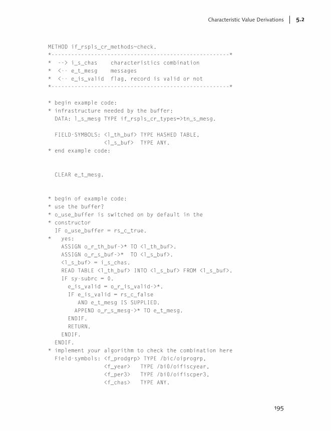
195
Characteristic Value Derivations 5.2
METHOD if_rspls_cr_methods~check. *------------------------------------------------------* * --> i_s_chas characteristics combination * <-- e_t_mesg messages * <-- e_is_valid flag, record is valid or not *------------------------------------------------------* * begin example code: * infrastructure needed by the buffer: DATA: l_s_mesg TYPE if_rspls_cr_types=>tn_s_mesg. FIELD-SYMBOLS: <l_th_buf> TYPE HASHED TABLE, <l_s_buf> TYPE ANY. * end example code: CLEAR e_t_mesg. * begin of example code: * use the buffer? * o_use_buffer is switched on by default in the * constructor IF o_use_buffer = rs_c_true. * yes: ASSIGN o_r_th_buf->* TO <l_th_buf>. ASSIGN o_r_s_buf->* TO <l_s_buf>. <l_s_buf> = i_s_chas. READ TABLE <l_th_buf> INTO <l_s_buf> FROM <l_s_buf>. IF sy-subrc = 0. e_is_valid = o_r_is_valid->*. IF e_is_valid = rs_c_false AND e_t_mesg IS SUPPLIED. APPEND o_r_s_mesg->* TO e_t_mesg. ENDIF. RETURN. ENDIF. ENDIF. * implement your algorithm to check the combination here Field-symbols: <f_prodgrp> TYPE /bic/oiprogrp, <f_year> TYPE /bi0/oifiscyear, <f_per3> TYPE /bi0/oifiscper3, <f_chas> TYPE ANY.

© 2013 by Galileo Press Inc., Boston (MA)196
User Exits in Planning5
* g_t_progrp is an attribute of the implementing class. * a hashed table with the structure /bic/prodgrp DATA: l_s_prodgrp like line of g_t_prodgrp, l_d_valid type c, l_d_min_to type d, l_d_max_from type d. ASSIGN COMPONENT ‘PRODGRP’ OF STRUCTURE i_s_chas TO <f_prodgrp>. ASSIGN COMPONENT ‘0FISCPER3’ OF STRUCTURE i_s_chas TO <f_per3>. ASSIGN COMPONENT ‘0FISCYEAR’ OF STRUCTURE i_s_chas TO <f_year>. IF lines( g_t_prodgrp ) = 0. SELECT * FROM /bic/pprodgrp INTO TABLE g_t_prodgrp WHERE OBJVERS = ‘A’. ENDIF. l_d_valid = ‘-’. LOOP AT g_t_prodgrp into l_s_prodgrp WHERE /bic/prodgrp = <f_prodgrp> AND OBJVERS = ‘A’. * Record valid? l_d_min_to(4) = l_d_max_from(4) = <f_year>. IF <f_per3> > ‘012’ OR <f_per3> = ‘000’. * Only check year l_d_min_to+4(4) = ‘1231’. l_d_max_from+4(4) = ‘0101’. ELSE. * Check period only for 1-12. l_d_max_from+4(2) = <f_per3>. l_d_max_from+6(2) = ‘01’. l_d_min_to = l_d_max_from. l_d_min_to = l_d_min_to + 31. l_d_min_to+6(2) = ‘01’. l_d_min_to = l_d_min_to - 1. ENDIF.

197
Characteristic Value Derivations 5.2
IF l_s_typklasse-/bic/validfrom <= l_d_min_to AND l_s_typklasse-/bic/validto >= l_d_max_from. l_d_valid = ‘+’. ENDIF. ENDLOOP. IF l_d_valid = ‘-’. e_is_valid = rs_c_false. l_s_mesg-msgty = ‘E’. l_s_mesg-msgid = ‘z_bps’. l_s_mesg-msgno = ‘101’. l_s_mesg-msgv1 = <f_prodgrp>. l_s_mesg-msgv2 = <f_per3>. l_s_mesg-msgv3 = <f_year>. * Product group &1 is &2/&3 not valid. APPEND l_s_mesg TO e_t_mesg. ELSE. E_is_valid = rs_c_true. ENDIF. * update the buffer with the result: * l_s_mesg should contain a message in the ‘invalid’ * case IF o_use_buffer = rs_c_true. o_r_is_valid->* = e_is_valid. IF o_r_is_valid->* = rs_c_false AND e_t_mesg IS SUPPLIED. o_r_s_mesg->* = l_s_mesg. ENDIF. INSERT <l_s_buf> INTO TABLE <l_th_buf>. ENDIF. * end of example code ENDMETHOD.
Listing 5.9 Sample Implementation of the CHECK Method
IF_RSPLS_CR_METHODS~CREATE Method
Like SAP BW-BPS, SAP NetWeaver BW Integrated Planning also includes a method, the IF_RSPLS_CR_METHODS~CREATE method, that provides all valid characteristic combinations (see Figure 5.5). The signature of this method is more complex than the signature of the CHECK method.
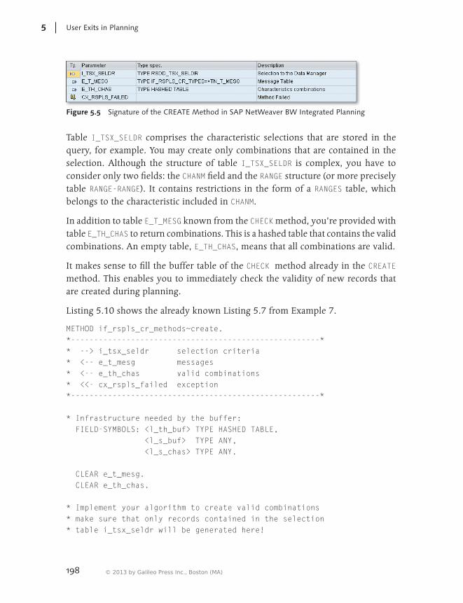
© 2013 by Galileo Press Inc., Boston (MA)198
User Exits in Planning5
Figure 5.5 Signature of the CREATE Method in SAP NetWeaver BW Integrated Planning
Table I_TSX_SELDR comprises the characteristic selections that are stored in the query, for example. You may create only combinations that are contained in the selection. Although the structure of table I_TSX_SELDR is complex, you have to consider only two fields: the CHANM field and the RANGE structure (or more precisely table RANGE-RANGE). It contains restrictions in the form of a RANGES table, which belongs to the characteristic included in CHANM.
In addition to table E_T_MESG known from the CHECK method, you’re provided with table E_TH_CHAS to return combinations. This is a hashed table that contains the valid combinations. An empty table, E_TH_CHAS, means that all combinations are valid.
It makes sense to fill the buffer table of the CHECK method already in the CREATE method. This enables you to immediately check the validity of new records that are created during planning.
Listing 5.10 shows the already known Listing 5.7 from Example 7.
METHOD if_rspls_cr_methods~create. *------------------------------------------------------* * --> i_tsx_seldr selection criteria * <-- e_t_mesg messages * <-- e_th_chas valid combinations * <<- cx_rspls_failed exception *------------------------------------------------------* * Infrastructure needed by the buffer: FIELD-SYMBOLS: <l_th_buf> TYPE HASHED TABLE, <l_s_buf> TYPE ANY, <l_s_chas> TYPE ANY. CLEAR e_t_mesg. CLEAR e_th_chas. * Implement your algorithm to create valid combinations * make sure that only records contained in the selection * table i_tsx_seldr will be generated here!

199
Characteristic Value Derivations 5.2
* Determine valid characteristics for the product group, * fiscal year, period FIELD-SYMBOLS: <f_prodgrp> TYPE /bic/oiprodgrp, <f_year> TYPE /bi0/oifiscyear, <f_per3> TYPE /bi0/oifiscper3, <f_varnt> TYPE /bi0/oifiscvarnt, <f_chas> TYPE ANY, <f_seldr> TYPE RSDD_SX_SELDR, <f_range> TYPE RRRANGESID. DATA: l_tr_prodgrp TYPE RANGE OF /bic/oiprodgrp, l_tr_year TYPE RANGE OF /bi0/oifiscyear, l_tr_per3 TYPE RANGE OF /bi0/oifiscper3, l_sr_progrp LIKE LINE OF l_tr_prodgrp, l_sr_year LIKE LINE OF l_tr_year, l_sr_per3 LIKE LINE OF l_tr_per3. DATA: l_s_prodgrp TYPE /bic/pprodgrp, l_d_datum TYPE d, l_d_year TYPE /bi0/oifiscyear, l_d_per3 TYPE /bi0/oifiscper3, l_s_zentra TYPE z_pln_zentra. CREATE DATA l_s_chas LIKE LINE OF eth_chas. ASSIGN l_s_chas->* TO <f_chas>. * Initialization of field symbols ASSIGN COMPONENT ‘PRODGRP’ OF STRUCTURE <f_chas> TO <f_prodgrp>. ASSIGN COMPONENT ‘0FISCYEAR’ OF STRUCTURE <f_chas> TO <f_year>. ASSIGN COMPONENT ‘0FISCPER3’ OF STRUCTURE <f_chas> TO <f_per3>. ASSIGN COMPONENT ‘0FISCVARNT’ OF STRUCTURE <f_chas> TO <f_varnt>. LOOP AT i_tsx_seldr ASSIGNING <f_seldr>. IF <f_seldr>-chanm = ‘PRODGRP’. LOOP AT <f_seldr>-range-range ASSIGNING <f_range>. MOVE-CORRESPONDING <f_range> TO l_sr_prodgrp. INSERT l_sr_prodgrp INTO TABLE l_tr_prodgrp. ENDLOOP. ENDIF.

© 2013 by Galileo Press Inc., Boston (MA)200
User Exits in Planning5
IF <f_seldr>-chanm = ‘0FISCYEAR’. LOOP AT <f_seldr>-range-range ASSIGNING <f_range>. MOVE-CORRESPONDING <f_range> TO l_sr_year. INSERT l_sr_year into table l_tr_year. ENDLOOP. ENDIF. IF <f_seldr>-chanm = ‘0FISCPER3’. LOOP AT <f_seldr>-range-range ASSIGNING <f_range>. MOVE-CORRESPONDING <f_range> TO l_sr_per3. INSERT l_sr_per3 INTO TABLE l_tr_per3. ENDLOOP. ENDIF. ENDLOOP. * Create table for year SELECT SINGLE * FROM z_plan_zentra INTO l_s_zentra WHERE zz_plan_runde = ‘ZV’. l_d_per3 = ‘000’. SELECT * FROM /bic/pprodgrp INTO l_s_prodgrp WHERE objvers = ‘A’ AND /bic/prodgrp IN l_tr_prodgrp. l_d_datum = l_s_prodgrp-/bic/validfrom. IF l_d_datum(4) < l_s_nbw_zentra-planjahr. l_d_datum(4) = l_s_nbw_zentra-planjahr. l_d_datum+4(4) = ‘0101’. ENDIF. IF l_s_prodgrp-/bic/validto(4) > l_s_plan_zentra-planjahr. l_s_typkl-/bic/validto(4) = l_s_plan_zentra-planjahr. l_s_typkl-/bic/validto+4(4) = ‘1231’. ENDIF. WHILE l_d_datum <= l_s_prodgrp-/bic/validto. * Insert periods # and 16 , if at least one * combination is valid l_d_per3+1(2) = l_d_datum+4(2). l_d_year = l_d_datum(4). if l_d_year in l_tr_year. <f_varnt> = ‘K4’. <f_prodgrp> = l_s_typkl-/bic/prodgrp. <f_year> = l_d_year.

201
Characteristic Value Derivations 5.2
IF ‘016’ IN l_tr_per3. <f_per3> = ‘016’. INSERT <f_chas> INTO TABLE eth_chas. ENDIF. IF ‘000’ IN l_tr_per3. <f_per3> = ‘000’. INSERT <f_chas> INTO TABLE eth_chas. ENDIF. IF l_d_per3 IN l_tr_per3. * valid combination <f_prodgrp> = l_s_typkl-/bic/prodgrp. <f_year> = l_d_year. <f_per3> = l_d_per3. INSERT <f_chas> INTO TABLE eth_chas. ENDIF. ENDIF. * Increment date l_d_datum+6(2) = ‘01’. l_d_datum = l_d_datum + 31. ENDWHILE. ENDSELECT. * Use the buffer? * o_use_buffer is switched on by default in the * constructor IF o_use_buffer = rs_c_true. * update the buffer with the created records ASSIGN o_r_th_buf->* TO <l_th_buf>. ASSIGN o_r_s_buf->* TO <l_s_buf>. LOOP AT e_th_chas ASSIGNING <l_s_chas>. <l_s_buf> = <l_s_chas>. o_r_is_valid->* = rs_c_true. INSERT <l_s_buf> INTO TABLE <l_th_buf>. ENDLOOP. ENDIF. ENDMETHOD.
Listing 5.10 Sample Implementation of the CREATE Method
IF_RSPLS_CR_METHODS~DERIVE Method
The IF_RSPLS_CR_METHODS~DERIVE method is different from the CREATE and CHECK methods because the DERIVE method addresses characteristics that aren’t at the

© 2013 by Galileo Press Inc., Boston (MA)202
User Exits in Planning5
aggregation level. These characteristics are filled using the DERIVE method. Just as in the CHECK method, it’s implemented at the level of individual records. Hence, the signature of this method is practically identical (see Figure 5.6).
Figure 5.6 Signature of the DERIVE Method in SAP NetWeaver BW Integrated Planning
Because you change characteristic values, you need to use the C_S_CHAS changing parameter instead of the I_S_CHAS importing parameter that has the same structure. Table E_T_MESG is identical to the table parameters in the CHECK and CREATE methods. Instead of the E_IS_VALID parameter of the CHECK method, you’re provided with the CX_RSPLS_FAILED exception. This exception should only be triggered if serious errors or illogical selection conditions (for example, “Valid from” is larger than “Valid to”) occur in the database because it aborts the entire planning function.
For SAP NetWeaver BW Integrated Planning, Listing 5.11 shows a derivation of user and time information taken from the SAP BW-BPS example. The only differences are the parameter names and the fact that this is a method and not a function module.
METHOD if_rspls_cr_methods~derive. *------------------------------------------------------* * <-- e_t_mesg messages * <-> c_s_chas * characteristic combination: * source and target * fields included; do not change the source fields * <<- cx_rspls_failed exception *------------------------------------------------------* CLEAR e_t_mesg. FIELD-SYMBOLS: <l_chavl> TYPE ANY. * fill user ASSIGN COMPONENT ‘0USERNAME’ OF STRUCTURE c_s_chas TO <l_chavl>. IF sy-subrc = 0. <l_chavl> = sy-uname. ENDIF. * fill date ASSIGN COMPONENT ‘0DATE’ OF STRUCTURE c_s_chas TO <l_chavl>.

203
Exit Functions in Planning 5.3
IF sy-subrc = 0. <l_chavl> = sy-datum. ENDIF. *** fill time ASSIGN COMPONENT ‘0TIME’ OF STRUCTURE c_s_chas TO <l_chavl>. IF sy-subrc = 0. <l_chavl> = sy-uzeit. ENDIF. ENDMETHOD.
Listing 5.11 Sample Implementation of the DERIVE Method
The examples above illustrate that the different methods can be easily adapted to your concrete usage scenario. You can even call the original function module if you want to transform a project from SAP BW-BPS to SAP NetWeaver BW Integrated Planning.
5.3 Exit Functions in Planning
This section presents the most powerful planning tool—the exit function. In both SAP BW-BPS and in SAP NetWeaver BW Integrated Planning, you can manipulate the entire dataset via an exit.
5.3.1 Exit Functions in SAP BW-BPS
Exit functions in SAP BW-BPS are an essential part of many BPS implementations. The function to manipulate entire sets of data offers many opportunities that should not be left unexploited.
My first project in the BPS environment included the challenge that several dozen subsidiaries were supposed to upload their data from a file in a decentralized man-ner and have immediate information about whether their master data was valid, whether all records were transferred, and so on. The solution included a BPS exit function in which we loaded the file using the then available WS_UPLOAD function, checked the data, and posted it subsequently. This way, we were able to send all error messages already during data loading—a function that wasn’t possible in SAP BW due to asynchronous processing of requests.

© 2013 by Galileo Press Inc., Boston (MA)204
User Exits in Planning5
The exit function itself consists of one or two function modules:
EE The first module is mandatory because it implements the actual logic.
EE The second module is optional and is required if you want to create new records for characteristic combinations that do not yet exist.
Both modules are further explained below. For this purpose, you create an exit function that reads all cost center master data containing an ‘X’ in the IST_HKST field and writes these entries and their plan values into a transparent table.
Example 9: Creating the Planning Function
To create an exit function, proceed as follows:
1. Select the planning level to be used, and then right-click on Create planning function in the lower part of the Planning Function subscreen. The screen shown in Figure 5.7 appears.
Figure 5.7 Creating a Planning Function
2. Assign a technical name and function name, select the exit function from the All Functions subtree, and press (Enter) to confirm your selection.
3. The maintenance of the exit function is displayed. The upper part includes two fields for the exit function module (Function Module) and the init function module (FM Initialization), where you can define your own parameters to use in the exit function.
The two fields on the right-hand side, Fields To Be Changed and Field Selection, are important. You can use these fields to determine the level of detail of

205
Exit Functions in Planning 5.3
the data with which the actual exit function module is called. These character-istics must be added to the fields to be changed, particularly if you require data from different characteristic attributes.
Effects of Fields to Be Changed
At the planning level, you consider the total amount (0AMOUNT) per cost center (0COST-CENTER), the version (0VERSION), and the fiscal year (0FISCYEAR). The corresponding InfoCube comprises the values for the fiscal year 2008 (see Table 5.1).
0FISCYEAR 0VERSION 0COSTCENTER 0AMOUNT
2008 ACTUAL 1000 100
2008 ACTUAL 2000 200
2008 ACTUAL 3000 300
2008 PLAN 1000 400
2008 PLAN 2000 500
2008 PLAN 4000 600
Table 5.1 Data for the Field Selection Example in Planning Functions
The following cases are possible:
EE Case 1: All characteristics are in the field selection. In this case, the exit function module is called six times, once for each data record of the table. You cannot create new records because they must have identical cost centers and versions. In a hashed table, only one record per key may exist.
EE Case 2: 0COSTCENTER is in the fields to be changed; 0VERSION is in the field selection. The exit function module is called twice, once for the three records of the ACTUAL version and once for the three records of the PLAN version. Newly created records and their versions must be identical to the other records.
EE Case 3: 0VERSION is in the fields to be changed; 0COSTCENTER is in the field selection. Here, the exit function module is called four times, once for each cost center (1000, 2000, 3000, and 4000). Two records are transferred to the function module for the cost centers 1000 and 2000, and one record for the cost centers 3000 and 4000. Newly created records and their cost centers must be identical to the other records.
EE Case 4: All characteristics are in the fields to be change. The exit function module is called once, including all six records. You can create as many new records as required if corresponding master data exists.

© 2013 by Galileo Press Inc., Boston (MA)206
User Exits in Planning5
Example 10: Init Function Module
Let’s take a closer look at Case 3, in which the exit function module is called once per cost center. You may need to create data records for cost center 5000 due to business reasons. This wouldn’t be possible in the exit function module because the module is called only for the cost centers 1000 to 4000. This problem can be solved with the init function module.
The init function module is used to create additional characteristic combina-tions with which the exit function module is called. To do this, an ETO_CHAS table is transferred to the function module. This table is usually typed as ANY TABLE, so you must access it using field symbols. If the function module is used for one single planning area, you can type it in. The corresponding table type is called /1SEM/_YTO_CHAS_<client><planning area>, and the corresponding structure is /1SEM/_YS_CHAS_<client><planning area>.
Although the interface of the function module appears very large, it’s straightforward.
EE The parameters I_AREA (planning area), I_PLEVEL (planning level), I_PACKAGE (planning package), I_METHOD (planning function), and I_PARAM (parameter group) specify which planning function is carried out in which parameter group.
EE Table IT_EXITP comprises the exit parameters defined in the planning function and the corresponding attributes determined in the parameter group.
EE Tables ITO_CHA (characteristics) and ITO_KYF (key figures) comprise the charac-teristics and key figures defined at the planning level. Characteristics that aren’t contained at the planning level may not be filled in the ETO_CHAS return table; otherwise, you receive an error message.
EE Table ITO_CHASEL comprises the characteristic restrictions defined at the plan-ning level and in the planning package. It may be possible that the cost center is restricted to the interval ranging from 1000 to 4000 at the planning level. In this case, you may not insert a record in table ETO_CHAS that includes cost center 5000.
EE Table ETO_CHAS is the table of the characteristic combinations with which the exit function module is supposed to be called. All characteristic combinations that contain data are definitely transferred even if they don’t exist in table ETO_CHAS. Deleting records from table ETO_CHAS has no effect at all.
EE Table ET_MESG is a normal table for returning messages.

207
Exit Functions in Planning 5.3
Listing 5.12 shows how the init function module must look to write cost center data in a transparent table. The aim of the function module is to include all cost centers that are to be written in the table in the characteristic combinations. This is necessary because the table can contain values that have been deleted in a previ-ous planning function.
The module first determines the controlling area and fiscal year parameters. Then, all required cost centers that belong to the controlling area are selected from the Busi-ness Warehouse master data. This master data is then written into table ETO_CHAS.
FUNCTION Z_KST_IN_TABELLE_INIT. *”--------------------------------------------------------- *”*”Local interface: *” IMPORTING *” REFERENCE(I_AREA) TYPE UPC_Y_AREA *” REFERENCE(I_PLEVEL) TYPE UPC_Y_PLEVEL *” REFERENCE(I_PACKAGE) TYPE UPC_Y_PACKAGE *” REFERENCE(I_METHOD) TYPE UPC_Y_METHOD *” REFERENCE(I_PARAM) TYPE UPC_Y_PARAM *” REFERENCE(IT_EXITP) TYPE UPF_YT_EXITP *” REFERENCE(ITO_CHASEL) TYPE UPC_YTO_CHASEL *” REFERENCE(ITO_CHA) TYPE UPC_YTO_CHA *” REFERENCE(ITO_KYF) TYPE UPC_YTO_KYF *” EXPORTING *” REFERENCE(ETO_CHAS) TYPE ANY TABLE *” REFERENCE(ET_MESG) TYPE UPC_YT_MESG *”--------------------------------------------------------- DATA: l_s_chasel TYPE upc_ys_chasel, l_s_charng TYPE upc_ys_charng. DATA: l_r_co_area TYPE RANGE OF /bi0/oico_area, l_s_co_area LIKE LINE OF l_r_co_area, l_s_costcenter TYPE /bi0/pcostcenter. * Characteristic structure for Planning Area DEMOAREA * in Client 100 DATA: l_s_chas TYPE /1SEM/_YS_CHAS_100DEMOAREA. FIELD-SYMBOLS: <f_coar> TYPE /bi0/oico_area, <f_year> TYPE /bi0/oifiscyear, <f_varnt> TYPE /bi0/oifiscvarnt, <f_cctr> TYPE /bi0/oicostcenter.
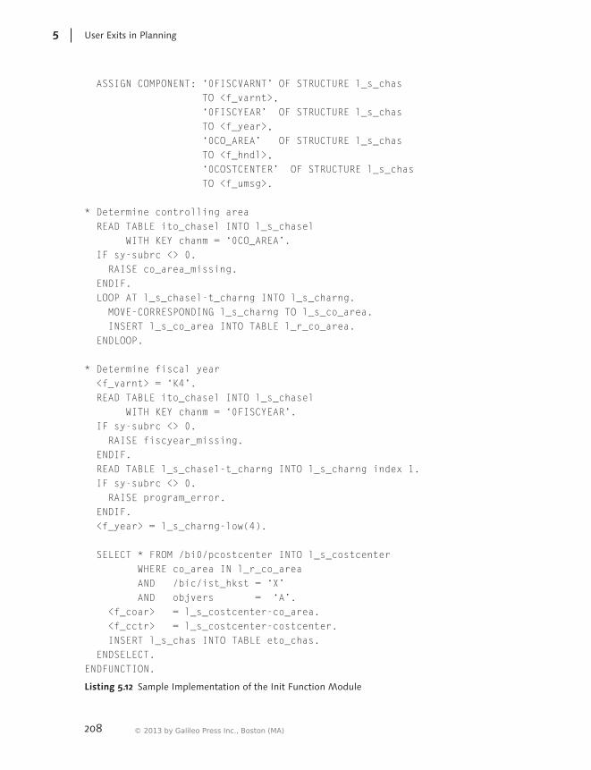
© 2013 by Galileo Press Inc., Boston (MA)208
User Exits in Planning5
ASSIGN COMPONENT: ‘0FISCVARNT’ OF STRUCTURE l_s_chas TO <f_varnt>, ‘0FISCYEAR’ OF STRUCTURE l_s_chas TO <f_year>, ‘0CO_AREA’ OF STRUCTURE l_s_chas TO <f_hndl>, ‘0COSTCENTER’ OF STRUCTURE l_s_chas TO <f_umsg>. * Determine controlling area READ TABLE ito_chasel INTO l_s_chasel WITH KEY chanm = ‘0CO_AREA’. IF sy-subrc <> 0. RAISE co_area_missing. ENDIF. LOOP AT l_s_chasel-t_charng INTO l_s_charng. MOVE-CORRESPONDING l_s_charng TO l_s_co_area. INSERT l_s_co_area INTO TABLE l_r_co_area. ENDLOOP. * Determine fiscal year <f_varnt> = ‘K4’. READ TABLE ito_chasel INTO l_s_chasel WITH KEY chanm = ‘0FISCYEAR’. IF sy-subrc <> 0. RAISE fiscyear_missing. ENDIF. READ TABLE l_s_chasel-t_charng INTO l_s_charng index 1. IF sy-subrc <> 0. RAISE program_error. ENDIF. <f_year> = l_s_charng-low(4). SELECT * FROM /bi0/pcostcenter INTO l_s_costcenter WHERE co_area IN l_r_co_area AND /bic/ist_hkst = ‘X’ AND objvers = ‘A’. <f_coar> = l_s_costcenter-co_area. <f_cctr> = l_s_costcenter-costcenter. INSERT l_s_chas INTO TABLE eto_chas. ENDSELECT. ENDFUNCTION.
Listing 5.12 Sample Implementation of the Init Function Module

209
Exit Functions in Planning 5.3
Example 11: Exit Function Module
The interfaces of the exit function module and the init function module are almost identical. These are the only differences:
EE Table ITO_CHASEL contains a unique value for the characteristic values in the field selection, that is, the value of the characteristic in the current characteristic combination.
EE Table XTH_DATA contains the data of the current characteristic combination. This is a hashed table that contains all characteristics as a key.
The row structure is as follows. Each row of the table contains two structures: S_CHAS and S_KYFS. S_CHAS is the key of the table and comprises all characteris-tics of the planning area, including the units for the key figures. S_KYFS comprises all key figures of the planning area. If new records are created or if existing records are changed, you may fill only those characteristics and key figures that are included in table ITO_CHA or table ITO_KYF; otherwise, you may receive error messages.
EE In the sample function module, table XTH_DATA is typed generically as a hashed table. Then, you must access it using field symbols. If the function module is used in only one planning area, you can also use the generated table type /1SEM/_YTH_DATA_<client><planning area> with row structure /1SEM/_YS_DATA_<client><planning area>. As a result, the function module must contain the records that will be included in the InfoCube for subsequent characteristic combination. SAP BW-BPS then automatically determines the difference from the already existing records.
EE To delete the records, you can either delete the record from table XTH_DATA or set all key figures of the S_KYFS structure to 0. SAP BW-BPS interprets records whose key figures are set to 0 as not existent.
EE New records can be added to the table if the characteristic values correspond to the selections in table ITO_CHASEL.
To get some practice, you should not write the first planning functions generically but specifically to develop a general understanding of how SAP BW-BPS uses this data. The function module shown in Listing 5.13 describes how table XTH_DATA is filled.
FUNCTION Z_KST_IN_TABELLE. *”--------------------------------------------------------- *”*”Local interface: *” IMPORTING

© 2013 by Galileo Press Inc., Boston (MA)210
User Exits in Planning5
*” REFERENCE(I_AREA) TYPE UPC_Y_AREA *” REFERENCE(I_PLEVEL) TYPE UPC_Y_PLEVEL *” REFERENCE(I_METHOD) TYPE UPC_Y_METHOD *” REFERENCE(I_PARAM) TYPE UPC_Y_PARAM *” REFERENCE(I_PACKAGE) TYPE UPC_Y_PACKAGE *” REFERENCE(IT_EXITP) TYPE UPF_YT_EXITP *” REFERENCE(ITO_CHASEL) TYPE UPC_YTO_CHASEL *” REFERENCE(ITO_CHA) TYPE UPC_YTO_CHA *” REFERENCE(ITO_KYF) TYPE UPC_YTO_KYF *” EXPORTING *” REFERENCE(ET_MESG) TYPE UPC_YT_MESG *” CHANGING ** For simplicity reasons, the table is typed because ** it is to be used in planning area DEMOAREA only *” REFERENCE(XTH_DATA) TYPE *” /1SEM/_YTH_DATA_100DEMOAREA *”--------------------------------------------------------- * Field symbol for the row of Table XTH_DATA field-symbols: <s_data> TYPE /1SEM/_YS_DATA_100DEMOAREA. data: l_s_cctr_tab type Z_KST_DATEN, l_s_chasel type upc_ys_chasel, l_s_charng type upc_ys_charng. clear l_s_cctr_tab. * The following assumes that the cost center, the * fiscal year, and the controlling area are * in the field selection. Therefore, they are unique * in the selections. * Determine business year READ TABLE ito_chasel INTO l_s_chasel WITH TABLE KEY chanm = ‘0FISCYEAR’. IF sy-subrc <> 0. RAISE fiscyear_missing. ENDIF. READ TABLE l_s_chasel-t_charng INTO l_s_charng index 1. IF sy-subrc <> 0. RAISE fiscyear_missing. ENDIF. l_s_cctr_tab-FISCYEAR = l_s_charng-low(4). * Determine cost center READ TABLE ito_chasel INTO l_s_chasel WITH TABLE KEY chanm = ‘0COSTCENTER’.

211
Exit Functions in Planning 5.3
IF sy-subrc <> 0. RAISE costcenter_missing. ENDIF. READ TABLE l_s_chasel-t_charng INTO l_s_charng index 1. IF sy-subrc <> 0. RAISE costcenter_missing. ENDIF. l_s_cctr_tab-costcenter = l_s_charng-low(10). * Determine controlling area READ TABLE ito_chasel INTO l_s_chasel WITH TABLE KEY chanm = ‘0CO_AREA’. IF sy-subrc <> 0. RAISE co_area_missing. ENDIF. READ TABLE l_s_chasel-t_charng INTO l_s_charng index 1. IF sy-subrc <> 0. RAISE co_area_missing. ENDIF. l_s_cctr_tab-co_area = l_s_charng-low(4). l_s_cctr_tab-mandt = sy-mandt. * Now, value AMOUNT is determined as the total * of all rows. CLEAR l_s_cctr_tab-amount LOOP AT xth_data assigning <s_data>. CHECK <s_data>-s_kyfs-amount <> 0. ADD <s_data>-s_kyfs-0amount TO l_s_cctr_tab-amount. ENDLOOP. UPDATE Z_KST_DATEN FROM l_s_cctr_tab. * New record? IF sy-subrc <> 0. INSERT Z_KST_DATEN FROM l_s_cctr_tab. ENDIF. ENDFUNCTION.
Listing 5.13 Sample Implementation of the Exit Function Module
5.3.2 Exit Functions in SAP NetWeaver BW Integrated Planning
You can create exit functions in SAP NetWeaver BW Integrated Planning by gener-ating a class that implements one of the interfaces, IF_RSPLFA_SRVTYPE_IMP_EXEC or IF_RSPLFA_SRVTYPE_IMP_EXEC_REF. The first interface is used for functions that
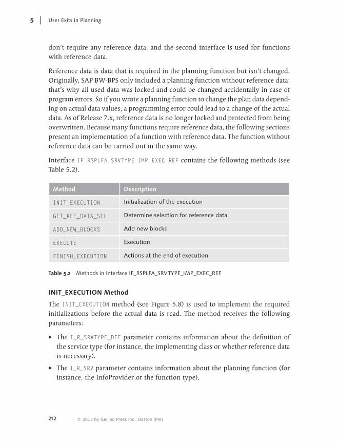
© 2013 by Galileo Press Inc., Boston (MA)212
User Exits in Planning5
don’t require any reference data, and the second interface is used for functions with reference data.
Reference data is data that is required in the planning function but isn’t changed. Originally, SAP BW-BPS only included a planning function without reference data; that’s why all used data was locked and could be changed accidentally in case of program errors. So if you wrote a planning function to change the plan data depend-ing on actual data values, a programming error could lead to a change of the actual data. As of Release 7.x, reference data is no longer locked and protected from being overwritten. Because many functions require reference data, the following sections present an implementation of a function with reference data. The function without reference data can be carried out in the same way.
Interface IF_RSPLFA_SRVTYPE_IMP_EXEC_REF contains the following methods (see Table 5.2).
Method Description
INIT_EXECUTION Initialization of the execution
GET_REF_DATA_SEL Determine selection for reference data
ADD_NEW_BLOCKS Add new blocks
EXECUTE Execution
FINISH_EXECUTION Actions at the end of execution
Table 5.2 Methods in Interface IF_RSPLFA_SRVTYPE_IMP_EXEC_REF
INIT_EXECUTION Method
The INIT_EXECUTION method (see Figure 5.8) is used to implement the required initializations before the actual data is read. The method receives the following parameters:
EE The I_R_SRVTYPE_DEF parameter contains information about the definition of the service type (for instance, the implementing class or whether reference data is necessary).
EE The I_R_SRV parameter contains information about the planning function (for instance, the InfoProvider or the function type).

213
Exit Functions in Planning 5.3
EE The I_R_INFOPROV_DESC parameter contains information about the InfoProvider, for instance, the used characteristics and key figures.
EE The I_R_MSG parameter is used to return messages. For this purpose, you must call the ADD_MSG method of the parameter. This method retrieves its information from the system fields SY-MSGNO, and so on; you don’t have to transfer any parameters.
EE The I_T_DATA_CHARSEL parameter contains the current filters, usually the naviga-tion condition of the query, for which the planning function is called.
Figure 5.8 Signature of the INIT_EXECUTION Method
In most cases, the method remains empty or contains general selections only. A completely generic implementation is very time-consuming.
GET_REF_DATA_SEL Method
The GET_REF_DATA_SEL method is used to determine which data is transferred to the EXECUTE method as reference data. Reference data is data from the InfoProvider that cannot be changed and hence isn’t locked. The signature of the GET_REF_DATA_SEL method is illustrated in Figure 5.9.
Figure 5.9 Signature of the GET_REF_DATA_SEL Method
The I_T_DATA_CHARSEL and I_R_MSG parameters are identical to the INIT_EXECU-TION method. The I_R_PARAM_SET parameter contains the parameters stored in the planning function.
The E_T_REF_CHARSEL and E_TH_NO_REF_BLOCK_DATA return parameters are important:

© 2013 by Galileo Press Inc., Boston (MA)214
User Exits in Planning5
EE E_T_REF_CHARSEL must be filled with selections that are to be valid for the refer-ence data. It usually makes sense to transfer those selections that have been delivered in I_T_DATA_CHARSEL to keep the amount of data to be read low.
EE E_TH_NO_REF_BLOCK_DATA contains characteristics that are to be excluded from the block creation of reference data.
Let’s now further examine the example of Case 3 in Section 5.3.1. If you define the ACTUAL version as reference data and PLAN version as data to be processed, the EXECUTE method is called four times, once for each cost center. The data table and the reference table each contain one record for the cost centers 1000 and 2000, cost center 3000 comprises one record in the reference data but none in the plan data, and cost center 4000 has one record in the plan data but none in the reference data. Usually, this method isn’t called for cost center 4000 because there is no plan data for this cost center. In this example, however, it’s assumed that cost center 4000 is added in method ADD_NEW_BLOCKS, which is described in the following sections.
Let’s assume that no reference data is available, and the average of all cost center actual data is used as the reference date—this constitutes a problem because you receive the records per cost center. Therefore, you have the option to add InfoObject 0COSTCENTER to E_TH_NO_REF_BLOCK_DATA. In this case, the data of all cost centers is transferred to the reference data table.
This method then appears as shown in Listing 5.14.
METHOD IF_RSPLFA_SRVTYPE_IMP_EXEC_REF~GET_REF_DATA_SEL. DATA: s_charsel TYPE RSPLF_S_CHARSEL, s_iobjnm TYPE RSPLF_S_IOBJNM. * Transfer all selections to reference data * except for version LOOP AT i_t_data_charsel INTO s_charsel. IF s_charsel-iobjnm <> ‘0VERSION’. APPEND s_charsel TO e_t_ref_charsel. ENDIF. ENDLOOP. * Add ACTUAL version s_charsel-iobjnm = ‘0VERSION’. s_charsel-sign = ‘I’. s_charsel-opt = ‘EQ’. s_charsel-low = ‘IST’. INSERT s_charsel INTO TABLE e_t_ref_charsel. * Take cost center from block creation

215
Exit Functions in Planning 5.3
s_iobjnm = ‘0COSTCENTER’. INSERT s_iobjnm INTO TABLE e_th_no_ref_block_cha. ENDMETHOD.
Listing 5.14 Sample Implementation of the GET_REF_DATA_SEL Method
ADD_NEW_BLOCKS Method
The ADD_NEW_BLOCKS method (see signature in Figure 5.10) works similar to the init function module of the BW-BPS exit function. It’s used to generate characteristic combinations that don’t appear in the data to be processed (for example, charac-teristic combinations that can only be found in the reference data). This example is frequently used in SAP development for the default copy function of SAP NetWeaver BW Integrated Planning that is implemented in class CL_RSPLFC_COPY.
Figure 5.10 Signature of the ADD_NEW_BLOCKS Method
The ADD_NEW_BLOCKS method contains the known parameters I_R_PARAM_SET and I_R_MSG, as well as the following parameters:
EE I_TH_REF_DATA comprises the reference data with the selections that were deter-mined in the GET_REF_DATA_SEL method.
EE I_TS_EXISTING_BLOCKS contains the combinations that are already included in the plan data. Similar to the SAP BW-BPS function, no combinations can be deleted here.
EE E_TS_NEW_BLOCKS must be filled with additional combinations. If it includes combinations from I_TS_EXISTING_BLOCKS, this is neither a disadvantage nor an advantage.
Listing 5.15 shows the code of the method in class CL_RSPLFC_COPY.
METHOD IF_RSPLFA_SRVTYPE_IMP_EXEC_REF~ADD_NEW_BLOCKS. DATA: l_r_new_block TYPE REF TO data. FIELD-SYMBOLS: <s_ref_data> TYPE ANY, <s_new_block> TYPE ANY.

© 2013 by Galileo Press Inc., Boston (MA)216
User Exits in Planning5
* Generate a new (empty) record CREATE DATA l_r_new_block LIKE LINE OF e_ts_new_blocks. ASSIGN l_r_new_block->* TO <s_new_block>. * Check reference data LOOP AT i_th_ref_data ASSIGNING <s_ref_data>. * Does plan data exist for reference data? MOVE-CORRESPONDING <s_ref_data> TO <s_new_block>. READ TABLE i_ts_existing_blocks TRANSPORTING NO FIELDS FROM <s_new_block>. IF sy-subrc <> 0. * No, insert new combination COLLECT <s_new_block> INTO e_ts_new_blocks. ENDIF. ENDLOOP. ENDMETHOD.
Listing 5.15 Sample Implementation of the ADD_NEW_BLOCKS Method
EXECUTE Method
The EXECUTE method is the central method of the exit function in SAP NetWeaver BW Integrated Planning and must always be implemented. Just as in the SAP BW-BPS exit function, a C_TH_DATA table with the existing plan data is transferred that must then be changed. Figure 5.11 shows the signature of the method.
Figure 5.11 Signature of the EXECUTE Method
The I_R_PARAM_SET, I_TH_REF_DATA, and I_R_MSG parameters are already known; only the I_S_BLOCK_LINE parameter is new. This parameter contains the character-istics that are constant in the current data block.
The example shown in Listing 5.16 copies all values from the reference data of the corresponding cost center to the plan data. If no reference data exists in the cost center, the values of all cost centers are determined.

217
Exit Functions in Planning 5.3
METHOD IF_RSPLFA_SRVTYPE_IMP_EXEC_REF~EXECUTE. FIELD-SYMBOLS: <f_cctr> TYPE /bi0/oicostcenter, <f_cctr_ref> TYPE /bi0/oicostcenter, <f_amount> TYPE /bi0/oiamount, <f_ref_data> TYPE ANY, <f_new_data> TYPE ANY. DATA: l_r_data TYPE REF TO DATA, l_d_amount TYPE /bi0/oiamount, l_d_count TYPE i. * Generate new (empty) record CREATE DATA l_r_data LIKE LINE OF c_th_data. ASSIGN l_r_data->* TO <f_new_data>. * Determine cost center ASSIGN COMPONENT ‘0COSTCENTER’ OF STRUCTURE i_s_block_line TO <f_cctr>. IF sy-subrc <> 0. * Cost center not in block characteristics “Trigger error, wrong configuration ENDIF. * Read reference data for cost center CLEAR l_d_count. LOOP AT i_th_ref_data ASSIGNING <f_ref_data>. ASSIGN COMPONENT ‘0COSTCENTER’ OF STRUCTURE <f_ref_data> TO <f_cctr_ref>. IF <F_CCTR> = <f_cctr_ref>. ADD 1 TO l_d_count. <f_new_data> = <f_ref_data>. REFRESH c_th_data. INSERT <f_new_data> INTO TABLE c_th_data. ENDIF. ENDLOOP. IF l_d_count = 0. * No data found for the corresponding cost center CLEAR l_d_amount. LOOP AT i_th_ref_data ASSIGNING <f_ref_data> . ASSIGN COMPONENT ‘0AMOUNT’ OF STRUCTURE <f_ref_data>

© 2013 by Galileo Press Inc., Boston (MA)218
User Exits in Planning5
TO <f_amount>. IF sy-subrc <> 0. “Trigger error, wrong configuration ENDIF. <f_new_data> = <f_ref_data>. ADD 1 TO l_d_count. ADD <f_amount> TO l_d_amount. ENDLOOP. ASSIGN COMPONENT ‘0AMOUNT’ OF STRUCTURE <f_new_data> TO <f_amount>. IF l_d_count <> 0. <f_amount> = l_d_amount / l_d_count. ELSE. <f_amount> = 0. ENDIF. REFRESH c_th_data. INSERT <f_new_data> INTO TABLE c_th_data. ENDIF. ENDMETHOD.
Listing 5.16 Sample Implementation of the EXECUTE Method
FINISH_EXECUTION Method
The FINISH_EXECUTION method is used to release large internal tables and to carry out similar cleanup tasks. It has one parameter only: I_R_MSG. This parameter is used to return messages (see Figure 5.12). Usually, it should not be implemented because the memory space is often released automatically when the function is completed. Only in the case of large planning sequences may cleansing be neces-sary. You may want to use this method here to write log entries.
Figure 5.12 Signature of the FINISH_EXECUTION Method
5.4 Conclusion
In general, the option to use reference data makes the exit function in SAP NetWeaver BW Integrated Planning considerably more flexible than in SAP BW-BPS. Those of

219
Conclusion 5.4
you who become more familiar with this topic will have the option to write plan-ning functions that would otherwise have resulted in locks within SAP BW-BPS. However, this implementation in SAP NetWeaver BW Integrated Planning sets considerably higher demands on developers because the options of object-oriented programming are used more intensively. You can see this in the object references in the interfaces.
But if you engage with this topic, you can obtain both better ABAP Object know-how and more powerful extension options in SAP NetWeaver BW Integrated Planning. If you cannot get used to it at all, use class CL_RSPLFC_BPS_EXITS, which enables you to create a planning function in SAP NetWeaver BW Integrated Planning that calls function modules of the SAP BW-BPS exit function. However, it’s recommended that you implement the exits anew using an object-oriented approach.

© 2013 by Galileo Press Inc., Boston (MA)
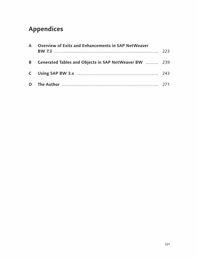
221
Appendices
A Overview of Exits and Enhancements in SAP NetWeaver BW 7.3 ..................................................................................... 223
B Generated Tables and Objects in SAP NetWeaver BW .......... 239
C Using SAP BW 3.x ................................................................... 243
D The Author ............................................................................... 271

© 2013 by Galileo Press Inc., Boston (MA)

223
A Overview of Exits and Enhancements in SAP NetWeaver BW 7.3
The following provides an overview of all helpful BAdIs and exits for working with SAP NetWeaver BW 7.3 as well as other enhancement forms to manipulate the activities of Business Warehouse using ABAP programming. If, during your work, an adaptation option is missing and the appropriate enhancement is not discussed in detail in the enhancement examples in this book, you can use this list as a reference and deploy the corresponding BAdI or exit with the information provided here.
A.1 Enhancements in the Administrator Workbench
This overview starts with the enhancements in the Administrator Workbench. They are particularly important for work with SAP NetWeaver Business Warehouse because the loading of data forms the basis of every activity in SAP NetWeaver BW. For this reason, these enhancements are probably the ones most often implemented in every BW system.
A.1.1 Methods in the Transformation
In the following, you can find all the methods that are used in the transformation.
Start routine
The start routine is called once for each data package at the beginning of the transformation.
Available since: SAP BW 7.0
Call reason: Data extraction via process chains or DTPs in the Administrator Work-bench (Transaction RSA1)
Determining InfoObject values
This method is called for a specific InfoObject of the data target for each data record.

© 2013 by Galileo Press Inc., Boston (MA)224
Overview of Exits and Enhancements in SAP NetWeaver BW 7.3A
Available since: SAP BW 7.0
Call reason: Data extraction via process chains or DTPs in the Administrator Work-bench (Transaction RSA1)
End routine
The end routine is called once for each data package at the end of the transformation.
Available since: SAP BW 7.0
Call reason: Data extraction via process chains or DTPs in the Administrator Work-bench (Transaction RSA1)
Expert routine
The expert routine is called once for each data package instead of the complete transformation.
Available since: SAP BW 7.0
Call reason: Data extraction
A.1.2 Enhancement in Data Transfer Processes
The following enhancement is used in data transfer processes.
Determining filter values
This method is used to determine the filter values in data transfer processes.
Available since: SAP BW 7.0
Call reason: Data extraction
A.1.3 Enhancement in Transfer Rules
The following enhancements are used in transfer rules.

225
Enhancements in the Administrator Workbench A.1
Start routine
The start routine is called once for each data package at the beginning of the trans-fer rules.
Available since: SAP BW 1.x
Call reason: Data extraction via process chains or InfoPackages
Determining InfoObject values
This method is called for a specific InfoObject of the InfoSource for each data record.
Available since: SAP BW 1.x
Call reason: Data extraction via process chains or InfoPackages
A.1.4 Enhancements in Update Rules
The following enhancements play a significant role in update rules.
Start routine
The start routine is called once for each data package at the beginning of the update rules.
Available since: SAP BW 1.x
Call reason: Data extraction via process chains or InfoPackages
Determining InfoObject values
This method is called for a specific InfoObject of the data target for each data record.
Available since: SAP BW 1.x
Call reason: Data extraction via process chains or InfoPackages

© 2013 by Galileo Press Inc., Boston (MA)226
Overview of Exits and Enhancements in SAP NetWeaver BW 7.3A
Determining key figures with unit
This method is called for a specific key figure of the data target for each data record. In contrast to the previous method, a unit is specified in addition to the key figure.
Available since: SAP BW 1.x
Call reason: Data extraction via process chains or InfoPackages
A.1.5 Enhancements in InfoPackages
The following list details only the exits that are essential for working with InfoPackages.
Determining filter values
This exit is used to determine the filter values in InfoPackages.
Available since: SAP BW 1.x
Call reason: Data extraction via process chains or InfoPackages
Determining the file path
This exit is used to determine the file path when files are loaded in SAP NetWeaver BW.
Available since: SAP BW 1.x
Call reason: Data extraction via process chains or InfoPackages
Determining the requests to be deleted
This exit determines the old requests that are to be deleted from the data target after loading.
Available since: SAP BW 1.x
Call reason: Data extraction via process chains or InfoPackages

227
Enhancements in Extraction A.2
A.2 Enhancements in Extraction
The following lists enhancements that are used for data extraction.
A.2.1 User Exits in Function Group XRSA
Initially, you can find the user exits of function group XRSA, that is, the enhance-ments of the extractors in SAP source systems.
Function module EXIT_SAPLRSAP_001
Function module EXIT_SAPLRSAP_001 is used to provide the transaction data extrac-tors with data. Just as in the subsequent modules, you can use it to insert new records, fill new fields, or change delivered field values.
Available since: SAP BW 1.x
Call reason: Extraction of transaction data in the source system
Function module EXIT_SAPLRSAP_002
Function module EXIT_SAPLRSAP_002 is used to provide the master data attribute extractors with data.
Available since: SAP BW 1.x
Call reason: Extraction of master data in the source system
Function module EXIT_SAPLRSAP_003
Function module EXIT_SAPLRSAP_003 is used to provide the master data text extrac-tors with data.
Available since: SAP BW 1.x
Call reason: Extraction of master data in the source system

© 2013 by Galileo Press Inc., Boston (MA)228
Overview of Exits and Enhancements in SAP NetWeaver BW 7.3A
Function module EXIT_SAPLRSAP_004
Function module EXIT_SAPLRSAP_004 is used to provide the hierarchy extractors with data.
Available since: SAP BW 1.x
Call reason: Extraction of hierarchies in the source system
A.2.2 BAdIs in Extraction
Let’s now look at the Business Add-In that is used for extraction.
Business Add-In RSU5_SAPI_BADI
BAdI RSU5_SAPI_BAdI includes methods for enriching extractor data. Enriching texts via BAdIs is not supported here.
Available methods:
EE DATA_TRANSFORM—for enriching transaction data and attributes
EE HIER_TRANSFORM—for enriching hierarchies
Available since: SAP NetWeaver 6.20/SAP BW 3.5
Call reason: Extraction of data in the source system
A.3 Enhancements in Reporting
The following provides an overview of the customer enhancements in reporting.
A.3.1 User Exits in Function Group XRSR
First, you are provided with a list of user exits that are available in function group XRSR. Depending on the function module, they are usually called in reporting for filling variables, reading data, or using the report-report interface.

229
Enhancements in Reporting A.3
Function module EXIT_SAPLRRS0_001
Function module EXIT_SAPLRRS0_001 is used to supply variables in reporting and in authorizations.
Available since: SAP BW 1.x
Call reason: Execution of queries and worksheets
Function module EXIT_SAPLRRS2_001
Function module EXIT_SAPLRRS2_002 is used to calculate characteristic shifts in queries using offset. It is called when you enter an offset for variables in queries, for instance, to specify previous periods.
Available since: SAP BW 1.x
Call reason: Execution of queries and worksheets
Function module EXIT_SAPLRSBBS_001
Function module EXIT_SAPLRSBBS_001 is used to map fields in the report-report interface.
Available since: SAP BW 1.x
Call reason: Navigation from a query to a jump target
Function module EXIT_SAPLRSBBS_002
Function module EXIT_SAPLRSBBS_002 is used to map field names when calling a report in ERP.
Available since: SAP BW 1.x
Call reason: Navigation from a query to a jump target

© 2013 by Galileo Press Inc., Boston (MA)230
Overview of Exits and Enhancements in SAP NetWeaver BW 7.3A
Function module EXIT_SAPMRSRU_001
Function module EXIT_SAPMRSRU_001 is used to define virtual key figures and characteristics.
Available since: SAP BW 1.x
Replaced with BAdI RSR_OLAP_BADI since SAP BW Release 3.5.
Call reason: Execution of queries with virtual InfoObjects
Function module EXIT_SAPMRSRU_999
Function module EXIT_SAPMRSRU_999 is used to initialize the definition of virtual key figures and characteristics.
Available since: SAP BW 1.x
Replaced with BAdI RSR_OLAP_BADI since SAP BW Release 3.5.
Call reason: Execution of queries with virtual InfoObjects
A.3.2 BAdIs in Reporting
The following lists the Business Add-Ins that are deployed in reporting.
BAdI RSR_OLAP_BADI
BAdI RSR_OLAP_BADI is used to calculate virtual key figures and characteristics.
Available methods:
EE DEFINE—to select the characteristics and key figures used
EE INITIALIZE—to initialize the calculation
EE COMPUTE—to run the calculation
Available since: SAP BW 3.x
Call reason: The DEFINE method is called for a query definition; the INITIALIZE method is called once for reading query data, and the COMPUTE method is called once per data record.

231
Enhancements in Reporting A.3
BAdI RSOD_DOC_BADIBAdI RSOD_ITEM_DOCBAdI RSOD_ITEM_DOC_LISTBAdI RSOD_WWW_DOC_MAINT
These BAdIs are used to maintain the documents in reporting, for instance, from the web templates.
Available methods:
EE BAdI RSOD_DOC_BADI:
CHANGE_PROPERTIES
CREATE_PROPERTIES
DELETE_PROPERTIES
HIERARCHY_RESOLVE
SELECT
STORE_CONTENT
EE BAdI RSOD_ITEM_DOC:
CHANGE_RENDERING
EE BAdI RSOD_ITEM_DOC_LIST:
CHANGE_RENDERING
CHANGE_RENDERING_CONTEXT
CHANGE_RENDERING_FUNCTIONS
CHANGE_RENDERING_LIST
EE BAdI RSOD_WW_DOC_MAINT:
BEFORE_RENDERING
DETERMINE_VERSION_HANDLING
Available since: SAP BW 3.x
Call reason: Usage of queries with documents

© 2013 by Galileo Press Inc., Boston (MA)232
Overview of Exits and Enhancements in SAP NetWeaver BW 7.3A
BAdI RS_BBS_BADI
BAdI RS_BBS_BADI is used to calculate own types of jump targets. It is used in very special cases if you want to call own objects from a query, for instance, an external web-based reporting or maintenance application.
Available methods: GET_TYPES
Available since: SAP BW 3.x
Call reason: Execution of queries with jump targets
Enhancement spot RSR_VARIABLE_F4_RESTRICT
Enhancement spot RSR_VARIABLE_F4_RESTRICT is used to restrict the (F4) help in report variables.
These enhancement spots solve a long-known problem in the query execution of InfoObjects with a high number of master data, for instance, in orders. A selec-tion via dimension tables takes a very long time and it delivers too many values.
Available methods:
EE GET_RESTRICTION_FLAT—for the (F4) help of individual values and intervals
EE GET_RESTRICTION_NODE—for the (F4) help of node variables
EE GET_RESTRICTION_HIER—for the (F4) help of hierarchy variables
Available since: SAP NetWeaver BW 7.02
Call reason: Usage of (F4) help for variable selection
A.4 Enhancements in Planning
The planning in SAP NetWeaver BW often does not include exits but only classes and function modules that are copied and adapted. They are listed next.
A.4.1 Enhancements in BW-IP
Enhancements in integrated planning are usually made by implementing own classes that use various predefined interfaces, which you can find in the following.

233
Enhancements in Planning A.4
Interface IF_RSPLS_CR_METHODS
This interface is usually used by entering the superclass CL_RSPLS_CR_EXIT_BASE for a separate class.
Available methods:
EE CHECK—to check characteristic combinations
EE CREATE—to create characteristic combinations
EE DERIVE—to derive characteristic values
Available since: SAP NetWeaver BW 7.0
Call reason: Check and derivation of characteristic value combinations. The corre-sponding class must be entered in the maintenance of characteristic relationships in the planning modeler (Transaction RSPLAN).
Interface IF_RSPLFA_SRVTYPE_IMP_EXEC or IF_RSPLFA_SRVTYPE_IMP_ EXEC_REF
These interfaces are used to create own planning functions. In this context, the IF_RSPLFA_SRVTYPE_IMP_EXEC interface is used to create planning functions without reference data. The IF_RSPLFA_SRVTYPE_IMP_EXEC_REF interface is used to create planning functions with reference data.
Available methods:
EE INIT_EXECUTION—to initiate the planning function
EE GET_REF_DATA_SEL—to specify selections for reference data (only for IF_RSPLFA_SRVTYPE_IMP_EXEC_REF)
EE ADD_NEW_BLOCKS—to create plan values for which the associated characteristic combinations are not yet available in the planning area
EE EXECUTE—to actually execute the planning function
EE FINISH_EXECUTION—for post-processing of planning function
Available since: SAP NetWeaver BW 7.0
Call reason: Self-defined planning function types. The corresponding class must be entered in the maintenance of planning function types (Transaction RSPLAN).

© 2013 by Galileo Press Inc., Boston (MA)234
Overview of Exits and Enhancements in SAP NetWeaver BW 7.3A
Interface IF_RSPLS_DS_EXIT
This interface is used to create own data slices. This way, you can protect specific data against changes, for example, closed periods.
Available methods:
EE IS_PROTECTED—to check whether a characteristic combination is protected from being overwritten
EE IS_OVERLAPPING—to check whether a selection overlaps with the data slice
Available since: SAP NetWeaver BW 7.0
Call reason: Self-defined data slices. The corresponding class must be entered in the maintenance of data slices in the planning modeler (Transaction RSPLAN).
A.4.2 Enhancements in BW-BPS
Enhancements in BW-BPS are usually made by using self-written function modules that use the interfaces of template function modules. These templates are listed here.
Function module UPF_VARIABLE_USER_EXIT
This function module is used as a template for determining variables in BPS. Create a copy and adapt the implementation in this copy.
Available since: SAP BW 3.5
Call reason: BW-BPS variables. The copied function module must be entered for the corresponding variables in the planning area (Transaction BPS0).
Function module UPB_TIME_EXIT_FISC_CHECK
This function module is used as a template for checking characteristic value com-binations in BPS. Create a copy and adapt the implementation in this copy.

235
Additional Enhancements A.5
Available since: SAP BW 3.5
Call reason: BW-BPS characteristic value combinations. The copied function module must be entered for the corresponding characteristic derivation in the planning area (Transaction BPS0).
Function module UPB_TIME_EXIT_FISC_CREATE
This function module is used as a template for checking characteristic value com-binations in BPS. Create a copy and adapt the implementation in this copy.
Available since: SAP BW 3.5
Call reason: BW-BPS characteristic value combinations. The copied function module must be entered for the corresponding characteristic derivation in the planning area (Transaction BPS0).
Function module UPB_TIME_EXIT_FISC_DERIVE
This function module is used as a template for creating characteristic value combi-nations in BPS. Create a copy and adapt the implementation in this copy.
Available since: SAP BW 3.5
Call reason: BW-BPS characteristic value combinations. The copied function module must be entered for the corresponding characteristic derivation in the planning area (Transaction BPS0).
A.5 Additional Enhancements
This section covers BAdIs and enhancement spots that have not been assigned to any of the previous areas but will be helpful in many cases.
BAdI RSAR_CONNECTOR
BAdI RSAR_CONNECTOR is used to calculate customer-specific formulas in the formula editor.

© 2013 by Galileo Press Inc., Boston (MA)236
Overview of Exits and Enhancements in SAP NetWeaver BW 7.3A
Available methods: GET
Available since: SAP BW 3.5
Call reason: Usage of the formula editor in transformations, transfer and update rules, and in selection steps in process chains
BAdI RSRA_ALERT
BAdI RSRA_ALERT is used to export BW alerts for complex controls of processes that are supposed to respond to specific events.
Available methods:
EE INITIALIZE
EE SUBMIT
Available since: SAP BW 3.5
Call reason: Usage of alerts in SAP NetWeaver BW
Enhancement spot RSORA_HINT_EXIT
Enhancement spot RSORA_HINT_EXIT is used to modify hints for the Oracle database. Hints are helps for the Oracle database which can be used to enforce the usage of specific optimized indexes.
Available methods: GET_HINT
Available since: SAP NetWeaver BW 7.0
Call reason: Performance problems in Oracle databases
Enhancement spot RSEC_VIRTUAL_AUTHS
Enhancement spot RSEC_VIRTUAL_AUTHS is used to determine the analysis autho-rizations of a user.
Available methods: GET_AUTHS

237
Additional Enhancements A.5
Available since: SAP NetWeaver BW 7.02
Call reason: Determination of analysis authorizations
BAdI BW_SCHEDULER
BAdI BW_SCHEDULER is used to control subsequent steps after an InfoPackage was executed.
Available methods: USER_EXIT
Available since: SAP BW 3.5
Call reason: Usage of InfoPackages
BAdI OPENHUB_TRANSFORM
BAdI OPENHUB_TRANSFORM is used to transform data if the OpenHub interface is used.
Available methods: TRANSFORM
Available since: SAP BW 3.5
Call reason: Usage of OpenHubs

© 2013 by Galileo Press Inc., Boston (MA)

239
B Generated Tables and Objects in SAP NetWeaver BW
To access data stored in SAP NetWeaver BW and to perform a results check, it’s often very useful to know the data structures contained in the objects. For this reason, the remainder of this appendix lists the most important tables required for the programming process. Although having direct access to the objects is not recommended in all cases, this solution is always available as a last resort.
Note that for all of the following structures, the prefix does not necessarily have to be /BIC/. The prefix of objects from the business content, for instance, is /BI0/, whereas other SAP applications use different namespaces, depending on the application.
B.1 Tables in InfoCubes
Table Name Description
/BIC/F<CUBENAME> Fact table of the InfoCube for noncompressed data records
/BIC/E<CUBENAME> Fact table of the InfoCube for compressed data records
/BIC/D<CUBENAME>X Dimension table of the InfoCube. X is the hexadecimal number for D(imension), P(ackage), U(nit), or T(ime)
/BIC/L<CUBENAME> Data table for inventory values
/BIC/V<CUBENAME>T Structure containing all InfoObjects and navigation attributes
/BIC/V<CUBENAME>F FACTVIEW, a view of the E and F tables. The view can be used for a data mart selection, for example
/BIC/V<CUBENAME>I Structure containing the InfoObjects of the InfoCube
/BIC/V<CUBENAME>N Structure containing the navigation attributes of the InfoCube
/BIC/V<CUBENAME>J Structure containing the InfoObjects of the InfoCube
Table B.1 Tables in InfoCubes

© 2013 by Galileo Press Inc., Boston (MA)240
Generated Tables and Objects in SAP NetWeaver BWB
Table Name Description
/BIC/V<CUBENAME>M Structure containing all InfoObjects and navigation attributes
/BIC/V<CUBENAME>2 Structure containing InfoObjects and navigation attributes, as well as 0INFOPROV and 1ROWCOUNT
/BIC/V<CUBENAME>H Structure containing additional hierarchy surrogate IDs (SIDs)
Table B.1 Tables in InfoCubes (Cont.)
B.2 Tables in DataStore Objects
Table Name Description
/BIC/A<DSNAME>00 Table containing activated data records of the DataStore object
/BIC/A<DSNAME>40 Table containing data records for updating the DataStore object
/BIC/A<DSNAME>50 Table for rolling back the DataStore object
/BIC/0012345678 Table of the change log (corresponds to a PSA table)
Table B.2 Generated Objects of a DataStore Object
B.3 Tables in InfoObjects
Table Name Description
/BIC/P<IOBJNAME> Table containing time-independent master data attributes
/BIC/Q<IOBJNAME> Table containing time-dependent master data attributes
/BIC/S<IOBJNAME> Table containing master data SIDs
/BIC/X<IOBJNAME> Table containing SIDs for time-independent navigation attributes
Table B.3 Tables in InfoObjects

241
Generated Objects in SAP NetWeaver BW B.5
Table Name Description
/BIC/Y<IOBJNAME> Table containing SIDs for time-dependent navigation attributes
/BIC/T<IOBJNAME> Table containing master data texts
/BIC/H<IOBJNAME> Table containing hierarchy nodes and leaves
/BIC/K<IOBJNAME> Table containing SIDs for the hierarchy nodes
/BIC/I<IOBJNAME> Table containing the SID structure
/BIC/J<IOBJNAME> Table of hierarchy intervals
/BIC/OI<IOBJNAME> Data element generated for the InfoObject
/BIC/O<IOBJNAME> Domain generated for the InfoObject
Table B.3 Tables in InfoObjects (Cont.)
B.4 Data Structures in the Data Flow
Structure Name Description
/BIC/0012345678 PSA table
/BIC/CC<XX><DATASRC> Transfer structure
/BIC/CS<INFOSOURCE> Communication structure
Table B.4 Structures in the Data Flow
B.5 Generated Objects in SAP NetWeaver BW
The following objects are database tables generated by SAP NetWeaver BW. They are listed here only for the sake of completeness; you shouldn’t use them in your user exits or BAdIs. However, because basic customer support sometimes seems to have problems with these tables, they are listed here. You can also find information on them in SAP Note 449891.

© 2013 by Galileo Press Inc., Boston (MA)242
Generated Tables and Objects in SAP NetWeaver BWB
Table Name Description
/BI0/01... Intermediate results for query processing
/BI0/02... Intermediate results for external hierarchies that can be reused
/BI0/03... Generated views for query processing
/BI0/04... Stored procedures for compressing InfoCubes
/BI0/05... Trigger for compressing InfoCubes
/BI0/06... Similar to the /BI0/01... tables, but reusable
/BI0/0D... Temporary tables for the open hub
Table B.5 Temporary Tables in SAP NetWeaver BW

243
C Using SAP BW 3.x
SAP BW 3.x doesn’t yet contain any transformations. Instead, it uses transfer rules between DataSource and InfoSource, and update rules between the InfoSource and the data target. Although both types of rules seem to have similar functions—namely, to transform certain data packages into a target structure—there are some differences between them. For example, update rules allow you to create a return table in a routine to make several data records out of one. That’s not possible in a transfer rule. The reason for this can be found in the essentially different require-ments of the two rule types.
C.1 Transfer Rules in SAP BW 3.x
Transfer rules are used essentially to standardize the data that can originate from different source systems. For this purpose, the data records that originate from the source system are usually directly assigned to those records that finally end up in the InfoSource. Routines are needed only to enrich information that isn’t provided or is insufficiently provided in the source system. For this reason, you shouldn’t include fields in the InfoSource that cannot be populated from any of the source systems, unless you definitely have to do so for reasons of compounding.
Of course, there’s an exception to every rule. The most frequent exceptions are constants that are necessary to obtain a data relationship that makes sense. Typical examples of this are the controlling area, the fiscal year variant, and so on. Another example is the use of InfoObjects that are integrated into the InfoSource for use in the transfer rules, either because you want to derive master data attributes from them or because you need the InfoObject for several other routines, and you don’t want to recalculate it every time.
The main purpose of update rules is to format the business data transported in the InfoSource in such a way that an optimal reporting process is enabled for the respective application. In the transfer rules, the target structure is determined by terms that are related to each other regarding business, while the determining fac-tor in the update rules are the reporting demands of the users and hence the data model of the InfoProvider. This means that you can delete the data per your require-ments, split it up, convert it into different units, duplicate records, make several

© 2013 by Galileo Press Inc., Boston (MA)244
Using SAP BW 3.xC
lines out of one, or make one line out of several. All this depends on the reporting requirements and the data model. Usually the data model is denormalized; that is, the data records are complemented with information that is actually redundant, to accelerate the reporting process and enable additional reporting requirements.
Data Model in SAP NetWeaver BW versus Data Model in SAP ERP
The production order (0PRODORDER) contains the plant (0PLANT) in which the order is produced as an attribute. The plant, in turn, contains the country (0COUNTRY) in which the plant is located as an attribute.
In a normal database, you include only the production order in the table. This type of modeling, however, doesn’t allow you to carry out a selection according to the country in SAP NetWeaver BW. For this reason, you include at least the plant, if not the country, in the InfoProvider in SAP NetWeaver BW.
In real life, people usually don’t bother about what they program in the transfer rules and what is programmed in the update rules. Most people aren’t aware of the differences between the two types of rules, and in both routines, the exits are so flexible that nearly all requirements can be handled in both rules. Nevertheless, you should stick to the distinction made here and carry out data-cleaning processes only in the transfer rules, and make adjustments to the contents in the update rules.
The reason for this is simple. If the reporting requirements increase or if new pro-jects require the same data, you may want to add an InfoSource that has already been used to another InfoProvider. But, if you’ve already carried out too many derivations and transformations in the transfer rules, the new InfoProvider will receive the previously transformed data, which may not contain all of the infor-mation required. In the worst case, this may cause the data flow into the original InfoProvider to be completely rewritten, which involves a lot of testing work. That can be avoided by carrying out as few adjustments in the transfer rules as possible.
The transfer rule contains two types of routines: the start routine and the routine needed to derive InfoObject values.
C.1.1 Start Routine in the Transfer Rule
In the transfer rule, you can find the start routine in the Transfer Rules tab above the table that contains the communication structure (see Figure C.1).

245
Transfer Rules in SAP BW 3.x C.1
Figure C.1 Creating a Start Routine
By clicking on the Create or Change button—depending on whether or not a routine already exists—you can navigate to the ABAP Editor that contains the predefined code (see Listing C.1).
PROGRAM CONVERSION_ROUTINE. * Type pools used by conversion program TYPE-POOLS: RS, RSARC, RSARR, SBIWA, RSSM. * Declaration of transfer structure (selected fields only) TYPES: BEGIN OF TRANSFER_STRUCTURE , * InfoObject 0CO_AREA: CHAR - 000004 KOKRS(000004) TYPE C, * InfoObject 0CO_DOC_NO: CHAR - 000010 BELNR(000010) TYPE C, * ... Weitere InfoObjekte ... * InfoObject ZAUTYP: CHAR - 000004 AUART(000004) TYPE C,

© 2013 by Galileo Press Inc., Boston (MA)246
Using SAP BW 3.xC
END OF TRANSFER_STRUCTURE . * Declaration of Data Package TYPES: TAB_TRANSTRU type table of TRANSFER_STRUCTURE. * Global code used by conversion rules *$*$ begin of global – * insert your declaration only below this line *-* * TABLES: ... * DATA: ... *$*$ end of global – * insert your declaration only before this line *-* FORM STARTROUTINE USING G_S_MINFO TYPE RSSM_S_MINFO CHANGING DATAPAK type TAB_TRANSTRU G_T_ERRORLOG TYPE rssm_t_errorlog_int ABORT LIKE SY-SUBRC. “set ABORT <> 0 to “ cancel datapackage *$*$ begin of routine – * insert your code only below this line *-* * DATA: l_s_datapak_line type TRANSFER_STRUCTURE, * l_s_errorlog TYPE rssm_s_errorlog_int. * abort <> 0 means skip whole data package!!! ABORT = 0. *$*$ end of routine – * insert your code only before this line *-* ENDFORM.
Listing C.1 Predefined Code of a Start Routine
The first part of the program code cannot be modified. It informs the developer about the type groups that can be used and, above all, about the transfer structure and the fields it contains.
After that, you can declare global variables. These variables are available not only in the start routine but also in all other routines of the transfer rule. If you want to import and enrich specific data from the database, you should insert a SELECT statement at this point in the start routine to populate an internal table (often a hashed table), which then can be referenced in the individual routines.

247
Transfer Rules in SAP BW 3.x C.1
After that, the actual code of the start routine begins. The start routine contains the USING parameter G_S_MINFO and the CHANGING parameters DATAPAK, G_T_ERRORLOG, and ABORT; the most important parameter is DATAPAK. This parameter is actually a table that contains the transfer structure as data structure as well as all data records of a data package. The start routine isn’t called once per loading process but once per data package. Therefore, you should program a clean code because it’s run through more than once.
The other parameters can be described quickly. The parameter G_S_MINFO has the structure RSSM_S_INFO and contains, among other things, the request number (REQUNO), the data package ID (DATAPAKID), the source system (LOGSYS), the Data-Source (ISOURCE), and some other fields that aren’t used often. The request number and data package ID are rather useful. Using the data package ID, you can ensure that calls which are to be carried out only once, such as writing log entries in cus-tom database tables, are carried out only once.
Logging Data Transfers
For evaluation purposes, you want to log the time at which a data transfer was started. This could be implemented in the start rou tine, as shown in Listing C.2.
FORM STARTROUTINE USING G_S_MINFO TYPE RSSM_S_MINFO CHANGING DATAPAK type TAB_TRANSTRU G_T_ERRORLOG TYPE rssm_t_errorlog_int ABORT LIKE SY-SUBRC. “set ABORT <> 0 to cancel “ data package *$*$ begin of routine – * insert your code only below this line *-* * DATA: l_s_datapak_line type TRANSFER_STRUCTURE, * l_s_errorlog TYPE rssm_s_errorlog_int.* Now follows the assumed structure of * the log table. DATA: begin of l_s_transfer_log, REQUNR TYPE RSREQUNR, DATUM LIKE SY-DATUM, UZEIT LIKE SY-UZEIT, LOGSYS TYPE RSLOGSYS, end of l_s_transfer_log. IF G_S_MINFO-DATAPAKID = 1.

© 2013 by Galileo Press Inc., Boston (MA)248
Using SAP BW 3.xC
* Fill log only once. L_S_TRANSFER_LOG-REQUNR = G_S_MINFO-REQUNR. L_S_TRANSFER_LOG-DATUM = SY-DATUM. L_S_TRANSFER_LOG-UZEIT = SY-UZEIT. L_S_TRANSFER_LOG-LOGSYS = G_S_MINFO-LOGSYS. INSERT L_S_TRANSFER_LOG INTO Z_TRANSFER_LOG. ENDIF. * abort <> 0 means skip whole data package !!! ABORT = 0. *$*$ end of routine – * insert your code only before this line *-* ENDFORM.
Listing C.2 Sample Log Function in the Start Routine
Table G_T_ERRORLOG enables you to return messages that can later be displayed in the monitor. For this purpose, you can create your own messages and message classes via Transaction SE91. Regarding the message return, you should note that the messages can affect the status of the data package. So you should return messages of message type E only if the error is so serious that it would abort the data import process.
In general, you should be economical with your messages. If you comment on every successful record with a corresponding message, the message table will become very large, and this will affect the performance of the import process and of the monitor. Even if the error case is different, you should try to avoid a message.
For example, if during the data-import process, you derive a financial statement item using a routine, and this routine returns an error item in case of an error, you should create a corresponding number of different error items to control the errors rather than output a message in addition to the error item. The message may be ignored in the monitor because the user may think everything is okay because the status of the request is green. The status depends on what percentage of the data is erroneous and how many messages would be generated as a result. Depending on the data quantity, 50 to 100 error messages per import process are certainly acceptable. But if the number is significantly higher, a standard case is made an exception, which unnecessarily increases the error log.
Error Handling in InfoPackages
Appropriate options available for Error handling in the InfoPackage enable you to systematically return error messages and to prevent the InfoPackage from aborting (see Figure C.2).

249
Transfer Rules in SAP BW 3.x C.1
Here you can define the number of permitted errors and the status of the InfoPackage (see Figure C.3). You must make sure that the data package isn’t posted when the number of permitted errors is exceeded. For this reason, if you always want to post data records that don’t contain any errors, you should set a correspondingly high error tolerance. However, this involves the risk of overlooking potential errors or method changes in the source system.
Figure C.2 Calling the Error-Handling Function
Figure C.3 Error-Handling Options
Finally, there’s the ABORT parameter. This parameter aborts the entire data package. This should be used only in absolutely exceptional cases (for example, if required customizing tables haven’t been filled).

© 2013 by Galileo Press Inc., Boston (MA)250
Using SAP BW 3.xC
C.1.2 Routine for InfoObject Derivation
The transfer rules don’t distinguish between routines for characteristics and routines for key figures. Instead, they use a uniform routine that is structured as shown in Listing C.3. To create the routine, you must first click on the InfoObject icon in the left-hand table of the transfer rules (see Figure C.4).
Figure C.4 Button for Creating a Routine
PROGRAM CONVERSION_ROUTINE. * Type pools used by conversion program TYPE-POOLS: RS, RSARC, RSARR, SBIWA, RSSM. * Declaration of transfer structure (selected fields only) TYPES: BEGIN OF TRANSFER_STRUCTURE , * InfoObject 0CO_AREA: CHAR - 000004 KOKRS(000004) TYPE C, * InfoObject 0CO_DOC_NO: CHAR - 000010 * BELNR(000010) TYPE C, * InfoObject 0CO_ITEM_NO: NUMC - 000003 * BUZEI(000003) TYPE N, * InfoObject 0FISCVARNT: CHAR - 000002 * FISCVAR(000002) TYPE C, * ... all fields of the transfer structure ... END OF TRANSFER_STRUCTURE . * Global code used by conversion rules *$*$ begin of global – * insert your declaration only below this line *-* * TABLES: ... * DATA: ... *$*$ end of global – * insert your declaration only before this line *-* *---------------------------------------* * FORM COMPUTE_CO_AREA *---------------------------------------* * Compute value of InfoObject 0CO_AREA * in communication structure * /BI0/CS0CO_OM_OPA_6

251
Transfer Rules in SAP BW 3.x C.1
* Technical properties: * field name = CO_AREA * data element = /BI0/OICO_AREA * data type = CHAR * length = 000004 * decimals = 000000 * ABAP type = C * ABAP length = 000004 * reference field = *---------------------------------------* * Parameters: * --> RECORD_NO Record number * --> TRAN_STRUCTURE Transfer structure * <-- RESULT Return value of InfoObject * <-> G_T_ERRORLOG Error log * <-- RETURNCODE Return code (to skip one record) * <-- ABORT Abort code (to skip whole data * package) *---------------------------------------* FORM COMPUTE_CO_AREA USING RECORD_NO LIKE SY-TABIX TRAN_STRUCTURE TYPE TRANSFER_STRUCTURE G_S_MINFO TYPE RSSM_S_MINFO CHANGING RESULT TYPE /BI0/OICO_AREA G_T_ERRORLOG TYPE rssm_t_errorlog_int RETURNCODE LIKE SY-SUBRC ABORT LIKE SY-SUBRC. “set ABORT <> 0 to cancel “ data package *$*$ begin of routine – * insert your code only below this line *-* * DATA: l_s_errorlog TYPE rssm_s_errorlog_int. RESULT = . * returncode <> 0 means skip this record RETURNCODE = 0. * abort <> 0 means skip whole data package!!! ABORT = 0. *$*$ end of routine – * insert your code only before this line *-* ENDFORM. *---------------------------------------* * FORM INVERT_CO_AREA

© 2013 by Galileo Press Inc., Boston (MA)252
Using SAP BW 3.xC
*---------------------------------------* * Inversion of selection criteria for * InfoObject 0CO_AREA. This subroutine * needs to be implemented only for SAP * RemoteCubes (for better performance) * and for the Report/Report Interface * (drill through). *---------------------------------------* * --> I_RT_CHAVL_CS: Ranges table for * current InfoObject * --> I_THX_SELECTION_CS: Selection * criteria for * all other * InfoObjects * <-- C_T_SELECTION: Selection criteria * for fields of * transfer structure * <-- E_EXACT: Flag Inversion was exact *---------------------------------------* FORM INVERT_CO_AREA USING I_RT_CHAVL_CS TYPE RSARC_RT_CHAVL I_THX_SELECTION_CS TYPE RSARC_THX_SELCS CHANGING C_T_SELECTION TYPE SBIWA_T_SELECT E_EXACT TYPE RS_BOOL. *$*$ begin of inverse routine – * insert your code only below this line *-* DATA: L_S_SELECTION LIKE LINE OF C_T_SELECTION. * An empty selection means all values CLEAR C_T_SELECTION. L_S_SELECTION-FIELDNM = ‘CO_AREA’. * ... * Selection of all values may be not exact E_EXACT = RS_C_FALSE. *$*$ end of inverse routine – * insert your code only before this line *-* ENDFORM.
Listing C.3 Generated Code of the Routine in the Transfer Rule
In the dialog box that displays next, you must select the routine and click on Create (see Figure C.5).

253
Transfer Rules in SAP BW 3.x C.1
Figure C.5 Creating a Routine
Enter a name for the routine and then select those fields of the transfer structure that you want to use in the routine. As shown in Figure C.6, you have the follow-ing options: No field, All Fields, and Selected Fields.
Figure C.6 Selecting the Fields of the Transfer Structure

© 2013 by Galileo Press Inc., Boston (MA)254
Using SAP BW 3.xC
If you need fields from the transfer structure for derivation purposes, you should always select Selected Fields and only select those fields in the table that are required. Selecting the All Fields option may seem to be convenient, but it can affect performance and, in some cases, even result in typos or other errors in the routine going unnoticed until it’s too late. As a matter of fact, it often happens that many InfoObjects with similar names are summarized in one DataSource, and a typo can suddenly cause a different field of the transfer structure to be used. You can avoid this situation by selecting only the required fields from the start.
After you have selected the fields, the code shown in Listing C.3 is displayed. First the transfer structure is defined. This includes only those fields that were selected for use in the routine in the previous step. If you selected No field in the previous step, the transfer structure automatically contains a DUMMY field that is generated only into the structure so that the structure isn’t empty, a situation that would lead to syntax errors. A section for global data follows next. This section is identical to a global section that may be defined in the start routine or in other routines. Changes to it are automatically copied to all other routines of this transfer rule. In particular, you can access internal tables here that were populated in the start routine.
This is followed by the actual routine for determining the return value. This routine contains the following parameters. The TRAN_STRUCTURE parameter contains the fields of the transfer structure that were selected in the previous step exactly as they are delivered from the source system. This parameter is the most important parameter for calculating the values. The most important return parameter is RESULT, which returns the value calculated in the routine. Then there’s the G_T_ERRORLOG table that can be used to return error messages, as well as the two error flags RETURNCODE and ABORT. The value of both flags is 0 if the process did not contain any errors. Their value is different from 0 if either the data record (RETURNCODE) or the entire data package (ABORT) wasn’t processed.
Error Handling in SAP BW 3.x
In SAP BW 3.x, the error-handling process in the transfer rules differs slightly from that in the update rules. The transfer rules comprise a G_T_ERRORLOG table that contains all important information, whereas there are two tables, MONITOR and MONITOR_RECNO in the update rules, whose functions are slightly different. In the start routine, the MONI-TOR table contains only error messages that aren’t associated with a specific row, such as missing customizing tables. The MONITOR_RECNO table, on the other hand, provides the row where the error occurred in addition to the error message itself. However, this requires you to populate the row yourself from the relevant field in the data package.

255
Transfer Rules in SAP BW 3.x C.1
The individual rules of the update rule only contain the MONITOR table, which is com-pleted with the row number after the process.
Table C.1 provides an overview of the table fields in the routines.
Field G_T_ERROR_LOG MONITOR MONITOR_RECNO
Row number Recno Not available Recno
Message class MSGID MSGID MSGID
Message number MSGNO MSGNO MSGNO
Message type MSGTY (I, W, E, A)
MSGTY MSGTY
Message field 1-4 MSGV1 – MSGV4 MSGV1 – MSGV4 MSGV1 – MSGV4
Table C.1 Fields in the Error-Handling Tables
All entries that you insert into the table are displayed in the monitor. Unfortunately, performance decreases with a growing number of messages. You should therefore not use the monitor for debugging purposes or have intermediate results of the calculations output in each line. This can lead to serious performance problems when displaying the results in the monitor, especially when you expand the individual nodes.
You can create new messages in Transaction SE91. The new messages may contain up to four placeholders, which can be included in the message text as &1 through &4.
The routine for calculation is followed by the inversion routine. This routine is almost obsolete today except for RemoteCubes that import data from source systems. In that case, a selection for the characteristic is made up of selections in the query in the source system. For example, if the fields Fiscal Year and Period exist in the source system, and if you restrict the characteristic Fiscal Year/Period in the report to 012.2011 through 001.2012, you use this data to build up the selection 2011 through 2012 for the fiscal year, as data from both 2011 and 2012 is needed. For the period, you must set the selection 001 and 012 because those two periods are contained in the interval. However, this includes more than the original specifica-tion indicated, namely the periods 2011, 012.2011, 001.2012, and 012.2012. For this reason, you would set the E_EXACT parameter to RS_C_FALSE.
C.1.3 Implementing the InfoObject Derivation
As mentioned earlier in this chapter, the transfer rule should mainly be used for data-cleaning purposes. For this reason, there are only a few patterns that are always

© 2013 by Galileo Press Inc., Boston (MA)256
Using SAP BW 3.xC
implemented in the transfer rules in addition to an actual derivation. These patterns predominantly involve the setting of default values.
Setting a Currency
In Listing C.4, different flat files are imported via the same DataSource. Some of the files don’t contain any currency. In this case, you want to use the currency of the controlling area.
*$*$ begin of global – * insert your declaration only below this line *-* * TABLES: ... DATA: g_t_co_area TYPE SORTED TABLE OF /bi0/qco_area WITH UNIQUE KEY CO_AREA OBJVERS DATETO INITIAL SIZE 0, g_w_co_area TYPE /bi0/qco_area. *$*$ end of global – * insert your declaration only before this line *-* FORM COMPUTE_CURRENCY * ... *$*$ begin of routine – * insert your code only below this line *-* * DATA: l_s_errorlog TYPE rssm_s_errorlog_int. DATA: l_d_check_date TYPE d. * Is currency empty? IF TRAN_STRUCTURE-CURRENCY IS INITIAL. * Read controlling areas if that hasn’t been done yet IF LINES( g_t_co_area ) = 0. SELECT * FROM /BI0/QCO_AREA INTO TABLE g_t_co_area. ENDIF. CALL FUNCTION ‘FIRST_DAY_IN_PERIOD_GET’ EXPORTING GJAHR = TRAN_STRUCTURE-fiscyear PERIV = TRAN_STRUCTURE-fiscvarnt POPER = TRAN_STRUCTURE-fiscper3
IMPORTING DATUM = l_d_check_date.
LOOP AT TABLE g_t_co_area INTO g_w_co_area WHERE co_area = TRAN_STRUCTURE-co_area

257
Transfer Rules in SAP BW 3.x C.1
AND objvers = ‘A’ “active master data only AND datefrom <= l_d_check_date AND dateto >= l_d_check_date. * There can only be one valid record in the table, otherwise * the master data of 0CO_AREA is inconsistent. RESULT = g_w_co_area-currency. ENDLOOP. ELSE. * Copy value from file RESULT = TRAN_STRUCTURE-currency. endif. * returncode <> 0 means skip this record RETURNCODE = 0. * abort <> 0 means skip whole data package!!! ABORT = 0. *$*$ end of routine – * insert your code only before this line *-* ENDFORM.
Listing C.4 Sample Implementation of a Characteristics Derivation
The code shown in Listing C.4 is used so often that sometimes it would be useful if the standard attribute derivation could handle this variant. The second variant doesn’t occur as often in everyday life, and it isn’t very convenient either. Often, this variant must be used when a data-loading process aborts for the first time because no attribute could be found for a specific master record. The code is almost identical to the previous example except that the table is read first, and a default value is returned if a record doesn’t exist. Listing C.5 shows a possible excerpt from a corresponding implementation.
*... READ TABLE l_t_posfind INTO l_w_posfind WITH TABLE KEY value_type = TRAN_STRUCTURE-/bic/value_type costelemt = TRAN_STRUCTURE-costelemt. IF SY-SUBRC = 0. RESULT = l_w_posfind-position. ELSE. RESULT = const_default_pos. ENDIF. *...
Listing C.5 Setting a Condition Default Value Example
Because both routines are used often, it’s preferable to have a standard solution available.

© 2013 by Galileo Press Inc., Boston (MA)258
Using SAP BW 3.xC
C.2 Update Rules in SAP BW 3.x
As described in Section C.1, you should use the update rule to format the busi-ness data in such a way that you can generate the required reports. Therefore, you should always bear this aspect in mind during the data-modeling process. Each calculation that you can carry out in the update rules no longer needs to be per-formed at the time of reporting. This way, you can avoid performance problems when running a report.
In contrast to the transfer rules, you cannot simply provide schemas here with regard to what can and cannot be done. The rule of thumb is that everything the user department can describe using an algorithm can actually be implemented. You must consider the following aspects:
EE The algorithms should not require any parameters that the user wants to enter in the report.
EE Particularly with regard to daily processes, it’s significant that the actual data be imported, even if individual entries are missing in control or derivation tables. Nothing is more annoying to the IT department than a loading process that must be checked manually on at least three days out of five.
EE The results should be comprehensible. In complex derivations, all input fields from the data record should therefore be included in the cube. This helps you to analyze errors.
Apart from that, the update rule is the place where you can “make things happen.” Here you can implement the entire logic that is usually handled manually in the user departments, which takes hours and requires hundreds of Excel sheets.
Update Rules
In even older releases—particularly in Release 2.0A, in which the only available data target was the InfoCube—complex implementations of the update rule were handled in a particular way. If, for instance, a file was created each quarter that contained accu-mulated values, but you only wanted to load the delta compared to the last file into the InfoCube, the star schema was read out in the update rules across several selects in the database. In this way, the existing value in the InfoCube was determined for previous periods. This value could then be subtracted from the newly provided value.

259
Update Rules in SAP BW 3.x C.2
This procedure is no longer advisable, and fortunately you can use the DataStore object today to solve such problems more easily. Nevertheless, a lot of things can be learned from this past practice, especially from the recurring surprise that the calculated delta was not correct.
There are some important rules you should consider.
EE When building differences, you must take into account that one key can include sev-eral data records. In this case, you can build the difference only once. For example, if cost center XYZ has two data records—one with the value 100 and one with the value 50—while the InfoCube contains the value 30, you must correct the first value to 70 (= 100 – 30), and leave the second value at 50; that is, you must not correct the second value.
EE This becomes even more complicated if you must maintain a cross-process buffer because the data arrives in several data packages, so you should save the buffer table using the following call:
EXPORT ... TO BUFFER / IMPORT ... FROM BUFFER.
EE If you must access data from other cubes, you should make sure that each cube con-tains two fact tables: the F table (/BIC/F<CUBENAME>) containing the uncompressed requests and the E table (/BIC/E<CUBENAME>) containing the compressed values. However, this procedure isn’t advisable. Section 4.3 described a better way to import content from InfoProviders via VirtualProviders.
Note that selects always affect performance, which is why you should carry out as few selects as possible. In any event, you shouldn’t store the entire contents of a fact table in memory, particularly because you usually don’t notice the resulting memory problems until you carry out the import process in the live system with the relevant data quantities.
In addition, you may regularly come across some usual suspects in the update rules, including complex derivation formulas such as financial statement item determinations, the distribution of data records across several rows, the transfer from the account model to the key figure model and vice versa1, as well as key figure calculations, and aggrega-tions. The problems are always the same—in particular, the problem that when carrying out cross-record calculations, you must take into account that the data records can be contained in different InfoPackages.
The following sections provide useful tricks that help you solve these problems. The update rule contains three different types of routines: the start routine, the routine that determines key figures and data fields, and the routine used to deter-mine the key fields.
1 The difference between the account model and the key figure model is described in detail in SAP Note 407563.

© 2013 by Galileo Press Inc., Boston (MA)260
Using SAP BW 3.xC
C.2.1 Start Routine
The start routine in the update rule is created above the actual update rules (see Figure C.7).
Figure C.7 Calling the Start Routine in the Update Rule
If you open the start routine, a code is generated automatically that is similar to the one shown in Listing C.6.
PROGRAM UPDATE_ROUTINE. *$*$ begin of global – * insert your declaration only below this line *-* * TABLES: ... * DATA: ... *$*$ end of global – * insert your declaration only before this line *-* * The following definition is new in SAP BW 3.x TYPES: BEGIN OF DATA_PACKAGE_STRUCTURE. INCLUDE STRUCTURE /BIC/CS80FIAR_O03. TYPES: RECNO LIKE sy-tabix, END OF DATA_PACKAGE_STRUCTURE. DATA: DATA_PACKAGE TYPE STANDARD TABLE OF DATA_PACKAGE_STRUCTURE

261
Update Rules in SAP BW 3.x C.2
WITH HEADER LINE WITH NON-UNIQUE DEFAULT KEY INITIAL SIZE 0. FORM startup TABLES MONITOR STRUCTURE RSMONITOR “user defined “monitoring MONITOR_RECNO STRUCTURE RSMONITORS “monitoring “with record n DATA_PACKAGE STRUCTURE DATA_PACKAGE USING RECORD_ALL LIKE SY-TABIX SOURCE_SYSTEM LIKE RSUPDSIMULH-LOGSYS CHANGING ABORT LIKE SY-SUBRC. “set ABORT <> 0 to “cancel update *$*$ begin of routine – * insert your code only below this line *-* * fill the internal tables “MONITOR” and/or “MONITOR_RECNO” * to make monitor entries * if abort is not equal zero, the update process will be * canceled ABORT = 0. *$*$ end of routine – * insert your code only before this line *-*
Listing C.6 Generated Code of the Start Routine in the Update Rule
Like the start routine of the transfer rule, the start routine of the update rule begins with a block in which the developer can define global variables. These variables are then made available in all other routines of the update rule. This block is followed by the definition of the data package structure. Here, however, you cannot select the fields you want to transfer because all fields of the InfoSource are transferred.
In addition, each data record contains the corresponding record ID. This ID matches the record ID in the PSA. This means you should always use this record ID instead of a sy-tabix when populating the MONITOR_RECNO table because the data package already may have changed in the transfer rule. The next part of the program code contains the definition of the actual form routine, which is called STARTUP in this example. In the generated program, the routine is called routine_9998. You can view the generated program in the overview screen of the update rule via Extras • Display Activated Program.

© 2013 by Galileo Press Inc., Boston (MA)262
Using SAP BW 3.xC
In addition to the tables MONITOR and MONITOR_RECNO that have already been described in the error-handling note in Section 1.1.4, and the actual data package, DATA_PACK-AGE, the interface only contains the ABORT parameter that aborts the entire data package, and the RECORD_ALL parameter that contains the number of data records.
C.2.2 Filling of Fields in a Data Structure
A typical scenario for applying the start routine is the simultaneous filling of several fields in the data structure. The example shown in Listing C.7 contains an ODS object, COMPONENT, that stores the planned input quantity (PLQUANT) and the actual input quantity (ACTQUANT) for the individual components of production orders. Instead of creating separate routines that read the same data records from one table, you’ll implement the whole process in the start routine. Depending on the application, this can have significant performance benefits, especially if many intermediate results must be calculated in several routines.
FORM startup TABLES MONITOR STRUCTURE RSMONITOR “user defined “monitoring MONITOR_RECNO STRUCTURE RSMONITORS “monitoring “with record n DATA_PACKAGE STRUCTURE DATA_PACKAGE USING RECORD_ALL LIKE SY-TABIX SOURCE_SYSTEM LIKE RSUPDSIMULH-LOGSYS CHANGING ABORT LIKE SY-SUBRC. “set ABORT <> 0 to “cancel update *$*$ begin of routine – * insert your code only below this line *-* * Data package header DATA: l_s_dp_line TYPE data_package_structure. * The comp type contains the structure of the ODS object. types: BEGIN OF comp, plant TYPE /bi0/oiplant, prodorder TYPE /bi0/oiprodorder, component type /bi0/oicomponent, /bic/plquant TYPE /bic/oiplquant, /bic/actquant TYPE /bic/oiactquant, BASE_UOM type /BI0/OIBASE_UOM, END OF comp. * Structures for importing ODS data data: l_s_comp type comp.

263
Update Rules in SAP BW 3.x C.2
statics: l_th_comp type hashed table of comp with unique key plant prodorder component. * Has ODS data been read yet? if l_th_comp[] is INITIAL. * /BIC/ACOMPONENT00is the table with active data of the * ODS component. SELECT * FROM /bic/acomponent00 appending CORRESPONDING FIELDS OF table l_th_comp. endif. * Perform loop across the data package. loop at DATA_PACKAGE INTO l_s_dp_line. * Read components from hashed table read table l_th_comp into l_s_comp with table key plant = l_s_dp_line-plant prodorder = l_s_dp_line-prodorder component = l_s_dp_line-component. if sy-subrc = 0. l_s_dp_line-/BIC/plquant = l_s_comp-/bic/plquant. l_s_dp_line-/bic/actquant = l_s_comp-/bic/actquant. l_s_dp_line-UNIT = l_s_comp-BASE_UOM. * If no record was found, the fields remain empty. * You could also insert an error message into the * MONITOR_RECNO table if the process does not provide * for this. MODIFY DATA_PACKAGE from l_s_dp_line. endif. endloop. * if abort is not equal zero, the update process will be * canceled ABORT = 0. *$*$ end of routine – * insert your code only before this line *-*
Listing C.7 Start Routine Example
C.2.3 Characteristic Calculation
The characteristic calculation in the update rule is essentially identical to the char-acteristic calculation in the transfer rule. The only difference can be found in the parameters. The following sections describe a sample implementation.

© 2013 by Galileo Press Inc., Boston (MA)264
Using SAP BW 3.xC
The problem in the project described here was that specific commitment data could be loaded only once per month in a full upload process. The data could then be assigned to the respective period. However, the aggregation across the different periods produced incorrect results. For this reason, it was decided that after the data was loaded, the value of the last period was to be updated with an inverted mathematical sign into the subsequent period (with the exception of period 12). This way, it became possible to report the various commitment changes in the dif-ferent periods. For this purpose, an additional value type was introduced, and the assignment between the original value type and the delta value type was stored in a database table, Z_VTYPE_CHNG. In controlling, a value type indicates whether the values are planned values, actual values, commitment values, and so on.
The program code in Listing C.8 determines the new value type from the table. If no corresponding entry exists, the record won’t be updated. Moreover, this example deviates from the usual logic because it’s possible for the table to be empty.
FORM compute_key_field TABLES MONITOR STRUCTURE RSMONITOR “user defined “monitoring USING COMM_STRUCTURE LIKE /BIC/CS8DATACUBE RECORD_NO LIKE SY-TABIX RECORD_ALL LIKE SY-TABIX SOURCE_SYSTEM LIKE RSUPDSIMULH-LOGSYS CHANGING RESULT LIKE /BIC/VDATACUBET-VTYPE RETURNCODE LIKE SY-SUBRC ABORT LIKE SY-SUBRC. “set ABORT <> 0 to “cancel update *$*$ begin of routine – * insert your code only below this line *-* * fill the internal table “MONITOR”, to make monitor * entries * ST_VTYPE_CHNG contains the value types to be changed. STATICS : ST_VTYPE_CHNG LIKE SORTED TABLE OF Z_VTYPE_CHNG INITIAL SIZE 0 WITH UNIQUE KEY VTYPE, * SD_DATA_READ is used to check if the data has

265
Update Rules in SAP BW 3.x C.2
* been read. SD_DATA_READ TYPE C VALUE ‘ ’. DATA: LD_VTYPE_CHNG LIKE LINE OF ST_VTYPE_CHNG. * result value of the routine IF SD_DATA_READ IS INITIAL. * No data read, then initialization SELECT * FROM Z_VTYPE_CHNG INTO TABLE ST_VTYPE_CHNG. SD_DATA_READ = ‘X’. ENDIF. READ TABLE ST_VTYPE_CHNG * Does the value type have to be implemented? WITH TABLE KEY VTYPE = COMM_STRUCTURE-VTYPE INTO LD_VTYPE_CHNG . IF SY-SUBRC = 0. * Yes, change value type RESULT = LD_VTYPE_CHNG-VTYPETO. * if the returncode is not equal to 0, the result will not * be updated RETURNCODE = 0. ELSE. * If no entry has been found, then do not update record RETURNCODE = 4. ENDIF. * if abort is not equal zero, the update process will be * canceled ABORT = 0. *$*$ end of routine – * insert your code only before this line *-* ENDFORM.
Listing C.8 Typical Characteristic Derivation in the Update Rule
You can see that, compared to the start routine, the only additional parameters are the record ID RECORD_NO and the return value RESULT. This example contains some typical elements that can usually be found in update rules. For one thing, new characteristic attributes are generated here that don’t occur as such in the source system. For another, data records that won’t be used for reporting are eliminated

© 2013 by Galileo Press Inc., Boston (MA)266
Using SAP BW 3.xC
from the data package. Typically, those two types of elements are implemented in the update rules, not in the transfer rules.
C.2.4 Key Figure Derivation
At best, the key figure or data field derivation in the update rules is almost identi-cal to the characteristic value derivation. The interesting features here are the two checkboxes that are located below the radio button for the creation of a routine (see Figure C.8).
You can use these two checkboxes either to carry out the Unit Calculation in the Routine or—instead of outputting a single key figure—to output a Return Table containing data records.
Figure C.8 Key Figure Calculation in the Update Rule

267
Update Rules in SAP BW 3.x C.2
C.2.5 Unit Calculation
The unit calculation in the routine is required when the DataSource delivers the values in a quantity unit or currency that’s different from the one to be used in the data target. The conversion types in SAP NetWeaver BW are powerful tools for having the system carry out the currency conversion, whereas the conversion of quantity units is practically not supported by SAP NetWeaver BW. For this reason, you should use the unit calculation in the routine for quantity conversions.
Currency Conversion in SAP Systems
Due to legal requirements, the currency conversion function in the various SAP systems is very complex, in particular since the extension caused by the introduction of the euro. For this reason, you should not read the exchange rates from the corresponding TCUR* tables and instead use the conversion types or, if need be, the standard function modules CONVERT_TO_LOCAL_CURRENCY and CONVERT_TO_FOREIGN_CURRENCY.
Listing C.9 shows the determination of the default quantity unit (0BASE_UOM) on the basis of the master data attributes of the material. It then shows the conversion of the delivered quantity unit (0UNIT) into the default quantity unit.
PROGRAM UPDATE_ROUTINE. *$*$ begin of global – * insert your declaration only below this line *-* * TABLES: ... * DATA: ... *$*$ end of global – * insert your declaration only before this line *-* FORM compute_data_field TABLES MONITOR STRUCTURE RSMONITOR “user defined “monitoring USING COMM_STRUCTURE LIKE /BIC/CSABSATZMG RECORD_NO LIKE SY-TABIX RECORD_ALL LIKE SY-TABIX SOURCE_SYSTEM LIKE RSUPDSIMULH-LOGSYS CHANGING RESULT LIKE /BIC/VABSATZT-QUANTITY UNIT LIKE /BIC/VABSATZT-UNIT

© 2013 by Galileo Press Inc., Boston (MA)268
Using SAP BW 3.xC
RETURNCODE LIKE SY-SUBRC ABORT LIKE SY-SUBRC. “set ABORT <> 0 to “cancel update *$*$ begin of routine – * insert your code only below this line *-* * fill the internal table “MONITOR”, to make monitor * entries DATA: l_s_material TYPE /bi0/pmaterial, l_th_material TYPE hashed table OF /bi0/pmaterial WITH UNIQUE KEY material objvers INITIAL SIZE 0, l_d_quantity TYPE /bi0/oiquantity. * result value of the routine IF l_th_material[] IS INITIAL. SELECT * FROM /bi0/pmaterial INTO TABLE l_th_material WHERE objvers = ‘A’. ENDIF. * First determine the basic quantity unit. READ TABLE l_th_material INTO l_s_material WITH TABLE KEY material = COMM_STRUCTURE-material objvers = ‘A’. IF sy-subrc = 0. * Then convert the quantity CALL FUNCTION ‘UNIT_CONVERSION_SIMPLE’ EXPORTING INPUT = COMM_STRUCTURE-quantity UNIT_IN = COMM_STRUCTURE-unit UNIT_OUT = l_s_material-base_uom EXPORTING OUTPUT = l_d_quantity EXCEPTIONS OTHERS = 1 . IF sy-subrc = 0. * Conversion successful RESULT = l_d_quantity. UNIT = l_s_material-base_uom.

269
Update Rules in SAP BW 3.x C.2
ELSE. * If conversion not possible, copy original values RESULT = COMM_STRUCTURE-quantity. UNIT = COMM_STRUCTURE-unit. ENDIF. ELSE. * If no basic quantity unit available, copy * quantity and unit RESULT = COMM_STRUCTURE-quantity. UNIT = COMM_STRUCTURE-unit. ENDIF. * if the returncode is not equal zero, the result will not * be updated RETURNCODE = 0. * if abort is not equal zero, the update process will be * canceled ABORT = 0. *$*$ end of routine – * insert your code only before this line *-* ENDFORM.
Listing C.9 Sample Unit Conversion
The example has been programmed as very error-tolerant, in that it ignores all errors, be they missing master data or incompatible quantity units. This leads back to the fact that the original values are written to the InfoCube. This procedure is often used, particularly if it’s clear that, because of the nature of the business process, no data consistency can be guaranteed. If the quantity data is used only for reporting purposes and not as input data for other algorithms such as cost dis-tributions, a consistent supply of units is no longer required. And if the processes are redesigned in such a way that the source system provides only quantity units that can be converted, and the master data is available on time, the data quality in SAP NetWeaver BW is improved.
In practice, you should always output error messages during the test phase to evaluate data quality. In a live system, you only extend those error messages if you find out that almost every loading process contains erroneous data. Otherwise, you should at least output information messages (I messages).

© 2013 by Galileo Press Inc., Boston (MA)270
Using SAP BW 3.xC
If the information is needed consistently in subsequent steps or downstream sys-tems, the update process in the InfoProvider must be stopped here. You can do that by setting the RETURNCODE to 4.
C.2.6 Return Table
The return table differs from all other routines in that it’s the only routine that allows you to return the data records in the data-target structure. Note, however, that you must make sure to use only the key figure or data field for which the routine was actually created.
This option is particularly interesting if you want to calculate the entire result to be written into the InfoCube in the start routine and store this result in the global data. In the return table, you then can copy the global data in Record 1, while the data remains empty for all other records. In this way, you can directly calculate the cube results.
The routine that’s now generated contains the familiar parameters MONITOR, COMM_STRUCTURE, RECORD_NO, RECORD_ALL, SOURCE_SYSTEM, RETURNCODE, and ABORT. Addi-tionally, it contains two new parameters: the RESULT_TABLE table, which replaces the return value RESULT, and the structure ICUBE_VALUES, which contains the results of the data field derivations. This demonstrates the logic SAP BW 3.x uses to calculate the update rules. First it calculates the characteristic values and then the key figure. However, when in doubt, it’s safer to rely on the communication structure and build up the entire table from there.

271
D The Author
After graduating with a degree in business mathematics from Technische Universität Berlin, Germany, Dirk Herzog started his career in 1996 in the CO-OM development department at SAP in Walldorf, Germany. His work focused on cost center planning and the CO planning processor.
Four years later, he moved back to Berlin to join the BW consulting team at SAP Deutschland. Since then, he has led
numerous national and international implementations of SAP NetWeaver Business Warehouse and SAP Strategic Enterprise Management. These have included the world’s first SAP BW 3.0 project, one of the first cube-based SEM-BCS implementa-tions, and a large business plan for the German sales division of a large automotive manufacturer.
Dirk also has developed solutions and solution concepts for complex modeling and implementation. He is co-author of the PDEBWB course on “User Exits in SAP BW” and has taught the course several times. When he’s not spending time with his two children, Dirk blogs in the SAP Community Network (SCN) and answers questions.

© 2013 by Galileo Press Inc., Boston (MA)
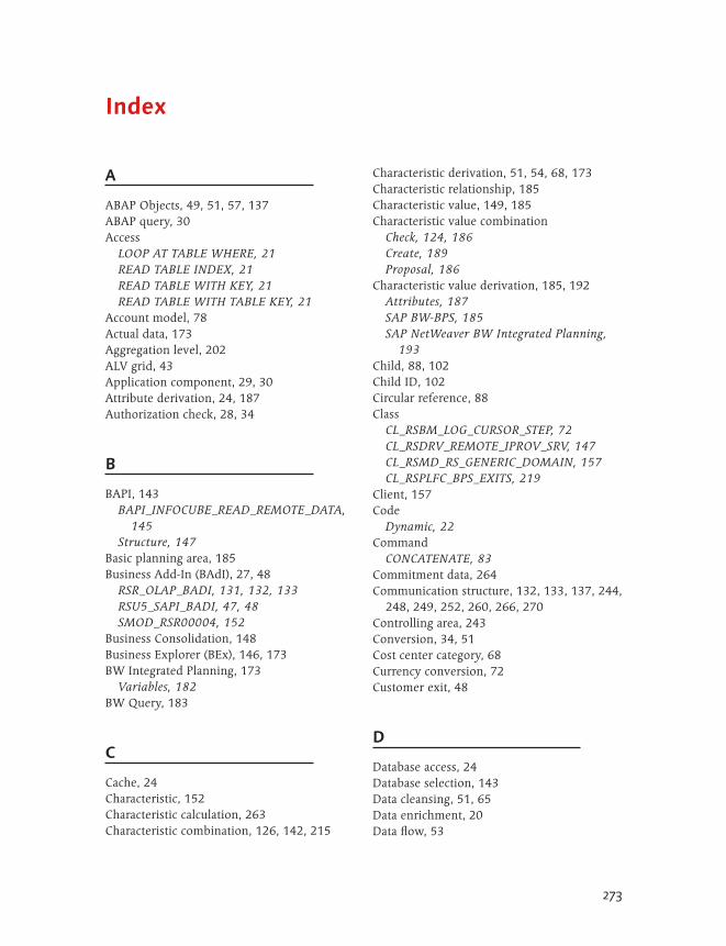
273
A
ABAP Objects, 49, 51, 57, 137ABAP query, 30Access
LOOP AT TABLE WHERE, 21READ TABLE INDEX, 21READ TABLE WITH KEY, 21READ TABLE WITH TABLE KEY, 21
Account model, 78Actual data, 173Aggregation level, 202ALV grid, 43Application component, 29, 30Attribute derivation, 24, 187Authorization check, 28, 34
B
BAPI, 143BAPI_INFOCUBE_READ_REMOTE_DATA,
145Structure, 147
Basic planning area, 185Business Add-In (BAdI), 27, 48
RSR_OLAP_BADI, 131, 132, 133RSU5_SAPI_BADI, 47, 48SMOD_RSR00004, 152
Business Consolidation, 148Business Explorer (BEx), 146, 173BW Integrated Planning, 173
Variables, 182BW Query, 183
C
Cache, 24Characteristic, 152Characteristic calculation, 263Characteristic combination, 126, 142, 215
Characteristic derivation, 51, 54, 68, 173Characteristic relationship, 185Characteristic value, 149, 185Characteristic value combination
Check, 124, 186Create, 189Proposal, 186
Characteristic value derivation, 185, 192Attributes, 187SAP BW-BPS, 185SAP NetWeaver BW Integrated Planning,
193Child, 88, 102Child ID, 102Circular reference, 88Class
CL_RSBM_LOG_CURSOR_STEP, 72CL_RSDRV_REMOTE_IPROV_SRV, 147CL_RSMD_RS_GENERIC_DOMAIN, 157CL_RSPLFC_BPS_EXITS, 219
Client, 157Code
Dynamic, 22Command
CONCATENATE, 83Commitment data, 264Communication structure, 132, 133, 137, 244,
248, 249, 252, 260, 266, 270Controlling area, 243Conversion, 34, 51Cost center category, 68Currency conversion, 72Customer exit, 48
D
Database access, 24Database selection, 143Data cleansing, 51, 65Data enrichment, 20Data flow, 53
Index

© 2013 by Galileo Press Inc., Boston (MA)274
Index
Data modeling, 43, 78, 243, 258Data owner, 34Data package, 25, 32, 33, 36, 53, 247, 249,
262Data quality, 269Data record, 17
Sequence, 141Data selection, 146DataSource, 28, 35, 47, 48, 51, 68, 89, 90,
143, 149, 243Create, 90Export, 45Generic, 28, 31
DataStore, 39, 149Object, 88, 91, 109, 142
Data target, 78, 243Structure, 270Update, 25
Data transfer process (DTP), 81, 88, 103, 105Characteristics value selection, 83Selection of a file name, 81
Data volume, 17Default value, 128, 256
Date-dependent, 114Table-dependent, 114
Deleting redundant records, 65Delta
Generic, 32Upload, 32
Distribution mechanism, 48
E
Elimination of intercompany sales, 142End routine, 53, 63, 68, 72, 88, 94, 101, 105Enterprise data warehouse, 53Error handling, 72, 262
SAP BW 3.x, 254Error message, 126, 248
Output, 269Return, 128
ExceptionINVALID, 187
Exit functionSAP BW-BPS, 203
Exit function (Cont.)SAP NetWeaver BW Integrated Planning,
211Exit function module, 206, 209Expert routine, 63, 69, 71, 72, 78, 80Extraction, 27, 48
SAP ERP, 40Extractor, 36
Add data records, 39Checker, 33Generic, 27, 28, 32, 33, 45
Extract structure, 46Fill, 38
F
FieldChange, 205Extension, 33FIELDNAME, 85I_S_RKB1D-COMPID, 128Masking, 28
Field symbol, 17, 22File name
Determine, 82Selection, 81
Filter value, 109Determination, 86
Fiscal year variant, 157, 243Flat files, 28Full table scan, 21Full upload, 32Function
CREATE, 192WS_UPLOAD, 203
Function module, 35BAPI_INFOCUBE_READ_REMOTE_DATA,
145, 146Calculate data, 143CONVERT_TO_FOREIGN_CURRENCY, 267CONVERT_TO_LOCAL_CURRENCY, 267Exit function module, 206, 209EXIT_SAPLRRS0_001, 107EXIT_SAPLRSAP_001, 35, 37EXIT_SAPLRSAP_002, 35EXIT_SAPLRSAP_003, 35

275
Index
Function module (Cont.)EXIT_SAPLRSAP_004, 35, 45EXIT_SAPLRSR0_001, 109Fixed interface, 175Init function module, 206RRMS_MESSAGE_HANDLING, 128, 129RSDRI_INFOPROV_READ, 149Z_VAR_CHECK_VALIDITY, 113, 124
G
GroupSemantic, 103
H
Hierarchy, 28, 35, 43, 47, 86, 187Aggregation, 142BW hierarchy, 87Exit, 45Extractor, 45Sorted, 87
I
I message, 269Implementation logic, 56Implementation name, 133Import process, 57Include
ZXRSAU01, 36ZXRSRU01, 107
Index, 102Individual processing, 141InfoCube, 65, 72, 142, 145, 149, 152, 205,
269, 270InfoObject, 39, 102, 130, 172, 192, 214
0AMOUNT, 780BUS_AREA, 1150COMPANY, 1150CURRENCY, 630QUANTITY, 78BASE_CCT, 171Derivation, 250, 255
InfoPackage, 83, 103, 109, 249, 259InfoProvider, 51, 71, 130, 131, 142, 143, 144,
152, 156, 173, 243, 244InfoSource, 53, 71, 243, 244, 261Initialization, 65Instance attribute, 137
K
Key, 88Key field, 18
ITO_KYF, 206KEYDATE, 145
Key figure, 149, 152Calculation, 61Derivation, 58, 266Model, 78Virtual, 130
L
Line items report, 78Link node, 102Loading process, 17Log, 80Loop, 20
M
Mapping, 152, 153Masking, 33Master data attribute, 19, 35Master data read class, 172
Create, 157Implementation, 164
Master data read routine, 156Master data table, 149Master data text, 35Message, 248Message class, 248Message collector, 128Method
ADD_NEW_BLOCKS, 215COMPUTE, 134, 137, 138, 139, 140, 141

© 2013 by Galileo Press Inc., Boston (MA)276
Index
Method (Cont.)CONSTRUCTOR, 141CREATE, 158DATA_TRANSFORM, 47DEFINE, 134, 136, 137EXECUTE, 216EXIT_SAPLRSBBS_001, 153EXIT_SAPLRSBBS_002, 153EXPERT_ROUTINE, 77FINISH_EXECUTION, 218GET_ATTRIBUTES, 163, 168GET_CAPABILITIES, 159GET_REF_DATA_SEL, 213GET_TEXT, 163, 170GET_VALUES, 160, 166HIER_TRANSFORM, 47, 48IF_RSPLS_CR_METHODS~CHECK, 194IF_RSPLS_CR_METHODS~CREATE, 197IF_RSPLS_CR_METHODS~DERIVE, 201INIT_EXECUTION, 212INITIALIZATION, 134, 137, 138INVERSE_EXPERT_ROUTINE, 77INVERSE_EXPERT_SELECTION, 77SET_KEY_DATE, 159_VALUES_GENERATE, 164, 168
Microsoft Excel, 86Table, 86
Multi-planning area, 185MultiProvider, 130, 143, 152
N
Navigation attribute, 146, 172Navigation block, 109Next ID, 102Node, 87, 102
Node ID, 87Root node, 87
O
Object reference, 219ODS object, 88
OLAP processor, 147O notation, 22Original object, 28
P
ParameterI_IOBJNM, 110I_MAXROWS, 161I_PERIV, 111I_S_COB_PRO, 110I_S_RKB1D, 110I_STEP, 108, 111, 113, 118, 121, 123I_T_VAR_RANGE, 111I_VARTYP, 110I_VNAM, 110
Parent, 102Parent ID, 102Performance, 17, 18, 22, 72, 77, 130, 143,
254, 255, 258, 259Per data record, 17
Period entry, 126Persistent staging area (PSA), 25, 81, 261Planning function, 173, 178, 204, 209Planning level, 175, 185Plan version, 175Position selection, 68Pre-assignment, 178
Based on authorizations, 115Program
Activated, 261
Q
Quantity unitConversion, 61
Quarterly report, 125Query, 105, 149Query creation, 182Query Designer, 121Query name, 156

277
Index
R
Read accessTable, 20
Read table entry, 141Reference data, 212, 214, 216RemoteCube, 143, 255Report-report interface, 77, 152, 153Return table, 243, 270Return value set, 177, 179RFC Packing, 144, 147, 148Rounding difference, 143Routine
Create, 82Unit, 59
S
SAP BW-BPS, 173Variables, 174, 182
SAP ERP, 173SAP NetWeaver 7.0, 51SAP NetWeaver 7.3, 52SAP NetWeaver BW 7.0, 51, 71, 86, 88, 90,
103, 105SAP NetWeaver BW 7.3, 64, 106SAP SEM-BCS, 148Selection column, 32Selection condition, 202Selection field, 32, 46Selection option variable, 183SID Support, 144, 147, 148Single value, 177
Return, 175Source characteristic, 192Source structure, 80Source system, 28, 77, 78, 243, 254, 255Special character
Removal, 57Standard deviation, 141Standard extractor, 27, 33
Enhancement, 28Start routine, 53, 63, 67, 68, 72, 88, 105, 244,
246, 254, 260, 261, 270
StatementCASE, 37CX_RSROUT_ABORT, 57CX_RSROUT_SKIP_RECORD, 57RAISE EXCEPTION, 128SELECTION, 146
T
Table, 29ANY TABLE, 38CHARACTERISTICS, 146C_T_DATA, 38C_T_FOLDERT, 44C_TH_DATA, 216C_T_HIENODE, 44C_T_MESSAGES, 38Customizing table, 249DATA, 147Error handling, 255ET_MESG, 206ETO_CHAS, 206E_T_RANGE, 111G_T_ERRORLOG, 254Hashed table, 19, 21, 24, 246IT_EXITP, 206ITO_CHA, 206ITO_CHASEL, 206, 209ITO_KYF, 206I_T_SELOPT, 161I_TS_REQ_ATR, 161KEYFIGURES, 146L_T_RANGE, 85Mapping table, 39MONITOR_RECNO, 261RANGES, 179RESULT_PACKAGE, 76RESULT_TABLE, 270Sorted table, 18, 21SOURCE_PACKAGE, 65Standard table, 18, 21S_T_TCURF, 42TCURR, 29, 31, 42XTH_DATA, 209

© 2013 by Galileo Press Inc., Boston (MA)278
Index
Table access, 21Table definition, 20Table type, 17, 18Target structure, 80Transaction
BPS0, 174CMOD (Maintainance of SAP Extensions),
34LISTCUBE, 152RSA3, 33RSBBS, 153RSO2 (Create Generic Extractor), 28RSRT, 78SBIW (Edit Application Component
Hierarchy), 30SE19, 132SE80, 157, 164, 194SE91, 129, 248, 255
Transaction data, 29, 35Transfer rule, 51, 105, 243, 244, 246, 254
Start routine, 33Transfer structure, 247, 254Transformation, 51, 53, 63, 68, 86
Graphical display, 52History, 72
Transport, 72Type
_ty_s_SC_1, 56_ty_s_TG_1, 56
U
Unit calculation, 58, 267Unit output, 61Update rule, 24, 51, 63, 105, 243, 244, 254,
258, 260, 261, 263, 266, 267, 270Upload, 19Usage type, 27User exit, 27, 34, 43, 46
EXIT_SAPLRRS0_001, 139, 142
User exit (Cont.)EXIT_SAPLRSAP_001, 36Planning, 173RSAP0001, 33, 34, 47RSR00001, 107RSR00002, 131RSR00004, 152
V
Validation, 108, 124, 125Variable, 107, 173
Central, 124Check, 123Combination, 124Derivation, 121Handling, 123Planning, 173Project-specific, 124Read, 182Set, 174Strategy, 124Transfer, 142, 183Value, 142Write, 184
Variable determinationExample, 121
Variable exit, 107, 174ZXRSRU01, 113
Variation, 141Views, 29Virtual characteristic, 130VirtualProvider, 77, 143, 144, 149, 152
Implementation, 148
X
X message, 145


Service Pages
The following sections contain notes on how you can contact us.
Praise and Criticism
We hope that you enjoyed reading this book. If it met your expectations, please do recommend it, for example, by writing a review on http://www.sap-press.com. If you think there is room for improvement, please get in touch with the editor of the book: [email protected]. We welcome every suggestion for improvement but, of course, also any praise!
You can also navigate to our web catalog page for this book to submit feedback or share your reading experience via Facebook, Google+, Twitter, email, or by writing a book review. Simply follow this link: http://www.sap-press.com/H3257.
Supplements
Supplements (sample code, exercise materials, lists, and so on) are provided in your online library and on the web catalog page for this book. You can directly navigate to this page using the following link: http://www.sap-press.com/H3257. Should we learn about typos that alter the meaning or content errors, we will provide a list with corrections there, too.
Technical Issues
If you experience technical issues with your e-book or e-book account at SAP PRESS, please feel free to contact our reader service: [email protected].
i

ii
About Us and Our Program
The website http://www.sap-press.com provides detailed and first-hand information on our current publishing program. Here, you can also easily order all of our books and e-books. For information on Galileo Press Inc. and for additional contact options please refer to our company website: http://www.galileo-press.com.

iii
Legal Notes
This section contains the detailed and legally binding usage conditions for this e-book.
Copyright Note
This publication is protected by copyright in its entirety. All usage and exploitation rights are reserved by the author and Galileo Press; in particular the right of repro-duction and the right of distribution, be it in printed or electronic form.
© 2012 by Galileo Press Inc., Boston (MA)
Your Rights as a User
You are entitled to use this e-book for personal purposes only. In particular, you may print the e-book for personal use or copy it as long as you store this copy on a device that is solely and personally used by yourself. You are not entitled to any other usage or exploitation.
In particular, it is not permitted to forward electronic or printed copies to third parties. Furthermore, it is not permitted to distribute the e-book on the Internet, in intranets, or in any other way or make it available to third parties. Any public exhibition, other publication, or any reproduction of the e-book beyond personal use are expressly prohibited. The aforementioned does not only apply to the e-book in its entirety but also to parts thereof (e.g., charts, pictures, tables, sections of text).
Copyright notes, brands, and other legal reservations as well as the digital watermark may not be removed from the e-book.
Digital Watermark
This e-book copy contains a digital watermark, a signature that indicates which person may use this copy. If you, dear reader, are not this person, you are violating the copyright. So please refrain from using this e-book and inform us about this violation. A brief email to [email protected] is sufficient. Thank you!

iv
Trademarks
The common names, trade names, descriptions of goods, and so on used in this publication may be trademarks without special identification and subject to legal regulations as such.
All of the screenshots and graphics reproduced in this book are subject to copyright © SAP AG, Dietmar-Hopp-Allee 16, 69190 Walldorf, Germany. SAP, the SAP logo, mySAP, mySAP.com, SAP Business Suite, SAP NetWeaver, SAP R/3, SAP R/2, SAP B2B, SAPtronic, SAPscript, SAP BW, SAP CRM, SAP EarlyWatch, SAP ArchiveLink, SAP HANA, SAP GUI, SAP Business Workflow, SAP Business Engineer, SAP Business Navigator, SAP Business Framework, SAP Business Information Warehouse, SAP interenterprise solutions, SAP APO, AcceleratedSAP, InterSAP, SAPoffice, SAPfind, SAPfile, SAPtime, SAPmail, SAP-access, SAP-EDI, R/3 Retail, Accelerated HR, Acceler-ated HiTech, Accelerated Consumer Products, ABAP, ABAP/4, ALE/WEB, Alloy, BAPI, Business Framework, BW Explorer, Duet, Enjoy-SAP, mySAP.com e-business platform, mySAP Enterprise Portals, RIVA, SAPPHIRE, TeamSAP, Webflow, and SAP PRESS are registered or unregistered trademarks of SAP AG, Walldorf, Germany.
Limitation of Liability
Regardless of the care that has been taken in creating texts, figures, and programs, neither the publisher nor the author, editor, or translator assume any legal respon-sibility or any liability for possible errors and their consequences.