sample-level deep convolutional neural networks for music ... · sample-level deep convolutional...

SAMPLE-LEVEL DEEP CONVOLUTIONAL NEURAL NETWORKS FORMUSIC AUTO-TAGGING USING RAW WAVEFORMS

Jongpil Lee Jiyoung Park Keunhyoung Luke Kim Juhan NamKorea Advanced Institute of Science and Technology (KAIST)

[richter, jypark527, dilu, juhannam]@kaist.ac.kr

ABSTRACT

Recently, the end-to-end approach that learns hierarchi-cal representations from raw data using deep convolutionalneural networks has been successfully explored in the im-age, text and speech domains. This approach was appliedto musical signals as well but has been not fully exploredyet. To this end, we propose sample-level deep convolu-tional neural networks which learn representations fromvery small grains of waveforms (e.g. 2 or 3 samples) be-yond typical frame-level input representations. Our exper-iments show how deep architectures with sample-level fil-ters improve the accuracy in music auto-tagging and theyprovide results comparable to previous state-of-the-art per-formances for the Magnatagatune dataset and Million SongDataset. In addition, we visualize filters learned in a sample-level DCNN in each layer to identify hierarchically learnedfeatures and show that they are sensitive to log-scaled fre-quency along layer, such as mel-frequency spectrogramthat is widely used in music classification systems.

1. INTRODUCTION

In music information retrieval (MIR) tasks, raw waveformsof music signals are generally converted to a time-frequencyrepresentation and used as input to the system. The ma-jority of MIR systems use a log-scaled representation infrequency such as mel-spectrograms and constant-Q trans-forms and then compress the amplitude with a log scale.The time-frequency representations are often transformedfurther into more compact forms of audio features depend-ing on the task. All of these processes are designed basedon acoustic knowledge or engineering efforts.

Recent advances in deep learning, especially the devel-opment of deep convolutional neural networks (DCNN),made it possible to learn the entire hierarchical represen-tations from the raw input data, thereby minimizing theinput data processing by hands. This end-to-end hierar-chical learning was attempted early in the image domain,particularly since the DCNN achieves break-through re-sults in image classification [1]. These days, the method ofstacking small filters (e.g. 3x3) is widely used after it hasbeen found to be effective in learning more complex hier-archical filters while conserving receptive fields [2]. In the

Copyright: c© 2017 Jongpil Lee et al. This is an open-access article distributed

under the terms of the Creative Commons Attribution 3.0 Unported License, which

permits unrestricted use, distribution, and reproduction in any medium, provided

the original author and source are credited.

text domain, the language model typically consists of twosteps: word embedding and word-level learning. Whileword embedding plays a very important role in languageprocessing [3], it has limitations in that it is learned inde-pendently from the system. Recent work using CNNs thattake character-level text as input showed that the end-to-end learning approach can yield comparable results to theword-level learning system [4, 5]. In the audio domain,learning from raw audio has been explored mainly in theautomatic speech recognition task [6–10]. They reportedthat the performance can be similar to or even superior tothat of the models using spectral-based features as input.

This end-to-end learning approach has been applied tomusic classification tasks as well [11, 12]. In particular,Dieleman and Schrauwen used raw waveforms as input ofCNN models for music auto-tagging task and attempted toachieve comparable results to those using mel-spectrogramsas input [11]. Unfortunately, they failed to do so and at-tributed the result to three reasons. First, their CNN mod-els were not sufficiently expressive (e.g. a small number oflayers and filters) to learn the complex structure of poly-phonic music. Second, they could not find an appropriatenon-linearity function that can replace the log-based am-plitude compression in the spectrogram. Third, the bottomlayer in the networks takes raw waveforms in frame-levelwhich are typically several hundred samples long. Thefilters in the bottom layer should learn all possible phasevariations of periodic waveforms which are likely to beprevalent in musical signals. The phase variations within aframe (i.e. time shift of periodic waveforms) are actuallyremoved in the spectrogram.

In this paper, we address these issues with sample-levelDCNN. What we mean by “sample-level” is that the fil-ter size in the bottom layer may go down to several sam-ples long. We assume that this small granularity is anal-ogous to pixel-level in image or character-level in text.We show the effectiveness of the sample-level DCNN inmusic auto-tagging task by decreasing strides of the firstconvolutional layer from frame-level to sample-level andaccordingly increasing the depth of layers. Our exper-iments show that the depth of architecture with sample-level filters is proportional to the accuracy and also the ar-chitecture achieves results comparable to previous state-of-the-art performances for the MagnaTagATune dataset andthe Million Song Dataset. In addition, we visualize filterslearned in the sample-level DCNN.

arX

iv:1

703.

0178

9v2

[cs

.SD

] 2

2 M

ay 2

017

http://creativecommons.org/licenses/by/3.0/

Frame-level mel-spectrogram model

Mel-spectrogram extraction

Frame-level raw waveform model

Frame-level strided convolution layer

Sample-level raw waveform model

Sample-level strided convolution layer

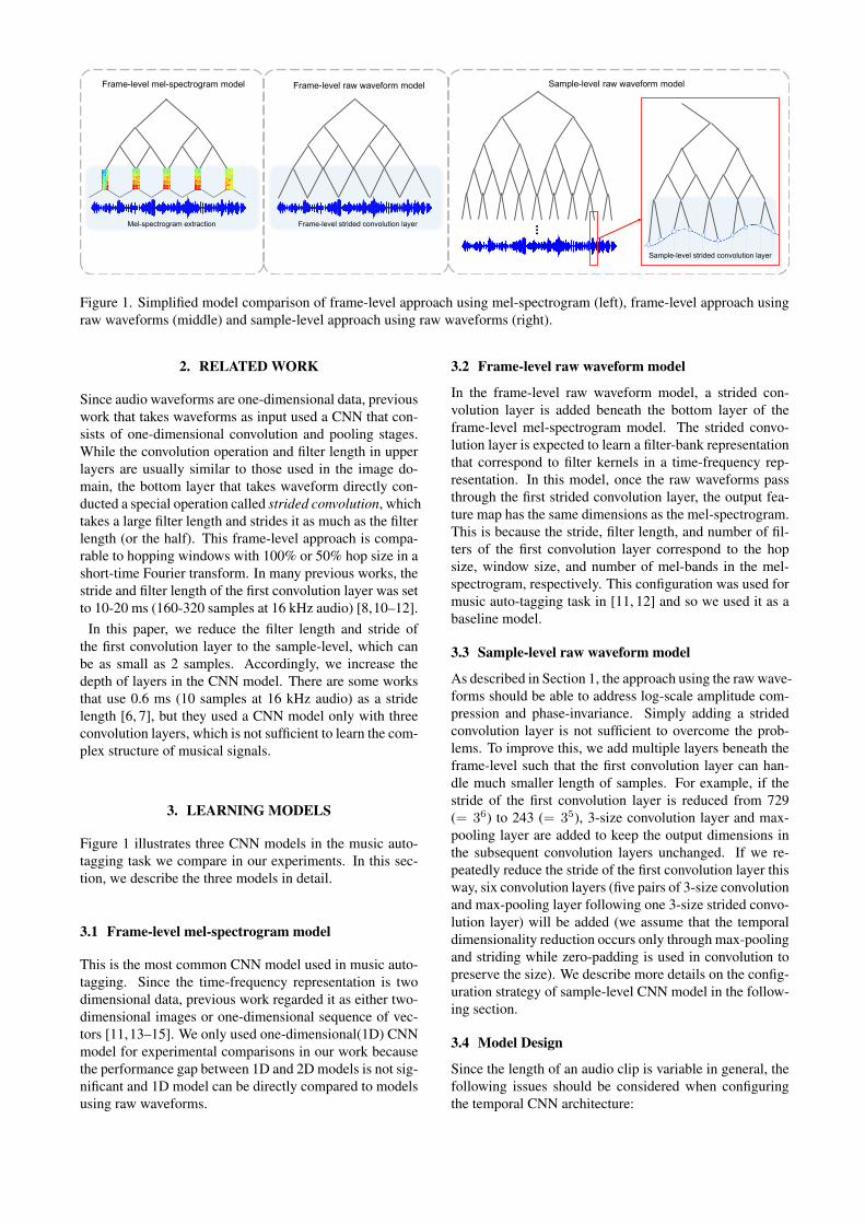
Figure 1. Simplified model comparison of frame-level approach using mel-spectrogram (left), frame-level approach usingraw waveforms (middle) and sample-level approach using raw waveforms (right).

2. RELATED WORK

Since audio waveforms are one-dimensional data, previouswork that takes waveforms as input used a CNN that con-sists of one-dimensional convolution and pooling stages.While the convolution operation and filter length in upperlayers are usually similar to those used in the image do-main, the bottom layer that takes waveform directly con-ducted a special operation called strided convolution, whichtakes a large filter length and strides it as much as the filterlength (or the half). This frame-level approach is compa-rable to hopping windows with 100% or 50% hop size in ashort-time Fourier transform. In many previous works, thestride and filter length of the first convolution layer was setto 10-20 ms (160-320 samples at 16 kHz audio) [8,10–12].

In this paper, we reduce the filter length and stride ofthe first convolution layer to the sample-level, which canbe as small as 2 samples. Accordingly, we increase thedepth of layers in the CNN model. There are some worksthat use 0.6 ms (10 samples at 16 kHz audio) as a stridelength [6, 7], but they used a CNN model only with threeconvolution layers, which is not sufficient to learn the com-plex structure of musical signals.

3. LEARNING MODELS

Figure 1 illustrates three CNN models in the music auto-tagging task we compare in our experiments. In this sec-tion, we describe the three models in detail.

3.1 Frame-level mel-spectrogram model

This is the most common CNN model used in music auto-tagging. Since the time-frequency representation is twodimensional data, previous work regarded it as either two-dimensional images or one-dimensional sequence of vec-tors [11,13–15]. We only used one-dimensional(1D) CNNmodel for experimental comparisons in our work becausethe performance gap between 1D and 2D models is not sig-nificant and 1D model can be directly compared to modelsusing raw waveforms.

3.2 Frame-level raw waveform model

In the frame-level raw waveform model, a strided con-volution layer is added beneath the bottom layer of theframe-level mel-spectrogram model. The strided convo-lution layer is expected to learn a filter-bank representationthat correspond to filter kernels in a time-frequency rep-resentation. In this model, once the raw waveforms passthrough the first strided convolution layer, the output fea-ture map has the same dimensions as the mel-spectrogram.This is because the stride, filter length, and number of fil-ters of the first convolution layer correspond to the hopsize, window size, and number of mel-bands in the mel-spectrogram, respectively. This configuration was used formusic auto-tagging task in [11, 12] and so we used it as abaseline model.

3.3 Sample-level raw waveform model

As described in Section 1, the approach using the raw wave-forms should be able to address log-scale amplitude com-pression and phase-invariance. Simply adding a stridedconvolution layer is not sufficient to overcome the prob-lems. To improve this, we add multiple layers beneath theframe-level such that the first convolution layer can han-dle much smaller length of samples. For example, if thestride of the first convolution layer is reduced from 729(= 36) to 243 (= 35), 3-size convolution layer and max-pooling layer are added to keep the output dimensions inthe subsequent convolution layers unchanged. If we re-peatedly reduce the stride of the first convolution layer thisway, six convolution layers (five pairs of 3-size convolutionand max-pooling layer following one 3-size strided convo-lution layer) will be added (we assume that the temporaldimensionality reduction occurs only through max-poolingand striding while zero-padding is used in convolution topreserve the size). We describe more details on the config-uration strategy of sample-level CNN model in the follow-ing section.

3.4 Model Design

Since the length of an audio clip is variable in general, thefollowing issues should be considered when configuringthe temporal CNN architecture:

• Convolution filter length and sub-sampling length

• The temporal length of hidden layer activations onthe last sub-sampling layer

• The segment length of audio that corresponds to theinput size of the network

First, we attempted a very small filter length in convolu-tional layers and sub-sampling length, following the VGGnet that uses filters of 3× 3 size and max-pooling of 2× 2size [2]. Since we use one-dimensional convolution andsub-sampling for raw waveforms, however, the filter lengthand pooling length need to be varied. We thus constructedseveral DCNN models with different filter length and pool-ing length from 2 to 5, and verified the effect on musicauto-tagging performance. As a sub-sampling method, max-pooling is generally used. Although sub-sampling usingstrided convolution has recently been proposed in a gen-erative model [9], our preliminary test showed that max-pooling was superior to the stride sub-sampling method. Inaddition, to avoid exhausting model search, a pair of sin-gle convolution layer and max-pooling layer with the samesize was used as a basic building module of the DCNN.

Second, the temporal length of hidden layer activationson the last sub-sampling layer reflects the temporal com-pression of the input audio by successive sub-sampling.We set the CNN models such that the temporal length ofhidden layer activation is one. By building the models thisway, we can significantly reduce the number of parametersbetween the last sub-sampling layer and the output layer.Also, we can examine the performance only by the depthof layers and the stride of first convolution layer.

Third, in music classification tasks, the input size of thenetwork is an important parameter that determines the clas-sification performance [16, 17]. In the mel-spectrogrammodel, one song is generally divided into small segmentswith 1 to 4 seconds. The segments are used as the input fortraining and the predictions over all segments in one songare averaged in testing. In the models that use raw wave-form, the learning ability according to the segment size hasbeen not reported yet and thus we need to examine differ-ent input sizes when we configure the CNN models.

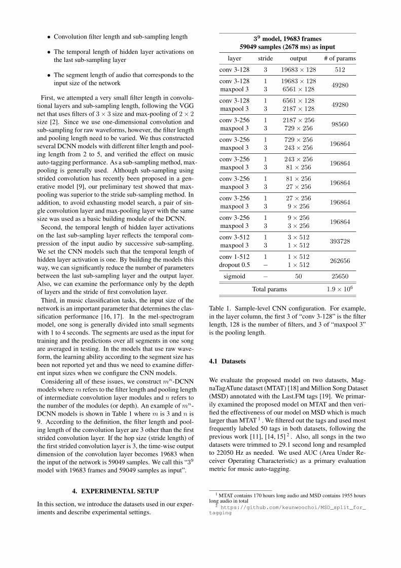
Considering all of these issues, we construct mn-DCNNmodels where m refers to the filter length and pooling lengthof intermediate convolution layer modules and n refers tothe number of the modules (or depth). An example of mn-DCNN models is shown in Table 1 where m is 3 and n is9. According to the definition, the filter length and pool-ing length of the convolution layer are 3 other than the firststrided convolution layer. If the hop size (stride length) ofthe first strided convolution layer is 3, the time-wise outputdimension of the convolution layer becomes 19683 whenthe input of the network is 59049 samples. We call this “39

model with 19683 frames and 59049 samples as input”.

4. EXPERIMENTAL SETUP

In this section, we introduce the datasets used in our exper-iments and describe experimental settings.

39 model, 19683 frames59049 samples (2678 ms) as input

layer stride output # of params

conv 3-128 3 19683× 128 512

conv 3-128maxpool 3

13

19683× 1286561× 128

49280

conv 3-128maxpool 3

13

6561× 1282187× 128

49280

conv 3-256maxpool 3

13

2187× 256729× 256

98560

conv 3-256maxpool 3

13

729× 256243× 256

196864

conv 3-256maxpool 3

13

243× 25681× 256

196864

conv 3-256maxpool 3

13

81× 25627× 256

196864

conv 3-256maxpool 3

13

27× 2569× 256

196864

conv 3-256maxpool 3

13

9× 2563× 256

196864

conv 3-512maxpool 3

13

3× 5121× 512

393728

conv 1-512dropout 0.5

1−

1× 5121× 512

262656

sigmoid − 50 25650

Total params 1.9× 106

Table 1. Sample-level CNN configuration. For example,in the layer column, the first 3 of “conv 3-128” is the filterlength, 128 is the number of filters, and 3 of “maxpool 3”is the pooling length.

4.1 Datasets

We evaluate the proposed model on two datasets, Mag-naTagATune dataset (MTAT) [18] and Million Song Dataset(MSD) annotated with the Last.FM tags [19]. We primar-ily examined the proposed model on MTAT and then veri-fied the effectiveness of our model on MSD which is muchlarger than MTAT 1 . We filtered out the tags and used mostfrequently labeled 50 tags in both datasets, following theprevious work [11], [14, 15] 2 . Also, all songs in the twodatasets were trimmed to 29.1 second long and resampledto 22050 Hz as needed. We used AUC (Area Under Re-ceiver Operating Characteristic) as a primary evaluationmetric for music auto-tagging.

1 MTAT contains 170 hours long audio and MSD contains 1955 hourslong audio in total

2 https://github.com/keunwoochoi/MSD_split_for_tagging

https://github.com/keunwoochoi/MSD_split_for_tagging

https://github.com/keunwoochoi/MSD_split_for_tagging

2n models

model with 16384 samples (743 ms) as input model with 32768 samples (1486 ms) as input

model n layer filter length & stride AUC model n layer filter length & stride AUC

64 frames 6 1+6+1 256 0.8839 128 frames 7 1+7+1 256 0.8834128 frames 7 1+7+1 128 0.8899 256 frames 8 1+8+1 128 0.8872256 frames 8 1+8+1 64 0.8968 512 frames 9 1+9+1 64 0.8980512 frames 9 1+9+1 32 0.8994 1024 frames 10 1+10+1 32 0.8988


3n models




2187 frames 7 1+7+1 9 0.9033 6561 frames 8 1+8+1 9 0.90306561 frames 8 1+8+1 3 0.9039 19683 frames 9 1+9+1 3 0.9055

4n models





5n models




3125 frames 5 1+5+1 5 0.9024 15625 frames 6 1+6+1 5 0.9041

Table 2. Comparison of various mn-DCNN models with different input sizes. m refers to the filter length and pooling lengthof intermediate convolution layer modules and n refers to the number of the modules. Filter length & stride indicates thevalue of the first convolution layer. In the layer column, the first digit ’1’ of 1+n+1 is the strided convolution layer, and thelast digit ’1’ is convolution layer which actually works as a fully-connected layer.

4.2 Optimization

We used sigmoid activation for the output layer and bi-nary cross entropy loss as the objective function to opti-mize. For every convolution layer, we used batch normal-ization [20] and ReLU activation. We should note that, inour experiments, batch normalization plays a vital role intraining the deep models that takes raw waveforms. Weapplied dropout of 0.5 to the output of the last convolutionlayer and minimized the objective function using stochas-tic gradient descent with 0.9 Nesterov momentum. Thelearning rate was initially set to 0.01 and decreased by afactor of 5 when the validation loss did not decrease morethan 3 epochs. A total decrease of 4 times, the learning rateof the last training was 0.000016. Also, we used batch size

of 23 for MTAT and 50 for MSD, respectively. In the mel-spectrogram model, we conducted the input normalizationsimply by dividing the standard deviation after subtractingmean value of entire input data. On the other hand, we didnot perform the input normalization for raw waveforms.

5. RESULTS

In this section, we examine the proposed models and com-pare them to previous state-of-the-art results.

5.1 mn-DCNN models

Table 2 shows the evaluation results for the mn-DCNNmodels on MTAT for different input sizes, number of lay-ers, filter length and stride of the first convolution layer. As

3n models,59049 samples

as inputn

window(filter length)

hop(stride) AUC

Frame-level(mel-spectrogram)

4 729 729 0.90005 729 243 0.90055 243 243 0.90476 243 81 0.90596 81 81 0.9025

Frame-level(raw waveforms)

4 729 729 0.86555 729 243 0.87425 243 243 0.88236 243 81 0.89066 81 81 0.8936

Sample-level(raw waveforms)

7 27 27 0.90028 9 9 0.90309 3 3 0.9055

Table 3. Comparison of three CNN models with differ-ent window (filter length) and hop (stride) sizes. n rep-resents the number of intermediate convolution and max-pooling layer modules, thus 3n times hop (stride) size ofeach model is equal to the number of input samples.

input type model MTAT MSD

Frame-level(mel-spectrogram)

Persistent CNN [21] 0.9013 -2D CNN [14] 0.894 0.851CRNN [15] - 0.862

Proposed DCNN 0.9059 -

Frame-level(raw waveforms) 1D CNN [11] 0.8487 -

Sample-level(raw waveforms) Proposed DCNN 0.9055 0.8812

Table 4. Comparison of our works to prior state-of-the-arts

described in Section 3.4, m refers to the filter length andpooling length of intermediate convolution layer modulesand n refers to the number of the modules. In Table 2,we can first find that the accuracy is proportional to n formost m. Increasing n given m and input size indicates thatthe filter length and stride of the first convolution layer be-come closer to the sample-level (e.g. 2 or 3 size). When thefirst layer reaches the small granularity, the architecture isseen as a model constructed with the same filter length andsub-sampling length in all convolution layers as depictedin Table 1. The best results were obtained when m was 3and n was 9. Interestingly, the length of 3 corresponds tothe 3-size spatial filters in the VGG net [2]. In addition, wecan see that 1-3 seconds of audio as an input length to thenetwork is a reasonable choice in the raw waveform modelas in the mel-spectrogram model.

5.2 Mel-spectrogram and raw waveforms

Considering that the output size of the first convolutionlayer in the raw waveform models is equivalent to the mel-spectrogram size, we further validate the effectiveness of

the proposed sample-level architecture by performing ex-periments presented in Table 3. The models used in theexperiments follow the configuration strategy described inSection 3.4. In the mel-spectrogram experiments, 128 mel-bands are used to match up to the number of filters in thefirst convolution layer of the raw waveform model. FFTsize was set to 729 in all comparisons and the magnitudecompression is applied with a nonlinear curve, log(1 +C|A|) where A is the magnitude and C is set to 10.

The results in Table 3 show that the sample-level rawwaveform model achieves results comparable to the frame-level mel-spectrogram model. Specifically, we found thatusing a smaller hop size (81 samples ≈ 4 ms) worked bet-ter than those of conventional approaches (about 20 ms orso) in the frame-level mel-spectrogram model. However,if the hop size is less than 4 ms, the performance degraded.An interesting finding from the result of the frame-levelraw waveform model is that when the filter length is largerthan the stride, the accuracy is slightly lower than the mod-els with the same filter length and stride. We interpret thatthis result is due to the learning ability of the phase vari-ance. As the filter length decreases, the extent of phasevariance that the filters should learn is reduced.

5.3 MSD result and the number of filters

We investigate the capacity of our sample-level architec-ture even further by evaluating the performance on MSDthat is ten times larger than MTAT. The result is shown inTable 4. While training the network on MSD, the numberof filters in the convolution layers has been shown to affectthe performance. According to our preliminary test results,increasing the number of filters from 16 to 512 along thelayers was sufficient for MTAT. However, the test on MSDshows that increasing the number of filters in the first con-volution layer improves the performance. Therefore, weincreased the number of filters in the first convolution layerfrom 16 to 128.

5.4 Comparison to state-of-the-arts

In Table 4, we show the performance of the proposed ar-chitecture to previous state-of-the-arts on MTAT and MSD.They show that our proposed sample-level architecture ishighly effective compared to them.

5.5 Visualization of learned filters

The technique of visualizing the filters learned at each layerallows better understanding of representation learning inthe hierarchical network. However, many previous worksin music domain are limited to visualizing learned filtersonly on the first convolution layer [11, 12].

The gradient ascent method has been proposed for filtervisualization [22] and this technique has provided deeperunderstanding of what convolutional neural networks learnfrom images [23, 24]. We applied the technique to ourDCNN to observe how each layer hears the raw wave-forms. The gradient ascent method is as follows. First, wegenerate random noise and back-propagate the errors in thenetwork. The loss is set to the target filter activation. Then,

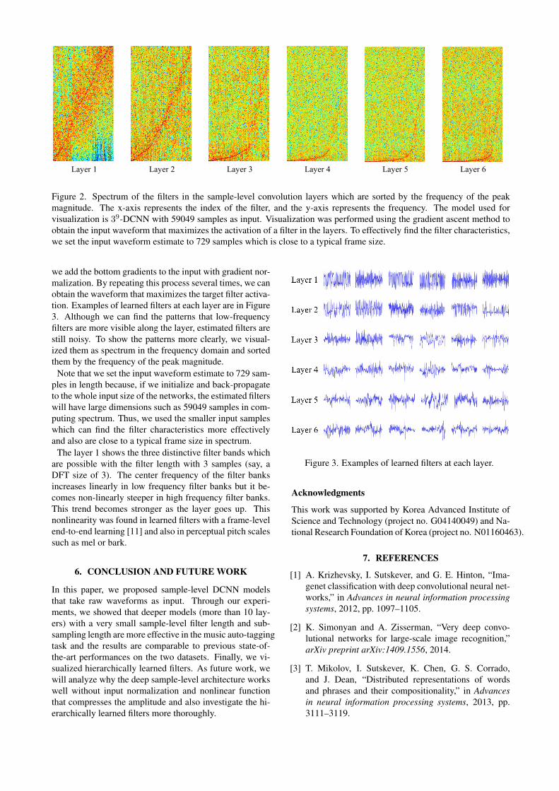
Layer 1 Layer 2 Layer 3 Layer 4 Layer 5 Layer 6

Figure 2. Spectrum of the filters in the sample-level convolution layers which are sorted by the frequency of the peakmagnitude. The x-axis represents the index of the filter, and the y-axis represents the frequency. The model used forvisualization is 39-DCNN with 59049 samples as input. Visualization was performed using the gradient ascent method toobtain the input waveform that maximizes the activation of a filter in the layers. To effectively find the filter characteristics,we set the input waveform estimate to 729 samples which is close to a typical frame size.

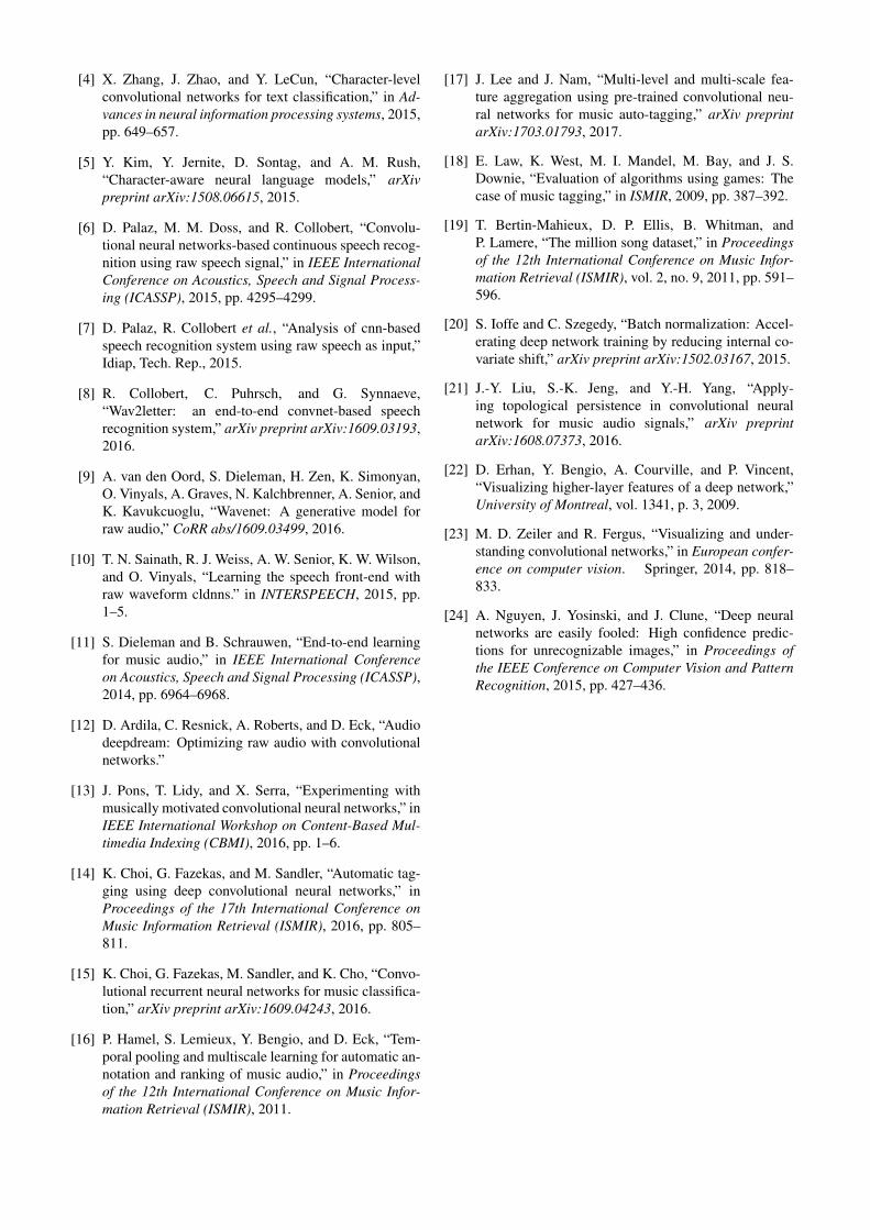
we add the bottom gradients to the input with gradient nor-malization. By repeating this process several times, we canobtain the waveform that maximizes the target filter activa-tion. Examples of learned filters at each layer are in Figure3. Although we can find the patterns that low-frequencyfilters are more visible along the layer, estimated filters arestill noisy. To show the patterns more clearly, we visual-ized them as spectrum in the frequency domain and sortedthem by the frequency of the peak magnitude.

Note that we set the input waveform estimate to 729 sam-ples in length because, if we initialize and back-propagateto the whole input size of the networks, the estimated filterswill have large dimensions such as 59049 samples in com-puting spectrum. Thus, we used the smaller input sampleswhich can find the filter characteristics more effectivelyand also are close to a typical frame size in spectrum.

The layer 1 shows the three distinctive filter bands whichare possible with the filter length with 3 samples (say, aDFT size of 3). The center frequency of the filter banksincreases linearly in low frequency filter banks but it be-comes non-linearly steeper in high frequency filter banks.This trend becomes stronger as the layer goes up. Thisnonlinearity was found in learned filters with a frame-levelend-to-end learning [11] and also in perceptual pitch scalessuch as mel or bark.

6. CONCLUSION AND FUTURE WORK

In this paper, we proposed sample-level DCNN modelsthat take raw waveforms as input. Through our experi-ments, we showed that deeper models (more than 10 lay-ers) with a very small sample-level filter length and sub-sampling length are more effective in the music auto-taggingtask and the results are comparable to previous state-of-the-art performances on the two datasets. Finally, we vi-sualized hierarchically learned filters. As future work, wewill analyze why the deep sample-level architecture workswell without input normalization and nonlinear functionthat compresses the amplitude and also investigate the hi-erarchically learned filters more thoroughly.

Figure 3. Examples of learned filters at each layer.

Acknowledgments

This work was supported by Korea Advanced Institute ofScience and Technology (project no. G04140049) and Na-tional Research Foundation of Korea (project no. N01160463).

7. REFERENCES

[1] A. Krizhevsky, I. Sutskever, and G. E. Hinton, “Ima-genet classification with deep convolutional neural net-works,” in Advances in neural information processingsystems, 2012, pp. 1097–1105.

[2] K. Simonyan and A. Zisserman, “Very deep convo-lutional networks for large-scale image recognition,”arXiv preprint arXiv:1409.1556, 2014.

[3] T. Mikolov, I. Sutskever, K. Chen, G. S. Corrado,and J. Dean, “Distributed representations of wordsand phrases and their compositionality,” in Advancesin neural information processing systems, 2013, pp.3111–3119.

[4] X. Zhang, J. Zhao, and Y. LeCun, “Character-levelconvolutional networks for text classification,” in Ad-vances in neural information processing systems, 2015,pp. 649–657.

[5] Y. Kim, Y. Jernite, D. Sontag, and A. M. Rush,“Character-aware neural language models,” arXivpreprint arXiv:1508.06615, 2015.

[6] D. Palaz, M. M. Doss, and R. Collobert, “Convolu-tional neural networks-based continuous speech recog-nition using raw speech signal,” in IEEE InternationalConference on Acoustics, Speech and Signal Process-ing (ICASSP), 2015, pp. 4295–4299.

[7] D. Palaz, R. Collobert et al., “Analysis of cnn-basedspeech recognition system using raw speech as input,”Idiap, Tech. Rep., 2015.

[8] R. Collobert, C. Puhrsch, and G. Synnaeve,“Wav2letter: an end-to-end convnet-based speechrecognition system,” arXiv preprint arXiv:1609.03193,2016.

[9] A. van den Oord, S. Dieleman, H. Zen, K. Simonyan,O. Vinyals, A. Graves, N. Kalchbrenner, A. Senior, andK. Kavukcuoglu, “Wavenet: A generative model forraw audio,” CoRR abs/1609.03499, 2016.

[10] T. N. Sainath, R. J. Weiss, A. W. Senior, K. W. Wilson,and O. Vinyals, “Learning the speech front-end withraw waveform cldnns.” in INTERSPEECH, 2015, pp.1–5.

[11] S. Dieleman and B. Schrauwen, “End-to-end learningfor music audio,” in IEEE International Conferenceon Acoustics, Speech and Signal Processing (ICASSP),2014, pp. 6964–6968.

[12] D. Ardila, C. Resnick, A. Roberts, and D. Eck, “Audiodeepdream: Optimizing raw audio with convolutionalnetworks.”

[13] J. Pons, T. Lidy, and X. Serra, “Experimenting withmusically motivated convolutional neural networks,” inIEEE International Workshop on Content-Based Mul-timedia Indexing (CBMI), 2016, pp. 1–6.

[14] K. Choi, G. Fazekas, and M. Sandler, “Automatic tag-ging using deep convolutional neural networks,” inProceedings of the 17th International Conference onMusic Information Retrieval (ISMIR), 2016, pp. 805–811.

[15] K. Choi, G. Fazekas, M. Sandler, and K. Cho, “Convo-lutional recurrent neural networks for music classifica-tion,” arXiv preprint arXiv:1609.04243, 2016.

[16] P. Hamel, S. Lemieux, Y. Bengio, and D. Eck, “Tem-poral pooling and multiscale learning for automatic an-notation and ranking of music audio,” in Proceedingsof the 12th International Conference on Music Infor-mation Retrieval (ISMIR), 2011.

[17] J. Lee and J. Nam, “Multi-level and multi-scale fea-ture aggregation using pre-trained convolutional neu-ral networks for music auto-tagging,” arXiv preprintarXiv:1703.01793, 2017.

[18] E. Law, K. West, M. I. Mandel, M. Bay, and J. S.Downie, “Evaluation of algorithms using games: Thecase of music tagging,” in ISMIR, 2009, pp. 387–392.

[19] T. Bertin-Mahieux, D. P. Ellis, B. Whitman, andP. Lamere, “The million song dataset,” in Proceedingsof the 12th International Conference on Music Infor-mation Retrieval (ISMIR), vol. 2, no. 9, 2011, pp. 591–596.

[20] S. Ioffe and C. Szegedy, “Batch normalization: Accel-erating deep network training by reducing internal co-variate shift,” arXiv preprint arXiv:1502.03167, 2015.

[21] J.-Y. Liu, S.-K. Jeng, and Y.-H. Yang, “Apply-ing topological persistence in convolutional neuralnetwork for music audio signals,” arXiv preprintarXiv:1608.07373, 2016.

[22] D. Erhan, Y. Bengio, A. Courville, and P. Vincent,“Visualizing higher-layer features of a deep network,”University of Montreal, vol. 1341, p. 3, 2009.

[23] M. D. Zeiler and R. Fergus, “Visualizing and under-standing convolutional networks,” in European confer-ence on computer vision. Springer, 2014, pp. 818–833.

[24] A. Nguyen, J. Yosinski, and J. Clune, “Deep neuralnetworks are easily fooled: High confidence predic-tions for unrecognizable images,” in Proceedings ofthe IEEE Conference on Computer Vision and PatternRecognition, 2015, pp. 427–436.

sample-level deep convolutional neural networks for music ... · sample-level deep convolutional...

Documents