rubik's cube: an energy perspective
TRANSCRIPT

PHYSICAL REVIEW E 89, 012815 (2014)
Rubik’s cube: An energy perspective
Yiing-Rei ChenDepartment of Physics, National Taiwan Normal University, Taipei 11677, Taiwan
Chi-Lun Lee*
Department of Physics, National Central University, Jhongli 32001, Taiwan(Received 16 October 2013; published 29 January 2014)
What if we played the Rubik’s cube game by simple intuition? We would rotate the cube, probably in the hopeof getting a more organized pattern in each next step. Yet frustration occurs easily, and we soon find ourselvestrapped as the game progresses no further. Played in this completely strategy-less style, the entire problem of theRubik’s cube game can be compared to that of complex chemical reactions such as protein folding, only withless guidance in the searching process. In this work we look into this random-searching process by means ofthermodynamics and compare the game’s dynamics with that of a faithful stochastic model constructed from thestatistical energy landscape theory (SELT). This comparison reveals the peculiar nature of SELT, which relieson the random energy approximation and often chops up energy correlations among nearby configurations. Ourobservation provides a general insight for the use of SELT in the studies of these frustrated systems.
DOI: 10.1103/PhysRevE.89.012815 PACS number(s): 82.20.−w
I. INTRODUCTION
Rubik’s cube has drawn long-lasting interest from thegeneral public as well as the scientific community since itsbirth in the 1970s [1]. The cube itself bears a concise physicalstructure and is operated with basic rotational rules. Yet itappears difficult for most players to solve the cube toward itsultimate, ordered pattern. The vast number of configurations(of the order of 1019), along with the rotations that serve astheir links, form a network that has a regular structure, in thesense that each configuration is linked to an identical numberof nearest neighbors. In spite of the numerous configurations,it has been proven recently that the shortest path betweenany two configurations contains no more than 20 steps [2],each step standing for a rotation of some face by 90◦ or 180◦,clockwise or counterclockwise [3].
Aside from the elegance of its mathematical structure[4], the Rubik’s cube game, when played with a very naiveattitude, leads to experiences that are strikingly similar to thosewith the famous protein-folding problem [5]. The similaritymainly lies in the frustration during the global minimumsearching process, and this frustration is attributed to the lackof farsighted guidance and the misleading local traps. In theprotein-folding problem, however, the searching process canbe suddenly sped up as guided sequential moves are triggered,such as zipping or helical structure formation, which followsthe so-called “cooperative” nature [6–8], an essence due tothe chain-connecting structure in proteins. The lack of suchessence in the Rubik’s cube problem leads to a slower, morerandom searching process, where single rotations are oftenaccompanied by huge energy leaps. In fact, following thecommonly used Monte Carlo simulation procedure [9], fora standard 3 × 3 × 3 Rubik’s cube it is almost impossibleto reach the ultimate pattern within a reasonable computingtime. In the current study, we choose to use a simplified energyfunction that ignores the edge patches of the cube, so as to make
computer simulations and energy landscape analysis [10,11]possible.
From our previous study [12], we have demonstrated thatthe Rubik’s cube problem, if viewed from the thermodynamicperspective, exhibits a peak in heat capacity. This peakrepresents the existence of a transition between the native state,which represents the configuration for the energy optimum,and the disordered state, which stands for the vast number ofdisordered configurations. This feature alone bears a strikingresemblance to the folding transition of the protein problem.Moreover, via Monte Carlo simulations we find that the meanfirst-passage time (MFPT) [13] exhibits a U-shaped trendversus temperature. This indicates that the searching processtowards the native state gets much faster at the optimizedtemperature than an unguided search throughout the wholeconfiguration space [14]. From a statistical study we haveconfirmed that the energy landscape has a bias towards thenative state, while the nature for the frustrated landscape is bestexhibited through a nonexponential relaxation in the energyautocorrelation function. All of these results coincide well withthe corresponding observations in protein-folding research.Despite this analogy, we should point out that the Rubik’scube problem, having a highly simplified structure, possessesa relatively tiny funnel-like region in its energy landscape,which results in a more diffusive searching process than theprotein-folding dynamics.
In the protein science community, studies concerning suchbumpy energy landscapes are often performed with the aid ofthe statistical energy landscape theory (SELT) [10,15], wherethe numerous configurations as well as their detailed reactionlinks are parameterized by one or a few reaction coordinates.After being projected onto these reaction coordinates, the hugeamount of configurational information is transformed into astatistical distribution that establishes the stochastic natureof the theoretically rebuilt model, which features a randomenergy Hamiltonian [16,17]. Originally developed for studieson protein folding without consideration of cooperativity[15,18], SELT is, in our perspective, a very promising toolfor describing the Rubik’s cube problem.
1539-3755/2014/89(1)/012815(6) 012815-1 ©2014 American Physical Society
YIING-REI CHEN AND CHI-LUN LEE PHYSICAL REVIEW E 89, 012815 (2014)
In the spirit of methodologic study, we construct SELTin the current work as a rebuilt version of the Rubik’scube model (RCM) we use, and examine the similarity anddissimilarity between the two. Regarding the MFPT, theMonte Carlo simulations performed for both models show thesame qualitative features that characterize the protein-foldingdynamics. In particular, the MFPT results from both modelsagree well quantitatively in the high-temperature regime. Tounderstand the numerical discrepancy that increases at lowtemperatures, we examine the energy-time series and find thefrozen movements peculiar to the random walker of SELT.We point out from there the essential difference between thedynamic behaviors with the two models. In short, while RCM’srandom walker pays more short-term visits to secondaryminima, SELT’s random walker seldom encounters the “trapstates” but gets frozen there once it steps in. Moreover, theentrapment in SELT is both energetic and entropic, whichleads to a very different temperature dependence in its dynamicbehavior.
II. MODELS AND METHODS
In this work we use a simplified 3 × 3 × 3 RCM, where weignore the edge patches and only consider the colors of cornerpatches and face-center patches in the energy function. Foreach configuration of this model, the corresponding energy isdefined by E = −∑6
i=1 ni , where the summation runs over allsix faces of the cube, and ni is the number of corner patchesthat sit on the ith face and share the same color with thecentral patch of that face. The lowest energy of the cube istherefore −24, which corresponds to the ultimate configurationwhere all six faces are solid colored. Following the languageof protein-folding dynamics, we choose to call this ultimateconfiguration the “native state.”
Once the energy function is defined, one can rephrase theRubik’s cube problem in the language of thermodynamics. Inparticular, its kinetic behavior under a constant-temperatureheat bath can be established using the Metropolis Monte Carloalgorithm [9]. For each Monte Carlo time step, a move ispicked from a total of 12 rotations, whereas a “rotation” meanspicking a face and rotating the layer of pieces underneaththat picked face by 90◦, clockwise or counterclockwise.Whether this move is actually performed is determined by theMetropolis algorithm, to assure the detailed-balance conditionupon thermodynamic equilibrium. For simplicity, we usedimensionless units for energy and temperature and takekB ≡ 1 for the Boltzmann constant.
To help grab a taste of the “game progress,’ as if in protein-folding problems, we define an order parameter ρ that labelsthe distance, namely, the minimal number of rotations, towardsthe native state. The vast number of configurations of RCMcan be classified by their ρ numbers, which are no larger than14. Subsequently, statistical information such as the energyprobability distribution P (E,ρ) and the total number of linksbetween successive ρ’s can then be derived.
In particular, the projection from the configuration spaceonto the ρ axis leads us to the construction of SELT viathe random energy approximation. In RCM, each specificrotation forms a link between a certain configuration of ρ
and another of ρ ± 1, with no ambiguity [19]. In other words,
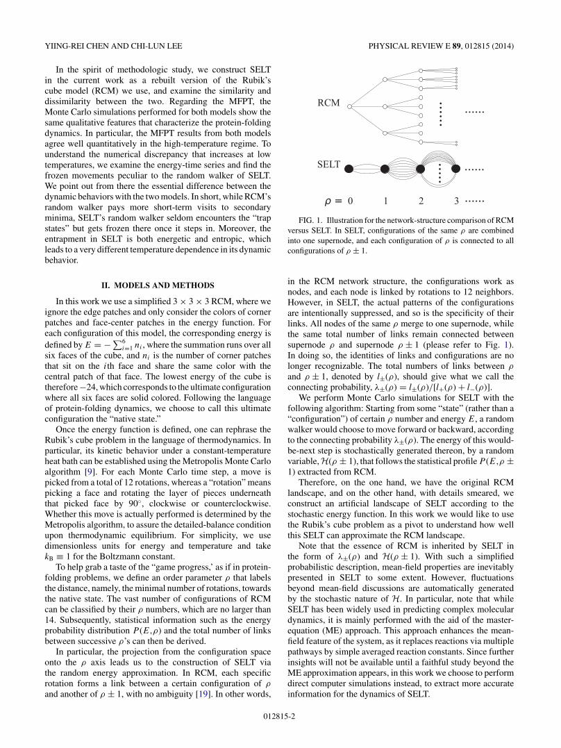
FIG. 1. Illustration for the network-structure comparison of RCMversus SELT. In SELT, configurations of the same ρ are combinedinto one supernode, and each configuration of ρ is connected to allconfigurations of ρ ± 1.
in the RCM network structure, the configurations work asnodes, and each node is linked by rotations to 12 neighbors.However, in SELT, the actual patterns of the configurationsare intentionally suppressed, and so is the specificity of theirlinks. All nodes of the same ρ merge to one supernode, whilethe same total number of links remain connected betweensupernode ρ and supernode ρ ± 1 (please refer to Fig. 1).In doing so, the identities of links and configurations are nolonger recognizable. The total numbers of links between ρ
and ρ ± 1, denoted by l±(ρ), should give what we call theconnecting probability, λ±(ρ) = l±(ρ)/[l+(ρ) + l−(ρ)].
We perform Monte Carlo simulations for SELT with thefollowing algorithm: Starting from some “state” (rather than a“configuration”) of certain ρ number and energy E, a randomwalker would choose to move forward or backward, accordingto the connecting probability λ±(ρ). The energy of this would-be-next step is stochastically generated thereon, by a randomvariable,H(ρ ± 1), that follows the statistical profile P (E,ρ ±1) extracted from RCM.
Therefore, on the one hand, we have the original RCMlandscape, and on the other hand, with details smeared, weconstruct an artificial landscape of SELT according to thestochastic energy function. In this work we would like to usethe Rubik’s cube problem as a pivot to understand how wellthis SELT can approximate the RCM landscape.
Note that the essence of RCM is inherited by SELT inthe form of λ±(ρ) and H(ρ ± 1). With such a simplifiedprobabilistic description, mean-field properties are inevitablypresented in SELT to some extent. However, fluctuationsbeyond mean-field discussions are automatically generatedby the stochastic nature of H. In particular, note that whileSELT has been widely used in predicting complex moleculardynamics, it is mainly performed with the aid of the master-equation (ME) approach. This approach enhances the mean-field feature of the system, as it replaces reactions via multiplepathways by simple averaged reaction constants. Since furtherinsights will not be available until a faithful study beyond theME approximation appears, in this work we choose to performdirect computer simulations instead, to extract more accurateinformation for the dynamics of SELT.
012815-2

RUBIK’s CUBE: AN ENERGY PERSPECTIVE PHYSICAL REVIEW E 89, 012815 (2014)
0 4 8 12ρ
100
102
104
106
108
n(ρ)
-24 -16 -8 0E
100
102
104
106
n(E)
(b)(a)
FIG. 2. Number of configurations versus (a) the order parameterρ and (b) the energy in RCM.
III. RESULTS
The statistics of the RCM configurations, such as the energyprobability distribution P (E,ρ) and the connecting probabilityλ±(ρ), are acquired from our computer exhaustive studies thatbranch out from the native state. There are a total of 88 179 840configurations for our simplified 3 × 3 × 3 cube, and theirstatistic information versus ρ and E is plotted in Fig. 2. Notethat the exponential growth near the native state, as revealed inFigs. 2(a) and 2(b), implies that low-energy (i.e., E < −12) ornative vicinity configurations occupy only a very small fractionof the overall configuration space.
In RCM, the probability distributions of energy change forlinks between ρ and ρ ± 1 are denoted by P ±
RCM(�E,ρ), asplotted in Fig. 3. The corresponding probability distributions
-24 -12 0 12 240
0.5
1
-24 -12 0 12 240
0.5
1
-24 -12 0 12 240
0.10.20.3
-24 -12 0 12 240
0.1
0.2
-24 -12 0 12 240
0.1
0.2
-24 -12 0 12 240
0.1
0.2
-24 -12 0 12 240
0.1
0.2
-24 -12 0 12 240
0.1
0.2
-24 -12 0 12 240
0.1
0.2
-24 -12 0 12 240
0.1
0.2
-24 -12 0 12 240
0.1
0.2
-24 -12 0 12 240
0.1
0.2
-24 -12 0 12 240
0.1
0.2
-24 -12 0 12 240
0.1
0.2
ΔE
prob
abili
ty
ρ=2
ρ=3 ρ=4 ρ=5
ρ=6
ρ=9 ρ=10 ρ=11
ρ=12 ρ=13
ρ=1ρ=0
ρ=7 ρ=8
FIG. 3. (Color) Probability distributions over energy change.Only plots for forward motions of ρ → ρ + 1 are listed. As forbackward motions of ρ → ρ − 1, the distribution is just the reflectionof plot ρ − 1 → ρ over axis �E = 0. Red, RCM; blue, SELT.
in SELT are given by
P ±SELT(�E,ρ) ≡
∑
E1,E2
P (E1,ρ)P (E2,ρ ± 1)δE2−E1,�E. (1)
We see in Fig. 3 that for ρ < 3 the probability distributioncreated in SELT shows little difference from that in RCM.Furthermore, the observation that both PRCM(�E,ρ) andPSELT(�E,ρ) resemble a Gaussian distribution for ρ > 3 leadsto an intuitive speculation that, despite the specificity in itsconfiguration structure, RCM gives rise to such uncorrelatedprofiles for energy change between consecutive steps, and therandom-energy hypothesis in SELT is, after all, well supportedin this aspect. Nevertheless, by comparison we find thatPSELT(�E,ρ) is, in general, broader then PRCM(�E,ρ), whichmanifests the artifact produced by stochastically assignedconnections.
We now turn to a discussion of dynamics by first looking atthe MFPT towards the native state. As derived in our previouswork [12] on RCM simulations and the parallel study withan ME approximation, the MFPT curves exhibit a U-shapedfeature (called “chevron rollover” in the studies of protein-folding dynamics [20]), and the slow dynamics in the high-and low-temperature regimes shown therein can be accountedfor by the tedious random-searching process and the existenceof deep energy traps, respectively. In the ME approximation[12], the dynamics is mapped to a one-dimensional diffusionprocess along ρ, where transitions between successive ρ’s arerepresented by the average reaction rates,
kρ,ρ±1 =∑
E
∑
E′P (E,ρ)P (E′,ρ ± 1)k(E → E′), (2)
and k(E → E′) is the transition rate between two configura-tions via the Metropolis algorithm.
With the new MFPT result in this work, we first makea comparison between the ME approximation and SELT, interms of how much they preserve and reveal for the dynamicmessage in RCM simulations. As shown in Fig. 4, the MEapproach underestimates the reaction dynamics, especiallyat low temperatures. This can be easily explained: whenthe approach described in Eq. (2) is applied, the kineticsof all configuration links are averaged. Since deep energytraps are featured by low-rate, low-population processes, theyfail to make any significant contribution to this average.(Alternatively, one may choose to derive for each ρ the leavingrate from the average waiting time, following what is done inthe Bryngelson-Wolynes theory [18,21,22]. In that manner thedynamics of low-lying energy traps would be greatly amplifiedand result in a very slow diffusion process.)
To go beyond the mean-field approach of ME, direct SELTsimulation should serve as a better approximation to RCM,since fluctuation of the kinetic rate is then considered. In fact,it is remarkable to see in Fig. 4 that the MFPT result of SELTfits much better to that of RCM in the high-temperature regime.However, the discrepancy between the two models increasessignificantly at low temperatures. Further study is thereforeneeded to resolve the dynamic distinction between the twomodels.
To look further into the dynamics, we now examine theaverage number of moves during the first-passage (FP) time,
012815-3

YIING-REI CHEN AND CHI-LUN LEE PHYSICAL REVIEW E 89, 012815 (2014)
0 0.5 1 1.5 21/T
102
103
104
105
106
107
108
109
1010M
FPT
RCM (time)SELT (time)ME (time)RCM (moves)SELT (moves)
FIG. 4. (Color online) Results of the mean first-passage time(MFPT). Squares represent SELT data from direct simulations; datafrom RCM simulations (circles) and data from SELT predictionsusing the master-equation (ME) analysis (triangles) were derivedpreviously [12] and are also shown here. Crosses and diamondsmark the average numbers of first-passage (FP) moves for RCM andSELT simulations, respectively. The average is performed for 10 000simulations at each temperature for each model.
as shown in Fig. 4, for RCM and SELT. Note that a “move” isdefined here as an actual change of configuration, and in ourcase, it is also equivalent to an actual change of the randomwalker’s position on the order parameter axis. Surprisingly,while the RCM result still exhibits a U-shaped feature,the average number of moves in SELT shows a monotonicdecrease with 1/T . At T = 0.5 it even becomes less than 1000,almost in scale with the number of moves during the diffusiveMFPT of a nonguided one-dimensional random walk.
The above observation reveals a curious fact, that whilethe random walker in SELT simulations appears to be slow atlow temperatures, it actually spends considerably fewer movessearching for the native state. Figure 5 is a snapshot of theenergy-time series for both simulations at T = 0.7. The ran-dom walker of SELT stays frozen most of the time and, there-fore, gives far fewer details in its dynamics. In other words,the SELT simulations’ success in mimicking the MFPT trendin RCM is in fact based on a very distinct dynamic behavior.
Energy-time series such as the one shown in Fig. 5 canbe used to derive the autocorrelation function CE(t), definedby CE(t) = 〈�E(t)�E(0)〉/〈�E2〉, where �E ≡ E − 〈E〉.Serving as a memory function, CE(t) provides a clearer
0.0 6.0×10⁴ 1.2×10⁵ 1.8×10⁵
time (steps)
-20
-15
-10
-5
0
E
0.0 6.0×10⁴ 1.2×10⁵ 1.8×10⁵
time (steps)
-20
-15
-10
-5
0
E
(a) (b)
FIG. 5. Snapshots of the energy time series for (a) RCM and(b) SELT at T = 0.7.
100 102 104 106
time (steps)
0
0.2
0.4
0.6
0.8
1
CE(t)
RCMSELT
100 102 104 106
time (steps)
0
0.2
0.4
0.6
0.8
1
CE(t)
RCMSELT
(a) (b)
FIG. 6. (Color online) (a) Energy autocorrelation functionsCE(t) for RCM (circles) and SELT (squares) at the equilibrium ofT = 0.7. For each model, the values of CE(t) are obtained from asimulation of 1010 Monte Carlo time steps. (b) Energy autocorrelationfunctions at T = 0.7, acquired from 1000 FP simulations for bothmodels.
perspective for understanding the essentials of the differentdynamic behaviors. In particular, we show the results of CE(t)at T = 0.7, for equilibrium in Fig. 6(a) and for FP processesin Fig. 6(b). The legitimacy of the autocorrelation function inFig. 6(b) is based on the equilibrium provided by the sampledFP cases. As a check, the FP average energy is 〈E〉 = −18.126for RCM and 〈E〉 = −18.121 for SELT, both sitting closelyto the number 〈E〉 = −18.125, derived from the partitionfunction excluding only the native state.
When the native state is excluded, as demonstrated inFig. 6(b), SELT possesses a better memory on all time scalesof interest. The differences between Fig. 6(a) and Fig. 6(b) arecertainly due to the influence of the native state. By includingthis influence, the result of the long-term memory competitionis reversed.
Note that in this example of a relatively low temperature, thekinetics is mainly governed by the random walker’s behaviorin the vicinities of low-energy traps. That is, Fig. 6(b) revealsthe fact that SELT’s walker has a better memory, or, in otherwords, spends a longer time, on low-energy traps, which inturn implies lower probabilities of finding these traps (sinceboth models share the same energy histogram [23]). Indeed,this deduction is echoed by the results of MFPT toward thesecond minima (E = −20), as listed in Table I, where thenumber from SELT simulations is almost 10 times longer thanthat from RCM.
In Table I we also list the equilibrium average energy atT = 0.7, for both SELT and RCM simulations. Note that while〈E〉 is a time-averaged quantity, 〈E〉′ is an average over moves.
TABLE I. Average energies and MFPTs, for RCM and SELTat T = 0.7. For each model, the average energies are derived froma simulation of 1010 time steps. Unprimed data are time-averagedquantities, while primed data are averages over moves. Each MFPTvalue is obtained from 10 000 simulations.
〈E〉 〈E〉′ MFPT
To E = −24 To E = −20
RCM −22.7 −14.9 1.74 × 10⁷ 2.44 × 10⁶
SELT −23.0 −10.7 3.60 × 10⁶ 2.25 × 10⁷
012815-4
RUBIK’s CUBE: AN ENERGY PERSPECTIVE PHYSICAL REVIEW E 89, 012815 (2014)
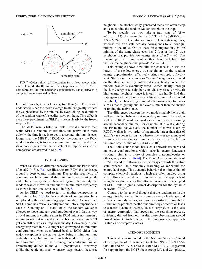
FIG. 7. (Color online) (a) Illustration for a deep energy mini-mum of RCM. (b) Illustration for a trap state of SELT. Circleddots represent the true-neighbor configurations. Links between ρ
and ρ ± 1 are represented by lines.
For both models, 〈E〉′ is less negative than 〈E〉. This is wellunderstood, since the move-average treatment greatly reducesthe weight carried by the minima, by overlooking the durationsof the random walker’s steadier stays on them. This effect iseven more prominent for SELT, as shown clearly by the frozenstays in Fig. 5.
The MFPT results listed in Table I reveal a curious fact:while SELT’s random walker finds the native state morequickly, the time it needs to get to a second minimum is evenlonger than the MFPT of RCM. On the contrary, the RCMrandom walker gets to a second minimum more quickly thanits opponent gets to the native state. The implications of thiscomparison are derived in Sec. IV.
IV. DISCUSSION
What causes such different behaviors from the two modelsafter all? In Fig. 7(a) we illustrate for RCM the landscapearound a deep energy minimum. Due to the specificity ofconfiguration links, around the minimum there exist gentleand definite energy steps. Once getting into the vicinity, therandom walker moves in and out of the minimum frequently,as shown in our time-series result in Fig. 5.
As for SELT, we need to turn to another perspective, asillustrated in Fig. 7(b), for the specificity of configuration linksis replaced by the random energy approximation. As an artifact,SELT combines various configurations into a supernode ateach ρ. Standing on a “state” of ρ, the random walker isallowed to move onto any configuration of ρ ± 1. In this way,a local minimum configuration in RCM might not remain aminimum when it is transformed to become a state in SELTyet can still serve as a trap dynamically. Conversely, a low-energy trap state in SELT might not correspond to minimumconfigurations when transformed back to RCM either (onemajor exception is the native state, being a minimum, andcertainly the global minimum, in both models.) In Fig. 7(b)we show that in SELT the true-neighbor configurations aredramatically diluted in the ρ ± 1 populations. Effectively,unlike the gentle and shallow energy steps toward these true
neighbors, the stochastically generated steps are often steepand can confine the random walker straight in the trap.
To be specific, we now take a trap state of (E =−20, ρ = 13), for example. In SELT, all 18 780 864(ρ =12) + 6624(ρ = 14) configurations are taken as its neighbors,whereas this trap state actually corresponds to 36 configu-rations in the RCM. Out of these 36 configurations, 24 areminima of the same class; each has 2 (out of the 12) trueneighbors that provide low-energy steps of �E = +2. Theremaining 12 are minima of another class; each has 2 (ofthe 12) true neighbors that provide �E = +4.
This example shows how slim the chance is to win thelottery of these low-energy true neighbors, as the randomenergy approximation effectively brings entropic difficultyto it. Still more, the numerous “virtual” neighbors enforcedon the state are mostly unfavored energetically. When therandom walker is eventually freed—either luckily, throughthe low-energy true neighbors, or via any (true or virtual)high-energy neighbor—once it is out, it can hardly find thistrap again and therefore does not linger around. As reportedin Table I, the chance of getting into the low-energy trap is asslim as that of getting out, and even slimmer than the chanceof finding the native state.
The differences between the two models mainly lie in theirwalkers’ distinct behaviors at secondary minima. The randomwalker of RCM wastes considerably more moves roamingaround secondary minima. For example, at T = 0.7, duringthe FP to the native state, the number of moves taken byRCM’s walker is two order of magnitude larger than that ofSELT’s (as shown in Fig 4), whereas the average number ofFP moves to a secondary minima decreases to 8.7 × 10³, inthe same order as that of SELT (4.2 × 10³).
The Rubik’s cube model has such a network structure andnumerous configurations, which make its energy landscapestrikingly similar to those of complex macromolecules orother glassy systems [16,24]. The Monte Carlo simulations ofRCM, instead of following clear pathways towards the nativestate, proceed like a randomly searching walker within theenergy landscape. This dynamic behavior also mimics that ofcomplex chemical reactions, which are often studied usingSELT. However, we show in this work that the approach ofusing the random energy Hamiltonian, which is often adoptedin SELT, fails to give a correct description for the dynamicbehavior of RCM.
Contrary to the general thought that the randomness in theenergy distribution results in a bumpy energy landscape andslow searching dynamics, we have demonstrated through theRubik’s cube problem that the random energy description leadsto a faster dynamics instead. To our surprise, it is the lackof energy correlation that speeds up the searching process.Evidently derived from our results, these observations shouldprovide insight into the essence of the random energy approachin studies of complex kinetics.
ACKNOWLEDGMENTS
This work was supported by the National Science Councilof the Republic of China under Grants No. NSC-101-2112-M-008-001 and No. 99-2112-M-003-012-MY2. C.L.L. is gratefulfor support from the NCTS focus group Life and Complexity.
012815-5

YIING-REI CHEN AND CHI-LUN LEE PHYSICAL REVIEW E 89, 012815 (2014)
[1] D. R. Hofstadter, Sci. Am. 244, 20 (1981).[2] M. Davidson, J. Dethridge, H. Kociemba, and T. Rokicki (2010),
http://www.cube20.org.[3] The definition in the cited article [2] is slightly different from
ours. For clarity, in our discussion, single steps are defined onlyfor rotations by 90◦. Rotations by 180◦ are combined operations,each accomplished by two steps of the same sense.
[4] D. Joyner, Adventures in Group Theory: Rubik’s Cube, Merlin’sMachine, and Other Mathematical Toys, 2nd ed. (Johns HopkinsUniversity Press, Baltimore, MD, 2008).
[5] C. B. Anfinsen, Science 381, 223 (1973).[6] K. Kuwajima, Proteins Struct. Funct. Genet. 6, 87 (1989).[7] K. A. Dill and H. S. Chan, Proc. Natl. Acad. Sci. U.S.A. 90,
1942 (1993).[8] E. I. Shakhnovich, Curr. Opin. Struct. Biol. 7, 29 (1997).[9] N. Metropolis et al., J. Chem. Phys. 21, 1087 (1953).
[10] J. N. Onuchic, Z. Luthey-Schulten, and P. G. Wolynes, Annu.Rev. Phy. Chem. 48, 545 (1997).
[11] K. A. Dill and H. S. Chan, Nature Struct. Biol. 4, 10(1997).
[12] C.-L. Lee and M.-C. Huang, Eur. Phys. J. B 64, 257(2008).
[13] E. W. Montroll and K. E. Shuler, in Advances in ChemicalPhysics, Vol. 1, edited by I. Prigogine and P. Debye (John Wiley& Sons, Hoboken, NJ, 2007), pp. 361–399.
[14] R. Zwanzig, A. Szabo, and B. Bagchi, Proc. Natl. Acad. Sci.USA 89, 20 (1992).
[15] J. D. Bryngelson and P. G. Wolynes, Proc. Natl. Acad. Sci.U.S.A. 84, 7524 (1987).
[16] D. Sherrington and S. Kirkpatrick, Phys. Rev. Lett. 35, 1792(1975).
[17] B. Derrida, Phys. Rev. Lett. 45, 79 (1980).[18] J. D. Bryngelson and P. G. Wolynes, J. Phys. Chem. 93, 6902
(1989).[19] From our exhaustive computer search, a rotation of our definition
would form a link only between ρ and ρ ± 1, not within ρ orreaching any farther than ρ ± 1.
[20] H. S. Chan and K. A. Dill, Proteins Struct. Funct. Genet. 30, 2(1998).
[21] C.-L. Lee, G. Stell, and J. Wang, J. Chem. Phys. 118, 959 (2003).[22] C.-L. Lee, C.-T. Lin, G. Stell, and J. Wang, Phys. Rev. E 67,
041905 (2003).[23] The energy probability distribution P (E,ρ) and connecting
probability λ±(ρ) are acquired from RCM and applied to SELT.In other words, the population distribution n(E) in RCM iseffectively inherited by SELT. Therefore, in simulations thatreach quasiequilibrium, the fraction of time spent on certainenergy should be the same for both models.
[24] S. Sastry, P. G. Debenedetti, and F. H. Stillinger, Nature 393,554 (1998).
012815-6