routing and permitting techniques of overweight vehicles · routing and permitting techniques of...

PROOF COPY [BE/2006/023187] 002706QBE

PROO

F COPY [BE/2006/023187] 002706Q

BE Routing and Permitting Techniques of Overweight Vehicles

Attila Vigh1 and László P. Kollár2

Abstract: Overweight vehicles require permits to cross the highway bridges, which are designed for “design load vehicles” �prescribedin the national standards�. A new, fast, and robust method is presented for the verification of bridges, which requires minimal input only:the axle loads, axle spacing, the bridge span�s�, and the superstructure type. The bridge can be a single or a multispan girder, an archbridge, a frame structure, or a box girder. The overweight vehicle may operate within regular traffic or it may cross the bridge at a givenlane position while other traffic is prohibited on the bridge. The method is illustrated by numerical examples for deck-girder bridges andfor a box girder.

DOI: XXXX

CE Database subject headings: Approximation; Bridges; Bridge loads; Permits; Routing; Vehicles.

Introduction

Overweight and oversize vehicles require permits to reach theirdestinations. To obtain the optimum route an optimization processmust be developed �Osegueda et al. 1999; Adams et al. 2002�,which includes the verification of the safety of the bridges�Correia and Branco 2006�.

To fulfill this goal a detailed structural analysis can be carriedout in which every structural element of the bridge must be ana-lyzed. This method is not feasible in most cases because it re-quires detailed geometric and member material data, which arenot available for the designer. To overcome this difficulty threemethods were discussed recently �Vigh and Kollár 2006�, and arebased on a comparison of the effects of the design load vehiclesand the overweight vehicles. These are as follows:• Comparison of the internal forces �e.g., Correia and Branco

2006�;• Comparison of the axle loads �e.g., U.S. Department of Trans-

portation 1994�; and• Application of artificial influence lines.

The bridge originally was designed for a “design load vehicle”�DLV� which is described in the national code, and it may beassumed that the bridge can withstand the internal forces �bendingmoments, shear forces, reaction forces, etc.� caused by the DLV.The bridge is safe if the internal forces caused by the overweightvehicle �OV� are smaller than those caused by the DLV

EOV � EDLV

This relationship can be written as

n =EDLV

EOV � 1

where n�safety of the bridge.These are the basic equations of the “comparison of internal

forces” which can be applied if the appropriate bridge parametersare available �the spans, the relative stiffness for multispanbridges, the geometry of truss girders, etc.�.

The “comparison of the axle loads” �e.g., the use of the Fed-eral bridge formulae� does not require the bridge data; however, itcan be inaccurate for long span or multispan bridges �Chou et al.1999; James et al. 1986; Kurt 2000; Ghosn 2000�.

As a compromise we proposed and verified a new method, the“application of artificial influence lines,” which requires only thespan�s� of the bridge and it is also reliable for long span andmultispan bridges, truss, girder, and arch bridges �Vigh and Kollár2006�, and frames �Vigh 2006�.

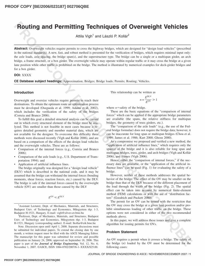
Hence, either the “comparison of internal forces,” if the nec-essary data are available, or the “application of the artificial in-fluence lines” can be used �Fig. 1� for evaluating the safety of abridge.

However, neither of these methods addresses the spatial be-havior of the bridge. The effect of the OV may be smaller on thebridge than that of the DLV because of the different placement ofthe load through the width of the bridge �Fig. 2�. The spatialeffect can be taken into account by numerical finite-elementmethod �FEM� calculations or with the aid of “distribution fac-tors” �Goodrich and Puckett 2000�.

The permit for an OV can be issued with the restriction thatthe OV may cross the bridge at a given lane position and/or pro-hibit simultaneous loading of other traffic on the bridge. Theseoptions were not considered in either of the two recommendedmethods above.

In this paper, we will address these issues and give a completealgorithm for issuing permits for OVs.

Problem Statement

An OV requires a permit when it crosses a bridge. The safety ofthe bridge �n� loaded by the OV must be determined for thefollowing cases:

1Assistant Lecturer, Dept. of Mechanics, Materials, and Structures,Budapest Univ. of Technology and Economics, Mûegyetem rkp. 1-3,Budapest H-1521, Hungary. E-mail: [email protected]

2Professor, Dept. of Mechanics, Materials, and Structures, BudapestUniv. of Technology and Economics, Mûegyetem rkp. 1-3, BudapestH-1521, Hungary �corresponding author�. E-mail: [email protected]

Note. Discussion open until April 1, 2008. Separate discussions mustbe submitted for individual papers. To extend the closing date by onemonth, a written request must be filed with the ASCE Managing Editor.The manuscript for this paper was submitted for review and possiblepublication on January 24, 2006; approved on September 18, 2006. Thispaper is part of the Journal of Bridge Engineering, Vol. 12, No. 6,November 1, 2007. ©ASCE, ISSN 1084-0702/2007/6-1–XXXX/$25.00.

JOURNAL OF BRIDGE ENGINEERING © ASCE / NOVEMBER/DECEMBER 2007 / 1

PROOF COPY [BE/2006/023187] 002706QBE

PROOF COPY [BE/2006/023187] 002706QBE

PROO

F COPY [BE/2006/023187] 002706Q

BE

• When the OV is part of the traffic �additional traffic loads areallowed on the bridge�;

• When the other traffic loads are not permitted �Fig. 3�; and• When the other traffic loads are not permitted and the OV

must go along the middle of the bridge �Fig. 2�c��.The OV may cross the bridge when n�1. Note that in the calcu-lation of n both the possible failure of the main load carrying

members and the failure of the deck, cross girders, etc., must beconsidered; the first will be referred to as “global” failure whilethe second will be referred to as “local” failure.

Approach

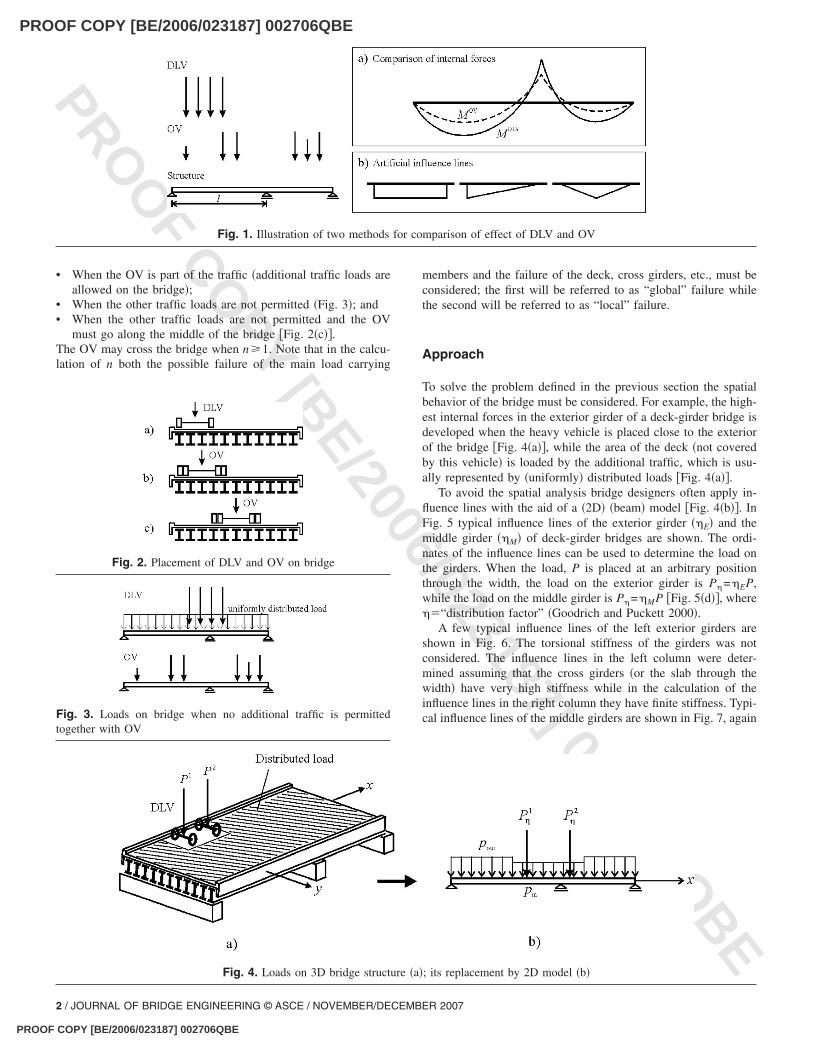
To solve the problem defined in the previous section the spatialbehavior of the bridge must be considered. For example, the high-est internal forces in the exterior girder of a deck-girder bridge isdeveloped when the heavy vehicle is placed close to the exteriorof the bridge �Fig. 4�a��, while the area of the deck �not coveredby this vehicle� is loaded by the additional traffic, which is usu-ally represented by �uniformly� distributed loads �Fig. 4�a��.

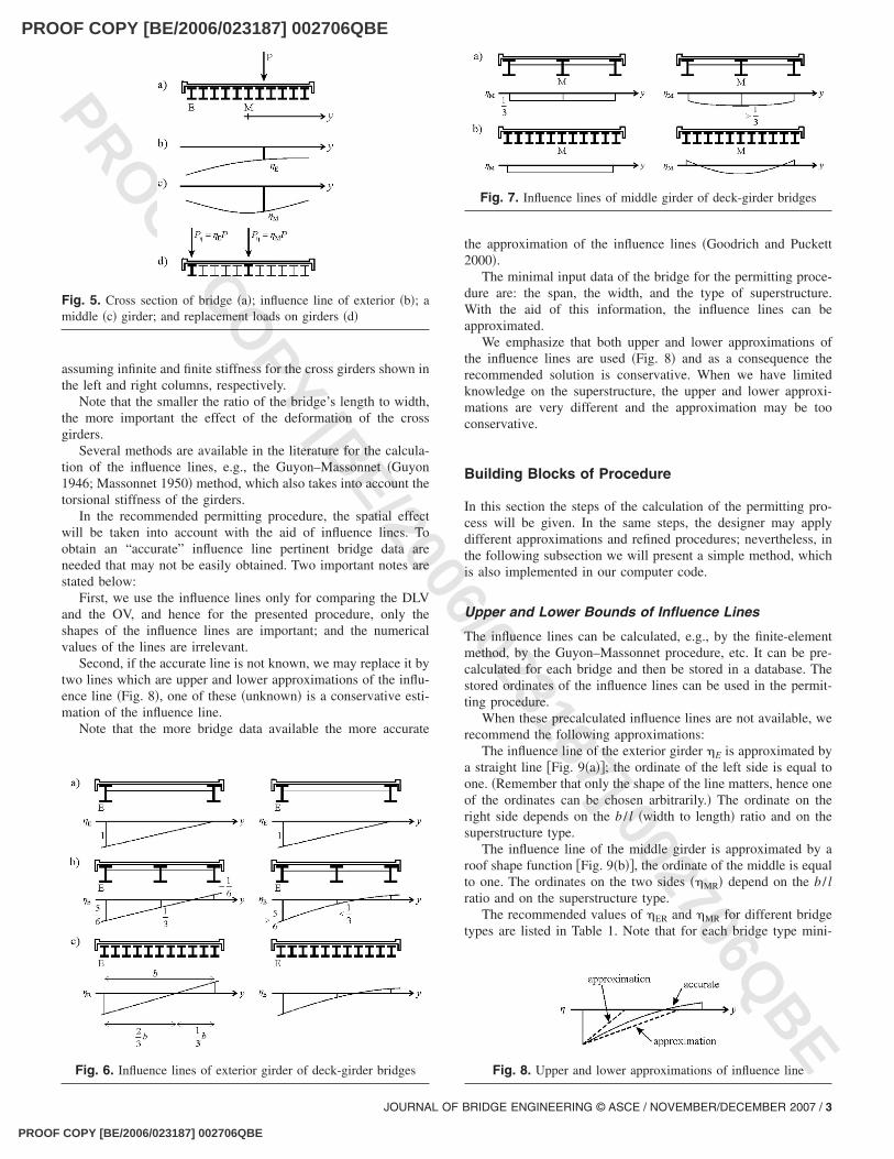
To avoid the spatial analysis bridge designers often apply in-fluence lines with the aid of a �2D� �beam� model �Fig. 4�b��. InFig. 5 typical influence lines of the exterior girder ��E� and themiddle girder ��M� of deck-girder bridges are shown. The ordi-nates of the influence lines can be used to determine the load onthe girders. When the load, P is placed at an arbitrary positionthrough the width, the load on the exterior girder is P�=�EP,while the load on the middle girder is P�=�MP �Fig. 5�d��, where��“distribution factor” �Goodrich and Puckett 2000�.

A few typical influence lines of the left exterior girders areshown in Fig. 6. The torsional stiffness of the girders was notconsidered. The influence lines in the left column were deter-mined assuming that the cross girders �or the slab through thewidth� have very high stiffness while in the calculation of theinfluence lines in the right column they have finite stiffness. Typi-cal influence lines of the middle girders are shown in Fig. 7, again

Fig. 1. Illustration of two methods for comparison of effect of DLV and OV

Fig. 2. Placement of DLV and OV on bridge

Fig. 3. Loads on bridge when no additional traffic is permittedtogether with OV

Fig. 4. Loads on 3D bridge structure �a�; its replacement by 2D model �b�

2 / JOURNAL OF BRIDGE ENGINEERING © ASCE / NOVEMBER/DECEMBER 2007

PROOF COPY [BE/2006/023187] 002706QBE

PROOF COPY [BE/2006/023187] 002706QBE

PROO

F COPY [BE/2006/023187] 002706Q

BE

assuming infinite and finite stiffness for the cross girders shown inthe left and right columns, respectively.

Note that the smaller the ratio of the bridge’s length to width,the more important the effect of the deformation of the crossgirders.

Several methods are available in the literature for the calcula-tion of the influence lines, e.g., the Guyon–Massonnet �Guyon1946; Massonnet 1950� method, which also takes into account thetorsional stiffness of the girders.

In the recommended permitting procedure, the spatial effectwill be taken into account with the aid of influence lines. Toobtain an “accurate” influence line pertinent bridge data areneeded that may not be easily obtained. Two important notes arestated below:

First, we use the influence lines only for comparing the DLVand the OV, and hence for the presented procedure, only theshapes of the influence lines are important; and the numericalvalues of the lines are irrelevant.

Second, if the accurate line is not known, we may replace it bytwo lines which are upper and lower approximations of the influ-ence line �Fig. 8�, one of these �unknown� is a conservative esti-mation of the influence line.

Note that the more bridge data available the more accurate

the approximation of the influence lines �Goodrich and Puckett2000�.

The minimal input data of the bridge for the permitting proce-dure are: the span, the width, and the type of superstructure.With the aid of this information, the influence lines can beapproximated.

We emphasize that both upper and lower approximations ofthe influence lines are used �Fig. 8� and as a consequence therecommended solution is conservative. When we have limitedknowledge on the superstructure, the upper and lower approxi-mations are very different and the approximation may be tooconservative.

Building Blocks of Procedure

In this section the steps of the calculation of the permitting pro-cess will be given. In the same steps, the designer may applydifferent approximations and refined procedures; nevertheless, inthe following subsection we will present a simple method, whichis also implemented in our computer code.

Upper and Lower Bounds of Influence Lines

The influence lines can be calculated, e.g., by the finite-elementmethod, by the Guyon–Massonnet procedure, etc. It can be pre-calculated for each bridge and then be stored in a database. Thestored ordinates of the influence lines can be used in the permit-ting procedure.

When these precalculated influence lines are not available, werecommend the following approximations:

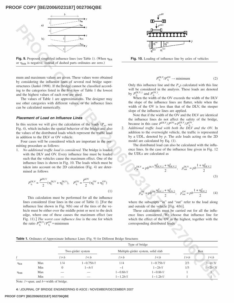
The influence line of the exterior girder �E is approximated bya straight line �Fig. 9�a��; the ordinate of the left side is equal toone. �Remember that only the shape of the line matters, hence oneof the ordinates can be chosen arbitrarily.� The ordinate on theright side depends on the b / l �width to length� ratio and on thesuperstructure type.

The influence line of the middle girder is approximated by aroof shape function �Fig. 9�b��, the ordinate of the middle is equalto one. The ordinates on the two sides ��MR� depend on the b / lratio and on the superstructure type.

The recommended values of �ER and �MR for different bridgetypes are listed in Table 1. Note that for each bridge type mini-

Fig. 5. Cross section of bridge �a�; influence line of exterior �b�; amiddle �c� girder; and replacement loads on girders �d�

Fig. 6. Influence lines of exterior girder of deck-girder bridges

Fig. 7. Influence lines of middle girder of deck-girder bridges

Fig. 8. Upper and lower approximations of influence line


PROOF COPY [BE/2006/023187] 002706QBE

PROOF COPY [BE/2006/023187] 002706QBE

PROO

F COPY [BE/2006/023187] 002706Q

BE

mum and maximum values are given. These values were obtainedby considering the influence lines of several real bridge super-structures �Jankó 1998�. If the bridge cannot be classified accord-ing to the categories listed in the first row of Table 1 the lowestand the highest values of each row are used.

The values of Table 1 are approximations. The designer mayuse other categories with different values, or the influence linescan be calculated numerically.

Placement of Load on Influence Lines

In this section we will give the calculation of the loads �P�, seeFig. 4�, which includes the spatial behavior of the bridge and alsothe values of the distributed loads which represent the traffic loadin addition to the DLV or OV vehicle.

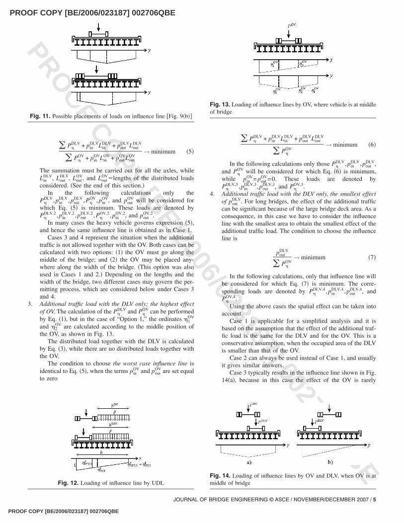
Four cases will be considered which are important in the per-mitting procedure as follows:1. No additional traffic load is considered. The bridge is loaded

with the DLV and OV. Every influence line must be loadedsuch that the vehicles cause the maximum effect. One of theinfluence lines is shown in Fig. 10. The loads which must betaken into account on the 2D calculation �Fig. 4� are deter-mined as follows

P�DLV =

PDLV

2��1

DLV + �2DLV�, P�

OV =POV

2��1

OV + �2OV�

�1�

This calculation must be performed for all the influencelines considered �four lines in the case of Table 1�. �For theinfluence line shown in Fig. 9�b� one of the tires of the ve-hicle must be either over the middle point or next to the deckedge, where one of these causes the maximum effect �seeFig. 11�.� The worst case influence line is the one for whichthe ratio P�

DLV/ P�OV�minimum

P�DLV/P�

OV → minimum �2�

Only this influence line and the P�s calculated with this linewill be considered in the analysis. These loads are denotedby P�

DLV,1 and P�OV,1.

When the width of the OV exceeds the width of the DLVthe slope of the influence lines are flatter, while when thewidth of the OV is less than that of the DLV, the steeperslope of the influence lines are applied.

Note that if the width of the OV and the DLV are identicalthe influence lines do not affect the safety of the bridge,because in this case PDLV/ POV= P�

DLV/ P�OV.

2. Additional traffic load with both the DLV and the OV. Inaddition to the overweight vehicle, the traffic is representedby a UDL, denoted by p. The axle loads acting on the 2Dmodel are calculated by Eq. �1�.

The distributed load can also be calculated with the influ-ence lines. In the case of the influence line given in Fig. 12the UDLs are calculated as

pinDLV = pbDLV�DLV,1

p + �DLV,2p

2, pout

DLV = pb1 + �DLV,2

p

2

�3�

pinOV = pbOV�OV,1

p + �OV,2p

2, pout

OV = pb1 + �OV,2

p

2�4�

where the subscripts “in” and “out” refer to the load alongand outside of the vehicle �Fig. 4�b��.

These calculations must be carried out for all the influ-ence lines considered. We choose that influence line forwhich the effect of the OV is the highest, together with thecorresponding distributed loads

Table 1. Ordinates of Approximate Influence Lines �Fig. 9� for Different Bridge Structures

Type of bridge

Two-girder system Multiple-girder system, solid slab Box

l l�b l�b l�b l�b l�b l�b

�ER Max 1/4 1−0.75b / l 1/4 1−0.75b / l 2/3 1−b /3l

Min 0 1−b / l −1 1−2b / l 1/3 1−2b /3l

�MR Max — — 1−0.8b / l 1−0.8b / l 1 1

Min — — 1−1.2b / l 1−1.2b / l 1 1

Note: l�span; and b�width of bridge.

Fig. 9. Proposed simplified influence lines �see Table 1�. �When �ER

or �MR is negative, instead of dashed parts ordinates are zero.�Fig. 10. Loading of influence line by axles of vehicles


PROOF COPY [BE/2006/023187] 002706QBE

PROOF COPY [BE/2006/023187] 002706QBE

PROO

F COPY [BE/2006/023187] 002706Q

BE

� P�DLV + pin

DLVLinDLV + pout

DLVLoutDLV

� P�OV + pin

OVLinOV + pout

OVLoutOV

→ minimum �5�

The summation must be carried out for all the axles, whileLin

DLV, LoutDLV, Lout

OV, and LoutOV�lengths of the distributed loads

considered. �See the end of this section.�In the following calculations only the

P�DLV, pin

DLV, poutDLV, P�

OV, pinOV, and pout

OV will be considered forwhich Eq. �5� is minimum. These loads are denoted byP�

DLV,2 , pinDLV,2 , pout

DLV,2 , P�OV,2 , pin

OV,2, and poutOV,2.

In many cases the heavy vehicle governs expression �5�,and hence the same influence line is obtained as in Case 1.

Cases 3 and 4 represent the situation when the additionaltraffic is not allowed together with the OV. Both cases can becalculated with two options: �1� the OV must go along themiddle of the bridge; and �2� the OV may be placed any-where along the width of the bridge. �This option was alsoused in Cases 1 and 2.� Depending on the lengths and thewidth of the bridge, two different cases may govern the per-mitting process, which are considered below under Cases 3and 4.

3. Additional traffic load with the DLV only; the highest effectof OV. The calculation of the P�

DLV and P�OV can be performed

by Eq. �1�, but in the case of “Option 1,” the ordinates �1OV

and �2OV are calculated according to the middle position of

the OV, as shown in Fig. 13.The distributed load together with the DLV is calculated

by Eq. �3�, while there are no distributed loads together withthe OV.

The condition to choose the worst case influence line isidentical to Eq. �5�, when the terms pin

OV and poutOV are set equal

to zero

� P�DLV + pin

DLVLinDLV + pout

DLVLoutDLV

� P�OV

→ minimum �6�

In the following calculations only those P�DLV, pin

DLV, poutDLV,

and P�OV will be considered for which Eq. �6� is minimum,

while pinOV= pout

OV=0. These loads are denoted byP�


DLV,3, and P�OV,3.

4. Additional traffic load with the DLV only, the smallest effectof pout

DLV. For long bridges, the effect of the additional trafficcan be significant because of the large bridge deck area. As aconsequence, in this case we have to consider the influenceline with the smallest area to obtain the smallest effect of theadditional traffic load. The condition to choose the influenceline is

poutDLV

� P�OV

→ minimum �7�

In the following calculations, only that influence line willbe considered for which Eq. �7� is minimum. The corre-sponding loads are denoted by P�


DLV,4, andP�

OV,4.Using the above cases the spatial effect can be taken into

account.Case 1 is applicable for a simplified analysis and it is

based on the assumption that the effect of the additional traf-fic load is the same for the DLV and for the OV. This is aconservative assumption, when the occupied area of the DLVis smaller than that of the OV.

Case 2 can always be used instead of Case 1, and usuallyit gives similar answers.

Case 3 typically results in the influence line shown in Fig.14�a�, because in this case the effect of the OV is rarely

Fig. 11. Possible placements of loads on influence line �Fig. 9�b��

Fig. 12. Loading of influence line by UDL

Fig. 13. Loading of influence lines by OV, where vehicle is at middleof bridge

Fig. 14. Loading of influence lines by OV and DLV, when OV is atmiddle of bridge


PROOF COPY [BE/2006/023187] 002706QBE

PROOF COPY [BE/2006/023187] 002706QBE

PROO

F COPY [BE/2006/023187] 002706Q

BE

affected by the placement of the OV at the middle. Case 4may likely result in the influence line shown in Fig. 14�b�,where the area is small.

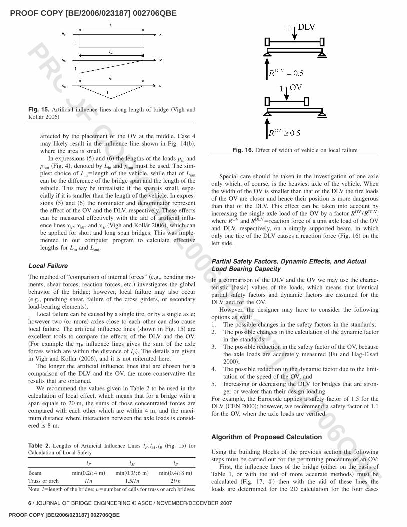
In expressions �5� and �6� the lengths of the loads pin andpout �Fig. 4�, denoted by Lin and pout must be used. The sim-plest choice of Lin�length of the vehicle, while that of Lout

can be the difference of the bridge span and the length of thevehicle. This may be unrealistic if the span is small, espe-cially if it is smaller than the length of the vehicle. In expres-sions �5� and �6� the nominator and denominator representthe effect of the OV and the DLV, respectively. These effectscan be measured effectively with the aid of artificial influ-ence lines �P, �M, and �B �Vigh and Kollár 2006�, which canbe applied for short and long span bridges. This was imple-mented in our computer program to calculate effectivelengths for Lin and Lout.

Local Failure

The method of “comparison of internal forces” �e.g., bending mo-ments, shear forces, reaction forces, etc.� investigates the globalbehavior of the bridge; however, local failure may also occur�e.g., punching shear, failure of the cross girders, or secondaryload-bearing elements�.

Local failure can be caused by a single tire, or by a single axle;however two �or more� axles close to each other can also causelocal failure. The artificial influence lines �shown in Fig. 15� areexcellent tools to compare the effects of the DLV and the OV.�For example the �P influence lines gives the sum of the axleforces which are within the distance of lP�. The details are givenin Vigh and Kollár �2006�, and it is not reiterated here.

The longer the artificial influence lines that are chosen for acomparison of the DLV and the OV, the more conservative theresults that are obtained.

We recommend the values given in Table 2 to be used in thecalculation of local effect, which means that for a bridge with aspan equals to 20 m, the sums of those concentrated forces arecompared with each other which are within 4 m, and the maxi-mum distance where interaction between the axle loads is consid-ered is 8 m.

Special care should be taken in the investigation of one axleonly which, of course, is the heaviest axle of the vehicle. Whenthe width of the OV is smaller than that of the DLV the tire loadsof the OV are closer and hence their position is more dangerousthan that of the DLV. This effect can be taken into account byincreasing the single axle load of the OV by a factor ROV/RDLV,where ROV and RDLV�reaction force of a unit axle load of the OVand DLV, respectively, on a simply supported beam, in whichonly one tire of the DLV causes a reaction force �Fig. 16� on theleft side.

Partial Safety Factors, Dynamic Effects, and ActualLoad Bearing Capacity

In a comparison of the DLV and the OV we may use the charac-teristic �basic� values of the loads, which means that identicalpartial safety factors and dynamic factors are assumed for theDLV and for the OV.

However, the designer may have to consider the followingoptions as well:1. The possible changes in the safety factors in the standards;2. The possible changes in the calculation of the dynamic factor

in the standards;3. The possible reduction in the safety factor of the OV, because

the axle loads are accurately measured �Fu and Hag-Elsafi2000�;

4. The possible reduction in the dynamic factor due to the limi-tation of the speed of the OV; and

5. Increasing or decreasing the DLV for bridges that are stron-ger or weaker than their design loading.

For example, the Eurocode applies a safety factor of 1.5 for theDLV �CEN 2000�; however, we recommend a safety factor of 1.1for the OV, when the axle loads are verified.

Algorithm of Proposed Calculation

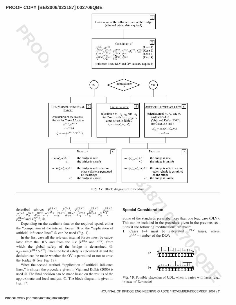
Using the building blocks of the previous section the followingsteps must be carried out for the permitting procedure of an OV:

First, the influence lines of the bridge �either on the basis ofTable 1, or with the aid of more accurate methods� must becalculated �Fig. 17, ①� then with the aid of these lines theloads are determined for the 2D calculation for the four cases

Table 2. Lengths of Artificial Influence Lines lP , lM , lB �Fig. 15� forCalculation of Local Safety

lP lM lB

Beam min�0.2l ;4 m� min�0.3l ;6 m� min�0.4l ;8 m�Truss or arch l /n 1.5l /n 2l /n

Note: l�length of the bridge; n�number of cells for truss or arch bridges.

Fig. 15. Artificial influence lines along length of bridge �Vigh andKollár 2006�

Fig. 16. Effect of width of vehicle on local failure


PROOF COPY [BE/2006/023187] 002706QBE

PROOF COPY [BE/2006/023187] 002706QBE

PROO

F COPY [BE/2006/023187] 002706Q

BE

described above: P�DLV,1, P�

OV,1, P�DLV,2, pin

DLV,2, poutDLV,2,

P�OV,2 , pin

OV,2 , poutOV,2 , P�


DLV,3 , P�OV,3 , P�

DLV,4 , pinDLV,4,

poutDLV,4and P�

OV,4, ②.Depending on the available data or the required speed, either

the “comparison of the internal forces” ③ or the “application ofartificial influence lines” ⑥ can be used �Fig. 1�.

In the first case all the relevant internal forces must be calcu-lated from the DLV and from the OV �EDLV and EOV�, fromwhich the global safety of the bridge is determined ③:ngl=min�EDLV/EOV�. Then the local safety is calculated ④ and thedecision can be made whether the OV is permitted or not to crossthe bridge ⑤ �see Fig. 17�.

When the second method, “application of artificial influencelines,” is chosen the procedure given in Vigh and Kollár �2006� isused ⑥. The final decision can be made based on the results of theapproximate and local analysis ⑦. The block diagram is given inFig. 17.

Special Consideration

Some of the standards prescribe more than one load case �DLV�.This can be included in the procedure given in the previous sec-tions if the following modifications are made:1. Cases 1–4 must be calculated nDLV times, where

nDLV�number of the DLV;

Fig. 17. Block diagram of procedure

Fig. 18. Possible placemen of UDL, when it varies with lanes �e.g.,in case of Eurocode�


PROOF COPY [BE/2006/023187] 002706QBE

PROOF COPY [BE/2006/023187] 002706QBE

PROO

F COPY [BE/2006/023187] 002706Q

BE

2. In the “comparison of the internal forces” EDLV must be cal-culated as the envelope of the internal forces of the nDLV

design load vehicles; and3. In the “comparison of artificial influence lines” and the cal-

culation of the local safety, EPDLV, EM

DLV, and EBDLV must be

calculated as the envelope of Es of the nDLV design loadvehicles.

Some of the standards �e.g., the Ontario Highway Bridge De-sign Code �Bakht and Jaeger 1984� and the Eurocode�, prescribedifferent UDLs in the different lanes of the bridge, while theassumed number of lanes depends on the width of the bridge �Fig.18�a��. In this case only the load calculation on the 2D model�step ② in Fig. 17� must be modified, however more than one loadcase must be taken into account, as illustrated for three lanes inFigs. 18�a and b�.

Numerical Examples

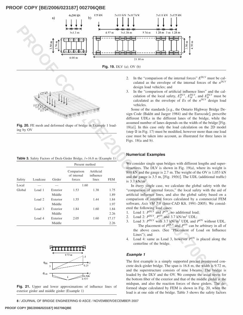
We consider single span bridges with different lengths and super-structures. The DLV is shown in Fig. 19�a�, where its weight is800 kN and the gauge is 2.7 m. The weight of the OV is 1,053 kNand the gauge is 3.5 m, �Fig. 19�b��. The UDL �additional traffic�is 3.7 kN/m2.

In every single case, we calculate the global safety with the“comparison of internal forces,” the local safety with the aid ofartificial influence lines, and also the global safety based on acomparison of internal forces calculated by a commercial FEMsoftware, Axis VM 7.0 �Inter-CAD Kft. 1991–2005�. We consid-ered the following load cases:1. Load 1: PDLV and POV, no additional load;2. Load 2: PDLV, POV and 3.7 kN/m2 UDL;3. Load 3: PDLV with 3.7 kN/m2 UDL and POV without UDL.

The placement of PDLV and POV can be arbitrary in all ofthe above cases. �See “Placement of Load on InfluenceLines”�; and

4. Load 4: same as Load 3, however POV is placed along thecenterline of the bridge.

Example 1

The first example is a simply supported precast prestressed con-crete deck-girder bridge. The span is 16.8 m, the width is 9.72 m,and the superstructure consists of nine I-beams. The bridge isloaded by the DLV and the OV. We compute the axial stress forthe bottom fiber of the exterior and that of the middle girder at themidspan, and also the reaction forces of these girders. The de-formed shape calculated by FEM is shown in Fig. 20, when theload is at one side of the bridge. Table 3 shows the safety factors

Table 3. Safety Factors of Deck-Girder Bridge, l=16.8 m �Example 1�

Present method

Safety Loadcase Girder

Comparisonof internal

forces

Artificialinfluence

lines FEM

Local — — 1.60

Global Load 1 Exterior 1.53 1.38 1.75

Middle 1.89

Load 2 Exterior 1.55 1.44 1.84

Middle 1.97


Middle 2.26

Load 4 Exterior 2.05 1.60 17.17

Middle 2.26

Fig. 19. DLV �a�; OV �b�

Fig. 20. FE mesh and deformed shape of bridge in Example 1 load-ing by OV

Fig. 21. Upper and lower approximations of influence lines ofexterior girder and middle girder �Example 1�


PROOF COPY [BE/2006/023187] 002706QBE

PROOF COPY [BE/2006/023187] 002706QBE

PROO

F COPY [BE/2006/023187] 002706Q

BE

of the methods for five load cases. The calculation shows that ourmethod is always on the safe side. The steps of our method are asfollows:1. The influence lines are determined first �Fig. 17�. From Table

1 �multiple-girder system, l�b� we obtain the lines shown inFig. 21.

2. Cases 1–4 are calculated �Fig. 17�, and the results are sum-marized in Table 4. Cases 1 and 2 are explained in detailbelow. The width of the OV exceeds the width of the DLV,hence the flattest influence line results in the lowestP�

DLV/ P�OV ratio �see Eq. �2��. The loads considered in the

analysis �Case 1� are: P�DLV=800 kN/2�0.969+0.761�

=692 kN and P�OV=1,053 kN/2�0.969+0.699�=878.3 kN

�see Fig. 22�a��.When the distributed loads are also taken into account

�Case 2�, Eq. �3� results in the influence line shown in Fig.22�b�. The DLV is represented by

P�DLV =

800 kN

2�1 + 0.705� = 697.14 kN

pinDLV = 3.7

kN

m2�4.46 m0.537 + 0.962

2

+ 1.76 m0.537 + 0.743

2� = 16.41

kN

m

poutDLV = 3.7

kN

m2 9.72 m0.537 + 1

2= 27.63

kN

m

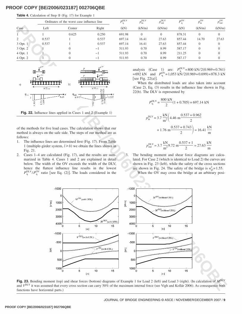
3. The bending moment and shear force diagrams are calcu-lated. For Case 2 �which is identical to Load 2� the curves areshown in Fig. 23 �left�, while the safety of the cross sectionsare shown in Fig. 24. The safety of the bridge is ngl

2 =1.55.When the OV may cross the bridge at an arbitrary posi-

Table 4. Calculation of Step ② �Fig. 17� for Example 1

Ordinates of the worst case influence line P�DLV pin

DLV poutDLV P�

OV pinOV pout

OV

Case Left Center Right �kN� �kN/m� �kN/m� �kN� �kN/m� �kN/m�

1 1 0.625 0.250 691.98 0 0 878.31 0 0

2 0.537 1 0.537 697.14 16.41 27.63 857.44 14.70 27.63

3 Opt. 1 0.537 1 0.537 697.14 16.41 27.63 857.44 0 0

3 Opt. 2 1 0 −1 511.93 0.70 8.99 587.17 0 0

4 Opt. 1 1 0 −1 511.93 0.70 8.99 211.25 0 0

4 Opt. 2 1 0 −1 511.93 0.70 8.99 587.17 0 0

Fig. 22. Influence lines applied in Cases 1 and 2 �Example 1�

Fig. 23. Bending moment �top� and shear forces �bottom� diagrams of Example 1 for Load 2 �left� and Load 3 �right�. �In calculation of MDLV

and VDLV it was assumed that every cross section can carry 50% of the maximum internal force �see Vigh and Kollár 2006�. As consequence bothfunctions have horizontal parts.�


PROOF COPY [BE/2006/023187] 002706QBE

PROOF COPY [BE/2006/023187] 002706QBE

PROO

F COPY [BE/2006/023187] 002706Q

BE

tion and the other traffic is prohibited �Load 3� either Case 3or Case 4 results in the lowest safety. In this example Case 3gives �Fig. 23 right� ngl

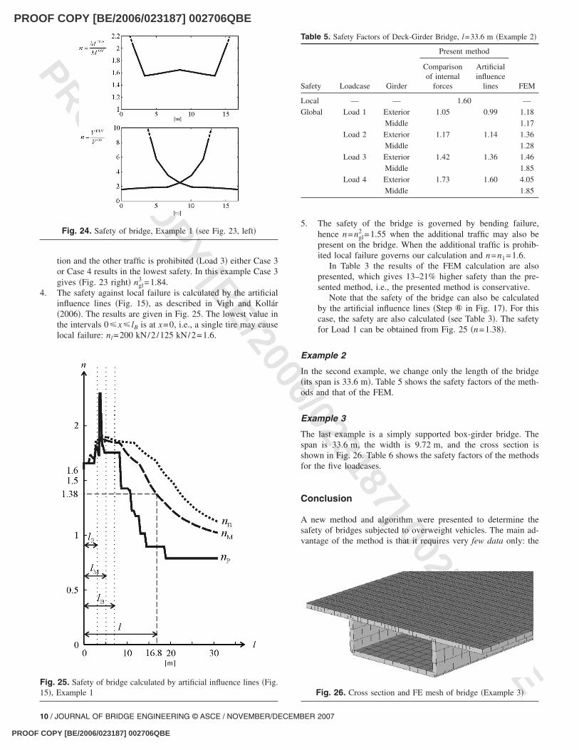
3 =1.84.4. The safety against local failure is calculated by the artificial

influence lines �Fig. 15�, as described in Vigh and Kollár�2006�. The results are given in Fig. 25. The lowest value inthe intervals 0�x� lB is at x=0, i.e., a single tire may causelocal failure: nl=200 kN/2/125 kN/2=1.6.

5. The safety of the bridge is governed by bending failure,hence n=ngl

2 =1.55 when the additional traffic may also bepresent on the bridge. When the additional traffic is prohib-ited local failure governs our calculation and n=n1=1.6.

In Table 3 the results of the FEM calculation are alsopresented, which gives 13–21% higher safety than the pre-sented method, i.e., the presented method is conservative.

Note that the safety of the bridge can also be calculatedby the artificial influence lines �Step ⑥ in Fig. 17�. For thiscase, the safety are also calculated �see Table 3�. The safetyfor Load 1 can be obtained from Fig. 25 �n=1.38�.

Example 2

In the second example, we change only the length of the bridge�its span is 33.6 m�. Table 5 shows the safety factors of the meth-ods and that of the FEM.

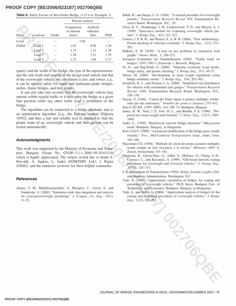
Example 3

The last example is a simply supported box-girder bridge. Thespan is 33.6 m, the width is 9.72 m, and the cross section isshown in Fig. 26. Table 6 shows the safety factors of the methodsfor the five loadcases.

Conclusion

A new method and algorithm were presented to determine thesafety of bridges subjected to overweight vehicles. The main ad-vantage of the method is that it requires very few data only: the

Table 5. Safety Factors of Deck-Girder Bridge, l=33.6 m �Example 2�

Present method



forces

Artificialinfluence

lines FEM

Local — — 1.60 —

Global Load 1 Exterior 1.05 0.99 1.18

Middle 1.17


Middle 1.28


Middle 1.85


Middle 1.85

Fig. 24. Safety of bridge, Example 1 �see Fig. 23, left�

Fig. 25. Safety of bridge calculated by artificial influence lines �Fig.15�, Example 1 Fig. 26. Cross section and FE mesh of bridge �Example 3�


PROOF COPY [BE/2006/023187] 002706QBE

PROOF COPY [BE/2006/023187] 002706QBE

PROO

F COPY [BE/2006/023187] 002706Q

BE

span�s� and the width of the bridge; the type of the superstructure;and the axle loads and spacing of the design load vehicle and thatof the overweight vehicle; the calculation is fast, and robust; e.g.,it can be applied safely for single and multispan girder bridges,arches, frame bridges, and box girders.

It can also take into account that the overweight vehicle mayoperate within regular traffic or it may cross the bridge at a givenlane position while any other traffic load is prohibited on thebridge.

The algorithm can be connected to a bridge databank, and toan optimization algorithm �e.g., the Dijkstra method �Dijkstra1959��, and thus a fast and reliable tool is obtained to find theproper route of an overweight vehicle and thus permits can beissued automatically.

Acknowledgments

This work was supported by the Ministry of Economy and Trans-port, Hungary �Grant No. GVOP–3.1.1–2004–05–0141/3.0�which is highly appreciated. The writers would like to thank A.Horváth, Á. Sapkás, L. Jankó �FÕMTERV Ltd.�, I. Rigler�UKIG�, and the unknown reviewer for their helpful comments.

References

Adams, T. M., Malaikrisanachalee, S., Blazquez, C., Lueck, S., andVonderohe, A. �2002�. “Enterprise-wide data integration and analysisfor oversize/overweight permitting.” J. Comput. Civ. Eng., 16�1�,11–22.

Bakht, B., and Jaeger, L. G. �1984�. “A rational procedure for overweightpermits.” Transportation Research Record. 950, Transportation Re-search Board, Washington, D.C., 59.

Chou, K. C., Deatherage, J. H., Leatherwood, T. D., and Khayat, A. J.�1999�. “Innovative method for evaluating overweight vehicle per-mits.” J. Bridge Eng., 4�3�, 221–227.

Correia, J. P. R. R., and Branco, F. A. B. B. �2006�. “New methodology:Permit checking of vehicular overloads.” J. Bridge Eng., 11�3�, 274–281.

Dijkstra, E. W. �1959�. “A note on two problems in connection withgraphs.” Numer. Math., 1, 269–271.

European Committee for Standardization �CEN�. “Traffic loads onbridges.” ENV 1991-3, Eurocode 1, Brussels, Belgium.

Fu, G., and Hag-Elsafi, O. �2000�. “Vehicular overloads: Load model,bridge safety, and permit checking.” J. Bridge Eng., 5�1�, 49–57.

Ghosn, M. �2000�. “Development of truck weight regulations usingbridge reliability model.” J. Bridge Eng., 5�4�, 293–303.

Goodrich, B. L., and Puckett, J. A. �2000�. “Simplified load distributionfor vehicles with nonstandard axle gauges.” Transportation ResearchRecord. 1696, Transportation Research Board, Washington, D.C.,158–170.

Guyon, Y. �1946�. “Calcul des Ponts larges á pouters multiples solidar-isées par des entretoises.” Annallés des ponts et chausses, 533–612.

Inter-CAD Kft. �1991–2005�. Axis VM 7.0, Budapest, Hungary.James, R. W., Noel, J. S., Furr, H. L., and Bonilla, F. E. �1986�. “Pro-

posed new truck weight limit formula.” J. Struct. Eng., 112�7�, 1589–1604.

Jankó, L., �1998�. “Reinforced concrete bridge structures.” Mûegyetemikiadó, Budapest, Hungary, in Hungarian.

Kurt, Carl E. �2000�. “A proposed modification of the bridge gross weightformula.” Proc., Mid-Continent Transportation Symp., Ames, Iowa,104–108.

Massonnet, Ch. �1950�. “Methode de calcul des ponts á pouters multiplestenant compte de leur résistance á la torsion.” Mémoires AIPC X,Zurich, Switzerland, 147–182.

Osegueda, R., Garcia-Diaz, A., Ashur, S., Melchor, O., Chang, S.-H.,Carrasco, C., and Kuyumcu, A. �1999�. “GIS-based network routingprocedures for overweight and oversized vehicles.” J. Transp. Eng.,125�4�, 324–331.

U.S. Department of Transportation �1994�. Bridge formula weights, Fed-eral Highway Administration, Washington, D.C.

Vigh, A. �2006�. “Approximate calculation of bridges for routing andpermitting of overweight vehicles.” Ph.D. thesis, Budapest Univ. ofTechnology and Economics, Budapest, Hungary, in Hungarian.

Vigh, A., and Kollár, L. �2006�. “Approximate analysis of bridges for therouting and permitting procedures of overweight vehicles.” J. BridgeEng., 11�3�, 282–292.

Table 6. Safety Factors of Box-Girder Bridge, l=33.6 m �Example 3�

Present method



forces

Artificialinfluence

lines FEM

Local — — 1.60 —

Global Load 1 — 1.01 0.96 1.20

Load 2 — 1.15 1.12 1.30

Load 3 — 1.58 1.51 1.79

Load 4 — 1.72 1.60 2.17


PROOF COPY [BE/2006/023187] 002706QBE

routing and permitting techniques of overweight vehicles · routing and permitting techniques of...

Documents